


1. Introduction
Non-Newtonian fluids exhibit interesting nonlinear material properties, which offer a range of very exciting practical benefits. Viscoelastic fluids, a subclass of non-Newtonian fluids, are no exception to this. This type of fluid involves mixing polymer additives with a solvent, which gives rise to interesting time-dependent flow dynamics not experienced in purely Newtonian flows (Steinberg Reference Steinberg2021). It is well known that the addition of these polymer molecules generates an anisotropic elastic stress contribution that transitions the flow to a chaotic regime, coined elastic turbulence (Groisman & Steinberg Reference Groisman and Steinberg2000, Reference Groisman and Steinberg2004). Unlike traditional turbulence, the nonlinearity of this chaotic regime is sourced from purely elastic instabilities, allowing for enhanced mixing capabilities at vanishingly low Reynolds numbers,  ${Re} \lesssim 1$. This level of nonlinearity of elastic instabilities is captured by the Weissenberg number
  $Wi$ which measures the relative elastic to viscous effects. Due to its inherent qualities, elastic turbulence has naturally emerged as an obvious solution to the long-encountered mixing challenges in microfluidics (Groisman & Steinberg Reference Groisman and Steinberg2001; Gan et al. Reference Gan, Lam, Nguyen, Tam and Yang2007).
The numerical simulation of elastic turbulence is far from a trivial task. The majority of previous numerical attempts have involved resolving the polymer field through constitutive polymer models, such as the Oldroyd-B model (Oldroyd Reference Oldroyd1950) and FENE-P model (Peterlin Reference Peterlin1961). Perhaps the greatest numerical difficulty encountered when solving either of these models arises due to the well-known high-Weissenberg-number problem (Alves, Oliveira & Pinho Reference Alves, Oliveira and Pinho2021). The excessive stretching of polymer molecules at high  $Wi$ numbers, a characteristic of elastic turbulence, leads to steep polymer stress gradients, which can quickly overwhelm numerical solvers if not treated correctly. These numerical issues can be partially alleviated through the use of high-resolution discretisation schemes (Kurganov & Tadmor Reference Kurganov and Tadmor2000; Vaithianathan et al. Reference Vaithianathan, Robert, Brasseur and Collins2006), enforcing strict polymer requirements (Vaithianathan & Collins Reference Vaithianathan and Collins2003) and the inclusion of a global artificial diffusivity term in the constitutive equations (Thomases Reference Thomases2011; Gupta & Vincenzi Reference Gupta and Vincenzi2019). However, because the elastic turbulence regime is driven purely by elastic instabilities, the global artificial diffusivity term has the potential to significantly influence the numerical solutions, which can lead to an incorrect physical interpretation of the chaotic regime, as demonstrated recently by Gupta & Vincenzi (Reference Gupta and Vincenzi2019). Although not imposing any artificial diffusivity would lead to an exact representation of elastic turbulence, the steep polymer stress gradients that develop would require significant grid resolutions and, hence, computational costs to overcome the numerical stability issues that ensue. In certain cases these stability issues can be partially alleviated through the local use of artificial diffusivity in only regions of high polymer stress gradients (Dubief et al. Reference Dubief, Terrapon, White, Shaqfeh, Moin and Lele2005). However, this localised approach has only been applied to drag-reducing viscoelastic flows with
  $Re\gg 1$ (Dubief et al. Reference Dubief, Terrapon, White, Shaqfeh, Moin and Lele2005). In the case of limited inertial effects (i.e. elastic turbulence,
  $Re\ll 1$), Gupta & Vincenzi (Reference Gupta and Vincenzi2019) argued that global artificial diffusivity has a much more significant effect on the flow than when inertial effects are more prominent, such as for elasto-inertial flows where high levels of artificial diffusivity do not alter the flow behaviour significantly. Furthermore, the additional complexities surrounding the careful treatment of solid boundaries and multicomponent flow interactions render most previous numerical studies to simplified flow configurations (Alves et al. Reference Alves, Oliveira and Pinho2021). These idealised benchmark cases attempt to recreate popular experimental periodic flow cases of elastic turbulence (Arora, Sureshkumar & Khomami Reference Arora, Sureshkumar and Khomami2002; Liu, Shelley & Zhang Reference Liu, Shelley and Zhang2012), and are often constrained to only two dimensions with fully periodic boundary conditions (PBCs). Nevertheless, these simplified cases have proved successful in qualitatively and quantitatively reproducing the main experimental observations of elastic turbulence, which includes unsteady velocity fluctuations (Gupta & Vincenzi Reference Gupta and Vincenzi2019), increased flow resistance (Berti et al. Reference Berti, Bistagnino, Boffetta, Celani and Musacchio2008), a broad range of temporal and spectral frequencies (Berti et al. Reference Berti, Bistagnino, Boffetta, Celani and Musacchio2008; Gupta & Vincenzi Reference Gupta and Vincenzi2019) and enhanced mixing (Plan et al. Reference Plan, Gupta, Vincenzi and Gibbon2017).
Three popular benchmarks with PBCs have emerged as appropriate tests to numerically simulate elastic turbulence, namely (i) the Kolmogorov forcing scheme (Berti et al. Reference Berti, Bistagnino, Boffetta, Celani and Musacchio2008; Plan et al. Reference Plan, Gupta, Vincenzi and Gibbon2017), (ii) the cellular forcing scheme (Plan et al. Reference Plan, Gupta, Vincenzi and Gibbon2017; Gupta & Vincenzi Reference Gupta and Vincenzi2019) and (iii) the four-roll mill case (Thomases & Shelley Reference Thomases and Shelley2009; Thomases Reference Thomases2011; Thomases, Shelley & Thiffeault Reference Thomases, Shelley and Thiffeault2011). All three benchmark cases involve imposing a constant external background force that drives the evolution of the flow through rotating and counter-rotating cylinders. From the three cases, the four-roll mill has arguably emerged as the most widely applied benchmark case for simulating elastic turbulence and will be considered in the current investigation. The reason for selecting the four-roll mill force is twofold. First, the regime generates a flow structure in which the straining and vortical regions are clearly separated, similar to the cellular forcing scheme considered by Gupta & Vincenzi (Reference Gupta and Vincenzi2019), this feature will turn out useful in highlighting the effect of periodicity on elastic turbulence. Second, the case is one of the limited but most widely used benchmark cases for the numerical simulation of viscoelastic fluids, allowing to investigate the main features of elastic turbulence with simplified PBCs. In their study, Thomases & Shelley (Reference Thomases and Shelley2009) conducted a numerical investigation into the transition and onset of elastic turbulence using the four-roll mill case. It was found that at small  $Wi$ numbers (i.e.
  $Wi\leq 5$) the flow was largely slaved to the initial symmetry and extensional geometry imposed by the background force. Interestingly, at moderate
  $Wi$ numbers (i.e.
  $5< Wi<9$), the flow experienced asymmetry, transitioning to a structurally dissimilar state dominated by a single large vortex. Beyond this, at even higher
  $Wi$ numbers (i.e.
  $Wi\geq 10$), the flow transitioned into a new state dominated by high velocity fluctuations. This new state showed persistent oscillatory behaviour with the production and destruction of smaller-scale vortices that promoted mixing. In a separate study, Thomases et al. (Reference Thomases, Shelley and Thiffeault2011) found that within this high-oscillatory regime, the flow dynamics transitioned from quasi-periodic (
 $Wi=10$) to fully periodic (
 $Wi=12,15$) and then to non-periodic (
 $Wi=20,30$). The numerical results were in partial agreement with popular experimental investigations of elastic turbulence in cross-channel flows (Arratia et al. Reference Arratia, Thomas, Diorio and Gollub2006), which also observed two flow instabilities: one in which the velocity field becomes strongly asymmetric, and a second in which it fluctuates non-periodically in time. However, an experimental study of the four-roll mill by Liu et al. (Reference Liu, Shelley and Zhang2012), which involved using sixteen rollers observed contrasting results. In their study, it was found that the transition into the oscillatory state was not a product of flow asymmetry. In fact, the experimental investigation outlined the differences in lattice geometry (i.e. number of rollers) as a potential explanation as to the absence of flow asymmetry. Similarly, in a numerical study by Gupta & Vincenzi (Reference Gupta and Vincenzi2019) exploring the effect of artificial diffusivity on elastic turbulence using the cellular forcing scheme, it was found that at high
  $Wi$ numbers the flow was largely slaved to the background driving force with distinct areas of vortical and strain-dominated regions. The investigation confirmed that any flow asymmetry experienced by the cellular forcing scheme was, in fact, a by-product of the excessive artificial stress diffusivity implemented to increase numerical stability. The study by Gupta & Vincenzi (Reference Gupta and Vincenzi2019) confirmed that the ability to accurately simulate the elastic turbulence regime is very sensitive to controlled parameters, and although the effect of artificial diffusivity has been explored in previous works (Thomases Reference Thomases2011; Gupta & Vincenzi Reference Gupta and Vincenzi2019), the role of PBCs in the elastic turbulence regime has been left largely unexplored.
The role of PBCs is to replicate the same characteristic flow (i.e. the unit cell) over all regions of the spatial domain in an infinite system. Given that the fundamental assumption of all fully periodic problems is an infinite system, the ability to replicate this inherently unphysical assumption numerically increases in accuracy with a larger number of unit cells, i.e. by increasing the periodicity. In fact, periodic problems require solving the same flow at least twice, which provides a great test of whether or not the numerical simulations can preserve the initial flow symmetry (Lecoanet et al. Reference Lecoanet, McCourt, Quataert, Burns, Vasil, Oishi, Brown, Stone and O'Leary2016). Furthermore, in active matter, such as microswimmers (De Graaf & Stenhammar Reference De Graaf and Stenhammar2017), it is well established that a large number of units cells is required to adequately represent PBCs due to a slow decay of the stresslet flow field. We shall see that, when applied to the four-roll mill case for viscoelastic fluids in the inertialess limit, the level of periodicity of the background force  $n$, which dictates the number of four-roll unit cells, greatly influences the late-time dynamics within the elastic turbulence regime. More specifically, it will be shown that the use of four rollers (i.e.
  $n=1$) will be inadequate to maintain the background symmetry of the initial forcing, leading to noticeable qualitative and quantitative differences with the results obtained using a larger number of rollers. We show that increasing the periodicity to
  $n=2, 3, 4$ and even
  $8$ (corresponding to
  $256$ rollers) leads to flow regimes that are still mostly confined to the effects of the background forcing, but transition into purely chaotic dynamics at later times, reminiscent of the experimental results obtained by Liu et al. (Reference Liu, Shelley and Zhang2012). Moreover, the results at the higher levels of periodicity fail to show any transition from quasi-periodicity and full periodicity, in contrast to results observed in the current study (
 $n=1$) and previous studies when using the four-roll mill (Thomases & Shelley Reference Thomases and Shelley2009; Thomases et al. Reference Thomases, Shelley and Thiffeault2011). In fact, all of the high-periodicity simulations transition to a purely chaotic state, with any quantitative differences being attributed to late-time chaos.
2. Numerical method
In the current investigation, we are interested in simulating the behaviour of incompressible viscoelastic fluids in the inertialess limit. Accordingly, two separate constitutive equations are required to characterise the hydrodynamic (i.e. solvent properties) and polymer (i.e. elastic properties) fields. The behaviour of the solvent can be described through the incompressible Navier–Stokes equations,
 \begin{gather} \boldsymbol{\nabla}\boldsymbol{\cdot}\boldsymbol{u}=0, \end{gather}
 \begin{gather}\frac{\partial\boldsymbol{u}}{\partial t}+\boldsymbol{u}\boldsymbol{\cdot}\boldsymbol{\nabla}\boldsymbol{u}={-}\boldsymbol{\nabla} p + \mu_s\boldsymbol{{\rm \Delta}}\boldsymbol{u}+\boldsymbol{F}+\boldsymbol{\nabla}\boldsymbol{\cdot}\boldsymbol{\sigma}_p, \end{gather}
where the symbols  $\rho$,
  $\mu _s$,
  $p$,
$p$,  $\boldsymbol {u}$ and
  $\boldsymbol {F}$ represent the density, the solvent dynamic viscosity, the pressure, the velocity and the external force contributions. Notably, the right-hand side includes an additional term,
  $\boldsymbol {\nabla }\boldsymbol {\cdot }\boldsymbol {\sigma }_p$, which accounts for the additional polymer stress contribution.
The constitutive equation for the polymer field involves representing polymer molecules as two beads (i.e. blocks of monomers) connected by a spring with a distance  $\boldsymbol {r}$. In this simplified system, the dumbbell springs undergo two processes, which include elongation due to a velocity gradient, as well as stress relaxation. To numerically model this description, a rank-2 conformation tensor
  ${\boldsymbol{\mathsf{C}}}$ describes the average orientation of the polymer chains at each point in the fluid,
  ${\boldsymbol{\mathsf{C}}}\equiv \langle r_ir_j \rangle$ (Vaithianathan & Collins Reference Vaithianathan and Collins2003). The simplest polymer model that incorporates these physical behaviours is the Oldroyd-B model (Oldroyd Reference Oldroyd1950),
 \begin{gather} \boldsymbol{\sigma}_p=\frac{\mu_p}{\tau_p} ({\boldsymbol{\mathsf{C}}}-{\boldsymbol{\mathsf{I}}}), \end{gather}
 \begin{gather}\frac{\partial{\boldsymbol{\mathsf{C}}}}{\partial t}+\boldsymbol{u}\boldsymbol{\cdot}\boldsymbol{\nabla} {\boldsymbol{\mathsf{C}}}={\boldsymbol{\mathsf{C}}}\boldsymbol{\cdot}(\boldsymbol{\nabla}\boldsymbol{u}) +(\boldsymbol{\nabla}\boldsymbol{u})^{\mathrm{T}}\boldsymbol{\cdot} {\boldsymbol{\mathsf{C}}}-\frac{1}{\tau_p}({\boldsymbol{\mathsf{C}}}-{\boldsymbol{\mathsf{I}}}) +\kappa\boldsymbol{{\rm \Delta}}{\boldsymbol{\mathsf{C}}}, \end{gather}
where the additional Laplace term in (2.2b),  $\kappa \boldsymbol {{\rm \Delta} }{\boldsymbol{\mathsf{C}}}$, is the artificial diffusivity.
  $\mu _p$ and
  ${\boldsymbol{\mathsf{I}}}$ are the polymer dynamic viscosity and identity tensor, respectively. A known limitation of the Oldroyd-B model is the unbounded molecular elongation of polymer molecules, which in certain flow conditions can lead to unphysical results, as the polymers stretch indefinitely. To ensure our results are not affected by the numerical limitations of the Oldroyd-B model, we conducted additional simulations in Appendix A using the FENE-P model (Peterlin Reference Peterlin1961), which imposes a maximum finite extensibility for the polymer molecules.
To resolve (2.1) and (2.2), a hybrid scheme from the authors previous study of viscoelastic instabilities (Dzanic, From & Sauret Reference Dzanic, From and Sauret2022) is used, comprising of a lattice Boltzmann (LB) model and a high-resolution finite difference scheme. More specifically, a single-relaxation time collision LB model with an explicit force coupling scheme is used to resolve (2.1) based on a mesoscopic description. The polymer contributions to the hydrodynamic field,  $\boldsymbol {\nabla }\boldsymbol {\cdot }\boldsymbol {\sigma }_p$, are incorporated directly in the LB collision using the popular ‘pressure method’ (Swift et al. Reference Swift, Orlandini, Osborn and Yeomans1996; Gupta, Sbragaglia & Scagliarini Reference Gupta, Sbragaglia and Scagliarini2015). The polymer solver involves directly resolving (2.2) using a fourth-order central difference scheme for the spatial gradients and a fourth-order Runge–Kutta scheme for the temporal evolution, ensuring that the accuracy of the discretisation schemes used lead to smooth and converged solutions. Given the definition,
  ${\boldsymbol{\mathsf{C}}}\equiv \langle r_i r_j \rangle$, it follows that the conformation tensor is a symmetric positive definite (SPD) matrix (Vaithianathan & Collins Reference Vaithianathan and Collins2003). However, the accumulation of errors resulting from steep polymer stress gradients at high
  $Wi$ can cause this property to be lost, leading to Hadamard instabilities (Sureshkumar & Beris Reference Sureshkumar and Beris1996). To overcome this, instead of solving for
  ${\boldsymbol{\mathsf{C}}}$, the Cholesky decomposition is applied to preserve the SPD property, i.e.
  ${\boldsymbol{\mathsf{C}}}={\boldsymbol{\mathsf{L}}}{\boldsymbol{\mathsf{L}}}^{\mathrm {T}}$, where
  ${\boldsymbol{\mathsf{L}}}$ is a lower-triangular matrix with elements
  $\mathsf{{L}}_{ij}$, such that
  $\mathsf{{L}}_{ij}=0$ for
  $j>i$ (Vaithianathan & Collins Reference Vaithianathan and Collins2003). The positivity of
  ${\boldsymbol{\mathsf{C}}}$ is confirmed by evolving the logarithmic transformation of the normal
  ${\boldsymbol{\mathsf{L}}}$ components (i.e.
  $\ln \mathsf{{L}}_{ii}$) (Vaithianathan & Collins Reference Vaithianathan and Collins2003). Equation (2.2) is a hyperbolic equation which lacks any diffusive terms to control the generation of sharp gradients (shocks) that occur at high
  $Wi$ numbers. Although the Cholesky-decomposition scheme eliminates the negative eigenvalues, an additional artificial diffusivity term
  $\kappa \boldsymbol {{\rm \Delta} }{\boldsymbol{\mathsf{C}}}$ (Vaithianathan & Collins Reference Vaithianathan and Collins2003; Gupta & Vincenzi Reference Gupta and Vincenzi2019) is added to the constitutive equations (e.g. (2.2)) to smooth out the steep gradients of
  ${\boldsymbol{\mathsf{C}}}$. The level of artificial diffusivity
  $\kappa$ is controlled by setting the Schmidt number
  $Sc=\nu _{s}/\kappa =10^{3}$ (i.e.
  $\kappa =10^{-4}$) in all of our simulations as done in previous studies of elastic turbulence (Thomases & Shelley Reference Thomases and Shelley2009; Thomases et al. Reference Thomases, Shelley and Thiffeault2011; Gupta & Vincenzi Reference Gupta and Vincenzi2019), where
  $\nu _{s}$ is the kinematic viscosity of the solvent. Although this level of diffusivity was found to affect the elastic turbulent regime for the cellular forcing scheme (Gupta & Vincenzi Reference Gupta and Vincenzi2019), we find that this value with true-periodic-boundary conditions preserves the background forcing symmetry and late-time chaos dynamics for the four-roll mill, as is shown in § 3. We also further control the effect of steep polymer stress gradients by treating the advection term,
  $\boldsymbol {u}{\,\boldsymbol {\cdot }\,}\boldsymbol {\nabla } {\boldsymbol{\mathsf{C}}}$, according to the high-resolution Kurganov–Tadmor (KT) scheme (Kurganov & Tadmor Reference Kurganov and Tadmor2000; Vaithianathan et al. Reference Vaithianathan, Robert, Brasseur and Collins2006).
Equations (2.1) and (2.2) are solved within a double periodic two-dimensional domain  $\boldsymbol {x} [0, n \times 2{\rm \pi} ]^{2}$ on a symmetric square grid with
  $(n \times N)^{2}$ grid points, subjected to
  $n$ levels of the constant four-roll mill force geometry (Thomases & Shelley Reference Thomases and Shelley2009),
 \begin{equation} \boldsymbol{F} (\boldsymbol{x}) = ( F_0\sin(K{x})\cos (K{y}), \quad -F_0\cos(K{x})\sin(K{y}) ), \end{equation}
where the spatial frequency  $K=1$ is kept constant to admit the four-roll mill geometry in each unit cell
  $[0, 2{\rm \pi} ]^{2}$ with
  $N$ number of grid points. As such, the grid resolution
  ${\rm \Delta} x = 2{\rm \pi} /N$ and the level of periodicity, defined through the parameter
  $n\geq 1$, sets the quantity of unit cells (i.e.
  $n = 1$ admits the standard four-roll mill benchmark case) (Thomases & Shelley Reference Thomases and Shelley2009; Thomases et al. Reference Thomases, Shelley and Thiffeault2011). This is possible because the four-roll mill force geometry (2.3) has a reverse-reflect symmetry property, as is required by PBCs. Here
  $F_0$ is the force amplitude fixed to
  $F_0 = 2U_0\nu _s K^{2}$, thus resulting in a turnover time,
  $T = 2\nu _s K/F_0$, where
  $U_0$ is the characteristic velocity formally defined further in the following.
To simulate elastic turbulence using the four-roll mill benchmark a small perturbation is added to the initial conformation tensor,  ${\boldsymbol{\mathsf{C}}}(\boldsymbol {x},0)={\boldsymbol{\mathsf{I}}}$. Here the same initial perturbation originally proposed in Thomases & Shelley (Reference Thomases and Shelley2009) is used and, as done for (2.3), repeated over
  $n$-levels of periodicity, i.e.
 \begin{equation} {\boldsymbol{\mathsf{C}}}(\boldsymbol{x},0) = {\boldsymbol{\mathsf{I}}} + \begin{pmatrix} \delta \cos(Ky) \psi(x) & -\delta\sin(Kx)\cos(2Ky) \\ -\delta\sin(Kx)\cos(2Ky) & \delta \cos(Kx) \psi(y) \end{pmatrix}, \end{equation}
with  $\delta = 0.01$ and
  $\psi (z)=2\sin (Kz)- 3/2\sin (2Kz),\ z:=x,y$. It is noted that, similar to the four-roll mill geometry (2.3), the initial perturbation (2.4) has the symmetry reverse-reflect property required by PBCs. In summary, any
  $n$ case (for
  $n\neq 0$) yield the same physical problem, meaning that cases
  $n\gneq 1$ essentially solve the same four-roll mill problem
  $n^{2}$ times [
 $O(n^{2})$ due to periodicity in both principle axis]. To assess the effect of periodicity on the flow, we perform simulations for
  $n = 1, 2, 3$ and
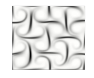
  $4$, corresponding to 4 (i.e. the standard case), 16, 36 and 64 rollers, respectively, as illustrated in figure 1. For typographical convenience, throughout this work these cases will be referred to as R4, R16, R36 and R64, respectively.

Figure 1. Initial normalised vorticity field of the four-roll mill forcing with (a)  $n=1$, (b)
  $n=2$, (c)
  $n=3$ and (d)
  $n=4$, which are referred by their corresponding
  $n^{2}$ number of rollers, namely, R4, R16, R36 and R64, respectively.
Following previous investigations of elastic turbulence (Berti et al. Reference Berti, Bistagnino, Boffetta, Celani and Musacchio2008; Plan et al. Reference Plan, Gupta, Vincenzi and Gibbon2017), we admit the flow to vanishingly low levels of inertia by setting  ${Re}$ below the critical value at which inertial instabilities arise,
  ${Re}_c=\sqrt {2}$ (Gotoh & Yamada Reference Gotoh and Yamada1984). The incompressibility of the hydrodynamic field is also ensured by setting the Mach number,
  $Ma\ll 0.3$. This allows us to easily retrieve the characteristic velocity,
  $U_0=c_s Ma$, which can be used to obtain
  $\nu _s=U_0/{Re}K$. (Note,
  $c_s=1/\sqrt {3}$ for the LB model used in this work. For more details, see Dzanic et al. (Reference Dzanic, From and Sauret2022).) To define the behaviour of the polymer field, we set the concentration using the parameter,
  $\beta =\nu _{p}/\nu _{s}$, which measures the relative polymer viscosity,
  $\nu _p$, to the solvent viscosity,
  $\nu _{s}$. The value
  $\beta =0.5$ will be fixed in our simulations to match previous numerical (Thomases & Shelley Reference Thomases and Shelley2009; Thomases et al. Reference Thomases, Shelley and Thiffeault2011) and experimental investigations (Arratia et al. Reference Arratia, Thomas, Diorio and Gollub2006). We control the level of polymer deformability by the Weissenberg number
  $Wi=\tau _p/T$ by setting the polymer relaxation,
  $\tau _p=WiT$, which is a direct measure of the polymer elasticity.
To summarise, the investigation will study the effect of the periodicity in the four-roll mill problem for elastic turbulence, whereby the level of periodicity is controlled by increasing  $n$. We note, that PBCs are inherently unphysical to begin with and are idealised assumptions used to simplify more complex systems, even for very high levels of periodicity. As such, the purpose of this investigation is not to imply that an accurate or exact level of periodicity exists when simulating elastic turbulence, but instead demonstrate the effect of different levels of periodicity, especially the numerical artefacts that ensue at lower levels of periodicity (i.e.
  $n=1$). Simulations will be conducted over
  $n=1, 2, 3$ and
  $4$ (denoted by R4, R16, R36 and R64, respectively) as shown in figure 1. All simulations will be conducted with
  $N^{2}=128^{2}$ grid points in a single unit cell (i.e. total
  $(n\times 128)^{2}$ grid points) using the Oldroyd-B model (analogous results for the FENE-P model are presented in Appendix A) at
  $Ma=0.01$,
  ${Re}={Re}_c/\sqrt {2} = 1$,
  $Sc=10^{3}$,
  $\beta =0.5$ and
  $Wi=10$. Dependence on
  $Wi$ is checked by running the same simulations for
  $5\leq Wi \leq 20$. Note, additional simulations with different parameters are reported in the supplementary material and movies are available at https://doi.org/10.1017/jfm.2022.103 and support the results presented in the following section.
3. Results
First, in figure 2(a) we show the time series of the first component of the conformation tensor  $\mathsf{{C}}_{xx}$ at the central stagnation point
  $[{\rm \pi},{\rm \pi} ]$ at the early stages of the flow, prior to the onset of viscoelastic instabilities (i.e.
  $0\leq t/T \leq 400$). As expected, all
  $n$ levels of periodicity retrieve the exact same evolutions for the polymer field. Initially, the polymers experience excessive stretching due to the high level of friction between the solvent and the polymer molecules, reaching a maximum extension within
  $t\approx 10T$. Beyond this maximum peak, the velocity gradients in (2.2), which drive the polymer stretching are no longer strong enough due to the transfer of kinetic energy to elastic energy, thus resulting in a noticeable steady state. Qualitatively, figures 2(b) and 2(c) show that during this stage, the flow is still slaved to the initial four-roll mill forcing symmetry. This steady-state region begins to break down as early as
  $t\approx 200T$, due to the presence of artificial diffusivity, causing the polymers to gradually relax back towards their initial equilibrium state (i.e.
  ${\boldsymbol{\mathsf{C}}}={\boldsymbol{\mathsf{I}}}$). This period of relaxation is reflected by a loss of the initial flow symmetry (as depicted in figures 3 and 4, and discussed shortly), as observed in previous studies of the four-roll mill (Thomases & Shelley Reference Thomases and Shelley2009; Thomases et al. Reference Thomases, Shelley and Thiffeault2011).

Figure 2. (a) Time series of the first component of the conformation tensor  $\mathsf{{C}}_{xx}$ at the position
  $[{\rm \pi},{\rm \pi} ]$ for the initial steady-state region corresponding to
 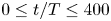 $0\leq t/T \leq 400$. Results are compared at different levels of periodicity, namely, the R4 (black solid), R16 (red solid), R36 (blue solid) and R64 (green dashed) case at
  $Wi=10$. A representative snapshot of (b) the vorticity and (c) the trace of conformation tensor,
  $\mathrm {tr}({\boldsymbol{\mathsf{C}}})$, at steady-state region corresponding to
  $t=100T$.

Figure 3. Contour plots for the vorticity field taken at the initial onset of asymmetry at  $t=300T$ (top row) and at the later stage corresponding to
  $t=1300T$ (bottom row) for each case, from left to right: R4, R16, R36 and R64 at
  $Wi=10$. Note, for the R16, R36 and R64 cases, the vorticity field is extracted for a single unit cell of size
  $[0\ 2{\rm \pi} ]$. The full domain contour plots can be found in the supplementary material and movies.

Figure 4. Contour plots for the conformation tensor trace  $\mathrm {tr}({\boldsymbol{\mathsf{C}}})$ at
  $Wi=10$ taken at the initial onset of asymmetry at
  $t=300T$ (top row) and at the later stage corresponding to
  $t=1300T$ (bottom row) for each case, from left to right: R4, R16, R36 and R64. Note, for the R16, R36 and R64 cases, the polymer trace field is extracted from the unit cell
  $[0, 2{\rm \pi} ]^{2}$. The full domain contour plots can be found in the supplementary material and movies.
The vorticity and the conformation tensor trace,  $\mathrm {tr}({\boldsymbol{\mathsf{C}}})$, contour fields are shown in figures 3 and 4, respectively, for all
  $n$ cases at the initial symmetry breakdown at
  $t=300T$ (top row) and within the chaotic elastic turbulent regime at
  $t=1300T$ (bottom row). Note, all results presented hereinafter for higher levels of periodicity (
 $n\gneq 1$) are sampled in a representative unit cell
  $[0,2{\rm \pi} ]^{2}$, and full domain results are included in the supplementary material and movies. The top row of figures 3 and 4 show that all levels of periodicity experience the same initial breakdown in symmetry originally observed by Thomases & Shelley (Reference Thomases and Shelley2009) and Thomases et al. (Reference Thomases, Shelley and Thiffeault2011) and can be attributed to the presence of artificial diffusivity (Gupta & Vincenzi Reference Gupta and Vincenzi2019), which unphysically stretches the polymers into the vortical regions of the flow, destabilising the initial forcing structure. However, at the later stages of the unsteady regime, the different periodicity levels contribute to contrasting qualitative differences observed in the vorticity and polymer fields. For instance, when observing the vorticity field for the classic four-roll mill case (
 $n=1$), corresponding to the left column in figure 3, once the flow transitions into the chaotic regime, the spatial structure of the flow departs from the initial symmetry imposed by the background force (refer to figures 2b and 2c). However, at the later stages, the R4 vorticity field is largely dominated by a single leading vortex, which cycles around all of the quadrants of the unit cell (Thomases & Shelley Reference Thomases and Shelley2009; Thomases et al. Reference Thomases, Shelley and Thiffeault2011). Only some of the remaining vortices continue to exist, whereas the remaining quadrants experience small patches of positive and negative vortices which contaminate the four-roll mill geometry of the base flow. In contrast, at higher periodicity
  $n\gneq 1$, figure 3 shows that the vorticity fields are slightly perturbed from the initial symmetry, however unlike the R4 case, the large-scale structures of the flow are still mostly adhering to the background force. The behaviour of the polymer field at the later stages also shows the same qualitative differences seen for the vorticity field in the regimes between the standard level (
 $n=1$) and all higher levels (
 $n\gneq 1$) of periodicity (figure 4 (bottom row)). In particular, in the case of higher periodicity
  $n\gneq 1$, the effect of the rollers on the polymer field is still noticeable. As a result, highly stretched polymers are found mostly in strain-dominated regions of the flow, situated in-between the rollers, whereas weakly stretched polymers are located in the vortical regions, where they are quickly contracted. However, for the R4 case, in figure 4 (bottom left), it is clear that the polymer molecules are no longer strictly stretched along the incoming and outgoing streamlines of the extensional stagnation points.
These results are similar to the results observed for the cellular forcing scheme at  $Sc=10^{3}$ by Gupta & Vincenzi (Reference Gupta and Vincenzi2019), who observed that the flow asymmetry was induced by artificial diffusivity, suppressing the true chaotic nature of the elastic turbulence regime. Here, we observe similar results for the four-roll mill, as all four periodic regimes experience an initial symmetry breakdown at
  $t\approx 300T$ due to the presence of artificial diffusivity (refer to figures 3 and 4 (top row)). However, the breakdown in symmetry is partly recovered by the higher periodicity cases (i.e.
  $n\gneq 1$), as the vorticity and polymer fields quickly retain the noticeable background forcing effects (refer to figures 3 and 4 (bottom row)). Notably, the background forcing symmetry for
  $n\gneq 1$ is not fully recovered, especially when compared with results without the use of global artificial diffusivity (Gupta & Vincenzi Reference Gupta and Vincenzi2019). This is reflected in figure 3, as some vortical cells are still slightly perturbed into unphysical regions of the flow, and is largely attributed to the remaining effects of artificial diffusivity. Nevertheless, the results at the later stages clearly show that the artefacts induced by artificial diffusivity reduce with increasing periodicity. On the other hand, the R4 case (
 $n=1$) is severely affected by the initial loss of symmetry induced by artificial diffusivity and is unable to recover the background forcing symmetry. The lack of periodicity in both directions causes the single leading vortex to remain throughout time and cycle around all four quadrants within a unit cell. In fact, an additional simulation was conducted increasing the periodicity in only one of the principal axis, specifically
  $x=[0,4{\rm \pi} ]$ and
  $y=[0,2{\rm \pi} ]$ corresponding to eight rollers (denoted R8, see Appendix B), which resulted in the same loss of symmetry as R4, supporting that this is an issue with the double-periodic requirements of the flow, as opposed to simply increasing the quantity of rollers.
Furthermore, we also show that the flow asymmetry is not induced numerically by a lack of spatial resolution (see the supplementary material and movies) and it is also not modified by the nonlinearity of the elastic force (see Appendix A). The differences in behaviour observed across all levels of periodicity are further confirmed in the analogous animations provided in the supplementary material and movies. Ultimately, we observe that our current results at higher levels of periodicity are reminiscent of the true solutions obtained by Gupta & Vincenzi (Reference Gupta and Vincenzi2019) for the cellular forcing scheme with zero artificial diffusivity (i.e. symmetric flow with fully chaotic behaviour in the elastic turbulent regime). Note, given the shared behaviour between figures 3 and 4, the remainder of the paper predominantly focuses on analysing the polymer field, with analogous results obtained for the hydrodynamic field.
In figure 5 we compare the fully evolved time series for  $\mathsf{{C}}_{xx}$ at the central stagnation point [
 ${\rm \pi}$,
  ${\rm \pi}$] at
  $Wi=10$ over the period
  $0\leq t/T \leq 2500$. For all of the different levels of periodicity, it can be seen that beyond the early and steady stages (for which all
  $n$ conform, see figure 2), the dynamics of the flow transition into a transient state at
  $t\approx 500T$. For the R4 case (
 $n=1$), in figure 5(a), this new transient regime first transitions into slow oscillations, which speed up over time. In fact, the high-oscillatory behaviour observed at the later time steps reflects quasi-periodic dynamics. These results are in full agreement with previous studies of the four-roll mill (Thomases & Shelley Reference Thomases and Shelley2009; Thomases et al. Reference Thomases, Shelley and Thiffeault2011), whereby qualitatively the quasi-periodic regime reflects a single dominant vortex which cycles between the four quadrants of a unit cell, as shown in figure 3(a). This quasi-periodic regime is also observed for the R8 case in Appendix B and, albeit different late-time dynamics are obtained compared to the standard R4 case, the dynamics observed strongly reflect the presence of a leading vortex. Nevertheless, this further supports that this is a numerical issue with the double-periodic requirements of the problem, as opposed to simply increasing the number of rollers. Interestingly, for higher levels of periodicity
  $n\gneq 1$, in figures 5(b)–5(d), the behaviour of the transient regime is completely different. It can be seen that the high-oscillatory regime is much more chaotic and transitions much more rapidly, showing no emerging periodic flow pattern. This purely chaotic regime is reminiscent of the countless experimental and numerical studies of elastic turbulence (Arratia et al. Reference Arratia, Thomas, Diorio and Gollub2006; Qin & Arratia Reference Qin and Arratia2017; Gupta & Vincenzi Reference Gupta and Vincenzi2019; Steinberg Reference Steinberg2021), which also observe highly transient flow fluctuations at excessive polymer stretching. The study by Thomases et al. (Reference Thomases, Shelley and Thiffeault2011) also observed similar behaviour for the four-roll mill case (
 $n=1$) with higher elastic effects, corresponding to
  $Wi=20$ and
  $30$. However, the high-frequency flow fluctuations of the
  $n\gneq 1$ cases observed here are fundamentally different; a key quality is that these fluctuations albeit perturbing the initial four-roll vortical structure still mostly adhere to the background forcing effects, as shown in figures 3 and 4, reminiscent of experimental observations by Liu et al. (Reference Liu, Shelley and Zhang2012) and the recent numerical study by Gupta & Vincenzi (Reference Gupta and Vincenzi2019). Note, the behaviour of the hydrodynamic field shows analogous results to the polymer field (refer to Appendix C).

Figure 5. Time series of the first component of the conformation tensor  $\mathsf{{C}}_{xx}$ at the position
  $[{\rm \pi},{\rm \pi} ]$ taken over
  $0\leq t/T \leq 2500$. Results are compared at different levels of periodicity, namely, (a) R4 (black), (b) R16 (red), (c) R36 (blue) and (d) R64 (green) at
  $Wi=10$.
To further characterise the behaviour of the different levels of periodicity within the elastic turbulence regime, we examine the temporal fast Fourier transform (FFT) of  $\mathsf{{C}}_{xx}$ (figure 6). We find again that the standard level of imposed periodicity of the R4 case has a strong effect on the flow (figure 6a). For this regime, as first discovered by Thomases et al. (Reference Thomases, Shelley and Thiffeault2011), the quasi-periodic dynamics observed in figure 5(a) is characterised by two dominant frequencies,
  $\omega _1$ and
  $\omega _2$, with all other large activated modes being sums, differences, and harmonics of these two frequencies. On the other hand, figures 6(b)–6(d) shows that for
  $n>1$, the polymer field experiences a broad range of temporal scales. The broad-band spectrum is characteristic of the chaotic elastic turbulent regime and has been observed in various previous experimental (Groisman & Steinberg Reference Groisman and Steinberg2000; Pan et al. Reference Pan, Morozov, Wagner and Arratia2013; Steinberg Reference Steinberg2021) and numerical studies (Berti et al. Reference Berti, Bistagnino, Boffetta, Celani and Musacchio2008; Grilli, Vazquez-Quesada & Ellero Reference Grilli, Vazquez-Quesada and Ellero2013; van Buel, Schaaf & Stark Reference van Buel, Schaaf and Stark2018). Moreover, the multi-frequency oscillating spectrum was also observed in the experimental study by Liu et al. (Reference Liu, Shelley and Zhang2012) of a 16-roll mill geometry for
  $Wi=8.42$, thus aligning closely with the chaotic behaviour of our higher periodicity results. Overall, it is clear that the use of only R4 (
 $n=1$) suppresses the true chaotic nature of the elastic turbulent regime, which is attributed to the lower levels of periodicity causing the characteristic dynamics of the system to periodically cycle around the domain.

Figure 6. The temporal fast Fourier transform (FFT) of  $Cxx$ at the position [
 ${\rm \pi},{\rm \pi}$] taken over the chaotic elastic turbulent regime for the (a) R4, (b) R16, (c) R36 and (d) R64 cases at
  $Wi=10$. The two dominant frequencies
  $\omega _1$ and
  $\omega _2$ are highlighted for the R4 case in (a).
We further examine this behaviour by investigating the change in dynamics for the polymer field at different  $Wi$ numbers for the R4 and R16 cases in figure 7. It can be seen that for both cases, the speed and frequency of oscillations increase with the
  $Wi$ number, which has also been observed in previous investigations of elastic turbulence (Arratia et al. Reference Arratia, Thomas, Diorio and Gollub2006; van Buel et al. Reference van Buel, Schaaf and Stark2018; Steinberg Reference Steinberg2021), however, the dynamics were observed across an entirely different range. Figure 7(a) shows that the R4 case at
  $Wi=5$ maintains a steady state over time and commences to transition into the transient regime at
  $Wi=6$, as reflected by the small-amplitude oscillations. At higher
  $Wi$ numbers the dynamics of the R4 (
 $n=1$) transition into various periodic states, as discovered originally by Thomases & Shelley (Reference Thomases and Shelley2009) and Thomases et al. (Reference Thomases, Shelley and Thiffeault2011). At
  $Wi=10$ the flow transitions into the quasi-periodic regime, as discussed earlier, before reaching a fully periodic state at
  $Wi=15$. Beyond this, at
  $Wi=20$ the polymer field is more chaotic and undergoes aperiodic dynamics. In figure 7(b) we see that for the R16 case the transition from quasi-periodic to fully periodic dynamics is not observed even for a wider range of
  $Wi$ numbers. The experimental investigation on the four-roll mill by Liu et al. (Reference Liu, Shelley and Zhang2012), which involved using 16 rollers (i.e. equivalent to
  $n=2$ (R16)), outlined the potential to obtain richer dynamics based on the lattice geometry. Here, we see that similar to the R4 case, the regime with higher levels of periodicity (R16 in figure 7b) also undergoes a transition into the oscillatory regime at
  $Wi=6$. However, the R16 case immediately transitions into the aperiodic (i.e. chaotic) regime (
 $Wi\approx 6.5$; note,
  $Wi$ numbers increased at increments of
  $0.5$), whereas the R4 case continues to experience slow oscillations which are followed by a transition into the quasi-periodic regime for
  $Wi\geq 9$. When comparing the two aperiodic regimes at
  $Wi=20$, it can be seen that the R16 case is more chaotic, experiencing higher frequency fluctuations in the polymer field, as well as a faster transition into the chaotic regime. Qualitatively, the R16 regime at
  $Wi=20$ is no longer slaved to the background forcing and experiences richer dynamics which resemble the R16 experimental results by Liu et al. (Reference Liu, Shelley and Zhang2012). Overall, these results show that the differences in dynamics between the R4 case and the solutions with higher levels of periodicity (
 $n\gneq 1$) observed in the present work are not exclusive to the viscoelastic regime corresponding to
  $Wi=10$ but exist across a broad range of
  $Wi$ numbers. In fact, our present results suggest that the four-roll mill benchmark considered in truth does not involve any periodic states. To be clear, this may be limited to the physical parameters considered and the range of
  $Wi$ investigated here. The periodic states observed experimentally by Liu et al. (Reference Liu, Shelley and Zhang2012), may, in addition, be attributed to additional instabilities in the short transverse axis (Gutierrez-Castillo, Kagel & Thomases Reference Gutierrez-Castillo, Kagel and Thomases2020), which is neglected in the present two-dimensional study. If this is the case or if periodic states exist in two dimensions, is an intriguing and open question, however, is beyond the purposes of this work.

Figure 7. Time series of the first component of the conformation tensor  $\mathsf{{C}}_{xx}$ at the position
  $[{\rm \pi},{\rm \pi} ]$ taken over the chaotic stages of the flow. Results are compared for the (a) R4 and (b) R16 cases at different
  $Wi$ numbers.
As first observed by Gupta & Vincenzi (Reference Gupta and Vincenzi2019), the initial breakdown in initial symmetry in the elastic turbulence regime is a product of the artificial diffusivity which spreads the polymer stress into the vortical regions of the flow. To further understand the onset and evolution of the initial symmetry breakdown observed for the different levels of periodicity, we compute the normalised conformation tensor trace ( $\mathsf{{X}}$), i.e.
 \begin{equation} \mathsf{{X}}(\boldsymbol{x}^{*},t) = \frac{ \mathrm{tr}{\boldsymbol{\mathsf{C}}}(\boldsymbol{x}^{*},t) }{ \max_{\boldsymbol{x}^{*}}[\mathrm{tr}{\boldsymbol{\mathsf{C}}}(\boldsymbol{x}^{*},t)] }, \quad \forall\,\boldsymbol{x}^{*}\in [0,2{\rm \pi}]^{2}, \end{equation}
and plot the deviation from steady state by  $(\mathsf{{X}}-\mathsf{{X}}|_{steady})\geq 0$ in figure 8. The steady-state normalised trace,
  $\mathsf{{X}}|_{steady}$, is obtained at
  $t=100T$, corresponding to the steady-state four-roll mill viscoelastic symmetry in figures 2(b) and 2(c), and serves as the reference flow symmetry. This deviation from this reference symmetry allows for the additional asymmetric flow contributions over time for each level of periodicity to be assessed. Figure 8 illustrates that at the early stages of the initial flow asymmetry (top row), all
  $n$ levels of periodicity lead to the development of a single-leading vortex within each unit cell, with the initial flow symmetry being largely indistinguishable. As discussed, this initial loss of symmetry is attributed to the artificial diffusivity, which causes polymers to be unphysically stretched within the vortical regions of the flow and resembles the results observed by Gupta & Vincenzi (Reference Gupta and Vincenzi2019). At higher levels of periodicity
  $n\gneq 1$, the flow quickly overcomes the initial effects of the single-leading vortex, mostly recovering the main flow features of the four-roll mill viscoelastic problem. The additional polymer stretching contributions observed for the R16, R36 and R64 cases at
  $t\geq 1000T$ is mostly located in the vicinity of high-strain regions of the polymer field and are attributed to the flow being perturbed by the high-frequency fluctuations, as observed in figure 5. It is clear that the
  $n=1$ (R4) case (far left column) loses all remnants of the background forcing symmetry, as the polymers molecules are no longer strictly stretched along the strain dominant regions of the flow, with large patches found in the unrecognisable vortical regions of the flow, that no longer follow the initial forcing structure (refer to figures 1 and 2). In addition, the flow is unable to recover the initial symmetry, as the leading vortex remains and cycles between the remaining quadrants throughout time, corresponding to the quasi-periodic dynamics observed in figure 5(a). These results further confirm that this is induced by artificial diffusivity as the flow transitions into the unsteady regime leading to deviation from unicity and, in turn, insufficient periodicity of the forcing at
  $n=1$. The overall behaviour of the R16, R36 and R64 cases follow the underlying motion of the background forcing with minor deviations observed for the different cases being attributed, in part, by the late-time chaos of the elastic turbulence regime, as well as the residual artefacts of artificial diffusivity, whose effects reduce with increasing
  $n$. To quantify the deviation from the background forcing symmetry, we consider that
  ${\boldsymbol{\mathsf{C}}}$ stretches along the strain dominant regions of the flow, away from vortical regions of the flow, for which the four-roll mill has four quadrants where vorticity dominates in the unit cell. As such, we define symmetric square subdomains (
 $\boldsymbol {Q}_{q}$) for each of the four quadrants (
 $q$),
$q$),  $\forall \,q, \boldsymbol {Q}_{q} \subsetneq [0,2{\rm \pi} ]^{2}$ with square length (area) of
  $\ell ^{2} = (\frac {1}{2}{\rm \pi} )^{2}$ (equivalently, in grid points equate to
  $(\frac {1}{4}N)^{2}$). We define these specifically by considering the two arrays (
 $\zeta _1$ and
  $\zeta _2$) of equal length
  $\ell$,
  $\zeta _1$ in
  $[{\rm \pi} /4,3{\rm \pi} /4]$ and
  $\zeta _2$ in
  $[5{\rm \pi} /4,7{\rm \pi} /4]$, where for each
  $q$ quadrant (in clockwise order),
  $\boldsymbol {Q}_{1} = (\zeta _1, \zeta _2 )$,
  $\boldsymbol {Q}_{2} = (\zeta _2, \zeta _2 )$,
  $\boldsymbol {Q}_{3} = (\zeta _2, \zeta _1 )$,
  $\boldsymbol {Q}_{4} = (\zeta _1, \zeta _1 )$, as depicted in figure 9(a). In figure 9(b), a representative snapshot of the
  $\mathsf{{X}}$ field in the second quadrant
  $\boldsymbol {Q}_2$ at
  $t=1850T$ for the different levels of periodicity is provided, which further highlights
  $n\gneq 1$ cases ability to partly retain the initial vortical structure. More specifically, the R4 case leads to a largely unrecognisable vortical region, which departs from the initial forcing structure illustrated in figure 2. On the other hand, although the vortical region retained by cases with
  $n\gneq 1$ is partly distorted due the effects of global artificial diffusivity, the numerical artefacts clearly reduce with increasing periodicity levels. We compute the parameter,
 \begin{equation} \hat{\mathsf{{C}}} (t) = {\langle}{| \mathsf{{X}}(\boldsymbol{Q}_{q},t) - \mathsf{{X}}(\boldsymbol{Q}_{q}) |_{steady}}{\rangle}_V, \end{equation}
where  $\langle \cdot \rangle _V$ denotes the spatial average overall all four quadrants
  $\boldsymbol {Q}_{q}$ (total spatial area is
  $4\times \ell ^{2}$). Equation (3.2) calculates the average absolute deviation between the normalised conformation tensor trace (3.1) at steady state
  $\mathsf{{X}}|_{steady}$ and
  $\mathsf{{X}}$ in
  $\boldsymbol {Q}_{q}$ for
  $t\geq 100T$. Therefore,
  $\hat {\mathsf{{C}}}>0$ correspond to deviations from the four-roll viscoelastic symmetry (refer to figures 2b and 2c). The time series,
  $100 T\leq t\leq 2200T$, of
  $\hat {\mathsf{{C}}}$ (3.2) in figure 10(a) illustrates that all
  $n$ levels of periodicity retrieve the same behaviour up to
  $t\approx 350T$. In the steady regime
  $100\leq t<200T$ the symmetry is unchanged,
  $\hat {\mathsf{{C}}}=0$, where
  $\hat {\mathsf{{C}}}>0$ for
  $t\gtrsim 200T$ which is unavoidable as the flow starts to deviate from the four-roll mill symmetry due to artificial diffusivity, as discussed previously in figures 3 and 4. The largest deviation occurs at
  $t\approx 330T$, at which point the flow then transitions into the unsteady regime and all
  $n$ cases start to deviate. To highlight some of the key features during this transition, a zoom
  $200 T\leq t\leq 700T$ is provided in figure 10(b). The R4 case is unable to retain the correct background symmetry of the problem, transitioning first into a slow oscillatory regime at
  $t\approx 600T$, which is followed by a faster periodic state at
  $t\approx 1300T$. The quasi-periodic late-time dynamics of the symmetry deviation corresponds to the single leading vortex in figure 3(a), which periodically cycles around all four quadrants throughout time. Once again, this further confirms the behaviour is induced by the inadequate level of periodicity of the problem at
  $n=1$, which impose the periodic dynamics observed for the four-roll mill. On the other hand, the cases pertaining to higher levels of periodicity
  $n\gneq 1$ are known (from previous results, e.g. figure 8) to retain some effects of the background forcing symmetry of the problem. In fact, it can be seen that the time taken to overcome the single leading vortex asymmetry (i.e. a single leading vortex within each unit cell) and partly recover the initial roller effects decreases with each level of increasing periodicity. This can be indicated by when they start to deviate away from the standard (R4) solution, which for R16, R36 and R64 occurs approximately at
  $520T$,
  $400T$ and
  $360T$, respectively (figure 10b). Hence, owing to these differences during the transition the
  $n\gneq 1$ cases cannot yield the same solution. Despite this, all
  $n\gneq 1$ cases share similar dynamics, which can be seen for
  $700T< t <1100T$ in figure 10(a) where overall trends align well. Beyond this, the R16, R36 and R64 solutions experience a chaotic behaviour characterised by high fluctuations, which is largely attributed to the late-time chaos of the problem. Notably, there are instances where the deviations for
  $n\gneq 1$ are larger than for
  $n=1$. Although the artefacts due to artificial diffusivity clearly decrease with increasing
  $n$, the ability to retain the initial forcing symmetry over time at higher levels of periodicity is still affected by the high levels of artificial diffusivity imposed, as well as the strong chaotic nature of the flow. This is further shown in the animations provided in the supplementary material and movies, whereby vortical cells oscillate between slightly perturbed and symmetric states. As a result, the ability to perfectly preserve the background forcing symmetry is unmatched to the solutions obtained without global artificial diffusivity (Gupta & Vincenzi Reference Gupta and Vincenzi2019). Nevertheless,
  $n\gneq 1$ levels of periodicity have the ability to partly retain the main features of the background forcing and clearly reduce most of the unphysical qualities of global artificial diffusivity. To further access this quality, we measure the overall deviations from the initial flow symmetry for the different
  $n$ levels of periodicity by calculating the temporal mean of (3.2),
  $\langle \hat {\mathsf{{C}}} \rangle _t$, over
  $330T\leq t\leq 2200T$. Figure 10(c) shows a converging trend of decreasing
  $\hat {\mathsf{{C}}}$ as
  $n$ levels of periodicity increases, further confirming conformity between the
  $n\gneq 1$ cases, as the power spectral density also clearly shows (discussed further in the following).

Figure 8. Contour plots of the normalised conformation tensor trace (3.1) deviation  $(\mathsf{{X}}-\mathsf{{X}}|_{steady})\geq 0$ at
  $Wi=10$, where
  $\mathsf{{X}}|_{steady}$ is taken at
  $t=100T$. Results were obtained for each case (from left to right): R4, R16, R36 and R64 at the time steps (from top to bottom):
  $t=500T$,
  $t=1000T$,
  $t=1500T$ and
  $t=2000T$. Note, for the R16, R36 and R64 cases, the contour field is extracted in the unit cell
  $[0, 2{\rm \pi} ]$.

Figure 9. (a) The normalised conformation tensor trace  $\mathsf{{X}}|_{steady}$ at steady state (
 $t=100T$) including illustrations of the four quadrants
  $\boldsymbol {Q}_q$ used to compute the deviation from the four-roll mill symmetry,
  $\hat {\mathsf{{C}}}$ (3.2). (b) A representative snapshot of
  $\mathsf{{X}}(\boldsymbol {Q}_2)$ for each
  $n$ case at
  $t=1850T$.

Figure 10. (a) Time series of  $\hat {\mathsf{{C}}}(t)$ for R4 (black), R16 (green), R36 (blue) and R64 (red). (b) Zoom of the time series (a) in
 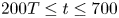 $200T\leq t\leq 700$. (c) The temporal mean
  $\langle \hat {\mathsf{{C}}}\rangle _t$ taken over
  $330T\leq t\leq 2200$.
Finally, the effect of both periodicity and artificial diffusivity on the elastic turbulence regime are directly assessed through examination of the temporal power law spectrum of velocity fluctuations, 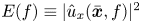 $E(f) \equiv |\hat {u}_x(\bar {\boldsymbol {x}},f)|^{2}$, where
  $\hat {u}_x$ represents the FFT of the velocity fluctuation,
  $u_x(\bar {\boldsymbol {x}},t^{*}) - \langle u_x(\bar {\boldsymbol {x}})\rangle _{t^{*}}$, for
  $t^{*}\in t$ in the statistically homogeneous regime at the position
  $\bar {\boldsymbol {x}}=(11{\rm \pi} /8,11{\rm \pi} /8)$ (figures 11 and 12). Notably, a fairly steep slope is a key characteristic of elastic turbulence (Groisman & Steinberg Reference Groisman and Steinberg2000, Reference Groisman and Steinberg2004; Steinberg Reference Steinberg2021). At a moderate level of artificial diffusivity (
 $Sc =1000$), figure 11 clearly shows that cases with
  $n\gneq 1$ levels of periodicity all conform to the same steep power law scaling behaviour, characteristic of elastic turbulence, whereas the R4 case (
 $n=1$) is clearly constrained to a lower range of frequencies, showing no apparent power law scaling behaviour. Notably, an exponent of
  $E\propto f^{-5.36}$ for the cases with
  $n\gneq 1$ level of periodicity is steeper than previous numerically (Berti et al. Reference Berti, Bistagnino, Boffetta, Celani and Musacchio2008; Gupta & Vincenzi Reference Gupta and Vincenzi2019) and experimentally (Groisman & Steinberg Reference Groisman and Steinberg2000, Reference Groisman and Steinberg2004; Sousa, Pinho & Alves Reference Sousa, Pinho and Alves2018) recorded values for elastic turbulence, and is largely attributed to the high level of artificial diffusivity imposed, which has been shown by Gupta & Vincenzi (Reference Gupta and Vincenzi2019) to increase the decay rate. To investigate the combined effects of artificial diffusivity and periodicity further, the spectral behaviour for the R4 and R16 cases was examined at
  $Sc =500$,
  $Sc =1000$ and
  $Sc =2000$ (figure 12). At high levels of artificial diffusivity (
 $Sc =500$), figure 12 shows that the R4 case (a) and R16 case (d) are constrained to low-frequency velocity fluctuations. This behaviour is largely expected given the high level of artificial diffusivity, which damps the high-wavenumber fluctuations of the polymer feedback (Gupta & Vincenzi Reference Gupta and Vincenzi2019). Despite this, the effect of periodicity on the problem is clearly noticeable, as the R4 case is clearly governed by strong periodic dynamics, whereas the velocity fluctuations for the R16 case are dispersed across a broader range of frequencies, illustrating a power law scaling behaviour
  $E\propto f^{-4.32}$. Further decreasing the level of artificial diffusivity, especially corresponding to
  $Sc =2000$ (figures 12c and 12f), unsurprisingly, allows both cases to sustain velocity fluctuations at much smaller scales. However, when comparing the effect of periodicity on the problem, it is clearly noticeable that both the R4 and R16 cases behave differently. More specifically, despite fluctuating across a broader range of frequencies at lower artificial diffusivity, the R4 case fails to follow any apparent power law scaling behaviour. On the other hand, the velocity fluctuations for the R16 case at
  $Sc =2000$ (figure 12f) behave as a fairly steep power law scaling
  $E\propto f^{-3.12}$, which is similar to previous experimental and numerical investigations of elastic turbulence with different forcings, in which the decay rate varied with the setup but the exponent was always smaller than
  $-3$ (Groisman & Steinberg Reference Groisman and Steinberg2000, Reference Groisman and Steinberg2001, Reference Groisman and Steinberg2004; Berti et al. Reference Berti, Bistagnino, Boffetta, Celani and Musacchio2008; Sousa et al. Reference Sousa, Pinho and Alves2018; Steinberg Reference Steinberg2021). As discussed, the exponent of
  $f^{-5.36}$ for the R16 case at
  $Sc =1000$ is a lot steeper, and is largely attributed to the higher level of artificial diffusivity (Gupta & Vincenzi Reference Gupta and Vincenzi2019). Nevertheless, the cases with
  $n\gneq 1$ levels of periodicity at
  $Sc =1000$ are able to retain and conform to the same steep power law scaling behaviour, characteristic of elastic turbulence, whereas the R4 case (
 $n=1$) is clearly constrained to a lower range of frequencies, showing no apparent power law scaling behaviour. The results are significant in not only highlighting the current misconception within the community for the standard four-roll mill problem with
  $n=1$ level periodicity as an elastic turbulence benchmark case (e.g. Thomases et al. (Reference Thomases, Shelley and Thiffeault2011), Gutierrez-Castillo & Thomases (Reference Gutierrez-Castillo and Thomases2019), Gupta & Vincenzi (Reference Gupta and Vincenzi2019), to a name a few), but also suggest that for certain problems, a finite level of artificial stress diffusivity (i.e.
  $Sc \neq \infty$) is still able to retain most of the characteristic features of elastic turbulence, given that the level of periodicity sufficiently retains the symmetry.

Figure 11. The temporal power spectral density  $E(f)$ of the velocity fluctuations for the R16 (red), R36 (blue) and R64 (green) cases at
  $Wi=10$ and
  $Sc =1000$. Note, all higher-periodicity cases (
 $n\gneq 1$) follow a power law,
  $E\propto f^{-5.36}$, behaviour. The inset corresponds to the spectral plot for the R4 case, which fails to follow a power law behaviour.

Figure 12. The temporal power spectral density  $E(f)$ of the velocity fluctuations at
  $Wi=10$ for the R4 case at Schmidt numbers (a)
  $Sc =500$, (b)
  $Sc =1000$ and (c)
  $Sc =2000$, and the R16 case at Schmidt numbers (d)
  $Sc =500$, (e)
  $Sc =1000$ and (f)
  $Sc =2000$. Note, all R4 cases fail to follow a power law scaling behaviour, whereas the R16 cases at
  $Sc =500$,
  $Sc =1000$ and
  $Sc =2000$ behave as a power law
  $E\propto f^{-4.32}$,
  $f^{-5.36}$ and
  $f^{-3.12}$, respectively.
4. Conclusions
To numerically simulate the complex dynamics of elastic turbulence most numerical studies rely on simplifications. This includes the addition of a global artificial diffusivity to overcome numerical stability issues that arise from steep polymer stress gradients and the use of PBCs to emulate an infinite system, such as benchmarks that rely on rotating and counter-rotating cylinder arrays to drive the elastic instabilities. In the inertialess limit the artificial diffusivity is known to adversely render the physical problem (Gupta & Vincenzi Reference Gupta and Vincenzi2019). In what has been believed to conserve unicity, numerical benchmarks with PBCs have largely investigated elastic turbulence with limited periodicity, i.e. using a single periodic image (unit cell), such as the popular four-roll mill benchmark using only four cylinders as the background force (Thomases & Shelley Reference Thomases and Shelley2009). In this work, we study the effect of PBCs including global artificial diffusivity on the four-roll mill benchmark case in the elastic turbulence regime. More specifically, we compared two-dimensional simulations with PBCs for the R4, R16, R36 and R64 cases using the Oldroyd-B model constitutive.
The present study finds that at the initial onset of viscoelastic instabilities for all levels of periodicity, the flow experiences a breakdown in initial symmetry, which eventually leads to the formation of a leading vortex. This initial flow asymmetry is consistent with the results obtained for the four-roll mill by Thomases & Shelley (Reference Thomases and Shelley2009) and Thomases et al. (Reference Thomases, Shelley and Thiffeault2011) and is attributed to the imposed artificial diffusivity (Gupta & Vincenzi Reference Gupta and Vincenzi2019). Beyond this initial breakdown in symmetry, the dominant presence of the single leading vortex within the single unit cell of the R4 case imposes quasi-periodic dynamics, as the system is unable to recover the initial symmetry with the vortex cycling around all four quadrants throughout time. In contrast, increasing the level of periodicity leads to a different behaviour, where the R16, R36 and R64 cases quickly overcome the effects of the single leading vortex, partially recovering the background forcing symmetry. In fact, it can be seen that the time taken to overcome the single leading vortex asymmetry and partly recover the initial roller effects decreases with each level of increasing periodicity, leading to a converging trend. The dynamics of the system with higher periodicity within this regime are purely chaotic, as the flow experiences high-frequency fluctuations that contribute to a broad range of temporal scales, as well as a fairly steep power law spectrum, which is consistent with previous numerical and experimental studies of elastic turbulence (Groisman & Steinberg Reference Groisman and Steinberg2000, Reference Groisman and Steinberg2001; Berti et al. Reference Berti, Bistagnino, Boffetta, Celani and Musacchio2008; Alves et al. Reference Alves, Oliveira and Pinho2021; Steinberg Reference Steinberg2021). Most notably, the combined unphysical effects of artificial diffusivity and finite periodicity were observed in the temporal power spectral density plots for the velocity fluctuations, which showed that high levels of artificial diffusivity ( $Sc=500$) suppressed the high-wavenumber fluctuations of the polymer feedback for both the R4 and R16 cases, consistent with the results obtained by Gupta & Vincenzi (Reference Gupta and Vincenzi2019). Upon decreasing the level of artificial diffusivity (
 $Sc=1000$ and
  $Sc=2000$), both cases retain a broader range of frequencies. However, the R4 case fails to follow any apparent power law scaling behaviour. On the other hand, the velocity fluctuations for the R16 case are characterised by a fairly steep power law scale. Whereby, higher levels of artificial diffusivity (
 $Sc=1000$) increase the decay rate of velocity fluctuations. Nevertheless, at this level of artificial diffusivity (
 $Sc=1000$), cases with
  $n\gneq 1$ all conform to the same power scaling behaviour. The results are significant in not only highlighting the current misconception within the community for the standard four-roll mill problem with
  $n=1$ level periodicity as an elastic turbulence benchmark case, but also suggest that for certain problems, a finite level of artificial diffusivity (i.e.
  $Sc \neq \infty$) is still able to retain most of the characteristic features of elastic turbulence, given that the level of periodicity sufficiently retains the symmetry.
Despite the increased chaotic nature of the flow, the R16, R36 and R64 cases are able to reduce the numerical artifacts due to global artificial diffusivity, as the polymer molecules are mostly stretched in the strain-dominated regions of the flow. This difference in behaviour between the different levels of periodicity at  $Wi=10$ was not limited to the specific level of elastic effects. When directly comparing the R4 and R16 cases across different
  $Wi$ numbers, it was found that the R4 regime transitioned from quasi-periodic (
 $Wi=10$) to fully periodic (
 $Wi=15$) and then to aperiodic dynamics (
 $Wi=20$), as originally observed by Thomases et al. (Reference Thomases, Shelley and Thiffeault2011). On the other hand, the R16 case does not experience such a broad range of dynamics, transitioning to a chaotic regime instantly at
  $Wi\approx 6.5$. It was shown through additional simulations of the R8 case (see Appendix B) that the numerical discrepancy observed for the R4 case is associated with the double PBCs of the system, as opposed to simply increasing the periodicity in one direction. In fact, the present results showed a moderate converging trend in recovering the symmetry of the flow with increasing levels of periodicity. Analogous simulations for the FENE-P constitutive model were performed (see Appendix A), showing similar results; hence, the effect of PBCs is not modified by the nonlinearity of the elastic force. Our results show that, combined with global artificial diffusivity, the consequence of PBCs can be dramatic if periodicity is insufficient. A theoretical analysis of this effect should be targeted in future work, notably by the derivation of an Ewald sum, which has enabled such a study on PBCs in periodic arrays of microswimmers (De Graaf & Stenhammar Reference De Graaf and Stenhammar2017). Overall, the current study finds that PBCs of the popular four-roll mill benchmark have a dramatic effect on the elastic turbulence regime, which can lead to unphysical behaviour, especially when combined with the effects from global artificial diffusivity. Although these unphysical qualities were shown to be reduced by increasing the level of periodicity, resembling certain features of non-diffusive solutions, the ability to retain the exact polymer representation is unmatched with the true solutions obtained by Gupta & Vincenzi (Reference Gupta and Vincenzi2019). In this respect, the current study highlights the previous misconceptions regarding the standard four-roll mill problem, using PBCs over a single unit cell, as an elastic turbulence benchmark, while also demonstrating the importance and caution required when applying PBCs in elastic turbulence problems combined with the effects of global artificial diffusivity.
Supplementary material and movies
Supplementary material and movies are available at https://doi.org/10.1017/jfm.2022.103.
Acknowledgements
The authors acknowledge the High-Performance Computing facilities at QUT and thank the QUT-HPC team for their support. V. Dzanic gratefully acknowledges QUT for support through a Ph.D. scholarship. The authors thank the anonymous reviewers whose feedback contributed to the overall improvement of the final manuscript.
Funding
A/Professor E. Sauret is the recipient of an Australian Research Council Future Fellowship (FT200100446) funded by the Australian Government.
Declaration of interests
The authors report no conflict of interest.
Appendix A. Effect of periodicity using the FENE-P model
A numerical limitation of the constitutive Oldroyd-B model is the unphysical unbounded molecular elongation of the polymer molecules. In this appendix, we perform analogous simulations using the FENE-P model, which imposes a maximum finite extensibility length for the polymer molecules:
 \begin{gather} \boldsymbol{\sigma}_p=f(r)\frac{\mu_p}{\tau_p} ({\boldsymbol{\mathsf{C}}}-{\boldsymbol{\mathsf{I}}}), \end{gather}
 \begin{gather}\frac{\partial{\boldsymbol{\mathsf{C}}}}{\partial t}+\boldsymbol{u}\boldsymbol{\cdot}\boldsymbol{\nabla} {\boldsymbol{\mathsf{C}}}={\boldsymbol{\mathsf{C}}}\boldsymbol{\cdot}(\boldsymbol{\nabla}\boldsymbol{u})+ (\boldsymbol{\nabla}\boldsymbol{u})^{\mathrm{T}}\boldsymbol{\cdot} {\boldsymbol{\mathsf{C}}}- \frac{f(r)}{\tau_p}({\boldsymbol{\mathsf{C}}}-{\boldsymbol{\mathsf{I}}}) +\kappa\boldsymbol{{\rm \Delta}}{\boldsymbol{\mathsf{C}}}. \end{gather}
The additional term,  $f(r)$, is used to impose a finite extensibility for the polymer molecules. The Oldroyd-B model (2.2) exhibits unbounded elongation
  $f(r)=1$ whereas the FENE-P model restricts the polymer elongation to a maximum length,
  $L$, such that
  $f(r)=({L^{2}-3})/({L^{2}-r^{2}})$ (Peterlin Reference Peterlin1961). Whereby,
  $r^{2}=\mathrm {tr}({\boldsymbol{\mathsf{C}}})$, which gives rise to a nonlinear spring force that diverges as
  $r^{2}\rightarrow L$, ensuring the dumbbell spring cannot extend beyond
  $L$ (Vaithianathan & Collins Reference Vaithianathan and Collins2003). The results for the additional simulations are shown for the vorticity contour (figure 13), polymer trace contour (figure 14) and the time series of the first component of the conformation tensor (figure 15). The additional results obtained using the FENE-P model are analogous to the results obtained using the Oldroyd-B model; hence, the effect of periodicity is not modified by the nonlinearity of the elastic force.

Figure 13. Contour plots for the vorticity field taken at the late stages corresponding to  $t=1300T$ for the (a) R4 case and (b) R16 case at
  $Wi=10$ using the FENE-P model.

Figure 14. Contour plots for the polymer trace field  $\mathrm {tr}({\boldsymbol{\mathsf{C}}})$ field taken at the late stages corresponding to
  $t=1300T$ for the (a) R4 case and (b) R16 case at
  $Wi=10$ using the FENE-P model.

Figure 15. Time series of the first component of the conformation tensor  $\mathsf{{C}}_{xx}$ at the position
  $[{\rm \pi},{\rm \pi} ]$ taken over the late stages of the flow for the R4 case (black) and R16 case (red) using the FENE-P model at
  $Wi=10$.
Appendix B. Effect of single PBCs using the R8 case
In this appendix, we report simulations conducted for an additional case for the four-roll mill, whereby the level of periodicity is only extended along a single direction, thus resulting in an eight-roll case, denoted R8. The results for the additional simulation are shown for the vorticity contour (figure 16), polymer trace contour (figure 17), and the time series of the first of the conformation tensor (figure 18).

Figure 16. Contour plot for the vorticity field taken at the late stages corresponding to  $t=1300T$ for the R8 case at
  $Wi=10$.

Figure 17. Contour plot for the polymer trace field tr $({\boldsymbol{\mathsf{C}}})$ taken at the late stages corresponding to
  $t=1300T$ for the R8 case at
  $Wi=10$.

Figure 18. Time series of the first component of the conformation tensor  $\mathsf{{C}}_{xx}$ at the position
  $[{\rm \pi},{\rm \pi} ]$ taken over
  $0\leq t/T \leq 3500$ for the R8 case at
  $Wi=10$.
The results for the additional R8 case show that increasing the level of periodicity in only one direction leads to the same leading-vortex structure observed for the R4 case. Both of these dominant vortices cycle around the quadrants over time, which numerically imposes quasi-periodic dynamics into the later stages of the flow, as shown in figure 18. Note, although the late-time dynamics observed for the R8 case in figure 18 are slightly different to the R4 case (refer to figure 5), the large-scale dynamics of the system are still governed by a quasi-periodic state.
Appendix C. Effect of periodicity in the hydrodynamic field
In this appendix, we show that the different dynamics observed for the different levels of periodicity are not specific to the polymer field. Additional results are shown for the hydrodynamic field, which compares the time series of the axial velocity at the location  $[11{\rm \pi} /8,11{\rm \pi} /8]$ for the R4, R16, R36 and R64 cases (figure 19). The results are analogous to the behaviour observed for the polymer field, whereby the chaotic regime for the R4 case experiences slow oscillations which transition into a quasi-periodic state, whereas the cases with higher levels of periodicity experience a purely chaotic behaviour.

Figure 19. Time series of the axial velocity  $u_{x}$ at the position
  $[11{\rm \pi} /8,11{\rm \pi} /8]$ taken over
  $400\leq t/T \leq 2500$. Results are compared at different levels of periodicity, namely, the (a) R4 (black), (b) R16 (red), (c) R36 (blue) and (d) R64 (green) case at
  $Wi=10$.


 Open access