


1. Introduction
The Richtmyer–Meshkov (RM) instability (Richtmyer Reference Richtmyer1960; Meshkov Reference Meshkov1969) is driven by the baroclinic generation of vorticity resulting from the misalignment of density and pressure gradients when a density-stratified interface is impulsively accelerated by a shock wave. The instability has gained significant scientific attention due to its relevance in supernovae explosions and applications in inertial confinement fusion (ICF) in finding a viable fusion-based energy source.
The RM instability can be viewed as a form of Rayleigh–Taylor (RT) instability (Taylor Reference Taylor1950) in the weak shock limit where the impulsive force is gravitational. Richtmyer (Reference Richtmyer1960) identified the similarities a decade later to formulate the linear stability theory for RM flows where the perturbation amplitude grows linearly until becoming comparable to its wavelength. The linear-amplitude growth rate for a sinusoidal (single-mode) perturbation between two fluids of different densities ( $\rho _1$, $\rho _2$) is given by
 \begin{equation} \dot{a} = kAVa_0, \end{equation}
where  $a_0$ is the initial amplitude, $k = 2 {\rm \pi}/ \lambda$ is the wavenumber, $V$ is the interface velocity and $A = {(\rho _2 - \rho _1)}/{(\rho _2 +\rho _1)}$ is the Atwood number. While some experiments (Aleshin et al. Reference Aleshin, Gamalii, Zaitsev, Lazareva, Lebo and Rozanov1988; Vassilenko et al. Reference Vassilenko, Buryakov, Kuropatenko, Olkhovskaya, Ratnikov, Jakovlev, Dannevik, Buckingham and Leith1992) have been able to verify the linear stability RM theory, others (Meshkov Reference Meshkov1969; Benjamin Reference Benjamin1988) have obtained notably lower growth rates. The disagreement has been attributed to nonlinearities induced by relatively large initial-amplitude conditions (Dimonte & Ramaprabhu Reference Dimonte and Ramaprabhu2010) or possibly, the effect of membrane strength (Jones & Jacobs Reference Jones and Jacobs1997) which may inhibit the initial development of the RM instability from not being able break down into sufficiently small scales. As the amplitude and wavelength become comparable, nonlinear mechanisms cause perturbations to grow as asymmetrical bubbles and spikes and cause a reduction in growth rate.
The most common method employed in laboratory tests studying the RM instability is to study the passage of a shock wave across a perturbed boundary between two gases. The main hurdle occurs in forming a well-defined interface between the two gases (Jones & Jacobs Reference Jones and Jacobs1997) by methods that do not affect the post-shock flow. Such an issue does not occur in liquid systems, however, the scale of forces associated with these explosively driven experiments (Benjamin Reference Benjamin1988) poses a much larger safety concern with high operation costs and large preparation times. Most experiments therefore, starting from the earliest work of Meshkov (Reference Meshkov1969, Reference Meshkov1970) and his co-workers (Aleshin et al. Reference Aleshin, Gamalii, Zaitsev, Lazareva, Lebo and Rozanov1988; Vassilenko et al. Reference Vassilenko, Buryakov, Kuropatenko, Olkhovskaya, Ratnikov, Jakovlev, Dannevik, Buckingham and Leith1992; Andronov et al. Reference Andronov, Zhidov, Meshkov, Nevmerzhitskii, Nikiforov, Razin, Rogatchev, Tolshmyakov and Yanilkin1995) have resorted to gas systems that used a thin sinusoidal nitrocellulose membrane to separate the gases and set up the initial perturbation. While the membrane was shattered by the incident shock wave, the fragment pieces produced were carried with the ensuing flow and affected the late-time development of the RM instability significantly (Jones & Jacobs Reference Jones and Jacobs1997). More recent studies (Prasad et al. Reference Prasad, Rasheed, Kumar and Sturtevant2000; Jourdan & Houas Reference Jourdan and Houas2005) have employed a wire mesh to support the thin nitrocellulose membrane. In this scenario, while the membrane suppresses mixing by isolating the two gases from each other and retarding motions due its inertia and the viscous no-slip condition, the wire mesh enhances mixing by slicing the membrane into ribbons and producing wake-generated turbulence. This can make studying the effect of initial conditions on perturbation growth difficult. The membrane fragments also impede the use of advanced visualization techniques such as particle image velocimetry (Prestridge et al. Reference Prestridge, Rightley, Vorobieff, Benjamin and Kurnit2000), planar laser-induced florescence (Jacobs et al. Reference Jacobs, Klein, Jenkins and Benjamin1993; Rightley et al. Reference Rightley, Vorobieff, Martin and Benjamin1999) and planar Rayleigh scattering (Budzinski, Benjamin & Jacobs Reference Budzinski, Benjamin and Jacobs1994).
The interface can also be formed by withdrawing a thin plate separating the two fluids (Cavailler et al. Reference Cavailler, Mercier, Rodriguez and Hass1990; Brouillette & Sturtevant Reference Brouillette and Sturtevant1994; Bonazza & Sturtevant Reference Bonazza and Sturtevant1996; Puranik et al. Reference Puranik, Oakley, Andersen and Bonazza2004). The withdrawing motion, however, creates a boundary layer due to the no-slip condition. This drags a volume of fluid along the plate surface which bounces back off shock tube walls to form surface gravity waves once the plate is completely removed from the test section (Bonazza & Sturtevant Reference Bonazza and Sturtevant1996; Zhou Reference Zhou2017). In addition, the RT instability begins developing immediately as soon as the two gases (if the heavier one is above) come into contact when the plate begins sliding out (Puranik et al. Reference Puranik, Oakley, Andersen and Bonazza2004). The interface produced in this manner is very diffuse ( $>$1 cm) which can reduce the RM instability growth rate significantly (Mikaelian Reference Mikaelian1991; Jones & Jacobs Reference Jones and Jacobs1997; Collins & Jacobs Reference Collins and Jacobs2002; Morgan, Likhachev & Jacobs Reference Morgan, Likhachev and Jacobs2016). While Puranik et al.'s (Reference Puranik, Oakley, Andersen and Bonazza2004) study was the only work to use a sinusoidally shaped plate, the initial perturbation induced in earlier studies was solely dependent on the disturbance created by the sliding motion of the flat plate. Thus, although initial conditions in both cases were subjective to plate retraction, the latter suffered appreciably more with non-sinusoidal perturbations which were difficult to characterize and be used for comparison purposes. The plate retraction method allowed Puranik et al. (Reference Puranik, Oakley, Andersen and Bonazza2004) to study particularly large initial amplitudes ( $ka_0 = 1.46$) in the heavy/light configuration, however, dispersion of stable Rayleigh–Taylor oscillations in light/heavy set-up caused the interfacial perturbations to flatten out almost immediately.
Other methods to solve the interface generation problem involve gently oscillating the shock tube at an appropriate frequency using a stepper motor and crank mechanism to generate standing waves at the interface location (Jones & Jacobs Reference Jones and Jacobs1997; Collins & Jacobs Reference Collins and Jacobs2002; Jacobs & Krivets Reference Jacobs and Krivets2005; Morgan et al. Reference Morgan, Aure, Stockero, Greenough, Cabot, Likhachev and Jacobs2012). While this method produced particularly well-defined initial perturbations ( $ka_0 \approx 0.16\text {--}0.34$), excessively large shock tube oscillations resulted in an asymmetrical interface. The technique, nevertheless, shows good promise but extreme oscillatory measures to achieve large $ka_0$ initial conditions ( $>$0.5) may add complications with the use of fixed optical diagnostic systems and heavy/large shock tubes. This issue is being addressed by localizing the oscillatory motion using pistons movements at the interface (Motl et al. Reference Motl, Niederhaus, Ranjan, Oakley, Anderson and Bonazza2007) where a stepper motor oscillates the pistons laterally at a given frequency to develop a standing wave. Interface reproducibility and controllability using this method, however, still need to be investigated. Jacobs et al. (Reference Jacobs, Krivets, Tsiklashvili and Likhachev2013) induced vertical oscillations in the gas column by using two out-of-phase loudspeakers attached to the top and bottom of the shock tube. This creates Faraday waves at the interface which are associated with small random three-dimensional perturbations.
More recently, a soap-film technique to form gaseous interfaces with a well-characterized discontinuous configuration was developed (Liu et al. Reference Liu, Liang, Ding, Liu and Luo2018). The interfacial morphology captured by this method was physically superior to past membrane and membraneless techniques producing clear roll-up structures uninfluenced by either fragment pieces or the presence of a diffuse interface layer, respectively. The test section used, however, was relatively narrow (7 mm), possibly due to soap-film formation limitations which can lead to wall effects at late times. Lastly, the counterpart of corrugated interfaces interacting with a planar shock wave, i.e. a non-uniform shock-wave deposition on a flat interface to generate the RM instability, has also been explored. A planar shock diffracting around a rigid cylinder as such can be used to produce a rippled shock wave (Zou et al. Reference Zou, Liu, Liao, Zheng, Zhai and Luo2017) resulting in a ‘ $\bigwedge$’ shaped interface and a cavity after colliding with a uniform interface.
Given the problems associated with interface generation in gas systems, we develop a novel yet simple method where the undulating motion of a cross-flow is used to set up the initial conditions. An airfoil flapper upstream from the test section is used to oscillate the cross-flow at pre-set frequencies and amplitudes. The technique allows us to produce near-sinusoidal perturbations with a dominant mode for a large range of  $\overline {ka_0}$ values (0.30–0.86). Thus, we determine the effect of systematically increasing initial perturbation wavelengths and amplitudes on the growth and mixing transition of the RM instability. The perturbation growths are compared with previous nonlinear models and simulations to ascertain their initial condition dependence. Velocity field measurements from planar particle image velocimetry are used for vortex identification and obtaining turbulent statistics to describe the temporal evolution of the flow. The separation of energy containing and dissipative scales along with the local and global flow characteristics are then used to determine the effect of initial conditions on mixing transition with particular emphasis on the transition criterion used.
2. Experimental facility
All experiments are conducted at the Los Alamos National Laboratory (LANL) Vertical Shock Tube (VST) facility (figure 1a). A diaphragmless plug and sleeve two-piston driver (Mejia-Alvarez et al. Reference Mejia-Alvarez, Wilson, Leftwich, Martinez and Prestridge2015) is used to produce a Mach 1.2 planar shock wave in a 7 m tall  $127~\textrm {mm}\times 127~\textrm {mm}$ square cross-section shock tube. The VST consists of three diagnostic stations (figure 1b). A close-up of station 1 ( $x = 0$ cm) is given in figure 1(c) while stations 2 and 3 are situated at $x = 28$ and 63 cm downstream. Air is bulk filled from the top and SF $_6$ from the bottom until the two gases meet and start exiting through the outlet on the left at station 1 ( $A \sim 0.67$). This creates a stagnation point flow at the interfacial location that has the added effect of thinning the diffusion layer. The air (upper side inlet) and SF $_{6}$ (lower side inlet) cross-flow is first streamlined individually by passing through a two-part honeycomb mesh. Flapper oscillations at the mesh exit then produces an undulating cross co-flow that enters the test section at 0.2 m s $^{-1}$ (from right-to-left) through a $12.70~\textrm {cm} \times 3.81~\textrm {cm}$ channel to form a perturbed interface. The cross-flow is vented out from the exhaust opposite to the inflow to prevent any accumulation within the shock tube from causing unwanted disruptions to the interface. The steady-state flapper oscillation frequency and total rotation angle used ranged between 0.25 and 3 Hz and $8$ to $16^\circ$.

Figure 1. Schematic of the experimental set-up. (a) Overview of the 7 m tall vertical shock tube (VST). The shock is generated downwards by a pneumatic piston situated at the top end. (b) Optical diagnostics at stations 1–3 numbered in shock travel direction. Station 1 particle image velocimetry laser sheet is produced vertically from the base of the VST while those for station 2 and 3 traverse horizontally. (c) Close-up overview of the initial condition interface set-up at station 1. Flapper oscillations produce a perturbed interface.
When the driver is depressurized to generate a shock wave, two pneumatically driven gates close the inlet and outlet at each end of the test section (see figure 1). This prevents effects from sidewall openings that can weaken the incident shock wave, introduce non-uniformities and also damage the flapper mechanism. Although one can expect a stagnation point flow to form briefly (until the shock arrives,  ${\rm \Delta} t \approx 0.1$ s) from blocking the cross-flow at the left gate and in turn cause near-wall jetting on the opposite end, the flow disruption created is minor in comparison to gas purging following shock passage if the cross-flow slots are left open. The shock location is monitored using six pressure transducers as it travels down the tube from the driver. The pressure signals are also used to trigger the optical diagnostic systems at each station. All operations including timing, servo-motors, test section gates, flapper, shock driver, gas flows and diagnostics are controlled using LabVIEW.
A single image taken at station 1 just prior to the arrival of the shock wave ( $t=0$ ms) is used to record the initial conditions while two-dimensional particle image velocimetry (PIV) diagnostics capture a pair (7 $\mathrm {\mu }$s interframe delay) to image the ensuing structures at stations 2 and 3. Nd:YAG lasers operating at 532 nm wavelength are used for PIV measurements, and the flow is seeded with olive oil particles (mixed with SF $_6$ bulk and cross-flow using a Laskin nozzle). An optical train (spherical lens followed by cylindrical lens) is used to shape the laser beam into a thin diverging light sheet and directed into the shock tube longitudinally, using a $45^\circ$ angled mirror at the bottom for station 1 and laterally from sides at stations 2 and 3. The flow fields are visualized at each station using a TSI PowerView camera having a $4008 \times 2672$ charged couple device array. The image pairs are processed using a 3-pass recursive Robust Phase Correlation algorithm (Eckstein & Vlachos Reference Eckstein and Vlachos2009) in the PRANA (PIV, Research and ANAlysis) software (https://github.com/aether-lab/prana) with a final window size of $32 \times 32$ pixels at 50 % overlap which translated to a 464 $\mathrm {\mu }$m vector spacing.
2.1. Interface characterization
Characterizing the interface for each flapper condition is crucial given the objective of this study to determine the effect of initial conditions on the late-time development of the RM instability. Three different sets of initial conditions are investigated using a combination of oscillating plate frequencies,  $f$ (Hz), and sweeping angles, $\sphericalangle$ (
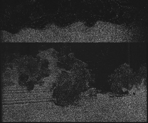
 $^\circ$), (see table 1). Figure 2 (top row) shows initial interface images for (a) 0.25 Hz, 8 $^\circ$, (b) 3 Hz, 8 $^\circ$ and (c) 3 Hz, 16 $^\circ$. The interface has a spectrum of residual small-amplitude short-wavelength perturbations (Vandenboomgaerde et al. Reference Vandenboomgaerde, Souffland, Mariani, Biamino, Jourdan and Houas2014) and is not perfectly sinusoidal as in the case of a pure single-mode instability, especially for larger flapper frequencies and sweeping angles, where the asymmetric and multi-modal features are more pronounced. However, a dominant wavelength and amplitude are still noticeable. Although the RM-instability initially follows a linear growth rate, the dominant mode quickly dominates the flow (Morgan et al. Reference Morgan, Aure, Stockero, Greenough, Cabot, Likhachev and Jacobs2012) once nonlinearities set in as the perturbation wavelength and amplitude become comparable.
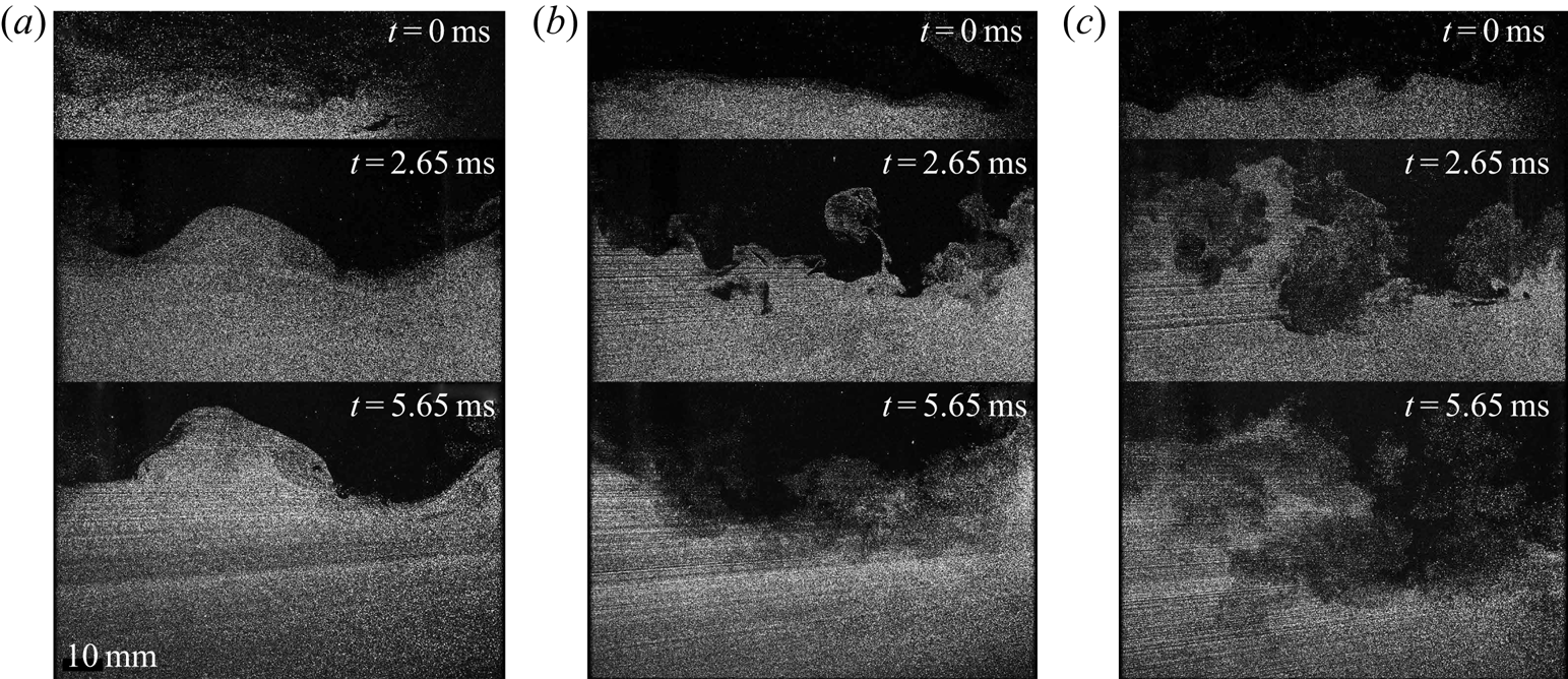
Figure 2. Initial condition ( $t=0$ ms) and ensuing structures at $t=2.65$ and 5.65 ms for $\overline {ka_{0}}= (a)\ 0.3, (b)\ 0.53$ and (c) 0.86. The cross-flow direction in the initial conditions is from right to left.
Table 1. Flapper oscillation parameters and corresponding initial interface characteristics. Overbar symbols represent mean values with  $\pm$ as standard deviations.

We determine the interfacial location using an edge detection image processing routine in MATLAB. The initial conditions are extracted by fitting the perturbation with a cubic spline (Epps, Truscott & Techet Reference Epps, Truscott and Techet2010) and computing its first and second derivatives to obtain the crest and trough locations. Obtaining the initial amplitudes and wavelengths from these measurements, we find average values for each experiment (Jacobs et al. Reference Jacobs, Krivets, Tsiklashvili and Likhachev2013) that are then ensemble averaged over eight realizations ( $\bar{a}_0$, $\bar {\lambda} _0$) for each flapper condition, with the corresponding variations (standard deviations) listed in table 1. All interface measurements are made at the instant just prior to shock impact ( $t=0$ ms). Competition between the size of the inlet slot, the size of the wake structure and the oscillatory displacement of the trailing flapper edge causes disproportionate reductions in the dominant perturbation wavelength for the higher flapper frequencies in table 1.
It is noteworthy that the spectrum of small-amplitude short-wavelength perturbations observed is inevitable in real-life experiments where the interface is machine made. In fact, it has been shown that running numerical simulations with the addition of such residual perturbations to single-mode interfaces is necessary to understand the morphology of the experimental picture (Vandenboomgaerde et al. Reference Vandenboomgaerde, Souffland, Mariani, Biamino, Jourdan and Houas2014). As such, the deviation in experiments herein from the ideal case of a pure single-mode perturbation allows us to complement single-mode work by improving them to be closer to reality.
3. Results
3.1. Mixing widths and scaling
Growth of the RM instability for increasing  $\overline {ka_0}$ initial conditions is shown in figure 2. The first image row shows the interface at ( $t=0$ ms) while the second and third rows are recorded at $t=2.65$ and 5.65 ms. Mixing transition, as observed by the breakdown of large-scale features into smaller structures, is faster for larger $\overline {ka_0}$. For low $\overline {ka_0}$, the dominant wavelength is preserved for the times measured, while rapid breakdown to smaller length scales is evident for $\overline {ka_0} = 0.53$ and 0.86 at $t = 5.65$ and 2.65 ms, respectively. The enhancement in mixing observed that eventually triggers a transition to turbulence can be related to secondary RM instabilities (Peng, Zabusky & Zhang Reference Peng, Zabusky and Zhang2003) following the primary baroclinic vorticity deposition. This secondary vorticity deposition dominates at intermediate times due to the misalignment of density gradient across the interface and vortex-centripetal acceleration arising from the large-scale rotation of coherent vortices formed by the primary vorticity roll-up. More explicitly, opposite-sign vorticities generated at the neck and arms of the mushroom structures are advected into the vortex core. This local fluid entrainment causes mixing and the structure to disintegrate accordingly.
Since the interface formed is not perfectly sinusoidal, the presence of a spectrum of residual small-amplitude short-wavelength perturbations (Vandenboomgaerde et al. Reference Vandenboomgaerde, Souffland, Mariani, Biamino, Jourdan and Houas2014) and multi-mode fronts observed can cause mode coupling (Rupert Reference Rupert1991) in the nonlinear late-time growth regime. Large scales develop by means of a bubble-competition mechanism (Zufiria Reference Zufiria1988) and vortex pairing. As each bubble tries to occupy the maximum possible space and compete with others, smaller bubbles advance less due to lower speeds (Layzer Reference Layzer1955). This causes them to shrink and slow down while larger ones expand and acquire higher vortex speeds. Eventually, bubbles overtake their smaller neighbours to form a larger bubble, also known as a ‘bubble merger’ (Sharp Reference Sharp1984; Glimm et al. Reference Glimm, Li, Menikoff, Sharp and Zhang1990). This imbalance in cross-coupling strengths may also induce a tilt effect on the interface which is likely to become prominent for higher  $\overline {ka_0}$ conditions due to increasing competition in less space. For example, a clockwise interface tilt at $t=5.65$ ms is noted for the highest $\overline {ka_0}$ in figure 2(c) due to slower growth near the right edge. This disturbs the evolution of some adjacent bubbles and spikes further from growing into each other. A similar tilting feature and disruption in mushroom structures was also noted in gas-curtain experiments (Orlicz, Balasubramanian & Prestridge Reference Orlicz, Balasubramanian and Prestridge2013) from disparities in counter-rotating vortex strengths.
The interface breaks up at late times to form mixing regions which then make it difficult to determine its shape. We define the mixing layer width  $h$ as the distance between 5 % and 95 % values of the average concentration profile with a mean amplitude, $a=h/2$. The images are first corrected for non-uniform illumination using morphological opening and adjusted background subtraction. Morphological opening using a disk-shaped structuring element of radius greater than the particle diameter allows us to obtain a background approximation image which can be subtracted from the original image to give uniform illumination. Spanwise averaging is then performed to obtain a mean olive oil concentration distribution. A typical normalized plot is shown in figure 3 where the distance between dashed lines is taken as the mixing width.

Figure 3. Normalized mean concentration distribution of olive oil particles with streamwise distance;  $\bar {Q}_{max}$ represents the maximum of the mean concentration profile. The dashed lines indicate 5 % and 95 % of the mean particle concentration ( $\overline {ka_0}=0.86$, $t= 2.65$ ms, $h=44$ mm).
Growth in mixing widths with downstream distance are shown in figure 4(a). As observed, higher  $\overline {ka_0}$ initial conditions result in larger growth with the increase being notably significant for the highest $\overline {ka_0}$. Normalizing the layer growth $(a-a_0)$ with wavenumber $k$ (Prasad et al. Reference Prasad, Rasheed, Kumar and Sturtevant2000) highlights the effect in terms of the non-dimensional amplitude (figure 4b). Power-law exponents from fits to the data are found to range between 0.35 and 0.37 for $\overline {ka_0}= 0.30\text {--}0.86$. An empirical relation that generalizes the growth of the studied initial conditions is
 \begin{equation} k \left( \frac{a}{a_0} \right)= 0.6(kx)^{0.36}, \end{equation}
where all lengths are in mm. The scaling is shown in figure 5.

Figure 4. (a) Effect of initial conditions on mixing widths with respect to downstream distance. Mean values at  $x \approx 280$ mm are $h\ (\textrm {mm}) = 31.3, 34.2, 47.1$ and at $x \approx 630$ mm are $h\ (\textrm {mm}) = 39.7, 43.3, 60.1$ for $\overline {ka_0} = 0.30, 0.53$ and 0.86 (see table 1 for details). (b) Dimensionless amplitude as a function of normalized distance. Power-law fits follow $k(a-a_0) \propto (kx)^n$ where $n = 0.37, 0.35, 0.36$, respectively.

Figure 5. Dimensional scaling  $k({a}/{a_{0}})=0.6(kx)^{0.36}$ yields minimum scatter for present data.
The late-time growth of the mixing zone has been suggested by a number of researchers (Mikaelian Reference Mikaelian1989; Alon et al. Reference Alon, Hecht, Ofer and Shvarts1995; Zhou Reference Zhou2017) to follow a power-law behaviour  $h \sim \tau _i^{\theta }$ where $\tau _i$ is a linear function of time, and the scaling exponent $0.2 \lesssim \theta \lesssim 0.6$ has been a subject of active research. Our generalized scaling exponent (0.36) is in good agreement with those of Jacobs et al. (Reference Jacobs, Krivets, Tsiklashvili and Likhachev2013) (0.3–0.4) and close to Weber et al. (Reference Weber, Haehn, Oakley, Rothamer and Bonazza2014) ( $0.43 \pm 0.01$), both of which used membraneless techniques to impose the initial conditions. Values by Krivets, Ferguson & Jacobs (Reference Krivets, Ferguson and Jacobs2017) varied over a large range (0.19–0.57) having ensemble averages of $\theta _b = 0.38$ and $\theta _s = 0.4$ for bubble and spike growth exponents, respectively. Laser-driven experiments by Dimonte & Schneider (Reference Dimonte and Schneider1997) found $\theta =0.5 \pm 0.1$ for $A \thicksim 0.9$. Later, Dimonte & Schneider (Reference Dimonte and Schneider2000) found bubbles and spike responses of $\theta _b = 0.25$ and $\theta _s = 0.3$ (for $A \thicksim 0.7$). However, to compensate for demixing caused by any residual deceleration in their linear electric motor system (Dimonte et al. Reference Dimonte, Morrison, Hulsey, Nelson, Weaver, Susoeff, Hawke, Schneider, Batteaux and Lee1996), it was suggested that these exponents may have to be increased by ${\thicksim }10\,\%$. Experiments performed using membranes by Prasad et al. (Reference Prasad, Rasheed, Kumar and Sturtevant2000) produced a late-time growth exponent of ( $0.26 \leq \theta \leq 0.33$). Although more experiments are needed to ascertain the influence of membranes on the growth rate, comparing our results with studies employing shock tube set-ups for similar shock strengths and Atwood numbers (Prasad et al. Reference Prasad, Rasheed, Kumar and Sturtevant2000; Jacobs et al. Reference Jacobs, Krivets, Tsiklashvili and Likhachev2013; Weber et al. Reference Weber, Haehn, Oakley, Rothamer and Bonazza2014; Krivets et al. Reference Krivets, Ferguson and Jacobs2017) indicates membrane remnants suppress the growth exponent $\theta$ in the light–heavy configuration on average by ${\sim }23\,\%$. This is similar to an average growth reduction of ${\sim } 27\,\%$ found in the nonlinear interfacial harmonics by Mariani et al. (Reference Mariani, Vandenboomgaerde, Jourdan, Souffland and Houas2008) using membranes in comparison to numerical and theoretical growth rates.
3.2. Evaluation of single-scale nonlinear models
Modelling the extension of the linear regime into the nonlinear growth phase has been attempted by a number of distinct studies and is a topic of active research in the RMI community. Among the methods employed for this purpose include using potential-flow models, heuristic/interpolation approaches, Padé approximants and numerical simulations solving the Euler conservation system in a hydrodynamic continuum. We provide a brief overview of these methods followed by a comparison with results from present experiments to propose a rational interpolation model that matches our late-time growth rates.
Layzer's potential-flow modelling approach (Layzer Reference Layzer1955) was the first to describe bubble evolution of the RT instability based on an approximate solution satisfying the equations of motion for a fluid particle in the vicinity of the bubble tip. The problem was initialized from a flat free-surface interface with a constant-pressure condition imposed at the bubble vertex and its immediate neighbourhood. Although Layzer's theory is limited to incompressible fluids having an infinite density ratio ( $A =1$), the approximate solutions presented for the vertex speed and its asymptotic form have served as a guideline in further understanding the evolution of RT and RM instabilities in different configurations. Generalizing Layzer's theory to non-zero initial bubble amplitudes and applying it to the RM instability, Mikaelian (Reference Mikaelian1998) obtained an analytical solution to capture the motion of the bubble vertex from the linear to the nonlinear regime. The solution for bubble amplitude, given as
 \begin{equation} a_b = \left[a_{0} k + ( \tfrac{2}{3} ) \ln (1+3 v_0 kt/2)\right]/k, \end{equation}
where  $v_0$ represents the initial velocity as $\dot {a}$ in (1.1), did not deviate from direct numerical simulation results by more than 10 % for $ka_0 = 1/6\text {--}2/3$. Since this analytical expression was limited to an infinite density ratio system (i.e. $A =1$), Mikaelian (Reference Mikaelian2003) generalized the solution to arbitrary $A$ by using a simple transformation found from analysing an extension of Layzer's theory to finite density ratios (Goncharov Reference Goncharov2002). The method essentially is to transition from a linear to nonlinear solution at a specific amplitude $a^*$, where the expression for the nonlinear two-dimensional (2-D) RM instability is given by
 \begin{equation} a_b = a^*+ \frac{(3+A)}{3(1+A)k}\ln\{1+3 v_0 k (t-t^*)(1+A)/(3+A)\} \end{equation}
with an asymptotic velocity  $v_b = {(3+A)}/[{3(1+A)kt}]$. More explicitly, $a_b$ was given by the linear regime until $t^* \equiv t_{M}^* = ({1}/{VkA}) ({1}/({3a_0k})-1)$ when $a^* \equiv a_{M}^* = {1}/{3k}$ after which it followed the generalized Layzer-type solution (3.3). Although only bubble growth was considered, it is possible to apply the transformation ( $\eta \rightarrow -\eta$, $A \rightarrow -A$) from Goncharov (Reference Goncharov2002) to obtain the asymptotic spike velocity as $v_s = {(3-A)}/[{3(1-A)kt}]$ (Jacobs & Krivets Reference Jacobs and Krivets2005). While the solution may not be appropriate when $ka_0> 1/3$, the evaluation of (3.3) for an extended $ka_0$ range is appealing due its simplistic nature. An alternate approach attributed to Enrico Fermi by Layzer (Reference Layzer1955) was also proposed where the linear regime lasted until the bubble growth rate became equal to its asymptotic velocity. The transition in this case occurred at $t^* \equiv t_{F}^* = {(3+A)}/[{3(1+A)k^2 VAa_0}]$ when $a^* \equiv a_{F}^* = a_{0} (1 + {(3+A)}/[{3(1+A)ka_0}])$. Since $t_F^* >t_M^*$ and $a_F^*>a_M^*$, the transition in the Mikaelian–Fermi model (Mikaelian Reference Mikaelian2003) ( $t^* \equiv t_F^*$, $a^*\equiv a_F^*$) occurred 2–3 times later than Mikaelian's (Reference Mikaelian2003) model ( $t^* \equiv t_M^*$, $a^*\equiv a_M^*$) resulting in comparatively larger amplitudes.
Zhang & Guo (Reference Zhang and Guo2016) considered Layzer's theory for incompressible, inviscid and irrotational fluids with arbitrary density ratios in two dimensions to study the asymptotic large-time behaviour of RT and RM instabilities. The property of both the velocity and curvature of the finger (both bubble and spike) tip being insensitive to time in the quasi-steady state was used to obtain an expression for the RT finger velocity which could then be simplified for the RM case by taking the limit  $g \rightarrow 0$ to produce a matched solution
 \begin{equation} v_{b/s} = \frac{v_0}{1+\alpha k v_0 t}, \end{equation}
where
 \begin{equation} \alpha = \frac{3}{4} \frac{(1 \pm A)(3 \pm A)}{[3 \pm A + \sqrt{2}(1\pm A)^{1/2} ]} \frac{4(3 \pm A)+\sqrt{2}(9 \pm A)(1 \pm A)^{1/2}}{[(3 \pm A)^2 + 2\sqrt{2}(3 \mp A)(1 \pm A)^{1/2}]}. \end{equation}
 More importantly, introducing scaled dimensionless variables  $u_{RM}={v}/{v_0}$ and $\tau _{RM} = \alpha k v_0 t$ was shown to describe all bubble and spike growth rates at any density ratio by a universal curve $u_{RM} = {1}/{(1+\tau _{RM})}$ until a pre-asymptotic stage.
Sadot et al. (Reference Sadot, Erez, Alon, Oron, Levin, Erez, Ben-Dor and Shvarts1998) formulated an empirical rational function with late-time behaviour functionality based on comparisons between experiments, numerical simulations and a simple potential-flow model for single-mode and two-bubble cases. The growth rate was proposed as
 \begin{equation} v_{b/s} = \frac{v_0(1+v_0 kt)}{1+ (1 \pm A)v_0 kt + E_{b/s} v_0^2 k^{2} t^{2}}, \end{equation}
where the term  $E_{b/s}=[(1 \pm A)/(1+A)](1/2{\rm \pi} C)$ becomes dominant as $t\rightarrow \infty$, $v_{b/s}= {1}/({E_{b/s}kt})$ (the plus sign being for the bubble and minus for spike) following the $1/t$ dependence obtained from potential-flow theory (Hecht, Alon & Shvarts Reference Hecht, Alon and Shvarts1994). The coefficient $C$ is thus a function of the asymptotic velocity which was suggested to follow $C={1}/({3 {\rm \pi}})$ for $A \gtrsim 0.5$ and $C = {1}/({2 {\rm \pi}})$ for $A \rightarrow 0$ to obtain convergence with their asymptotic limits. These values were chosen to match the simulation results of Alon et al. (Reference Alon, Hecht, Ofer and Shvarts1995) who obtained $E_b = 1.5$ for $A \gtrsim 0.5$ and $E_b \approx 1.06$ at low Atwood numbers. Asymptotic velocities obtained by Goncharov (Reference Goncharov2002) and Mikaelian (Reference Mikaelian2003) followed $E_{b/s} = {3(1 \pm A)}/({3 \pm A})$ while an extension of Layzer's theory for finite density ratios using different velocity potentials by Sohn (Reference Sohn2003) showed $E_{b/s} = ({2 \pm A})/{2}$. The buoyancy–drag model by Niederhaus & Jacobs (Reference Niederhaus and Jacobs2003) in contrast was used to propose $E_{b/s} = 1 \pm A$ as a modified form of Sadot et al.'s model. Despite the use of similar analytical procedures by Alon et al. (Reference Alon, Hecht, Ofer and Shvarts1995) and Niederhaus & Jacobs (Reference Niederhaus and Jacobs2003), the expressions for asymptotic velocities obtained were different. This can be attributed to the discrepancy in added mass effects employed in the two-dimensional bubble model. Although Sadot et al.'s (Reference Sadot, Erez, Alon, Oron, Levin, Erez, Ben-Dor and Shvarts1998) model captures both the $1/t$ long-time dependence and the weakly nonlinear solution, up to second order (Haan Reference Haan1991), the correct value of $C$ and the corresponding expression for $E$ at intermediate Atwood numbers remains uncertain (Collins & Jacobs Reference Collins and Jacobs2002; Jourdan & Houas Reference Jourdan and Houas2005).
The perturbation expansion method can be used to expand nonlinearities in terms of spatial harmonics with time-dependent amplitudes. Differentiating the leading harmonics (Zhang & Sohn Reference Zhang and Sohn1997a) with respect to time and collecting odd and even cosine Fourier modes at  $x = 0$ (for spikes) and ${\rm \pi} /k$ (for bubbles), leads to perturbations solutions in the form of truncated Taylor series in the amplitude of the initial perturbation. Since these solutions are divergent in nature, the radius of convergence of this expansion is very limited. In order to extend the range of approximation Zhang & Sohn (Reference Zhang and Sohn1997b) constructed a single-point Padé approximant, a ratio of two power series in $t$, where the bubble and spike growth rate were given by
 \begin{gather} v_{b/s} = v_1 \mp v_{2}, \end{gather}
 \begin{gather}v_1 \equiv \frac{v_0}{1+a_{0} v_0 k^{2}t + max\left\{0,a_{0}^2 k^2 - A^2 + \tfrac{1}{2}\right\}v_0^2 k^{2} t^{2}}, \end{gather}
 \begin{gather}v_2 \equiv \frac{A k v_0^2 t}{1+2k^2 a_0 v_0 t + 4k^2 v_0^2[a_0^2 k^2 + (1/3)(1-A^2)]t^2}. \end{gather}
Although the model has been shown to be in good agreement with experiments (Jacobs & Krivets Reference Jacobs and Krivets2005) and numerical simulations for linear and intermediate nonlinear stages, the small-time solution information used cannot capture the  $1/t$ asymptotic behaviour of the potential-flow theory as $t = \infty$. Another important issue using an average overall velocity $\bar {v} =(v_b + v_s)/2 \equiv v_1$ is the omission of the $v_2$ component which removes the contribution of even cosine Fourier modes.
Building upon models by Sadot et al. (Reference Sadot, Erez, Alon, Oron, Levin, Erez, Ben-Dor and Shvarts1998), Mikaelian (Reference Mikaelian1998, Reference Mikaelian2003) and Zhang & Sohn (Reference Zhang and Sohn1997b), Dimonte & Ramaprabhu (Reference Dimonte and Ramaprabhu2010) presented a nonlinear empirical model describing their 2-D FLASH code numerical simulations for a broad range of Atwood numbers and scaled initial amplitudes  $ka_0$. The model thus focused at more relevant conditions in ICF and ejecta formation applications where $A$ and $ka_0$ are large. The bubble and spike growth rates were given as
 \begin{equation} v_{b/s} = v_0 \frac{1+(1\mp|A|)\tau}{1+\left( \dfrac{4.5 \pm|A| +(2\mp|A|)|k a_0|}{4} \right)\!\tau +(1\mp|A|)(1\pm|A|)\tau^2}. \end{equation}
The simulations revealed spikes are very sensitive with respect to  $ka_0$ whereas bubbles are not. Long duration simulations further showed spike velocities to deviate from the $1/kt$ scaling as $|A| \rightarrow 1$, thus indicating their asymptotic non-universality.
Recalling Richtmyer's (Reference Richtmyer1960) findings, an impulsively accelerated sinusoidal perturbation in an incompressible system was shown follow a linear-amplitude growth rate given by
 \begin{equation} \dot{a} = kAVa_0. \end{equation}
In reality, compressibility effects resulting immediately after shock wave passage can affect both the initial amplitude and the Atwood number. Realizing that post-shock conditions will differ from pre-shock conditions presented Richtmyer with an ambiguity in the interpretation of (3.11). A comparison of numerical simulations accounting for shock-wave compression effects with the incompressible theory was hence performed where he obtained a better agreement using post-shock values (within 5 %–10 %) than pre-shock values (differing by a factor of 2). Collins & Jacobs (Reference Collins and Jacobs2002) obtained favourable agreements for both pre ( $-$2.6 %) and post ( $-$1.8 %) shock theoretical growth rates with measurements from ${\rm Mach}$ 1.11 experiments. Results from ${\rm Mach}$ 1.21 experiments in contrast favoured pre-shock conditions comparing with a ( $+$3.3 %) theoretical overestimate than ( $+$6.8 %) obtained for post-shock conditions. In general, both pre- and post- shock conditions were shown to produce very similar initial growth rates due to opposing growth effects caused by smaller initial amplitudes and interface thicknesses from shock compression. More explicitly, a decrease in growth rate caused by smaller amplitudes is compensated by an increase resulting from thinner interface thicknesses to produce a trivial net effect (Collins & Jacobs Reference Collins and Jacobs2002).
It is noteworthy that contrary to the impulsively accelerated discontinuous interface considered in Richtmyer's linear stability theory, the air–SF $_6$ interface generated herein has a diffuse nature. Diffusion effects on the instability of a continuous interface under gravitational acceleration $g$ were first considered by LeLevier, Lasher & Bjorklund (Reference LeLevier, Lasher and Bjorklund1955) where a piecewise exponential density distribution was applied to show the instability growth rate reduced with increase in interface thickness. Investigating the diffuse interface Rayleigh–Taylor problem dynamically, Duff, Harlow & Hirt (Reference Duff, Harlow and Hirt1962) integrated the inviscid eigenvalue equation for the instability growth rate (Chandrasekhar Reference Chandrasekhar1961, equation (42)) with an error-function density distribution to obtain $\ddot {a} = ({kgA}/{\psi })a$. Here, $\psi$ represented a growth reduction factor which increases with interface thickness having values of $\psi = 1$ for a discontinuous interface and $\psi > 1$ for a continuous interface. Duff et al.'s inviscid dynamic diffusion model provided reasonable agreement with their experiments and has compared favourably with the measurements of Morgan et al. (Reference Morgan, Likhachev and Jacobs2016). Brouillette & Sturtevant (1994) used Richtmyer's formulation of Taylor's theory to extend Duff et al.'s (Reference Duff, Harlow and Hirt1962) model for the case of an impulsively accelerated diffuse interface instability giving
 \begin{equation} \dot{a} = \frac{kAV}{\psi}a_0, \end{equation}
where  $\psi$ was deemed constant following shock passage since the perturbation growth caused by the impulsive acceleration was much larger than that from molecular diffusion alone. This suggested that the linear dependence of the initial perturbation growth rate also occurs for continuous interfaces but is reduced by a factor $\psi$ in comparison to discontinuous interface cases.
We obtain the so-called growth reduction factor  $\psi$ using Rikanati et al.'s (Reference Rikanati, Oron, Sadot and Shvarts2003) vorticity deposition model which not only quantifies the effects of compressibility but also high initial amplitude and initial interface shape on deviations from Richtmyer's linear stability theory. Rikanati et al. (Reference Rikanati, Oron, Sadot and Shvarts2003) applied the local interface vorticity (Samtaney & Zabusky Reference Samtaney and Zabusky1993) and velocity (Baker, Meiron & Orszag Reference Baker, Meiron and Orszag1980) equations at the bubble tip to obtain the shock-wave imprinted initial bubble velocities in the case of small ( $ka_0 \ll 1$) and large initial amplitudes. Samtaney & Zabusky (Reference Samtaney and Zabusky1993) derived an analytical expression from shock polar analysis for the vorticity deposition per unit length on a planar interface subjected to an oblique shock. This was used in the velocity equation for a single periodic interface (Baker et al. Reference Baker, Meiron and Orszag1980) given by the Biot–Savart integral in terms of vortex sheet strength to derive the initial bubble velocity. The ratio of initial velocities imprinted for small- and large-amplitude initial conditions was defined as the growth reduction factor (Rikanati et al. Reference Rikanati, Oron, Sadot and Shvarts2003) which for a sinusoidal interface can be expressed in a simplified form as
 \begin{equation} \psi = \frac{-a \displaystyle\int_{0}^{\lambda} {\rm \pi}\sin({\rm \pi} x / \lambda)\cot(- {\rm \pi}/ 2x/ \lambda)\,\textrm{d} x}{\mathbb{R} \left[\displaystyle\int_{0}^{\lambda} \dfrac{\sin(\alpha^-)}{\cos(\alpha^+)} \cot({\rm \pi} /2[-x+\textrm{i}af_p(1- \cos({\rm \pi} x))]/\lambda) \,\textrm{d} x \right]} \end{equation}
with pre( $^-$) and post( $^+$) shock-interface inclination angles of
 \begin{equation} \alpha^- = \mathrm{arctan}[-({\rm \pi} / \lambda)a \sin({\rm \pi} x/ \lambda)], \quad \alpha^+ = \mathrm{arctan}[-({\rm \pi} / \lambda)f_p a \sin({\rm \pi} x/ \lambda)] \end{equation}
Here,  $\lambda$ denotes the periodicity wavelength and $f_p = (s_v-V)/s_v$ is the post-shock perturbation amplitude reduction factor with $s_v$ as the shock speed. The numerical solution of (3.13) for a ${\rm Mach}$ 1.2 shock travelling from air to SF $_6$ (Rikanati et al. Reference Rikanati, Oron, Sadot and Shvarts2003) is plotted with respect to pre-shock $ka_0$ in figure 6 which reveals $\psi = 1.020$, 1.064 and 1.160 for $ka_0 = 0.3, 0.53$ and 0.86, respectively. Applying these in (3.12) along with the interface velocity computed from one-dimensional gas dynamics theory defines the initial growth rate $v_0$ in our diffuse interface experiments.

Figure 6. Growth reduction factor versus pre-shock  $ka_0$ from the vorticity deposition model of Rikanati et al. (Reference Rikanati, Oron, Sadot and Shvarts2003) (3.13) for a ${\rm Mach}$ 1.2 shock travelling from air to SF $_6$.
$_6$.
We evaluate the modelling approaches summarized in table 2 with current measurements by plotting the overall dimensionless amplitude  $(k\bar {a}-ka_{0})$ versus dimensionless time $\tau = v_0kt$ in figure 7. The overall velocity $\bar {v} =(v_b+v_s)/2$ is integrated over time where the bubble and spike growth rates are given by $v_{b/s}$ (3.4, 3.6, 3.7, 3.10). Plots labelled Mikaelian (Reference Mikaelian2003) and Mikaelian–Fermi (Mikaelian Reference Mikaelian2003) use both bubble and spike asymptotic velocities obtained from Goncharov's transformation (as described above) and Sadot et al.'s original model along with modifications to its asymptotic component $E_{b/s}$ proposed by other studies have also been included for comparison purposes. Despite the scatter, resulting from small variations in the initial conditions (see table 1), the late-time measurements compare favourably with the predictions of Dimonte & Ramprabhu and Zhang & Gao for $\overline {ka_0} = 0.30$. The latter and Mikaelian–Fermi show a better agreement when $\overline {ka_0} = 0.53$ while Dimonte & Ramprabhu's model provides a relative underestimation. The late-time measurements when $\overline {ka_0}$ increases further to 0.86 surpass all previous model predictions with only Sadot et al. approaching the current experimental results.
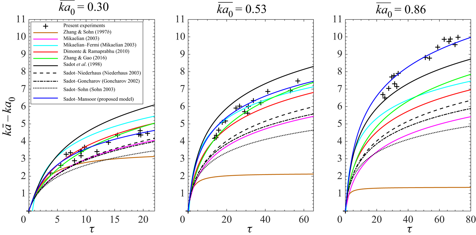
Figure 7. Evolution of dimensionless overall amplitude  $(k\bar {a}-ka_{0})$ versus dimensionless time $\tau$ found in present experiments in comparison with past nonlinear models based on heuristic/interpolation methods (Sadot et al. Reference Sadot, Erez, Alon, Oron, Levin, Erez, Ben-Dor and Shvarts1998; Mikaelian Reference Mikaelian2003), Padé approximation approach (Zhang & Sohn Reference Zhang and Sohn1997b) and simulations (Dimonte & Ramaprabhu Reference Dimonte and Ramaprabhu2010). Asymptotic components are $E_{b/s} = \frac{3}{2}\frac{(1 \pm\, A)}{(1 + A)} $ (solid black line); $E_{b/s} = 1 \pm A$ (black dashed line); $E_{b/s} = 3 \frac{(1 \pm\, A)}{3 \pm\, A}$ (black dash-dotted line); $E_{b/s} = \frac{(2 \pm\, A)}{2}$ (black dotted line); and $E_{b/s} = \ln \big(\frac{3}{ka_0}\big)\frac{(1 \pm\, A)}{(1 + A)}$ (blue solid line).
Table 2. Summary of nonlinear models for single-mode perturbations showing their equation, pre-shock scaled initial amplitudes and non-dimensional time range considered.
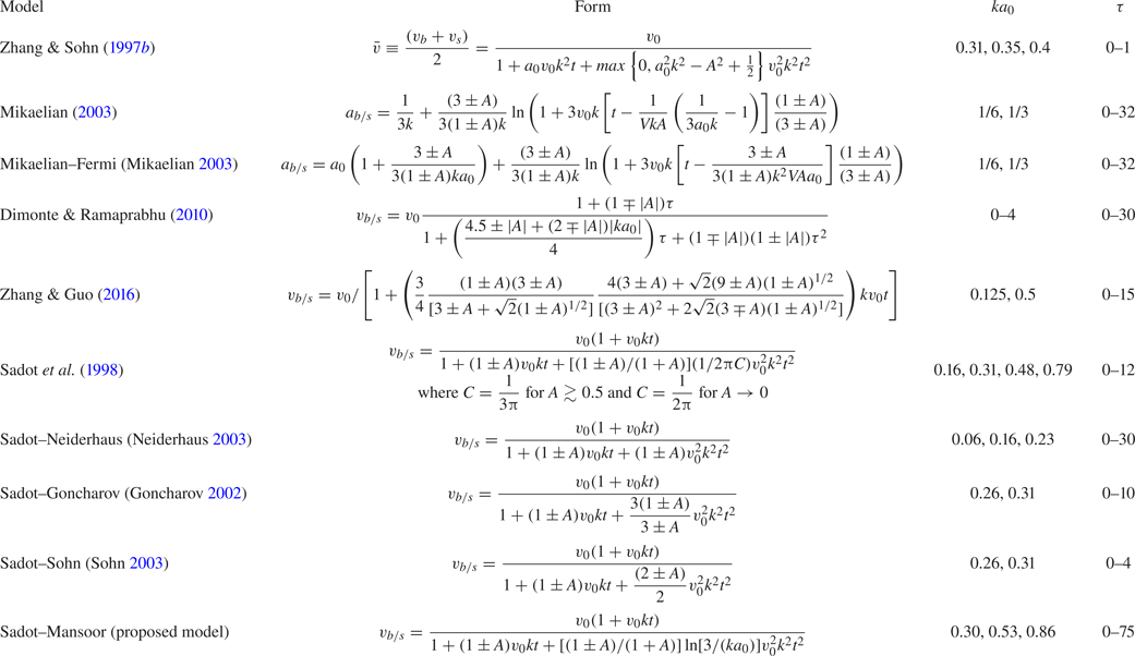
Sadot et al.'s model and its asymptotic  $E_{b/s}$ variants from previous studies in addition to Zhang & Gao have repeating evolution profiles from not having an explicit dependence on $ka_0$. Dimonte & Ramaprabhu's correction for this dependence was based on numerical simulations validated with experiments (Niederhaus & Jacobs Reference Niederhaus and Jacobs2003; Jacobs & Krivets Reference Jacobs and Krivets2005) and models (Zhang & Sohn Reference Zhang and Sohn1997b; Sadot et al. Reference Sadot, Erez, Alon, Oron, Levin, Erez, Ben-Dor and Shvarts1998; Mikaelian Reference Mikaelian2003) for $A \sim 0.2\text {--}0.7$, $ka_0 = 0.26\text {--}0.375$ at early–intermediate times ( $\tau = 0\text {--}30$). The model proposed showed noticeable deviation from experimental results for $A \sim 1$, $ka_0 > 1$ at $\tau = 1$. The long-duration experiments conducted here in comparison explore an extended late-time regime up till $\tau \approx 75$ for large $ka_0$ initial conditions which these 2-D single-mode nonlinear models are not intended for. This could explain the deviation from modelling predictions for $\overline {ka_0} =0.86$ noted in figure 7. An extreme example of this discrepancy appears in Zhang & Sohn's model where no growth is noted after a time $\tau$, manifesting itself earlier for higher $ka_0$. Alternatively, the RMI evolution herein may be affected by multi-modal features observed at the interface, especially at the asymptotic stage, leading to deviations from single-mode theory at late times. It is noteworthy that the small-scale instabilities may have a three-dimensional nature that can alter overall growth and contribute to the discrepancy observed as well.
Accounting for an explicit dependence on  $ka_0$ that captures our experimental results, we propose a variant of Sadot et al.'s empirical rational function
 \begin{equation} E_{b/s} = \frac{(1 \pm A)}{(1+A)}\ln\left( \frac{3}{ka_0} \right) \end{equation}
to characterize the asymptotic behaviour of the perturbation growth. This modification provides a much better agreement with our late-time amplitude measurements for increasing  $ka_0$ values. Similar to Dimonte & Ramaprabhu and Zhang & Zhao, the model predicts an intermediary growth between Mikaelian (Reference Mikaelian2003) and Sadot et al. (Reference Sadot, Erez, Alon, Oron, Levin, Erez, Ben-Dor and Shvarts1998) for $\overline {ka_0} = 0.30$ $(A^- = 0.67)$. The growth rates increase with the scaled initial amplitudes in order to match the experimental measurements. More importantly, the $1/t$ asymptotic dependence expected from potential flow theory plays an important role in obtaining good agreement with our extended late-time measurements which has also been observed in the experiments of Collins & Jacobs (Reference Collins and Jacobs2002) and Niederhaus & Jacobs (Reference Niederhaus and Jacobs2003).
It is important, however, to mention that this asymptotic variant of Sadot et al.'s model proposed is based on the evolution of dominant modes where multi-modal features and residual small perturbations are also present. Therefore caution must be taken in its applicability to predict the evolution of purely single-mode RMI experiments. The present experiments instead are designed to understand how multi-modal features evolve given a dominant single mode to reflect real-world RMI conditions more accurately. Since modelling such a complex flow is difficult, the need to understand how it develops empirically (as represented by 3.6 and 3.15) is very important. The membraneless method developed herein to set up initial conditions does not suffer from additional disturbances in the form of small-scale perturbations caused by membrane rupture following shock passage. The use of a dominant mode with other residual small perturbations as an inevitable artifact of machine-made interfaces are complementary to single-mode work in the RMI community and will be extremely beneficial in developing RMI growth models closer to reality.
3.3. Vortex identification and invariants of the reduced velocity gradient tensor
Vortical structures resulting from the baroclinic generation of vorticity in RMI flows can significantly enhance mixing (Peng et al. Reference Peng, Zabusky and Zhang2003). While mixing at the smallest scales affects molecular level processes directly, with energy converted into heat by viscous dissipation, large-scale mixing in the range of integral length scales drawing energy directly from the mean flow can have an indirect influence by advecting fluid through regions where turbulence characteristics are substantially variant (Ducci & Yianneskis Reference Ducci and Yianneskis2007). Vortical motions can aid macro-mixing processes and mixing transition significantly, yet little is known in terms of their size–strength characteristics and initial condition dependence in RMI flows.
The identification of vortex structures in 3-D velocity field data can be performed using various velocity gradient tensor (VGT) based mathematical schemes. Among the methods proposed include the  $Q$-criterion (Hunt, Wray & Moin Reference Hunt, Wray and Moin1988), $\varDelta$-criterion (Chong, Perry & Cantwell Reference Chong, Perry and Cantwell1990), $\lambda _{ci}$-criterion (Zhou et al. Reference Zhou, Adrian, Balachandar and Kendall1999) and $\lambda _2$-criterion (Jeong & Hussain Reference Jeong and Hussain1995). The $Q$-criterion defines a vortex as a connected fluid region where the second invariant of the velocity gradient tensor ( $\boldsymbol {\nabla } u$) is positive, $Q > 0$. Decomposing the tensor into symmetric and anti-symmetric parts, the second invariant of the full VGT for an incompressible flow (applicable following the traversal of a low Mach number shock through the interface) can be expressed as
 \begin{equation} Q = \tfrac{1}{2} \left(||\varOmega||^2 - ||S||^2 \right), \end{equation}
where
 \begin{equation} S_{ij} = \frac{1}{2} \left(\boldsymbol{\nabla} u + (\boldsymbol{\nabla} u)^{\textrm{T}} \right) = \frac{1}{2} \left(\frac{\partial u_i}{\partial x_j} + \frac{\partial u_j}{\partial x_i} \right) \end{equation}
is the strain-rate tensor and
 \begin{equation} \varOmega_{ij} = \frac{1}{2} \left(\boldsymbol{\nabla} u - (\boldsymbol{\nabla} u)^{\textrm{T}} \right) = \frac{1}{2} \left(\frac{\partial u_j}{\partial x_i} - \frac{\partial u_i}{\partial x_j} \right) \end{equation}
is the rotation-rate tensor. The  $Q$-criterion represents a local balance between rotation and strain, identifying vortices as regions where the magnitude of vorticity is larger than that of strain rate.
Obtaining planar PIV measurements, such as in this study, omits the out-of-plane velocity components, truncating the full VGT that can be used for vortex identification analysis. The  $2 \times 2$ reduced VGT formed from a 2-D slice of the 3-D flow field is given by
 \begin{equation} \boldsymbol{\nabla} \tilde u = \begin{bmatrix} \dfrac{\partial u}{\partial x} & \dfrac{\partial u}{\partial y} \\ \dfrac{\partial v}{\partial x} & \dfrac{\partial v}{\partial y} \end{bmatrix} \end{equation}
which represents the upper-left  $2 \times 2$ portion of the full VGT ( $\boldsymbol {\nabla } u$) containing streamwise and spanwise velocity gradients. The characteristic polynomial of $\boldsymbol {\nabla } \tilde u$ is
 \begin{equation} \lambda^2 + p\lambda + q = 0, \end{equation}
where  $p$ and $q$ represent the first and second invariants of (3.20), respectively, given by
 \begin{gather} p = -\mathrm{tr}(\boldsymbol{\nabla} \tilde u) = - \frac{\partial u}{\partial x} - \frac{\partial v}{\partial y}, \end{gather}
 \begin{gather}q = \mathrm{det}(\boldsymbol{\nabla} \tilde u) = \frac{\partial u}{\partial x} \frac{\partial v}{\partial y} - \frac{\partial u}{\partial y} \frac{\partial v}{\partial x}. \end{gather}
This expression for  $q$ is not an assessment of local rotation excess over strain rate, producing positive values for irrotational flows in sources and sinks. A more robust criterion can be obtained by simplifying (3.16) in terms of the reduced VGT giving (Chen et al. Reference Chen, Zhong, Qi and Wang2015)
 \begin{equation} Q = - \frac{\partial u}{\partial y} \frac{\partial v}{\partial x} - \frac{1}{2}\left[\left(\frac{\partial u}{\partial x}\right)^2 + \left(\frac{\partial v}{\partial y} \right)^2\right] \equiv \frac{\partial u}{\partial x} \frac{\partial v}{\partial y} - \frac{\partial u}{\partial y} \frac{\partial v}{\partial x} - \frac{1}{2} \left( \frac{\partial u}{\partial x} + \frac{\partial v}{\partial y} \right)^2, \end{equation}
where connected fluid regions with  $Q > 0$ are identified as vortices in planar velocity fields.
The strength of the vortical motion can be quantified using the  $\lambda _{ci}$-criterion where $\lambda _{ci}$ corresponds to the imaginary part of the complex eigenvalues of the VGT. This method follows from the $\varDelta$-criterion which associates swirling regions with complex eigenvalues of the VGT and examines the discriminant of the characteristic polynomial as a potential vortex indicator. As such, connected regions having a positive discriminant from the full VGT and negative discriminant from the reduced VGT are equivalent to having complex conjugate eigenvalues for vortex identification. While the $\lambda _{ci}$ and $\varDelta$-criteria are based on same definition, the former has the added advantage of being a measure of the local swirling strength of the vortex also referred to as the swirl-strength criterion (Zhou et al. Reference Zhou, Adrian, Balachandar and Kendall1999).
We use the  $Q$-criterion in conjunction with the $\lambda _{ci}$-criterion to extract vortices and their associated swirl strengths for increasing $\overline {ka_0}$ initial conditions. Figure 8 shows an example for criteria comparison where (a) a sample planar PIV image of the mixing width (from figure 2c) is presented with its (b) vorticity field and velocity fluctuation vectors and corresponding vortices identified by (c) $Q$ and (d) $\lambda _{ci}$ criteria. As expected, vorticity is mainly concentrated at the interface, acting to stretch its length and drive mixing. The two dimensional swirling motions observed in (c,d) represent cross-sections of 3-D structures which tend to have an elongated tubular form known as ‘vortex tubes’. The appearance of these structures projected onto a 2-D plane depends entirely on how they are angled with respect to that plane. A plane perpendicular to the axis of the vortex tube produces a circular projection while a sufficient angular deviation can render it as an ellipsoid or an elongated feature which is found to be a characteristic of most vortex structures identified in (c,d). Nevertheless, comparing the structures in (c,d), vortex regions common to both $Q$ and $\lambda _{ci}$ criteria are very similar with a slightly lesser number of vortices identified for the former method. This results from $Q$ imposing a more restrictive condition for vortex identification making it a subset of the $\lambda _{ci}$-criterion (Chen et al. Reference Chen, Zhong, Qi and Wang2015). Since the threshold for $\lambda _{ci}$ is not well-defined, we use $Q > 0$ to identify vortex regions and obtain the associated mean swirl strengths as corresponding values of $\overline {\lambda _{ci}}$.

Figure 8. (a) PIV image of the mixing width from example shown in figure 2 (c,  $t = 2.65$ ms) and corresponding plots for (b) vorticity, $\omega _z$, overlaid with velocity fluctuation vectors, (c) Q-criterion and (d) swirl strength, $\lambda _{ci}$.
Figure 9 shows the probability distribution of vortex sizes and mean swirl strengths obtained from eight instantaneous PIV realizations at  $t= 2.65$ ms (a,c) and 5.65 ms (b,d). Vortex sizes with mean diameters ranging between the Taylor micro-scales and integral length scales (see § 3.5) are considered to probe the macro-mixing characteristics of the flow with consistency between data sets. The total count ( $n$) increases with $\overline {ka_0}$ and time as the corresponding mixing widths are larger and contain more vortices from breakdown. The distribution of vortex sizes, however, remains unchanged for the different initial conditions as similar probabilities are noted across the spatial scale. Mean swirl-strength profiles in comparison also tend towards self-similar distributions eventually but have larger variations at the earlier time ( $t=2.65$ ms). These distributions show a peaking phenomenon for $\overline {\lambda _{ci}} \approx 0.5\text {--}1\times 10^3$ and a noticeable decrease for $\overline {\lambda _{ci}} \gtrsim 2\times 10^3$ between (c,d), indicating a larger presence of weaker vortices at late times.

Figure 9. Probability distribution of vortex size and swirl strength at  $t = 2.65$ ms (a,c) and 5.65 ms (b,d) for increasing $ka_0$ initial conditions. Counts are normalized with respect to total count $(n)$.
The distribution of vortex size with respect to mean swirl strength and its evolution can be examined by plotting the joint probability distribution of the two variables as shown in figure 10. The equiprobability contours generally increase in the abscissa (size) and decrease in the ordinate (strength) with time indicating a shift in probability towards larger weaker structures (a–d,b–e,c–f). The shift becomes increasingly noticeable for higher  $\overline {ka_{0}}$ interfaces where the expansion in macro-scale vortex structures is consistent with the corresponding increase in mixing layer thicknesses. The decrease in mean swirl strengths with time provides evidence of energy transfer from these vortex structures to smaller scales. Since larger viscous losses are associated with turbulence, the shift is expected to be more prominent for higher $\overline {ka_{0}}$ initial conditions from having earlier mixing transition onsets (see § 3.6).

Figure 10. Joint probability distribution of vortex size with swirl strength for  $\overline {ka_0}= 0.30$, 0.53 and 0.86 at $t= 2.65$ ms (a–c) and $t= 5.65$ ms (d–f), respectively.
The statistical properties of small-scale turbulence can be investigated following Cardesa et al.'s (Reference Cardesa, Mistry, Gan and Dawson2013) seminal work interpreting joint probability density functions (p.d.f.s) of invariants of the reduced VGT based on averages of  $p$ and $q$ under the assumption of local isotropy. Resorting to an average-based approach stems from the difficulty in capturing the local topology of 3-D structures based on their 2-D projection, as discussed previously. Their work showed that the joint p.d.f. of $p$–
$p$– $q$ has an asymmetric distribution resembling a teapot shape common to all fully developed turbulent flows. Since this asymmetry stems from a higher probability of quadrants in the $p$–
$p$– $q$ diagram where $p$ and $q$ are oppositely signed in comparison to quadrants where they carry same signs, it requires $\langle pq \rangle <0$. In addition, given $\langle pq \rangle = -\frac {1}{15} \langle w_i S_{ij} w_j \rangle$ assuming local isotropy, the inequality $\langle pq \rangle <0$ follows from the average enstrophy amplification $\langle w_i S_{ij} w_j \rangle >0$ indicating that the asymmetry in joint p.d.f.s of $p$–
$p$– $q$ results from the universal predominance of vortex stretching at the smallest scales.
The case of RMI flows in mixing transition herein gives the opportunity to investigate the evolution of these asymmetricities in joint p.d.f.s of  $p$–
$p$– $q$ and hence the predominance of small-scale vortex stretching in transitionally turbulent flows. Figure 11 shows normalized joint p.d.f.s of $p$–
$p$– $q$ for $\overline {ka_0}=$ 0.30, 0.53 and 0.86 at 2.65 ms (a,c,e) and 5.65 ms (b,d,f), respectively. As observed, plots (a,b) for the lowest $\overline {ka_0}$ representing flows before mixing transition (see § 3.6) show relatively flat apexes with nearly equal tail extensions along $q = p^2/4$. The parabola $q = p^2/4$ marks the boundary between real and imaginary roots of the characteristic polynomial of $\boldsymbol {\nabla } \tilde u$ and has a distinct influence on the p.d.f. shapes. Plots (c,d) and (e,f) in comparison for flows in the early and late stages of mixing transition, respectively (see § 3.6), exhibit an increasing resemblance with a teapot-like shape in time as a hump at the apex, spout-like extension along $q = p^2/4$ in the second quadrant and spread in the fourth quadrant become notable. $\langle pq \rangle / \langle \omega _3^2 \rangle ^{3/2}$ values computed for flows herein (see figure 11 caption) corroborate Cardesa et al.'s prediction that such asymmetric joint p.d.f. distributions of $p$–
$p$– $q$ are associated with $\langle pq \rangle <0$. In addition, since the flow is isotropic at the smallest scales (see § 3.6), negative $\langle pq \rangle$ quantities indicate the predominance of enstrophy amplification from vortex stretching at the smallest scales. Given RMI flows are time dependent, having a tendency towards turbulence with mixing in the nonlinear regime, the increasing teapot-like resemblance of the joint p.d.f.s with time indicates the potential in using $p$–
$p$– $q$ plots as a robust tool in determining mixing transition in 2-D diagnostics.

Figure 11. Normalized joint p.d.f.s of reduced VGT invariants  $p$ and $q$ for $ka_0= 0.30, 0.53$ and 0.86 at 2.65 ms (a,c,e) and 5.65 ms (b,d,f), respectively. Contour levels scale logarithmically. $\langle pq \rangle / \langle \omega _3^2 \rangle ^{3/2} = (a)\ -0.053$, (b) $-$0.029, (c) $-$0.062, (d) $-$0.029, (e) $-$0.065, (f) $-$0.054. $\omega _3 = (\partial u_2 / \partial x_1) - (\partial u_1/\partial x_2)$.
3.4. Turbulent statistics: velocity fluctuations and turbulent kinetic energy
Fluctuations in the velocity field generated by eddies driving mixing transition can give more information about the complex interactions of vortex structures. Because the motions associated with turbulent eddies are approximately random, the velocity fluctuations can be obtained using statistical methods. We use spanwise averaging (Balakumar et al. Reference Balakumar, Orlicz, Ristorcelli, Balasubramanian, Prestridge and Tomkins2012) for computing fluctuations from single realizations which for the ith velocity component are defined as
 \begin{gather} \overline{u_i}(x) = \overline{u_i(x,y)}^y, \end{gather}
 \begin{gather}u'_i(x,y) = u_i(x,y) - \overline{u_i}(x), \end{gather}
where superscripts  $x$ and $y$ denote averages in the streamwise and spanwise directions, respectively.
Figure 12 presents p.d.f.s of streamwise (a,b) and spanwise (c,d) velocity fluctuations for different initial conditions and times. The p.d.f.s are generated using velocity fields from eight instantaneous PIV realizations. Non-Gaussian profiles with a larger spread are generally noted for  $u'$ and $v'$ at $t = 2.65$ ms (a,c) in comparison to their corresponding p.d.f.s at $t = 5.65$ ms (b,d), respectively. While $u'$ profiles at the earlier time have a slight to moderate negative skewness (longer left tails), a positive skewness is noted at $t = 5.65$ ms downstream. This is noticeable as an inward shift of the left-side tails, i.e. in negative (downward) fluctuations indicating a decrease in the probability of large streamwise fluctuations in the shock-wave direction downstream. The p.d.f.s of spanwise $v'$ fluctuations tend to be narrower than the corresponding streamwise $u'$ profiles. Although the prior have similar distributions at $t = 5.65$ ms, the latter show an increasing spread with $\overline {ka_{0}}$ which reflects the presence of larger fluctuations. Because turbulence is characterized by large intermittent velocity fluctuations, with p.d.f.s in developing flows having long tails (Jiménez Reference Jiménez2000; Orlicz et al. Reference Orlicz, Balasubramanian, Vorobieff and Prestridge2015), this may indicate a higher level of intermittency for larger $\overline {ka_{0}}$ values. The differences between $u'$ and $v'$ p.d.f. profiles observed at both times also indicates the presence of anisotropy in the flow field.

Figure 12. Probability density functions of (a,b) streamwise,  $u'$ and (c,d) spanwise velocity fluctuations $v'$ at $t = 2.65$ ms (a,c) and $t= 5.65$ ms (b,d) for $\overline {ka_{0}}= 0.30, 0.53$ and 0.86. S represents skewness.
Velocity fluctuations from (3.25) can be used to obtain the spanwise-averaged 2-D turbulent kinetic energy  $K(x)$ across the fluid layer as
 \begin{equation} K(x) = \left[\tfrac{1}{2} \left( \overline{u'^2(x,y)}^y + \overline{v'^2(x,y)}^y \right)\right]^n, \end{equation}
where the superscript  $n$ represents the ensemble mean. Turbulent kinetic energy (TKE) estimates from (3.26) versus the normalized streamwise distance $\zeta = x/h$ are shown in figure 13. TKE values for $\zeta \gtrsim 0.6$ become closer for all three initial conditions with the passage of time. The differences appear in the upper half of the mixing region where larger $\overline {ka_{0}}$ initial conditions generally result in higher levels of turbulence; $K$ peaks between $0.5 \gtrsim \zeta \gtrsim 0.7$ at $t= 2.65$ ms and $0.3 \gtrsim \zeta \gtrsim 0.6$ at $t= 5.65$ ms with a decrease in magnitude over time due to viscous dissipation. The upward shift in peaks suggests strong velocity variances to drive mixing towards the less dense fluid (air) with time. This coincides with the characteristics of roll-up mechanisms in expanding and elongating spike mushroom structures (Peng et al. Reference Peng, Zabusky and Zhang2003) where fluid entrainment causes local mixing enhancements. Since the TKE peaks observed are much larger for the highest $\overline {ka_{0}}$ investigated, the mechanisms that drive mixing towards the less dense fluid seem increasingly effective for large initial amplitudes.

Figure 13. Two-dimensional TKE from (3.26) versus the normalized streamwise distance  $\zeta = x/h$ for $\overline {ka_{0}} =0.30,0.53$ and 0.86 at (a) $t= 2.65$ ms and (b) $t= 5.65$ ms.
3.5. Minimum state analysis and turbulent length scales
In this section, we further probe the state of the flow by characterizing turbulence using global and local measures of the Reynolds number and estimate the relevant turbulent length scales to determine the existence of an inertial range. Determining the transition to turbulence in time-dependent Richtmyer–Meshkov flows is crucial in understanding when viscous dissipation losses become significant in ICF applications. An important aspect of this problem is the effect of initial conditions on the turbulent transition with particular emphasis on the transition criterion used.
Since the unsteady nature of RMI flows involves continuously developing length and velocity scales, the definition of Reynolds number used to characterize turbulence must be chosen appropriately to determine flow transition with time. Several methods for the calculation of Reynolds number have been proposed in the literature yet the applicability and relative disparity in characterizing mixing transition of these methods remain questionable. Three different Reynolds number calculations based on local and global estimates are therefore considered for comparison purposes and investigating their physical significance in RMI flows.
A local Reynolds number based on turbulent fluctuations can be defined as  $Re_{\varDelta } = \delta ' h/\nu$ (Tomkins et al. Reference Tomkins, Balakumar, Orlicz, Prestridge and Ristorcelli2013). The velocity scale $\delta '$ is estimated from the width of $u'$ and $v'$ velocity fluctuation p.d.f.s (see e.g. figure 12) taken as the range 99 % of all fluctuations fall within. The average width of the velocity fluctuation p.d.f.s is used giving $\delta '= (\delta '_u + \delta '_v)/2$ and the characteristic outer length scale is taken as the width of the mixing layer $h$. The kinematic viscosity of the gaseous mixture can be estimated from Youngs (Reference Youngs1984) expression $\nu = (\mu _1 + \mu _2)/ (\rho _1 + \rho _2)$ where subscripts 1 and 2 represent the light and heavy gases, respectively. Using one-dimensional gas dynamics and normal shock relations, this produced a value of $\nu = 7.98 \times 10^{-6}\ \textrm {m}^2\ \textrm {s}^{-1}$.
The local information based estimate can be compared with global Reynolds number estimates based on circulation and mixing width growth rate measurements. The circulation Reynolds number is given by  $Re_{\varGamma } = \varGamma /\nu$ where $\varGamma$ represents the circulation of a vortex core or region. Considering positive and negative circulations in the flow field separately we obtain $Re_{\varGamma }^{+}$ and $Re_{\varGamma }^{-}$. These circulations are computed as the sum of local circulations from individual points in the velocity field where each local circulation occurs about the centre of a small region d $A$ sizing $2 \times 2$ vectors (Orlicz et al. Reference Orlicz, Balasubramanian and Prestridge2013). This can be expressed as
 \begin{equation} \varGamma(t) = \int\int_{A} \omega \,\mathrm{d}A . \end{equation}
A large-scale Reynolds number in RMI flows can also be defined as  $Re_{h} = h \dot {h}/\nu$ where $\dot {h}$ is the mixing width growth rate. Previous studies have not found $Re_{h}$ useful in understanding mixing physics or capturing transition in RM flows. Scattered values reported by Orlicz et al. (Reference Orlicz, Balasubramanian, Vorobieff and Prestridge2015) were attributed to mixing width growth rate measurements being affected by small perturbations at each time. Weber et al. (Reference Weber, Haehn, Oakley, Rothamer and Bonazza2014) overcame the spread by evaluating $Re_h$ using curve fits to the mixing width growth data which showed the results as lacking time dependence. This is expected since mixing growth rates decrease rapidly with time as mixing widths increase causing the velocity and length scale estimations in $Re_{h}$ to counteract each other. In our consideration of $Re_{h}$, $\dot {h}$ is taken as the initial perturbation growth rate from (3.12) giving $\dot {h} = 12.5\ \textrm {ms}^{-1}$, $21.2\ \textrm {ms}^{-1}$ and $31.9\ \textrm {ms}^{-1}$ for $\overline {ka_0}= 0.30, 0.53$ and 0.86, respectively.
It is desirable for the mixing transition criterion in RMI flows to be temporally flow dependent since the unsteady conditions result in continuously evolving length scales and the associated inertial range to develop accordingly. Dimotakis (Reference Dimotakis2000) proposed a minimum Reynolds number of  $1\text {--}2\times 10^4$ to achieve mixing transition in stationary flows which has been extended to a wide range of time-dependent flow studies (Robey et al. Reference Robey, Zhou, Buckingham, Keiter, Remington and Drake2003; Zhou et al. Reference Zhou, Remington, Robey, Cook, Glendinning, Dimits, Buckingham, Zimmerman, Burke and Peyser2003a; Zhou, Robey & Buckingham Reference Zhou, Robey and Buckingham2003b). While the stationary flow Reynolds number criterion is indeed a necessary condition, it is not a sufficient measure for achieving the minimum state in unsteady flows (Zhou Reference Zhou2007). The minimum state is described as the lowest laboratory–astrophysical representative Reynolds number a time-dependent flow must achieve such that the inertial range has extended sufficiently ( $\lambda _L/\lambda _v = 2$) to ensure the energy-containing scales are not contaminated by the dissipation scales. Here $\lambda _v = 50h \,Re^{-3/4}$ and $\lambda _L = 5h \,Re^{-1/2}$ denote the inner viscous scale and Liepmann–Taylor scale as the lower and upper limit of the inertial range, respectively (Dimotakis Reference Dimotakis2000). The temporal criterion for unsteady flow minimum state is thus reached when the Leipmann Taylor scale grows to become twice as large as the inner viscous length scale which provides $Re = 1.6 \times 10^{5}$ (Zhou Reference Zhou2007) as the critical Reynolds number to faithfully represent the spectral range measured in a laboratory setting to the corresponding astrophysical phenomenon.
The initial condition and time dependence of  $Re_{\varDelta }$, $Re_{\varGamma }$, $Re_{h}$ are plotted in figure 14. The Reynolds numbers increase with $\overline {ka_{0}}$ and $t$ where estimates from the circulation based approach are higher than those obtained from other methods; $Re_{\varDelta }$ and $Re_{h}$ values, however, occur within a factor of 2 of each other as also noted by Tomkins et al. (Reference Tomkins, Balakumar, Orlicz, Prestridge and Ristorcelli2013). While $Re_{\varGamma }$ generally exceeds the minimum state criterion (dashed lines), $Re_{\varDelta }$ values stay under and $Re_{h}$ values show a cross-over between $\overline {ka_{0}} = 0.53$ and 0.86 at both times. Assuming linear interpolation, the crossover occurs at lower $\overline {ka_{0}}$ values with increase in time indicating mixing transition to occur earlier for higher $\overline {ka_{0}}$ initial conditions. Given these trends are physically corroborated by the formation of mixing regions (see figure 2), $Re_{h}$ better characterizes the flow in terms of mixing transition compared to other methods used herein and demonstrates the physical significance of the minimum state criterion in the context of RMI studies.

Figure 14. Local and global information based Reynolds numbers,  $Re_{\varDelta } = f(u', h, \nu )$, $Re_{\varGamma }= f(\varGamma , \nu )$ and $Re_{h} = f(\dot {h}, h, \nu )$, versus $\overline {ka_{0}}$ at (a) $t= 2.65$ ms and (b) $t= 5.65$ ms. The dashed lines indicate the minimum state criterion of $Re= 1.6 \times 10^{5}$ by Zhou (Reference Zhou2007).
The separation between Taylor microscales and the integral lengths scales can also provide insight into the extension of the inertial range. The Taylor micro-scale can be estimated by performing the autocorrelation of velocity fluctuations in the spanwise direction such that
 \begin{equation} R(r) = \frac{ \langle \eta'(y) \eta'(y+r) \rangle}{(\eta')^2}, \end{equation}
where  $\eta '$ can represent either streamwise or spanwise fluctuations. Since $R(r)$ has a maximum at the origin, ${\textrm {d}^2R(0)}/{\textrm {d} r^2}$ is strictly negative. The Taylor microscale can then be defined based on the curvature of the autocorrelation function at $r=0$ as
 \begin{equation} \lambda_T = \left[ -\frac{1}{2} \frac{\textrm{d}^2R(0)}{\textrm{d} r^2} \right]^{-1/2}, \end{equation}
where  $\lambda _{T,u}$ is the transverse and $\lambda _{T,v}$ is the longitudinal Taylor microscale. The curvature is obtained by fitting a parabola to three points on each side of the autocorrelation origin, i.e. the seven central points. The corresponding integral length scales are simply the area under the autocorrelation function given by $L = \int _0^\infty R(r)\,\textrm {d} r$.
Since  $\lambda _T$ can be related to velocity derivatives (Pope Reference Pope2000), the Taylor microscales can be computed alternatively from
 \begin{equation} \lambda_{T,\eta} = \sqrt{\frac{2\overline{\eta'^2_i}}{\overline{(\textrm{d}\eta'_i/\textrm{d} x_i)^2}}}. \end{equation}
 Reynolds number scalings from local isotropy provide another Taylor microscale estimate following  $\lambda _{T} \approx ChRe^{-1/2}$ where the scaling factor $C$ can be taken as 2.3 (Weber et al. Reference Weber, Haehn, Oakley, Rothamer and Bonazza2014), $\sqrt {10}$ (Pope Reference Pope2000), $\sqrt {15}$ (Tennekes & Lumley Reference Tennekes and Lumley1972), 10 (Orlicz et al. Reference Orlicz, Balasubramanian, Vorobieff and Prestridge2015). Mohaghar et al. (Reference Mohaghar, Carter, Musci, Reilly, McFarland and Ranjan2017) showed Taylor microscales estimated using $C= \sqrt {15}$ to be 3–4 $\times$ smaller than measured results which was attributed to the presence of resolution effects. Weber et al. (Reference Weber, Haehn, Oakley, Rothamer and Bonazza2014) discussed that a similar discrepancy found using $C = 2.3$ could not be accounted by these effects in their set up indicating the need to modify traditional Reynolds number scaling laws for better agreement when applied to RMI flows. For this purpose, Orlicz et al. (Reference Orlicz, Balasubramanian, Vorobieff and Prestridge2015) proposed $C = 10$ as being a more suitable scaling factor for consistency with the velocity based Taylor microscale which has also been used herein.
As observed in figure 15, although Taylor microscales obtained from spatial gradients and auto correlation methods are in good agreement, they are still 3–4 $\times$ larger than scales derived from Reynolds numbers. The discrepancy here could result from the presence of resolution effects as comparisons with previous RMI experiments using a higher resolution with similar cross-flow conditions to form a diffuse layer interface (Orlicz et al. Reference Orlicz, Balasubramanian, Vorobieff and Prestridge2015) show the velocity based Taylor microscales to closely match our $Re$ based Taylor microscales ${\approx } 1$ mm. Evaluating these against the integral length scales, the highest $L/ \lambda _T$ ratios obtained are 4.6, 5.6, 7.0 for $\overline {ka_0}= 0.30, 0.53, 0.86$, respectively, at $t= 5.65$ ms. The increasing separation between micro and integral length scales suggests the presence of an inertial range to be more likely for higher $\overline {ka_0}$ initial conditions. A more detailed analysis is presented in the following section.

Figure 15. Comparison of Taylor micro-scales obtained using spatial gradient ( $\partial v/\partial y, \partial u/\partial y$) and autocorrelation ( $corr_{v}, corr_{u}$) methods with Reynolds number based derivatives ( $\lambda _{\varDelta }, \lambda _h, \lambda {\varGamma }^+, \lambda {\varGamma }^-$) from $\lambda _{T} \approx 10h Re^{-1/2}$ at (a) $t= 2.65$ ms and (b) $t= 5.65$ ms.
3.6. Energy spectrum analysis
We investigate the distribution of scales and the existence of an inertial range from the one-dimensional energy spectra of velocity field measurements. Previous RMI experiments have shown the presence of a  $k^{-5/3}$ inertial range (Vorobieff et al. Reference Vorobieff, Mohamed, Tomkins, Goodenough, Marr-Lyon and Benjamin2003; Reilly et al. Reference Reilly, McFarland, Mohaghar and Ranjan2015) with an exponential dissipation range in the scalar spectrum (Weber et al. Reference Weber, Haehn, Oakley, Rothamer and Bonazza2012). Zhou's (Reference Zhou2001) theoretical analysis suggested a $k^{-3/2}$ scaling to occur during a quasi-steady state (after the shock has traversed the interface with no other external effects acting on it) before forming the classical Kolmogorov $k^{-5/3}$ scaling at fully developed turbulence. Both scalings were also observed in the simulations of Thornber et al. (Reference Thornber, Drikakis, Youngs and Williams2010, Reference Thornber, Drikakis, Youngs and Williams2012) where a $k^{-3/2}$ range was driven by the RM instability and a $k^{-5/3}$ sub-inertial range occurred at high wavenumbers for late times. Simulations by Hill, Pantano & Pullin (Reference Hill, Pantano and Pullin2006), Grinstein, Gowardhan & Wachtor (Reference Grinstein, Gowardhan and Wachtor2011) and Lombardini, Pullin & Meiron (Reference Lombardini, Pullin and Meiron2012) found a $k^{-5/3}$ scaling, Tritschler et al. (Reference Tritschler, Olson, Lele, Hickel, Hu and Adams2014) a $k^{-3/2}$ scaling and Cohen et al. (Reference Cohen, Dannevik, Dimits, Eliason, Mirin, Zhou, Porter and Woodward2002) a $k^{-6/5}$ scaling within the inertial range. The disagreement in computational results stems from the sensitivity to initial (Zoldi Reference Zoldi2002) and inflow (Saugat et al. Reference Saugat, Garnier, Tromeur, Larcheveque and Labourasse2004) conditions and difficulties with characterizing subgrid-scale effects in large eddy simulations (Grinstein Reference Grinstein2009).
Although shock-induced mixing in RMI flows is characterized by inhomogeneous anisotropic unsteady turbulence, the state-of-the-art analysis still uses a theoretical framework with diagnostics designed for homogeneous isotropic phenomena. The one-dimensional energy spectra components are obtained from the fast Fourier transform (FFT) of velocity fluctuations in the horizontal direction with multiplication by its complex conjugate giving
 \begin{gather} E_{u'} = \mathrm{FFT}(u').\mathrm{conj}((\mathrm{FFT}(u')), \end{gather}
 \begin{gather}E_{v'} = \mathrm{FFT}(v').\mathrm{conj}((\mathrm{FFT}(v')), \end{gather}
where  $E_{u'}$ is the energy spectrum of the streamwise velocity component; $E_{v'}$ is the energy spectrum of the spanwise velocity component. As per the Nyquist frequency constraint, only the first half of each component is sampled. Both components are averaged vertically and summed to give the total kinetic energy spectrum at a given time as $E(k_y)$.
Figure 16 shows the one-dimensional energy spectra  $E(k_y)$ for the three initial conditions at (a) $t= 2.65$ ms and (b) $t=5.65$ ms. Higher energy levels are found to be associated with higher $\overline {ka_{0}}$ initial conditions at $t= 2.65$ ms. Increasing times in the compensated spectrum plots show energy decay at small wavenumbers, $k_y \leq 250$ for $\overline {ka_{0}} =0.30$ (c) and $k_y \leq 100$ for $\overline {ka_{0}} =0.53$ (d) with an increase at larger wavenumbers indicating a transfer of energy from large to small scales. Energy losses for $\overline {ka_{0}} =0.86$ (e) are noticeably large across all wavenumbers. This is expected in correspondence with the evolution of a more turbulent transition noted in figure 14 with higher viscous losses. For $\overline {ka_{0}}= 0.30$ (c), 0.53 (d) and 0.86 (e), the spectra follow the classical Kolmogorov $-5/3$ power law in the ranges $k_y \approx 400\text {--}1000$, 300–1500, 150–1500 at $t= 2.65$ ms and $k_y \approx 500\text {--}1500$, 150–1500, 200–2000 at $t= 5.65$ ms, respectively. This shows a full decade of inertial range existing at $t=5.65$ ms for $\overline {ka_{0}} = 0.53$ and at both times for $\overline {ka_{0}} = 0.86$, indicating transition to turbulence. These findings corroborate trends noted in figure 14 where higher $\overline {ka_{0}}$ initial conditions experience earlier mixing transitions.

Figure 16. Energy spectra for  $\overline {ka_{0}}= 0.30, 0.53$ and 0.86 at (a) $t= 2.65$ ms and (b) $t= 5.65$ ms. Compensated spectra for $\overline {ka_{0}}= 0.30$ (c), 0.53 (d) and 0.86 (e) at both times.
Testing the degree of local isotropy, we plot the normalized cross-correlation spectrum between  $u'$ and $v'$ defined as $|E_{u'v'}(k_y)|/[E_{u'u'}(k_y)E_{v'v'}(k_y)]^{1/2}$ (Tavoularis & Corrsin Reference Tavoularis and Corrsin1981; Mohaghar et al. Reference Mohaghar, Carter, Musci, Reilly, McFarland and Ranjan2017) in figure 17. While the flow is generally anisotropic at large scales, a significant range of smaller scales ( $k_y \geq 700$) exhibit local isotropy at both times, $t= (a)$ 2.65 ms, (b) 5.65 ms. The smallest $\overline {ka_{0}}$ initial condition investigated corresponds to the least tendency towards isotropy at these scales. Trends in local isotropy remain mainly unaltered in time indicating the flow to retain its memory downstream for smaller scales. Anisotropy noted at the largest scales for $\overline {ka_{0}}= 0.30$ and 0.53 ( $t= 2.65$ ms) shifts towards the mid-range scales downstream ( $t= 5.65$ ms). The decrease in spectrum for $\overline {ka_{0}}= 0.86$ meanwhile indicates a breakdown from large to small scales. Decreasing levels of anisotropy for higher $\overline {ka_{0}}$ are noted for $k_y < 700$ at $t= 5.65$ ms. This reasonably stems from the earlier mixing transition of higher $\overline {ka_{0}}$ initial conditions resulting in finer turbulent scales.

Figure 17. Normalized cross-correlation spectrum for  $\overline {ka_{0}}= 0.30, 0.53$ and 0.86 at (a) $t= 2.65$ ms and (b) $t= 5.65$ ms.
4. Summary and conclusions
This study investigates the effect of initial conditions on the late-time growth and mixing transition of Richtmyer–Meshkov instability from sinuous perturbations on an air/sulphur hexafluoride interface ( $A \sim 0.67$) subjected to a Mach 1.2 planar shock wave. The experiments are performed at the vertical shock tube facility at Los Alamos National Laboratory. Interface perturbations are established using a membraneless technique where cross-flowing air and SF $_6$ separated by an oscillating splitter plate enter the shock tube with an undulating structure. The initial condition instabilities are not perfectly sinusoidal and comprise of asymmetric multi-modal features with residual small perturbations. A dominant wavelength and amplitude, however, are still observed. This allows understanding how multi-modal features evolve given a dominant single mode to reflect real-world conditions more accurately. A combination of oscillating plate frequencies and sweeping angles are used to investigate the effect of three different initial conditions $\overline {ka_{0}}= 0.3$, 0.53 and 0.86 where $k$ denotes the wavenumber and $a_0$ represents the initial amplitude of the dominant mode. We find that:
(i) Previous modelling predictions generally show growths devoid of initial condition dependency producing notable discrepancies between present experimental results for large $ka_0$ initial conditions. Accounting for an explicit $ka_0$ dependence in Sadot et al.'s (Reference Sadot, Erez, Alon, Oron, Levin, Erez, Ben-Dor and Shvarts1998) model, a modified empirical rational function that captures the asymptotic behaviour of the perturbation growth for $0.30 \leq \overline {ka_0} \leq 0.86$ is given by
(4.1)\begin{equation} v_{b/s} = \frac{v_0(1+v_0 kt)}{1+ (1 \pm A)v_0 kt + [(1 \pm A)/(1+A)]\ln[3/(ka_0)] v_0^2 k^{2} t^{2}}. \end{equation}
$ka_0$ initial conditions. Accounting for an explicit $ka_0$ dependence in Sadot et al.'s (Reference Sadot, Erez, Alon, Oron, Levin, Erez, Ben-Dor and Shvarts1998) model, a modified empirical rational function that captures the asymptotic behaviour of the perturbation growth for $0.30 \leq \overline {ka_0} \leq 0.86$ is given by
(4.1)\begin{equation} v_{b/s} = \frac{v_0(1+v_0 kt)}{1+ (1 \pm A)v_0 kt + [(1 \pm A)/(1+A)]\ln[3/(ka_0)] v_0^2 k^{2} t^{2}}. \end{equation}(ii) Comparing the minimum state criterion (
$Re = 1.6 \times 10^{5}$) for unsteady flows by Zhou (Reference Zhou2007) with various local and global Reynolds number estimates, the onset of mixing transition is found to occur earlier for higher $\overline {ka_{0}}$ initial conditions. This temporal criterion describes the lowest turbulent flow Reynolds number where the inertial range has extended sufficiently ($\lambda _L/\lambda _v = 2$) such that the energy containing scales do not interact with the dissipation scales.(iii) Mixing transition prescribed by the minimum state criterion is physically corroborated by interface break-up and formation of mixing regions. In addition, the one-dimensional energy spectra of velocity field measurements show a full decade of the classical
$k^{-5/3}$ inertial scaling to exist in corresponding flow conditions. Both findings demonstrate the physical significance of the minimum state criterion in RMI flows.(iv) The Reynolds number criterion (
$Re = 1\text {--}2\times 10^{4}$) by Dimotakis (Reference Dimotakis2000) is indeed a necessary condition for achieving mixing transition in stationary flows but not a sufficient measure in the case of time-dependent Richtmyer–Meshkov instability flows.(v) RMI flows in turbulent transition show an increasing teapot-like resemblance for joint p.d.f.s of
$p$–$q$ (invariants of the reduced VGT) with time. The asymmetry noted is associated with negative values of $\langle pq \rangle$ which along with local isotropy at the smallest scales indicates the predominance of enstrophy amplification and hence vortex stretching.


The evolution of  $p$–
$p$– $q$ plots into a teapot profile with mixing transition indicates the potential in using the technique as a valid tool for turbulence detection and estimation in 2-D diagnostics. This is particularly useful in ICF applications where diagnostics are limited by spatial constraints and determining the transition to turbulence is crucial in understanding when viscous dissipation losses become significant.
Acknowledgements
The authors would like to thank C. Lai for discussions on the reduced VGT analysis and S. Mula for help with the LabVIEW code. This research was partially supported by the Laboratory Directed Research & Development (LDRD) program at Los Alamos National Laboratory.
Declaration of interests
The authors report no conflict of interest.


 Open access