


1. Introduction
Jets are free shear flows that originate from a localised source of momentum. Similar to buoyancy-driven plume flows, jets are turbulent in most cases of practical interest, exhibiting chaotic motion and having a high Reynolds number  $Re = UL/\nu$, where $U$ is a velocity scale of the jet, $L$ a characteristic length scale, e.g. the jet radius, and $\nu$ the kinematic viscosity of the fluid. Given their ubiquitous nature and practical importance in a variety of geophysical and industrial scenarios, numerous investigations on the dynamics of turbulent jets have been performed over the past 70 years. In one of the earliest, Albertson et al. (Reference Albertson, Dai, Jensen and Rouse1950) studied the development of a pure jet, that is, one driven by momentum only, discharged into a quiescent uniform ambient. Although of great theoretical interest, such an idealised scenario is rather uncommon. In many real-world cases, a jet contains one or more scalar components which contribute to its density, making the jet more or less dense than the surrounding fluid. Such flows are commonly termed ‘buoyant jets’, with one example being the discharge of thermal effluent from a steam-electric power plant. The effluent is often warmer and thus lighter than the water in the reservoir it is discharged into, resulting in a rising jet motion. The ability to predict the dynamics and ultimate fate of buoyant jet fluid is of crucial importance for numerous ecological, environmental and industrial reasons, and has motivated various authors to investigate the dynamics of buoyant jets theoretically (Hirst Reference Hirst1971; Chen & Rodi Reference Chen and Rodi1980; Jirka Reference Jirka2004) and experimentally (Lane-Serff, Linden & Hillel Reference Lane-Serff, Linden and Hillel1993; Roberts, Ferrier & Daviero Reference Roberts, Ferrier and Daviero1997; Bloomfield & Kerr Reference Bloomfield and Kerr2002). These investigations deal with jet flows containing only one scalar component, which contributes to its density. Herein, we will refer to such jets as ‘single diffusive’.
It is, however, not uncommon for a jet fluid to contain two (or more) scalar components which contribute to its density and diffuse at different rates, e.g. heat and salt. We refer to such jets as ‘double diffusive’, with one example being waste brine discharged from a desalination plant into the ocean. The brine is warmer and saltier that the ambient ocean water, and hence the resulting jet is double diffusive.
For a particular fluid–solute combination, the Prandtl number  $Pr=\nu / \kappa _T$ and the Lewis number $\tau =\kappa _T / \kappa _S$ are pre-determined, making the dynamics of double-diffusive processes dependent on the dimensionless parameter $R_{\rho } = (\beta _T \Delta T) / (\beta _S \Delta S)$, where $\kappa _T$, $\kappa _S$ and $\beta _T$, $\beta _S$ are, respectively, the molecular diffusivities and the expansion coefficients for the faster-diffusing component $T$ and the slower-diffusing component $S$, and $\varDelta$ refers to the difference in the quantity between the jet and the ambient. In the hot and salty (‘thermohaline’) case, $\kappa _T = 1.4\times 10^{-7}\ \textrm {m}^2\,\textrm {s}^{-1}$, $\kappa _S = 1.5 \times 10^{-9}\ \textrm {m}^{2}\,\textrm {s}^{-1}$ and the dimensionless parameter $R_{\rho }$, commonly referred to as the ‘density ratio’, is a measure of the relative contributions of temperature and salt to the total departure of fluid density $\rho$ from a reference value $\rho _{r}$. For a thermohaline discharge into a fresh and cold uniform ambient, $\rho _{r}$ can be taken as the density of the ambient $\rho _a$, with $\Delta T$ and $\Delta S$ being the respective temperature and salinity differences between the discharged fluid and the ambient. Typically, the density ratio for such double-diffusive flows is either $0 < R_{\rho } < 1$ or $R_{\rho } > 1$, corresponding to the discharged fluid being denser or lighter than the ambient, respectively. The values of $R_{\rho } = 0$ and $R_{\rho } = \infty$ correspond, respectively, to single-diffusive buoyant saline and thermal jets. For the particular case of $R_{\rho } = 1$, the jet fluid density matches that of the ambient, making it neutrally buoyant.
In general, depending on whether the faster- or slower-diffusing component is unstably distributed, double-diffusive processes can exist in two distinct regimes. In the case where the faster-diffusing component ( $T$) is unstably distributed, the system is in the so-called ‘diffusive’ regime. The opposite case of an unstable distribution of the slower-diffusing component ( $S$) results in the ‘salt-fingering’ regime, potentially leading to the development of salt-fingering instabilities. Double-diffusive processes in both configurations have received considerable attention in applications to oceanography, geology and metallurgy (Huppert & Turner Reference Huppert and Turner1981) and the reader is referred to Radko (Reference Radko2013) for an in-depth overview of the field.
Given their ubiquity, it is somewhat surprising that, unlike single-diffusive jets, the dynamics of double-diffusive turbulent jets has received comparatively little research attention. This could be the result of an extrapolation of a widespread assumption that for flows at high Reynolds and Péclet numbers, slow molecular diffusive processes have little effect on the overall dynamics of the flow (Hunt & Van den Bremer Reference Hunt and Van den Bremer2011). Although this assumption is valid for single-diffusive turbulent flows, demonstrated through previously noted agreement between heat-only and salt-only turbulent plumes at various scales (Briggs Reference Briggs1982), double diffusion can have a considerable effect on the dynamics of turbulent shear flows. This was demonstrated recently by Dadonau, Partridge & Linden (Reference Dadonau, Partridge and Linden2020), who found experimentally that double-diffusive processes can lead to a considerable reduction in the entrainment coefficient of turbulent plumes. In application to jets, the importance of double-diffusive processes was first demonstrated by Thangam & Chen (Reference Thangam and Chen1981) in their experimental investigation of two-dimensional surface discharges of heated and/or saline jets into a stable salinity gradient. They observed that for the case of heated saline buoyant discharges, temperature and salinity were able to spread significantly deeper as compared to an analogous heated jet, which was attributed to the action of salt-fingering convection. More recent observation of the presence of salt fingers in turbulent double-diffusive jets was made by Law, Ho & Monismith (Reference Law, Ho and Monismith2004). In this work they also reported that initially neutrally buoyant round jets sink and found qualitative features that inspired us to explore this topic more quantitatively. Other related studies include the experimental investigations of double-diffusive lock-exchange flows (Yoshida, Nagashima & Ma Reference Yoshida, Nagashima and Ma1987) and gravity currents (Maxworthy Reference Maxworthy1983). More recently, detailed numerical investigations of double-diffusive effects in gravity currents were performed by Konopliv & Meiburg (Reference Konopliv and Meiburg2016) and Penney & Stastna (Reference Penney and Stastna2016).
In this work, we investigate experimentally the effect of double diffusion on the dynamics of turbulent round jets discharged into a quiescent fresh ambient. For our experiments we chose to work with the aqueous system in which a hot and salty (thermohaline) jet is discharged into cooler fresh water. For this combination, the component with the larger molecular diffusivity  $\kappa _T$ is temperature $T$ and that with the smaller molecular diffusivity $\kappa _S$ is salinity $S$. The Lewis number $\tau = \kappa _T / \kappa _S$ is $O(100)$, and therefore even for moderate concentration gradients of both components, the system can be strongly doubly diffusive. To simplify our analysis, we restricted our attention to initially neutrally buoyant jets discharged horizontally, with the only control parameters being the source scalar concentrations ( $\Delta S_0, \Delta T_0$) and the source Reynolds number $Re_0=U_0r_0/\nu$, where $U_0$ and $r_0$ are the source horizontal velocity and outlet radius, respectively.
The rest of the paper is structured as follows. In § 2 we describe the experimental set-up and the procedure followed to create neutrally buoyant double-diffusive jets. We then summarise and discuss instantaneous and time-averaged visual observations in § 3, highlighting the key features of double-diffusive jets and propose explanations for the observed behaviour. Finally, in § 4 a series of conclusions are drawn.
2. Experimental procedure
All experiments were conducted in a large transparent tank, measuring  $2.5\ \textrm {m} \times 0.70\ \textrm {m} \times 0.80\ \textrm {m}$ ( $L \times W \times H$), filled with fresh water. Figure 1 shows a schematic diagram of the entire experimental set-up. Turbulent jets were created by steadily ejecting source solution through a nozzle into the ambient fluid using a gear pump, which was carefully calibrated over the range of volume fluxes used, $3.0<Q_0<7.0\ \textrm {ml}\,\textrm {s}^{-1}$. The typical error of the source flow rate did not exceed ${\pm }0.05\ \textrm {ml}\,\textrm {s}^{-1}$, which was estimated as two standard deviations about the mean flow rates measured during calibration. Given the moderate source Reynolds numbers ( $700<Re_0<1500$), the jet fluid had to be additionally excited to produce turbulent flow at the point of discharge. This was achieved by ejecting the fluid through a nozzle, specifically designed to promote turbulence within the flow. The nozzle, originally designed by Professor P. Cooper and illustrated schematically in Hunt & Linden (Reference Hunt and Linden2001), achieves this by passing the flow through a ‘pin-hole’ (diameter 1 mm) and then into a wide expansion chamber (diameter 10 mm), ultimately leading to the circular nozzle outlet of radius $r_0=1.5\ \textrm {mm}$. The sharp expansion acts to excite turbulent flow in the chamber prior to discharge from the nozzle.

Figure 1. A schematic representation of the experimental set-up.
Temperature measurements of the source fluid in all experiments were obtained from two T-type thermocouples inserted into the nozzle, as shown schematically in figure 2. The nozzle had two insulated channels leading to the expansion chamber, allowing direct access to the source fluid near the ejection point. Done in this way, the thermocouple tips were submerged fully into the fluid flow in the expansion chamber, minimising the noise signal from the ambient, and had precise and secure positioning. The slots were positioned with 10 mm horizontal spacing, with the distance upstream from the nozzle outlet to the nearest thermocouple fixed at 10 mm. The geometry of the nozzle did not allow closer positioning of the thermocouples to the source outlet. The temperature drop between the upstream and downstream thermocouples varied for different source volume fluxes and temperatures, but was always of order  $\sim\!0.1\,^{\circ}{\rm C}$. The temperature at the point of discharge was estimated for each experiment individually by linearly extrapolating the temperature loss over the 10 mm spacing between the thermocouples to the nozzle outlet. The temperature of the ambient fluid was measured using four additional T-type thermocouples, located near the nozzle at a regular vertical spacing of 150 mm inside the tank. All thermocouples were calibrated in DigiFlow by placing them in a water bath over an appropriate temperature range ( $15\text {--}70\,^{\circ }\textrm {C}$), with an accuracy of ${\pm }0.1\,^{\circ }\textrm {C}$. Measurements were taken at 5 Hz using National Instruments equipment (NI 9213).

Figure 2. A schematic representation of the nozzle with inserted thermocouples and the siphon collecting the ejected jet fluid (see text for dimensions). Note the siphon was only used during the purging stage of an experiment.
In order to create neutrally buoyant double-diffusive jets, the density of the source fluid at the point of discharge had to be carefully matched to that of the ambient. This was achieved with great care for every experiment individually, as even small fluctuations of the source/ambient water temperature would lead to immediate deviation from neutral buoyancy. These temperature fluctuations would normally arise as a result of varying ambient room conditions, or as an expected consequence of changing the injection volume flux, which altered the amount of time the source fluid would spend exchanging heat with the ambient on its way to the nozzle.
With these challenges in mind, we developed the following experimental procedure. The experimental tank was always filled with fresh water and left overnight to equilibrate with the ambient room temperature. Each time, prior to the actual experiment, we first performed a test experiment, aimed at determining the temperature of the jet fluid at the point of discharge for given ambient conditions. To that end, source fluid of some unknown low salinity (unimportant at this stage) was warmed up using the 1 kW Grant LTC4 water bath to some fixed temperature (e.g.  $50\,^{\circ }\textrm {C}$). Once a steady-state temperature was reached, fluid ejection into the tank and temperature measurements were simultaneously initiated. Throughout each test experiment, a siphon (diameter 10 mm) was used to collect the ejected source fluid, thus avoiding thermal and dye contamination of the tank prior to the actual experiment. The siphon was connected to an additional gear pump, running at double the ejection volume flux and positioned 5 mm away from the nozzle outlet, ensuring that all ejected fluid was collected. Visual inspection using a small amount of dye showed that the siphoning process did not introduce noticeable disturbances to the ambient fluid. Moreover, the siphoning had no significant effect on the temperature readings. For all experiments, we found that steady-state temperature was reached within 500 s. To determine the steady-state source temperature we averaged the values taken over 50 s in steady state. This was used as a prediction of source temperature $T_0$ for the actual experiment, which was performed in the same conditions shortly after.
For the actual experiment, we first measured the density of the ambient fluid. This was then used to calculate the required source fluid salinity  $S_0$ such that the jet would be neutrally buoyant, given the source fluid temperature $T_0$ measured in the test experiment as detailed above. The required salinity $S_0$ was evaluated using the third-order equations of state of Ruddick & Shirtcliffe (Reference Ruddick and Shirtcliffe1979). Densities were measured by an Anton Paar DMA5000 density meter with an accuracy of ${\pm }10^{-6}\ \textrm {kg}\,\textrm {m}^{-3}$. Once prepared, the source fluid solution was tested in the densitometer at the expected ejection temperature to ensure that its density matched that of the ambient. Deviations of up to $O(10^{-2})\ \textrm {kg}\,\textrm {m}^{-3}$ between the source fluid density and the ambient fluid density were deemed satisfactory, as this is comparable to the uncertainties of the temperature measurements. For such low values of the source fluid density deviations, the resulting plume ‘jet length’, which is the length scale, defined by Morton (Reference Morton1959), over which a buoyant jet transitions from jet-like to plume-like behaviour, was greater than the length of the experimental tank. This implies that in all experiments, the effect of source density mismatch had negligible impact on the jet dynamics close to the source.
Each experiment began with a 500 s purging stage over which the source fluid was allowed to once again reach the predicted steady-state source temperature prior to discharge. The standard deviations between the predicted and the actual steady-state temperatures were always below  $0.1\,^{\circ }\textrm {C}$, corresponding to the measuring accuracy of the thermocouples, implying that the source fluid was well mixed at the outlet. As before, during the purging stage the siphon was used to collect the ejected source fluid to avoid contamination and disturbance of the ambient. Once the steady temperature was reached, an experiment was started by retracting the siphon vertically upwards, allowing the jet to emerge into the tank. The siphon was fully retracted within ${\sim }1\ \textrm {s}$ and caused little disruption to the emerging flow. Occasionally, small volumes of jet fluid were initially lifted upwards by the motion of the siphon, but were quickly re-entrained into the jet.
All experiments were recorded using a  $12$ megapixel ISVI B/W CXP digital camera at a rate of $15$ frames per second. Recording durations of ${\sim }200\ \textrm {s}$ provided visual datasets of ${\sim }3000$ frames, sufficient for our analysis. Due to the restricted tank dimensions, reliable data collection over a longer period of time was not possible, as after ${\sim }200\ \textrm {s}$ the jet fluid was filling the bottom of the tank and starting to re-emerge into the field of view, as shown in figure 5(g–i). Note, however, that this had no noticeable effect on the trajectories followed by the jets. For visualisation purposes, the jet fluid was dyed using methylene blue. Given their similar molecular diffusivities we assumed that the dye followed the salt. The tank was backlit using a lightbank constructed from a series of red LEDs positioned at a sufficient distance behind a diffuser and approximately 0.3 m away from the tank, such that the light appeared uniform. For the purposes of image processing, all images were normalised by a background image, taken in the absence of any flow prior to each experiment.
Table 1 provides a summary of all experiments and their respective parameters. Altogether 9 experiments with double-diffusive jets were conducted at 3 different  $Re_0$ and $\Delta T_0$. Experiments 1, 3 and 5 were each repeated twice to check the experiment for consistency. The repeats showed excellent agreement and hence were omitted to avoid duplication of data. Additional experiments with neutrally buoyant freshwater jets over the same range of $Re_0$ were conducted to check that the ejection was horizontal, and to provide a visual benchmark for qualitative comparison. In addition, these experiments were conducted to test that the tank was sufficiently large, so that the jet injection did not induce any circulation that could impact the trajectories of the jets.
Table 1. Source conditions and the number of images taken for all experiments.

3. Results
3.1. Visual observations
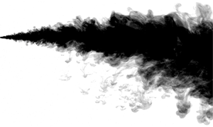
Figure 3 shows a visualisation of a pair of experiments with source Reynolds number  $Re_0=1100$ made using methylene blue dye. The images arranged within the left column, figure 3(a,c,e), show the temporal evolution of a neutrally buoyant single-diffusive freshwater jet, while the right column, figure 3(b,d,f), contains those for an initially neutrally buoyant double-diffusive thermohaline jet. Figures 3(a) and 3(b) demonstrate that both jets became turbulent immediately upon discharge and grew in radius. The shear-induced large-scale turbulent eddies present around the edges of the jets acted to rapidly entrain ambient fluid, which was consequently irreversibly mixed into the core. This turbulent entrainment led to a further growth in jet radius, shown in figures 3(c) and 3(d), as both jets continued to propagate downstream. Although still qualitatively very similar, figure 3(d) shows that 30 s after the ejection, the double-diffusive jet started to develop a slight sinking trajectory and the first hints of small (compared to local jet radius) negatively buoyant structures forming along the lower surface. Taken less than a minute later, the image in figure 3(f) shows that these negatively buoyant structures were able to fully form, separate and fall off downwards from the lower surface of the double-diffusive jet. Such structures were absent along the upper surface of the double-diffusive jet, creating clear asymmetry in the flow. They were also absent in the single-diffusive jet experiment (see figure 3e), with the jet preserving visual symmetry around the centreline throughout the duration of the experiment. We believe that these structures are a result of the salt-fingering instability, and explain the mechanism for their formation below.

Figure 3. A series of images taken for two turbulent jet experiments ejected at the source Reynolds number  $Re_0 = 1100$ and visualised using blue dye. Panels (a,c,e) show the development of a neutrally buoyant jet injected into a quiescent fresh ambient water. Panels (b,d,f) show the development of an initially neutrally buoyant double-diffusive thermohaline jet with source salinity difference $\Delta S_0 = 0.690\%$ and temperature difference $\Delta T_0 = 16.2\,^{\circ }\textrm {C}$, injected into a quiescent fresh ambient water (experiment 4). $(a)$
$(a)$  $t=15\ \textrm {s}$. $(b)$
$(b)$  $t=15\ \textrm {s}$. $(c)$
$(c)$  $t=30\ \textrm {s}$. $(d)$
$(d)$  $t=30\ \textrm {s}$. $(e)$
$(e)$  $t=85\ \textrm {s}$. $(f)$
$(f)$  $t=85\ \textrm {s}$.
In a typical experiment, as the hot and salty jet fluid leaves the nozzle, it immediately finds itself surrounded by fresh and cold ambient fluid and two surfaces with very different dynamics form. The upper surface is in the diffusive regime, since hot and salty jet fluid lies beneath a layer of cold and fresh ambient. In contrast, the lower jet surface is in the salt-fingering regime, as hot and salty jet fluid is atop cold and fresh ambient. Heat and salt exchange occurs across both surfaces, but the mechanisms that govern these exchanges are rather distinct.
Along the upper diffusive surface, heat and salt diffusion act to produce two boundary layers: thermal and saline. As heat diffusion is  $O$(100) times faster than salt, the thermal boundary layer will quickly grow to a critical thickness, leading to the formation of convective heat elements (Howard Reference Howard1964). Taking the values of $g= 10\ \textrm {m}\,\textrm {s}^{-2}$, $\beta _T = 10^{-4}\,^{\circ }\textrm {C}$, $\Delta T = 10\,^{\circ }\textrm {C}$, $\kappa _T = 10^{-7}\ \textrm {m}^{2}\,\textrm {s}^{-1}$ and $\nu = 10^{-6}\ \textrm {m}^{2}\,\textrm {s}^{-1}$, we get the value of the Rayleigh number $Ra=(g \beta _T \Delta T L^3)/(\kappa _T \nu ) \sim 10^{11} L^3$. Then, assuming that turbulent convection ensues for $Ra\sim 10^3$, the critical depth of the thermal boundary layer is $L\sim 10^{-8/3}$. The source temperature differences for most experiments were 2–3 times greater than $10\,^{\circ }\textrm {C}$, therefore let us round to $L\sim 10^{-3}$. Hence, the diffusive growth time of the thermal boundary layer to the critical thickness was $\tau _T=L^2/\kappa _T = O(1)\ \textrm {s}$. The formed convective elements carry away salt, as well as heat, which are consequently irreversibly mixed with the ambient through molecular processes, and the fluid in the jet becomes more dense as a result of the differential loss of heat compared to salt. The dynamics of diffusive interfaces was studied in detail by Turner (Reference Turner1965) and the reader is referred to his work for more detail.
Along the lower surface, heat and salt are exchanged through the jet–ambient interface in a substantially different manner. When a patch of warm and salty jet fluid lying above a layer of cold and fresh ambient is perturbed, the  $O$(100) times faster heat diffusion acts rapidly to adjust the temperature of the perturbed patch towards that of the ambient, while most of its salt is retained. The fluid parcel therefore quickly finds itself denser than its surroundings and starts to sink. The convective elements, formed in this way, will carry heat, as well as salt, as they sink and irreversibly mix with the ambient through molecular diffusion. Owing to their long and thin geometry, such structures are commonly called ‘salt fingers’. In this case the higher salt flux compared to the heat flux, in density terms, results in a decrease in density of the jet. For greater detail on the processes governing the dynamics of a salt-fingering interface, the reader is referred to Turner (Reference Turner1967). Consequently, taken together, the double diffusion over the upper surface of the jet will increase the density of the jet, while over the lower surface of the jet it will decrease the density. The ultimate trajectory of the jet depends on which of these two processes is dominant. We will return to this point in § 3.3.
Figure 4 allows closer visual examination of the temporal evolution of the observed salt fingers for experiment 2. In the early stages of the jet development, there was an absence of ‘clear’ salt-finger structures (shown in figure 4a). Salt fingers began to emerge at a distance beyond  $x/r_0\simeq 100$ as seen in figure 4(b). Indeed, snapshots at later times, see figure 4(a,c,d), show that no fingers form in the region close to the source ( $x/r_0<100$) throughout the entire experiment. Note that this distance varied between different experiments and this will be discussed in detail in § 3.5. Visually it appeared that in many instances salt plumes attempting to form along the lower surface and separate from the jet were not able to do so as they were re-entrained into the jet through the action of turbulent entrainment. This was particularly clear in the region near the source, where turbulent entrainment is the strongest.

Figure 4. Instantaneous images showing the emergence and temporal evolution of salt fingers along the lower jet surface for experiment 2.  $(a)$
$(a)$  $t=10\ \textrm {s}$. $(b)$
$(b)$  $t=35\ \textrm {s}$. $(c)$
$(c)$  $t=70\ \textrm {s}$. $(d)$
$(d)$  $t=200\ \textrm {s}$.
Fingers that managed to detach from the jet, shown in figure 4(c), fall downwards and interact with one another. As the jet propagates, more fingers emerge, forming a persistent ‘rain’ of salt and heat underneath the jet, as shown in figure 4(d). Visual examination of the recorded videos revealed that many fingers formed from turbulent eddies that had been ‘thrown’ out from the jet core by the action of jet-generated turbulence. Once out in the ambient, these eddies were able to rapidly reject their heat, build up negative buoyancy and fall downwards as salt fingers. In cases where the scales of detached eddies were sufficiently large, they broke down into a number of smaller fingers during descent. This observation is consistent with the idea that the horizontal length scale of a salt finger is limited by the competing diffusive processes (Turner Reference Turner1974). In particular, while eddies that are too wide are not able to reject heat effectively, the motion of narrow structures is restrained by viscosity, and therefore fingers exist at intermediate scales.
Ultimately, it is the origin of the observed deviation from a horizontal trajectory, seen clearly in figure 3(e), and the nature of the salt fingers, shown in figure 4, that we aim to investigate further in this study.
3.2. Time-average analysis
Figure 5 shows the time-averaged images for all experiments obtained by averaging over  ${\sim }3000$ snapshots, with the exact quantity for each experiment provided in table 1. These snapshots for time averaging were taken at regular time intervals over the entire duration of the experiment, with the first snapshot taken 2 s after the retraction of the siphon. Note that in all cases, the trajectories of the jets did not vary with time, implying that all jets were in a quasi-steady state. Two observations have to be made at this stage. First, this figure shows that for a given source Reynolds number, as the source temperature difference $\Delta T_0$ increases, the jet horizontal propagation is reduced and a more curved trajectory is observed. Take, as an example, the three experiments performed at $Re_0=700$. Ejected at $\Delta T_0=15.8\,^{\circ }\textrm {C}$, the jet reached the end of the viewing window at $x/r_0\simeq 600$. This distance reduced significantly, to $x/r_0\simeq 400$ and $\simeq 250$, as the source temperature differences increased to $\Delta T_0=25.2\,^{\circ }\textrm {C}$ and $\Delta T_0= 38.3\,^{\circ }\textrm {C}$, respectively. This trend holds consistently for the other two groups with three experiments in each, performed at $Re_0=1100$ and $Re_0=1500$, indicating clearly that double-diffusive processes have a strong impact on the paths followed by the jets. Evidently, the potential for double-diffusive processes to alter the jet trajectory is greater for larger source temperature differences.

Figure 5. Time-average images of the jets for all experiments plotted against source temperature difference (a–c, d–f, g–i) and Reynolds number (a,d,g, b,e,h, c,f,i).
The second trend seen clearly in figure 5 is that for a given source temperature difference, as the source Reynolds number was increased, the jets followed a less curved trajectory. This is consistent with the idea that the momentum flux acts against the negative buoyancy driving the jet downwards. As explained above, this buoyancy is introduced by the action of double-diffusive processes and is controlled by the source temperature difference. The balance between buoyancy-driven velocity and jet velocity is commonly expressed using the densimetric Froude number  $Fr = U/\sqrt {g'L}$, where $U$ is the horizontal velocity scale, $L$ is the characteristic length scale, for example the jet radius, and $g'=g(\rho -\rho _a)/\rho _a$ is the buoyancy scale. Neutrally buoyant jets, for which $Fr \to \infty$, follow a perfectly horizontal trajectory. Buoyant jets with large buoyancy differences and thus low $Fr$ numbers exhibit strongly curved trajectories. In our experiments an increase in the source Reynolds number corresponds to an increase in the source horizontal velocity $U$. For a fixed $\Delta T_0$ the effective Froude number is therefore higher for higher $Re_0$, so as $Re$ is increased, the jet trajectory remains closer to the horizontal. We attempt to explain the origin of the development of negative buoyancy within the jet in the next section.
3.3. Sinking trajectory explanation
One possible explanation for the build-up of negative buoyancy and the observed sinking jet motion is based on the differences in salinity and temperature fluxes across the two double-diffusive surfaces. We denote the double-diffusive temperature and salt fluxes across the upper diffusive surface as  $F^U_T$ and $F^U_S$, respectively. The associated salt-fingering salt and temperature fluxes across the lower surface are denoted as $F^L_S$ and $F^L_T$, respectively. The difference between the net density gain as a result of turbulent diffusive fluxes across the upper surface $F^U_{\rho }$, and the net density loss through the lower fingering surface $F^L_{\rho }$ determines the net density flux from/into the jet and hence the build-up of negative buoyancy. This difference, illustrated pictorially in figure 6, can be written as
 \begin{equation} \frac{F^U_{\rho}}{F^L_{\rho}} = \frac{\beta_T F^U_T - \beta_S F^U_S}{\beta_T F^L_T - \beta_S F^L_S}. \end{equation}
The problem at this stage relies on the accurate determination of the double-diffusive fluxes involved in the process. From dimensional considerations, Turner (Reference Turner1965, Reference Turner1967) showed that for high Rayleigh number diffusive and fingering interfaces, the turbulent fluxes of temperature  $F^U_T$ and salinity $F^L_S$, respectively, can be related to the turbulent fluxes from a ‘solid wall’ (i.e. the fluxes from a fixed temperature/salinity boundary held at a constant temperature/salinity difference from the values in the fluid away from the boundary) as
 \begin{gather} F^U_T = c \kappa_T^{2/3} \left(\frac{\beta_T g}{\nu} \right)^{1/3} \Delta T^{4/3} f(R^*_{\rho}), \end{gather}
 \begin{gather}F^L_S = c \kappa_S^{2/3} \left(\frac{\beta_S g}{\nu} \right)^{1/3} \Delta S^{4/3} f(R_{\rho}), \end{gather}
where  $c$ is an experimentally determined constant and $R^*_{\rho }=1/R_{\rho }$. Turner (Reference Turner1965, Reference Turner1967) measured experimentally over a range of density ratios the numerical coefficients $R_D=f(R^*_{\rho })$ and $R_S=f(R_{\rho })$, which relate the double-diffusive diffusive temperature and salt fluxes to their reference solid wall values, respectively. He also measured how the flux ratios $\gamma _D =(\beta _S F^U_S)/(\beta _T F^U_T)$ and $\gamma _S = (\beta _T F^L_T)/(\beta _S F^L_S)$ for diffusive and salt-fingering interfaces, respectively, vary as a function of the density ratio $R_{\rho }$. Using the above definitions, the ratio of density fluxes in (3.1) can be rewritten as
 \begin{equation} \frac{F^U_{\rho}}{F^L_{\rho}} = \frac{R_D}{R_S} \left(\frac{\kappa_T}{\kappa_S}\right)^{2/3} \left(\frac{1-\gamma_D}{1-\gamma_S}\right) \left(\frac{\beta_T \Delta T}{\beta_S \Delta S}\right)^{4/3}. \end{equation}
Precise calculations of the fluxes require exact measurements of numerical values of the flux coefficients for double-diffusive interfaces in the presence of turbulence, which are not readily available. Another factor complicating the problem is the unknown non-trivial effect of differential diffusion in the presence of turbulence on the evolution of the density ratio  $R_{\rho }$ of a double-diffusive jet. This governs the choice of coefficient values that go into the flux calculations. To get an order of magnitude estimate using Turner's measurements, we take $R_D/R_S=10^{-1}$, $(\kappa _T/\kappa _S)^{2/3}=10$ and $(1-\gamma _D)/(1-\gamma _S)=1$. Using these values, the density flux ratio is $O$(1), implying that it is a delicate balance between the temperature and salinity fluxes that determines the net density flux.

Figure 6. Schematic representation of the double-diffusive thermohaline jet in a stationary uniform freshwater ambient.
Although the precise spatial evolution of the density ratio is unknown, visual observations of the sinking jet trajectories suggest that as the jet propagates its density ratio becomes  $R_{\rho }<1$. Taking as an example the value of $R_{\rho }=2/3$ and substituting the associated coefficient values from Turner's experimental measurements yields a value of $F^U_{\rho }/F^L_{\rho }\simeq 0.8$. Further reduction in $R_{\rho }$ would lead to a further decrease in the density flux ratio, implying that, contrary to our observations, the jets in this configuration should become positively buoyant. This simple balance calculation, however, uses numerical coefficients that do not take into account two important factors: (i) the effect of turbulence on the fluxes across both surfaces; (ii) continued absence of salt fingers close to the source, as shown in figure 4. It is the combined effect of these two factors, that leads to the reversal of flux balance, leading to the development of negative buoyancy.
With respect to the first factor, turbulent motions generated by the jet affect its upper and lower surfaces in two distinct ways. Along the upper diffusive surface, turbulence acts to stretch the interface between the jet and the ambient, continuously sharpening the temperature gradient, and hence leading to an increased diffusive heat flux. The impact of jet turbulence on the dynamics of the lower fingering surface is somewhat more complicated. Linden (Reference Linden1971) investigated experimentally the effect of grid-generated turbulence on heat and salt transport across salt-fingering interface in a two-layered aqueous system. For the purpose of our work we will focus on two of his major findings. First, he showed that turbulent shear disrupts the formation of salt fingers and thus reduces the total salt-fingering flux across an interface. Second, he found that the ratio of buoyancy fluxes  $\gamma _S$ was greater than unity for all the grid frequencies (except zero), reaching up to $\gamma _S\approx 4$ for particularly high intensities of the grid turbulence. This means that the density step between two layers was decreasing with time, that is, the top layer was becoming heavier. Ultimately, this first factor implies that the numerical coefficients used in the above flux calculations, determined from experiments with stationary interfaces, are unlikely to be appropriate for a highly turbulent flow and instead flux ratios favouring greater heat exchange should be used.
The implication of the second factor is, perhaps, even more pronounced. In the absence of salt fingers across the lower surface, the resulting salt flux is significantly reduced, that is,  $F^L_{\rho }\sim 0$. This, in turn, means that thermal exchange through the diffusive surface will be the dominant mechanism, leading to a rapid build-up of negative buoyancy. Diffusive heat exchange will dominate for as long as there are no salt fingers forming, which in our experiments was for at least $x/r_0=40$, as will be shown in § 3.5. By that point, the dilution through entrainment alone will have reduced the jet temperature and salinity to $\simeq 0.2\Delta T_0$ and $\simeq 0.2\Delta S_0$ (Hirst Reference Hirst1971), meaning that although salt fingers will be formed beyond this stage, their impact on the total density flux will be relatively small.
3.4. Centreline analysis
With the aim of demonstrating the significance of diffusive processes on the dynamics of double-diffusive jets, we tracked their time-averaged trajectories. To that end, we processed the normalised time-averaged images to extract centrelines, which were used as proxy for trajectories. Each centreline was constructed as a collection of centrepoints for every pixel column, that is, for every  $x$-coordinate, for a given time-averaged image. A centrepoint was defined as the $y$-location of a pixel with the minimum intensity (corresponding to the darkest point) within a particular column of pixels. Using the above definitions, a one-dimensional array with the locations of all centrepoints was obtained for every time-average image, and used to reproduce centrelines. Figure 7 demonstrates the obtained result for experiment 5, which was typical for all experiments. The figure shows that the centrepoints, shown as bright dots, visually follow well the time-averaged jet image and can be used to approximate the jet trajectory.

Figure 7. Image showing that the centreline follows well the time-average jet trajectory for experiment 5, typical for all experiments.
Figure 8 shows the trajectories for all nine experiments, obtained using the procedure described above, and grouped by the source temperature differences  $\Delta T_0$. The colours of the markers represent the source Reynolds number, with the brighter lines corresponding to higher values of $Re_0$. We approximated the obtained trajectories using a well-established model for single-diffusive negatively buoyant jets, which uses the similarity solutions, developed by Fan & Brooks (Reference Fan and Brooks1969) on the basis of an integral model for incompressible Boussinesq (i.e. density differences are small compared with the ambient) turbulent round buoyant jets in a uniform ambient fluid. The set of governing equations was solved numerically in Matlab using the value of the entrainment coefficient for buoyant jets $\alpha =0.08$ (Carazzo, Kaminski & Tait Reference Carazzo, Kaminski and Tait2006). To approximate the trajectories for three sets of experiments, we varied the source buoyancy flux via the source temperature difference. The numerical solutions, presented as dashed lines in figures 8(a), 8(b) and 8(c) were obtained for temperature differences of $\Delta T^m_0=-0.7\,^{\circ }\textrm {C}$, $\Delta T^m_0=-2.2\,^{\circ }\textrm {C}$ and $\Delta T^m_0=-7.5\,^{\circ }\textrm {C}$, respectively. The trajectories obtained for these three manually selected temperature differences follow well each group of the experimentally obtained trajectories, which leads to three conclusions.

Figure 8. Trajectories for all experiments grouped by the source temperature differences: (a)  $T_0 = 16.0 \pm 0.4\,^{\circ }\textrm {C}$; (b) $T_0 = 25.0 \pm 0.5\,^{\circ }\textrm {C}$; (c) $T_0 = 39.0 \pm 0.9\,^{\circ }\textrm {C}$. The marker colour indicates the source Reynolds number, with the brighter colours corresponding to the larger values of Re 0. The black lines in each plot represent the numerical solution for trajectory of single-diffusive jets at a fixed source temperature difference, and varying source Froude number.
First, the observed sinking trajectories cannot be attributed to an experimental uncertainty, since the already mentioned experimental error in temperature measurements of  ${\pm }0.1\,^{\circ }\textrm {C}$ is significantly less than the temperature difference required to produce the deviations observed in figure 8. Second, the fact that $|\Delta T^m_0|<|\Delta T_0|$ for all groups of experiments implies that we cannot assume that all the heat simply diffused out and the jets were driven by the remaining salt. This suggests that within the measurement range, all jets continued to carry some amount of potential energy stored in the form of heat within them. Third, the fact that a single source buoyancy flux is able to approximate the trajectory so well suggests that the diffusive processes play little role relatively soon after discharge. It follows that accumulation of negative buoyancy of the jet happens rapidly and, once developed, stays relatively constant throughout rest of its propagation. This third conclusion is consistent with the idea of the dominant heat diffusion being responsible for the build-up of negative buoyancy in the absence of salt fingers, as outlined in the previous section. Close to the source, temperature gradients are large, causing vigorous heat exchange with the ambient and resulting in a rapid build-up of negative buoyancy. As the jet propagates, the dilution through entrainment makes these gradients fall, reducing the ability for the diffusive flux to reject heat and thereby accumulate negative buoyancy. As a result, the trajectories followed by the jet are preconditioned by the density excess which is established by strong double-diffusive effects near the source where $\Delta T$ and $\Delta S$ are both large. This explains the observation that jets reached a quasi-steady state and followed the same trajectory throughout an experimental run.
3.5. The onset of salt fingers
We now return to the discussion on the development of the salt fingers. As described in § 3.1, visual observations indicate the presence of a competition between the diffusive processes driving the formation of salt fingers and the entrainment acting to inhibit their separation from the jet. We propose that it is the balance between the two competing velocity scales, the salt-fingering velocity  $w_f(x)$ and entrainment velocity $u_e(x)$, that determines the location $x_f$ of the onset point for fingering formation, and provide experimental evidence in support of this hypothesis.
For an axisymmetric turbulent round jet emanating from a point source of momentum, using the entrainment assumption (Morton, Taylor & Turner Reference Morton, Taylor and Turner1956), the expression for the centreline horizontal velocity as a function of distance travelled by the jet can be written as
 \begin{equation} U(x) = \frac{1}{\sqrt{2}\alpha} U_0\frac{r_0}{x}. \end{equation}
Given that  $U(x)$ decays as $x^{-1}$ with distance, so does the jet entrainment velocity $u_e(x) = \alpha U(x)$, indicating that the ability for the jet to re-entrain the salt fingers reduces rapidly with distance. In contrast, the diffusive nature of salt fingers suggests that their velocity scale $w_f(x)$ should be some growing function of time, or in this case distance along the jet. By considering a balance between thermal diffusion and viscosity, Linden (Reference Linden1971) constructed the salt-fingering velocity scale of the form
 \begin{equation} w_f(x) = \frac{g l^2(x) \beta_S \Delta S(x) (\gamma_S-1)}{2\nu{\rm \pi}^2}, \end{equation}
where  $l(x)$ and $\Delta S(x)$ are the finger horizontal length scale and salinity scale, respectively. Visual observations of salt fingers in our experiments showed that they often emerged from turbulent eddies, with their size growing with distance from the source. Burridge, Partridge & Linden (Reference Burridge, Partridge and Linden2016) showed that in a turbulent plume, the length scale of the largest turbulent eddies is 0.44 times its local half-width $r(x)$. Given the similarity in the turbulent properties between jets and plumes, as demonstrated by Van Reeuwijk et al. (Reference Van Reeuwijk, Salizzoni, Hunt and Craske2016), and assuming that the length scales of salt fingers are directly linked to that of the turbulent eddies, we take $l(x) = 0.44\, r(x)$. We assume that the salinity profile matches that of velocity, that is
 \begin{equation} S_m(x) = \frac{1}{\sqrt{2}\alpha} S_0\frac{r_0}{x}, \end{equation}
and take the top-hat values  $\Delta S(x)=S_m(x)/2$ to describe the salinity scale of the fingers.
Using the above definitions, it is possible to predict the fingering onset location  $x_f$ by determining where the two velocity scales become comparable $w_f(x_f) = u_e(x_f)$, as illustrated pictorially in figure 9. In this figure, the dark and bright solid lines represent the entrainment and salt-fingering velocity scales, respectively, with the locations where the two velocity scales reach a balance ( $x_f$) marked using black dots and connected dashed lines. This balance was considered for two distinct cases. In the first case, shown in figure 9(a) we fixed the source salinity $\Delta S_0$ and varied $Re_0$. The source values used in this model were taken as those for experiments 1, 4 and 7, allowing us to compare the obtained predictions against the experiments. The model predicts that an increase of $Re_0$ results in a delay in the formation of salt fingers, consistent with our qualitative observations. For the second case, shown in figure 9(a), we fixed the source Reynolds number $Re_0$ and varied $\Delta S_0$, using the source values for experiments 1, 2 and 3. As expected, for larger source salinity, the velocity scales of salt fingers are larger, resulting in the earlier formation of the salt fingers. To check the validity of the proposed balance between the two competing velocity scales, we compared the obtained predictions against the visual measurements of the onset of salt fingers, obtained using the procedure described below.

Figure 9. Fingering onset prediction for two cases:  $(a)$ at fixed source salinity $\Delta S_0$ and varying $Re_0$ using source values for experiments 1, 4 and 7, with the upper lines corresponding to the larger values of $Re_0$; $(b)$ at fixed source Reynolds number $Re_0$ and varying $\Delta S_0$ using source values for experiments 1, 2 and 3, with the upper lines corresponding to the larger values of $\Delta S_0$. The black dots and connected dashed lines indicate the distance from the source $x_f$ where the first salt fingers should form.
Detection of the salt fingers was performed by temporal sampling of the instantaneous jet images along the so-called ‘gate lines’, with an example represented by the dotted lines in figure 10. The choice of the term ‘gate’ is arbitrary, and was adopted to signify that only those structures which were able to cross the ‘gate’ were considered. Such gate lines were obtained individually for every experiment from their respective time-averaged images using the following procedure. As a first step, we extracted the centreline, as described earlier, and approximated it using a third-order polynomial least-squares fit. We chose to approximate the measured centreline using a polynomial to both smooth the data and to easily find the derivative of the function defining the centreline. Using polynomials of higher orders did not make a noticeable difference to the obtained trajectory and therefore the third order was deemed sufficient. We checked that the obtained fittings, with a typical example shown as a dashed line in figure 10(a), displayed a satisfactory agreement with the centreline points and visually followed the time-averaged jet trajectories well. For the next step, we detected the top edge of the time-averaged jet image. This was done by first filtering out any noise from the image using a single threshold value (signal below a threshold value was considered noise and removed) and then detecting the positions where the intensity changed abruptly within every pixel column. The threshold value was set as the average plus two standard deviations of the value of the ambient measured in absence of any flow. Using the derivative of the centreline position, the upper edge was located by searching on a line perpendicular to the centreline until the upper edge was located. The obtained upper edge was then mirrored perpendicularly around the centreline to create a lower interface (shown as a solid line below the centreline), which could not be otherwise detected due to the presence of salt fingers. The gate line was then constructed by scaling the bottom edge by a fixed multiple of the local jet radius. As can be seen in figure 10(b), the jet width fluctuates about the time-average envelope. For this reason, and to avoid detecting intermittent events that remain attached to the plume, we choose the scaling factor to be  ${\times }2$, meaning that any structure found more than one radius away from the time-averaged bottom edge is considered to be a finger that has managed to escape the re-entrainment process, rather than a turbulent eddy. Figure 10(b) shows an overlay of the obtained lines onto an instantaneous image from experiment 5. The figure shows that for this particular instance, the gate line will not pick up any signal of salt fingers until up to $x/r_0\simeq 80$ and will have a strong signal of the presence of salt fingers thereafter until $x/r_0\simeq 350$. The region $x/r_0\simeq 350$ and $x/r_0\simeq 380$ will once again contain no salt-fingering signal.

Figure 10. An illustration of the ‘gate line’ construction procedure and application:  $(a)$ gate line construction using the time-averaged image for experiment 5; $(b)$ an overlay of the centreline, edges and the gate line onto an instant capturing salt fingers crossing the gate line. In both panels, the centreline fit is represented by the dashed line, the edges are represented by the solid lines and the dotted line represents the gate line. The arrow in $(a)$ represents the local jet coordinate system.
Figures 11 and 12 show the obtained time series of the jet images, sampled along the gate lines as described above. In line with the visual observation made in figure 4, both figures show that in all cases there were consistently no fingers forming until some distance away from the source, which varied between experiments. The dashed vertical lines present in all figures are the predictions made using the model described above and shown in figure 9. As seen in figure 11, experimental results are in good agreement with the model prediction, confirming that the formation of salt fingers is delayed as the source Reynolds number is increased. Similarly, there seems to be a good agreement between the predicted and observed onset points for a fixed  $Re_0$ and varying $\Delta T_0$ (see figure 12). As expected, the formation of salt fingers is earlier for larger values of $\Delta T_0$, that in our experiments is equivalent to larger values of $\Delta S_0$. These two observations confirm that it is the balance between the double-diffusive processes and turbulent entrainment that controls the formation of salt fingers in a horizontal jet.

Figure 11. Time series of dye concentration profiles taken along the gate lines for three experiments at fixed  $\Delta T_0=15\pm 0.4\, ^{\circ }\textrm {C}$. The dashed lines represent the prediction for the fingers onset location $x_f$ for respective source conditions shown in figure 9(a). $(a)$
$(a)$  $Re_0 = 700$. $(b)$
$(b)$  $Re_0 = 1100$. $(c)$
$(c)$  $Re_0 = 1500$.

Figure 12. Time series of dye concentration profiles taken along the gate lines for three experiments at fixed  $Re_0=700$. The dashed lines represent the prediction for the fingers onset location $x_f$ for respective source conditions shown in figure 9(b). $(a)$
$(a)$  $\Delta T_0=15.8\,^{\circ }\textrm {C}$. $(b)$
$(b)$  $\Delta T_0=25.2\,^{\circ }\textrm {C}$. $(c)$
$(c)$  $\Delta T_0=38.3\,^{\circ }\textrm {C}$.
4. Conclusions
An experimental investigation of the effect of double diffusion on the dynamics of turbulent jets has been conducted. We have restricted our attention to the simplest case of initially neutrally buoyant thermohaline jets discharged horizontally into a stationary uniform freshwater ambient. Visual observations revealed that, in contrast to their freshwater equivalents, neutrally buoyant double-diffusive jets develop considerable sinking trajectories, with significant salt-fingering convection forming along the lower jet-ambient surface some considerable distance away from the source. The tendency for the jets to sink is greater for larger source temperature differences  $\Delta T_0$, demonstrating the significance of double-diffusive processes for turbulent jet motion.
We associate the observed sinking trajectories with the impact of internal jet-generated turbulence on the fluxes of heat and salt across its upper and lower surfaces. Importantly, turbulent entrainment hinders the formation of the salt fingers for a considerable distance from the jet source. In the absence of advective salt transport through salt-fingering motion, the diffusive heat losses dominate, resulting in the build-up of negative buoyancy which drives the jet downwards. Note that other effects, such as the impact of salt-fingering motion on the turbulent entrainment processes along the lower surface of the jet, could be partially responsible for the observed sinking behaviour. However, given that we were able to explain our results without involving any additional effects, we feel that they are likely to be at best of secondary importance to the double-diffusive processes.
Double-diffusive jet trajectories can be well approximated by a trajectory of a single-diffusive buoyant jet with a fixed source buoyancy  $g_0'$, indicating that accumulation of negative buoyancy happens quickly, since otherwise the diffusive processes would continuously change the jet buoyancy and hence trajectory. In addition, a simple model predicting the onset point of the salt fingers works well by balancing entrainment and salt-fingering velocity scales, confirming our physical understanding of the formation of salt fingers in this context.
This work has important modelling implications for industrial discharges involving double-diffusive jets, such as the brine discharges from desalination plants. First, it shows that using the standard single-diffusive buoyant jet equations for the case of thermohaline double-diffusive discharges may lead to a significant underestimation of the curvature of jet trajectory, overpredicting the distance travelled by the effluent, and consequently its dilution. Such models should therefore be used with caution. The second implication concerns various chemicals, such as copper and chlorine, added to the seawater at different stages in the desalination process to control bacterial growth and/or reduce corrosion (Jones et al. Reference Jones, Qadir, van Vliet, Smakhtin and Kang2019). Based on our results, it is likely that instead of propagating with the jet (going through continuous dilution to low concentrations through entrainment), these slow-diffusing chemicals may tend to fall out in the form of salt fingers, causing additional pollution in the near-coastal region, which is unaccounted for by the current single-diffusive models.
Finally, in addition to the recent work by Dadonau et al. (Reference Dadonau, Partridge and Linden2020), this investigation provides a further confirmation that for high-Péclet-number flows, in which advection dominates diffusion, diffusive processes may have a considerable impact on the large-scale dynamics of turbulent free shear flows, as well as on the structure of the turbulent/non-turbulent interface.
Acknowledgements
We acknowledge funding from the EPSRC under the Programme Grant EP/K034529/1 ‘Mathematical Underpinnings of Stratified Turbulence’ (MUST), and from the European Research Council (ERC) under the European Union's Horizon 2020 research and innovation programme under grant No 742480 ‘Stratified Turbulence And Mixing Processes’ (STAMP). M.D. is supported by the Gates Cambridge Scholarship. We are grateful for the invaluable experimental support of Professor S. Dalziel and of the technicians of the G. K. Batchelor Laboratory.
Declaration of interests
The authors report no conflict of interest.


 Open access