


1. Introduction
Fluid instabilities or hydrodynamic instabilities form an important pillar of fluid mechanics, and are one route by which a system can transition to a turbulent state. Instability-induced turbulent mixing is found in many natural phenomena and engineering applications, and covers a wide range of length and time scales. Instability-driven flows are often encountered in atmospheric and oceanic flows (Lyons, Panofsky & Wollaston Reference Lyons, Panofsky and Wollaston1964; Browand & Winant Reference Browand and Winant1973; Turner Reference Turner1980; Wilcock & Whitehead Reference Wilcock and Whitehead1991; Werne & Fritts Reference Werne and Fritts1999; Kelley et al. Reference Kelley, Chen, Beland, Woodman, Chau and Werne2005), combustion chambers (Nagata & Komori Reference Nagata and Komori2000), inertial confinement fusion (ICF) targets (Sharp Reference Sharp1984) and supernova collapse and explosion (Hachisu et al. Reference Hachisu, Matsuda, Nomoto and Shigeyama1991; Burrows Reference Burrows2000; Musci et al. Reference Musci, Petter, Pathikonda, Ochs and Ranjan2020).
A frequently encountered instability is the buoyancy-driven Rayleigh–Taylor instability (RTI) which affects the interface of fluids where the pressure gradient and density gradient are misaligned such that  $\boldsymbol {\nabla } p \boldsymbol{\cdot} \boldsymbol {\nabla } \rho < 0$. Vorticity is deposited at such an interface and small perturbations therein grow with time due to the baroclinic vorticity production term ( ${\sim }\boldsymbol {\nabla }\rho \times \boldsymbol {\nabla }p$) in the vorticity transport equation. Most often (as in the current study) the pressure gradient is due to gravity $g$ under hydrostatic conditions. The density difference between the two fluids is indicated by a dimensionless number called the Atwood number $\mathcal {A}$, defined by
 \begin{equation} \mathcal{A} = \frac{\rho_1 - \rho_2}{\rho_1 + \rho_2}, \end{equation}
where  $\rho _1$ is the density of the heavier, top fluid and $\rho _2$ is the density of the lighter, bottom fluid, making the two fluids system initially unstable.
It is convenient to break the growth regimes of the RTI with multimodal initial perturbations into four stages (Lewis Reference Lewis1950; Birkhoff Reference Birkhoff1955; Sharp Reference Sharp1984; Youngs Reference Youngs1984). In the first stage, perturbations (with amplitudes much smaller than their wavelengths) grow exponentially with growth rate proportional to  $\sqrt {\kappa g \mathcal {A}}$ (where $\kappa$ is the spatial wavenumber of the perturbation) according to linear stability theory (Taylor Reference Taylor1938). Here, in the linear regime, small wavelength perturbations grow exponentially faster than large wavelength perturbations (Sharp Reference Sharp1984; Drazin & Reid Reference Drazin and Reid2004). As the perturbation amplitude becomes comparable to the wavelength, the instability enters the second stage where the growth of small wavelength perturbations saturate (Lewis Reference Lewis1950) while larger wavelength perturbations continue to grow, causing large structures to appear in the flow. These structures take on the appearance of alternating and interpenetrating bubbles of rising light fluid and spikes of falling heavy fluid. In the third stage, nonlinear interaction between bubbles and spikes continues. These structures compete with each other, causing them to reduce in size (for example, due to shear instabilities and dissipation), or can merge to generate larger structures (like bubble amalgamation) (Li Reference Li1996). In the final, fourth stage, RTI structures break up by different means, like shear and interpenetration. This stage is characterized by turbulent mixing. Experiments in this regime (Read Reference Read1984) show that the half-width of the mixing region, $h_{RT}$, grows quadratically in time $t$, as given by (1.2):
 \begin{equation} |h_{RT,b,s}| = \alpha_{b,s} \mathcal{A} g t^2, \end{equation}
where  $h_{RT} = (|h_{RT,b}| + |h_{RT,s}|)/2$, $|h_{RT,b}|$ is the magnitude of the bubble height, $|h_{RT,s}|$ is the magnitude of the spike height, $\alpha _b$ is the bubble growth-rate parameter, and $\alpha _s$ is the spike growth-rate parameter. This relationship has been established through other analyses as well, specifically through Lagrangian analysis (Fermi & Neumann Reference Fermi and Neumann1955), modelling of turbulent mixing (Birkhoff Reference Birkhoff1955), physical arguments along with linear stability results (Youngs Reference Youngs1984), self-similar analysis of the Navier–Stokes equations (Ristorcelli & Clark Reference Ristorcelli and Clark2004) and a mass flux and energy balance (Cook, Cabot & Miller Reference Cook, Cabot and Miller2004). The half-width of the mixing region $h_{RT}$ can also be written as $h_{RT} = \alpha \mathcal {A} g t^2$, where $\alpha$ is the average of the bubble and spike growth-rate parameters. For moderately high density differences with $\mathcal {A} > 0.2$, the growth-rate parameters for bubble and spike need not be equal (Akula & Ranjan Reference Akula and Ranjan2016), and one deals with separate growth-rate parameters, $\alpha _b$ for bubble growth and $\alpha _s$ for spike growth. Experiments and numerical simulations have shown a wide range in values of $\alpha _b$, from 0.02 to 0.08, depending on the density ratio, accelerations and initial perturbations (Dimonte et al. Reference Dimonte, Youngs, Dimits, Weber, Marinak, Wunsch, Garasi, Robinson, Andrews and Ramaprabhu2004).
Many RTI experiments have been performed in a box-type set-up in which fluids of different densities are placed one above another, and these experiments are transient in nature with very short experimental times. In some of these experiments, the fluids are initially placed in a stably stratified configuration (i.e. light fluid over heavy fluid) and the container is accelerated in the downward direction with an acceleration magnitude greater than the acceleration due to gravity. This provides a body force in the direction opposite to gravity and thus, RTI develops. Various sources of this acceleration have been used in experiments, such as compressed air to accelerate the liquid column above air (Lewis Reference Lewis1950), rubber tubing and steel wire (Emmons, Chang & Watson Reference Emmons, Chang and Watson1960), bungee cords (Ratafia Reference Ratafia1973), compressed air (Cole & Tankin Reference Cole and Tankin1973), weight pulley drop tower (Waddell, Niederhaus & Jacobs Reference Waddell, Niederhaus and Jacobs2001), rocket rig motors (Read Reference Read1984), linear electric motor (Dimonte & Schneider Reference Dimonte and Schneider1996) and high-pressure gas systems (Kucherenko et al. Reference Kucherenko, Balabin, Ardashova, Kozelkov, Dulov and Romanov2003). Dalziel (Reference Dalziel1993) used a rigid barrier to separate the fluids in an unstable configuration, and the removal of this barrier caused additional initial perturbations in the flow. White et al. (Reference White, Oakley, Anderson and Bonazza2010) used a paramagnetic substance in a strong magnetic field to place the fluids in an unstable configuration.
A convective type system was first used by Snider (Reference Snider1994) to study RTI mixing, and experiments with such a system are statistically stationary in nature. Snider (Reference Snider1994) used hot and cold water to study RTI mixing at small Atwood numbers ( $\mathcal {A} < 10^{-3}$). In this system, the fluid streams, initially separated by a splitter plate, flow at constant velocity before they start to mix at the edge of the splitter plate. Taylor's frozen turbulence hypothesis (Taylor Reference Taylor1938; Pope Reference Pope2000) was used, assuming that the turbulence as well as flow phenomena are convected downstream at constant velocity equal to the stream velocity. In contrast to box-type or transient set-ups, this convective type system allows for larger data sampling times and thus, statistically stationary experiments. A typical experiment can last up to a few minutes, giving enough time to collect turbulent velocity and density statistics at any point in the flow. Snider & Andrews (Reference Snider and Andrews1994) performed back-lighting experiments to obtain mixing width growth rates. Ramaprabhu & Andrews (Reference Ramaprabhu and Andrews2004) made particle image velocimetry (PIV) measurements for the first time inside a RTI mixing layer using a water channel. They used a PIV-scalar technique (Ramaprabhu & Andrews Reference Ramaprabhu and Andrews2003) to make simultaneous measurements of turbulent velocity and density statistics at $\mathcal {A} \approx 2.4 \times 10^{-4}$. Mueschke, Andrews & Schilling (Reference Mueschke, Andrews and Schilling2006) quantified the initial velocity and density profiles right after the splitter plate in the water channel using PIV-scalar as well as thermocouple measurements.
The idea of convective type or statistically stationary systems was extended to develop a gas tunnel facility (Banerjee & Andrews Reference Banerjee and Andrews2006) to study RTI in gases. Air is used for the heavier top stream and air–helium mixture is used for the bottom stream. The Atwood number is varied by changing the amount of helium in the air–helium mixture. Banerjee & Andrews (Reference Banerjee and Andrews2006) used a backlit transparent test section with digital imaging techniques (similar to the water channel) to measure mixing widths at different Atwood numbers. Banerjee, Kraft & Andrews (Reference Banerjee, Kraft and Andrews2010) used a multiposition multioverheat hotwire technique to measure different turbulence quantities across the mixing layer, including the vertical velocity fluctuation  $\overline {v'^2}$, density variance $\overline {\rho '^2}$, streamwise velocity fluctuation $\overline {u'^2}$, and turbulent mass fluxes $\overline {\rho 'u'}$, $\overline {\rho 'v'}$. Kraft, Banerjee & Andrews (Reference Kraft, Banerjee and Andrews2009) developed a new hotwire technique, simultaneous three wire cold wire anemometry (S3WCA), for measuring velocity and density fluctuations separately and simultaneously using the temperature as a marker for density.
Akula (Reference Akula2014) and Akula & Ranjan (Reference Akula and Ranjan2016) improved upon the design of the gas tunnel facility used by Banerjee & Andrews (Reference Banerjee and Andrews2006) and Banerjee et al. (Reference Banerjee, Kraft and Andrews2010), allowing the measurement of RTI turbulent mixing at  $\mathcal {A} = 0.73$. This was done with the introduction of a larger test section, a stronger fan to obtain higher convective speeds and an improved helium injection system. By implementing planar PIV, velocity profiles could be computed across the entire mixing region. They used the S3WCA technique and a newly developed hotwire-based density probe (Akula Reference Akula2014; Akula & Ranjan Reference Akula and Ranjan2016) to make simultaneous velocity–density point measurements, and calculate velocity–density cross-statistics and turbulent mass fluxes $\overline {\rho 'u'}$, $\overline {\rho 'v'}$. The vertical turbulent mass flux $\overline {\rho 'v'}$ is the dominant term and a primary driver of Rayleigh–Taylor turbulence. Mikhaeil (Reference Mikhaeil2020) and Mikhaeil et al. (Reference Mikhaeil, Suchandra, Ranjan and Pathikonda2021) further modified the gas tunnel of Akula (Reference Akula2014) and Akula & Ranjan (Reference Akula and Ranjan2016) to implement laser induced fluorescence (LIF) and used PIV-LIF to obtain simultaneous velocity–density line measurements in low Atwood number RTI-affected flows. These simultaneous measurements gave a deep insight into turbulent kinetic energy transport equation budget for RTI-affected flows. More details on recent advancements in the study of instability-driven flows (particularly RTI-affected flows) can be found in Zhou (Reference Zhou2017a,Reference Zhoub), Banerjee (Reference Banerjee2020), Schilling (Reference Schilling2020), Mikhaeil (Reference Mikhaeil2020), Mikhaeil et al. (Reference Mikhaeil, Suchandra, Ranjan and Pathikonda2021) and Suchandra (Reference Suchandra2022).
Some recent studies (Jacobs & Dalziel Reference Jacobs and Dalziel2005; Wykes & Dalziel Reference Wykes and Dalziel2014) have looked at the interaction between two fluid interfaces, one unstable affected by RTI and other stable. For such a configuration, it is important to study how instability-induced turbulence at one interface affects the entrainment through the otherwise stable neighbouring interface. These kinds of flows form the basis of more complex stratified flows often found in deep layers of oceans. Such multilayer instabilities are also encountered during the implosion process of multilayered ICF capsules. One important aspect to investigate here is to look at the overall growth of the mixing region and to check if this growth is self-similar (and under what conditions).
Jacobs & Dalziel (Reference Jacobs and Dalziel2005) investigated the effect of introducing a third layer to the standard two-layer Rayleigh–Taylor problem but restricted themselves to the Boussinesq limit where the density differences were small compared with the densities (typically,  $\mathcal {A} \ll 1$). The three layers had densities $\rho _1, \rho _2$ and $\rho _3$ from top to bottom, with the upper interface of the middle layer statically unstable ( $\rho _1 > \rho _2$) and lower interface statically stable ( $\rho _2 < \rho _3$). The middle layer thickness $G$ was kept much less than the thicknesses of the top and bottom layers. The upper unstable interface is characterized with Atwood number ${\mathcal {A}}_{12} = (\rho _1 - \rho _2)/(\rho _1 + \rho _2)$. Miscible liquids (fresh water and salt solutions) were used in their experiments, giving Atwood numbers of the order of $10^{-3}$. Planar fluorescence techniques were used for flow visualization (Dalziel, Linden & Youngs Reference Dalziel, Linden and Youngs1999). Their fluorescence image sequences revealed expected results, like increasing the bottom layer density, $\rho _3$, reduced the distortion of lower interface due to RT spikes coming from the RT unstable upper interface. Decreasing the bottom layer density, $\rho _3$, below the top layer density, $\rho _1$, caused the mixing region to evolve like classic RT instability at late times. The authors also presented a self-similarity analysis for the case of $\rho _1 = \rho _3$, assuming a middle layer thickness much smaller than the top and bottom layers, and assuming the Boussinesq limit, i.e. ${\mathcal {A}}_{12} \rightarrow 0$. They found the width of the mixing region, $h_3$, to grow linearly with time, $t$, at late stages of the mixing process, given by
 \begin{equation} h_3 \approx \gamma (\sqrt{{\mathcal{A}}_{12} g G}) t, \end{equation}
where  $\gamma$ is a constant found to be $\approx 0.5$ from their experiments. Note that the mixing width growth here is dependent on the middle layer thickness $G$.
$G$.
The current work aims to experimentally study fluid dynamics and mixing due to multilayer Rayleigh–Taylor instability where a thin light fluid layer is surrounded by heavier fluid layers from top and bottom. Our multilayer RTI experiments are outside the Boussinesq limit, at Atwood numbers  $\mathcal {A} \sim 0.3$ and $0.6$, for which analytical solutions are hard to obtain. In addition to measurements of turbulence statistics, the current work aims to address questions regarding the self-similarity, scaling, energetics and molecular mixing in multilayer RTI.
2. Experimental facility and diagnostics
2.1. Experimental facility
Multilayer RTI experiments are performed using a newly built gas tunnel facility as shown in figure 1. Density stratification is achieved by injecting helium (or a helium–nitrogen mixture) and mixing it with air in the desired stream(s) through a light gas injection system. Three independently controlled fans, located upstream of the test section, are used to control the speeds of the three streams, as shown in figure 1(a). Two sets of adjustable splitter plates, as shown through the cut-out in figure 1(b), allow experiments with different middle layer thickness  $G$. All experiments presented in this paper are done at $G \approx 3$ cm. We have three test sections of identical dimensions (each test section with dimensions as shown in figure 1a) connected in series, giving the total effective test section length of 3.6 m (with a cross-section of $0.6\,{\rm m} \times 0.4\,{\rm m}$). Upon entering the test section, the upstream divisions (splitter plates) between the streams are absent, and the streams start mixing. Measurements can be taken in the test section through visualization techniques (backlit visualization and planar Mie scattering), PIV and planar laser induced fluorescence (PLIF). These experiments are statistically stationary, allowing long data collection times, facilitating measurement and computation of higher-order moments, probability density functions (p.d.f.), and correlations of density and velocity. In such a convective type system, Taylor's frozen turbulence hypothesis (Taylor Reference Taylor1938; Pope Reference Pope2000) is assumed to relate instability development time $t$ with streamwise distance from the splitter plate $x$ using $t = x/U_c$ where $U_c$ is the mean of the convective speed of the flow streams as they enter the test section. The origin of the coordinate system used in this paper (figure 2) is at midway between the two splitter plates (placed $G$ distance apart). The $x$ coordinate runs horizontally along the direction of flow (streamwise direction), the $y$ coordinate runs vertically upward (cross-stream direction), and the $z$ direction runs perpendicular to the other two directions out of the plane of the figure (spanwise direction). Here $u$,
$u$,  $v$ and $w$ denote velocity components along $x$,
$x$,  $y$ and $z$ coordinates, respectively, with $\bar {U}$ or $\bar {u}$ denoting mean component of the velocity and $u'$ denoting the fluctuating component, and so on.

Figure 1. Model of the blow-down three-layer gas tunnel, used for multilayer RTI studies.

Figure 2. Basic flow schematic for multilayer RTI experiments, along with the coordinate system.
The previous gas tunnel used (in Akula & Ranjan Reference Akula and Ranjan2016; Akula et al. Reference Akula, Suchandra, Mikhaeil and Ranjan2017; Mikhaeil Reference Mikhaeil2020; Mikhaeil et al. Reference Mikhaeil, Suchandra, Ranjan and Pathikonda2021) limits data collection and is limited in performance for a number of reasons. Several of those reasons, along with the advantages offered by the new three-layer gas tunnel, are addressed here.
(i) Use of a single fan with manual sliding grates and louvers makes it difficult to control stream speeds in the suction-type tunnel. Use of independently controlled blow-down fans in the blow-down three-layer tunnel makes it easier to control individual stream speeds.
(ii) The blow-down three-layer tunnel has an area contraction ratio of ${\sim }7$ as opposed to the contraction ratio of ${\sim }2.5$ provided by the suction-type tunnel. This results in a well-conditioned uniform flow in the test section of the blow-down three-layer tunnel (Bell & Mehta Reference Bell and Mehta1990; Barlow, Rae & Pope Reference Barlow, Rae and Pope1999; Owen & Owen Reference Owen and Owen2008).
(iii) The test section of the blow-down three-layer tunnel exits into the environment. This is based on the design of the mixing layer wind tunnel of Bell & Mehta (Reference Bell and Mehta1990) and this design ensures maintenance of a roughly uniform, atmospheric pressure at the exit of the test section. This uniform pressure helps avoid any drastic turning/rising of the light middle stream.
(iv) A smaller tunnel and test section significantly reduces the required flow rates of helium gas, fog/oil particles (for planar Mie scattering and PIV) and tracers (like acetone vapor) for LIF-based diagnostics. This makes experiments more economical, significantly increases the experimental times (thus more data of statistical importance) and helps expand diagnostics capabilities.


More details about this gas tunnel along with the details about the light gas injection system can be found in Suchandra (Reference Suchandra2022).
2.2. Scales for imaging diagnostics
The relevant length scales expected to be present in the new three-layer blow-down facility are estimated here. Similar methodology is presented in Mikhaeil (Reference Mikhaeil2020). The outer length scale of the flow is of the order of the mixing width and the fluctuating velocity scale is assumed to be of the order of the mixing width growth rate. To estimate these, self-similar growth of the mixing width is assumed. Taking the time derivative of the self-similar three-layer growth rate in (1.3), the total mixing region growth rate is written as  ${\dot {h}}_{3} = \gamma (\sqrt {{\mathcal {A}}_{12} g G})$. With estimates of $\gamma \sim 0.5$, target Atwood numbers of ${\mathcal {A}}_{12} \sim 0.3$ and ${\mathcal {A}}_{12} \sim 0.6$, gravitational acceleration $g = 9.81\,{\rm m}\,{\rm s}^{-2}$ and relevant thermophysical properties (Wilke Reference Wilke1950), we arrive at estimates for the outer scale Reynolds number ${Re}$ (also referred to as mixing Reynolds number (Dimotakis Reference Dimotakis1991)) for our flows as given by ${{Re}}_{{\dot {h}}_{3}} = {h_{3} {\dot {h}}_{3}}/{\nu _{mix}}$ where mixing width is the relevant length scale and kinematic viscosity of the gas mixture $\nu _{mix}$ is calculated using the approach of Wilke (Reference Wilke1950). These estimates, corresponding to the two streamwise locations $x_1$ and $x_2$ (thus, two time instants in the instability development) for each Atwood number ${\mathcal {A}}_{12}$, are reported in table 1. Note that the higher ${Re}$ at the same ${\mathcal {A}}_{12}$ corresponds to the farther downstream streamwise location (later time in instability development). Note that the subscript ${\dot {h}}_{3}$ in ${{Re}}_{{\dot {h}}_{3}}$ is to emphasize that this estimation of mixing Reynolds number is based on the assumption that the fluctuating velocity scale is of the order of the mixing width growth rate. Later in the paper when discussing the results, the mixing Reynolds number based on measured velocity fluctuations is calculated and it is referred to as ${{Re}}_{v'}$.
Table 1. Estimates of the mixing Reynolds number  ${Re}$, Kolmogorov microscale $\eta$ and Taylor microscale $\lambda _T$ predicted for this multilayer RTI study.

Turbulent flows manifest a range of length scales, thus other relevant length scales beyond the mixing width should be considered. The Kolmogorov microscale  $\eta$ is the smallest scale at which viscosity dissipates mechanical energy of the fluid motion into heat. Using the dimensional analysis as suggested in Tennekes & Lumley (Reference Tennekes and Lumley1972) and Pope (Reference Pope2000), estimates of the Kolmogorov microscale are given by $\eta = h_{3} {{Re}}^{-3/4}$ and reported in table 1. The Taylor microscale $\lambda _T$ is another important length scale for turbulent flows. It is an intermediate length scale, between the outer length scale (mixing width) and the Kolmogorov microscale, at which viscosity significantly affects the dynamics of turbulent eddies in the flow (Tennekes & Lumley Reference Tennekes and Lumley1972). Like the Kolmogorov microscale, dimensional arguments (Tennekes & Lumley Reference Tennekes and Lumley1972; Pope Reference Pope2000) can be used to find an estimate for the Taylor microscale in terms of the mixing width and mixing Reynolds number, given by $\lambda _T = h_{3}\sqrt {10} {{Re}}^{-1/2}$ and reported in table 1. The measurement of the Taylor microscale in the flow is important to check if there is enough separation between different length scales (mixing width versus Taylor microscale versus Kolmogorov microscale) and if the flow transitions to a turbulent state (Tennekes & Lumley Reference Tennekes and Lumley1972; Pope Reference Pope2000; Mikhaeil Reference Mikhaeil2020). Therefore, it is vital that our measurement diagnostics resolve the Taylor microscale.
2.3. Backlit visualization and planar Mie scattering
Here, flow visualization techniques are used to estimate the width of the mixing region in the flow, and to get a sense of the mean density distribution. The test section is lit from one side using an array of light emitting diode (LED) panels. A large sheet of matt acetate paper is placed between the light panels and the test section to ensure diffuse and uniform illumination of the flow. One of the fluid streams (middle layer most of the time) is seeded with Master FX $\unicode{x00AE}$ code 6 platinum water-based fog particles of size in the range 10– $50\,\mathrm {\mu }$m. The seeded layer acts as a thin light-extinguishing medium, and the absorption of light due to the presence of the fog is linearly proportional to the volume fraction of fog, as approximated from Beer–Lambert's law (Akula, Andrews & Ranjan Reference Akula, Andrews and Ranjan2013). Images of the flow are then collected using an SLR camera (Nikon $\unicode{x00AE}$ D90/D4 camera), and pixel intensity is mapped to volume fraction. These images are processed through a background subtraction technique to remove non-uniformities, and are then ensemble-averaged. We then use the intensity values from this averaged greyscale image to get the mixing width as discussed in the results § 3.
Another visualization technique used is based on planar Mie scattering of laser light off of fog particles. The overall image acquisition and processing procedure is the same as the backlit visualization described before (laser firing and image capture are synced). In addition to background subtraction, the planar Mie scattering images are also corrected for the divergence of laser sheet. The main difference between the backlit visualization and planar Mie scattering visualization technique is that, in case of backlit visualization, the light from LED panels travel through the entire spanwise extent of the test section before reaching the camera. Thus, the volume fraction information from backlit visualization is based on spanwise averaging. On the other hand, with planar Mie scattering, only a thin slice of the volume of fluid in the test section is illuminated and the light thus scattered reaches the camera. There is negligible spanwise averaging with planar Mie scattering. The attenuation of laser power though the fog layer is minimal, less than 3 % (Mikhaeil Reference Mikhaeil2020). Planar Mie scattering has primarily been used to obtain mixing widths reported in this paper.
2.4. Particle image velocimetry
Particle image velocimetry is a diagnostic technique used to acquire a flow velocity field. In PIV, small particles that are able to track the flow are seeded into the fluid. These particles are illuminated using a laser sheet and the scattered light is captured by a camera in two successive frames (frame-straddling). The displacement of the particles between the frames (calculated using correlation techniques (Grant Reference Grant1997; Adrian Reference Adrian2005; Raffel et al. Reference Raffel, Willert, Wereley and Kompenhans2013)) and the timing of the laser pulse/camera are used to measure the velocity of the particles and thus, obtain the velocity field of the flow.
For PIV seeding, an olive-oil-based Laskin nozzle aerosol generation system (similar to the one used by Mikhaeil (Reference Mikhaeil2020)) is used giving suspended PIV particles with median size  ${\sim }1\,\mathrm {\mu }$m (Melling Reference Melling1997), resulting in Stokes number ${\sim }10^{-3}$ implying PIV particles follow fluid streamlines closely (Grant Reference Grant1997). The flow of PIV particles to each tunnel stream is controlled independently. The PIV particles are illuminated by a laser sheet generated by focusing and diverging a 532 nm Nd:YAG laser beam with $\sim 110$–120 mJ pulse $^{-1}$. The laser sheet from the NanoPIV laser (used for PIV-only experimental cases, see table 2) is approximately 5 cm wide (in the $x$ direction) and 1 mm thick (in the $z$ direction) around the predicted mixing centreline in the gas tunnel. The PIV images are acquired by a TSI PowerView $\unicode{x00AE}$ 29 MP charged coupled device (CCD) camera (fitted with Nikon 50 mm f/1.8 lens) and TSI Insight4G $\unicode{x00AE}$ software. A 532 nm wavelength bandpass filter is added to the PIV camera lens to prevent stray signals. A TSI LaserPulse $\unicode{x00AE}$ synchronizer (model 610036) is used to control the timing of the laser and the camera. A simplified schematic showing the PIV-PLIF laser, optics, cameras set-up and a pair of sample PIV-PLIF images is depicted in figure 3.
Table 2. Summary of the experiments.


Figure 3. A simplified schematic showing the PIV-PLIF laser, optics and cameras set-up.
To increase the acquisition frame rate, the PIV camera is operated in  $2 \times 2$ binning mode and 12-bit dynamic range, resulting in a PIV image resolution of $3296\,{\rm pixel}\times 2200\,{\rm pixel}$ with a frame rate of 1 Hz. The delay ( $\Delta t$) between the successive laser pulses for PIV is $1000\,\mathrm {\mu }$s. The PIV particle images move by $\sim$10 pixels between the successive images of a PIV image-pair. This camera resolution and delay $\Delta t$ ensure there is minimal pixel-locking (Adrian Reference Adrian2005; Raffel et al. Reference Raffel, Willert, Wereley and Kompenhans2013; Michaelis, Neal & Wieneke Reference Michaelis, Neal and Wieneke2016; Scharnowski & Kahler Reference Scharnowski and Kahler2020). The PIV correlation maps and vectors are calculated using TSI Insight4G $\unicode{x00AE}$ software. The calibration target used to acquire the calibration images is a 6.35 mm-thick aluminium plate that is 91.4 cm tall and 30.5 cm wide that has been painted matt black and laser engraved with 2 mm diameter dots spaced 10 mm apart. This allows the plate to fill the full field of view of the PIV/PLIF cameras at once, allowing highly accurate calibration between cameras (PIV camera and PLIF camera). A rectangular masked region is selected to perform PIV processing only in the region where there are illuminated particles. To process PIV images, a Nyquist grid is used to prescribe interrogation windows and a fast Fourier transform correlator is used. The interrogation window size is $64\,{\rm pixel} \times 64\,{\rm pixel}$ with 50 % overlap. A signal-to-noise ratio (SNR) of 1.5 is used for thresholding. Here 93 % of data points successfully pass the SNR test with most failures at the edges of the processing masked region.
The final result is an Eulerian description of the fluid flow velocity field, with  $x$-direction velocity, $u$, and $y$-direction velocity, $v$, in the $x$–
$x$– $y$ plane. The final processed region of interest is approximately 5 cm in $x$ extent and 30 cm in $y$ extent (for PIV-only experimental cases, see table 2), and 2 cm in $x$ extent and 40 cm in $y$ extent (for simultaneous PIV-PLIF experimental cases, see table 2), with a vector spacing of $\sim$5 mm vec $^{-1}$ which captures the Taylor microscale (see tables 1 and 3). In this paper, data are streamwise averaged, and only variations of velocity in the cross-stream, $y$ direction, are considered.
Table 3. Calculation of the mixing Reynolds number  ${Re}$, Kolmogorov microscale $\eta$ and Taylor microscale $\lambda _T$ from multilayer RTI experiments.

2.5. Planar laser induced fluorescence
To accompany the velocity measurements captured by PIV, PLIF measurements are captured to analyse the density field. The PLIF is accomplished by seeding the middle stream with acetone vapour, which fluoresces under excitation by a 266 nm laser and has an emission that peaks around 450 nm (Yu et al. Reference Yu, Chang, Peng, Dong, Yu, Gao, Cao, Yan, Luo and Qu2019). We use the acetone bubbler developed by Mikhaeil (Reference Mikhaeil2020). The Litron LPY Nd:YAG laser, capable of producing  $\sim$110 mJ per pulse at 266 nm wavelength, is used as the energy source for PLIF. The emitted beam is converged, nearly collimated, and diverged to get a narrow laser sheet (too much divergence leads to poor fluorescence signal strength). After passing through the appropriate optical components, this laser sheet is approximately 2 cm wide (in the $x$ direction) and 2 mm thick (in the $z$ direction) around the predicted mixing centreline in the gas tunnel. Similar to the PIV set-up, a TSI PowerView $\unicode{x00AE}$ 29 MP CCD camera is used to capture the fluorescence signal. To prevent scattered light from PIV particles from appearing in the PLIF image, a 532 nm wavelength notch filter is added to the PLIF camera lens. To maximize the signal response and frame rate, the PLIF camera is operated in $4\,{\rm pixel} \times 4\,{\rm pixel}$ binning mode and with 14-bit dynamic range, resulting in a PLIF image resolution of $1648\,{\rm pixel}\times 1100\,{\rm pixel}$ at a frame rate of 1 Hz.
The images captured are corrected in order to extract the quantitative concentration of the tracer. When coupled with the density information of the incoming streams, these concentrations can be used to determine the density field. Processing of PLIF images follows the methodology of Mohaghar (Reference Mohaghar2019) and Mikhaeil (Reference Mikhaeil2020). The PLIF images do not just capture intensity from the acetone fluorescence, but also some glare and reflections off of the background material and test section walls. To remove these stray signals, a background image is generated from the PLIF data set. First, the rectangular processing (masked) region containing the PLIF signal is removed from every image in the data set. Next, these images are averaged to generate an average background intensity map. Finally, an interpolated filling process is used to estimate the magnitude of the background intensity in the region of the PLIF signal. This generated background image is subtracted from all of the PLIF images. Calibration of pixel distance on the image to physical distance is done using the same calibration plate that is used for PIV as described previously. A flat-field correction is then applied to the PLIF image intensities to remove the impact of camera vignetting (Mikhaeil Reference Mikhaeil2020). This is done by taking images of matt acetate paper backlit with white light from an LED panel.
The final result is an Eulerian description of the flow density field,  $\rho$, in the $x$–
$x$– $y$ plane. The final processed region of interest is approximately 2 cm in $x$ extent and 40 cm in $y$ extent, with a resolution of $\approx 0.33$ mm pixel $^{-1}$. In this paper, data is streamwise averaged and only variations of intensity/concentration in cross-stream, $y$ direction, are considered.
The primary achievement of the combined PIV-PLIF technique is the simultaneous measurement of density and velocity, and therefore the ability to describe how the flow dynamics and mixing are linked. This also enables computations of quantities (like kinetic energy, turbulent mass flux, conditional turbulence statistics, etc) which require both velocity and density.
Approximately 250 images/image-pairs are used to ensemble-average experimental data to obtain mixing width as well as mean and fluctuation statistics for velocity and density. The convergence of (figure 4a) normalized mixing width  ${h_3}/G$, (figure 4b) peak of velocity fluctuation $v^{\prime }_{rms}$, and (figure 4c) peak of density fluctuation ${\rho }^{\prime }_{rms}$ are depicted for one of the experiments. We find good convergence for ${>}150$ images/image-pairs.

Figure 4. Convergence of (a) normalized mixing width  ${h_3}/G$, (b) velocity fluctuation $v^{\prime }_{rms}$ and (c) density fluctuation ${\rho }^{\prime }_{rms}$ with number of images used for ensemble-averaging.
The uncertainty of the population mean is used to define a confidence interval which gives a range, with a certain level of confidence, where true mean could be found (Bendat & Piersol Reference Bendat and Piersol2010). Confidence intervals are given by  $\bar {\phi } \pm \tilde {Z} ({\sigma _{\phi }}/{\sqrt {N}})$ where a set of $N$ sample measurements of $\phi = \{ \phi _1, \phi _2,\ldots, \phi _N\}$ has mean $\bar {\phi }$ and standard deviation $\sigma _{\phi }$. Here $\tilde {Z}$ is a measure of the confidence level value ( $\tilde {Z} = 1.960$ for 95 % confidence which is most commonly used). For the results from our experiments presented in this paper, coloured bands showing the 95 % confidence intervals are used.
3. Results and discussion
3.1. Overview of multilayer RTI experiments
The general schematic for our experiments can be seen in figure 2. The mean convective flow is from left to right. For all experiments presented,  $U_1 = U_2 = U_3 = U_c$, $\rho _1 = \rho _3$, $\rho _2 < \rho _1$ and the Atwood number ${\mathcal {A}}_{12} = (\rho _1 - \rho _2)/(\rho _1 + \rho _2)$.
The experimental conditions, parameter space and measurement diagnostics used are summarized in table 2. As can be seen here, our experiments are done at two Atwood numbers,  $\mathcal {A}_{12} \sim 0.3$ and $\mathcal {A}_{12} \sim 0.6$. Two streamwise locations are investigated along the test section of the tunnel, $x = 0.8$ and $x = 1.8$ m. These two Atwood numbers and streamwise locations keep our investigation outside the Boussinesq limit and help us investigate a wide time range of instability development. These conditions make sure that for all our experiments, the edges of the mixing region do not touch the test section walls. For the case with largest mixing region (i.e. PIVPLIF-0.3-late), the mixing region occupies approximately 80 %–85 % of the upper half of the test section. For PIV and simultaneous PIV-PLIF experimental cases, $x$ denotes the location where different turbulence statistics are evaluated. For visualization cases, most of which are done using planar Mie scattering, $x$ denotes the approximate location of the centre of the field of view. Here $U_c$ denotes the mean convective speed for the experimental cases. Note that the $U_c$ values reported here are also the gas velocities at the entrance of the test section, with maximum uncertainty of 0.1 m s $^{-1}$ (Suchandra Reference Suchandra2022).
In order to make comparisons between different experimental cases (given  $U_c$ and $x$ can vary between different cases), dimensionless time $\tau = (\sqrt {{\mathcal {A}_{12} g}/{G}}) t$ is used, where the instability development time $t = x/U_c$ for a convective system. Note that the initial middle layer thickness $G = 3.2$ cm for all of the experiments. Non-dimensional time $\tau$ is a good measure of the extent of instability development as seen later, when the mixing width growth and flow features are discussed (in § 3.3).
All of the experiments from table 2, except PIV-only experiments (PIV-0.3-early and PIV-0.6-early), are used to get mixing width development with time. Planar Mie scattering visualizations give a qualitative representation of the development of the flow, as discussed in the next subsection. All of the PIV and PIV-PLIF cases are used to obtain statistics which only require velocity measurements. Additionally, the simultaneous PIV-PLIF experiments are used to obtain velocity–density cross-statistics, conditional statistics, measures of molecular mixing and to evaluate the energetics of the flow affected by multilayer RTI.
3.2. Flow features
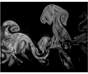
The planar Mie scattering images from four visualization experiments are shown in figure 5. The dashed white horizontal line indicates the  $y = 0$ location (i.e. geometric centreline or midway through the height of the tunnel's test section) and the solid white horizontal line with two arrow heads indicates a length scale of 20 cm for all the subfigures. The flow develops a clear asymmetry in the vertical direction due to the initially unstable upper interface and initially stable lower interface of the middle layer. Note that the mixing region grows with increasing non-dimensional time $\tau$. The rising bubbles of light fluid from the middle stream seem to grow more freely than the falling spikes of heavy fluid from the top layer as the spikes encounter the heavy fluid at the lower interface. However, there is significant erosion of the lower interface due to the momentum of falling spikes, and the heavy fluid from the bottom layer gets entrained into the developing mixing region.

Figure 5. Planar Mie scattering images from all the visualization experiments. Flow is from left to right. The dashed white horizontal line indicates  $y = 0$ location and the solid white horizontal line with two arrow heads indicate a length scale of 20 cm.
The mixing region of multilayer RTI exhibits a high degree of mixing at late times. This is seen qualitatively at the core of the mixing region, at  $\tau \sim 12.8$ and $\tau \sim 15.8$ in figure 5. This high degree of mixing for multilayer RTI could be due to a reduced influx of fresh heavy fluid coming into the mixing region, giving sufficient time for the fluid at the core of the mixing region to molecularly mix (this high degree of molecular mixing is also evaluated quantitatively later in this paper when we discuss the molecular mixing parameter and density-specific volume correlation).
3.3. Growth of the mixing region
The growth of the mixing region in an instability-driven flow is one of the most important quantities of interest. Using self-similarity analysis, Jacobs & Dalziel (Reference Jacobs and Dalziel2005) found their mixing width to exhibit the relationship  $h_3 \approx \gamma (\sqrt {\mathcal {A}_{12} g G}) t$, with $\gamma \approx 0.5$. This growth rate equation can be non-dimensionalized, normalized and rewritten as
 \begin{equation} \frac{h_3}{G} \approx \gamma \left(\sqrt{\frac{\mathcal{A}_{12} g}{G}} \right) t = \gamma \tau . \end{equation}
 In the experiments, the width of the mixing region is evaluated from the planar Mie scattering images as well as density data obtained from PLIF measurements of the three simultaneous PIV-PLIF cases. Obtaining the mixing width is generally the same for both planar Mie scattering and PLIF. For both of these diagnostics, the middle stream is seeded with fog (for planar Mie scattering) or acetone vapor which fluoresces upon ultraviolet (UV) excitation (for PLIF). The result is a greyscale image. The black regions of the image represent pure heavy fluid, and the white regions represent pure light fluid. The regions of grey represent regions where heavy and light fluid are mixed. By ensemble-averaging several of these images ( $>200$), we get an average grey image. Now assuming the intensity or concentration $C$ of pure light fluid is 1 and $C = 0$ represents pure heavy fluid, the conservation of this passive scalar concentration $C$ gives us $G = \int \overline {C(t,y)}\,{{\rm d}y}$ (where $\overline {()}$ denotes ensemble-averaging). Here, the mixing width is defined by $h_3(t) = ({1}/{C_{max}(t)}) \int \overline {C(t,y)} \, {{\rm d}y}$ where $C_{max}(t)$ denotes the maximum of the concentration distribution $\overline {C(t,y)}$. More details on the robustness of this definition can be found in Jacobs & Dalziel (Reference Jacobs and Dalziel2005).
The non-dimensionalized, normalized mixing width  $h_3 / G$ with non-dimensional time $\tau$ is plotted in figure 6 for our experimental cases as well as for low Atwood number ( $\mathcal {A}_{12} \sim 0.002$) experimental data from Jacobs & Dalziel (Reference Jacobs and Dalziel2005). The dashed black line denotes a slope corresponding to $\gamma \approx 0.5$. Our mixing width data (for both the Atwood numbers) shows good agreement with the self-similar linear growth equation (1.3) even though our Atwood numbers are significantly larger than the Atwood numbers of the experiments of Jacobs & Dalziel (Reference Jacobs and Dalziel2005) and their self-similarity analysis was done for the Boussinesq limit, i.e. ${\mathcal {A}}_{12} \rightarrow 0$. The self-similar scaling seems to hold even for moderately high Atwood numbers. Using a least square linear fit to the mixing width data, the value of $\gamma$ from current experiments is estimated to be $\gamma = 0.41 \pm 0.01$, which is slightly lower than the value of $\gamma$ reported by Jacobs & Dalziel (Reference Jacobs and Dalziel2005).

Figure 6. Non-dimensionalized, normalized mixing width  $h_3 / G$ with non-dimensional time $\tau$ for our experimental cases ( $\mathcal {A}_{12} \sim 0.3$ and $\mathcal {A}_{12} \sim 0.6$) and for experimental data from Jacobs & Dalziel (Reference Jacobs and Dalziel2005). The dashed black fiducial represents $\gamma = 0.5$ (adapted from figure 11 of Jacobs & Dalziel (Reference Jacobs and Dalziel2005)).
3.4. Velocity measurements
One of the main advantages that convective type, statistically stationary experiments provide is the easy implementation of diagnostics for velocity measurements, like hotwire anemometry and PIV. Even though these diagnostics can be used for box-type, transient experiments, these transient experiments have to be repeated a great number of times to generate data of statistical importance.
In addition to the fact that these multilayer RTI experiments are conducted with gases and at high Atwood numbers, another major difference between these experiments and the experiments of Jacobs & Dalziel (Reference Jacobs and Dalziel2005) are velocity measurements made in the present experiments, where the present work considers the fluctuations in velocity relative to the mean bulk velocity. We plot the root mean square (r.m.s.) of streamwise (horizontal) and cross-stream (vertical) velocity fluctuations,  $u^{\prime }_{rms} = \sqrt {(\overline {{u'}^2})}$ and $v^{\prime }_{rms} = \sqrt {(\overline {{v'}^2})}$, respectively, in figure 7. We see that $v^{\prime }_{rms}$ values are slightly greater than $u^{\prime }_{rms}$ as is usually expected for buoyancy-affected flows (Akula & Ranjan Reference Akula and Ranjan2016; Mikhaeil Reference Mikhaeil2020; Mikhaeil et al. Reference Mikhaeil, Suchandra, Ranjan and Pathikonda2021). The $v^{\prime }_{rms}$ profiles are more Gaussian-like whereas some of the $u^{\prime }_{rms}$ profiles are more flatter (plateau-like). The $v^{\prime }_{rms}$ profile for the experimental case $\mathcal {A}_{12} \sim 0.3,\ \tau \sim 17.3$ starts to show a plateau-like profile. As seen later in this section, our r.m.s. density fluctuation profiles at late times show a flatter, plateau-like profile. This observation could be linked to the density field showing inertial subrange scales earlier than velocity (de Stadler, Sarkar & Brucker Reference de Stadler, Sarkar and Brucker2010; Akula et al. Reference Akula, Suchandra, Mikhaeil and Ranjan2017).

Figure 7. Horizontal and vertical r.m.s. of velocity fluctuation profiles, (a)  $u^{\prime }_{rms}(y)$ and (b) $v^{\prime }_{rms}(y)$, respectively.
Here  $v^{\prime }_{rms}$ is of particular interest for buoyancy – or RTI-affected flows as the growth rate of the mixing region is usually of the order of vertical velocity fluctuations, i.e. $\dot {h} \sim v^{\prime }_{rms}$ (Snider & Andrews Reference Snider and Andrews1994; Akula et al. Reference Akula, Andrews and Ranjan2013; Akula & Ranjan Reference Akula and Ranjan2016; Akula et al. Reference Akula, Suchandra, Mikhaeil and Ranjan2017; Mikhaeil Reference Mikhaeil2020; Mikhaeil et al. Reference Mikhaeil, Suchandra, Ranjan and Pathikonda2021). The $v^{\prime }_{rms}$ profiles are normalized using different velocity scales of relevance, and these normalized profiles are presented in figure 8. The $y$ axis is shifted using the maximum of the $v^{\prime }_{rms}$ profile and normalized using the mixing width $h_3$. The first velocity scale tested, $v_s \sim \dot {h}_3 \approx \gamma \sqrt {\mathcal {A}_{12} gG}$, is obtained by taking the time derivative of the self-similar three-layer growth equation (1.3). Note that this velocity scale is independent of time. As seen in figure 8(a), $v_s \sim \gamma \sqrt {\mathcal {A}_{12} g G}$ brings the peaks of $v^{\prime }_{rms}$ closer, but the profiles are quite distinguishable. Next, we try a velocity scale $v_s \sim \mathcal {A}_{12} \sqrt {g G}$ which is independent of time but has a stronger dependence on Atwood number $\mathcal {A}_{12}$. This is shown in figure 8(b). Normalization of velocity fluctuations using this velocity scale works the best and there is a good collapse between the profiles. This suggests that for velocity alone, the self-similar linear growth equation (1.3) underpredicts the dependence of velocity fluctuations and resultant turbulence on Atwood number.

Figure 8. Vertical velocity fluctuation profiles (r.m.s. values) for two Atwood numbers,  $\mathcal {A}_{12} \sim 0.3$ and $\mathcal {A}_{12} \sim 0.6$, normalized using different velocity scales.
Next, we try two more velocity scales,  $v_s \sim 2 \alpha \mathcal {A}_{12} g t$ and $v_s \sim \sqrt {\mathcal {A}_{12} g h_3}$ as shown in figures 8(c) and 8(d), respectively. Here $v_s \sim 2 \alpha \mathcal {A}_{12} g t$ is obtained by taking the time derivative of two-layer RTI growth equation (1.2) and $v_s \sim \sqrt {\mathcal {A}_{12} g h_3}$ is used to compare results between Reynolds-averaged Navier–Stokes models and direct numerical simulations (Schwarzkopf et al. Reference Schwarzkopf, Livescu, Baltzer, Gore and Ristorcelli2016; Mikhaeil Reference Mikhaeil2020). Both these scales perform substantially worse than the first two scales. In particular, these last two scales fail to adjust the high Atwood number case at early time during instability development.
Measurements of mixing widths and velocity fluctuations enable the calculation of mixing Reynolds number  ${Re}$, Kolmogorov microscale $\eta$, and Taylor microscale $\lambda _T$ based on actual experimental values, which are reported in table 3. The values of the mixing Reynolds number calculated using measured velocity fluctuations ( ${{Re}}_{v'}$) vary considerably from the estimates of ${{Re}}_{{\dot {h}}_{3}}$ in table 1. This is due to stronger dependence of velocity fluctuations on Atwood number than that predicted by $\dot {h}_3$. The predicted and experimentally obtained values of $\eta$ and $\lambda _T$ are similar, confirming our diagnostics are capturing these spatial scales.
3.5. Density measurements
From our simultaneous PIV-PLIF experiments, in addition to velocity, we also obtain density fields for the flow. The mean density profiles,  $\bar {\rho }(y)$, for our experimental cases are shown in figure 9(a). The profiles look Gaussian-like. The shifting of the mixing centreline (where the mean density is minimum) above the geometric centreline is observed. The mean density profiles are normalized using mixture density $\rho _{mix}$ obtained assuming a completely mixed top and middle layer (Jacobs & Dalziel Reference Jacobs and Dalziel2005). If the top layer has an initial thickness $H$ and density $\rho _1$ while the middle layer has an initial thickness $G$ and density $\rho _2$, then $\rho _{mix} = (H \rho _1 + G \rho _{2})/(H + G)$. The $y$ axis is normalized in the usual way as done for velocity, by shifting the extremum and normalizing using the mixing width $h_3$. The normalized mean density profiles are shown in figure 9(b). There is a very good collapse of the density profiles, closer around the mixing centreline than the edges of the mixing region. This indicates that $\rho _{mix}$ is a good choice for the normalization factor when there is a high degree of molecular mixing at the core of the mixing region (the definition of $\rho _{mix}$ assumes complete mixing of the top and middle layers).

Figure 9. (a) Mean density profiles  $\bar {\rho }(y)$. (b) Mean density profiles normalized by $\rho _{mix}$.
Next, we present r.m.s. density fluctuations ( ${\rho }^{\prime }_{rms}$) in figure 10. From figure 10, we observe that with increasing time, the shape of the density fluctuation goes from a somewhat Gaussian-like to a more flat and plateau-like shape, indicating development of a more homogeneous core of the mixing region with time. At very late time, the peak of the ${\rho }^{\prime }_{rms}$ profile is almost flat but significantly lower in magnitude. The peaks of dimensional $\bar {\rho }(y)$ and ${\rho }^{\prime }_{rms}$ are at close $y$ locations and they also correspond very closely with the peaks of dimensional $v^{\prime }_{rms}$ (from figure 7b).

Figure 10. Density fluctuations  ${\rho }^{\prime }_{rms}$ profiles.
3.6. Measures of molecular mixing
So far, we have mostly looked at molecular mixing from a qualitative point of view. In this subsection, we look at quantifying the degree of molecular mixing in multilayer RTI flows.
3.6.1. Density-specific volume correlation
The density-specific volume correlation  $b = -\overline {\rho ^{\prime } ({1}/{\rho })^{\prime }}$ is an important dimensionless parameter used in variable density turbulence (VDT) models (Besnard, Harlow & Rauenzahn Reference Besnard, Harlow and Rauenzahn1987; Besnard et al. Reference Besnard, Harlow, Rauenzahn and Zemach1992). Here $b$ is a measure of potential for future mixing and varies from 0, representing a perfect mixture, to $b_{max} = {\bar {f}}_{1} {\bar {f}}_{2} ({{(\rho _1 - \rho _2)}^2}/{\rho _1 \rho _2})$, representing completely unmixed fluids (Mikhaeil Reference Mikhaeil2020). Here $f_i$ indicates the volume fraction of the $i$th fluid and $\overline {f_1} = 1 - \overline {f_2}$. We get $\overline {f_1}$ from the light middle layer fluid concentration distribution $\bar {C}$ discussed previously.
We present profiles of  $b$ normalized by $b_{max}$, in figure 11(a). A very low value of $b/b_{max}$ is seen for the multilayer RTI flows, approximately an order of magnitude lower than that typically observed for two-layer RTI flows ( $b/b_{max} \sim 0.3$ at late times in two-layer RTI experiments of Mikhaeil (Reference Mikhaeil2020) and Mikhaeil et al. (Reference Mikhaeil, Suchandra, Ranjan and Pathikonda2021)). For the $\mathcal {A}_{12} \sim 0.3,\ \tau \sim 11.1$ case, we see multiple peaks in the $b/b_{max}$ profile indicating greater potential for further mixing near the edges of the mixing region. Note the relatively flat profiles of $b/b_{max}$ at late times indicating that the potential for mixing is low and nearly constant through the mixing region, rather than peaking at the mixing centreline.

Figure 11. Profiles of (a) normalized density-specific volume correlation  $b/b_{max}$, and (b) molecular mixing parameter $\theta$ ( $y$ axis normalized).
3.6.2. Molecular mixing parameter
The degree of desegregation of materials in a mixture is quantified using the molecular mixing parameter  $\theta$ (Danckwerts Reference Danckwerts1952) which is defined by the following set of equations:
 $$\begin{gather} \theta = 1 - \frac{B_0}{B_2}, \end{gather}$$
 $$\begin{gather}B_0 = \lim_{T\to\infty} \frac{1}{T} \int_{0}^{\rm T} \frac{(\rho - \bar{\rho})^2}{(\Delta \rho)^2} {\rm d} t, \end{gather}$$
 $$\begin{gather}B_2 = \overline{f_{1}}\, \overline{f_{2}}. \end{gather}$$
 The averaging in time is equivalent to the ensemble-averaging we have done for other quantities, because of the statistically stationary nature of gas tunnel experiments. Here  $\theta$ varies between zero and unity, with $\theta = 0$ representing unmixed fluids and $\theta = 1$ representing fluids completely molecularly mixed. For two-layer RTI experiments, it has been reported that $\theta \rightarrow 0.75$ in the self-similar turbulent regime (Youngs Reference Youngs1991; Linden, Redondo & Youngs Reference Linden, Redondo and Youngs1994; Ramaprabhu & Andrews Reference Ramaprabhu and Andrews2004; Banerjee et al. Reference Banerjee, Kraft and Andrews2010; Akula & Ranjan Reference Akula and Ranjan2016; Mohaghar et al. Reference Mohaghar, Carter, Musci, Reilly, McFarland and Ranjan2017, Reference Mohaghar, Carter, Pathikonda and Ranjan2019).
Profiles of  $\theta$ are presented in figure 11(b), with the $y$ axis normalized. Clearly, the $\theta$ profiles are very closely related to the $b/b_{max}$ profiles, such that $\theta \sim (1 - b/b_{max})$. We see very high values of $\theta$, almost approaching unity at late times. Again, as with normalized density-specific volume correlation, the mixing seems to be quite uniform in the core of the mixing region. Such a high degree of mixing is expected when the entrainment rate (pure fluid moving into the mixing region) is slowed at late times (Orlicz, Balasubramanian & Prestridge Reference Orlicz, Balasubramanian and Prestridge2013).
3.7. Simultaneous velocity–density measurements
Implementation of simultaneous PIV-PLIF diagnostics for our multilayer RTI-affected flows allows calculation of velocity–density cross-statistics as well as conditional statistics (Akula & Ranjan Reference Akula and Ranjan2016; Mikhaeil Reference Mikhaeil2020; Mikhaeil et al. Reference Mikhaeil, Suchandra, Ranjan and Pathikonda2021). These are discussed in detail in this subsection.
3.7.1. Vertical turbulent mass flux
Vertical turbulent mass flux  $a_y$, defined as
 \begin{equation} a_y = \frac{\overline{\rho^{\prime} {v}^{\prime}}}{\bar{\rho}}, \end{equation}
is a dominant term driving the turbulent development of buoyancy-affected flows and it is one of the important quantities modelled with a transport equation in VDT models like the BHR (Besnard–Harlow–Rauenzahn) models (Besnard et al. Reference Besnard, Harlow and Rauenzahn1987, Reference Besnard, Harlow, Rauenzahn and Zemach1992; Schwarzkopf et al. Reference Schwarzkopf, Livescu, Gore, Rauenzahn and Ristorcelli2011, Reference Schwarzkopf, Livescu, Baltzer, Gore and Ristorcelli2016; Denissen et al. Reference Denissen, Fung, Reisner and Andrews2012). As per the definition used in (3.5),  $a_y$ has dimensions of velocity (length/time). In buoyancy-affected flows, as light fluid parcels (associated with $\rho ^{\prime } < 0$) usually move upward (upward movement associated with $v^{\prime } > 0$) and heavy fluid parcels (associated with $\rho ^{\prime } > 0$) usually move downward (downward movement associated with $v^{\prime } < 0$), $\overline {\rho ^{\prime } {v}^{\prime }}$ and $a_y$ predominantly have negative values for buoyancy-affected flows like RTI-affected flows.
The profiles of vertical turbulent mass flux  $a_y$ from our experiments are shown in figure 12. The peak negative values of $a_y$ in the upper domain of the flow ( $y > 0$) are close to the values of $a_y$ obtained for two-layer RTI experiments by Mikhaeil (Reference Mikhaeil2020) and Mikhaeil et al. (Reference Mikhaeil, Suchandra, Ranjan and Pathikonda2021) done at $\mathcal {A} \sim 0.1$. The profiles of $a_y$ in this upper domain are Gaussian-like but at very late time ( $\tau \sim 17.3$ case), the magnitude of $a_y$ is significantly lower and the profile looks flatter, plateau-like as observed at late time for two-layer RTI as well (Mikhaeil Reference Mikhaeil2020).

Figure 12. Profiles of vertical turbulent mass flux  $a_y$, obtained from simultaneous PIV-PLIF experiments.
An interesting feature to note in the profiles of  $a_y$ in figure 12 are the positive values of $a_y$ observed in the lower domain ( $y < 0$) around the lower edge of the mixing region. This is due to the entrainment and erosion at the lower edge of the mixing region, leading to the heavy bottom layer fluid (which would be associated with $\rho ^{\prime } > 0$) moving upward (upward movement associated with $v^{\prime } > 0$) into the mixing region, thus leading to positive values of $\overline {\rho ^{\prime } {v}^{\prime }}$ and $a_y$. This observation has a great significance for VDT modelling where profiles for statistics like $a_y$ are usually assumed Gaussian or quadratic. Oscillatory/sinusoidal profiles for statistics should be considered when modelling variable density turbulent flows in a multilayer environment.
Next, we look at scaling  $a_y$ profiles in figure 13, as was done previously for $v^{\prime }_{rms}$ in figure 8. The four velocity scales tested, as with $v^{\prime }_{rms}$, are (a) $v_s \sim \dot {h}_3 \approx \gamma \sqrt {\mathcal {A}_{12} gG}$, (b) $v_s \sim \mathcal {A}_{12} \sqrt {g G}$, (c) $v_s \sim 2 \alpha \mathcal {A}_{12} g t$ and (d) $v_s \sim \sqrt {\mathcal {A}_{12} g h_3}$. This time, the velocity scale $v_s \sim \dot {h}_3 = \gamma \sqrt {\mathcal {A}_{12} gG}$ seems to work the best in normalizing negative peaks of $a_y$ (in the upper domain, $y > 0$, where the flow is mostly buoyancy-affected), followed by the velocity scale $v_s \sim \sqrt {\mathcal {A}_{12} g h_3}$. This suggests that the dependence of the vertical turbulent mass flux on the Atwood number is adequately predicted by the self-similar three-layer growth rate. In other words, $\dot {h}_3 \sim |a_y|$ is a better scaling than $\dot {h}_3 \sim v^{\prime }_{rms}$ for three-layer flows as suggested by the experimental data. Note that none of the four velocity scales seem to work at very late time, for $\tau \sim 17.3$ case, possibly due to breaking of self-similarity as the entrainment rate is significantly slowed at late times (Orlicz et al. Reference Orlicz, Balasubramanian and Prestridge2013). Also at very late time, as the upper edge of the mixing region approaches the upper wall of the test section, deviation from self-similarity could be expected as observed by Jacobs & Dalziel (Reference Jacobs and Dalziel2005) in their experiments.

Figure 13. Profiles of vertical turbulent mass flux  $a_y$, normalized using different velocity scales.
3.7.2. Conditional turbulence statistics
Simultaneous measurements of velocity and density allow us to look at fluctuation quantities or turbulence statistics of the flow under specified conditions. Conditional statistics can be used to separate the relative importance of bubble and spike structures (or parcels of light or heavy fluids) on fluctuation quantities. These statistics serve as valuable inputs for setting model constants in VDT models, as shown by Adrian (Reference Adrian1975). Following the methods of Banerjee et al. (Reference Banerjee, Kraft and Andrews2010), Akula & Ranjan (Reference Akula and Ranjan2016) and Mikhaeil (Reference Mikhaeil2020), we present total and conditional statistics in this subsection under four sampling conditions: (a)  $\rho ^{\prime } > 0$, (b) $\rho ^{\prime } < 0$, (c) $v^{\prime } > 0$ and (d) $v^{\prime } < 0$. These statistics are evaluated at the core of the mixing region (region around the mixing centreline). The statistics are studied via the p.d.f. The p.d.f. of a continuous random variable (like velocity or density fluctuations in a turbulent flow) describes the likelihood of the variable to be around a particular value (Papoulis & Pillai Reference Papoulis and Pillai2002; Bendat & Piersol Reference Bendat and Piersol2010; Davidson Reference Davidson2015).
Figures 14, 15 and 16 show p.d.f. of  $v^{\prime }$, $\rho ^{\prime }$ and $\rho ^{\prime } {v}^{\prime }$ under the sampling conditions discussed previously. Many expected general trends of buoyancy-affected flows are seen. Due to the mostly negative correlation between velocity and density fluctuations in buoyancy-affected flows, the p.d.f. ( $v^{\prime }$) sampled under the condition of $\rho ^{\prime } > 0$ has more area on the negative side (higher probability of $v^{\prime }$ being negative) and the p.d.f. ( $v^{\prime }$) sampled under the condition of $\rho ^{\prime } < 0$ has more area on the positive side. Similarly, the p.d.f. ( $\rho ^{\prime }$) sampled under the condition of $v^{\prime } > 0$ has more area on the negative side and the p.d.f. ( $\rho ^{\prime }$) sampled under the condition of $v^{\prime } < 0$ has more area on the positive side. The total p.d.f. ( $v^{\prime }$) and p.d.f. ( $\rho ^{\prime }$) are not always necessarily symmetric nor Gaussian-like, owing to asymmetric development of the flow in the vertical direction. This was also observed at moderately high Atwood number in two-layer RTI experiments of Akula & Ranjan (Reference Akula and Ranjan2016) as RTI spikes and bubbles develop asymmetrically at large density differences. The p.d.f. ( $\rho ^{\prime } {v}^{\prime }$) has sharp peaks, long negative tails and usually more area on the negative side (higher probability of $\rho ^{\prime } {v}^{\prime }$ being negative), as generally expected in buoyancy-driven flows (Banerjee et al. Reference Banerjee, Kraft and Andrews2010; Akula & Ranjan Reference Akula and Ranjan2016; Akula et al. Reference Akula, Suchandra, Mikhaeil and Ranjan2017; Mikhaeil Reference Mikhaeil2020). However, the asymmetry of p.d.f. ( $\rho ^{\prime } {v}^{\prime }$) is much less prominent than that observed for two-layer RTI. This could be due to substantial positive vertical turbulent mass flux $a_y$ associated with entrainment and erosion at the lower edge of the mixing region whose effects are felt at the mixing core as well.

Figure 14. The p.d.f. of different turbulence statistics, total and conditional, evaluated at the mixing core for the experimental case of  $\mathcal {A}_{12} \sim 0.3,\ \tau \sim 11.1$.

Figure 15. The p.d.f. of different turbulence statistics, total and conditional, evaluated at the mixing core for the experimental case of  $\mathcal {A}_{12} \sim 0.6,\ \tau \sim 15.1$.

Figure 16. The p.d.f. of different turbulence statistics, total and conditional, evaluated at the mixing core for the experimental case of  $\mathcal {A}_{12} \sim 0.3,\ \tau \sim 17.3$.
A summary of different turbulence statistics evaluated at the mixing core under different sampling conditions for our experimental cases is presented in tables 4, 5 and 6. Again, some general expected trends of buoyancy-affected flows are observed. For example, positive  $\overline {v^{\prime }}$ is associated with the condition of $\rho ^{\prime } < 0$ and vice versa. Similarly, positive $\overline {\rho ^{\prime }}$ is associated with the condition of $v^{\prime } < 0$ and vice versa. Note that there are small but noticeable asymmetries between the conditional statistics from opposite sampling conditions, unlike those observed in two-layer RTI experiments at low Atwood numbers by Mikhaeil (Reference Mikhaeil2020) and Mikhaeil et al. (Reference Mikhaeil, Suchandra, Ranjan and Pathikonda2021). Asymmetries in conditional statistics from our experiments resemble asymmetries in conditional statistics from the two-layer RTI experiments at moderately high Atwood numbers (Akula & Ranjan Reference Akula and Ranjan2016), owing to asymmetric flow evolution in the vertical direction.
Table 4. Conditional statistics evaluated at the mixing core from the simultaneous PIV-PLIF experiment at  $\mathcal {A}_{12} \sim 0.3,\ \tau \sim 11.1$ (all values are in SI units).

Table 5. Conditional statistics evaluated at the mixing core from the simultaneous PIV-PLIF experiment at  $\mathcal {A}_{12} \sim 0.6,\ \tau \sim 15.1$ (all values are in SI units).

Table 6. Conditional statistics evaluated at the mixing core from the simultaneous PIV-PLIF experiment at  $\mathcal {A}_{12} \sim 0.3,\ \tau \sim 17.3$ (all values are in SI units).

3.8. Energetics of multilayer RTI
Apart from calculations of velocity–density cross-statistics and conditional statistics, simultaneous velocity–density measurements also make it possible to analyse energy transfer and distribution in variable density turbulent flows, as calculations related to energetics require information about both the density field (mostly in order to calculate potential energy in the flow) as well as information about the velocity field (mostly to calculate kinetic energy). In this subsection, we look at the distribution of local, ensemble-averaged turbulent kinetic energy (denoted by  $k$) as well as integrated measures of energetics like bulk changes in potential and kinetic energy release, and mixing efficiency $\eta _{mix}$.
3.8.1. Turbulent kinetic energy
The local, time- or ensemble-averaged turbulent kinetic energy  $k = \frac {1}{2} \bar {\rho } <{(u^{\prime }_{rms})}^2 + {(v^{\prime }_{rms})}^2 + {(w^{\prime }_{rms})}^2>$ (Akula Reference Akula2014; Akula & Ranjan Reference Akula and Ranjan2016) is an indicator of how much energy of the flow is due to velocity fluctuations rather than due to mean velocity. Calculation of $k$ requires all three velocity components. Due to the absence of spanwise velocity measurements, we make the assumption $u^{\prime } \sim w^{\prime }$ (Mikhaeil Reference Mikhaeil2020; Mikhaeil et al. Reference Mikhaeil, Suchandra, Ranjan and Pathikonda2021) as the streamwise and spanwise directions are not in the direction of the pressure gradient due to gravity. Therefore, the streamwise and spanwise directions are the homogeneous directions in an inertial reference frame moving with the mean convective speed of the flow. As we do not have complete profiles of r.m.s. velocity fluctuations or mean density through the complete vertical extent of the gas tunnel, Gaussian fits are used with our data, following the methodology of Akula & Ranjan (Reference Akula and Ranjan2016), to obtain $k$ profiles.
The profiles of  $k$ from our simultaneous PIV-PLIF experiments are presented in figure 17. The dependence of velocity fluctuations and thus $k$ on Atwood number can be seen. Also, at very late time, the $k$ production is diminished. This is shown in the next subsection as well.

Figure 17. Profiles of turbulent kinetic energy  $k$, for different experimental conditions.
3.8.2. Potential energy release
In stratified flows, like RTI, the gravitational potential energy stored in density stratification is released and converted into either turbulent kinetic energy (assuming the kinetic energy of the mean flow stays the same), or gets dissipated due to viscous effects. At a streamwise location  $x$, the potential energy per unit width $PE(x)$, in a statistically stationary sense, is calculated by integrating the mean density profile across the entire vertical extent $y$ of the flow domain at that streamwise location. This is given by
 \begin{equation} PE(x) = \int \bar{\rho} g y \, {{\rm d}y}. \end{equation}
 In a similar fashion, the integrated total turbulent kinetic energy per unit width  $KE(x)$ at a streamwise location $x$ is calculated by integrating the $k$ profile across the vertical extent of the flow, as given by
 \begin{equation} KE(x) = \int k \, {{\rm d}y}. \end{equation}
 By assuming a step change in density at  $x = 0$, $PE(x=0) = PE_0$ is calculated. For $KE(x=0)$, we use the value of $k$ outside the mixing region, specifically from the region below the mixing region. This gives us $KE(x=0) = KE_0$. Thus, for our experimental cases, the potential energy released is given by $\Delta PE(x) = PE_0 - PE(x)$ and the increase in total, integrated turbulent kinetic energy is given by $\Delta KE(x) = KE(x) - KE_0$. The dissipated energy is calculated as the remainder of the potential energy, $D(x) = \Delta PE(x) - \Delta KE(x)$.
The ratio of total turbulent kinetic energy generated by multilayer RTI and dissipated energy to the potential energy released,  $\Delta KE / \Delta PE$ and $D / \Delta PE$, are plotted in figure 18. We observe very low values of $\Delta KE / \Delta PE$ for our flows, approximately 0.2–0.25, which is approximately half the magnitude of $\Delta KE / \Delta PE$ observed for typical two-layer RTI flows ( $\Delta KE / \Delta PE \sim 0.5$ for two-layer RTI flows (Youngs Reference Youngs1991; Linden et al. Reference Linden, Redondo and Youngs1994; Ramaprabhu & Andrews Reference Ramaprabhu and Andrews2004; Banerjee et al. Reference Banerjee, Kraft and Andrews2010; Akula Reference Akula2014; Akula & Ranjan Reference Akula and Ranjan2016; Mikhaeil Reference Mikhaeil2020; Mikhaeil et al. Reference Mikhaeil, Suchandra, Ranjan and Pathikonda2021)). A possible explanation could be as follows: at late times, as mentioned previously when discussing molecular mixing, the multilayer RTI shows a high degree of molecular mixing and reduced turbulent mass fluxes. Thus, there is not enough $k$ production at late times and most of the energy gets dissipated by viscous effects leading to high values of $D / \Delta PE$.

Figure 18. The ratio of total turbulent kinetic energy generated by multilayer RTI,  $\Delta KE$ and dissipated energy, $D$, to the potential energy released, $\Delta PE$, at different times in the instability development. Note that $\Delta KE / \Delta PE + D / \Delta PE = 1$. The vertical error bars are due to least squared error of the Gaussian-fits used to obtain $k$ profiles and the horizontal error bars are due to uncertainty in $\tau$ arising due to uncertainty in $U_c$ and $\mathcal {A}_{12}$.
Next, we look at mixing efficiency for our multilayer RTI flows, a quantity which is closely related to the potential energy release.
3.8.3. Mixing efficiency
Mixing efficiency  $\eta _{mix}$ is an important quantity used to describe the extent of overall molecular mixing and is often used by researchers in the atmospheric and oceanic science communities (Fernando Reference Fernando1991; Holford & Linden Reference Holford and Linden1999; Tseng & Ferziger Reference Tseng and Ferziger2001; Dalziel et al. Reference Dalziel, Patterson, Caulfield and Coomaraswamy2008; Lawrie & Dalziel Reference Lawrie and Dalziel2011; Wykes & Dalziel Reference Wykes and Dalziel2014; Wykes, Hughes & Dalziel Reference Wykes, Hughes and Dalziel2015; Williams Reference Williams2017). Mixing efficiency is the ratio of the energy used by (or lost to) mixing, to the energy provided to the system. In order to define the mixing efficiency, a few definitions need to be considered first. Gravitational potential energy is given by $PE$ as defined previously. Now, if every fluid parcel were allowed to move adiabatically and without mixing until in stable equilibrium, the system gets rearranged to a state of minimum potential energy (Lorenz Reference Lorenz1954). This is a reference state (Tailleux Reference Tailleux2013) and can be presented as a background potential energy $BE = \int \hat {\rho } g y \, {{\rm d}y}$ where $\hat {\rho }$ is the rearranged density profile obtained by simply sorting $\bar {\rho }$ such that ${\rm d}\hat {\rho }/{{\rm d}y} \leq 0$ everywhere (Peltier & Caulfield Reference Peltier and Caulfield2003). Thus, the available potential energy is defined as $AE = PE - BE$. Here $KE$ is the kinetic energy as defined in the previous subsection. Mixing efficiency of the mixing process is, therefore, defined as
 \begin{equation} \eta_{mix} = \frac{|\Delta BE|}{|\Delta (AE + KE)|} , \end{equation}
where  $\Delta$ represents the change in state of the system during the mixing process. For classic RTI experiments with two homogeneous miscible fluids in a box-type set-up, $\eta _{mix} \rightarrow 1/2$, given quiescent initial and final states (Dalziel et al. Reference Dalziel, Patterson, Caulfield and Coomaraswamy2008; Lawrie & Dalziel Reference Lawrie and Dalziel2011; Wykes & Dalziel Reference Wykes and Dalziel2014).
Mixing efficiency for the simultaneous PIV-PLIF experiments are plotted in figure 19. We observe high values of  $\eta _{mix}$ in the experiments, $\eta _{mix} \sim 0.6$. This result is in accordance with the observance of a high degree of mixing in the multilayer RTI flows. The $\eta _{mix}$ values are greater than the limiting value of $\eta _{mix} \rightarrow 0.5$ for two-layer RTI. A possible explanation for this could be as follows: in the idealized, limiting case, when there is complete mixing between the top and middle layers and the bottom layer remains undisturbed, the total mixing efficiency (mixing efficiency considering all three fluid layers of multilayer RTI configuration) is still 0.5. Now consider another theoretical case when there is mixing only between the middle and bottom layers because of entrainment and erosion. Jacobs & Dalziel (Reference Jacobs and Dalziel2005) predicts the mixing efficiency for this lower interface to be $\sim$5 % because of similarity between their mixing related results with mixing-box experiments and grid-generated turbulence studies (Fernando Reference Fernando1991; Holford & Linden Reference Holford and Linden1999). Thus, for the real case when there is mixing due to both RTI at the upper interface of the middle layer and entrainment-erosion at its lower interface, we can expect the mixing efficiency to be around $\sim$ 55 % which is the case for current measurements.

Figure 19. Mixing efficiency at different times in the instability development. The vertical error bars are due to least squared error of the Gaussian-fits used to obtain  $k$ profiles and the horizontal error bars are due to uncertainty in $\tau$ arising due to uncertainty in $U_c$ and $\mathcal {A}_{12}$.
4. Conclusions
This paper presents studies of the multilayer buoyancy-driven RTI outside the Boussinesq limit, where a thin light fluid layer is surrounded by heavier fluid layers from top and bottom. A new blow-down three-layer gas tunnel facility was built to perform multilayer RTI experiments. Experiments are performed at two Atwood numbers,  $\mathcal {A}_{12} \sim 0.3$ and $\mathcal {A}_{12} \sim 0.6$, and measurements are conducted at two streamwise locations along the tunnel. Three types of diagnostics – planar Mie scattering visualization, PIV and PLIF – are employed to obtain the mixing widths, velocity field and simultaneous velocity–density field. The key results from this work are as follows.
(i) Qualitative planar Mie scattering images show significant entrainment and erosion of the lower otherwise stable interface of the middle light fluid layer. At late times, a high degree of mixing is observed at the mixing core, due to a reduced influx of pure fluid coming into the mixing region.
(ii) The growth of the mixing region is found to be linear in time at intermediate and late times (
$\tau > 5$), similar to the self-similar late time linear growth equation for $\mathcal {A}_{12} \rightarrow 0$. The experimental data is in good agreement with the very low Atwood number experimental data of Jacobs & Dalziel (Reference Jacobs and Dalziel2005); however, a lower value of the growth equation constant $\gamma$ is estimated: $\gamma \approx 0.41$ in the current experiments and $\gamma \approx 0.5$ for Jacobs & Dalziel (Reference Jacobs and Dalziel2005). Our experiments extend and validate the self-similar three-layer mixing width growth prediction to moderately high Atwood numbers.(iii) An attempt is made to normalize velocity fluctuations so that the functional dependence of quantities like velocity fluctuations on different parameters for an experimental case can be predicted, which can later be used to come up with growth models for multilayer RTI-affected flows. It is seen qualitatively that
$v_s \sim \mathcal {A}_{12} \sqrt {g G}$ works the best in normalizing velocity fluctuations, suggesting stronger dependence of velocity fluctuations on Atwood number than that predicted from self-similar three-layer mixing width growth rate.(iv) Various quantitative measures of molecular mixing are presented, like the density-specific volume correlation and molecular mixing parameter, which all support the observation of a very high degree of molecular mixing at late times in the multilayer RTI flows.
(v) The vertical turbulent mass flux
$a_y$ is calculated in our flow which requires the simultaneous measurement of velocity and density. In addition to usual, mostly negative values of $a_y$ found in buoyancy-dominated flows due to negative correlation between velocity and density fluctuations, positive regions in the profiles of $a_y$ are observed due to entrainment and erosion at the lower edge of the mixing region. Normalization of $a_y$ suggests that $\dot {h}_3 \sim |a_y|$ is a better scaling than $\dot {h}_3 \sim v^{\prime }_{rms}$ for multilayer RTI.(vi) Conditional turbulence statistics are presented for the first time for this kind of flow, which usually serve as valuable inputs for setting model constants in VDT models.
(vii) Finally, global energy budgets are calculated for our multilayer RTI flows at late times and it is found that the majority of potential energy released has been dissipated due to viscous effects, and a large fraction of energy provided to the system has been used up in mixing (mixing efficiency
$\sim$60 %).


These experiments find their relevance in ICF studies, as shown in the following flow chart, as well as in atmospheric and oceanic fluid mechanics:
 \begin{align*} \begin{array}{@{}c@{}}
\textrm{Experimental data of statistical importance} \\
\downarrow \\
\textrm{Turbulence modelling} \\
\downarrow \\
\textrm{Multiphysics hydrocodes} \\
\downarrow \\
\textrm{ICF simulations} \\
\downarrow \\
\textrm{ICF experiments}.\end{array} \end{align*}
\begin{align*} \begin{array}{@{}c@{}}
\textrm{Experimental data of statistical importance} \\
\downarrow \\
\textrm{Turbulence modelling} \\
\downarrow \\
\textrm{Multiphysics hydrocodes} \\
\downarrow \\
\textrm{ICF simulations} \\
\downarrow \\
\textrm{ICF experiments}.\end{array} \end{align*}
These experimental data are also useful for developing and validating VDT models. For example, the profiles of density-specific volume correlation and vertical turbulent mass flux presented here can be used to develop evolution equations for VDT models, like those shown in Schwarzkopf et al. (Reference Schwarzkopf, Livescu, Baltzer, Gore and Ristorcelli2016). Additionally, the data presented here can help develop growth models, similar to Davies & Taylor (Reference Davies and Taylor1950), Layzer (Reference Layzer1955) and Goncharov (Reference Goncharov2002), for multilayer RTI outside the regime of very low density contrast.
Funding
This work was supported by the US DOE-NNSA SSAA grant no. DE-NA-0003912 and DE-NA0004099.
Declaration of interests
The authors report no conflict of interest.


 Open access