


1. Introduction
Turbulent multiphase flows are common in natural and industrial applications. Examples include aeolian sand storms (Zheng Reference Zheng2009; Pähtz et al. Reference Pähtz, Valyrakis, Zhao and Li2018; Wang et al. Reference Wang, Feng, Zheng and Sung2019; Zheng, Jin & Wang Reference Zheng, Jin and Wang2020; Jin, Wang & Zheng Reference Jin, Wang and Zheng2021; Zheng, Feng & Wang Reference Zheng, Feng and Wang2021), river sediment transport (Ancey et al. Reference Ancey, Davison, Böhm, Jodeau and Frey2008; Seminara Reference Seminara2010; Schmeeckle Reference Schmeeckle2014; Berzi, Jenkins & Valance Reference Berzi, Jenkins and Valance2016; Pähtz et al. Reference Pähtz, Clark, Valyrakis and Durán2020) and fluidized beds (Fortes, Joseph & Lundgren Reference Fortes, Joseph and Lundgren1987; Grbavcic et al. Reference Grbavcic, Garic, Hadzismajlovic, Jovanovic, Vukovic, Littman and Morgan1991; Deen et al. Reference Deen, Van Sint Annaland, Van der Hoef and Kuipers2007; Luo et al. Reference Luo, Tan, Wang and Fan2016; Esteghamatian et al. Reference Esteghamatian, Euzenat, Hammouti, Lance and Wachs2018), to name a few. In the framework of Euler–Lagrange simulations of particle-laden flows (Li et al. Reference Li, McLaughlin, Kontomaris and Portela2001; Dritselis & Vlachos Reference Dritselis and Vlachos2008; Eaton Reference Eaton2009; Zhao, Andersson & Gillissen Reference Zhao, Andersson and Gillissen2010, Reference Zhao, Andersson and Gillissen2013; Capecelatro & Desjardins Reference Capecelatro and Desjardins2013; Schmeeckle Reference Schmeeckle2014; Guan et al. Reference Guan, Salinas, Zgheib and Balachandar2021; Zheng et al. Reference Zheng, Feng and Wang2021), the quasi-steady drag force is perhaps the most dominant of all the hydrodynamic force contributions (Guan et al. Reference Guan, Salinas, Zgheib and Balachandar2021). The coupling between the particle and fluid also needs to be realized by adding integral or distributed drag force feedback, among others, into the momentum equation (Rouson Reference Rouson1997; Li et al. Reference Li, McLaughlin, Kontomaris and Portela2001; Rouson & Eaton Reference Rouson and Eaton2001; Beetstra, van der Hoef & Kuipers Reference Beetstra, van der Hoef and Kuipers2007; Dritselis & Vlachos Reference Dritselis and Vlachos2008; Eaton Reference Eaton2009; Zhao et al. Reference Zhao, Andersson and Gillissen2013). Even in the Eulerian–Eulerian approach, the coupling terms by averaged equations for momentum also need to be modelled by drag force (Tenneti, Garg & Subramaniam Reference Tenneti, Garg and Subramaniam2011; Chen et al. Reference Chen, Song, Jiang, Ma and Zhou2020). Therefore, the drag model is vital for the accuracy of simulations and is one of the key issues of turbulent multiphase flow (Balachandar & Eaton Reference Balachandar and Eaton2010). Unfortunately, although many drag models have been proposed under relatively ideal conditions, their applicability for actual turbulent multiphase flow has not been well established so far.
Stokes (Reference Stokes1851) first proposed the well-known Stokes drag force  $\boldsymbol {F}_D=3{\rm \pi} \mu D_p\boldsymbol {U}_{\infty }$ for a single isolated sphere subject to a steady uniform Stokes flow, where $\boldsymbol {F}_D$ is the drag force, $D_p$ and $\mu$ are the particle diameter and dynamic viscosity of the fluid, respectively, and $\boldsymbol {U}_{\infty }$ is the free-stream velocity usually being used as the particle–fluid slip velocity $\boldsymbol {u}_{slip}$ in practice. This drag model is valid in the limit of ${Re_p}\rightarrow 0$, with the particle Reynolds number ${Re}_p$ being defined as $\boldsymbol {u}_{slip}D_p/\nu$, where $\nu$ is the kinematic viscosity of the fluid. When the deviation from Stokes flow or the presence of neighbouring particles is considered, the Stokes drag model has to be modified. The correction to the Stokes drag force for ${Re_p}> 0$ was completed theoretically by Oseen (Reference Oseen1910) who proposed a first-order slip-based inertial correction. However, most of the drag correction schemes through theoretical analysis are still limited to ${Re_p}\rightarrow 0$ in either unbounded models (Hasimoto Reference Hasimoto1959; Batchelor Reference Batchelor1972; Proudman & Pearson Reference Proudman and Pearson1957; Sangani & Acrivos Reference Sangani and Acrivos1982) or bounded models, including the effect of walls on drag force (Faxén Reference Faxén1922; Vasseur & Cox Reference Vasseur and Cox1977; Happel & Brenner Reference Happel and Brenner1981). Works on a purely theoretical basis are rather difficult for systems in which the volume fraction $\phi _p$ and particle Reynolds number are non-zero, or more complex influencing factors are involved. For the experiments, measurements based on a pressure drop over packed beds of various materials (Ergun Reference Ergun1952; Epstein Reference Epstein1954; Rumpf & Gupte Reference Rumpf and Gupte1971; Fand et al. Reference Fand, Kim, Lam and Phan1987; Watanabe Reference Watanabe1989) are usually used to obtain estimates for the solid particle drag when $\phi _p> 0.1$ and $Re_p > 1$. In addition, some studies also reported particle acceleration and trajectory tracking using non-intrusive measurements such as a high-speed camera, tomographic particle image velocimetry and the shake-the-box method (Ayyalasomayajula et al. Reference Ayyalasomayajula, Gylfason, Collins, Bodenschatz and Warhaft2006; Wu et al. Reference Wu, Wang, Liu, Li, Zhang and Zheng2006; Qureshi et al. Reference Qureshi, Arrieta, Baudet, Cartellier, Gagne and Bourgoin2008; Schanz, Gesemann & Schröder Reference Schanz, Gesemann and Schröder2016). However, such experiments provide only indirect information of drag force, and are often not well defined in terms of details such as homogeneity, mobility and so on (Beetstra et al. Reference Beetstra, van der Hoef and Kuipers2007). Most importantly, detailed experimental measurements of particle drag force in an actual multiphase flow, as turbulent two-phase flow over the erodible bed concerned in this paper, are rare and as a result, high-quality data are scarce. In fact, experimental observation is also a great challenge due to particle aggregation and two-phase interaction.
Different from the experimental and analytic methods, particle-resolved direct numerical simulation (PR-DNS) in the framework of body-conforming moving-mesh methods (Feng, Hu & Joseph Reference Feng, Hu and Joseph1994a,Reference Feng, Hu and Josephb; Hu, Patankar & Zhu Reference Hu, Patankar and Zhu2001) or immersed boundary methods (IBMs) (Peskin Reference Peskin1977; Uhlmann Reference Uhlmann2005; Breugem Reference Breugem2012; Luo et al. Reference Luo, Wang, Tan and Fan2019) evaluates the hydrodynamic force on a particle by integrating the pressure and viscous stresses around the particle surface. The exponential growth in computing power over the past 20 years made PR-DNS become a preferred choice for developing more accurate drag correlations over a larger range of  $\phi _p$, ${Re}_p$ (Brandt & Coletti Reference Brandt and Coletti2022) and parameter space. Zeng et al. (Reference Zeng, Najjar, Balachandar and Fischer2009) obtained the hydrodynamic force acting on a finite-sized particle translating parallel to the wall in a stagnant fluid and a stationary particle in a wall-bounded linear shear flow by PR-DNS, based on which a composite drag correlation that is valid for a wide range of $2< Re_p<250$ and distance from the wall $L$ was proposed. Lee & Balachandar (Reference Lee and Balachandar2010) furthered this study to a more general case of a translating and rotating particle in a wall-bounded linear shear flow. They provided a composite drag correlation that linearly superposes shear, translational and rotational effects. Ekanayake et al. (Reference Ekanayake, Berry, Stickland, Dunstan, Muir, Dower and Harvie2020) and Ekanayake, Berry & Harvie (Reference Ekanayake, Berry and Harvie2021) simulated finite-sized particles in both quiescent and linear shear flows with low slip and shear Reynolds numbers. A new drag coefficient correlation that includes higher-order terms in separation distance and the shear-based inertial correction was proposed and tested in a linear shear flow. For the dense flow, the effects of neighbouring particles, through displacing the local fluid, become important and must be accounted for. The fully resolved simulations have also been applied to study the drag force in flow through arrays of structured and random particles (fixed or moving). In this regard, modified drag models need to consider additional parameters, such as the solid volume fraction gradient, superficial velocity gradient (Chen et al. Reference Chen, Song, Jiang, Ma and Zhou2020), the granular temperature (Zhou & Fan Reference Zhou and Fan2014, Reference Zhou and Fan2015; Tang, Peters & Kuipers Reference Tang, Peters and Kuipers2016; Huang et al. Reference Huang, Wang, Zhou and Li2017), the particle velocity fluctuation (Luo et al. Reference Luo, Wang, Jin, Wang, Wang, Tan and Fan2021) and so on.
In the turbulent boundary layer, these drag models developed in laminar upstream flows are proven to have limited effectiveness. Zeng et al. (Reference Zeng, Balachandar, Fischer and Najjar2008) simulated isolated finite-sized particles with diameters varying from  $3.5$ to $25$ wall units ( $D_p/\eta =2.0 \sim 14.3$, where $\eta$ shows the Kolmogorov scale) and located in the buffer region and along the centreplate of channel turbulence. They found that, near the wall, only for small particles (away from the viscous sublayer) under consideration, the instantaneous force is captured well with the standard drag formulation of Schiller & Nauman (Reference Schiller and Nauman1935). Within the buffer layer, the force fluctuation can be correlated well with incoming turbulent flow structures. With increasing particle size, vortex shedding contributes to an increase in drag fluctuation that cannot be captured by the standard drag model. Homann, Bec & Grauer (Reference Homann, Bec and Grauer2013) pointed out that the average drag force increases as a function of the turbulent intensity. This increase is larger than what is predicted by standard drag correlations developed based on laminar upstream flows. Li et al. (Reference Li, Balachandar, Lee and Bai2019) investigated the forces on a stationary finite-sized particle in wall turbulence over a rough bed and the interaction between the particle and the near-wall turbulent structures. They found that the standard drag formulation with near-wall correction proposed by Zeng et al. (Reference Zeng, Najjar, Balachandar and Fischer2009) can reasonably predict the drag force, provided that the slip velocity is correctly calculated. Again, the large fluctuations due to self-induced vortex shedding probably result in a significant discrepancy. Recently in Li et al. (Reference Li, Huang, Zhao and Xu2020), a spherical particle released and suspended in a turbulent open channel flow was tracked by PR-DNS. It is found that the standard drag formulation of Schiller & Nauman (Reference Schiller and Nauman1935) can only reflect the general trend of drag, with the large-amplitude and high-frequency characteristic of the surface forces missed.
In the past two decades a number of PR-DNS investigations of finite-sized particles have also been documented for turbulent two-phase flows. Such studies focused on either turbulence modulation (Pan & Banerjee Reference Pan and Banerjee1997; Cate et al. Reference Cate, Derksen, Portela and Akker2004; Lucci, Ferrante & Elghobashi Reference Lucci, Ferrante and Elghobashi2010; Naso & Prosperetti Reference Naso and Prosperetti2010; Yeo et al. Reference Yeo, Dong, Climent and Maxey2010; Lucci, Ferrante & Elghobashi Reference Lucci, Ferrante and Elghobashi2011; Gao, Li & Wang Reference Gao, Li and Wang2013; Tanaka & Teramoto Reference Tanaka and Teramoto2015; Schneiders, Meinke & Schröder Reference Schneiders, Meinke and Schröder2017; Tanaka Reference Tanaka2017; Fornari et al. Reference Fornari, Zade, Brandt and Picano2019; Yousefi, Ardekani & Brandt Reference Yousefi, Ardekani and Brandt2020) or particle migration (Kidanemariam et al. Reference Kidanemariam, Chan-Braun, Doychev and Uhlmann2013; Kidanemariam & Uhlmann Reference Kidanemariam and Uhlmann2014; Lashgari et al. Reference Lashgari, Picano, Breugem and Brandt2016, Reference Lashgari, Picano, Costa, Breugem and Brandt2017; Kidanemariam & Uhlmann Reference Kidanemariam and Uhlmann2017; Ardekani et al. Reference Ardekani, Al Asmar, Picano and Brandt2018; Costa, Brandt & Picano Reference Costa, Brandt and Picano2020; Yousefi et al. Reference Yousefi, Ardekani, Picano and Brandt2021). The reader is referred to Brandt & Coletti (Reference Brandt and Coletti2022) for the state-of-the-art progress of particle-laden turbulence. Only a few studies, however, discussed particle forces in turbulent two-phase flows. For example, Esmaily & Horwitz (Reference Esmaily and Horwitz2018) simulated decaying turbulence laden with inertial particles using point-particle models and compared their results against a particle-resolved simulation. They revealed that the momentum exchange between particles and fluid modifies the slip velocity and produces an erroneous prediction of coupling force. A correction scheme to reduce this error and accurately predict the undisturbed fluid velocity was proposed. Costa et al. (Reference Costa, Brandt and Picano2020) simulated a one-way coupled turbulent channel flow laden with small inertial particles. A direct comparison between interface-resolved and drag-force-driven point-particle results was conducted for  $\phi _p \sim O(10^{-5})$ and $D_p^+=D_p u_{\tau,f}/\nu =3$, where $u_{\tau,f}$ is the friction velocity of particle-free wall turbulence. Ji et al. (Reference Ji, Munjiza, Avital, Ma and Williams2013) simulated sediment entrainment on an erodible particle bed in turbulent channel flow. The hydrodynamic forces acting on the particles were presented and the underlying mechanisms of sediment entrainment were discussed.
Despite the numerous studies, as summarized above, particle drag force in multiphase turbulence has not been thoroughly discussed. What are the characteristics of particle drag force in a turbulent multiphase flow and whether previously proposed drag models can predict the drag force acting on particles are still open questions, which inspire the present study. We will simulate turbulent two-phase flow over an erodible particle bed using the PR-DNS method and present an in-depth analysis of the drag force acting on saltating particles. The characteristics of this two-phase flow are: once the fluid velocity or shear velocity is high enough to exceed the threshold condition for the onset of sediment motion, the two-phase flow will come into being with particles suspending, rolling and saltating above the bed. Due to the inhomogeneous nature of wall turbulence in a wall-normal direction and the attenuation of particle concentration along the height, a saltating particle will experience varying local volume fraction, particle-wall separation distance, turbulent velocity fluctuation and mean shear during its descending and ascending phases. As a result, the factors affecting the drag force are quite complex. It is therefore of practical and physical significance to discuss the drag force on particles in such a two-phase flow. The structure of the paper is as follows. In § 2 we introduce the methodology. Dynamic responses of a typical particle during continuous saltations are presented in § 3, together with the validity check of several classical drag models. Then a new drag model is proposed by fitting the simulated results. Finally, we discuss the limits and draw conclusions in §§ 4 and 5, respectively.
2. Numerical methodology
We simulate pressure-driven open channel flow over an erodible particle bed. A Cartesian coordinate system is adopted such that  $x$,
$x$,  $y$ and $z$ denote the streamwise, wall-normal and spanwise direction, respectively. The simulation domain is $[ L_x \times L_y \times L_z ] / H=6\times 1\times 3$, where $H$ is the half-channel height. The friction Reynolds number based on $H$, the kinematic viscosity of fluid $\nu$ and particle-free friction velocity $u_{\tau,f}$ is ${Re}_{\tau,f}=u_{\tau,f}H/\nu =180$. The sediment bed consists of four layers of monodisperse spheres at rest. This quasi-randomly packed particle bed is formed by particles randomly released in the simulation domain that settle under the action of gravity (without hydrodynamic force) and collision as detailed in Kidanemariam & Uhlmann (Reference Kidanemariam and Uhlmann2014). The total number of particles is $7200$. Figure 1 shows a sketch of the computational set-up, particle bed and moving particles. The particle-to-fluid density ratio is $\rho _p/\rho _f=2.5$. The particle diameter studied is $D_p/H=0.1$ and the particle volume fraction is $\phi _{total}=0.21$, regardless of the particle state of motion. Throughout the paper, subscripts $p$ and $f$ denote particle and fluid phases, respectively. ‘Erodible’ indicates that particles resting on the bed may be entrained by the direct fluid force or by the impact of settling particles. Meanwhile, once a moving particle impacts the bed due to gravity, it may either trap into or rebound from the bed. In this simulation, however, a moving particle can hardly eject other particles resting on the bed due to the low particle-to-fluid density ratio. Shields number, which is defined as $\theta ={u_{\tau }^2}/{((\rho _p/\rho _f-1)gD_p)}$ and quantizes the mobility of particles, is set to $0.125$, where $g$ denotes the gravitational acceleration. The corresponding Galileo number $Ga=\sqrt {(\rho _p/\rho _f-1)gD_p^3}/\nu$, based on the gravitational velocity scale, is $41.83$. We address that the friction velocity $u_{\tau }$ in $\theta$ is a posteriori determined by evaluating the total shear stress at the height of the mean fluid bed interface $H_b$. Therefore, particle diameter in such a wall unit is $D_p^+=D_p u_{\tau }/\nu =9.69$.

Figure 1. Sketch of the computational set-up. Here  $\langle {u}_f\rangle$ represents the mean velocity of fluid over the streamwise direction, $\boldsymbol {u}_p$ is the velocity of particles, $R_p$ and $D_p$ are the radius and diameter of the particles, respectively, $H$ is the half-channel height, $H_b$ is the effective sediment-bed height and $H_f=H-H_b$.
The numerical methods follow from our previous work in Zhu et al. (Reference Zhu, Hu, Lei, Shen and Zheng2022) and Wang et al. (Reference Wang, Zhu, Hu and Shen2022), and are only briefly introduced here. The flow is incompressible turbulence and governed by the continuity equation and Navier–Stokes equation. Here  $u_f$, $v_f$ and $w_f$ are the streamwise, vertical and spanwise velocities, respectively. A second-order central difference scheme is used for spatial discretization and a second-order Runge–Kutta method is used for fluid time advancement when numerically solving these governing equations. The fractional-step method of Kim & Moin (Reference Kim and Moin1985) is applied at each Runge–Kutta substep to ensure that the flow velocity is divergence free. The computational domain is discretized on a uniform Cartesian grid with $N_x\times N_y \times N_z = 540\times 90 \times 270$. Periodical conditions are imposed in both the streamwise and spanwise directions. No-slip boundary conditions are used on both the bottom wall and sphere surfaces. At the top of the simulation domain, a free-slip condition is applied. The dimensionless time step is $\Delta t_f=2.5\times 10^{-4}$ for the fluid solver. The schematic plot of the mean streamwise velocity $\langle u_f \rangle$ is shown in figure 1, where $\langle {\cdot } \rangle$ represents the ensemble average over the two homogeneous directions $x$,
$x$,  $z$ and over time. The motion of finite-sized particles is obtained by solving the position, translational velocity and angular velocity in equations expressed, respectively, as
 \begin{gather} \frac{\mathrm{d}\kern0.7pt \boldsymbol{x}_p}{\mathrm{d} t} = \boldsymbol{u}_p, \end{gather}
 \begin{gather} \rho_p V_p \frac{\mathrm{d} \boldsymbol{u}_p}{\mathrm{d} t} = \boldsymbol{F}_h + \left(\rho_p-\rho_f\right)V_p\boldsymbol{g}+\boldsymbol{F}_c ,\end{gather}
 \begin{gather} \boldsymbol{I}_p \frac{ \mathrm{d} \boldsymbol{\omega}_p } {\mathrm{d}t}=\boldsymbol{T}_h+\boldsymbol{T}_c, \end{gather}
where  $V_p$ and $\boldsymbol {I}_p$ are the volume and moment of inertia of the spheroidal particle; $\boldsymbol {x}_p$, $\boldsymbol {u}_p$ and $\boldsymbol {\omega }_p$ are the position vector, translational velocity and angular velocity of the particle, respectively; $\boldsymbol {F}_h$ is the hydrodynamic force tensor; $\boldsymbol {F}_c$ and $\boldsymbol {T}_c$ are the collision force and torque acting on the particle, respectively. As in Costa et al. (Reference Costa, Boersma, Westerweel and Breugem2015), a lubrication model is used for $\boldsymbol {F}_c$ to consider the short-range interaction when the gap width is smaller than the grid spacing. The collision process between the particles is calculated through a discrete-element model (DEM) based on the soft-sphere approach. An adaptive collision time model (ACTM) (Kempe & Fröhlich Reference Kempe and Fröhlich2012; Biegert, Vowinckel & Meiburg Reference Biegert, Vowinckel and Meiburg2017) is employed to calculate the collision force. To describe the collision process in the framework of this model, the normal restitution, tangential coefficient and friction coefficient are taken to be $e_{n,d}=0.97$, $e_{t,d}=0.39$ and $\mu _c=0.15$. The dimensionless time step for the particle is $\Delta t_p=\Delta t_f/50$ and the collision time $T_c=10\Delta t_f$, as in previous studies (Zhu et al. Reference Zhu, Hu, Lei, Shen and Zheng2022). Periodic boundary conditions are applied for particles in the streamwise and spanwise directions. We remark here that particles do not collect at the free surface in this study. The direct-forcing IBM (Uhlmann Reference Uhlmann2005; Breugem Reference Breugem2012; Kempe & Fröhlich Reference Kempe and Fröhlich2012) is used to realize the two-way coupling through adding a localized force term to the incompressible Navier–Stokes equation. The carrier phase is parallelized by the domain decomposition method, while the disperse phase is parallelized by the mirror domain technique (Darmana, Deen & Kuipers Reference Darmana, Deen and Kuipers2006) to ensure that each processor stores the same total particle data and the excellent load balance can be achieved. The simulation is run for a total $1.9\times 10^5$ steps ( $T^+=Tu_{\tau }^2/\nu =7.8\times 10^3$) on China's Tianhe-2 supercomputer at China's National Supercomputer Center in Guangzhou. In order to reach statistical stability of the two-phase flow, the statistics are sampled during an extra 50 000 steps.
Before presenting the simulated results, we validate the models based on the drafting-kissing-tumbling (DKT) phenomenon of two settling spheres, in addition to the validations performed in Zhu et al. (Reference Zhu, Hu, Lei, Shen and Zheng2022). Two spheres of identical diameter and density are first released from rest, and then settle due to gravity. Their initial separation is as small as  $\lvert d-D_p \rvert /D_p=1.0418$, where $d$ is the distance between the centres of the two particles. The leading drafting sphere creates a wake during settling, which attracts and interacts with the trailing sphere by the generated pressure drop in the wake. With the mutual interaction, the two spheres collide with each other (kissing contact) as time evolves that then leads to a significant change in the subsequent trajectory of the two spheres, that is, the trailing sphere catches up to the leading sphere in the vertical direction and overtakes it (tumbling). The DKT phenomenon involves significant processes of sedimentation of a spherical particle in a quiescent fluid and particle–particle collision in a viscous fluid and is a good example for validating the accuracy of PR-DNS. To simulate this case, we set the computational domain and initial positions of the two spheres similar to Breugem (Reference Breugem2012) and Luo et al. (Reference Luo, Wang, Tan and Fan2019). The properties of the two identical spheres are $D_p=1.667 \times 10^{-3}\, {\rm m}$ and $\rho _p=1140\, {\rm kg}\,{\rm m}^{-3}$. The density of the carrying fluid is $\rho _f=1000 \,{\rm kg}\,{\rm m}^{-3}$.
Figure 2(a) has three side-by-side diagrams showing the position of the two spheres at different times, corresponding to the initial stage ( $t=0.005\,{\rm s}$, figure 2a i), the kissing contact ( $t=0.391\,{\rm s}$, figure 2a ii) and the moment of separation ( $t=0.587\,{\rm s}$, figure 2a iii), respectively. Figure 2(b) shows the gap $\lvert d-D_p \rvert /D_p$ between the two spheres as a function of time obtained from our simulation and those from the literature. It is seen that the simulated gap agrees with the literature within the limit of error, confirming the accuracy of the present PR-DNS code. Furthermore, since a short-range repulsive force model was employed in Breugem (Reference Breugem2012) for calculating the collision force on spheres, we also perform the simulation by using the same repulsive force model (the solid black line). It shows that the simulated results agree well with Breugem (Reference Breugem2012). It is worth noting that ACTM leads to a longer collision time, almost zero $\lvert d-D_p \rvert /D_p$ during the kissing process and a larger separation distance after contact as compared with the repulsive force model. These differences are not unexpected since the repulsive force model is only designed to prevent the particle overlapping with each other while ACTM for soft-sphere collision allows particle overlapping.

Figure 2. The simulated drafting-kissing-tumbling (DKT) phenomenon. (a i–a iii) Diagrams of the locations of the two spheres at  $t=0.005\,{\rm s}$, $t=0.391\,{\rm s}$ and $t=0.587\,{\rm s}$, respectively. (b) The gap between two spheres as a function of evolving time.
3. Simulation results
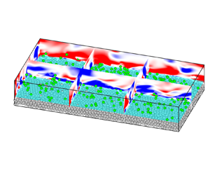
Figure 3 shows an instantaneous snapshot of two-phase flow after a statistically quasi-steady state is well established. The streamwise fluid velocity fluctuations  $u_f'=u_f-\langle u_f\rangle$ are illustrated in several $x\unicode{x2013}y$ and $z\unicode{x2013}y$ slices, depicting high- and low-speed streaks typically observed in wall turbulence. The entrained particles jump between quasi-streamwise vortices and instantaneously locate in either low- or high-speed streaks. However, on average, particles preferentially accumulate in the low-speed streaks (not shown here). The illustration on the right of figure 3 presents the wall-normal profile of the mean solid indicator fraction $\langle \varPhi \rangle$ defined by Kidanemariam et al. (Reference Kidanemariam, Chan-Braun, Doychev and Uhlmann2013), Kidanemariam & Uhlmann (Reference Kidanemariam and Uhlmann2014) and Kidanemariam & Uhlmann (Reference Kidanemariam and Uhlmann2017). Evidently, $\langle \varPhi \rangle$ is roughly divided into two parts along the height. In the lower part, the profile of $\langle \varPhi \rangle$ exhibits four bulges whose peak are $0.816$, $0.794$, $0.757$ and $0.533$, respectively. Note that the extreme value of the indicator fraction of densely packed particles on the stationary bed surface should be $0.816$ for hexagonal packing. In the upper part, however, a strong wall-normal particle concentration gradient forms due to the gravitational settling effect. The wall-normal location of the particle centres is overwhelming in the region of $y_p /H < 0.86$, where $y_p$ is the vertical height of the centre of the particle. The rolling and saltating of the particles generate an uneven bed surface, indicating a significant erosion phenomenon. The averaged fluid–bed interface location $H_b$ is extracted by means of a threshold value chosen as $\langle \varPhi (y_p)\rangle =0.1$ (Kidanemariam & Uhlmann Reference Kidanemariam and Uhlmann2014, Reference Kidanemariam and Uhlmann2017). In figure 3 the effective bed height of $H_b=0.34$ is clearly shown by a cyan transparent plane, on which a mean interface shear stress $\tau _b$ is defined by the sum of the viscous stress, Reynolds stress and drag feedback (Kidanemariam & Uhlmann Reference Kidanemariam and Uhlmann2017). Therefore, the friction Reynolds number $Re_\tau ^b=(H-H_b)u_{\tau }/\nu$ based on $H_f=H-H_b$ and the friction velocity $u_{\tau }$ defined as $=\sqrt {\tau _b/\rho _f}$ at $H_b$ is equal to $91$. Note that particles above and below the virtual interface are coloured green and grey, respectively.

Figure 3. Instantaneous snapshot of particle distribution. Several slices depict the streamwise fluid velocity fluctuation  $u_f'$. Particles above and below the mean interface height $H_b$ are labelled in green and grey, respectively. The inset on the right shows the average indicator fraction profile $\langle \varPhi \rangle$ of the solid particles. The top inset is the magnified view of the representative particle being tracked and its ambient flow at this moment.
At this moment, a representative ascending particle (the purple one) above  $H_b$ is selected for further Lagrangian tracing. The top inset of figure 3 is the magnified view of the representative particle being tracked and its ambient flow, in which the brown arrow marks out particle velocity. The smaller circles in the inset of figure 3 show the cross-section of surrounding particles on the $x\unicode{x2013}z$ plane through the centre of the tracked sphere. It can be seen that the tracked particle locates in the high-speed region of incoming flow at this moment. However, the fluid velocity behind the particle is very low due to the complicated wake and particle–particle interaction.
3.1. The drag force along saltating particle trajectory
We show the time series of the dynamic responses of the tracked particle during two successive saltation processes in figure 4. The abscissa  $t$ is non-dimensionalized by the inner scale of $\nu /u_\tau ^2$ and starts from the moment, $T_s$, that the particle is tracked and, therefore, $t^+=(T-T_s)u_\tau ^2/\nu$. The time interval for the data output is $\Delta t^+=0.146$.

Figure 4. Dynamic responses of a typical saltating particle within two successive trajectories. (a) The height of the particle centre  $y_p$, the local volume fraction around the tracked particle $\phi _p$ and the particle Reynolds number $Re_p$. (b) Time history of the streamwise component of the drag force. The solid black line is the PR-DNS results. The red, blue and green lines are the predicted results by models listed in table 1 respectively. (c,d) The same as (b), but for the wall-normal and spanwise components of the drag force.
Figure 4(a) depicts the vertical height (the red line) of the particle centre  $y_p$. It can be seen that the tracked particle reaches the vertexes of its parabolic-like trajectory at $t^+=32.26$ and $t^+=87.70$, and collides with other particles near the bed at $t^+=2.05$, $t^+=72.01$ and $t^+=114.10$. Note that the high and low trajectory vertexes are the direct results of different initial vertical take-off velocities for the two saltations. The local solid volume fraction $\phi _p$ (the blue line) and the particle Reynolds number $Re_p$ (the black line) are presented in the meanwhile. The same method as Link et al. (Reference Link, Cuypers, Deen and Kuipers2005) and Luo et al. (Reference Luo, Wang, Jin, Wang, Wang, Tan and Fan2021) is used to calculate $\phi_p$, that is $\phi _p=\sum _{\forall {j} \in {cell}}\alpha _{cell}^{j}V_{p,cell}^j/V_{cell}$, where $V_{p,cell}^j$ is the volume of a rectangular statistical cell around the particle, and $\alpha _{cell}^j$ is the ratio of the $j\mathrm {th}$ particle volume inside the statistical cell to the total particle volume. Here we use two different sizes of statistical cells to calculate $\phi _p$. The unit size of $4D_p\times 3D_p \times 3D_p$ is denoted as $\phi _p^{4\times 3 \times 3}$ and $5D_p\times 4D_p \times 4D_p$ is denoted as $\phi _p^{5\times 4 \times 4}$. For a finite-sized particle, the particle Reynolds number $Re_p$ cannot be defined unambiguously (Yu et al. Reference Yu, Lin, Shao and Wang2017) since there are different definitions of slip velocity $\boldsymbol {u}_{slip}=\boldsymbol {u}_f^*-\boldsymbol {u}_p$ between the individual particle and the ambient turbulent flow. When an individual particle is fixed ( $\boldsymbol {u}_p=0$) in an unbounded domain, $\boldsymbol {u}_{slip}$ can be simply taken to be the uniform inflow fluid velocity. In addition, the undisturbed flow velocity $\boldsymbol {u}_f^*$ in previous studies can also be the flow velocity at the particle centre, the flow velocity averaged over the particle surface based on the Faxén's theorem, the flow velocity at a particle size in front of the particle and the flow velocity averaged over a spherical shell centred at the particle location with radius of $R_s$ (Ganatos, Weinbaum & Pfeffer Reference Ganatos, Weinbaum and Pfeffer1980a; Ganatos, Pfeffer & Weinbaum Reference Ganatos, Pfeffer and Weinbaum1980b; Zeng et al. Reference Zeng, Balachandar, Fischer and Najjar2008; Cisse, Homann & Bec Reference Cisse, Homann and Bec2013; Akiki, Jackson & Balachandar Reference Akiki, Jackson and Balachandar2017a; Akiki, Moore & Balachandar Reference Akiki, Moore and Balachandar2017b; Li et al. Reference Li, Balachandar, Lee and Bai2019; Luo et al. Reference Luo, Wang, Tan and Fan2019, Reference Luo, Wang, Jin, Wang, Wang, Tan and Fan2021), and so on. Zeng et al. (Reference Zeng, Balachandar, Fischer and Najjar2008) argued that $\boldsymbol {u}_f^*$ at the particle centre is adequate for the small particle in predicting the instantaneous force but, for larger particles, a weighted volume average flow velocity over a small sphere centred around the particle location is better. Then Kidanemariam et al. (Reference Kidanemariam, Chan-Braun, Doychev and Uhlmann2013) first proposed a method based on an average of the fluid velocity over a trimmed spherical surface around a particle. Li et al. (Reference Li, Balachandar, Lee and Bai2019) also discussed the influence of different $\boldsymbol {u}_f^*$ definitions on the prediction of the force acting on a particle with different diameters and placed within different regions of wall turbulence. The performance of different definitions of $\boldsymbol {u}_f^*$ were revealed to be different. In the numerical simulation of a multiphase flow, it is especially difficult to determine the undisturbed fluid velocity seen by the particle since the flow has already been observably disturbed. We directly calculate $\boldsymbol {u}_f^*$ in this study according to Cisse et al. (Reference Cisse, Homann and Bec2013) and Luo et al. (Reference Luo, Wang, Tan and Fan2019, Reference Luo, Wang, Jin, Wang, Wang, Tan and Fan2021) based upon the mass flux entering a spherical shell. To be specific, a spherical shell with a radius of $R_s=3R_p$ is created by the Lagrangian grid generation scheme (Breugem Reference Breugem2012) and the fluid velocity can be easily interpolated to the Lagrangian grid by a trilinear interpolation method (Kidanemariam et al. Reference Kidanemariam, Chan-Braun, Doychev and Uhlmann2013; Chouippe & Uhlmann Reference Chouippe and Uhlmann2019). Then $\boldsymbol {u}_{slip}$ is calculated according to the averaging method proposed by Cisse et al. (Reference Cisse, Homann and Bec2013). The effects of $R_s$ will be discussed in § 5, as well as other typical $\boldsymbol {u}_f^*$ definitions.
It is seen from figure 4(a) that the local volume fraction around the particle  $\phi _p$ varies in the same way as $\langle \varPhi \rangle$ (above $H_b$) during its descending phase. Except for a visible plateau at approximately $8< t^+ < 15$ where another particle enters and stays in the statistical cell of $\phi _p$, there is no obvious qualitative difference between $\phi _p^{4\times 3 \times 3}$ and $\phi _p^{5\times 4 \times 4}$. Therefore, unless specifically stated in the following, the local volume fraction of particles $\phi _p$ is always represented by $\phi _p^{4\times 3 \times 3}$. On the contrary, the local volume fraction decreases rapidly during its ascending phase. One exception is the sudden weak bulge at approximately $t^+=50$, which should be attributed to the influence of bed particles since the tracked particle is now moving near the bed. The variation of the particle Reynolds number along its trajectory is a little bit complex however. Firstly, the smallest $Re_p$ can be observed near (but not exactly at) the vertexes of particle trajectories. This is to be expected since particles are much easier to be accelerated by the flow away from the bed, resulting in relatively small slip velocities. Secondly, $Re_p$ is very sensitive to the presence of the nearby particles. Taking the variation of $Re_p$ within $8< t^+< 15$ as an example, the particle Reynolds number continuously decreases through the fluid-mediated particle–particle interaction, but suddenly increases when the other particles move away. And finally, an abrupt change in $Re_p$ occurs before and after the collision, as shown during $t^+=0\sim 5$ and $t^+=50\sim 60$.
The solid black lines in figure 4(b–d) represent, respectively, the streamwise  $F_{D,x}$, wall-normal ( $F_{D,y}$) and spanwise ( $F_{D,z}$) components of the drag force acting on the tracked particle along its trajectory from PR-DNS, normalized by the submerged weight $G=(\rho _p-\rho _f))gV_p$. Note that the circles in these figures mark out the vertexes of the particle trajectory. We address here that the drag force $\boldsymbol {F}_D$ is the projection of the hydrodynamic force on the direction of slip velocity, namely, $\boldsymbol {F}_D=\boldsymbol {F}_h\cos \alpha _F$, where $\alpha _F$ is the angle between the hydrodynamic force $\boldsymbol {F}_h$ and slip velocity $\boldsymbol {u}_{slip}$. Several important features can be observed from the time history of the drag force. First, at each impact with the bed particles, the drag force peaks due to the collisions, which is consistent with that observed in Ji et al. (Reference Ji, Munjiza, Avital, Xu and Williams2014). Therefore, the maximum values of the $y$ coordinate are just $\pm 3$ in figure 4(b–d) to clearly show the drag force without collision. This sudden change is quickly damped by the hydrodynamic force. Second, there are sign changes of the drag force during both ascending and descending phases. However, the transition points of positive drag and negative drag force are not necessarily the same as the vertexes of the particle trajectory due to the complicated dynamics of turbulence–particle and particle–particle interactions. Third, the forces on the particle show substantial variations with time in addition to collision extremum during both ascending and descending phases; see, for example, $F_{D,z}$ during $21< t^+<45$ and $F_{D,y}$ during $40< t^+< 55$. In previous studies on individual fixed particles (Zeng et al. Reference Zeng, Balachandar, Fischer and Najjar2008; Homann et al. Reference Homann, Bec and Grauer2013; Li et al. Reference Li, Balachandar, Lee and Bai2019) these features cannot be observed at the same time.
In figure 4(b–d) we also show the drag forces predicted by several typical drag models based on the same  $\boldsymbol {u}_{slip}$ by DNS. The traditional drag models usually depend on $1\sim 3$ independent parameters to account for the different dynamics and parameter ranges. For the two-phase flow over the erodible bed concerned in this work, it is hard to distinguish the effects of the individual parameter. Since the mean/local shear, velocity fluctuation and the volume fraction all vary with wall-normal height in wall turbulence, we believe that the model that takes the particle-wall separation distance $L$ into account is a good choice, in addition to the models that involve $Re_p$ and $\phi _p$. The statistics indicate that the particle Reynolds number in the simulation falls in the range of $0< Re_p < 80$, and the solid volume fraction range is approximately $0< \phi _p < 0.25$ for saltating particles. Therefore, the standard drag model (Schiller & Nauman Reference Schiller and Nauman1935) of an isolated sphere that characterizes the Reynolds number dependence, the $\phi _p$-dependent model proposed by Tenneti et al. (Reference Tenneti, Garg and Subramaniam2011) and $L$-dependent model proposed by Zeng et al. (Reference Zeng, Najjar, Balachandar and Fischer2009) are employed for comparison. Throughout the paper, these three models are denoted as SN, TGS and Zeng model for short and the predicted drag forces are $\boldsymbol {F}_{D}^{SN}$, $\boldsymbol {F}_{D}^{TGS}$ and $\boldsymbol {F}_{D}^{Zeng}$. The drag coefficient $C_D$ of the three models are listed in table 1, according to which the drag force can be given as $\boldsymbol {F}_D=1/8{\rm \pi} \rho _f C_D D_p^2\lvert \boldsymbol {u}_{slip}\rvert \boldsymbol {u}_{slip}$. From figure 4 we can see that even though the models qualitatively capture the trend of PR-DNS results, the quantitative differences remain clear.
Table 1. Different drag force models. The predicted results from the SN, Zeng and TGS models, as shown in figure 4(b–d) and figure 8 as red, blue and green lines, respectively.

Before quantitatively evaluating the drag models, we collect and pretreat the PR-DNS data according to several subjective criteria. The bed particles are first excluded since we place emphasis on particles that characterize the two-phase flow over the erodible bed. Then, particles that meet  $H_{max,i}-H_{s,i}> 0.5D_p$ (Wiberg & Smith Reference Wiberg and Smith1985) and $y_p-D_p/2> H_b$ are identified as saltators, where $H_{max,i}$ and $H_{s,i}$ are the vertex of the $i\mathrm {th}$ saltating particle trajectory and particle initial take-off height, respectively. Note that the vertical position of the particle centre just finishes when the particle-bed collision is recorded as the initial take-off height of a saltating particle. From this moment (the initial take-off time, $t_{s,i}$) on, the $i\mathrm {th}$ particle moves in the fluid until falling back to the bed again at time $t_{e,i}$ due to gravity. All identified saltating trajectories are illustrated in figure 5(a) by their centre height, with regard to the inner-scale saltating time. Similar to Chouippe & Uhlmann (Reference Chouippe and Uhlmann2019), we define the saltating angle between the particle vertical velocity $u_{p,y}$ and the horizontal plane as $\beta =\mathrm {atan}(u_{p,y}/\sqrt {u_{p,x}^2+u_{p,z}^2})$, which can also be used to describe the particle saltation. Apparently, $\beta > 0$ indicates the ascending phase, $\beta < 0$ indicates the descending phase and the particle reaches the vertex of its trajectory when $\beta =0$. The probability density distribution of $\beta$ is plotted in figure 5(b). It can be seen that, for the saltation particle trajectory on the erodible bed surface in this study, $\beta$ is distributed between $-20^{\circ }$ and $40^{\circ }$.

Figure 5. (a) All identified saltating trajectories shown by the vertical height versus saltation time. (b) The probability density distribution of the saltating angle.
The model-predicted drag forces are then assessed using scatter plots and the correlation  $R^2$ values presented in figure 6, where $R^2$ is the statistical measure of how well the model prediction agrees with the actual PR-DNS data. By definition, a perfect model would have all the data points fall on the bisector, leading to $R^2=1$. With the decrease of $R^2$ to zero, the model predictions are completely irrelevant to PR-DNS results. For all frames, the abscissa and ordinate are for the PR-DNS and model-predicted results, respectively. Only streamwise and vertical components of the drag force are plotted in figure 6 since the spanwise component has similar comparison results as the streamwise component. In addition, the drag forces during descending and ascending phases are separately presented in consideration of the different dynamic responses shown in figure 4. Note that each point in the figure corresponds to the drag force on an individual particle at a given time, compared with the box-averaged pretreatment in several previous studies (Chen et al. Reference Chen, Song, Jiang, Ma and Zhou2020; Seyed-Ahmadi & Wachs Reference Seyed-Ahmadi and Wachs2020; Luo et al. Reference Luo, Wang, Jin, Wang, Wang, Tan and Fan2021).

Figure 6. Detail comparisons between model-predicted and PR-DNS drag force (non-dimensionalized by the submerged weight) in streamwise and vertical direction during descending  $u_{p,y}< 0$ and ascending $u_{p,y}> 0$ phases.
It can be seen from figure 6 that a number of scatters are in the second and fourth quadrants, which indicates that  $\alpha _F> 90^{\circ }$. In this case, the drag models cannot be improved by simple $C_D$ correction unless models are linearly superimposed with an additional contribution from the shear Reynolds number $Re_{\gamma }$ (Lee & Balachandar Reference Lee and Balachandar2010; Ekanayake et al. Reference Ekanayake, Berry, Stickland, Dunstan, Muir, Dower and Harvie2020, Reference Ekanayake, Berry and Harvie2021) and nearby particles (Akiki et al. Reference Akiki, Jackson and Balachandar2017a,Reference Akiki, Moore and Balachandarb), and so on. The correlation $R^2$ between the predictions and PR-DNS results vary from case to case. In general, $R^2$ during the ascending phase is higher than the descending phase, partly because the particles have a large initial kinetic energy after collision with bed particles, which makes them less susceptible to turbulence and the nearby particles. While during the settling stage, particles accelerated by gravity ( $F_{D,y}$ is applied almost in the opposite direction of motion) from zero $u_{p,y}$ are more prone to be influenced by neighbouring particles through the fluid-mediated interaction. The worst cases occur for $F_{D,y}$ during the descending phase, regardless of drag models. Here $R^2<0.2$ in $F_{D,y}$ frames indicates that PR-DNS results can hardly be predicted by the selected, typical drag models. We emphasize that the chaotic vortex shedding in the particle wake cannot be visibly observed at a relatively small particle Reynolds number (the maximum of $Re_p$ is smaller than $80$) in our simulation. In addition, it also shows that the volume fraction correction and particle-wall separation distance correction do improve the model predictions as compare to the classical SN model. Therefore, it is necessary to establish a new drag model appropriate for the two-phase flow based on the above comparisons.
3.2. A new drag model for saltating particle in two-phase flow
Unlike widely used drag models for a particle stationary or translating parallel to a wall developed in wall flow, it might be more appropriate to establish the drag model along its trajectory for a saltating particle. We assume that the local drag force for an isolated sphere can be well predicted by the  $C_D(Re_p)$ model, and the effect of other factors, the volume fraction, the particle-wall separation distance, turbulent velocity fluctuation and so on, are all integrated into a correction function $C_R$. Ideally, $C_R$ involves only dimensionless particle velocity, at least in addition to $Re_p$, and with a simple form for applications. It is not unreasonable since the particle-wall separation distance and the local volume fraction experienced by particles depend strongly on the velocity of the particle, as shown in figures 3 and 4. Consequently, the related turbulent structures (depending on whether the particle is embedded within the viscous sublayer, buffer region or the log layer) and the fluid-mediated particle–particle interaction are implicitly involved. Before fitting the $C_R \infty u_{p,y}$ relation, we try to give a brief discussion.
As described in Appendix A, we assume that the ratio of the work  $\int _{h_0}^{y_p}F_{h,y}{\cdot } \mathrm {d} y$ done by the hydrodynamic force component $F_{h,y}$ to the potential energy $(1-\rho _f/\rho _p)m_p(y_p-h_0)g$ is a constant according to the average energy and work plots (figure 12) and the initial position $h_0=0$, then we obtain the relationship for particle vertical velocity $u_{p,y}$ at height $y_p$, the initial vertical velocity $u_{p,0}$ and the vertex of a particle trajectory $h_s$ in dimensionless form as
 \begin{equation} y_p^+=h_s^+\left(1-u_{p,y}^2/u_{p,0}^2\right). \end{equation}
If the particle is placed in the viscous sublayer of wall turbulence, then  $y_p^+=u_f^+$, and the slip velocity is $\boldsymbol {u}_{slip}^+=\boldsymbol {u}_f^+-\boldsymbol {u}_{p}^+=[h_s^+(1-u_{p,y}^2/u_{p,0}^2)-u_{p,x}^+]\boldsymbol {e}_x-u_{p,y}^{+} \boldsymbol {e}_y$. If the particle is placed in the log layer of wall turbulence and the mean fluid velocity satisfies $u_f^+=({1}/{\kappa })\,\mathrm{ln}({y^+}/{y_0^+})$, where $\kappa$ and $y_0$ are the von Kármán constant and the bed roughness, respectively, then the saltating height can be expressed as $y_p^+=y_0^+( 1+\kappa u_f^+ +1/2\kappa ^2{u_f^+}^2+\cdots )$. As a result, the slip velocity can be expressed as $\boldsymbol {u}_{slip}^+=[{h_s^+}/{\kappa y_0^+}(1-u_{p,y}^2/u_{p,0}^2)-1/\kappa -u_{p,x}^+ ]\boldsymbol {e}_x-u_{p,y}^+\boldsymbol {e}_y$ by discarding higher-order terms. Nevertheless, such a rough discussion reveals that the slip velocity is approximately related to the $n$th power of the particle velocity. Let us assume that the relationship between $u_{slip}$ and $u_{p,y}$ can approximately be $u_{slip}=f(u_{p,y}^n)$, with $n$ ideally being approximately $2$. Putting the relation into the Stokes formula, we get the expression of drag force as
 \begin{equation} F_D=kf(u_{p,y}^n), \end{equation}
where  $k=3{\rm \pi} \rho _f D_p \nu$.
The standard drag curve of an isolated sphere characterizes  $Re_p$ dependence of the quasi-steady drag and is widely used as the benchmark mode for drag force corrections. We also use this scheme to develop the new drag force model. Figure 7(a) shows the ratio $\lvert \boldsymbol {F}_D \rvert / \lvert \boldsymbol {F}_D^{SN} \rvert$ of the PR-DNS drag forces to the drag forces predicted by the SN model as functions of $Re_p$ and $u_{p,y}/u_{p,0}$. Again, the points of $\lvert \boldsymbol {F}_D \rvert / \lvert \boldsymbol {F}_D^{SN} \rvert$ are very scattered when $Re_p$ or $u_{p,y}/u_{p,0}$ is fixed. It is hence unrealistic to directly pursue the instantaneous drag force in a real turbulence laden with saltating particles. We therefore divide the data into different $Re_p$ and $u_{p,y}/u_{p,0}$ bins. The widths of the bins are ${2.5}$ and ${0.25}$, respectively. Several typical $\lvert \boldsymbol {F}_D \rvert / \lvert \boldsymbol {F}_D^{SN} \rvert \infty {Re_p}$ and $\lvert \boldsymbol {F}_D \rvert / \lvert \boldsymbol {F}_D^{SN} \rvert \infty {u_{p,y}/u_{p,0}}$ curves are depicted in figure 7(b,c). It can be seen that $\lvert \boldsymbol {F}_D \rvert / \lvert \boldsymbol {F}_D^{SN} \rvert$ decreases with $Re_p$ monotonously but changes with $u_{p,y}/u_{p,0}$ quadratically. Then we use the least square method to fit the data and get the fitting formula of the drag coefficient as
 \begin{equation} \left. \begin{aligned} C_D^{Fit} & =C_D^{SN}C_R,\\ C_{R}\left(Re_p,\dfrac{u_{p,y}}{u_{p,0}}\right) & = \frac{40 {\left(\dfrac{u_{p,y}}{u_{p,0}}\right)} ^2 + 27 }{Re_p} . \end{aligned} \right\} \end{equation}
That is, the fitted drag coefficient is inversely proportional to  $Re_p$ and proportional to the particle speed squared. The fitted $C_R$ is shown in figure 7(a) as a transparent surface. Note that the applicability of (3.3) is limited. On the one hand, the ranges of the used parameter are $0< Re_p<80$ and $-2.0< u_{p,y}/u_{p,0}<2.0$. Making further simulations for different values of $D_p^+$ and particle-to-fluid density ratios will extend the parameter range of the model. However, it is challenging because the Shields number will change as well, resulting in varying erodibility of the bed. On the other hand, sediment in the bed-load layer is actually transported via several modes: rolling/sliding and saltating. Saltation is the most dominant for the formation of a two-phase flow in the current case. According to the above data pretreatment and fitting process, we stress again that the proposed model is only applicable to saltating particles that have a parabola-like trajectory as shown in figure 5(a). In an Euler–Lagrange simulation of a two-phase flow formed by saltating particles, if the bed is not resolved, a splashing function is usually employed to determine the bed particle's lift-off velocity and angle after a particle-bed collision (Zheng et al. Reference Zheng, Feng and Wang2021; Zhu et al. Reference Zhu, Hu, Lei, Shen and Zheng2022). Therefore, the initial vertical velocity $u_{p,0}$ can be easily obtained. Then, the new model can be adopted for the trajectory simulation.

Figure 7. A comparison between the drag force obtained by PR-DNS and SN model as a function of  $Re_p$ with ${u_{p,y}}/{u_{p,0}}$.
The mean drag forces  $\tilde {\boldsymbol {F}}_D$ along a particle trajectory predicted by the newly proposed model are plotted in figure 8, and compared against the PR-DNS results. Note that ‘along a particle trajectory’ here implies an average over the saltating angle $\beta$. The previous estimations that used particle-wall separation distance and volume fraction correction are also plotted in the same figure. The predictions from (3.3) agree well with the PR-DNS results, while the SN model underestimates the drag force on saltating particles the most even at the vertex of the trajectory where $L$- and $\phi _p$-dependence are relatively low. We attribute this underestimation towards the nonlinear force-velocity relation. The turbulent velocity fluctuation will increase the mean drag force predicted by the SN model according to the analysis of Zeng et al. (Reference Zeng, Balachandar, Fischer and Najjar2008). The TGS and Zeng models that involve, respectively, the correction of $\phi _p$ and $L$ both improve the predictions to a certain extent. When $\beta > 10^{\circ }$, the Zeng model performs better than the TGS model, which means that the effect of local solid volume fraction is less significant near the bed during the ascending phase. While for $\beta < -10^{\circ }$, the TGS model predictions are more consistent with DNS. Note that very close to the bed, (3.3) predictions still deviate from DNS. This may be attributed to the deviation of saltating particle trajectory from the smooth parabola near the bed due to the presence of rolling particles. Consequently, the relationship between $\boldsymbol {F}_D$ and $u_{p,y}$ for $\lvert u_{p,y}/u_{p,0}\rvert >1$ in figure 7(c) cannot be described by a quadratic function. This deviation can be eliminated to some degree by fitting the filtered data with $u_{p,y}/u_{\tau }$, see the orange dashed line, though the underlying physics is not as clear as $u_{p,y}/u_{p,0}$ when describing a particle trajectory.

Figure 8. The mean drag force along particle trajectories in a two-phase flow over an erodible bed.
4. Discussion
As discussed in § 3, there are different definitions of the undisturbed flow velocity  $\boldsymbol {u}_f^*$ in previous studies. We calculate $\boldsymbol {u}_{slip}$ according to Cisse et al. (Reference Cisse, Homann and Bec2013) with a radius of $R_s=3R_p$. However, the radius $R_s$ of the spherical shell may affect $\boldsymbol {u}_{slip}$. We perform an additional elaboration with $R_s=2R_p$ to evaluate the effects of $R_s$ on the drag force. Figure 9(a) shows the DNS drag force along the trajectories of the same particle as in figure 4 with different $R_s$. In addition, we also calculate the slip velocity based on the undisturbed flow velocity averaged over the $R_s=3R_p$ and $2R_p$ surface as Kidanemariam et al. (Reference Kidanemariam, Chan-Braun, Doychev and Uhlmann2013) and show the corresponding drag forces $\boldsymbol {F}_D^{Kid,3R_p}$ and $\boldsymbol {F}_D^{Kid,2R_p}$ in figure 9(a). Other methods for calculating the slip velocity, like the velocity at a point located one diameter in front of the particle and the undisturbed flow velocity at the particle centre from a companion DNS in the absence of particles, are either difficult to obtain or inappropriate. It is clear that the PR-DNS results are not very sensitive to $R_s$ for both methods, as shown in figure 9(b). In the process of saltation, the drag forces obtained by the two methods are similar in the general trend, but quantitative differences remain especially when the particles take off from the bed after the collision. Here $\boldsymbol {F}_D^{Kid,3R_p}$ and $\boldsymbol {F}_D^{Kid,2R_p}$ drop rapidly to near zero and then increase to the level of $\boldsymbol {F}_D$. Moreover, the fluctuation of drag force ${\sigma }_D^{Kid,3R_p}$ and ${\sigma }_D^{Kid,2R_p}$ seems to be smaller than ${\sigma }_D$ when $\beta >10^{\circ }$. Unfortunately, the underlying mechanics of the difference is not clear.

Figure 9. (a) Time histories of the drag force acting on the tracked particle in figure 4 based on different methods for calculating the slip velocity. (b) The fluctuating variances of the drag force along a particle trajectory.
Let us move to the underlying dynamics of the drag force. It is clear that the forces on the particle are caused by the complicated dynamics of turbulence–particle and particle–particle interactions. Figure 10 shows snapshots of the fluid velocity fluctuation and vorticity around the particle at  $t^+=44.00$, $t^+=46.93$ and $t^+=52.79$ to discern the influences. One can refer to figure 4 for the details along a particle trajectory. The brown, green and cyan arrows indicate the particle velocity, the slip velocity and hydrodynamic force, respectively. Within such a short time, the tracked particle is located in a somewhat high-speed streak, as shown in figure 10(a,c,e). Note that the low-speed wake behind the particle (the particle is large enough to create a wake behind it) interacts with turbulence, making it difficult to identify whether it is in a high-speed or low-speed streak. However, the streamwise component of the slip velocity is negative, indicating that the flow in front of the particle as it approaches the particle is high speed. At $t^+=44.00$, there is another nearby particle at the lower right of the tracked particle in figure 10(b). A positive local streamwise vorticity $\varOmega _x$ region between the two particles is visible. This region becomes intense and elongates as the other particle comes closer at $t^+=46.93$ in figure 10(d). While at $t^+=52.79$, $\varOmega _x$ shows an almost symmetrical, positive/negative vorticity region near the upstream face of the particle in figure 10(f) when the nearby particle moves away. We emphasize that the approaching particle leads to a dramatic change in both hydrodynamic force and $\alpha _F$ in figure 10(b,d,f).

Figure 10. Snapshots of the streamwise fluid velocity fluctuation  $u_f'$ in the $x- z$ plane at (a) $t^+=44.00$, (b) $t^+=46.93$, (c) $t^+=52.79$. The spanwise vorticity $\varOmega _x$ in the $z- y$ plane at the same time are presented in (b,d,f), respectively. The brown, green and cyan arrows indicate the particle velocity, the slip velocity and hydrodynamic force, respectively. The length of the arrows indicate the value of the variables.
Obviously, the inclusion of the local volume fraction in the drag model cannot effectively improve the prediction of the drag force since the force on the particle related to the local volume fraction will be estimated to be the same as long as  $\phi _p$ is the same within a given statistical box. This has already been confirmed by Akiki et al. (Reference Akiki, Jackson and Balachandar2017a) who further proposed a pairwise interaction extended point-particle model to account for the precise location of a few surrounding neighbours. The performance of this model was then validated by successfully simulating the sedimentation problems of $2$,
$2$,  $5$ and $80$ sediment spheres with the DEM method. A pairwise interaction assumed that each adjacent disturbance flow is independent, then the effects of all neighbours are linearly superposed to obtain the total perturbation based on the pre-stored single neighbour, $Re_p$-dependent perturbation libraries. However, in a two-phase turbulent flow over the erodible bed, the single neighbour perturbation libraries also depend on the position of all neighbours themselves.
Finally, we address here that the drag force is defined as the hydrodynamic force in the direction of the slip velocity following Luo et al. (Reference Luo, Wang, Jin, Wang, Wang, Tan and Fan2021), which indicates that the unsteady effects are implicitly involved (at least partially) in the modified drag force. Similar treatment was also done by Bombardelli, Picano & Brandt (Reference Bombardelli, Picano and Brandt2016) who considered the drag coefficient  $C_D$ as a function of the Reynolds number and Strouhal number (the unsteady effect). In the traditional view (Maxey & Riley Reference Maxey and Riley1983), the hydrodynamic forces on an individual point particle can be written as the sum of the quasi-steady (the drag force), stress-gradient, added-mass and viscous-unsteady forces (the Basset force), etc. It is natural to wonder if the inclusion of the unsteady forces can improve the prediction since there are rapid changes in the force that are due to the rapid changes in particle motion (Zeng et al. Reference Zeng, Balachandar, Fischer and Najjar2008; Li et al. Reference Li, Balachandar, Lee and Bai2019). To this end, we subtract the fluid acceleration force $\boldsymbol {F}_{FA}$, the added-mass force $\boldsymbol {F}_{AM}$ and the Basset history force $\boldsymbol {F}_{BA}$ from the total hydrodynamic force $\boldsymbol {F}_{h}$ to obtain the quasi-steady force $\boldsymbol {F}_{Steady}\ (=\boldsymbol {F}_{h}-\boldsymbol {F}_{FA}-\boldsymbol {F}_{AM}-\boldsymbol {F}_{BA})$. According to the Maxey–Riley equation (Maxey & Riley Reference Maxey and Riley1983), $\boldsymbol {F}_{FA}$, $\boldsymbol {F}_{AM}$ and $\boldsymbol {F}_{BA}$ on a solid particle can be expressed as
 \begin{equation} \left. \begin{aligned}
\boldsymbol{F}_{FA} & = \rho_f \frac{m_p}{\rho_p}
\frac{\mathrm{D}\boldsymbol{u}_f}{\mathrm{D}t}, \\ \boldsymbol{F}_{AM} &
= \frac{1}{2}\rho_f \frac{m_p}{\rho_p}
\left(\frac{\mathrm{D}\boldsymbol{u}_f}{\mathrm{D}t}-\frac{\mathrm{D}\boldsymbol{u}_p}{\mathrm{D}t} \right) ,\\ \boldsymbol{F}_{BA} & =
\frac{6{\rm \pi}\mu(D_p/2)^2}{\sqrt{{\rm \pi}\mu/\rho_f}} \left[
\int_{0}^t K(t-\tau) \left(
\frac{\mathrm{d}\boldsymbol{u}_f}{\mathrm{d}t}-\frac{\mathrm{d}\boldsymbol{u}_p}{\mathrm{d}t} \right) \,\mathrm{d}\tau\right], \end{aligned} \right\}
\end{equation}
\begin{equation} \left. \begin{aligned}
\boldsymbol{F}_{FA} & = \rho_f \frac{m_p}{\rho_p}
\frac{\mathrm{D}\boldsymbol{u}_f}{\mathrm{D}t}, \\ \boldsymbol{F}_{AM} &
= \frac{1}{2}\rho_f \frac{m_p}{\rho_p}
\left(\frac{\mathrm{D}\boldsymbol{u}_f}{\mathrm{D}t}-\frac{\mathrm{D}\boldsymbol{u}_p}{\mathrm{D}t} \right) ,\\ \boldsymbol{F}_{BA} & =
\frac{6{\rm \pi}\mu(D_p/2)^2}{\sqrt{{\rm \pi}\mu/\rho_f}} \left[
\int_{0}^t K(t-\tau) \left(
\frac{\mathrm{d}\boldsymbol{u}_f}{\mathrm{d}t}-\frac{\mathrm{d}\boldsymbol{u}_p}{\mathrm{d}t} \right) \,\mathrm{d}\tau\right], \end{aligned} \right\}
\end{equation}
The operator  $\mathrm {D}(.)/\mathrm {D}t$ indicates the material derivative, $K$ is the Basset kernel and $\tau$ is a dummy. Following Bombardelli, González & Niño (Reference Bombardelli, González and Niño2015), a memory time period concept is applied for the Basset kernel as
 \begin{equation} K(t-\tau) = \left\{ \begin{array}{@{}ll} \dfrac{1}{\sqrt{t-\tau}}, & t-t_{window}<\tau< t, \\ 0, & \tau< t-t_{window}.\\ \end{array} \right. \end{equation}
The projection of this quasi-steady hydrodynamic force component on the slip direction yields the quasi-steady drag force of  $\boldsymbol {F}_{D,Steady} = \boldsymbol {F}_{Steady}\cos {\alpha _F}$. The detail comparisons between SN-model-predicted drag force and $\boldsymbol {F}_{D,Steady}$ are presented in figure 11. Unfortunately, as compared with figure 6(a i–d i), $R^2$ is not fundamentally improved, which might be attributed to particle rotation taking place at anytime and anywhere along its trajectory.

Figure 11. The comparisons between the SN-model-predicted drag force and the quasi-steady drag force during the descending  $u_{p,y}<0$ and ascending $u_{p,y}>0$ phases.
5. Conclusions
In this study, particle saltation over the erodible bed in a turbulent open channel flow was numerically investigated using the DNS for turbulence flow, the fully resolved method and ACTM for particle dynamics and the IBM for the fluid–particle interaction. The drag force on saltating particles was presented along the particle trajectory. Typical drag models were employed to predict the drag force and compared against the PR-DNS results. According to the comparisons and the analysis on particle dynamics, a novel mean drag force model was proposed.
The particle volume fraction decreases rapidly along the height above the fluid–bed interface. Therefore, a saltating particle experiences a varying local volume fraction during its ascending and descending phases. Apart from inter-particle collision, the varying number of neighbouring particles, the turbulence structures around particles and the wake behind them make the drag force acting on particles in two-phase flow extremely complex. The typical SN model that characterizes the particle Reynolds number  $Re_p$ dependence, the TGS model that accounts for the joint influence of $Re_p$ and local volume fraction $\phi _p$, and the Zeng model that involves both $Re_p$ and the particle-wall separation distance $L$, are employed to examine if these models are still accurate enough to predict the drag force on a particle in a turbulent flow over the erodible bed. It is found that these classical models originally developed for a single particle cannot predict accurately the drag force acting on saltating particles, especially during their descending phase.
Through simple theoretical analysis of particle velocity and slip velocity along a particle trajectory, we proposed that the drag force should be a function of particle vertical velocity to the  $n$th power. Based on this consideration, we fitted the mean drag force along a particle trajectory, taking the SN model as the benchmark model. The trajectory was described by the angle $\beta$ between the particle vertical velocity and the horizontal plane. The corrected factor $C_R$ for the drag force is inversely proportional to $Re_p$ and proportional to the particle velocity (scaled by the initial take-off velocity $u_{p,0}$) squared. In addition, it is found that the performance of the new drag model can be further improved if the particle vertical velocity $u_{p,y}$ in the corrected factor is scaled by the friction velocity $u_{\tau }$ of the two-phase flow.
Due to the complicated combined influence of turbulence–particle and particle–particle interactions on particle dynamics, it is not possible so far to study the fluctuation of the drag force just based on  $u_{p,y}$ and $Re_p$. Furthermore, the particle-to-fluid density ratio, the particle-to-fluid scale ratio, the Shield number and the turbulence Reynolds number will all play pivotal roles in the prediction of the drag force.
Acknowledgements
We thank the three anonymous referees for their useful comments.
Funding
X.J.Z. and Z.P.Z. are supported by the National Natural Science Foundation of China (grant number 92052202). P.W. and Y.H.N.L. are supported by the National Natural Science Foundation of China (grant number 12072138) and National Numerical Windtunnel project.
Declaration of interests
The authors report no conflict of interest.
Appendix A
The motion equation of particles (without collision force) in the vertical direction is
 \begin{equation} m_p \frac{\mathrm{d}u_{p,y}}{\mathrm{d}t}=V_p(\rho_p-\rho_f)g+F_{h,y}, \end{equation}
where  $V_p$ and $F_{h,y}$ are the volume of the spheroidal particle and the vertical component of the hydrodynamic force. The works done by each term after distance $\mathrm {d} y=u_{p,y}\,\mathrm {d}t$ are
 \begin{equation} m_p \frac{\mathrm{d}u_{p,y}}{\mathrm{d}t} \cdot u_{p,y}\,\mathrm{d} t = V_p(\rho_p-\rho_f)g \cdot \,\mathrm{d} y + F_{h,y} \cdot \mathrm{d} y. \end{equation}
By integrating the above equation from 0 to  $t$ (from $h_0$ to $y_p$),
 \begin{equation} \int_0^{t} m_p \frac{\mathrm{d}u_{p,y}}{\mathrm{d}t} \cdot u_{p,y}\,\mathrm{d} t = \int_{h_0}^{y_p} V_p(\rho_p-\rho_f)g \cdot \mathrm{d} y + \int_{h_0}^{y_p} F_{h,y} \cdot \mathrm{d} y, \end{equation}
we can get
 \begin{equation} m_p \left(\frac{u_{p,y}^2}{2} - \frac{u_{p,0}^2}{2}\right) = V_p(\rho_p-\rho_f)g \cdot (y_p-h_0) + \int_{h_0}^{y_p}F_{h,y} \cdot \mathrm{d} y \end{equation}
or
 \begin{equation} m_p \left(\frac{u_{p,y}^2}{2} - \frac{u_{p,0}^2}{2}\right) = (1-\rho_f/\rho_p)m_p(y_p-h_0)g + \int_{h_0}^{y_p}F_{h,y} \cdot \mathrm{d} y. \end{equation}
At the vertex  $h_s$ of a particle trajectory, we have
 \begin{equation} - \frac{1}{2}m_p u_{p,0}^2 = (1-\rho_f/\rho_p)m_p(h_s-h_0)g + \int_{h_0}^{h_s}F_{h,y} \cdot \mathrm{d} y. \end{equation}
 \begin{equation} 1 - \frac{u_{p,y}^2}{u_{p,0}^2} = \frac{(1-\rho_f/\rho_p)m_p(y_p-h_0)g + \int_{h_0}^{y_p}F_{h,y} \cdot \mathrm{d} y} {(1-\rho_f/\rho_p)m_p(h_s-h_0)g + \int_{h_0}^{h_s}F_{h,y} \cdot \mathrm{d} y}. \end{equation}
The kinetic energy, potential energy and the work done by the hydrodynamic force component  $F_{h,y}$ along a particle trajectory are plotted in figure 12. It is found that the ratio $E_{ratio}$ of $\int _{h_0}^{y_p}F_{h,y} {\cdot } \mathrm {d} y$ to $(1-\rho _f/\rho _p)m_p(y_p-h_0)g$ is approximately 0.0–0.5 except for $\beta <-12^{\circ }$ (particles settle near the bed surface) and $\beta >25^{\circ }$ (where the probability density distribution of $\beta$ is low). Although the ratio varies with $\beta$, let us assume that the ratio $E_{ratio}$ is equal to a constant value $B$ and the right-hand side of (A7) becomes
 \begin{equation} \frac{(1-\rho_f/\rho_p)m_p(y_p-h_0)g +B (y_p-h_0)} {(1-\rho_f/\rho_p)m_p(h_s-h_0)g + B(h_s-h_0)}. \end{equation}
Then, the simple theoretical analysis and assumption yield
 \begin{equation} \frac{u_{p,y}^2}{u_{p,0}^2} \approx \frac{h_s-y_p} {h_s-h_0} . \end{equation}
Figure 12. (a) The kinetic energy, potential energy and work done by the vertical component of the hydrodynamic force along a particle trajectory, averaged over  $\beta$. (b) Ratio of the work done by the vertical component of the hydrodynamic force to potential energy.


