


1. Introduction
As discussed in detail in many books (Williams Reference Williams1985; Chomiak Reference Chomiak1990; Kuznetsov & Sabelnikov Reference Kuznetsov and Sabelnikov1990; Peters Reference Peters2000; Poinsot & Veynante Reference Poinsot and Veynante2005; Echekki & Mastorakos Reference Echekki and Mastorakos2011; Swaminathan & Bray Reference Swaminathan and Bray2011; Lipatnikov Reference Lipatnikov2012) and review articles (Borghi Reference Borghi1988; Bray Reference Bray1995, Reference Bray1996; Lipatnikov & Chomiak Reference Lipatnikov and Chomiak2002; Veynante & Vervisch Reference Veynante and Vervisch2002; Bilger et al. Reference Bilger, Pope, Bray and Driscoll2005; Lipatnikov & Chomiak Reference Lipatnikov and Chomiak2005; Driscoll Reference Driscoll2008; Lipatnikov & Chomiak Reference Lipatnikov and Chomiak2010; Sabelnikov & Lipatnikov Reference Sabelnikov and Lipatnikov2017; Driscoll et al. Reference Driscoll, Chen, Skiba, Carter, Hawkes and Wang2020; Klimenko Reference Klimenko2021; Steinberg, Hamlington & Zhao Reference Steinberg, Hamlington and Zhao2021), premixed turbulent combustion is a highly nonlinear and multiscale phenomenon, which involves (i) thousands of chemical reactions between hundreds of species, (ii) interactions between these reactions, heat release, molecular transport of the species and heat, and turbulent eddies of various scales as well as (iii) strongly localized density variations, which significantly affect the flow. Accordingly, a number of local phenomena stem from flame–turbulence interactions. Such effects are often explored by investigating local characteristics of reaction zones, sampled from direct numerical simulation (DNS) data obtained from various premixed turbulent flames. A list of such characteristics involves, but is not limited to, flame curvature, strain and stretch rates, displacement speed  $S_d$ and flame surface density $\varSigma$ (mathematical definitions and references are provided in § 2).
While a large amount of statistical information on the behaviour of these quantities in premixed turbulent flames has already been sampled from many DNS databases, such results are mainly limited either to single-step combustion chemistry or to mixtures characterized by approximately equal molecular diffusivities of fuel, oxygen and heat and, consequently, associated with weakly pronounced differential diffusion effects. However, currently, these effects draw lot of attention due to rapidly growing interest in utilizing chemical energy bound in renewable carbon-free fuels such as hydrogen. As the molecular diffusivity of H $_2$ is large, lean hydrogen–air flames are characterized by a low Lewis number $Le=a/D$, i.e. a ratio of the molecular heat diffusivity $a$ of a mixture to the molecular diffusivity $D$ of a deficient reactant in this mixture, with significant influence of $Le$ on turbulent burning rate being documented in experiments by Wohl & Shore (Reference Wohl and Shore1955), Karpov & Sokolik (Reference Karpov and Sokolik1961), Karpov & Severin (Reference Karpov and Severin1980), Abdel-Gayed et al. (Reference Abdel-Gayed, Bradley, Hamid and Lawes1984), Kido et al. (Reference Kido, Kitagawa, Nakashima and Kato1989) and Wu et al. (Reference Wu, Kwon, Driscoll and Faeth1990), and in many other measurements reviewed elsewhere (Kuznetsov & Sabelnikov Reference Kuznetsov and Sabelnikov1990; Lipatnikov & Chomiak Reference Lipatnikov and Chomiak2005; Lipatnikov Reference Lipatnikov2012). Recently, an extremely high magnitude of such differential diffusion effects was reported by Yang et al. (Reference Yang, Saha, Liang, Wu and Law2018).
From the qualitative perspective, the highlighted sensitivity of turbulent burning rate to differences in molecular transport coefficients is known to stem from variations in the local temperature and mixture composition due to imbalance of reactant and heat fluxes to/from thin reaction zones strained and curved by turbulent eddies (Kuznetsov & Sabelnikov Reference Kuznetsov and Sabelnikov1990; Bradley, Lau & Lawes Reference Bradley, Lau and Lawes1992; Lipatnikov & Chomiak Reference Lipatnikov and Chomiak2005; Lipatnikov Reference Lipatnikov2012). Such variations are expected to significantly affect not only burning rate, but also other local flame characteristics such as  $S_d$ and $\varSigma$. However, behaviour of displacement speed or flame surface density has not yet been thoroughly investigated in highly turbulent lean hydrogen–air mixtures characterized by a low Lewis number and the present work aims at bridging this knowledge gap by analysing recent DNS data.
In § 2, required mathematical background is summarized and specific research goals are stated. An overview of the DNS attributes is presented in § 3. Numerical results are reported and discussed in § 4, followed by concluding remarks.
2. Background and research goals
Premixed turbulent combustion is commonly modelled (Bray Reference Bray1995, Reference Bray1996; Peters Reference Peters2000; Bilger et al. Reference Bilger, Pope, Bray and Driscoll2005; Poinsot & Veynante Reference Poinsot and Veynante2005; Lipatnikov Reference Lipatnikov2012) invoking the following transport equations:
 \begin{equation} \rho \frac{\partial \psi_k}{\partial t} + \rho \boldsymbol{u}\boldsymbol {\cdot }\boldsymbol{\nabla} \psi_k + \boldsymbol{\nabla}\boldsymbol{\cdot} \boldsymbol{J}_{\psi,k} = \dot{\omega}_{\psi,k} \end{equation}
for a set  $\boldsymbol {\psi }=\{\psi _1, \ldots, \psi _N \}$ of scalar characteristics of mixture state in a premixed flame, e.g. mass fractions $Y_l$ of various species, temperature $T$, etc. Here, $t$ designates time; $\rho$ is the density; $\boldsymbol {u}$ is the flow velocity vector; and $\boldsymbol {J}_{\psi,k}$ and $\dot {\omega }_{\psi,k}$ designate the molecular flux of the scalar $\psi _k$ and the rate of its creation, respectively. When developing models of the influence of turbulence on premixed burning, the set $\boldsymbol {\psi }$ is often reduced to a single combustion progress variable $c$, which is equal to zero and unity in unburned reactants and burned products, respectively, and can be defined by properly normalizing temperature or concentration of a major reactant or product (Bray Reference Bray1995, Reference Bray1996; Peters Reference Peters2000; Bilger et al. Reference Bilger, Pope, Bray and Driscoll2005; Poinsot & Veynante Reference Poinsot and Veynante2005; Lipatnikov Reference Lipatnikov2012). For brevity, equations summarized in the present section address this simplest case, but the equations can easily be extended to a more general case, e.g. if the set $\boldsymbol {\psi }$ involves normalized concentrations of fuel and oxidant, as well as normalized temperature.
In the chosen simplest case, a local displacement speed  $S_d$ is defined as follows (Gibson Reference Gibson1968; Pope Reference Pope1988; Gran, Echekki & Chen Reference Gran, Echekki and Chen1996):
 \begin{equation} S_d \equiv \frac{- \boldsymbol{\nabla}\boldsymbol{\cdot} \boldsymbol{J}_c + \dot{\omega}_c}{\rho |\boldsymbol{\nabla} c|} \end{equation}
or
 \begin{equation} S_d = \underbrace{\frac{\dot{\omega}_c}{\rho |\boldsymbol{\nabla} c|}}_{T_1} + \underbrace{\frac{\boldsymbol{n} \boldsymbol{\cdot}\boldsymbol{\nabla} (\rho D_c \boldsymbol{n} \boldsymbol{\cdot} \boldsymbol{\nabla} c)}{\rho |\boldsymbol{\nabla} c|}}_{T_2} \underbrace{- D_c \boldsymbol{\nabla}\boldsymbol{\cdot}\boldsymbol{n}}_{T_3} \end{equation}
if Fickian law is adopted to model the flux  $\boldsymbol {J}_c = - \rho D_c \boldsymbol {\nabla } c$. Here, $\boldsymbol {n} = - \boldsymbol {\nabla } c/|\boldsymbol {\nabla } c|$ is the unit vector normal to the iso-surface $c(\boldsymbol {x},t)={\rm const.}$ and pointing to fresh mixture; $D_c$ is molecular diffusivity of $c$; and terms $T_1$, $T_2$ and $T_3$ are associated with reaction, normal diffusion and tangential diffusion, respectively.
The displacement speed is widely used in the premixed turbulent combustion literature for a number of reasons. First,  $S_d$ can easily be sampled from DNS data using either (2.2) or
 \begin{equation} S_d = \frac{1}{|\boldsymbol{\nabla} c|} \left( \frac{\partial c}{\partial t} + \boldsymbol{u} \boldsymbol{\cdot}\boldsymbol{\nabla} c \right). \end{equation}
 Second, in an unperturbed (stationary, planar and one-dimensional) laminar premixed flame, the continuity equation, (2.1) with  $\psi =c$ and (2.3) directly yield
 \begin{equation} \rho_u S_L = \rho u = \rho S_d = \rho_u S_d^* = \int_{-\infty}^{\infty} \dot{\omega}_c \,\mathrm{d}\kern0.06em x , \end{equation}
i.e. the density-weighted value
 \begin{equation} S_d^* \equiv \frac{\rho S_d}{\rho_u} \end{equation}
of displacement speed is equal to the unperturbed laminar flame speed  $S_L$ and to burning (or consumption) velocity $\int _{-\infty }^{\infty } \dot {\omega }_c\, \mathrm {d}\kern 0.06em x/\rho _u$ everywhere within such a flame. Here, subscript ‘ $u$’ refers to unburned reactants.
Third, substitution of (2.2) into (2.1) results in the following kinematic equation:
 \begin{equation} \frac{\partial c}{\partial t} + \left( \boldsymbol{u} + S_d \boldsymbol{n} \right) \boldsymbol{\cdot} \boldsymbol{\nabla} c = 0. \end{equation}
Therefore, displacement speed of the iso-scalar surface  $c(\boldsymbol {x},t)=\xi$ is equal to the speed of this surface with respect to the local flow. Accordingly, difference in $S_L$ and $S_d^*$ conveys information on the influence of turbulence on the local flame speed.
Fourth, multiplication of (2.2) with  $\rho |\boldsymbol {\nabla } c|$ and spatial integration of the obtained equation yield
 \begin{equation} \int\!\!\int\!\!\int\,\rho S_d |\boldsymbol{\nabla} c| \,\mathrm{d} \boldsymbol{x} =- \int\!\!\int\!\!\int\,\boldsymbol{\nabla}\boldsymbol{\cdot} \boldsymbol{J}_c \,\mathrm{d}\boldsymbol{x} + \int\!\!\int\!\!\int\,\dot{\omega}_c \,\mathrm{d}\boldsymbol{x} \end{equation}
or
 \begin{equation} \int\!\!\int\!\!\int\,\rho S_d |\boldsymbol{\nabla} c| \,\mathrm{d}\boldsymbol{x} = \int\!\!\int\!\!\int\,\dot{\omega}_c \,\mathrm{d}\boldsymbol{x} \end{equation}
if molecular fluxes through opposite boundaries of the considered spatial domain are equal to one another, as occurs in a typical DNS study. Thus, there is a direct link between displacement speed and bulk burning rate  $\int \!\!\int \!\!\int \,\dot {\omega }_c \,\mathrm {d}\boldsymbol {x}$. Furthermore, in the simplest case of a statistically planar and one-dimensional flame normal to the $x$ axis, which is considered in the rest of the present paper unless otherwise stated, (2.9) reads
 \begin{equation} \int_{-\infty}^{\infty} \overline{\rho S_d |\boldsymbol{\nabla} c|} \,\mathrm{d}\kern0.06em x = \int_{-\infty}^{\infty} \overline{\dot{\omega}_c} \,\mathrm{d}\kern0.06em x \equiv \rho_u U_T, \end{equation}
where an overline designates a transverse average. Thus, the integrated product  $\overline {\rho S_d |\boldsymbol {\nabla } c|}$ directly characterizes turbulent burning velocity $U_T$, similarly to the integrated mean rate $\overline {\dot {\omega }_c}$.
Fifth, by introducing a flame-conditioned displacement speed
 \begin{equation} \langle \rho S_d \rangle_f \equiv \frac{\overline{\rho S_d |\boldsymbol{\nabla} c|}}{\overline{|\boldsymbol{\nabla} c|}}, \end{equation}
(2.10) can be rewritten as follows:
 \begin{equation} \int_{-\infty}^{\infty} \langle \rho S_d \rangle_f \overline{|\boldsymbol{\nabla} c|} \,\mathrm{d}\kern0.06em x = \rho_u \int_{-\infty}^{\infty} \langle S_d^* \rangle_f \overline{|\boldsymbol{\nabla} c|} \,\mathrm{d}\kern0.06em x = \rho_u U_T, \end{equation}
thus further emphasizing the link between turbulent burning velocity and displacement speed.
In the simplest case of  $\langle S_d^* \rangle _f=S_L$, i.e. if a local flame in a turbulent flow retains the structure of the unperturbed laminar flame or, in other words, the influence of turbulence on the local flame structure is negligible, (2.12) reads
 \begin{equation} U_T = S_L \int_{-\infty}^{\infty} \overline{|\boldsymbol{\nabla} c|} \,\mathrm{d}\kern0.06em x \equiv S_L A_{\sigma}. \end{equation}
The integral  $A_{\sigma }$ is associated with a relative increase $A_f$ in a turbulent flame surface area when compared with a planar laminar flame, because the quantity $\overline {|\boldsymbol {\nabla } c|}$ in this integral is known as the generalized flame surface density. Indeed, integrating the mean value $\overline {\varSigma _{\xi }}$ of flame surface density $\varSigma _{\xi } \equiv \delta (c-\xi ) |\boldsymbol {\nabla } c|$ (Pope Reference Pope1988) over $\xi$, one can arrive at (Vervisch et al. Reference Vervisch, Bidaux, Bray and Kollmann1995; Veynante & Vervisch Reference Veynante and Vervisch2002)
 \begin{equation} \int_0^1 \overline{\varSigma_{\xi}} \,\mathrm{d} \xi = \int_0^1 \overline{\delta(c-\xi) |\boldsymbol{\nabla} c|} \,\mathrm{d} \xi = \int_0^1 \langle |\boldsymbol{\nabla} c| | c=\xi \rangle P(\xi) \,\mathrm{d} \xi = \overline{|\boldsymbol{\nabla} c|}. \end{equation}
Here,  $\delta (c-\xi )$ is the Dirac delta function. Accordingly, the integral $A_{\sigma }$ on the right-hand side of (2.13) characterizes an increase in a generalized flame surface area and the influence of turbulence on a premixed flame is solely reduced to an increase in this area, in line with the first Damköhler hypothesis (Damköhler Reference Damköhler1940).
If the influence of turbulence on the local burning rate and flame structure is substantial so that  $\langle S_d^* \rangle _f \ne S_L$, (2.12) can be rewritten as follows:
 \begin{equation} U_T = S_L G_0 \int_{-\infty}^{\infty} \overline{|\boldsymbol{\nabla} c|} \,\mathrm{d}\kern0.06em x = S_L G_0 A_{\sigma}, \end{equation}
where
 \begin{equation} G_0 \equiv \frac{ \displaystyle\int\nolimits_{-\infty}^{\infty} \langle S_d^* \rangle_f \overline{|\boldsymbol{\nabla} c|} \,\mathrm{d}\kern0.06em x}{S_L \displaystyle\int\nolimits_{-\infty}^{\infty} \overline{|\boldsymbol{\nabla} c|} \,\mathrm{d}\kern0.06em x} \end{equation}
is a bulk stretch factor.
Sixth, displacement speed is often used not only to explore turbulent burning velocity  $U_T$ adopting (2.15) and (2.16), but also to respond to the major challenge of premixed turbulent combustion (Bray Reference Bray1996), i.e. to arrive at a closure relation for the mean rate $\overline {\dot {\omega }_c}$ of product creation. While (2.2) reads
 \begin{equation} \overline{\dot{\omega}_c} = \rho_u \overline{S_d^* |\boldsymbol{\nabla} c|} + \boldsymbol{\nabla} \boldsymbol{\cdot} \overline{\boldsymbol{J}_c} = \rho_u \langle S_d^* \rangle_f \overline{|\boldsymbol{\nabla} c|} + \boldsymbol{\nabla}\boldsymbol{\cdot}\overline{\boldsymbol{J}_c}, \end{equation}
the following approximate closure relation:
 \begin{equation} \overline{\dot{\omega}_c} = \rho_u \overline{u_c} \overline{\varSigma_{\xi}} = \rho_u S_L I_0 \overline{\varSigma_{\xi}} \end{equation}
is widely accepted in the premixed turbulent combustion literature (Bray Reference Bray1990, Reference Bray1996; Peters Reference Peters2000; Veynante & Vervisch Reference Veynante and Vervisch2002; Bilger et al. Reference Bilger, Pope, Bray and Driscoll2005; Poinsot & Veynante Reference Poinsot and Veynante2005; Lipatnikov Reference Lipatnikov2012). Here, a stretch factor  $I_0$ is introduced (Cant & Bray Reference Cant and Bray1988; Bray Reference Bray1990; Bray & Cant Reference Bray and Cant1991) to characterize a ratio of the mean local consumption velocity $\overline {u_c}$ to the laminar flame speed $S_L$ and the local consumption velocity $u_c$ (Bray Reference Bray1995, Reference Bray1996; Peters Reference Peters2000; Veynante & Vervisch Reference Veynante and Vervisch2002; Bilger et al. Reference Bilger, Pope, Bray and Driscoll2005; Poinsot & Veynante Reference Poinsot and Veynante2005; Lipatnikov Reference Lipatnikov2012) is a rate of product creation per unit flame surface area, divided by $\rho _u$, or the rate $\dot {\omega }_c/\rho _u$ integrated along the local normal to an infinitesimal flame element in the vicinity of it. This closure relation is based on the first Damköhler hypothesis and reduces the influence of turbulence on a premixed flame to (i) an increase in the flame surface area, characterized locally with $\overline {\varSigma _{\xi }}$, and (ii) a change in the local flame structure, characterized with the stretch factor $I_0$. Therefore, (2.18), in fact, extends the first Damköhler hypothesis by substituting $S_L$ with $\overline {u_c} = S_L I_0$. To adopt such an approach in applied simulations, a model of $I_0$ is required and research into displacement speed aims often at addressing this task by assuming that $S_L I_0$ may be substituted with an appropriately averaged $S_d^*$ in (2.18).
Thus, for the above reasons, statistical behaviour of  $S_d$ has been the focus of a number of DNS studies of premixed turbulent combustion. Some of them addressed correlations between $S_d$ or $S_d^*$ and (i) the local strain rate (Chakraborty & Cant Reference Chakraborty and Cant2004; Hawkes & Chen Reference Hawkes and Chen2006; Kim & Pitsch Reference Kim and Pitsch2007; Chaudhuri Reference Chaudhuri2015; Cecere et al. Reference Cecere, Giacomazzi, Arcidiacono and Picchia2016), (ii) the local flame curvature (Echekki & Chen Reference Echekki and Chen1996; Chakraborty & Cant Reference Chakraborty and Cant2004; Sankaran et al. Reference Sankaran, Hawkes, Yoo and Chen2015; Wang, Hawkes & Chen Reference Wang, Hawkes and Chen2017a; Wang et al. Reference Wang, Hawkes, Chen, Zhou, Li and Aldén2017b; Luca et al. Reference Luca, Attili, Schiavo, Creta and Bisetti2019), (iii) alignment characteristics of scalar gradient with principal strain rates (Chakraborty & Swaminathan Reference Chakraborty and Swaminathan2007) or (iv) flame-surface topology (Dopazo, Martín & Hierro Reference Dopazo, Martín and Hierro2007; Cifuentes et al. Reference Cifuentes, Dopazo, Martin, Domingo and Vervisch2014). In other DNS studies, probability density function of $S_d^*$ was investigated (Chakraborty, Klein & Cant Reference Chakraborty, Klein and Cant2007; Nivarti & Cant Reference Nivarti and Cant2017; Song et al. Reference Song, Hernández Pérez, Tingas and Im2021), behaviour of displacement speed conditioned to the local flame curvature was explored (Dave & Chaudhuri Reference Dave and Chaudhuri2020), various terms in an evolution equation for a bulk displacement speed were analysed (Yu et al. Reference Yu, Nilsson, Fureby and Lipatnikov2021), etc. Often, the far-reaching goal of such studies consists of arriving at simple model equations for evaluation of a mean value of $S_d^*$, which could substitute $\overline {u_c}$ in (2.18). Accordingly, the problem of predicting turbulent burning rate is split into two separate tasks: (i) modelling an increase in flame surface area and (ii) modelling the influence of turbulence on local flame speed. Equations sought to solve the latter problem are typically based on the theory of weakly perturbed laminar flames (Matalon & Matkowsky Reference Matalon and Matkowsky1982; Pelcé & Clavin Reference Pelcé and Clavin1982; Class, Matkowsky & Klimenko Reference Class, Matkowsky and Klimenko2003; Kelley, Bechtold & Law Reference Kelley, Bechtold and Law2012), with substantial progress in this research direction being recently made by Dave & Chaudhuri (Reference Dave and Chaudhuri2020).
However, it is worth remembering that the local values of  $S_d(\boldsymbol {x},t)$ can be widely scattered and irrelevant to the local burning rate. For instance, in the case of inert turbulent mixing, $S_d$ evaluated using (2.2) does not vanish, whereas $\dot {\omega }_c(\boldsymbol {x},t) \equiv 0$. On the contrary, on the surface of a stationary flame ball (Zel'dovich et al. Reference Zel'dovich, Barenblatt, Librovich and Makhviladze1985), $S_d$ vanishes in spite of a high rate $\dot {\omega }_c$. Furthermore, $S_d$ can be even negative, as predicted by Klimov (Reference Klimov1963) and documented by Gran et al. (Reference Gran, Echekki and Chen1996) and in a number of subsequent DNS studies (Chakraborty et al. Reference Chakraborty, Klein and Cant2007; Nivarti & Cant Reference Nivarti and Cant2017; Luca et al. Reference Luca, Attili, Schiavo, Creta and Bisetti2019; Yu & Lipatnikov Reference Yu and Lipatnikov2019; Song et al. Reference Song, Hernández Pérez, Tingas and Im2021; Berger, Attili & Pitsch Reference Berger, Attili and Pitsch2022). In addition, $S_d$ can tend to infinity in the vicinity of so-called ‘zero gradient points’ (Gibson Reference Gibson1968), e.g. somewhere in preheat zones of two colliding laminar flames. In such a case, large local values of $S_d$ do not indicate high local burning rates $\dot {\omega }_c$. In a general case, a local displacement speed does not characterize the local burning rate $\dot {\omega }_c$, because $S_d$ may be controlled by molecular mixing; see terms $T_2$ and $T_3$ in (2.3).
These fundamental issues are often circumvented by assuming that the local effects emphasized above are suppressed after averaging. Such an assumption appears to be sufficiently plausible if local variations in  $S_d^*$ and $u_c$ within reaction zones strained and wrinkled by turbulent eddies are weakly pronounced, e.g. see recent DNS studies by Dave & Chaudhuri (Reference Dave and Chaudhuri2020) or Song et al. (Reference Song, Hernández Pérez, Tingas and Im2021). However, such local variations can be significant if the Lewis number is low. In the latter case, local mixture composition, temperature and, hence, burning rate within reaction zones are significantly affected by the local imbalance of molecular flux of chemical energy to the zones and molecular heat flux from the zones. As reviewed elsewhere (Kuznetsov & Sabelnikov Reference Kuznetsov and Sabelnikov1990; Lipatnikov & Chomiak Reference Lipatnikov and Chomiak2005; Lipatnikov Reference Lipatnikov2012), such differential diffusion effects manifest themselves, e.g. in a large increase in turbulent burning velocity in very lean hydrogen–air mixtures characterized by a low Lewis number. Accordingly, there is a need for exploring behaviour of displacement speed in premixed turbulent flames characterized by a low $Le$ and the present work aims at bridging this knowledge gap.
In this regard, it is worth noting that mean values of displacement speed or flame surface density can be evaluated adopting different methods even in the simplest case of a statistically stationary, one-dimensional and planar mean flame brush addressed here. In particular, if conventionally (time and/or transverse) averaged  $\overline {|\boldsymbol {\nabla } c|}$ is considered to measure flame surface density, two different mean values of $S_d^*$, i.e. $\overline {S_d^*}$ or $\langle S_d^* \rangle _f$, can be obtained either by taking the same conventional average or applying (2.11), respectively. For instance, conventionally averaged displacement speed $S_d^*$ was used by Chakraborty & Cant (Reference Chakraborty and Cant2005b), Dave & Chaudhuri (Reference Dave and Chaudhuri2020) and Lu & Yang (Reference Lu and Yang2020), the flame-conditioned $\langle S_d^* \rangle _f$ was adopted by Wang et al. (Reference Wang, Hawkes, Chen, Zhou, Li and Aldén2017b) and difference in $S_L$ and $U_T/\int \overline {|\boldsymbol {\nabla } c|} \,\mathrm {d}\kern 0.06em x$ was used by Awad et al. (Reference Awad, Abo-Amsha, Ahmed, Klein and Chakraborty2022) to assess the validity of the first Damköhler hypothesis. The present work aims specifically at investigating (i) relations between $\overline {\dot {\omega }_c}/\rho _u$ and either $\overline {S_d^*} \,\overline {|\boldsymbol {\nabla } c|}$ or $\langle S_d^* \rangle _f \overline {|\boldsymbol {\nabla } c|}$ and (ii) differences between $\overline {S_d^*}$ and $\langle S_d^* \rangle _f$.
Furthermore, since displacement speed and flame surface density are often used jointly to model burning rate, the sensitivity of a mean displacement speed to methods adopted to average this speed is closely linked with the sensitivity of a mean flame surface density to methods adopted to average this density. From this perspective, the use of the generalized flame surface density  $\overline {|\boldsymbol {\nabla } c|}$ may be prioritized by stressing that (2.12) directly shows that the turbulent velocity $U_T$ is controlled by $\langle S_d^* \rangle _f \overline {|\boldsymbol {\nabla } c|}$, whereas (2.18) is just a model. However, contribution of reaction zones to $\overline {S_d^*}$, $\langle S_d^* \rangle _f$ or $\overline {|\boldsymbol {\nabla } c|}$ can be eroded. Indeed, while the local fuel consumption or heat release rate vanishes in zones characterized by a low $c(\boldsymbol {x},t) \ll 1$, such zones could contribute to $\overline {S_d^*}$, $\langle S_d^* \rangle _f$ and $\overline {|\boldsymbol {\nabla } c|}$, because the local $S_d^*(\boldsymbol {x},t)$ and $|\boldsymbol {\nabla } c|(\boldsymbol {x},t)$ are controlled by mixing in such zones and do not vanish there. In particular, due to broadening of local flame preheat zones in sufficiently intense turbulence, which was well documented in recent experimental and numerical studies reviewed elsewhere (Driscoll Reference Driscoll2008; Sabelnikov, Yu & Lipatnikov Reference Sabelnikov, Yu and Lipatnikov2019; Driscoll et al. Reference Driscoll, Chen, Skiba, Carter, Hawkes and Wang2020), volumes characterized by finite $| \boldsymbol {\nabla } c |$ but negligible rate $\dot {\omega }_c$ could substantially contribute to $\overline {| \boldsymbol {\nabla } c |}$ and its integral $A_{\sigma }$, but not to $\overline {\dot {\omega }_c}$ and $U_T$, respectively. Consequently, the use of $\overline {| \boldsymbol {\nabla } c |}$, e.g. for modelling $\overline {\dot {\omega }_c}$ or assessing the first Damköhler hypothesis, does not seem to be fully justified from the fundamental perspective.
Therefore, as far as processes controlling local burning rate are concerned, quantities conditioned to a reaction zone  $c_1< c(\boldsymbol {x},t)< c_2$ or to a surface $c(\boldsymbol {x},t)=\xi$ within the zone appear to be of the most interest from the general physics perspective. The latter quantities involve $\overline {\varSigma _{\xi }}=\overline { \delta (c-\xi ) |\nabla c|}$, $\langle S_d^* | \xi \rangle = \overline { \delta (c-\xi ) S_d^*}/\overline { \delta (c-\xi )}$ and $\langle S_d^*\rangle _{\xi }=\overline {S_d^* \delta (c-\xi ) |\boldsymbol {\nabla } c|}/\overline {\varSigma _{\xi }}$. The quantities conditioned to a reaction zone may be evaluated as follows:
 $$\begin{gather} \langle |\boldsymbol{\nabla} c| \rangle_r(x,t) = \frac{\displaystyle\int\!\!\int\,|\boldsymbol{\nabla} c| \left[ H(c-c_1)-H(c-c_2) \right] \mathrm{d} y \,\mathrm{d} z} {(c_2-c_1)A_0}, \end{gather}$$
 $$\begin{gather}\langle S_d^* | c_1 \leq c \leq c_2 \rangle(x,t) = \frac{\displaystyle\int\!\!\int\,S_d^* \left[ H(c-c_1)-H(c-c_2) \right] \mathrm{d} y\, \mathrm{d} z} {\displaystyle\int\!\!\int\left[ H(c-c_1)-H(c-c_2) \right] \mathrm{d} y\, \mathrm{d}z}, \end{gather}$$
 $$\begin{gather}\langle S_d^* |\boldsymbol{\nabla} c| \rangle_r(x) = \frac{\displaystyle\int\!\!\int\,S_d^* |\boldsymbol{\nabla} c| \left[ H(c-c_1)-H(c-c_2) \right] \mathrm{d} y \,\mathrm{d} z} {(c_2-c_1) A_0}, \end{gather}$$
where  $H(c)$ is the Heaviside function, $A_0$ is cross-sectional area and subscript $r$ refers to reaction zone. Thus, in addition to the goals stated earlier, the present work aims specifically at (i) investigating the sensitivity of these reaction-zone-conditioned quantities to selection of the zone boundaries $c_1$ and $c_2$, including the case of $c_1=0$ and $c_2=1$, corresponding to $\overline {|\boldsymbol {\nabla } c|}$, $\overline {S_d^*}$ and $\langle S_d^* \rangle _f$, (ii) comparing $\overline {\dot {\omega }_c}/\rho _u$ with either $\langle S_d^* | c_1 \leq c \leq c_2 \rangle \langle |\boldsymbol {\nabla } c| \rangle _r$ or $\langle S_d^* |\boldsymbol {\nabla } c| \rangle _r$ and (iii) studying differences between $\langle S_d^* | c_1 \leq c \leq c_2 \rangle \langle |\boldsymbol {\nabla } c| \rangle _r$ and $\langle S_d^* |\boldsymbol {\nabla } c| \rangle _r$ due to correlation between the local displacement speed and flame surface density.
The above discussion and equations show a close link between a displacement speed and a flame surface density within the framework of models aiming at predicting turbulent burning rate. These local flame characteristics are also linked for the following reason. Evolution of mean flame surface area  $\overline {\varSigma _{\xi }} \equiv \overline {\delta (c-\xi ) |\boldsymbol {\nabla } c|}$ is well known (Pope Reference Pope1988; Vervisch et al. Reference Vervisch, Bidaux, Bray and Kollmann1995; Veynante & Vervisch Reference Veynante and Vervisch2002) to be described by the following transport equation:
 \begin{equation} \frac{\partial \overline{\varSigma_{\xi}}}{\partial t} + \boldsymbol{\nabla} \boldsymbol{\cdot} ( \langle \boldsymbol{u} + S_d \boldsymbol{n} \rangle_{\xi} \overline{\varSigma_{\xi}} ) = \langle a_t \rangle_{\xi} \overline{\varSigma_{\xi}} + \langle S_d \boldsymbol{\nabla}\boldsymbol{\cdot} \boldsymbol{n} \rangle_{\xi} \overline{\varSigma_{\xi}}, \end{equation}
where  $a_t = \boldsymbol {\nabla }\boldsymbol{\cdot }\boldsymbol {u} - \boldsymbol {n} \boldsymbol {\cdot } \boldsymbol {\nabla }\boldsymbol {u} \boldsymbol {\cdot }\boldsymbol {n}$ is the strain rate, $\boldsymbol {\nabla }\boldsymbol {\cdot }\boldsymbol {n}$ characterizes the local curvature of the considered flame surface $c(\boldsymbol {x},t)=\xi$ and $\langle Q \rangle _{\xi }$ designates value of the quantity $Q$ conditioned to this surface, i.e.
 \begin{equation} \langle Q \rangle_{\xi} \equiv \frac{\displaystyle\int\!\!\int\,Q \varSigma_{\xi}\, \mathrm{d}y \,\mathrm{d} z} {\displaystyle\int\!\!\int\,\varSigma_{\xi}\, \mathrm{d} y\,\mathrm{d} z} \end{equation}
in the discussed statistically planar one-dimensional case. Thus,  $S_d$ directly affects evolution of flame surface density. Note that, by averaging a transport equation for $|\boldsymbol {\nabla } c|(\boldsymbol {x},t)$, the following counterpart of (2.22) can be obtained:
 \begin{equation} \frac{\partial \overline{|\boldsymbol{\nabla} c|}}{\partial t} + \boldsymbol{\nabla}\boldsymbol{\cdot} ( \langle \boldsymbol{u} + S_d \boldsymbol{n} \rangle_f \overline{|\boldsymbol{\nabla} c|} ) = \langle a_t \rangle_f \overline{|\boldsymbol{\nabla} c|} + \langle S_d \boldsymbol{\nabla} \boldsymbol{\cdot} \boldsymbol{n} \rangle_f \overline{|\boldsymbol{\nabla} c|}, \end{equation}
where  $\langle Q \rangle _f$ designates value of the quantity $Q$ conditioned to the flame and defined by an equation similar to (2.11). Both (2.22) and (2.24) were explored in DNS studies (Trouvé & Poinsot Reference Trouvé and Poinsot1994; Chakraborty & Cant Reference Chakraborty and Cant2005a; Wang et al. Reference Wang, Hawkes, Chen, Zhou, Li and Aldén2017b; Luca et al. Reference Luca, Attili, Schiavo, Creta and Bisetti2019; Berger et al. Reference Berger, Attili and Pitsch2022; Suillaud et al. Reference Suillaud, Truffin, Colin and Denis Veynante2022), but eventual differences between results yielded by the two equations have not yet been thoroughly addressed in the literature, to the best of the present authors’ knowledge. Moreover, these equations were rarely applied (Berger et al. Reference Berger, Attili and Pitsch2022; Suillaud et al. Reference Suillaud, Truffin, Colin and Denis Veynante2022) to complex-chemistry flames characterized by $Le \neq 1$. Accordingly, the present work aims also at bridging these knowledge gaps. Relevant specific goals are to analyse DNS data obtained from highly turbulent lean hydrogen–air flames characterized by low $Le$ (i) to compare the strain-rate terms $\langle a_t \rangle _{\xi } \overline {\varSigma _{\xi }}$ and $\langle a_t \rangle _f \overline {|\boldsymbol {\nabla } c|}$ or the curvature terms $\langle S_d \boldsymbol {\nabla }\boldsymbol {\cdot } \boldsymbol {n} \rangle _{\xi } \overline {\varSigma _{\xi }}$ and $\langle S_d \boldsymbol {\nabla }\boldsymbol {\cdot }\boldsymbol {n} \rangle _f \overline {|\boldsymbol {\nabla } c|}$ and (ii) to explore the behaviour of terms $\langle a_t \rangle _{\xi } \overline {\varSigma _{\xi }}$ and $\langle S_d \nabla{\,\cdot\,}\boldsymbol {n} \rangle _{\xi } \overline {\varSigma _{\xi }}$ in (2.22) or terms $\langle a_t \rangle _f \overline {|\boldsymbol {\nabla } c|}$ and $\langle S_d \nabla{\,\cdot\,}\boldsymbol {n} \rangle _f \overline {|\boldsymbol {\nabla } c|}$ in (2.24).
Besides comparison of differently averaged displacement speeds or flame surface densities, as well as strain-rate or curvature terms in (2.22) and (2.24), the present work aims at exploring the influence of differential diffusion on these mean quantities and terms, with the focus of analysis being placed on the leading zone of a premixed flame brush. The point is that there is a growing body of theoretical (Sabelnikov & Lipatnikov Reference Sabelnikov and Lipatnikov2013, Reference Sabelnikov and Lipatnikov2015; Kha et al. Reference Kha, Robin, Mura and Champion2016; Sabelnikov, Petrova & Lipatnikov Reference Sabelnikov, Petrova and Lipatnikov2016; Somappa, Acharya & Lieuwen Reference Somappa, Acharya and Lieuwen2022), experimental (Venkateswaran et al. Reference Venkateswaran, Marshall, Shin, Noble, Seitzman and Lieuwen2011, Reference Venkateswaran, Marshall, Seitzman and Lieuwen2013; Zhang et al. Reference Zhang, Wang, Yu, Jin, Zhang and Huang2018) and DNS (Amato et al. Reference Amato, Day, Cheng, Bell and Lieuwen2015a,Reference Amato, Day, Cheng, Bell, Dasgupta and Lieuwenb; Kim Reference Kim2017; Dave, Mohan & Chaudhuri Reference Dave, Mohan and Chaudhuri2018; Lipatnikov, Chakraborty & Sabelnikov Reference Lipatnikov, Chakraborty and Sabelnikov2018; Lee et al. Reference Lee, Dai, Wan and Lipatnikov2021, Reference Lee, Dai, Wan and Lipatnikov2022d) evidence of a crucial role played by the leading edge of a premixed flame in its propagation. This idea goes back to the so-called KPP theory of convection–diffusion–reaction waves (Kolmogorov, Petrovsky & Piskounov Reference Kolmogorov, Petrovsky and Piskounov1937) and the leading-point concept of premixed turbulent combustion, put forward by Zel'dovich and further developed by the Russian school, as reviewed elsewhere (Kuznetsov & Sabelnikov Reference Kuznetsov and Sabelnikov1990; Lipatnikov & Chomiak Reference Lipatnikov and Chomiak2005; Lipatnikov Reference Lipatnikov2012). Within the framework of the concept, to predict a significant increase in turbulent burning velocity with decreasing  $Le$, characteristics of unperturbed laminar flames should be substituted with counterpart characteristics of critically perturbed laminar flames (Kuznetsov & Sabelnikov Reference Kuznetsov and Sabelnikov1990; Lipatnikov & Chomiak Reference Lipatnikov and Chomiak2005), because the latter local flames are hypothesized to pull mean turbulent flame brush. Such a simple method was successfully applied to explain and parametrize challenging experimental data (Karpov, Lipatnikov & Zimont Reference Karpov, Lipatnikov and Zimont1996b; Lipatnikov & Chomiak Reference Lipatnikov and Chomiak2005; Venkateswaran et al. Reference Venkateswaran, Marshall, Shin, Noble, Seitzman and Lieuwen2011, Reference Venkateswaran, Marshall, Seitzman and Lieuwen2013, Reference Venkateswaran, Marshall, Seitzman and Lieuwen2015; Zhang et al. Reference Zhang, Wang, Yu, Jin, Zhang and Huang2018) and to quantitatively predict measured results using Reynolds-averaged Navier–Stokes computations (Karpov, Lipatnikov & Zimont Reference Karpov, Lipatnikov and Zimont1996a; Verma, Monnier & Lipatnikov Reference Verma, Monnier and Lipatnikov2021). The method was also supported in a DNS study (Lee et al. Reference Lee, Abdelsamie, Dai, Wan and Lipatnikov2022e). However, until recently, the leading-point concept was not linked with approaches that highlight flame surface density. A study by Berger et al. (Reference Berger, Attili and Pitsch2022) made a step to bridging this knowledge gap by showing that the curvature term in (2.22) is significantly increased at low $\bar {c}$ if $Le$ is decreased. The present work aims at exploring the issue further.
3. Direct numerical simulation attributes
Since simulations whose data are analysed in the present paper were already discussed earlier (Lee et al. Reference Lee, Dai, Wan and Lipatnikov2021, Reference Lee, Dai, Wan and Lipatnikov2022a,Reference Lee, Dai, Wan and Lipatnikovb,Reference Lee, Dai, Wan and Lipatnikovc,Reference Lee, Dai, Wan and Lipatnikovd,Reference Lee, Abdelsamie, Dai, Wan and Lipatnikove), only a brief summary of the DNS attributes is given below.
Three-dimensional DNS of statistically planar and one-dimensional lean H $_2$–air flames propagating in forced turbulence in a box under room conditions were run using the solver DINO (Abdelsamie et al. Reference Abdelsamie, Fru, Oster, Dietzsch, Janiga and Thévenin2016) and a detailed chemical mechanism (9 species and 22 reversible reactions) by Kéromnès et al. (Reference Kéromnès2013). The solver deals with the low-Mach-number formulation of the Navier–Stokes, energy and species transport equations adopting a semi-implicit third-order Runge–Kutta method for time integration and sixth-order finite-difference central stencil for spatial integration. Mixture-averaged molecular transport and chemical reaction rates are modelled using open-source library Cantera-2.3 (Goodwin et al. Reference Goodwin, Malaya, Moffat and Speth2009).
The transport equations were discretized using a uniform Cartesian grid of  $\beta N \times N \times N$ cells in a rectangular computational domain of $\beta \varLambda \times \varLambda \times \varLambda$. The adopted values of $\beta$ are reported in table 1. Inflow and outflow boundary conditions were set along the streamwise $x$ direction, with other boundary conditions being periodic. The inlet root-mean-square velocity was set equal to $0.05\ {\rm m}\ {\rm s}^{-1}$, but turbulence was generated applying the linear velocity forcing method (Lundgren Reference Lundgren2003; Rosales & Meneveau Reference Rosales and Meneveau2005; Carroll & Blanquart Reference Carroll and Blanquart2014) between $x=0.5 \varLambda$ and $x=8 \varLambda$. Before the start of combustion computations, constant-density turbulence was simulated for at least 50 integral time scales $\tau _t=L/u'$. Here, $u'$ designates root-mean-square turbulent velocity and an integral length scale $L$ yielded by the linear velocity forcing method is known to be about $0.19 \varLambda$ (Lundgren Reference Lundgren2003; Rosales & Meneveau Reference Rosales and Meneveau2005; Carroll & Blanquart Reference Carroll and Blanquart2014). Characteristics of the generated turbulence are discussed in detail elsewhere (Lee et al. Reference Lee, Dai, Wan and Lipatnikov2022a).
Table 1. Characteristics of DNS cases.

To initialize combustion DNS, the steady planar laminar flame solution yielded by Cantera-2.3 (Goodwin et al. Reference Goodwin, Malaya, Moffat and Speth2009) was embedded into the computational domain. Subsequently, a flame propagated along the  $x$ axis from right to left. To restrict the flame motion and to always keep the flame within the forced-flow subdomain, e.g. at a distance from the inlet boundary larger than $0.5 \varLambda$, the mean inlet velocity was manually changed when necessary. The combustion simulations were run for at least $28 \tau _t$.
The simulation conditions are reported in table 1, where  $S_L$, $\delta _L^T=(T_b-T_u )/\max \{|{\rm d}T/{{\rm d} x}|\}$, $\delta _L^F=Y_{H_2,u}/\max \{|{\rm d}Y_{H_2}/{{\rm d} x}|\}$ and $\tau _f=\delta _L^T/S_L$ are the laminar flame speed, two thicknesses and time scale, respectively, computed using open-access code Cantera (Goodwin et al. Reference Goodwin, Malaya, Moffat and Speth2009); subscripts ‘ $u$’ and ‘ $b$’ designate unburnt and burnt mixture, respectively; $\phi$ is the equivalence ratio; $Re_t=u'L/\nu _u$, $Ka=(u'/S_L)^{3/2} (\delta _L^T/L)^{1/2}$ and $Da=\tau _t/\tau _f$ are turbulent Reynolds, Karlovitz and Damköhler numbers, respectively; $\nu _u$ is the kinematic viscosity of unburnt mixture; $\Delta x$ is the grid size; and $\eta =L \,Re_t^{-3/4}$ is the Kolmogorov length scale. Zel'dovich number $Ze$ is equal to 10.7 (or 18.3) in richer (leaner) low-Lewis-number flames, as discussed in detail elsewhere (Lee et al. Reference Lee, Abdelsamie, Dai, Wan and Lipatnikov2022e). Cases A, A1, C and C1 were addressed in earlier papers (Lee et al. Reference Lee, Dai, Wan and Lipatnikov2021, Reference Lee, Dai, Wan and Lipatnikov2022a,Reference Lee, Dai, Wan and Lipatnikovb). All other cases were studied by Lee et al. (Reference Lee, Dai, Wan and Lipatnikov2022c,Reference Lee, Dai, Wan and Lipatnikovd,Reference Lee, Abdelsamie, Dai, Wan and Lipatnikove).
Cases A and C deal with the same equivalence ratio, but  $u'$ is larger in the latter case. To decrease $\phi$ by retaining the same $u'/S_L$, case E has been designed. When compared with a richer flame C, flame E propagates in less intense turbulence (a lower $u'$), because $S_L$ is lower at $\phi =0.35$. Finally, case F has been designed to retain the same $u'/S_L$, $L/\delta _L^T$, $Da$ or $Ka$ when varying $\phi$ (cf. cases C and F). When compared with flame E characterized by the same $\phi$, flame F propagates in turbulence with a larger length scale $L$. In four cases A, C, E and F, the highest Karlovitz number and the lowest Damköhler number are reached in flame E.
Since the four flames A, C, E and F are characterized by a low Lewis number  $Le=0.32$, they are associated with strong differential diffusion effects. To suppress such effects, four counterpart cases A1, C1, E1 and F1 have been designed by setting molecular diffusivities of all species equal to heat diffusivity of the mixture. Thus, $Le=1$ in flames A1, C1, E1 and F1. Since an increase in $Le$ results in increasing the unperturbed laminar flame speed (Zel'dovich et al. Reference Zel'dovich, Barenblatt, Librovich and Makhviladze1985), Damköhler or Karlovitz numbers are different in each pair of the considered cases.
The adopted numerical meshes ensure more than 20 grid points across the thickness  $\delta _L^T$ in low- $Le$ cases A, C, E and F or at least 10 grid points in cases A1, C1, E1 and F1. In all cases, the Kolmogorov length scale is greater than half the grid size, thus indicating acceptable resolution of the turbulent flow (Yeung & Pope Reference Yeung and Pope1989).
Time-dependent mean quantities  $\langle q \rangle (x,t)$ were sampled by averaging the field $q(\boldsymbol {x},t)$ over transverse plane $x={\rm const}$. Stationary mean quantities $\bar {q}(x)$ were obtained by averaging $\langle q \rangle (x,t)$ over time at $t/\tau _t>t^*$, with the normalized transition time $t^*$ being varied from 3 to 15 in different cases (see table 1). The $x$ dependencies $\bar {q}(x)$ were transformed to dependencies of $\bar {q}$ on a mean combustion progress variable defined using either the fuel mass fraction $Y_{H_2}$, i.e. $c_F=(Y_{H_2,u}-Y_{H_2})/Y_{H_2,u}$, or the temperature $T$, i.e. $c_T=(T-T_u)/(T_b-T_u)$. The obtained dependencies $\bar {q}(\bar {c}_F)$ or $\bar {q}(\bar {c}_T)$ were similar to dependencies of $\bar {q}$ on $\bar {c}_F$ or $\bar {c}_T$, respectively, computed (i) by transforming $\langle q \rangle (x,t)$ to $\langle q \rangle (\langle c_F \rangle,t)$ or $\langle q \rangle (\langle c_T \rangle,t)$, respectively, and (ii) by averaging $\langle q \rangle (\langle c_F \rangle,t)$ or $\langle q \rangle (\langle c_T \rangle,t)$, respectively, over time.
In the following, numerical results obtained by analysing  $c_F(\boldsymbol {x},t)$ or $c_T(\boldsymbol {x},t)$ field are referred to as results obtained within $c_F$ or $c_T$ framework, respectively, with the same symbol $c$ subsuming both $c_F$ and $c_T$ in relevant equations. Accordingly, the same symbol $S_d$ will subsume displacement speeds of surfaces $c_F(\boldsymbol {x},t)=\xi$ and $c_T(\boldsymbol {x},t)=\theta$, and similarly for other quantities such as $a_t$, $\boldsymbol {\nabla }\boldsymbol {\cdot }\boldsymbol {n}$, etc. The two displacement speeds are evaluated as follows:
 \begin{equation} S_{d,F} = \underbrace{\frac{\dot{\omega}_F}{\rho |\boldsymbol{\nabla} c_F|}}_{T_1} + \underbrace{\frac{\boldsymbol{n}_F \boldsymbol{\cdot}\boldsymbol{\nabla} (\rho D_F \boldsymbol{n}_F \boldsymbol{\cdot} \boldsymbol{\nabla} c_F)}{\rho |\boldsymbol{\nabla} c_F|}}_{T_2} \underbrace{- D_F \boldsymbol{\nabla} \boldsymbol{\cdot} \boldsymbol{n}_F}_{T_3} \end{equation}
and
 \begin{align} S_{d,T} &= \frac{1}{\rho |\boldsymbol{\nabla} c_T|} \left[ \frac{\dot{W}_T}{c_p (T_b-T_u)} + \boldsymbol{\nabla}\boldsymbol{\cdot} \left(\frac{\lambda}{c_p} \boldsymbol{\nabla} c_T \right) + \frac{\rho}{c_p} \boldsymbol{\nabla} c_T \boldsymbol{\cdot} \sum_{k=1}^{N_s} D_k c_p \boldsymbol{\nabla} Y_k \right] \nonumber\\ &= \underbrace{\frac{\dot{W}_T}{\rho c_p (T_b-T_u) |\boldsymbol{\nabla} c_T|}}_{T_1} \nonumber\\ &\quad + \underbrace{\frac{1}{\rho |\boldsymbol{\nabla} c_T|} \left[ \boldsymbol{n}_T \boldsymbol{\cdot}\boldsymbol{\nabla} \left(\frac{\lambda}{c_p} \boldsymbol{n}_T \boldsymbol{\cdot} \boldsymbol{\nabla} c_T \right) + \frac{\rho}{c_p} \boldsymbol{\nabla} c_T \boldsymbol{\cdot} \sum_{k=1}^{N_s} D_k c_p \boldsymbol{\nabla} Y_k \right]}_{T_2} \underbrace{- \frac{\lambda}{c_p} \boldsymbol{\nabla}\boldsymbol{\cdot} \boldsymbol{n}_T}_{T_3}. \end{align}
Here,  $\boldsymbol {n}_F=-\boldsymbol {\nabla } c_F/|\boldsymbol {\nabla } c_F|$ and $\boldsymbol {n}_T=-\boldsymbol {\nabla } c_T/|\boldsymbol {\nabla } c_T|$; $\lambda$ and $c_p$ are heat conductivity and capacity of the mixture; $D_k$ designates mixture-averaged molecular diffusivity of species $k$;
$k$;  $N_s=9$ is the number of species; and $\dot {\omega }_F$ and $\dot {W}_T$ are fuel consumption and heat release rates, respectively.
When processing DNS data, (2.23) was substituted with
 \begin{equation} \langle Q \rangle_{\xi} = \frac{\displaystyle\int\!\!\int\,Q |\boldsymbol{\nabla} c| \left[ H(c-c_1)-H(c-c_2) \right] \mathrm{d} y \,\mathrm{d} z} {\displaystyle\int\!\!\int\,|\boldsymbol{\nabla} c| \left[ H(c-c_1)-H(c-c_2) \right] \mathrm{d} y\, \mathrm{d} z} \end{equation}
and mean flame surface density was evaluated as follows:
 \begin{equation} \bar{\varSigma} = \frac{\displaystyle\int\!\!\int\!\!\int\,|\boldsymbol{\nabla} c| \left[ H(c-c_1)-H(c-c_2) \right] \mathrm{d} y \,\mathrm{d} z \,\mathrm{d} t}{A_0 (c_2-c_1) \Delta t}. \end{equation}
Here,  $\Delta t$ designates the duration of time interval over which the DNS data were averaged. To test this method, bulk surface areas were evaluated for various iso-surfaces $c(\boldsymbol {x},t)=\xi$ using the following equation:
 \begin{align} &\langle |\boldsymbol{\nabla} c| | \xi - \Delta \xi < c(\boldsymbol{x},t) < \xi + \Delta \xi \rangle (\xi)\nonumber\\ &\quad = \frac{\displaystyle\int\!\!\int\!\!\int\!\!\int\,|\boldsymbol{\nabla} c| \left[ H(c-\xi + \Delta \xi)- H(c-\xi - \Delta \xi) \right] \mathrm{d}\boldsymbol{x} \, \mathrm{d} t} {A_0 (c_2-c_1) \Delta t}, \end{align}
with  $\Delta \xi =0.025$. Comparison of obtained results with areas of iso-scalar surfaces calculated using interpolation tools available in Matlab supports the tested method, as shown for two low- $Le$ flames characterized by the highest (for each equivalence ratio) $Ka$ in figure 1.

Figure 1. Surface areas calculated using (3.5) with  $\Delta \xi =0.025$ (lines) and interpolation tools available in Matlab (symbols). Results obtained from flame C are plotted in black solid line and circles. Results obtained from flame E are plotted in red dashed line and squares.
When applying (2.19)–(2.21) or (3.3) to the analysis of DNS data, the values of  $0 \leq c_1 < c_2 \leq 1$ were evaluated using the following constraint:
 \begin{equation} \dot{\omega}_{c,L}(c=c_1) = \dot{\omega}_{c,L}(c=c_2) = b \max{ \{\dot{\omega}_{c,L}(c)\} }. \end{equation}
Here,  $\dot {\omega }_{c,L}$ designates either fuel consumption or heat release rate in a steady, one-dimensional and planar laminar flame and $c$ refers to either $c_F$ or $c_T$, respectively. Profiles of $\dot {\omega }_{c,L}(c_F)$ obtained from the laminar flames A, C ( $\phi =0.5$) and E, F ( $\phi =0.35$) are shown in figure 2. These profiles are normalized using $\max { \{\dot {\omega }_{c,L}(c)\} }$ in the low- $Le$ flames. If $b=0$, then $c_1=0$ and $c_2=1$, i.e. time-averaged conditioned quantities $\overline {\langle q | c_1 \leq c \leq c_2 \rangle }$ are equivalent to transverse-averaged quantities $\bar {q}$ in this case. Other values of $b$,
$b$,  $c_1$ and $c_2$ used are reported in table 2.

Figure 2. Dependencies of fuel consumption and heat release rates on fuel-based progress variable, obtained from laminar flames characterized by (a)  $\phi =0.5$ and (b) $\phi =0.35$. Black solid and blue dot-dashed lines show fuel consumption rate in low- $Le$ and equidiffusive flames, respectively. Red dashed and yellow dotted lines show heat release rate in low- $Le$ and equidiffusive flames, respectively.
Table 2. Characteristics of laminar flames.

4. Results and discussion
As reported elsewhere (Lee et al. Reference Lee, Dai, Wan and Lipatnikov2022d, figures 7 and 8), turbulent burning velocities evaluated as
 $$\begin{gather} U_T^F(t) = \frac{1}{\rho_u Y_{F,u} A_0} \int\!\!\int\!\!\int\,\dot{\omega}_F(\boldsymbol{x},t) \,\mathrm{d}\boldsymbol{x}, \end{gather}$$
 $$\begin{gather}U_T^T(t) = \frac{1}{\rho_u A_0} \int\!\!\int\!\!\int\,\frac{\dot{W}_T(\boldsymbol{x},t)}{c_p (T_b-T_u)} \,\mathrm{d}\boldsymbol{x} \end{gather}$$
and normalized with  $S_L$ are significantly higher in the low-Lewis-number flames A, C, E and F when compared with the equidiffusive flames A1, C1, E1 and F1, respectively. Time-averaged values of these normalized turbulent burning velocities are reported in table 3. The reader interested in a detailed discussion of this phenomenon is referred to earlier papers by Lee et al. (Reference Lee, Dai, Wan and Lipatnikov2021, Reference Lee, Dai, Wan and Lipatnikov2022a,Reference Lee, Dai, Wan and Lipatnikovd), whereas the focus of the present work is placed on local characteristics such as displacement speed and flame surface density.
Table 3. Time-averaged normalized turbulent burning velocities.

4.1. Time-averaged spatial profiles
4.1.1. Displacement speed
Figure 3 reports spatial profiles of time-averaged normalized density-weighted displacement speed  $\overline {\langle S_d^* | c_1 \leq c \leq c_2 \rangle }/S_L$ obtained from low-Lewis-number flames A, C, E and F and their equidiffusive counterparts A1, C1, E1 and F1, respectively. In this and majority of subsequent figures, results obtained from low- $Le$ and equidiffusive flames are plotted in black and red lines, respectively. To make black-and-white versions of such figures readable, the latter results are also shown in symbols. Nevertheless, for brevity, symbols will not be mentioned when discussing curves plotted in red lines.

Figure 3. Time-averaged normalized density-weighted displacement speeds  $\overline {\langle S_d^* | c_1 \leq c \leq c_2 \rangle }/S_L$ computed in flames (a,b) A and A1, (c,d) C and C1, (e,f) E and E1, (g,h) F and F1 within $c_F$ (a,c,e,g) and $c_T$ (b,d,f,h) frameworks. Black solid, dotted and dashed lines show results obtained from low- $Le$ flames at $b=0$, 0.25 and 0.75, respectively. Red solid, dotted and dashed lines with symbols show results obtained from equidiffusive flames at $b=0$, 0.25 and 0.75, respectively.
In figure 3, the following trends are observed. First, in all studied cases, the displacement speed  $\overline {\langle S_d^* | c_1 \leq c \leq c_2 \rangle }$ is weakly sensitive to boundaries of the reaction zone to which the speed is conditioned; cf. curves plotted in black dotted and dashed lines or in red dotted and dashed lines, computed using $b=0.25$ and 0.75, respectively. The sensitivity almost vanishes within $c_T$ framework at $\overline {c_F} < 0.65$; see figure 3(b,d,f,h). Within $c_F$ framework, the sensitivity is most pronounced in cases A and E; cf. curves plotted in black dotted and dashed lines in figure 3(a) or 3(e).
Second, within  $c_F$ framework, $\overline {S_d^*}$ averaged conventionally over entire cross-sections, i.e. $b=0$, $c_1=0$ and $c_2=1$ in (2.20), differs significantly from $\overline {\langle S_d^* | c_1 \leq c \leq c_2 \rangle }$ conditioned to fuel consumption zone in all low- $Le$ flames, cf. curves plotted in black solid and dashed lines in figure 3(a,c,e,g). Among equidiffusive flames A1, C1, E1 and F1, such a difference is significant in case A1 or at low $\overline {c_F}$ in cases E1 and F1; cf. curves plotted in red solid and dashed lines in figure 3(a) or figures 3(e) and 3(g), respectively. Similar trends are also observed within $c_T$ framework.
Third,  $\overline {\langle S_d^* | c_1 \leq c \leq c_2 \rangle }$ varies significantly within a mean flame brush. For instance, within $c_F$ framework, $\overline {\langle S_d^* | c_1 \leq c \leq c_2 \rangle }$ increases with $\overline {c_F}$ (i) for $b=0.25$ and 0.75 in all equidiffusive flames; see curves plotted in red dotted and dashed lines in figure 3(a,c,e,g), or in low- $Le$ flame C; see figure 3(c).
Fourth, within  $c_F$ framework, the normalized $\overline {\langle S_d^* | c_1 \leq c \leq c_2 \rangle }/S_L$ can reach large values at the trailing edges of the mean flame brushes, with the effect being more pronounced for low- $Le$ flames. The point is that (i) negatively curved (curvature centre in unburnt mixture) fuel consumption or heat release zones dominate at the trailing edge of a premixed flame brush for purely geometrical reasons, as discussed in detail elsewhere (Lee et al. Reference Lee, Dai, Wan and Lipatnikov2022d), (ii) local displacement speed is increased in such zones due to curvature term $T_3$ in (2.3), with this effect manifesting itself for various Lewis numbers, and, in addition, (iii) in the case of a low $Le$, local burning rate in the discussed zones is increased by preferential diffusion of atomic hydrogen from surrounding products (Carlsson, Yu & Bai Reference Carlsson, Yu and Bai2014; Aspden, Day & Bell Reference Aspden, Day and Bell2015; Lee et al. Reference Lee, Dai, Wan and Lipatnikov2022d; Rieth et al. Reference Rieth, Gruber, Williams and Chen2022), thus yielding a larger local $S_d$.
Fifth, within  $c_T$ framework, the speed $\overline {\langle S_d^* | c_1 \leq c \leq c_2 \rangle }$ conditioned to heat release zone may be negative at low $\overline {c_T}$ in low- $Le$ flames; see curves plotted in black dashed and dotted lines in figure 3(d). Furthermore, $\overline {\langle S_d^* | c_1 \leq c \leq c_2 \rangle }$ conditioned to heat release zone is negative at low $\overline {c_T}$ in equidiffusive flames C1 and E1 characterized by high $Ka$; see curves plotted in red dashed lines in figures 3(d) and 3(f). Negative values of $\overline {\langle S_d^* | c_1 \leq c \leq c_2 \rangle }$ are documented at low $\overline {c_F}$ in highly turbulent equidiffusive flames within $c_F$ framework also; see curves plotted in red dashed lines in figures 3(c) and 3(e).
The latter observation is associated with term  $T_3$ in (3.1) or (3.2) (see figure 4) because this term is negative and has large magnitude in highly and positively curved (curvature centre in burnt mixture) reaction zones, which predominate at the leading edge of a premixed turbulent flame brush for purely topological reasons.

Figure 4. Time-averaged normalized terms  $\overline {\langle T_1 \rangle _r}/S_L$ (black solid lines), $\overline {\langle T_2 \rangle _r}/S_L$ (blue dotted lines) and $\overline {\langle T_3 \rangle _r}/S_L$ (yellow dashed lines), obtained at $b=0.75$ from flame E1 within (a) $c_F$ framework and (b) $c_T$ framework using (3.1) and (3.2), respectively.
Figure 5 reports spatial profiles of another time-averaged normalized density-weighted displacement speed  $\overline {\langle S_d^* |\boldsymbol {\nabla } c| \rangle _r}/(S_L \overline {\langle |\boldsymbol {\nabla } c| \rangle _r})$. For this speed, all trends emphasized above for $\overline {\langle S_d^* | c_1 \leq c \leq c_2 \rangle }/S_L$ hold, while differences between the speeds obtained using $b=0$ and 0.75 are less pronounced and almost vanish in case A; cf. curves plotted in black solid and dashed lines in figure 5(a). Comparison of figures 3 and 5 indicates that eventual correlation between $S_d^*$ and $|\boldsymbol {\nabla } c|$ does not yield notable qualitative effects.

Figure 5. Time-averaged normalized density-weighted displacement speeds  $\overline {\langle S_d^* |\boldsymbol {\nabla } c| \rangle _r}/(S_L \overline {\langle |\boldsymbol {\nabla } c| \rangle _r})$ computed in flames (a,b) A and A1, (c,d) C and C1, (e,f) E and E1, (g,h) F and F1 within $c_F$ (a,c,e,g) and $c_T$ (b,d,f,h) frameworks. Legends are explained in the caption to figure 3.
4.1.2. Flame surface density
Figure 6 reports spatial profiles of time-averaged normalized flame surface densities  $\delta _L \overline {\langle | \boldsymbol {\nabla } c| \rangle _r}$ obtained from low-Lewis-number flames A, C, E and F and their equidiffusive counterparts A1, C1, E1 and F1, respectively. The following trends are worth emphasizing.

Figure 6. Time-averaged normalized flame surface densities  $\delta _L \overline {\langle | \boldsymbol {\nabla } c| \rangle _r}$ computed using (2.19) in flames (a,b) A and A1, (c,d) C and C1, (e,f) E and E1, (g,h) F and F1 within $c_F$ (a,c,e,g) or $c_T$ (b,d,f,h) framework. Legends are explained in the caption to figure 3. Data obtained from low- $Le$ and equidiffusive flames have been normalized using the same thickness $\delta _L$ ( $\delta _L^F$ or $\delta _L^T$ in left or right column, respectively) computed using actual mixture-averaged transport properties in the former flames.
First, differences in generalized flame surface densities  $\delta _L \overline {| \boldsymbol {\nabla } c|}$ and reaction-zone surface densities $\delta _L \overline {\langle | \boldsymbol {\nabla } c| \rangle _r}$ are significant in all low- $Le$ cases within $c_F$ framework, cf. curves plotted in black solid and dashed lines in figure 6(a,c,e,g), and in highly turbulent flames C and E within $c_T$ framework; see figures 6(d) and 6(f). Similar differences are observed in equidiffusive flames, cf. curves plotted in red solid and dashed lines, but the differences are less pronounced; e.g. see figure 6(a). Second, the discussed differences are reduced with decreasing $Ka$; e.g. cf. figures 6(a) and 6(c) or figures 6(e) and 6(g). Third, differences in reaction-zone surface densities $\delta _L \overline {\langle | \boldsymbol {\nabla } c| \rangle _r}$ evaluated using different $b$ are small, are slightly larger in low- $Le$ flames and are increased by $Ka$ in such flames; e.g. cf. curves plotted in black dotted and dashed lines in figures 6(a) and 6(c) or figures 6(e) and 6(g). None of these trends is surprising.
However, comparison of curves plotted in black and red solid lines or black and red dashed lines in figure 6(a,c,e,g) shows that, within  $c_F$ framework, both $\overline {| \boldsymbol {\nabla } c_F|}(\overline {c}_F)$ and $\overline {\langle | \boldsymbol {\nabla } c_F| \rangle _r}(\overline {c}_F)$ are larger (smaller) in the largest parts of equidiffusive (low- $Le$) flames in all pairs of cases, with the exception of cases F and F1, where $\overline {| \boldsymbol {\nabla } c_F|}(\overline {c}_F)$ curves obtained from low- $Le$ and equidiffusive flames are close to one another; see figure 6(g). Within $c_T$ framework, differences between results obtained from low- $Le$ and equidiffusive flames are less pronounced, with $\overline {| \boldsymbol {\nabla } c_T|}(\overline {c}_T)$ being larger in case E or F than in case E1 or F1, respectively; cf. curves plotted in black and red solid lines in figure 6(f) or 6(h).
The lack of an increase in  $\overline {| \boldsymbol {\nabla } c_F|}(\overline {c}_F)$ or $\overline {\langle | \boldsymbol {\nabla } c_F| \rangle _r}(\overline {c}_F)$ with decreasing $Le$ does not seem to be expected, because abnormally high turbulent burning velocities well documented in lean hydrogen–air flames (Lipatnikov & Chomiak Reference Lipatnikov and Chomiak2005; Yang et al. Reference Yang, Saha, Liang, Wu and Law2018), see also table 3, are often associated with an increase in flame surface area with decreasing $Le$. For bulk flame surface areas sampled from entire flame brushes, such an increase was reported in single-step chemistry DNS (Chakraborty & Lipatnikov Reference Chakraborty and Lipatnikov2013, table II) and complex-chemistry DNS of a lean H $_2$–air flame (Berger et al. Reference Berger, Attili and Pitsch2022, figure 7b). It is worth noting, however, that, in both cited studies, the increase in the bulk flame surface area was significantly less than an increase in $U_T/S_L$ with decreasing $Le$, i.e. the latter increase was mainly controlled by an increase in $\overline {u_c}$.
Hypothetically, if dependencies of  $\bar {c}(x)$ are different in two flames, bulk flame surface area may be larger in one flame even if $\overline {| \boldsymbol {\nabla } c|}(\bar {c})$ is smaller in the largest part of this flame. Indeed, table 4 shows that while bulk time-averaged flame surface area, i.e. $\int _0^{\beta \varLambda } \overline {\langle |\boldsymbol {\nabla } c| \rangle _r} \,\mathrm {d} \zeta$, is smaller, within $c_F$ framework, in low- $Le$ flame A or C when compared with its equidiffusive counterpart A1 or C1, respectively, the opposite trend is observed for $\int _0^{\beta \varLambda } \overline {\langle |\boldsymbol {\nabla } c| \rangle _r} \,\mathrm {d} \zeta$ and $b=0.75$ in leaner mixtures. Within $c_T$ framework, both bulk flame surface areas are larger in low- $Le$ flames C, E and F when compared with equidiffusive flames C1, E1 and F1, respectively. The largest increase in the bulk flame surface area with decreasing $Le$ has been computed using $\overline {\langle | \boldsymbol {\nabla } c_T| \rangle _r}$ and $b=0.75$ in flames F and F1 (see the two rightmost entries in the bottom row in table 4) but even this largest increase is significantly less than the increase in $U_T^T/S_L$ (see the two rightmost columns in table 3).
Table 4. Time-averaged bulk flame surface areas.

In addition, figure 7 shows dependencies of  $\overline {\langle |\boldsymbol {\nabla } c| \rangle _r}$ on the normalized axial distance $x/\varLambda$ counted from the cross-section where $\bar {c}(x_0)=0.001$. In flames A and A1, characterized by the lowest $Ka$, and within $c_F$ framework, flame surface areas are larger in the equidiffusive flame when compared to its low-Lewis-number counterpart; cf. curves plotted in black and red lines of the same style in figure 7(a). In all other cases, $\overline {\langle |\boldsymbol {\nabla } c| \rangle _r}$ is substantially larger in the vicinity of leading edges (at small normalized distances) of low- $Le$ flames when compared with $\overline {\langle |\boldsymbol {\nabla } c| \rangle _r}(x)$ obtained from equidiffusive flames, with the effect being most pronounced in leaner flames E and E1 characterized by the highest $Ka$. Table 3 and significant influence of $Le$ on the dependencies $\overline {\langle |\boldsymbol {\nabla } c| \rangle _r}(x)$ computed in the vicinity of flame leading edges are in line with ideas about the crucial role played by the leading edge of a premixed turbulent flame brush in its propagation (Zel'dovich et al. Reference Zel'dovich, Barenblatt, Librovich and Makhviladze1985; Kuznetsov & Sabelnikov Reference Kuznetsov and Sabelnikov1990; Lipatnikov & Chomiak Reference Lipatnikov and Chomiak2005; Lipatnikov Reference Lipatnikov2012).

Figure 7. Spatial variations of time-averaged normalized flame surface densities  $\delta _L \overline {\langle | \boldsymbol {\nabla } c| \rangle _r}$ computed using (2.19) in flames (a,b) A and A1, (c,d) C and C1, (e,f) E and E1, (g,h) F and F1 within $c_F$ (a,c,e,g) or $c_T$ (b,d,f,h) framework. Legends are explained in the caption to figure 3. Data obtained from low- $Le$ and equidiffusive flames have been normalized using the same thickness $\delta _L$ ( $\delta _L^F$ or $\delta _L^T$ in left or right column, respectively) computed using actual mixture-averaged transport properties in the former flames. Distance is normalized using $\varLambda$.
To further clarify apparent inconsistency between results reported in table 3, figure 6 and table 4, the following diagnostics were applied to the DNS data. First, an indicator function  $I(\boldsymbol {x},t)$ was introduced as follows:
 \begin{equation} I(\boldsymbol{x},t) = \left\{ \begin{array}{@{}ll} 1 & \mbox{if } \dot{\omega}_c(\boldsymbol{x},t) \geqslant b \max{ \{\dot{\omega}_{c,L}(c)\} } \\ 0 & \mbox{otherwise} \end{array} \right. \end{equation}
to sample data from reaction zones bounded by a local value of fuel consumption (within  $c_F$ framework) or heat release (within $c_T$ framework) rate $\dot {\omega }_c(\boldsymbol {x},t)$, rather than by a local value of $c_F(\boldsymbol {x},t)$ or $c_T(\boldsymbol {x},t)$, respectively, as was done earlier; see (3.6). Second, relative volume of such zones was evaluated as follows:
 \begin{equation} V_r(x,t) = \frac{1}{A_0} \int\!\!\int I(\boldsymbol{x},t) \,\mathrm{d} y\, \mathrm{d} z. \end{equation}
Third, an average width of such zones was estimated as follows:
 \begin{equation} \delta_r(x,t) = \frac{V_r(x,t)}{\langle |\boldsymbol{\nabla} c| \rangle_r(x,t)}. \end{equation}
Finally, fuel consumption and heat release rates conditioned to these zones were calculated as follows:
 \begin{equation} \langle \dot{\omega}_c \rangle_r(x,t) = \frac{1}{A_0 V_r(x,t)} \int\!\!\int \dot{\omega}_c(\boldsymbol{x},t) I(\boldsymbol{x},t) \,\mathrm{d}y\, \mathrm{d} z. \end{equation}
 Comparison of curves plotted in solid and dashed lines in figures 8(a) or 8(b) and 8(c) or 8(d) shows that both the volume and width, respectively, of the considered zones are significantly increased with decreasing  $Le$, because, due to differential diffusion, the local rate $\dot {\omega }_c(\boldsymbol {x},t)$ can be high even if the local $c(\boldsymbol {x},t)$ is associated with vanishing $\dot {\omega }_{c,L}(c)$ in the unperturbed laminar flame; see also Lee et al. (Reference Lee, Dai, Wan and Lipatnikov2022d, figure 10). Comparison of squares and circles in figure 8(c) indicates that, within $c_F$ framework, the influence of $Le$ on $\delta _r$ is more pronounced at higher $Ka$ (case E). Moreover, comparison of diamonds and circles in figure 8(c) shows that, within $c_F$ framework and at approximately the same $Ka$, the influence of $Le$ on $\delta _r$ is more pronounced at higher $\phi$ (case C). Furthermore, still within $c_F$ framework, the influence of $Le$ on $\delta _r$ is much more pronounced in the leading parts of mean flame brushes, i.e. at $\overline {c_F}<0.2$ (see figure 8c), because highly curved reaction zones are localized to these parts and local variations in mixture enthalpy, composition and, hence, fuel consumption rate are larger in highly curved reaction zones (Lee et al. Reference Lee, Dai, Wan and Lipatnikov2021). These three trends are less pronounced within $c_T$ framework (see figure 8d) probably because local heat release rate is significantly increased not only due to diffusion of H $_2$ into positively curved high-temperature zones, but also due to diffusion of H into negatively curved low-temperature zones (Carlsson et al. Reference Carlsson, Yu and Bai2014; Aspden et al. Reference Aspden, Day and Bell2015; Lee et al. Reference Lee, Dai, Wan and Lipatnikov2021, Reference Lee, Dai, Wan and Lipatnikov2022b; Rieth et al. Reference Rieth, Gruber, Williams and Chen2022), as is further discussed later.

Figure 8. Time-averaged normalized (a,b) reaction zone volume  $\overline {V_r}(\bar {c})$, see (4.4), (c,d) reaction zone width $\overline {\delta _r}(\bar {c})/\delta _L$, see (4.5), and (e,f) rates $\overline {\langle \dot {\omega }_c \rangle _r}(\bar {c})/\max { \{\dot {\omega }_{c,L}(c)\} }$, see (4.6), sampled within $c_F$ (a,c,e) or $c_T$ (b,d,f) framework for $b=0.75$. Black pentagon, blue diamond, red square and yellow circle show results obtained from flames A, C, E and F, respectively. Solid and dashed lines show results obtained from low- $Le$ and equidiffusive flames, respectively.
Conditioned fuel consumption and heat release rates are also increased with decreasing  $Le$, with the effect being much more pronounced in leaner flames E and F; see squares and circles in figure 8(e) or 8(f). This is not surprising, because flames E and F are characterized by a larger product of $Ze (1-Le)$ when compared with flames A and C, but it is this product that controls the magnitude of Lewis number effects within the framework of classical theories of stretched laminar premixed flames (Matalon & Matkowsky Reference Matalon and Matkowsky1982; Pelcé & Clavin Reference Pelcé and Clavin1982; Class et al. Reference Class, Matkowsky and Klimenko2003; Kelley et al. Reference Kelley, Bechtold and Law2012).
All in all, tables 3 and 4 and figures 6–8 considered all together indicate that an increase in turbulent burning velocity with decreasing  $Le$ is mainly controlled by local variations in fuel consumption and heat release rates, whereas variations in flame surface density play a secondary (if any) role for the studied equivalence ratios. The former effect may be split into two subeffects: (i) an increase in the peak rate and (ii) an increase in the width of the zone where the rate is high. Both subeffects are most pronounced at $\bar {c}<0.2$, with the former one playing a more important role in leaner flames E and F within $c_T$ framework; e.g. cf. circles or squares in figures 8(d) and 8(f). The width increase plays a more important role in richer flames A and C within $c_F$ framework, especially at low $\overline {c_F}$; cf. figures 8(c) and 8(e).
Figure 9 further indicates that an increase in turbulent burning velocity with decreasing  $Le$ is mainly controlled by local variations in fuel consumption rate, whereas variations in flame surface density play a secondary (if any) role for the studied equivalence ratios. Indeed, curves plotted in black solid lines show that a ratio of the mean rates $\overline {\dot {\omega }_c}$ obtained from low-Lewis-number and equidiffusive flames is significantly larger than a ratio of mean flame surface areas $\overline {\langle |\boldsymbol {\nabla } c| \rangle _r}$, obtained from the same pair of flames, with the effect magnitude being very high at low $\bar {c}$. The computed increase in $\overline {\dot {\omega }_c}$ due to differential diffusion is more pronounced (i) at higher $Ka$, cf. figures 9(a) and 9(b) or figures 9(c) and 9(d), and (ii) in leaner flames, cf. figures 9(b) and 9(d) associated with the same $Ka$.
$Ka$.

Figure 9. Spatial variations of a ratio of mean fuel consumption rates  $\overline {\dot {\omega }_c}$ (black solid lines) or a ratio of mean flame surface areas $\overline {\langle |\boldsymbol {\nabla } c| \rangle _r}$ (red dashed lines), obtained from low-Lewis-number (nominator) and equidiffusive (denominator) flames (a) A and A1, (b) C and C1, (c) E and E1 and (d) F and F1 within $c_F$ framework. Here $b=0.75$.
Figure 9 also helps in understanding the apparent inconsistency between figures 6(c) and 7(c), 6(e) and 7(e) or 6(g) and 7(g). In each pair of figures, the former (latter) one shows that  $\overline {\langle |\boldsymbol {\nabla } c| \rangle _r}$ evaluated at $b=0.75$ is larger (smaller) in the equidiffusive case if $\overline {\langle |\boldsymbol {\nabla } c| \rangle _r}$ is measured at the same low $\overline {c_F}$ (distance) in the vicinity of flame leading edges for $Le=0.32$ and 1. The point is that, due to the strong increase in the rate $\overline {\dot {\omega }_c}$ in the vicinity of leading edges of low- $Le$ flames C, E or F (see figure 9), the derivative ${\rm d} \bar {c}/{{\rm d} x}$ is also significantly increased with decreasing $Le$; cf. curves plotted in black solid and red dashed lines in figure 10. Therefore, data sampled at the same $\bar {c}$ have been sampled at different distances (larger distance if $Le=1$) and vice versa (smaller $\bar {c}$ if $Le=1$).

Figure 10. Normalized derivative  $d \overline {c_F}/{{\rm d} x}$ versus distance counted from a cross-section, where $\overline {c_F}(x_0)=0.001$. The derivative and distance are normalized using the width $\varLambda$ of the computational domain. Results sampled from low-Lewis-number and equidiffusive flames are plotted in black solid and red dashed lines, respectively. Flames (a) A and A1, (b) C and C1, (c) E and E1 and (d) F and F1.
To conclude this discussion, it is worth noting that recent measurements by Cai et al. (Reference Cai, Fan, Bai, Wang, Zhang, Huang, Aldén and Li2022) also showed significant (weak) influence of differential diffusion on turbulent burning velocity (flame surface area), in line with the present study.
4.1.3. Burning rate
Figure 11 reports spatial profiles of time- and transverse-averaged mean rate  $\overline {\dot {\omega }_c}$ of product creation or heat release and various products of flame speed and flame surface density, relevant to modelling $\overline {\dot {\omega }_c}$. The following trends are worth emphasizing.

Figure 11. Spatial variations of mean rate  $\overline {\dot {\omega }_c}$ (magenta solid lines), terms $S_L \overline {\langle |\boldsymbol {\nabla } c| \rangle _r}$ evaluated using $b=0$ or 0.75 (black solid or dashed lines, respectively, with pentagon), terms $\overline {\langle S_d^* | c_1 \leq c \leq c_2 \rangle } \ \overline {\langle |\boldsymbol {\nabla } c| \rangle _r}$ evaluated using $b=0$ or 0.75 (yellow solid or dashed lines, respectively, with diamonds) and terms $\overline {\langle S_d^* |\boldsymbol {\nabla } c| \rangle _r}$ evaluated using $b=0$ or 0.75 (blue solid or dashed lines, respectively, with squares). (a,b) Flame A, (c,d) flame C, (e,f) flame E and (g,h) flame F. Results obtained within $c_F$ and $c_T$ frameworks are reported in left and right columns, respectively.
First, a product of the laminar flame speed  $S_L$ and a mean flame surface density significantly underestimates the mean rate $\overline {\dot {\omega }_c}$ within both $c_F$ and $c_T$ frameworks, at various $\bar {c}$, and in all studied low- $Le$ flames; cf. curves plotted in magenta solid lines and curves with pentagons. This result is expected, because a significant increase in turbulent burning rate in lean hydrogen–air flames is well documented in numerous experimental and DNS studies, reviewed elsewhere (Lipatnikov & Chomiak Reference Lipatnikov and Chomiak2005; Lipatnikov Reference Lipatnikov2012); see also recent papers by Yang et al. (Reference Yang, Saha, Liang, Wu and Law2018), Berger et al. (Reference Berger, Attili and Pitsch2022) and Cai et al. (Reference Cai, Fan, Bai, Wang, Zhang, Huang, Aldén and Li2022).
Second, in all studied cases, with the exception of flame E analysed within  $c_T$ framework, the mean rate $\overline {\dot {\omega }_c}$ is best predicted adopting $\overline {\langle S_d^* |\boldsymbol {\nabla } c| \rangle _r}$ evaluated using $b=0$, i.e. adopting $\overline {S_d^* |\boldsymbol {\nabla } c|}$; cf. curves plotted in magenta solid lines and curves with squares. This result is also expected by virtue of (2.17). In fact, comparison of the two curves shows only that molecular diffusion flux $\boldsymbol {\nabla }\boldsymbol {\cdot } (\rho D_c \boldsymbol {\nabla } c)$ plays a minor role after taking transverse average over a plane characterized by substantial $\overline {\dot {\omega }_c}$. Nevertheless, the mean flux $\overline {\boldsymbol {\nabla }\boldsymbol {\cdot } (\rho D_c \boldsymbol {\nabla } c)}$ is non-negligible in flames A and E, see figures 11(a) and 11(e), as these two flames are characterized by the lowest turbulent Reynolds numbers; see table 1. Note that differences between curves plotted in magenta solid lines and curves with squares in figure 11(f) or 11(h) result also from contributions of the local volumes characterized by super-adiabatic temperature, i.e. $c_T(\boldsymbol {x},t)>1$, to the mean rate $\overline {\dot {\omega }_c}$, whereas these volumes were excluded when setting $c_2=1$ in (2.20).
Third, while  $\overline {S_d^* |\boldsymbol {\nabla } c|}(\bar {c})$ agrees with $\overline {\dot {\omega }_c}(\bar {c})$ reasonably well in all studied low- $Le$ flames, this result is of minor value for model development, because knowledge of $\overline {S_d^* |\boldsymbol {\nabla } c|}(\bar {c})$ is (to leading order) equivalent to knowledge of $\overline {\dot {\omega }_c}(\bar {c})$, see (2.17), which is the focus of premixed turbulent combustion modelling. Accordingly, comparison of three other terms, i.e. $\overline {\langle S_d^* |\boldsymbol {\nabla } c| \rangle _r}$ evaluated using $b=0.75$ or $\overline {\langle S_d^* | c_1 \leq c \leq c_2 \rangle } \overline {\langle |\boldsymbol {\nabla } c| \rangle _r}$ evaluated using $b=0$ or 0.75, with $\overline {\dot {\omega }_c}$ is of more interest. Such a comparison highlights the term $\overline {\langle S_d^* | c_1 \leq c \leq c_2 \rangle } \ \overline {\langle |\boldsymbol {\nabla } c| \rangle _r}$ evaluated using $b=0$, i.e. $\overline {S_d^*} \overline {|\boldsymbol {\nabla } c|}$; cf. curves plotted in magenta solid lines and curves with diamonds. In all studied flames, this model performs reasonably well, with its performance being better (i) within $c_T$ framework, e.g. cf. figures 11(e) and 11(f) or figures 11(g) and 11(h), (ii) in a richer mixture, e.g. cf. figures 11(c) and 11(g) and note that flames C and F are characterized by approximately equal $Ka$, and (iii) in more intense turbulence, e.g. cf. figures 11(a) and 11(c) or figures 11(e) and 11(g).
Fourth, comparison of the terms  $\overline {S_d^* |\boldsymbol {\nabla } c|}$ (blue solid lines with squares) and $\overline {S_d^*} \ \overline {|\boldsymbol {\nabla } c|}$ (yellow solid lines with diamonds) shows that correlation between $S_d^*$ and $|\boldsymbol {\nabla } c|$ is substantial if the entire $c(\boldsymbol {x},t)$ field is analysed. This trend is most pronounced when the two terms are sampled within $c_F$ framework from a leaner flame propagating in less intense turbulence; see figure 11(g). Within the reaction zones, however, the correlation is weak, i.e. $\overline {\langle S_d^* |\boldsymbol {\nabla } c| \rangle _r} \approx \overline {\langle S_d^* | c_1 \leq c \leq c_2 \rangle } \ \overline {\langle |\boldsymbol {\nabla } c| \rangle _r}$ if both terms are evaluated using $b=0.75$; cf. curves plotted in blue dashed lines with squares and in yellow dashed lines with diamonds.
Fifth, the terms  $\overline {\langle S_d^* | c_1 \leq c \leq c_2 \rangle } \overline {\langle |\boldsymbol {\nabla } c| \rangle _r}$ and $\overline {\langle S_d^* |\boldsymbol {\nabla } c| \rangle _r}$ conditioned to fuel consumption or heat release zones ( $b=0.75$) perform worse than the counterpart terms sampled from the entire flame ( $b=0$); cf. curves plotted in solid and dashed lines. Since surface area of a reaction zone is better associated with $\overline {\langle |\boldsymbol {\nabla } c| \rangle _r}$ for $b=0.75$ than with $\overline {|\boldsymbol {\nabla } c|}$ (i.e. $b=0$), the above observation appears to be counterintuitive at first glance. The observation could imply that difference between the mean consumption velocity $\overline {u_c}$ and $S_d^*$ conditioned to a reaction zone is larger than difference between $\overline {u_c}$ and $S_d^*$ averaged along the normal to the zone, i.e. the influence of mixing zone on $S_d^*$ should be taken into account when modelling $\overline {u_c}$.
All in all, figure 11 indicates that the product  $\overline {S_d^*} \overline {|\boldsymbol {\nabla } c|}$ may be used to model the mean rate $\overline {\dot {\omega }_c}(\bar {c})$ in low- $Le$ turbulent premixed flames in a first approximation, provided that such a model allows for a significant increase in $\overline {S_d^*}$ when compared with $S_L$.
Figure 12 shows that differences between  $\overline {\dot {\omega }_c}$, $S_L \overline {\langle |\boldsymbol {\nabla } c| \rangle _r}$, $\overline {\langle S_d^* | c_1 \leq c \leq c_2 \rangle } \ \overline {\langle |\boldsymbol {\nabla } c| \rangle _r}$ and $\overline {\langle S_d^* |\boldsymbol {\nabla } c| \rangle _r}$ are much less pronounced in the counterpart equidiffusive flames, with the terms $\overline {\langle S_d^* | c_1 \leq c \leq c_2 \rangle } \ \overline {\langle |\boldsymbol {\nabla } c| \rangle _r}$ and $\overline {\langle S_d^* |\boldsymbol {\nabla } c| \rangle _r}$ conditioned to fuel consumption or heat release zones performing worst, at least in highly turbulent flames; see figure 12(c–f).

Figure 12. Spatial variations of mean rate  $\overline {\dot {\omega }_c}$, terms $S_L \overline {\langle |\boldsymbol {\nabla } c| \rangle _r}$, $\overline {\langle S_d^* | c_1 \leq c \leq c_2 \rangle } \ \overline {\langle |\boldsymbol {\nabla } c| \rangle _r}$ and $\overline {\langle S_d^* |\boldsymbol {\nabla } c| \rangle _r}$. (a,b) Flame A1, (c,d) flame C1, (e,f) flame E1, (g,h) flame F1. Legends are explained in the caption to figure 11.
4.1.4. Flame surface density transport equation
Figure 13 reports the strain rates  $\overline {\langle a_t \rangle _{\xi }}$ and $\overline {\langle a_t \rangle _f}$ sampled within $c_F$ (figure 13a,c,e,g) or $c_T$ (figure 13b,d,f,h) framework from low-Lewis-number flames A, C, E and F as well as their equidiffusive counterparts A1, C1, E1 and F1. The following trends are worth emphasizing.

Figure 13. Strain rates  $\overline {\langle a_t \rangle _{\xi }}$ conditioned to fuel consumption (a,c,e,g) and heat release (b,d,f,h) zones and sampled from flames (a,b) A and A1, (c,d) C and C1, (e,f) E and E1, (g,h) F and F1. Legends are explained in the caption to figure 3.
First, in all studied cases, the strain rate  $\overline {\langle a_t \rangle _{\xi }}$ in (2.22) is weakly sensitive to boundaries of reaction zone to which the term is conditioned; cf. curves plotted in dotted and dashed lines, computed using $b=0.25$ and 0.75, respectively. The sensitivity is larger for larger $\phi$, cf. figures 13(c) and 13(g); for higher $Ka$, cf. figures 13(a) and 13(c) or figures 13(g) and 13(e); and within $c_F$ framework, cf. left and right columns.
Second, within  $c_F$ framework, the strain rate $\overline {\langle a_t \rangle _f}$ in (2.24) differs significantly from $\overline {\langle a_t \rangle _{\xi }}$, cf. curves plotted in solid lines with curves plotted in dotted or dashed lines, in all studied cases with the exception of case A at $\overline {c_F}>0.4$; see figure 13(a). This fact indicates that transport equation (2.24) for the mean generalized flame surface density $\overline {|\boldsymbol {\nabla } c|}$ should not be adopted for exploring the mean reaction-zone surface density $\overline {\varSigma _{\xi }}$.
Third, the influence of differences in molecular transport properties on the strain rate is sufficiently weak. Nevertheless, some influence is observed, e.g. for  $\overline {\langle a_t \rangle _f}$ in (2.24) in leaner ( $\phi =0.35$) flames F and F1; cf. black and red solid lines in figure 13(g) or 13(h). Moreover, within $c_F$ framework, differential diffusion results in decreasing $\overline {\langle a_t \rangle _{\xi }}$, cf. curves plotted in black and red dashed lines in figure 13a,c,e,g, whereas the opposite effect is observed within $c_T$ framework; see figure 13b,d,f,h.
Fourth, in flame E characterized by the highest  $Ka$, term $\overline {\langle a_t \rangle _{\xi }}$ is negative at low $\bar {c}$; see curves plotted in black dashed lines in figure 13(e) or 13(f). The same fact is also documented in the equidiffusive flame E1, thus implying that negative values of $\overline {\langle a_t \rangle _{\xi }}$ are mainly controlled by intense turbulence, rather than differential diffusion effects.
Figure 14 reports the curvature terms  $\overline {\langle S_d \boldsymbol {\nabla } \boldsymbol {\cdot } \boldsymbol {n} \rangle _{\xi }}$ and $\overline {\langle S_d \boldsymbol {\nabla }\boldsymbol {\cdot } \boldsymbol {n} \rangle _f}$ in (2.22) and (2.24), respectively, sampled within $c_F$ (figure 14a,c,e,g) or $c_T$ (figure 14b,d,f,h) framework from low-Lewis-number flames A, C, E and F as well as their equidiffusive counterparts A1, C1, E1 and F1. The following trends are worth emphasizing.

Figure 14. Curvature term  $\overline {\langle S_d \boldsymbol {\nabla }\boldsymbol {\cdot } \boldsymbol {n} \rangle _{\xi }}$ conditioned to fuel consumption (a,c,e,g) and heat release (b,d,f,h) zones and sampled from flames (a,b) A and A1, (c,d) C and C1, (e,f) E and E1, (g,h) F and F1. Legends are explained in the caption to figure 3.
First, similarly to the strain rate, the curvature term  $\overline {\langle S_d \boldsymbol {\nabla }\, \boldsymbol {\cdot }\,\boldsymbol {n} \rangle _f}$ differs significantly from $\overline {\langle S_d \boldsymbol {\nabla }\, \boldsymbol {\cdot }\, \boldsymbol {n} \rangle _{\xi }}$ sampled from low- $Le$ flames using $b=0.75$; cf. curves plotted in black solid and dashed lines. This observation also indicates that transport equation (2.24) for the mean generalized flame surface density $\overline {|\boldsymbol {\nabla } c|}$ should not be adopted for exploring the mean reaction-zone surface density $\overline {\varSigma _{\xi }}$. Within $c_F$ framework, the difference is much less pronounced in the equidiffusive flames A1, E1 and F1. Within $c_T$ framework, the differences are comparable in low- $Le$ and equidiffusive flames; see figure 14b,d,f,h. As far as differences in $\overline {\langle S_d \boldsymbol {\nabla }\boldsymbol {\cdot } \boldsymbol {n} \rangle _{\xi }}$ evaluated using various $b$ are concerned, they are smaller when compared with differences in $\overline {\langle S_d \boldsymbol {\nabla }\boldsymbol {\cdot } \boldsymbol {n} \rangle _f}$ and $\overline {\langle S_d \boldsymbol {\nabla }\boldsymbol {\cdot } \boldsymbol {n} \rangle _{\xi }}$, but are still substantial in low- $Le$ flames, cf. curves plotted in black dotted and dashed lines in figure 14a,c,e,g. This sensitivity of $\overline {\langle S_d \boldsymbol {\nabla }\boldsymbol {\cdot } \boldsymbol {n} \rangle _{\xi }}$ evaluated using (3.3) to selected boundaries $c_1$ and $c_2$ of a reaction zone impedes exploring this term in numerical simulations.
Second, within  $c_F$ framework, the influence of $Le$ on the curvature term $\overline {\langle S_d \nabla{\,\cdot\,}\boldsymbol {n} \rangle _{\xi }}$ conditioned to fuel consumption zone is significant, especially at low $\overline {c_F}$; cf. curves plotted in black and red dashed lines in figure 14a,c,e,g. Within $c_T$ framework, such an effect is less pronounced, especially in richer flames; see figure 14b,d,f,h.
Third, within  $c_F$ framework, the curvature term $\overline {\langle S_d \boldsymbol {\nabla }\boldsymbol {\cdot } \boldsymbol {n} \rangle _{\xi }}$ is positive and large in the vicinity of the leading edges of low- $Le$ flame brushes; see curves plotted in black dashed lines in figure 14a,c,e,g. On the contrary, this term is either small or negative at low $\overline {c_F}$ in the equidiffusive flames with the exception of weakly turbulent flame A1; see curves plotted in red dashed lines in figures 14(c), 14(e) or 14(g). This difference between low- $Le$ and equidiffusive premixed turbulent flames was recently highlighted by Berger et al. (Reference Berger, Attili and Pitsch2022) who analysed other DNS data obtained from a single complex-chemistry lean ( $\phi =0.4$) hydrogen–air flame within $c_F$ framework.
Within  $c_T$ framework, however, differences in $\overline {\langle S_d \boldsymbol {\nabla }\boldsymbol {\cdot } \boldsymbol {n} \rangle _{\xi }}$ obtained from low- $Le$ and equidiffusive flames A and A1 or C and C1 are weakly pronounced; cf. curves plotted in black and red dashed lines in figure 14(b) or 14(d), respectively. In particular, the curve plotted in black dashed line in figure 14(d) shows that $\overline {\langle S_d \boldsymbol {\nabla }\boldsymbol {\cdot }\boldsymbol {n} \rangle _{\xi }}$ is negative everywhere in richer flame C. Thus, in certain cases, e.g. flame C, analysis of the same DNS data within two different frameworks can lead to opposite conclusions regarding a role played by the curvature term $\overline {\langle S_d \boldsymbol {\nabla }\boldsymbol {\cdot } \boldsymbol {n} \rangle _{\xi }}$ in flame surface area production at the leading edge of a premixed flame brush. This point should be borne in mind when analysing DNS data obtained from lean hydrogen–air turbulent flames.
This finding is associated with significant differences between local structures of zones characterized by either the highest heat release rate  $\dot {W}_T(\boldsymbol {x},t)$ or the highest fuel consumption rate $\dot {\omega }_F(\boldsymbol {x},t)$. As discussed in detail elsewhere (Carlsson et al. Reference Carlsson, Yu and Bai2014; Aspden et al. Reference Aspden, Day and Bell2015; Lee et al. Reference Lee, Dai, Wan and Lipatnikov2022b; Rieth et al. Reference Rieth, Gruber, Williams and Chen2022), since the former rate is mainly controlled by reactions that consume H, but do not consume H $_2$, the highest $\dot {W}_T(\boldsymbol {x},t)$ may be reached in negatively curved low-temperature reaction zones due to a significant increase in the local concentration of atomic hydrogen diffused rapidly from surrounding combustion products. In such zones, which can be found even at low $\overline {c_F}$ (Lee et al. Reference Lee, Dai, Wan and Lipatnikov2022b), $c_T$-based displacement speed is increased with further decreasing already negative curvature, because both terms $T_1$ and $T_3$ in (2.3) are positive and increased. Therefore, negative correlation between the temperature-based $S_d$ and $\boldsymbol {\nabla }\boldsymbol {\cdot }\boldsymbol {n}$ is very well pronounced (Lee et al. Reference Lee, Dai, Wan and Lipatnikov2022b, figure 4a). On the contrary, in positively curved high-temperature reaction zones localized to the leading edge of a premixed turbulent flame brush, the local concentration of H $_2$ and enthalpy are significantly increased, because molecular flux of chemical energy bound in H $_2$ to the zones overwhelm molecular flux of heat from the zones (Kuznetsov & Sabelnikov Reference Kuznetsov and Sabelnikov1990; Bradley et al. Reference Bradley, Lau and Lawes1992; Lipatnikov & Chomiak Reference Lipatnikov and Chomiak2005; Lipatnikov Reference Lipatnikov2012; Lee et al. Reference Lee, Dai, Wan and Lipatnikov2022c). Consequently, high rates $\dot {\omega }_F(\boldsymbol {x},t)$ are reached in such positively curved reaction zones and the large positive term $T_1$ in (2.3) partially counterbalances the negative term $T_3$, thus mitigating negative correlation between the fuel-based $S_d$ and curvature $\boldsymbol {\nabla }\boldsymbol {\cdot }\boldsymbol {n}$.
Figure 15 reports sums of strain rate and curvature terms, i.e. the stretch rate  $\overline {\langle \dot {s} \rangle _{\xi }} =\overline {\langle a_t \rangle _{\xi }} + \overline {\langle S_d \boldsymbol {\nabla }\boldsymbol {\cdot }\boldsymbol {n} \rangle _{\xi }}$ in (2.22), evaluated using $b=0.75$, see curves plotted in black and red dashed lines, or $\overline {\langle \dot {s} \rangle _f} = \overline {\langle a_t \rangle _f} + \overline {\langle S_d \boldsymbol {\nabla }\boldsymbol {\cdot } \boldsymbol {n} \rangle _f}$ in (2.24), see curves plotted in black and red solid lines. Within $c_F$ framework and at $\overline {c_F}<0.5$, the stretch rate $\overline {\langle \dot {s} \rangle _{\xi }}$ is significantly larger in low- $Le$ flames when compared with their equidiffusive counterparts; cf. curves plotted in black and red dashed lines in figure 15(a,c,e,g). This effect is caused by the curvature term, whereas differential diffusion results in decreasing the strain rate $\overline {\langle a_t \rangle _{\xi }}$ within $c_F$ framework, as discussed earlier (see figure 13), thus mitigating the influence of the curvature term. It is worth noting, however, that (i) the effect may be overlooked by exploring the generalized flame surface density $\overline {|\boldsymbol {\nabla } c|}$, e.g. cf. curves plotted in black and red solid lines in figure 15(a) or 15(c), and (ii) the effect is less pronounced within $c_T$ framework in certain cases; cf. curves plotted in black and red dashed lines in figure 15(b) or 15(d). Accordingly, while almost the same ratios of $U_T/S_L$ were earlier computed within both $c_F$ and $c_T$ frameworks, see table 3 or figures 7 and 8 of Lee et al. (Reference Lee, Dai, Wan and Lipatnikov2022d), figures 15(b) and 15(d) do not support attributing the documented significant increase in $U_T/S_L$ in low- $Le$ flames to an increase in surface area of heat release zone with decreasing $Le$.
$Le$.

Figure 15. Stretch rate term  $\overline {\langle \dot {s} \rangle _{\xi }}$ conditioned to fuel consumption (a,c,e,g) or heat release (b,d,f,h) zones and sampled from flames (a,b) A and A1, (c,d) C and C1, (e,f) E and E1, (g,h) F and F1. Legends are explained in the caption to figure 3.
Within  $c_F$ framework, the discussed influence of $Le$ on various terms on the right-hand side of (2.22) was already highlighted by Berger et al. (Reference Berger, Attili and Pitsch2022) in a single moderately turbulent flame. At first glance, this influence implies a substantial increase in surface area of fuel consumption zone at low $\overline {c_F}$ with decreasing Lewis number and, therefore, advances understanding the fact that low- $Le$ flames are characterized by significantly larger normalized turbulent burning velocities $U_T/S_L$ when compared with equidiffusive flames (Lee et al. Reference Lee, Dai, Wan and Lipatnikov2022d, figures 7 and 8). However, the expected increase in flame surface area is not observed at the leading edge of flame A, cf. curves plotted in black and red dashed lines in figure 7(a), or seems to be too moderate when compared with the strong influence of $Le$ on $\overline {\langle \dot {s} \rangle _{\xi }}$ at the leading edge of flame C or F; cf. figures 7(c) and 15(c) or 7(g) and 15(g), respectively. The point is that the influence of Lewis number on $\overline {\langle \varSigma \rangle _{\xi }}$ is not reduced to the influence of $Le$ on the stretch rate term $\overline {\langle \dot {s} \rangle _{\xi }}$, because other terms, i.e. $\overline {\langle (\boldsymbol {u} + S_d \boldsymbol {n}) \rangle _{\xi }}$ and $\partial \overline {\langle \varSigma \rangle _{\xi }}/\partial t$ on the left-hand side of (2.22), are also affected by $Le$. Note that the unsteady term did not vanish in the adopted coordinate framework, because the mean inlet velocity did not perfectly match turbulent flame speed and the simulated flames moved slowly to the left or right boundary of the computational domain.
4.2. Time-dependent bulk quantities
Since major trends observed for time-dependent bulk quantities
 \begin{equation} \langle q \rangle_V(t) = \int \langle q \rangle_r(x,t) \,\mathrm{d}\kern0.06em x \end{equation}
are similar to trends discussed for their time- and transverse-averaged counterparts  $\overline {\langle q \rangle _r}(x)$ earlier, let us restrict ourselves to a few figures.
Figures 16(a) and 16(b) do not indicate an increase in bulk flame surface area with decreasing  $Le$ and similar results were obtained from flames C and C1 (not presented). To make these figures readable, results obtained using $b=0$ are not plotted there. On the contrary, figures 16(c) and 16(d) show that the bulk flame surface areas computed for different $b$ are significantly higher in the low-Lewis-number flame F when compared with the equidiffusive flame F1, in line with table 4, with the difference being more pronounced within $c_T$ framework and for $b=0.75$. Similar results were obtained from flames E and E1 (not presented due to poor readability of figures, where different curves overlap many times).

Figure 16. Evolution of bulk flame surface area  $\langle |\boldsymbol {\nabla } c| \rangle _V(t)$ obtained at $b=0$ (blue dot-dashed and yellow dotted lines) or $b=0.75$ (black solid and red dashed lines) from flames (a,b) A and A1 or (c,d) F and F1. Results obtained within (a,c) $c_F$ and (b,d) $c_T$ frameworks. Results obtained from low-Lewis-number (equidiffusive) flames are plotted in blue dot-dashed and black solid (yellow dotted lines and red dashed lines) lines. Time is normalized using $\tau _t$.
Figures 3 and 5 discussed in the previous section showed that differently averaged displacement speeds differed significantly from  $S_L$ not only in low-Lewis-number flames, but also in equidiffusive ones, where a transverse-averaged $S_d$ could be even negative at low $\bar {c}$. Figure 17 and similar results obtained from other flames (not presented for brevity) indicate that bulk displacement speeds are significantly larger than $S_L$ in low-Lewis-number flames, see curves plotted in blue dot-dashed and black solid lines, with the effect being more pronounced within $c_F$ framework; e.g. cf. figures 17(c) and 17(d). On the contrary, all computed bulk displacement speeds oscillate around unity in equidiffusive flames; see curves plotted in yellow dotted and red dashed lines. Thus, simplification of $S_d \approx S_L$ could work to estimate turbulent burning velocity in equidiffusive flames, see figure 17, but is not suitable for estimating the mean rate $\overline {\dot {\omega }_c}(\bar {c})$; see figures 3 and 5.

Figure 17. Evolution of normalized bulk displacement speeds (a,b)  $\langle S_d^* | c_1 \leq c \leq c_2 \rangle _V(t)/S_L$ and (c,d) $\langle S_d^* |\boldsymbol {\nabla } c| \rangle _V(t)/(S_L \langle |\boldsymbol {\nabla } c| \rangle _V(t))$ obtained at $b=\varepsilon \ll 1$ (blue dot-dashed and yellow dotted lines) or $b=0.75$ (black solid and red dashed lines) from flames F (blue dot-dashed and black solid lines) and F1 (yellow dotted lines and red dashed lines) within $c_F$ (a,c) and $c_T$ (b,d) frameworks. Time is normalized using $\tau _t$. (a) $\varepsilon =0.001$, (b) $\varepsilon =0.1$ and (c,d) $\varepsilon =0$.
Moreover, comparison of figures 17(a) or 17(b) and 17(c) or 17(d), respectively, shows that, if  $b=\varepsilon \ll 1$, the magnitude of time oscillations is substantially larger for $\langle S_d^* | c_1 \leq c \leq c_2 \rangle _V/S_L$ than for $\langle S_d^* |\boldsymbol {\nabla } c| \rangle _V/(S_L \langle |\boldsymbol {\nabla } c| \rangle _V)$; cf. curves plotted in blue dot-dashed lines in figures 17(a) and 17(c). This fact is associated with appearance of points characterized by a very large local $|S_d(\boldsymbol {x},t)|$ due to a low $|\boldsymbol {\nabla } c|(\boldsymbol {x},t)$. To exclude such points from consideration, we used $b=0.001$ instead of $b=0$ when evaluating $\langle S_d^* | c_1 \leq c \leq c_2 \rangle _V$, but this threshold did not exclude all points where $|\boldsymbol {\nabla } c|(\boldsymbol {x},t)$ was low and results were sensitive to $b$. The problem is more severe within $c_T$ framework, because both high heat release rate and low $|\boldsymbol {\nabla } c|$ could locally coexist during collapse of negatively curved low-temperature reaction zones (Carlsson et al. Reference Carlsson, Yu and Bai2014; Aspden et al. Reference Aspden, Day and Bell2015; Lee et al. Reference Lee, Dai, Wan and Lipatnikov2022b; Rieth et al. Reference Rieth, Gruber, Williams and Chen2022). Accordingly, oscillations of $\langle S_d^* | c_1 \leq c \leq c_2 \rangle _V(t)$ are not completely suppressed even if $b=0.1$; e.g. see curve plotted in yellow dotted line in figure 17(b). From this perspective, the use of $\langle S_d^* |\boldsymbol {\nabla } c| \rangle _V$ is preferable, because the averaged product of $S_d^*$ and $|\boldsymbol {\nabla } c|$ remains finite even if $|\boldsymbol {\nabla } c| \rightarrow 0$ and $|S_d| \rightarrow \infty$.
Figure 18(b,d,f,h) also supports the aforementioned simplification of  $S_d \approx S_L$ in equidiffusive flames. In low-Lewis-number flames, as expected, this simplification significantly underestimates turbulent burning velocity; cf. curves plotted in black solid and red dashed lines in figure 18(a,c,e,g). It is also worth noting that difference between the bulk quantities $U_T^F/S_L$ (black solid lines) and $\langle S_d^* | c_1 \leq c \leq c_2 \rangle _V \langle |\boldsymbol {\nabla } c| \rangle _V/S_L$ (blue dot-dashed lines) or $\langle S_d^* |\boldsymbol {\nabla } c| \rangle _V/(S_L \langle |\boldsymbol {\nabla } c| \rangle _V)$ (yellow dotted lines), sampled from the same DNS data, is still substantial in low-Lewis-number flames, while it is significantly less than difference between $U_T^F/S_L$ (black solid lines) and $\langle |\boldsymbol {\nabla } c| \rangle _V$ (red dashed lines).

Figure 18. Evolution of normalized turbulent burning velocity  $U_T^F/S_L$ (black solid lines) and non-dimensional integrals $\langle |\boldsymbol {\nabla } c| \rangle _V$ (red dashed lines), $\langle S_d^* | c_1 \leq c \leq c_2 \rangle _V \langle |\boldsymbol {\nabla } c| \rangle _V/S_L$ (blue dot-dashed lines) and $\langle S_d^* |\boldsymbol {\nabla } c| \rangle _V/S_L$ (yellow dotted lines) obtained at $b=0.75$ within $c_F$ framework from flames (a) A and (b) A1, (c) C and (d) C1, (e) E and (f) E1 and (g) F and (h) F1. Time is normalized using $\tau _t$.
Figure 19 shows that, within  $c_F$ framework, bulk strain rate (i) is weakly sensitive to $Le$ if $b=0$ (with the exception of cases A and A1 associated with the lowest $Ka$), see curves plotted in blue dot-dashed and yellow dotted lines, but (ii) is decreased with decreasing $Le$ if $b=0.75$; cf. curves plotted in black solid and red dashed lines. The latter trend was earlier found by Berger et al. (Reference Berger, Attili and Pitsch2022). Within $c_T$ framework (not shown), magnitudes of oscillations of $\int \langle a_t \rangle _{\xi }(x,t)\,\mathrm {d}x$ and $\int \langle a_t \rangle _f(x,t) \,\mathrm {d}x$ are substantially larger than (i) differences in $\int \langle a_t \rangle _{\xi }(x,t) \,\mathrm {d}x$ and $\int \langle a_t \rangle _f(x,t) \,\mathrm {d}x$ sampled from the same flame and (ii) differences between $\int \langle a_t \rangle _{\xi }(x,t) \,\mathrm {d}x$ (or $\int \langle a_t \rangle _f(x,t) \,\mathrm {d}x$) sampled from low- $Le$ and equidiffusive flames, i.e. the influence of differential diffusion on bulk strain rate is weak within $c_T$ framework. In all studied cases, bulk strain rate is always positive, thus indicating generation of flame surface area by turbulent strain rates, in line with earlier studies (Nivarti & Cant Reference Nivarti and Cant2017; Wang et al. Reference Wang, Hawkes, Chen, Zhou, Li and Aldén2017b; Luca et al. Reference Luca, Attili, Schiavo, Creta and Bisetti2019; Berger et al. Reference Berger, Attili and Pitsch2022).

Figure 19. Evolution of bulk strain rates  $\int \langle a_t \rangle _{\xi }(x,t) \,\mathrm {d}\kern0.06em x$ ( $b=0.75$, black solid and red dashed lines) and $\int \langle a_t \rangle _f(x,t) \,\mathrm {d}x$ (blue dot-dashed and yellow dotted lines) sampled from low- $Le$ flames (blue dot-dashed and black solid lines) and equidiffusive flames (yellow dotted and red dashed lines) within $c_F$ framework. Flames (a) A and A1, (b) C and C1, (c) E and E1 and (d) F and F1. Time is normalized using $\tau _t$.
Again, in line with the earlier studies, the bulk curvature terms  $\int \langle S_d \boldsymbol {\nabla }\boldsymbol {\cdot } \boldsymbol {n} \rangle _{\xi }(x,t) \,\mathrm {d}\kern 0.06em x$ and $\int \langle S_d \boldsymbol {\nabla }\boldsymbol {\cdot } \boldsymbol {n} \rangle _f(x,t) \,\mathrm {d}x$ are predominantly negative in the simulated flames; see figure 20 and note that similar results were obtained from other studied flames (not shown for brevity). Within $c_F$ framework, (i) the former term is increased with decreasing $Le$, cf. curves plotted in black solid and red dashed lines in figure 20(a), whereas (ii) the latter term is weakly affected by variations in $Le$; cf. curves plotted in blue dot-dashed and yellow dotted lines. Within $c_T$ framework, these effects are weakly pronounced; see figure 20(b).

Figure 20. Evolution of bulk curvature terms  $\int \langle S_d \boldsymbol {\nabla }\boldsymbol {\cdot } \boldsymbol {n} \rangle _{\xi }(x,t) \,\mathrm {d}x$ ( $b=0.75$, black solid and red dashed lines) and $\int \langle S_d \boldsymbol {\nabla }\boldsymbol {\cdot } \boldsymbol {n} \rangle _f(x,t) \,\mathrm {d}\kern 0.06em x$ (blue dot-dashed and yellow dotted lines) sampled from low- $Le$ flame F (blue dot-dashed and black solid) and equidiffusive flame F1 (yellow dotted and red dashed lines) within (a) $c_F$ and (b) $c_T$ frameworks. Time is normalized using $\tau _t$.
5. Concluding remarks
The presented analysis of complex-chemistry DNS data obtained earlier (Lee et al. Reference Lee, Dai, Wan and Lipatnikov2022a,Reference Lee, Dai, Wan and Lipatnikovd) from four pairs of low-Lewis-number and equidiffusive flames characterized by Karlovitz numbers up to 53 and associated with lean hydrogen–air mixtures with equivalence ratios of 0.5 and 0.35 has shown the following trends, which are listed in the order of importance and based on results obtained within  $c_F$ framework.
First, significantly higher ratios of turbulent and laminar burning velocities documented earlier in the low- $Le$ flames (Lee et al. Reference Lee, Dai, Wan and Lipatnikov2022a,Reference Lee, Dai, Wan and Lipatnikovd) result mainly from a local increase in fuel consumption or heat release rate due to preferential diffusion of ${\rm H}_2$ into reaction zones perturbed by turbulent eddies. Such local effects increase not only the peak local values of these rates, but also the widths of zones where the rates are high when compared with the counterpart rate in the equidiffusive flame. (Such an increase in the zone width does not mean an increase in the reaction zone thickness in the low- $Le$ flame, because this thickness is determined by comparing the local rate with its peak value within the same flame, rather than with the peak rate in the equidiffusive flame. The thickness of reaction zones localized to the leading edge of the low- $Le$ flame brush is decreased under the present DNS conditions, as the local gradients of combustion progress variables are steepened under the influence of the local strain rate and flame curvature (Lee et al. Reference Lee, Dai, Wan and Lipatnikov2022b, figure 17).) The latter phenomenon plays a more important role in the richer mixture, with both phenomena being most pronounced at $\overline {c_F}<0.2$. This fact further indicates a crucial role played by the leading zone of a premixed turbulent flame brush in its propagation and is consistent with earlier results (Lee et al. Reference Lee, Dai, Wan and Lipatnikov2021, Reference Lee, Dai, Wan and Lipatnikov2022d), which highlighted this crucial role by analysing the same DNS data, but adopting different diagnostic techniques.
Second, curvature terms in flame-surface-density transport equation (2.22) are significantly larger in the vicinity of the leading edges of low-Lewis-number flames when compared with their equidiffusive counterparts. Nevertheless, the influence of an increase in this term with decreasing  $Le$ on mean flame surface density is partially counterbalanced by sensitivity of other terms in the transport equation to $Le$.
$Le$.
Third, as a result, a substantial increase in bulk flame surface area with decreasing  $Le$ is solely observed in two leaner flames E and F, with the effect magnitude being significantly lower (especially in flame E characterized by the highest $Ka$) when compared with an increase in $U_T/S_L$ with decreasing $Le$.
$Le$.
Fourth, comparison of mean flame surface densities evaluated at (i) the same distance from the leading edges of low-Lewis-number and equidiffusive flames or (ii) the same mean combustion progress variable  $\bar {c}$ may show opposite effects of $Le$ on flame surface area in the vicinity of the leading edges, because $\bar {c}$ increases with the distance faster in the former flames due to a significant increase in the mean rate $\overline {\dot {\omega }_c}(\bar {c})$ of product creation, caused by preferential diffusion of H $_2$.
$_2$.
Fifth, differently averaged displacement speeds (i) are higher in low-Lewis-number flames, especially in leaner flames E and F, when compared with their equidiffusive counterparts and (ii) vary substantially with  $\bar {c}$. In equidiffusive flames, such variations are even more pronounced, with the average displacement speeds being negative at the leading edge of a mean flame brush in highly turbulent cases C1 and E1. Therefore, a widely used assumption that a time- and transverse-averaged displacement speed may be substituted with $S_L$ is not warranted even in equidiffusive flames if turbulence is sufficiently intense. Nevertheless, certain bulk displacement speeds sampled from the entire computational domain at different instants are close to $S_L$ in all studied equidiffusive flames, thus implying that the aforementioned simple model could be used to evaluate burning velocity even in intense turbulence if $Le=1$.
Sixth, even if all required quantities are sampled from the same DNS data, the mean rate  $\overline {\dot {\omega }_c}(\bar {c})$ of product creation differs substantially from a product of an average flame surface density and an average displacement speed, with the exception of a trivial case of the use of $\overline {S_d |\boldsymbol {\nabla } c|}$, which is almost equivalent to the use of $\overline {\dot {\omega }_c}$. Such differences are more pronounced in low-Lewis-number flames and do not vanish after integration along a normal to the mean flame brush. In equidiffusive flames, (i) the differences are still substantial (with the exception of case A1 characterized by a low $Ka=1.6$), especially at low $\bar {c}$, where certain average displacement speeds are negative in highly turbulent cases C1 and E1, and (ii) the use of $S_d$ and $|\boldsymbol {\nabla } c|$ conditioned to a reaction zone yields worse results when modelling the mean rate $\overline {\dot {\omega }_c}(\bar {c})$. On the contrary, evolution of turbulent burning velocity is well predicted using flame surface density and displacement speeds conditioned to a reaction zone in equidiffusive flames.
Seventh, dependencies of time-averaged conditioned strain rates  $\overline {\langle a_t \rangle _{\xi }}$ and $\overline {\langle a_t \rangle _f}$ on $\bar {c}$ are weakly sensitive to $Le$, but differ significantly from one another. Sensitivity of $\overline {\langle a_t \rangle _{\xi }}$ to the choice of boundaries of reaction zone to which the strain rate is conditioned is also non-negligible. The curvature term $\overline {\langle S_d \nabla{\,\cdot\,} \boldsymbol {n} \rangle _f}(\bar {c})$ on the right-hand side of (2.24) is also weakly sensitive to $Le$, whereas the curvature term $\overline {\langle S_d \boldsymbol {\nabla }\boldsymbol {\cdot } \boldsymbol {n} \rangle _{\xi }}(\bar {c})$ on the right-hand side of (2.22) is significantly increased with decreasing $\bar {c}$ in the vicinity of the leading edges of low-Lewis-number flames, as highlighted earlier. Sensitivity of $\overline {\langle S_d \boldsymbol {\nabla }\boldsymbol {\cdot } \boldsymbol {n} \rangle _{\xi }}(\bar {c})$ to the choice of boundaries of reaction zone to which the product $S_d \boldsymbol {\nabla }\boldsymbol {\cdot } \boldsymbol {n}$ is conditioned is weak in equidiffusive flames, but is substantial in low- $Le$ flames, especially at their leading edges. Differences between $\overline {\langle S_d \boldsymbol {\nabla }\boldsymbol {\cdot } \boldsymbol {n} \rangle _f}(\bar {c})$ and $\overline {\langle S_d \boldsymbol {\nabla }\boldsymbol {\cdot } \boldsymbol {n} \rangle _{\xi }}(\bar {c})$ are small in the largest parts of equidiffusive flames A1, E1 and F1, but are substantial in flame C1. In all studied low- $Le$ flames, such differences are significant, thus implying that a transport equation for the generalized flame surface density $\overline {\langle |\boldsymbol {\nabla } c| \rangle _f}$ should not be used to explore behaviour of the mean flame surface density $\overline {\langle |\boldsymbol {\nabla } c| \rangle _{\xi }}$.
Eighth, the influence of differential diffusion on burning rate, flame surface density and displacement speed is more pronounced in leaner flames and is not mitigated by increasing  $Ka$.
$Ka$.
Ninth, differently averaged displacement speeds are sensitive to (i) averaging method, i.e. either  $\langle S_d | c_1 \leq c \leq c_2\rangle$, see (2.20), or $\langle S_d |\boldsymbol {\nabla } c| \rangle _r/\langle |\boldsymbol {\nabla } c| \rangle _r$, see (2.21), and (ii) boundaries $c_1$ and $c_2$ of the reaction zone to which the speed is conditioned. The latter sensitivity is less pronounced for $\langle S_d |\boldsymbol {\nabla } c| \rangle _r/\langle |\boldsymbol {\nabla } c| \rangle _r$ or in equidiffusive flames.
Tenth, while the mean flame surface density  $\overline {\varSigma }_{\xi }$, see (3.4), is weakly sensitive to variations in boundaries $c_1$ and $c_2$ of the reaction zone to which $|\boldsymbol {\nabla } c|$ is conditioned, dependencies of $\overline {\varSigma }_{\xi }(\bar {c})$ and $\overline {|\boldsymbol {\nabla } c|}(\bar {c})$ are substantially different. Such differences are more pronounced at higher $Ka$ or in low-Lewis-number flames.
Based on the trends summarized above, the following recommendations for modelling turbulent burning velocity and mean fuel consumption rate could be suggested. Models aiming at predicting  $U_T$ in equidiffusive mixtures could (i) place the focus of consideration on an increase in flame surface area by turbulence and (ii) substitute the mean local consumption velocity or displacement speed with $S_L$, with this simplest approach performing well even in sufficiently intense turbulence (case C1). If a model aims at predicting $\overline {\dot {\omega }_c}$, the same approach performs worse, while the use of the reaction zone surface area $\overline {\langle | \boldsymbol {\nabla } c| \rangle _r}$ can yield acceptable results in moderately intense turbulence (cases A1, E1 and F1). Substitution of $S_L$ with any mean displacement speed explored in the present work (with the exception of the trivial case of the use of $\overline {S_d^* | \boldsymbol {\nabla } c|}$) worsens results, especially at the leading edge of a mean flame brush, where mean displacement speeds can be negative in sufficiently intense turbulence.
To predict the influence of differential diffusion on  $U_T$ or $\overline {\dot {\omega }_c}$ in mixtures characterized by a low $Le$, the focus of consideration should be placed on the influence of $Le$ on the mean local consumption velocity, whereas the influence of $Le$ on flame surface area seems to be of secondary importance in sufficiently intense turbulence. From this perspective, the leading-point concept, which highlights a strong increase in the mean local consumption velocity near the leading edges of the discussed flames (Kuznetsov & Sabelnikov Reference Kuznetsov and Sabelnikov1990; Lipatnikov & Chomiak Reference Lipatnikov and Chomiak2005; Verma et al. Reference Verma, Monnier and Lipatnikov2021), appears to be the best tool available today, at least for predicting $U_T$. Other approaches that could be invoked to address the influence of $Le$ on the mean local consumption velocity were not addressed in the present work, but could be explored in future studies.
If a model deals with a displacement speed, a significant increase in  $S_d$ with decreasing $Le$ should definitely be taken into account, but $\overline {\dot {\omega }_c}$ was poorly predicted even when mean displacement speeds were directly sampled from the present DNS data. For turbulent burning velocity, predictions were substantially better, thus implying that $S_d$-based models could be suitable for predicting $U_T$, rather than $\overline {\dot {\omega }_c}$.
To model the influence of differential diffusion on flame surface area, the transport equation (2.22) for a mean flame surface area  $\overline {\varSigma _{\xi }}$ appears to be superior to the transport equation (2.24) for the generalized flame surface area $\overline {| \boldsymbol {\nabla } c|}$. However, sensitivity of unclosed strain rate and curvature terms in the former equation to the choice of reaction zone boundaries should thoroughly be investigated in future studies.
Within  $c_T$ framework, the majority of the trends emphasized above are less (if any) pronounced. This difference between results sampled from the same DNS data within $c_F$ and $c_T$ frameworks is associated with the fact that, in lean hydrogen–air flames, heat release rate is significant not only at sufficiently large $c_T$, but also in low-temperature flame zones, where this rate is proportional to the concentration of atomic hydrogen. Since (i) molecular diffusivities of ${\rm H}_2$ and H are large, but (ii) ${\rm H}_2$ and H diffuse in opposite directions, i.e. from reactant and product sides, respectively, an increase in one flux, e.g. due to local flame curvature, is partially counterbalanced (or overwhelmed) by an increase in another flux. For instance, molecular diffusion of H is known to significantly increase the local heat release rate in negatively curved low-temperature reaction zones (Carlsson et al. Reference Carlsson, Yu and Bai2014; Aspden et al. Reference Aspden, Day and Bell2015; Lee et al. Reference Lee, Dai, Wan and Lipatnikov2021; Rieth et al. Reference Rieth, Gruber, Williams and Chen2022; Lee et al. Reference Lee, Dai, Wan and Lipatnikov2022b), whereas molecular diffusion of ${\rm H}_2$ is known to decrease fuel consumption and heat release rate in negatively curved high-temperature reaction zones. Thus, contrary to fuel consumption rate, which is mainly (weakly) affected by preferential diffusion of molecular (atomic) hydrogen, heat release rate is affected by preferential diffusion of both ${\rm H}_2$ and H, with the two effects partially counterbalancing one another. Accordingly, some trends documented within $c_F$ framework and caused by preferential diffusion of molecular hydrogen are less pronounced within $c_T$ framework.
For modelling the strong influence of differential diffusion on burning rate in low- $Le$ turbulent flames, the former framework appears to be superior to the latter one, because, under substantially different conditions, the highest local fuel consumption rate within a turbulent flame brush is close to the fuel consumption rate in the critically strained (close to quenching) laminar premixed flame (Lee et al. Reference Lee, Abdelsamie, Dai, Wan and Lipatnikov2022e, figure 3), whereas a similar trend does not hold for heat release rate (Lee et al. Reference Lee, Dai, Wan and Lipatnikov2022a, figure 6b). Accordingly, a fuel consumption rate pre-computed for the critically strained laminar premixed flame can directly be used as an input parameter for numerical simulations of turbulent combustion of mixtures characterized by a low $Le$ (Verma et al. Reference Verma, Monnier and Lipatnikov2021).
Funding
A.N.L. gratefully acknowledges financial support by the Combustion Engine Research Center (CERC) and Chalmers Area of Advance Transport. Other authors have been supported in part by NSFC (grant nos. 12225204, 51976088 and 92041001), the Shenzhen Science and Technology Program (grant nos. KQTD20180411143441009 and JCYJ20210324104802005), Department of Science and Technology of Guangdong Province (grant nos. 2019B21203001 and 2020B1212030001) and the Center for Computational Science and Engineering of Southern University of Science and Technology.
Declaration of interests
The authors report no conflict of interest.


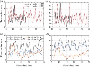


 Open access