


1. Introduction
Microplastics are a growing problem in the world's oceans. Defined as pieces of plastic less than 5 mm in size, they can have a variety of densities and shapes (Chubarenko et al. Reference Chubarenko, Bagaev, Zobkov and Esiukova2016; Law Reference Law2017). To model microplastic transport and distribution, it is necessary to understand how they are dispersed by ocean flows, and their physical characteristics (e.g. size, density and shape) are of potential importance to their dispersion. Because they can be large enough to be inertial and are typically not neutrally buoyant, they cannot be expected to behave simply as flow tracers. Particle size, for example, has been shown to impact the dispersion of spheres in turbulence (Bouvard & Petkovic Reference Bouvard and Petkovic1985). Their various shapes may further complicate their transport, as particle shape has been shown to influence how inertial particles rotate, sample the flow and settle in quiescent fluid (Willmarth, Hawk & Harvey Reference Willmarth, Hawk and Harvey1964; Auguste, Magnaudet & Fabre Reference Auguste, Magnaudet and Fabre2013; Will et al. Reference Will, Mathai, Huisman, Lohse, Sun and Krug2021), isotropic turbulence (Voth & Soldati Reference Voth and Soldati2017; Pujara, Voth & Variano Reference Pujara, Voth and Variano2019; Oehmke et al. Reference Oehmke, Bordoloi, Variano and Verhille2021) and turbulent channel flow (Zhao et al. Reference Zhao, Challabotla, Andersson and Variano2015; Shaik et al. Reference Shaik, Kuperman, Rinsky and van Hout2020; Baker & Coletti Reference Baker and Coletti2022). In quiescent fluid, discs display enhanced dispersion due to their ability to glide for long periods (Esteban, Shrimpton & Ganapathisubramani Reference Esteban, Shrimpton and Ganapathisubramani2020), and in isotropic turbulence, dispersion of rods decreases with decreasing rod length (Shin & Koch Reference Shin and Koch2005).
In the ocean, and especially at the surface or in coastal areas where microplastics are typically found (Law Reference Law2017), flows often contain both waves and currents. Waves transport particles horizontally via Stokes drift (Stokes Reference Stokes1847; Eames Reference Eames2008), which can lead to enhanced dispersion of tracers due to Taylor dispersion (Law Reference Law2000; Pearson et al. Reference Pearson, Guymer, West and Coates2002). Waves can also modify the distribution of buoyant particles, such that they congregate under wave crests (DiBenedetto Reference DiBenedetto2020), and can significantly enhance the dispersion of floating contaminants (Farazmand & Sapsis Reference Farazmand and Sapsis2019). We have previously shown numerically that variations in initial wave phase will lead to the dispersion of spherical particles (DiBenedetto, Clark & Pujara Reference DiBenedetto, Clark and Pujara2022) and that variations in initial particle orientation will lead to the dispersion of non-spherical point particles under waves (DiBenedetto, Ouellette & Koseff Reference DiBenedetto, Ouellette and Koseff2018). We have also shown that particle shape modulates the settling velocity of inertial particles (Clark et al. Reference Clark, DiBenedetto, Ouellette and Koseff2020) and that inertial non-spherical particles have a wave-preferred orientation that competes with their settling-preferred orientation (DiBenedetto & Ouellette Reference DiBenedetto and Ouellette2018; DiBenedetto, Koseff & Ouellette Reference DiBenedetto, Koseff and Ouellette2019), but there is little understanding to date of the dispersion of non-spherical particles in combined wave–current flows.
In this paper, we describe the results of laboratory experiments designed to measure the dispersion of a range of non-spherical particles in a wave–current flow. We released negatively buoyant particles of various shapes from a fixed location into a flow first with a current alone and then with both a current and waves. From their landing positions, we determined how much the particles had dispersed while they were in the flow. We found that the presence of waves significantly increased dispersion in all cases. How much the waves increased the dispersion of a particle type depended on the particle characteristics. Thinner rods and thinner discs were more dispersed by the waves than thicker rods and thicker discs, respectively, and smaller particles were more dispersed by waves than larger particles. Although the particles travelled farther under the wave scenario, the increase in their dispersion was much too large to be caused simply by increased transport distance alone. These results highlight the necessity of accounting for waves as well as particle characteristics in modelling microplastic transport in the ocean.
2. Experimental design
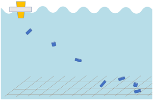
We released negatively buoyant particles of different shapes at the free surface of an open channel flow, first without waves and then again with waves (figure 1). A Buckingham Pi analysis of our experimental set-up shows that eight  $\varPi$ groups can be formed purely from the input variables because there are three dimensions (length, time and mass) and 11 independent input parameters (particle length scale $L_p$, particle eccentricity $\epsilon$, particle density $\rho _p$, fluid density $\rho _f$, dynamic viscosity $\mu$, gravity $g$, wavenumber $k$, wave amplitude $A$, mean current velocity $\bar {U}$, flow depth $H$ and flume width $b$). An example possible set of ‘input’ $\varPi$ groups is the Archimedes number $Ar$, the Stokes number $St$, the particle eccentricity $\epsilon$, the ratio between the settling time scale and the wave transport time scale $\tau _s/\tau _w$ (DiBenedetto et al. Reference DiBenedetto, Ouellette and Koseff2018), the Keulegan–Carpenter number $KC$, the wave steepness $kA$, the mean flow Reynolds number $Re$ and the wave Reynolds number $Re_w$. (See the Appendix for full definitions of these $\varPi$ groups.) With so many independent $\varPi$ groups in this system, we of course expect that dispersion will be dictated by multiple factors. In this study, we test how significantly the presence of waves affects particle dispersion and focus on how particle shape (eccentricity, which is a function of the aspect ratio) and particle size (Archimedes number $Ar=gL_p^3 \rho _f (\rho _p-\rho _f )/\mu ^2$, where $L_p^3$ is particle volume) modulate this effect. Therefore, we hold the flow-specific dimensionless groups (i.e. $kA$,
$kA$,  $Re$ and $Re_w$) constant and systematically vary particle shape and size.

Figure 1. Sketch of the experimental set-up (not to scale).
The depth-averaged background flow was approximately 5 cm s $^{-1}$ for both sets of experiments and was not turbulent. The water depth was 33.3 cm and the flume width was 31.2 cm, so the Reynolds number of the mean flow calculated based on the hydraulic radius was 5400. The flume was not inclined relative to gravity. Surface gravity waves were generated by a plunging Scotch-yoke style wavemaker. They were well described by linear wave theory, with a frequency of 1.8 Hz, amplitude of 1.4 cm, wavenumber of 13 m $^{-1}$, resulting in a wavestrength of $kA =0.18$. As indicated by these parameters and confirmed with acoustic Doppler velocimetry measurements, the waves were deep water waves, so their orbital radii decreased to a negligible $4\,\%$ ( ${\rm e}^{-{\rm \pi} }$) of the surface values at a depth of 24 cm (equivalent to half a wavelength) (Dean & Dalrymple Reference Dean and Dalrymple1991). Therefore, the particles fell out of the wavy part of the flow and ceased to be dispersed by the waves before they reached the bottom of the flume. Synthetic horsehair was placed at both ends of the flume to minimize wave reflections (figure 1), resulting in a measured reflection coefficient of 0.12 (Hughes Reference Hughes1993).
The particles were 3D-printed discs, rods and unit-aspect-ratio cylinders made from Polyamide 11 and Polyamide 12. The long axis was held constant at 7 mm for the discs and rods, while the short axis dimension had values of 1, 2 or 3 mm. One set of cylinders had a diameter (and therefore length) of 7 mm to match the long dimension of the rods and discs. There were also two smaller sets of cylinders with diameters of 3 and 4 mm, respectively, which had volumes that were more similar to those of the rods and discs. The particles had a specific gravity ranging from 1.01 to 1.04 and a measured quiescent settling velocity between 1.7 cm s $^{-1}$ (thinnest rods) and 4.7 cm s $^{-1}$ (largest cylinders). They were weakly inertial, with particle Reynolds numbers $Re_p=w_q d_p/\nu$ between 110 and 330, where $w_q$ is the quiescent settling velocity of the particle, $d_p$ is the longest length scale of the particle and $\nu$ is the kinematic viscosity of the fluid (we do not include this in our list of independent ‘input’ $\varPi$ groups because $w_q$ is a function of the other input particle and fluid parameters). We released the particles one at a time from a floating funnel tip, such that each particle entered the flow at a fixed depth of 2 cm below the local free surface in both the non-wave and wave experiments. The particles travelled downstream after being released, typically for 0.5 to 1.5 m, then landed in a catch grid at the bottom of the flume that had 1.5 cm square cells.
3. Results and discussion
For each set of flow conditions, we calculated the streamwise standard deviation of the landing positions of the particles of each type to quantify how much the particles had dispersed while they were in the flow. To quantify the additional effect of waves, we calculated the ratio between the standard deviations with waves ( $\sigma _{ww}$) and the standard deviations with no waves ( $\sigma _{nw}$). Approximately 100 particles were included in the calculation of each standard deviation ratio. Randomly subsampling one third of the data did not significantly change the standard deviation ratios, indicating that the results are converged. Since we are interested in the effects of particle shape on dispersion, we plot in figure 2 the standard deviation ratios $R_\sigma =\sigma _{ww}/\sigma _{nw}$ against the particle eccentricity, defined as $\epsilon =(\lambda ^2-1)/(\lambda ^2+1)$, where $\lambda$ is the particle aspect ratio. In this and subsequent plots, different symbols represent different particle shapes (discs, rods and cylinders), and marker sizes correspond to particle sizes (e.g. the largest asterisks represent the thickest discs, and the smallest circles represent the smallest cylinders). Error bars were computed with bootstrapping (Efron & Tibshirani Reference Efron and Tibshirani1986).

Figure 2. The standard deviation ratio  $R_\sigma =\sigma _{ww}/\sigma _{nw}$ plotted against particle eccentricity $\epsilon$, where $\sigma _{ww}$ is the standard deviation of the landing locations of the particles with waves and a current and $\sigma _{nw}$ is the standard deviation of the landing locations of the particle with a current but no waves. Blue asterisks represent discs, black circles represent cylinders with aspect ratio 1 and red triangles represent rods. Larger symbols correspond to larger particles. Error bars show $95\,\%$ confidence intervals computed with bootstrapping.
From figure 2, we see that the presence of waves increases the dispersion of the particles for all particle types except the largest cylinders. The effects can be quite dramatic: the standard deviation of the thinnest rods is increased by a factor of four when there are waves. Furthermore, the sensitivity of the particle dispersion to the presence of waves clearly changes with particle eccentricity, with thinner rods and thinner discs having a higher standard deviation ratio  $R_\sigma$ than thicker rods and thicker discs, respectively. Since the forces on particles with higher magnitudes of eccentricity vary more with different particle orientations, it is reasonable that these particles would be more dispersed by the waves. The rods also appear to be more dispersed by waves than discs or cylinders, but this may be because they have smaller volumes, as discussed subsequently. Even so, the thickest of the discs still has a standard deviation $150\,\%$ larger with waves than without waves.
We also see in figure 2 that the smaller cylinders have a higher standard deviation ratio  $R_\sigma$ than the larger cylinders, despite having the same eccentricity. This result, together with the observation that thinner rods and thinner discs have higher $R_\sigma$ values than thicker rods and thicker discs, suggests that particle size is important. To evaluate the effect of size we parameterize the particle volume using the Archimedes number (the ratio of gravitational to viscous forces), which is commonly used to categorize the dynamics of particles in flow (Tchoufag, Fabre & Magnaudet Reference Tchoufag, Fabre and Magnaudet2015; Toupoint, Ern & Roig Reference Toupoint, Ern and Roig2019; Yao, Criddle & Fringer Reference Yao, Criddle and Fringer2021). Of the parameters that contribute to the Archimedes number ( $L_p^3$, $g$,
$g$,  $\rho _p$, $\rho _f$ and $\mu$), only the particle volume $L_p^3$ varied significantly between particle types, so looking at the effect of $Ar$ for our data is essentially equivalent to looking at the effect of particle volume. Figure 3 shows the same standard deviation ratios $R_\sigma$ calculated for figure 2 but plotted against $Ar$. The horizontal error bars reflect the small variations in density amongst particles of a given type.

Figure 3. Ratio of the standard deviations of the landing locations of the particles with and without waves ( $R_\sigma =\sigma _{ww}/\sigma _{nw}$) plotted against Archimedes number $Ar$. Larger Archimedes numbers correspond to particles with larger volumes. Symbols are the same as in figure 2.
From figure 3, we can see that particles with higher  $Ar$ have smaller values of $R_\sigma$. Thus, we find that the larger a particle is, the less its dispersion is increased by the presence of waves. This result is consistent with what one might expect considering the definition of $Ar$: larger particles experience relatively stronger gravitational forces and therefore more persistently settle downward even when they are pulled in different directions by the wave effects in the flow. Larger particles are also more inertial and are therefore less perturbed by flow variations due to the presence of waves. Although there is a clear trend of larger particles dispersing less than smaller particles in waves, there is still some spread in the data, suggesting that the effects of particle volume do not supersede the effects of particle shape.
To check that the apparent impact of particle shape (as shown in figure 2) is not simply a byproduct of the effects of particle size (as shown in figure 3) or vice versa, we performed a best subsets regression analysis (Miller Reference Miller2002). To do this, we examined all possible linear regression models based on the Archimedes number  $Ar$, magnitude of the eccentricity $|\epsilon |$ and the cross-term $Ar|\epsilon |$. We use the magnitude of the eccentricity for this analysis so that higher-order terms are not required to account for the U-shape observed in figure 2. The largest cylinders are excluded from the regressions because their standard deviation ratio is unity, indicating that they are in a regime where particle volume appears to suppress all wave effects on dispersion. The results are shown in table 1. The model utilizing both $Ar$ and $|\epsilon |$ (model 4) performed far better than the model with $Ar$ alone (model 1) or the model with $|\epsilon |$ alone (model 2). While replacing $Ar$ or $|\epsilon |$ in model 4 with the cross-term (models 5 and 6) produced comparably good results, the addition of the cross-term (model 7) does not improve the adjusted $R^2$ value beyond that of model 4. These results thus indicate that it is likely that both particle shape and particle volume do indeed matter to how much particles are dispersed by waves. However, since we are able to achieve an adjusted $R^2$ value of $92\,\%$ in model 4 without accounting for the sign of the eccentricity, it is likely that discs have a lower $R_\sigma$ value than rods simply because the discs are larger than the rods. Therefore, the primary effect of particle shape is likely that particles with higher magnitudes of eccentricity are more dispersed by waves.
Table 1. Best subsets regression analysis of standard deviation ratios. Models that incorporate both the Archimedes number and the eccentricity magnitude perform far better than models which only incorporate one or the other.

Knowing that the dispersion of larger particles is less affected by the presence of waves than the dispersion of smaller particles leads us to ask whether particles disperse more when there are waves simply because the waves cause them to remain suspended in the flow longer so that they have more time to disperse. If the dispersion rate  $K=\frac {1}{2}({{\rm d}\sigma ^2}/{{\rm d}t})$ were the same whether or not waves were present, then $R_\sigma$ could be expressed as
 \begin{equation} R_\sigma=\frac{\sigma_{ww}}{\sigma_{nw}}= \frac{\sqrt{2Kt_{ww}}}{\sqrt{2Kt_{nw}}} = \left( \frac{t_{ww}}{t_{nw}} \right)^{1/2}, \end{equation}
where  $t$ represents the average time the particles spend in the flow. From (3.2) we see that enhanced dispersion could simply be caused by the particles spending more time in the flow. To check this conjecture, we consider the mean streamwise landing positions $\mu$ of the particles. The ratio between the mean landing positions of the particles with and without waves $R_\mu ={\mu _{ww}}/{\mu _{nw}}$ can then be approximated as
 \begin{equation} R_\mu=\frac{\mu_{ww}}{\mu_{nw}} \approx \frac{\overline{U_{ww}}t_{ww}}{\overline{U_{nw}}t_{nw}} = 1.1 \frac{t_{ww}}{t_{nw}}, \end{equation}
where  $\bar {U}$ is the depth-averaged velocity of the flow. When waves were present, $\bar {U}$ was approximately $10\,\%$ higher than without waves, likely due to set-up effects in the flume, which accounts for the factor of 1.1. By combining equations (3.1) and (3.2), we find that if the particles had the same dispersion rate in the flow both with and without waves, the relationship between $R_\sigma$ and $R_\mu$ would be
 \begin{equation} R_\sigma \approx ( \tfrac{1}{1.1} )^{1/2} R_\mu^{1/2}.\end{equation}
 In figure 4, we plot the standard deviation ratio  $R_\sigma$ against the mean ratio $R_\mu$ to check whether we see that relationship. We first note that the particles do indeed travel farther when waves are present: values of $R_\mu$ are greater than 1. A portion of this increased travel may be due to the small mean flow enhancement by the waves, but the rest of the increase must be due to how the particles interact with the waves. Because the direction of wave propagation is opposite that of the current, the increased particle travel is not due to Stokes drift. The standard deviation ratio $R_\sigma$ also clearly increases with the mean ratio $R_\mu$. Thus, the particles that are more dispersed by waves are indeed the same particles that travel farther when there are waves. However, if the dispersion increased simply because of this increase in the distance travelled, we would expect the data to fall on the curve representing (3.3) (the dashed curve in figure 4). Instead, the slope of the data is approximately 15 times greater. So, it is clear that although particles are transported farther by the waves, their dispersion is amplified much more significantly by the waves than can be explained solely by the increase in transport distance (time in suspension).

Figure 4. Particle standard deviation ratios  $R_\sigma = \sigma _{ww}/\sigma _{nw}$ plotted against particle mean landing location ratios $R_\mu = \mu _{ww}/\mu _{nw}$, where $\sigma$ denotes the standard deviation of the landing positions of the particles, $\mu$ denotes the mean of the landing positions of the particles, and the subscripts $ww$ and $nw$ indicate the flow cases with waves and a current and with a current but no waves, respectively. The dashed curve represents (3.3). Symbols and the meaning of the error bars are the same as in figure 2.
4. Conclusions
In summary, we find that particles disperse much more when waves are added to a current than when there is a current alone. One cause of the wave-enhanced dispersion could be variation in initial wave phase, as discussed in DiBenedetto et al. (Reference DiBenedetto, Clark and Pujara2022). Additionally, inertial discs and rods have competing settling-preferred and wave-preferred orientations (DiBenedetto et al. Reference DiBenedetto, Koseff and Ouellette2019). As particles with various initial orientations pass through different orientational trajectories to reach their settling- or wave-preferred orientations (DiBenedetto et al. Reference DiBenedetto, Ouellette and Koseff2018), they will experience differing lift and drag forces, leading to variation in their positional trajectories.
The magnitude of the wave-enhanced dispersion is dependent on particle characteristics. Thinner rods and thinner discs are more dispersed by waves than thicker rods and thicker discs, respectively, and the dispersion of larger particles is less affected by the presence of waves than the dispersion of smaller particles. Although particles that travel farther in waves are dispersed more, the increase in dispersion is too substantial to be explained by this effect alone.
These results clearly show that it is necessary to account for the presence of waves as well as particle shape and volume when modelling the transport of microplastics in the ocean. Current models often parameterize turbulent diffusion of microplastics and sometimes the vertical dispersion due to flow conditions such as breaking waves (Brunner et al. Reference Brunner, Kukulka, Proskurowski and Law2015; Kukulka & Brunner Reference Kukulka and Brunner2015), but they do not typically account for dispersion due to the interaction between waves and microplastic characteristics (Van Sebille et al. Reference Van Sebille2020). Our results also have implications for the estimation of microplastic concentrations from measurements. For example, microplastic characteristics should be accounted for when interpreting observations a certain distance from a source, as smaller microplastics will likely have spread apart more. A further unfortunate implication is that wherever there are waves, microplastics are likely to be much more difficult to remove from the ocean once they have been released since they will spread much more.
Acknowledgements
The authors are grateful to B. Sabala for assistance building the wavemaker, to H. Chung, J. Hamilton and Y. Tanimoto for help with the experimental set-up, and to N. Cowan, W. Hartog and A. Yu for helpful discussions through Stanford's Statistical Consulting service.
Funding
This work was supported by the United States National Science Foundation under grant no. CBET-1706586. L.K.C. acknowledges support from ARCS Foundation.
Declaration of interests
The authors report no conflict of interest.
Appendix
Here we define the  $\varPi$ groups that were referenced but not discussed further in the main text.
The Stokes number is the ratio between the particle response time and the characteristic flow time scale. It can be defined as  $St = ( k_\tau \rho _p d_s^2 / 18 \rho _f \nu ) / (1/\omega )$, where $d_s$ is the diameter of a volume-equivalent sphere and $k_\tau$ is a shape-dependent correction factor. Formulae for $k_\tau$ are reported in Voth & Soldati (Reference Voth and Soldati2017). However, these formulae do not always correspond well to the dynamics of non-spherical particles in wavy flows, as shown in DiBenedetto et al. (Reference DiBenedetto, Ouellette and Koseff2018). It is difficult to define $k_\tau$ for non-spherical particles because their response time varies depending on particle orientation (also see discussion in Baker & Coletti (Reference Baker and Coletti2022)). The particle response time is also generally difficult to define for finite-sized particles outside of the viscous regime, making the particle Stokes number a less useful parameter for the particles in our experiment.
The ratio between the settling time scale and the wave transport time scale can be defined as  $\tau _s/\tau _w = \omega k A^2 / w_q$, where $\omega$ is the wave frequency and is defined as $\sqrt {k g}$ for deep water waves and $w_q$ is the quiescent settling velocity of the particles, which is purely a function of particle characteristics (DiBenedetto et al. Reference DiBenedetto, Ouellette and Koseff2018). This ratio remained within a small range (between 0.2 and 0.8) for our experiments.
The Keulegan–Carpenter for a wave–current flow can be defined as  $(\omega A + U)(1/\omega )/d_s$. It expresses the ratio between the maximum fluid excursion length during a wave period and the particle length scale. It remained within a small range (between two and eight) for our experimental runs.
The wave Reynolds number is defined as  $\rho _f (\omega A) H / \mu$ and was 8300 for our experiment. It expresses the ratio between wave-induced inertia and viscosity.


 Open access