


1. Introduction
In hypersonic flight, the airflow over the fuselage of the aircraft often involves shock waves, compressible boundary layers, intense heating and significant fluctuations of temperature, velocity and pressure (Bertin & Cummings Reference Bertin and Cummings2006; Urzay Reference Urzay2018). A cornerstone of hypersonic flows is the close coupling between the kinetic and thermal energies of the gas, which leads to the development of exceedingly high temperatures in regions near the fuselage where the flow decelerates or completely stagnates. As a result, complex thermochemical processes activated by high temperatures, such as vibrational excitation and dissociation of the gas molecules, may become important near the wall (Park Reference Park1989a; Anderson Reference Anderson2006; Candler Reference Candler2019). In addition, the occurrence of transition to turbulence in hypersonic boundary layers along the fuselage is often associated with a spatially localized increase of the values of shear stress and heat flux by factors of order 10 (van Driest Reference van Driest1956; Wright & Zoby Reference Wright and Zoby1977). From an engineering standpoint, the increase in the thermomechanical loading of the wall poses challenges in the design of hypersonic vehicles by taxing the structural integrity of the fuselage. The present work employs a direct numerical simulation (DNS) of a zero-pressure-gradient hypersonic boundary layer of air over a flat, cold, isothermal, non-catalytic surface to investigate the interplay of transition and turbulence with high-enthalpy thermochemical effects.
Early computational work on high-speed boundary layers over flat plates has been mostly focused on calorically perfect gases at supersonic (Guarini et al. Reference Guarini, Moser, Shariff and Wray2000; Gatski & Erlebacher Reference Gatski and Erlebacher2002; Pirozzoli, Grasso & Gatski Reference Pirozzoli, Grasso and Gatski2004; Bernardini & Pirozzoli Reference Bernardini and Pirozzoli2011; Wenzel et al. Reference Wenzel, Selent, Kloker and Rist2018) and hypersonic (Martin Reference Martin2007; Duan, Beekman & Martin Reference Duan, Beekman and Martin2011; Franko & Lele Reference Franko and Lele2013; Fu et al. Reference Fu, Karp, Bose, Moin and Urzay2021) Mach numbers. These studies have highlighted the robustness of classic concepts for the analysis of compressible wall-bounded turbulence over near-adiabatic walls such as the Reynolds analogy, the van Driest velocity transformation (van Driest Reference van Driest1956) and the Morkovin hypothesis (Morkovin Reference Morkovin1962). In contrast, these classic concepts break down in flows subjected to significant wall cooling (Duan, Beekman & Martin Reference Duan, Beekman and Martin2010; Modesti & Pirozzoli Reference Modesti and Pirozzoli2016; Sciacovelli, Cinnella & Gloerfelt Reference Sciacovelli, Cinnella and Gloerfelt2017; Zhang, Duan & Choudhari Reference Zhang, Duan and Choudhari2018). The wall-cooled case, however, is of practical relevance for hypersonic flight, in that realistic values of the skin temperature of the fuselage at hypersonic Mach numbers (i.e. 1000–2000 K) are always small compared with the free-stream stagnation temperature. Some progress in the interpretation of the mean velocity profile of wall-bounded compressible turbulent flows has been recently made by revised transformations (Trettel & Larsson Reference Trettel and Larsson2016), which, supplemented with the semi-local scaling proposed by Huang, Coleman & Bradshaw (Reference Huang, Coleman and Bradshaw1995), have provided better collapse for compressible turbulent channel flows (Modesti & Pirozzoli Reference Modesti and Pirozzoli2016; Sciacovelli et al. Reference Sciacovelli, Cinnella and Gloerfelt2017). Data-driven techniques have also been employed for similar purposes (Volpiani et al. Reference Volpiani, Iyer, Pirozzoli and Larsson2020).
High-enthalpy effects on hypersonic flows have been mainly studied within the context of stagnation-point flows around blunt bodies (Lees Reference Lees1956; Fay & Riddell Reference Fay and Riddell1958; Liñán & Da Riva Reference Liñán and Da Riva1962; Candler & MacCormack Reference Candler and MacCormack1991; Armenise et al. Reference Armenise, Capitelli, Colonna and Gorse1996; Colonna, Bonelli & Pascazio Reference Colonna, Bonelli and Pascazio2019; Chen & Boyd Reference Chen and Boyd2020). Whereas these flows remain mostly laminar, particularly in re-entry applications because of the high altitudes, high temperatures and favourable pressure gradients involved, their thermochemical modelling requires complex descriptions that have been the focus of a number of investigations (Colonna et al. Reference Colonna, Armenise, Bruno and Capitelli2006; Panesi et al. Reference Panesi, Magin, Bourdon, Bultel and Chazot2011; Panesi & Lani Reference Panesi and Lani2013; Liu et al. Reference Liu, Panesi, Sahai and Vinokur2015). Investigations combining high enthalpies and low altitudes, where turbulence may play an important role, are much more scarce. Important studies in this field are those of Martin & Candler (Reference Martin and Candler2001) and Duan & Martin (Reference Duan and Martin2009, Reference Duan and Martin2011a), which consisted of temporally evolving boundary layers supplemented with simplified dissociation chemistry. Those studies showed that the turbulent kinetic energy is significantly altered by the chemical heat absorption, yet they did not address the spatial evolution of the boundary layer. Efforts related to the spatial evolution have been limited to laminar boundary layers (Moore Reference Moore1952; Inger Reference Inger1964) and their linear stability (Malik & Anderson Reference Malik and Anderson1991; Chang, Vinh & Malik Reference Chang, Vinh and Malik1997; Johnson, Seipp & Candler Reference Johnson, Seipp and Candler1998; Franko, MacCormack & Lele Reference Franko, MacCormack and Lele2010; Ghaffari et al. Reference Ghaffari, Marxen, Iaccarino and Shaqfeh2010). These linear-stability studies have shown that the coupling of the chemical heat absorption by dissociation within the boundary layer significantly slows down the growth of disturbances and delays transition to turbulence. These results have been confirmed by analyses using parabolized stability equations (Chang et al. Reference Chang, Vinh and Malik1997; Johnson & Candler Reference Johnson and Candler2005), and by numerical simulations precluded to the initial stages of transition (Marxen et al. Reference Marxen, Magin, Iaccarino and Shaqfeh2011, Reference Marxen, Magin, Shaqfeh and Iaccarino2013; Marxen, Iaccarino & Magin Reference Marxen, Iaccarino and Magin2014; Knisely & Zhong Reference Knisely and Zhong2019). However, none of these studies have considered the spatial evolution of a high-enthalpy hypersonic boundary layer from laminar to fully turbulent states.
In this study a statistical analysis of direct numerical simulation results of a spatially developing transitional hypersonic boundary layer at Mach 10 and sufficiently high enthalpy to induce air dissociation is presented. The rest of the paper is organized as follows. The formulation of the problem along with the computational set-up are outlined in § 2. A statistical analysis of the DNS results is presented in § 3 focusing on the streamwise evolution of wall friction and heating, along with the velocity, temperature, species concentration profiles and their cross-correlations. Concluding remarks are provided in § 4. Additionally, two appendices are included that provide a locally self-similar formulation for calculating the laminar inflow profiles (appendix A), along with a grid convergence study (appendix B). A supplementary report (Urzay & Di Renzo Reference Urzay and Di Renzo2021), devoted to hypersonic turbulent flows at suborbital enthalpies, provides additional results and schematics, including considerations about aerodynamic aspects of low-altitude hypersonic flight.
2. Formulation
This section outlines the formulation and computational set-up of the problem, including the conservation equations, boundary conditions, flow parameters and spatiotemporal resolution. In-depth details about the numerical methods, thermophysical and transport properties, and computational solver employed to address this problem can be found in Di Renzo, Fu & Urzay (Reference Di Renzo, Fu and Urzay2020).
2.1. Conservation equations
In this work, the Navier–Stokes conservation equations
 \begin{gather} {\frac{\partial {(\rho {\boldsymbol{u}})}}{\partial {t} }} + {\boldsymbol{\nabla} \boldsymbol{\cdot} } \left( \rho {\boldsymbol{u}} {\boldsymbol{u}}\right) = - \boldsymbol{\nabla} P+{\boldsymbol{\nabla} \boldsymbol{\cdot} } \bar{\bar{\boldsymbol{\tau}}}, \end{gather}
 \begin{gather}{\frac{\partial {(\rho e_0)}}{\partial {t} }} + {\boldsymbol{\nabla} \boldsymbol{\cdot} } \left( \rho e_0{\boldsymbol{u}} \right) = {\boldsymbol{\nabla} \boldsymbol{\cdot} } \left(-{\boldsymbol{u}} P + \bar{\bar{\boldsymbol{\tau}}} {\boldsymbol{u}}+\lambda \boldsymbol{\nabla} T - {\sum_{i=1}^{{N_s}}} \rho Y_i {\boldsymbol{V}}_{{\boldsymbol{i}}} h_i \right), \end{gather}
 \begin{gather}{\frac{\partial {(\rho Y_i)}}{\partial {t} }} + {\boldsymbol{\nabla} \boldsymbol{\cdot} } \left(\rho Y_i {\boldsymbol{u}}\right) = -{\boldsymbol{\nabla} \boldsymbol{\cdot} } \left(\rho Y_i{\boldsymbol{V}}_{\boldsymbol{i}} \right) + \dot{w}_{i} \quad \text{for}\ i= 1,\dots,{N_s}, \end{gather}
are integrated numerically. In this formulation,  $\{x,y,z\}$ corresponds to a Cartesian coordinate system placed adjacent to the wall, with $x$,
$x$,  $y$ and $z$ pointing, respectively, in the downstream, wall-normal and spanwise directions. In this coordinate system, the corresponding components of the flow velocity vector ${\boldsymbol {u}}$ are $\{u,v,w\}$. In addition, $t$ is the time coordinate, $\rho$ is the density, $Y_i$ is the mass fraction of species $i$ and ${{N_s}}$ is the number of species. The conservation equations are supplemented with the equation of state for a multicomponent chemically reacting mixture of ideal gases,
 \begin{equation} P= \rho {R}^{0} T/\bar{W}, \end{equation}
where  ${R}^{0}$ is the universal gas constant and $\bar {W}=(\sum _{i=1}^{N_s} Y_i/W_i)^{-1}$ is the mean molecular weight based on the individual values $W_i$ of each component.
In the momentum conservation equation (2.1), the symbol  $\bar {\bar {\boldsymbol {\tau }}}$ denotes the viscous stress tensor
 \begin{equation} \bar{\bar{\boldsymbol{\tau}}}= \mu \left[ \boldsymbol{\nabla}{\boldsymbol{u}} + \boldsymbol{\nabla}{\boldsymbol{u}}^T - 2\left( \boldsymbol{\nabla}\boldsymbol{\cdot}\boldsymbol{u}\right) \bar{\bar{\boldsymbol{I}}}/3 \right], \end{equation}
where  $\bar {\bar {\boldsymbol {I}}}$ is the identity tensor and $\mu$ is the dynamic viscosity of the mixture, the latter being evaluated using Wilke's rule based on the local dynamic viscosity of each component (Wilke Reference Wilke1950).
In the stagnation energy equation (2.2), the symbol  $e_0 = e + |{\boldsymbol {u}}|^2/2$ denotes the stagnation internal energy, with $e$ being the specific internal energy of the mixture defined as
 \begin{equation} e = h - P/\rho = {\sum_{i=1}^{{N_s}}} Y_i h_i - P/\rho, \end{equation}
where  $P$ is the thermodynamic pressure, $h$ is the specific enthalpy of the mixture and $h_i$ is the partial specific enthalpy of species $i$ given by
 \begin{equation} h_i = h_{i,{ref}}+\int_{T_{ref}}^T c_{p,i}(T')\,\textrm{d}T'. \end{equation}
In this formulation  $h_{i,{ref}}$ is a reference value of the specific enthalpy taken at the reference temperature $T_{ref}$. Similarly, $c_{p,i}$ is a temperature-dependent specific heat of species $i$ at constant pressure, which is evaluated using the nine-coefficient NASA polynomials tabulated in McBride, Zehe & Gordon (Reference McBride, Zehe and Gordon2002), which assume equilibrium in the rotational, vibrational and electronic internal degrees of freedom of the gas. The thermal conductivity of the mixture, $\lambda$, is computed by averaging the local thermal conductivities of each individual component of the mixture in accordance with the formulation described in Mathur, Tondon & Saxena (Reference Mathur, Tondon and Saxena1967).
In the species conservation equation (2.3), the diffusion velocity vector  ${\boldsymbol {V}}_{\boldsymbol {i}}$ is defined as
 \begin{equation} {\boldsymbol{V}}_{\boldsymbol{i}} = - D_i \boldsymbol{\nabla}\left( \ln X_i \right) + {\sum_{j=1}^{{N_s}}} Y_j D_j \boldsymbol{\nabla} \left( \ln X_j \right). \end{equation}
The two terms on the right-hand side of (2.8) correspond, respectively, to a Fickian flux and a mass corrector (Curtiss & Hirschfelder Reference Curtiss and Hirschfelder1949; Coffee & Heimerl Reference Coffee and Heimerl1981; Ern & Giovangigli Reference Ern and Giovangigli1994). In the notation,  $X_i$ and $D_i$ are the molar fraction and mixture-averaged mass diffusivity of species $i$, respectively. The latter is computed using the formulation in Bird, Stewart & Lightfoot (Reference Bird, Stewart and Lightfoot1960) that weighs individual binary diffusivities computed as a function of the local temperature and pressure from collision integrals based on the Stockmayer potential (Monchick & Mason Reference Monchick and Mason1961; Hirschfelder, Curtiss & Bird Reference Hirschfelder, Curtiss and Bird1964).
The chemical production rates  $\dot {w}_i$ in (2.3) are computed by considering $\textrm {N}_{2}$, $\textrm {O}_{2}$, NO, O and N as main participating species in the dissociated air, a good approximation for temperatures below 6000 K at typical post-shock pressures corresponding to stratospheric flight, where ionization effects are negligible. The expressions above should therefore be particularized for $N_s=5$. These species are produced or depleted in accordance with the five reversible chemical steps (Vincenti & Krüger Reference Vincenti and Krüger1965; Apouix Reference Apouix1989; Park Reference Park1989a,b)
 \begin{gather} \textrm{O}_2 + \textrm{M} \rightleftharpoons 2\textrm{O} + \textrm{M}, \end{gather}
 \begin{gather} \textrm{NO} + \textrm{M} \rightleftharpoons \textrm{N} + \textrm{O} + \textrm{M}, \end{gather}
 \begin{gather} \textrm{N}_{2} + \textrm{M} \rightleftharpoons 2\textrm{N} + \textrm{M}, \end{gather}
 \begin{gather} \textrm{N}_{2} + \textrm{O} \rightleftharpoons \textrm{NO} + \textrm{N}, \end{gather}
 \begin{gather} \textrm{NO} + \textrm{O} \rightleftharpoons \textrm{O}_{2} + \textrm{N}, \end{gather}
where the symbol  $\textrm {M}=\textrm {N}_{2}$, $\textrm {O}_{2}$, O, NO and N represents the third body. In the conditions analysed here, the most relevant third bodies are $\textrm {N}_{2}$, $\textrm {O}_{2}$ and O. The reactions (R1)–(R5) are endothermic in the forward direction. Dissociation or recombination processes (in the forward and backward directions, respectively) are provided by reactions (R1), (R2) and (R3). Rearrangement processes involving production of NO are described by the shuffle reactions (R4) and (R5). Specifically, (R4) in the forward direction, along with (R5) in the backward direction, correspond to the Zel'dovich mechanism of nitric-oxide production (Williams Reference Williams1985).
The rate of production of mass of species  $i$ per unit volume $\dot {w}_{i}$ participating in (2.3) can be expressed as
 \begin{equation} \dot{w}_{i} = W_i\sum_{j=\textrm{R}1}^{\textrm{R}5} (\nu''_{ij}-\nu'_{i}) \sum_{i=1}^{N_s} F_{ij} \left(\frac{\rho Y_{i}}{W_i}\right) \left[ k_{f,j} \prod_{i=1}^{N_s} \left(\frac{\rho Y_{i}}{W_i}\right)^{\nu'_{ij}} - k_{b,j} \prod_{i=1}^{N_s} \left(\frac{\rho Y_{i}}{W_i}\right)^{\nu''_{ij}} \right], \end{equation}
where  $\nu _{ij}'$ is the stoichiometric coefficient of reactant $i$ in step $j$ on the reactant side, and $\nu _{ij}''$ is the stoichiometric coefficient of reactant $i$ in step $j$ on the product side. Additionally, $F_{ij}$ is the chaperon efficiency of species $i$ participating as a third body in reaction $j$, and $k_{f,j}$ and $k_{b,j}$ are, respectively, the forward and backward rate constants of the $j$th step, which are evaluated here in terms of the equilibrium temperature $T$. Details of the chemical mechanism, including the values of $F_{ij}$ and $k_{f,j}$ for the reactions (R1)–(R5) used in this study, can be found in Park (Reference Park1989b). More complex dissociation mechanisms that account for vibrationally excited states exist in the recent literature for operating conditions warranting the consideration of thermodynamic non-equilibrium, as this topic represents an active area of research in hypersonics (Chaudhry et al. Reference Chaudhry, Boyd, Torres, Schwartzentruber and Candler2020; Finch et al. Reference Finch, Girard, Strand, Yu, Austin, Hornung and Hanson2020; Streicher et al. Reference Streicher, Krish, Hanson, Hanquist, Chaudhry and Boyd2020).
2.2. Flow parameters and computational set-up
The problem addressed in this study is a nominally zero-pressure-gradient transitional boundary layer flow at an edge Mach number  $Ma_e = U_e / a_e = 10$ based on the edge values of the velocity $U_e$ and frozen speed of sound $a_e$. The edge values of pressure and temperature are $P_e = {57.1}\ \textrm {kPa}$ and $T_e = 1039\ \textrm {K}$, respectively. These conditions approximately resemble those of a chemically frozen and thermodynamically equilibrated post-shock inviscid airflow (with edge mass fractions $Y_{{\textrm {N}_{2}},e}=0.767$ and $Y_{{\textrm {O}_{2}},e}=0.233$) downstream of an oblique shock wave generated by a planar wedge of semi-angle $9^{\circ }$ flying at Mach 23 at 25 km of altitude in the stratosphere. Note that the quantities $U_e$, $Y_{{\textrm {N}_{2}},e}$, $Y_{{\textrm {O}_{2}},e}$, $P_e$ and $T_e$, along with the edge density $\rho _e$ and edge static enthalpy $h_e$ used below, correspond to values in the free stream overriding the laminar boundary layer near the inflow, where edge conditions are unequivocally defined, and where the boundary layer has not yet been disturbed by the method employed to induce transition (i.e. see § 2.3 for further details). It should however be emphasized that $U_e$, $Y_{{\textrm {N}_{2}},e}$, $Y_{{\textrm {O}_{2}},e}$, $T_e$ and $h_e$ undergo negligible changes along the free stream, whereas $\rho _e$ and $P_e$ vary by approximately 10 % as a result of an acoustic wave generated by the method employed to induce transition, as described in § 3.4.
The value of the stagnation enthalpy at the edge of the boundary layer,  $h_{0,e} = h_{e} + U_e^2/2= 21.6\ \textrm {MJ}\ \textrm {kg}^{-1}$, is approximately 80 % of kinetic origin. In particular, $h_{0,e}$ is smaller than the dissociation energy of $\textrm {N}_{2}$, $36.6\ \textrm {MJ}\ \textrm {kg}^{-1}$, but larger than the dissociation energy of $\textrm {O}_{2}$, approximately $15.5\ \textrm {MJ}\ \textrm {kg}^{-1}$. In addition, $h_{0,e}$ is much larger than the characteristic vibrational energies of $\textrm {N}_{2}$ and $\textrm {O}_{2}$, which approximately correspond, respectively, to $1.0\ \textrm {MJ}\ \textrm {kg}^{-1}$ and $0.6\ \textrm {MJ}\ \textrm {kg}^{-1}$. As a result, and despite the fact that not all the free-stream kinetic energy is transformed into static enthalpy as the flow decelerates near the wall, the aforementioned operating conditions warrant that the flow there attains thermal enthalpies leading to dissociation of $\textrm {O}_2$, production of NO and significant vibrational excitation of both $\textrm {N}_2$ and $\textrm {O}_{2}$. In contrast, as indicated by the results presented below, the $\textrm {N}_{2}$ molecules do not dissociate as much, thereby leading to relatively small concentrations of atomic nitrogen in the boundary layer.
The entire surface of the plate is considered to be isothermal at a temperature  $T_w = 1700\ \textrm {K}$, which amounts to approximately 10 % of the edge stagnation temperature $T_{0,e}$ had the overriding gas been assumed to be calorically perfect, $T_w/T_{0,e}=0.07$. It is shown below that the temperature profile develops a maximum in both the laminar and turbulent portions of the boundary layer, in a manner similar to that observed in simulations of calorically perfect gases over cold walls, $T_w/T_{0,e} < 1$. The resulting non-monotonicity in the temperature profile is caused by viscous aerodynamic heating, which is responsible for transferring heat from the gas within the boundary layer to the plate. In addition, the wall is assumed to be non-catalytic, in such a way that the wall-normal diffusion velocity (2.8) vanishes at the surface for all species, or equivalently, ${\partial Y_i}/{\partial y} \vert _{w} = 0$ for $i=1,2,\dots N_s$. A consequence of this approximation is that the heat otherwise released within catalytic walls by recombination reactions is zero in the present simulations.
The computational domain is a cuboid adjacent to the surface of the plate and aligned with the free-stream velocity vector. The boundary layer entering the computational domain through its upstream boundary at  $x=x_o=65\delta ^*_o$ is laminar at a Reynolds number $Re_{\delta ^*_o}=\rho _e U_e \delta ^*_o /\mu _e=6000$, where $\delta ^*_o$ is the local displacement thickness, and $\rho _e$ and $\mu _e$ are the edge values of the density and molecular viscosity, respectively. The profiles of temperature, velocity and mass fraction of the inflow boundary layer are determined by solving the locally self-similar form of the laminar boundary-layer equations outlined in appendix A. Based on the inflow streamwise location and the inflow displacement thickness, a dimensionless streamwise coordinate can be defined as
 \begin{equation} \hat{x}=(x-x_o)/\delta^{\star}_o, \end{equation}
which is used below for data analysis.
The dimensions of the computational domain are  $1800\delta _o^\star \times 75\delta _o^\star \times 20{\rm \pi} \delta _o^\star$ in the streamwise, wall-normal and spanwise direction, respectively. The computational domain is discretized using $11\,648 \times 350 \times 512$ grid points along the same directions (i.e. approximately 2.1 billion grid points). The grid points in the $x$- and $z$-directions are uniformly distributed, whereas the stretching function $y_j = 75 \delta _o^\star \{ \sinh { (s j/350 ) } + \sinh { [s (j-1) /350 ] } \}/[2 \sinh {(s)}]$, with $s = 5.1$ and $j = 1, 2, \dots , 350$, is used to warrant higher wall-normal resolution near the wall and ensure that the size $\Delta y^+_w$ of the first cell next to the wall is smaller than unity everywhere, as shown in table 1. In this notation, the superscript $+$ is used to denote normalization with the viscous length scale $\overline {\mu _w}/( \overline {\rho _{w}} u_{\tau } )$, where $\overline {\mu _w}$ and $\overline {\rho _w}$ are time- and spanwise-averaged values of the molecular viscosity and density at the wall, and $u_{\tau } = \sqrt {\overline {\tau _w}/\overline {\rho _w}}$ is the friction velocity based on the time- and spanwise-averaged wall shear stress $\tau _w$. A grid-refinement study is presented in appendix B that shows the appropriateness of this resolution for the present configuration.
Table 1. Time- and spanwise-averaged dimensionless quantities computed at the dimensionless streamwise locations indicated in the first row. In the notation,  $Re_x = \rho _e U_e x/\mu _e$ is the Reynolds number based on the streamwise distance $x$ measured from the leading edge of the plate, $Re_\tau = \overline {\rho _w} u_{\tau } \delta _{99}/\overline {\mu _w}$ is the friction Reynolds number based on the local boundary-layer thickness $\delta _{99}$ and $Re_{\delta ^*} = \rho _e U_e \delta ^*/\mu _e$ is the Reynolds number based on the local displacement thickness $\delta ^*$. In addition, $Re_\theta = \rho _e U_e \theta /\mu _e$ and $Re_{\theta ,w} = \overline {\rho _w} U_e \theta /\overline {\mu _w}$ are momentum Reynolds numbers based on the local momentum thickness $\theta$ and on edge or wall properties. The symbol $Ma_\tau = u_\tau /\overline {a_w}$ denotes the friction Mach number, $H = \delta ^*/\theta$ represents the boundary-layer shape factor and $B_q = \overline {q_w}/( \overline {\rho _w} u_\tau \overline {h_w} )$ is the dimensionless heat flux at the wall based on the averaged enthalpy at the wall $\overline {h_w}$. The remaining symbols $\Delta x^+$, $\Delta z^+$, $\Delta y_w^+$ and $\Delta y_{99}^+$ indicate the grid size in local viscous units in the $x$-direction, in the $z$-direction, in the $y$-direction at the wall $y=0$ and in the $y$-direction at $y=\delta _{99}$ away from the wall, respectively.

One-dimensional non-reflecting boundary conditions (Poinsot & Lele Reference Poinsot and Lele1992; Okong'o & Bellan Reference Okong'o and Bellan2002) are imposed at the inflow boundary  $x=x_o$ (i.e. $\hat {x}=0$), at the outflow boundary $x=x_o+ 1800\delta _o^\star$ (i.e. $\hat {x}=1800$) and along the upper surface of the cuboidal domain $y = 75 \delta _o^\star$. Specifically, the value of the pressure is weakly imposed on the zones of these boundaries where the local outflow normal velocity is subsonic. The non-slip velocity condition is imposed on the surface of the plate $y = 0$, except for a narrow strip where a suction-and-blowing boundary condition is imposed for the wall-normal velocity to trigger transition in the laminar boundary layer, as described below.
The gas is assumed to be in vibrational equilibrium everywhere. A number of cautionary remarks must be made with regards to this approximation. In the free stream, where the temperature  $T_e$ is relatively low, the contribution of the vibrational degrees of freedom to the internal energy is small, and, therefore, the approximation of vibrational equilibrium has a negligible effect. Within the boundary layer, however, high temperatures of approximately $T_{{max}}\approx 4T_e$ develop as a result of aerodynamic heating that profusely activate the vibrational degrees of freedom. There, the values of the characteristic vibrational relaxation time scale $t_v$ for $\textrm {N}_{2}$ and $\textrm {O}_{2}$ molecules are, respectively, 12 times and 1.4 times larger than the flow residence time $x_o/U_e$ of the gas within the boundary layer entering the computational domain (see p. 58 in Park (Reference Park1989a) for details of the calculation of $t_v$). This suggests that the gas molecules are not strictly in vibrational equilibrium at the inflow. In contrast, at the outflow of the computational domain, the flow residence time is approximately larger than $x_o/U_e$ by a factor of 30, thereby leaving room for the vibrational relaxation of the gas molecules as they are transported by the mean flow along the plate. In addition, a complicating factor in the turbulent portion of the boundary layer is that sweeps and ejections mix hot gases near the wall with cold gases near the edge, and may, in principle, lead to lags in the vibrational energy with respect to its thermodynamic-equilibrium value. The structures responsible for this mixing are large-scale ones that turn in time scales of the same order as the displacement thickness divided by the friction velocity, which, in the present operating conditions, are slower than $t_v$ by a factor of 13 for $\textrm {O}_{2}$, but faster than $t_v$ by a factor of 1.3 for $\textrm {N}_{2}$. In this way, whereas the $\textrm {O}_{2}$ molecules may vibrationally equilibrate promptly when overturned by these large eddies, the $\textrm {N}_{2}$ molecules may remain vibrationally frozen (during sweeps) or vibrationally equilibrated (during ejections), thereby complicating the description. As shown below, the dissociation of $\textrm {N}_{2}$ is negligible, and, therefore, the effect of the vibrational non-equilibrium of the $\textrm {N}_{2}$ molecules in the conditions studied here is restricted to modifying the thermal inertia of the gas. On the other hand, the approximation of vibrational equilibrium for $\textrm {O}_{2}$ may overestimate the rate of the dissociation step (R1) forward, which is responsible for activating the shuffle reactions (R4) forward and (R5) backward. These estimates suggest that the consideration of vibrational non-equilibrium represents a relevant aspect worthy of future work aiming at improving the present analysis. Additional considerations about thermodynamic non-equilibrium effects on hypersonic turbulent boundary layers are provided in Urzay & Di Renzo (Reference Urzay and Di Renzo2021).
2.3. Method for inducing transition
Using an approach similar to that proposed by Franko & Lele (Reference Franko and Lele2013), the transition of the laminar boundary layer is induced by means of a suction-and-blowing boundary condition that is imposed on the region of the surface of the plate  $y=0$ lying within the strip $15\delta _{o}^{*} \leqslant x - x_o \leqslant 20\delta _{o}^{*}$, There, the non-penetration boundary condition for the wall-normal velocity component $v=0$ is replaced by the travelling wave $v= f(x) g(z) \sum _{i=1}^{10} A_i \sin (\omega _i t - \beta _i z)$. In this formulation, the function $f(x) = \exp [-(x/\delta _{o}^{*} - x_s/\delta _{o}^{*})^2/(2\sigma ^2)]$ forces a Gaussian-like distribution of $v$ across the streamwise width of the strip, with $x_s = 17.5\delta _{o}^{*}$ and $\sigma = 0.75$. In addition, the function $g(z) = 1.0 + 0.1 \{ \exp \{-[(z - z_c - z_w)/z_w]^2\} + \exp \{-[(z - z_c + z_w)/z_w]^2\}\}$, with $z_c = 10 {\rm \pi}\delta _{o}^{*}$ and $z_w = 2 {\rm \pi}\delta _{o}^{*}$, is utilized to break the symmetry of the disturbance in the spanwise direction by adding a small-amplitude stationary distortion. The chemical composition of the fluid injected or bled by this boundary condition is imposed in such a way that it satisfies the non-catalytic boundary condition mentioned above.
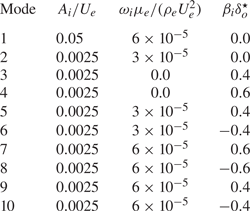
Transition is induced by injecting the modes provided in table 2 and defined by their dimensionless amplitudes  $A_i/U_{e}$, frequencies $\omega _i \mu _{e} / ( \rho _{e} U_{e}^2 )$ and spanwise wavenumbers $\beta _i \delta _o^\star$. The primary wave forced in the flow, corresponding to mode 1 in table 2, is mostly two dimensional (up to the small spanwise non-uniformity introduced by $g(z)$) and resembles a second Mack mode in classic terminology for boundary-layer transition of calorically perfect gases (Mack Reference Mack1969). The remaining modes contain three-dimensional (3-D) waves with non-zero wavenumbers and much smaller amplitudes imposed by resemblance with Franko & Lele (Reference Franko and Lele2013). The frequency of the primary wave is equivalent to a dimensional linear frequency $f_1=\omega _1/2{\rm \pi} =1730$ kHz, and was determined in auxiliary simulations by maximizing the energy growth in a purely two-dimensional (2-D) laminar boundary layer computed at the same operating conditions as those described above. The resulting wavelength of the primary wave in viscous units immediately downstream of the aforecited injection strip at $x-x_o = 22\delta _0^\star$ is $\overline {\rho _w}A_1 u_{\tau }/(\,f_1\overline {\mu _w})=43$, which corresponds to 66 times the local grid spacing in the $y$-direction at that location, thereby ensuring proper resolution of the ensuing wave.
Table 2. Dimensionless amplitude, frequency and spanwise wavenumber of the modes excited by the suction-and-blowing boundary condition.
2.4. Numerical methods and data-sampling rates
The formulation described above is discretized on a stretched collocated Cartesian grid using the sixth-order low-dissipation TENO6-A scheme outlined in Fu (Reference Fu2019), which is designed to recover a sixth-order central finite-difference scheme for the Euler fluxes in the smooth regions of the flow, along with a second-order finite-difference central scheme for the diffusion fluxes. The conservation equations are advanced in time using the strong-stability-preserving third-order Runge–Kutta scheme described in Gottlieb, Shu & Tadmor (Reference Gottlieb, Shu and Tadmor2001) while keeping the Courant–Friedrichs–Lewy number equal to 0.8. The resulting set of algebraic equations is implemented and solved by the hypersonics task-based research (HTR) solver (Di Renzo et al. Reference Di Renzo, Fu and Urzay2020). The HTR solver leverages the runtime Legion (Bauer et al. Reference Bauer, Treichler, Slaughter and Aiken2012, Reference Bauer, Treichler, Slaughter and Aiken2014) and the programming language Regent (Slaughter et al. Reference Slaughter, Lee, Treichler, Bauer and Aiken2015) to perform the calculations efficiently on high-performance supercomputers with heterogeneous architectures consisting of CPUs and GPUs, without the need of rewriting code upon switching between these technologies. Specifically, the present simulations were performed in the heterogeneous supercomputer Lassen at the Lawrence Livermore National Laboratory. Further details of the formulation such as thermophysical and transport properties, numerical methods and computational aspects of the HTR solver are provided in Di Renzo et al. (Reference Di Renzo, Fu and Urzay2020), along with an extensive set of verification tests that includes a transitional hypersonic boundary layer.
The results presented below are obtained by time- and spanwise-averaging DNS solution snapshots of the flow field in the statistically steady state. In particular, the averages are performed by sampling the flow field every 10 time steps for about one half of the computational flow-through time. This sampling time interval is equivalent to approximately 50 periods of the first mode injected by the suction-and-blowing boundary condition and is observed to be sufficiently long to achieve adequate statistical convergence of the results. The time- and spanwise-averaged value of any variable  $\phi$ is represented by the overline symbol $\bar {\phi }$, whereas $\phi '=\phi -\bar {\phi }$ denotes the corresponding fluctuations. Similarly, density-weighted or Favre averages are denoted by the tilde symbol $\tilde {\phi }$, with $\phi ''=\phi -\tilde {\phi }$ being the fluctuations around the average.
The statistical analysis of the numerical solution is performed at the six streamwise locations indicated in table 1, which provides the corresponding local values of relevant non-dimensional integral quantities, including the local momentum-based and friction Reynolds numbers. The first location at  $\hat {x} = 400$ corresponds to conditions immediately upstream of where resonance of the 2-D mode begins. The second location at $\hat {x} = 700$ is in the region dominated by the growth of the secondary instability. The third location $\hat {x} = 1000$ represents conditions immediately upstream of where breakdown to turbulence begins. The fourth location $\hat {x} = 1300$ is near the end of the transitional region. The last two locations, $\hat {x} = 1600$ and $1750$, are embedded within the turbulent portion of the boundary layer.
3. Results
This section presents a detailed statistical analysis of the numerical solution. Particular emphasis is made on friction and wall heating, and on the distributions of main aerothermochemical variables and their evolution with distance downstream.
3.1. Friction and wall heating
The results shown below make use of the skin friction coefficient
 \begin{equation} C_f = 2\overline{\tau_w}/\left( \rho_e U_e^2\right),\end{equation}
and the dimensionless wall heat flux
 \begin{equation} C_q=\overline{q_w}/\left( \rho_e U_e^3\right). \end{equation}
In (3.2), the wall heat flux has been normalized following White (Reference White1992) with twice the flux of kinetic energy in the free stream. In contrast, the flux of enthalpy difference between the adiabatic wall enthalpy and the wall enthalpy, used for defining the traditional Stanton number, is not a constant in this problem because of the variations of chemical composition along the wall. As a result, the simultaneous variation of the numerator and denominator of the Stanton number makes this quantity a cumbersome one to interpret at the present enthalpy levels.
For  $0\leqslant \hat {x}\lesssim 15$, very close to the inflow and upstream of the wall injection strip, the boundary layer is undisturbed and, therefore, evolves as a steady two-dimensionally laminar one. A comparison is provided in the inset in figure 1(a) between the DNS distributions of $C_f$ and $C_q$ in that region and the solution obtained from the locally self-similar, laminar boundary-layer equations outlined in appendix A. An expanded version of that inset is provided in figure 14 in appendix A over a much longer streamwise region for verification purposes, where the distributions of $C_f$ and $C_q$ obtained from a full 2-D numerical simulation of the same Mach-10 undisturbed boundary layer are compared against the locally self-similar solution (see also the verification exercise for a Mach-6 laminar boundary layer provided in figure 7 in Di Renzo et al. Reference Di Renzo, Fu and Urzay2020). Perfect agreement between the locally self-similar theory and the DNS or full 2-D numerical simulations is not expected, since the theory is known to underperform because it is based on the assumption of uniform pressure across the boundary layer, which becomes an increasingly less accurate assumption as the Mach number increases (Anderson Reference Anderson2006).

Figure 1. (a) Skin friction coefficient and dimensionless wall heat flux, along with (b) molar fractions of atomic oxygen and nitric oxide at the wall. Included in the figure are DNS results (solid lines) and the solution obtained by numerically integrating the locally self-similar formulation provided in appendix A (symbols).
Near the injection strip,  $15\lesssim \hat {x}\lesssim 20$, the suction-and-blowing boundary condition creates rapid oscillations in $C_f$ and $C_q$ and leads to offsets downstream between the DNS and the laminar solution. These offsets are compounded by the normalization chosen in (3.1) and (3.2) based on the inflow edge density $\rho _e$, since the suction-and-blowing boundary condition causes a decrease in the local edge density of approximately 10 %, as described in § 3.4.
For  $20 \lesssim \hat {x} \lesssim 400$, the DNS distributions of $C_f$ and $C_q$ exhibit a laminar-like behaviour that scales approximately as $x^{-1/2}$. Significant spikes in $C_f$ and $C_q$ are observed near $\hat {x}\simeq 500$, where resonance of the 2-D mode forced with the suction-and-blowing boundary condition occurs. This resonance does not directly lead to transition, as suggested by the isosurfaces of the second invariant of the velocity-gradient tensor shown in figure 2(a), and by the streamwise velocity contours shown in the upper panel in figure 2(b). Instead, the resonance triggers a secondary instability based on the interaction of the high-order 3-D modes also seeded by the suction-and-blowing boundary condition (see table 2). Downstream of this resonance, where the secondary instability develops, $C_f$ and $C_q$ return to laminar-like distributions. At approximately $\hat {x} \simeq 1000$, the secondary instability excited by the resonance leads to breakdown, as shown in the middle panel in figure 2(b). This process is accompanied by an increase of both $C_f$ and $C_q$ by factors of approximately $4$ and $5$, respectively. Transition to turbulence is completed at approximately $\hat {x} \simeq 1500$, where turbulent flow is observed along the entire span of the domain, as shown in the lower panel in figure 2(b).

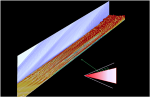
Figure 2. (a) Instantaneous visualization of the isosurfaces of the second ( $Q$) invariant of the velocity-gradient tensor coloured by the molar fraction of atomic oxygen. The side plane is coloured by the magnitude of the density gradient normalized by its maximum value. (b) Instantaneous contours of the normalized streamwise velocity on the wall-parallel plane $y = 3\delta _o^{\star }$.
Qualitatively similar transitional processes as those described above have been observed by Franko & Lele (Reference Franko and Lele2013) and Hader & Fasel (Reference Hader and Fasel2019), albeit at much lower enthalpies, at which the gas behaves as calorically perfect. It is worth mentioning that, similarly to the results in Franko & Lele (Reference Franko and Lele2013), no clear overshoot in  $C_f$ is observed downstream of the main upwards ramp in figure 1(a).
3.2. Chemical composition along the wall
The molar fractions of the major dissociation products evaluated at the wall, namely  $X_{\textrm {O},w}$ and $X_{\textrm {NO},w}$, remain small but tend to increase with distance downstream until $\hat {x}\simeq 1300$, beyond which they appear to first plunge and then plateau at approximately $6\,\%$ (for O) and $2\,\%$ (for NO), as shown in figure 1(b). The starting point of the plateaus at $\hat {x}\simeq 1400$ approximately coincides spatially with the onset of turbulence in the boundary layer, a phenomenon that is analysed later in § 3.4.
It is worth stressing that the free-stream and wall temperatures employed in these simulations are too low for sustaining any significant concentration of dissociation products near chemical equilibrium. As shown in § 3.4, the concentrations of all minor species are negligible in the free stream, where the flow remains chemically frozen. In contrast, despite the relatively low wall temperature, figure 1(b) indicates the presence of super-equilibrium concentrations of O and NO along the wall, thereby suggesting that significant dissociation has taken place somewhere within the boundary layer and some of the dissociation products have been transported to the wall by diffusion and convection. That chemical dissociation occurs within this boundary layer will be found below to be caused by the local temperature increase of the gas as a result of aerodynamic heating.
As shown in figure 1(b), the agreement between the DNS wall concentration values and the laminar solution is rapidly broken by the suction-and-blowing boundary condition imposed at the wall. As discussed more in detail in § 3.5, the perturbations induced by this boundary condition decrease the mean chemical production rates in the DNS, thereby leading to smaller concentrations of dissociated species in the mixture relative to the laminar solution.
3.3. Velocity, pressure and turbulent-Mach-number statistics
Transformed versions of the wall-normal profiles of the mean streamwise velocity using the transformations proposed by van Driest (Reference van Driest1956) and Trettel & Larsson (Reference Trettel and Larsson2016) are shown in figure 3. The profiles are plotted at the averaging statations indicated in table 1 against the wall-normal distance scaled in friction units  $\overline {\mu _w}/[\overline {\rho _w}(\overline {\tau _{w}}/\overline {\rho _w})^{1/2}]$ for $y^+$, and in semi-local units $\bar {\mu }/[\bar {\rho }(\overline {\tau _{w}}/\bar {\rho })^{1/2}]$ for $y^\star$, the latter being of relevance for compressible turbulent boundary layers subjected to significant density variations near the wall as a consequence of wall cooling (Huang et al. Reference Huang, Coleman and Bradshaw1995). The first three averaging stations $\hat {x}=400$, $700$ and $1000$ provide laminar mean velocity profiles that collapse well using the transformation proposed by Trettel & Larsson (Reference Trettel and Larsson2016), which follows better the linear scaling in the viscous sublayer. The two last averaging stations $\hat {x}=1600$ and $1750$ provide turbulent mean velocity profiles that collapse reasonably well on the incompressible log law using either transformation up to a dimensionless distance from the wall (evaluated in friction or semi-local units depending on the transformation) equal to about 200. Beyond that, significant discrepancies are observed between either one of the transformed velocities and the incompressible log law. Specifically, the transformation proposed by Trettel & Larsson (Reference Trettel and Larsson2016) leads to larger slopes in the log layer, an observation similar to that made by Zhang et al. (Reference Zhang, Duan and Choudhari2018) for wall-cooled hypersonic boundary layers of calorically perfect gases. A profile intermediate to the laminar and turbulent ones is obtained at the transitional stage $\hat {x}=1300$ that does not show evidence of any clearly layered structure with any of the two transformations.

Figure 3. Transformed mean streamwise velocity profiles using the transforms proposed by (a) van Driest (Reference van Driest1956) and (b) Trettel & Larsson (Reference Trettel and Larsson2016). Also included are the incompressible profiles in the viscous sublayer (dash double-dotted lines) and log layer (dashed lines).
Although the velocity profiles shown in figure 3 suggest that the flow at  $\hat {x} = 400$, $700$ and $1000$ is laminar on average, the boundary layer in those locations is already subjected to fluctuations induced by the suction-and-blowing boundary condition. This is revealed quantitatively by the normal components of the Reynolds stress tensor provided in figure 4(a–d). At $\hat {x} = 400$, the components $\overline {\rho u'' u''}$ and $\overline {\rho v'' v''}$ attain peak values at $y^* \simeq 10$ that are comparable to the local mean wall shear stress $\overline {\tau _w}$. In contrast, the spanwise $\overline {\rho w'' w''}$ and shear $\overline {\rho u'' v''}$ components are much smaller at that same location, as shown in figure 4(c,d). These considerations suggest that the aforementioned stress field is due to the 2-D mode forced with the suction-and-blowing boundary condition. The resonance of this mode is imminent at this streamwise location and leads to a relatively high turbulent Mach number $Ma_t\simeq 0.3$, as observed in figure 4(e), with $Ma_t$ being defined as
 \begin{equation} Ma_t=\sqrt{\overline{{\boldsymbol{u}}' \cdot {\boldsymbol{u}}'}} / \bar{a} \end{equation}
based on the local Reynolds-averaged speed of sound  $\bar {a}$.

Figure 4. Normal components of the Reynolds stress tensor in the (a) streamwise, (b) wall-normal and (c) spanwise directions, along with (d) Reynolds shear stress, (e) turbulent Mach number and (f) r.m.s. of the pressure fluctuations. The dots on the curves in panel (f) indicate the position of the edge of the boundary layer calculated as  $y=\delta _{99}$.
At  $\hat {x} = 700$, the 2-D mode has undergone resonance and is therefore subject to the secondary instability, which leads to the emergence of fully 3-D fluctuations in the laminar boundary layer. Specifically, the presence of excited 3-D modes derived from the resonance is elicited by the isotropization of the wall-normal and spanwise components of the Reynolds stress tensor in figure 4(b,c). In addition, large values in the streamwise component of the Reynolds stress tensor are attained because of the low-speed streaky structures observed in the middle panel in figure 2(b), which are positioned in between the vortices visualized in figure 2(a).
The profiles extracted at  $\hat {x} = 1000$, which is located just before the beginning of breakdown to turbulence, are similar to those at $\hat {x} = 700$ except for the generally larger values observed in the three components of the velocity fluctuations. As the flow further progresses into the breakdown stage corresponding to the main upwards ramp in the profiles of both $C_f$ and $C_q$, a large increase is observed in the maximum values of all the components of the Reynolds stress tensor, whose distributions become wider across the entire boundary layer, as shown in figure 4(a–d) for $\hat {x} = 1300$. The highest compressibility conditions are attained upon breakdown, as indicated by the large increase in the turbulent Mach number in figure 4(e) for $\hat {x} = 1300$, which peaks at a near-sonic value $Ma_t \simeq 1$ at $y^* \simeq 20$. Relative to the streamwise station near breakdown at $\hat {x} = 1300$, the attainment of fully turbulent conditions in the boundary layer at the last two streamwise stations $\hat {x} = 1600$ and $\hat {x} = 1750$ entails decrements of approximately 20 %, 50 % and 15 % in the peak values of the turbulent Mach number and the streamwise and shear components of the Reynolds stress tensor, respectively, along with an increment of approximately 15 % in the peak values of both the spanwise and wall-normal components of the Reynolds stress tensor.
The attainment of asymptotic self-similarity in turbulent boundary layers is traditionally a subject of debate at high Mach numbers, and is perhaps even more debatable in the present problem, in which air dissociation incorporates additional external time scales. Note that even the early undisturbed portion of the laminar boundary is only locally self-similar, as discussed in appendix A. However, reasonable self-similarity is observed in figure 4 between the profiles extracted at  $\hat {x} = 1600$ and $1750$, in that the Reynolds stresses appear to collapse reasonably in inner units, although it should be taken into account that the relative change in $Re_{\tau }$ in between those two streamwise stations is only moderate and approximately equal to 15 %.
The root-mean-square (r.m.s.) of the fluctuations of static pressure generally decay away from the wall, as observed in figure 4(f). However, as also noticed in Zhang et al. (Reference Zhang, Duan and Choudhari2018) for hypersonic boundary layers of calorically perfect gases, the trend here is non-monotonic with the wall-normal distance. The maximum value of the wall pressure r.m.s. is reached near resonance,  $\hat {x} \simeq 400$, and is approximately equal to 12 times the mean wall shear stress $\overline {\tau _w}$, or equivalently, to 0.5 % of the dynamic pressure $\rho _eU_e^2/2$. At the wall, in the turbulent portion of the boundary layer, the pressure fluctuations are influenced by the near-wall turbulent intensities, which are known to be higher for increasingly colder walls (Zhang et al. Reference Zhang, Duan and Choudhari2018). In comparison with early work using calorically perfect gases, the present simulations return r.m.s. values of the wall pressure within the range $5.0\overline {\tau _w}\text {--}5.5\overline {\tau _w}$ in the turbulent portion of the boundary layer, which correspond to approximately twice the values observed in Duan, Choudhari & Zhang (Reference Duan, Choudhari and Zhang2016) for Mach-2.5 adiabatic and Mach-6 slightly cooled ( $T_w/T_{a,w}=0.76$) cases, approximately 1.5 times the values reported in Zhang, Duan & Choudhari (Reference Zhang, Duan and Choudhari2017) for a Mach-6 cooled ( $T_w/T_{a,w}=0.25$) case, and similar or slightly larger than that reported in Zhang et al. (Reference Zhang, Duan and Choudhari2017) for a Mach-14 cooled ( $T_w/T_{a,w}=0.18$) case, with $T_{a,w}$ the adiabatic wall temperature. These considerations suggest that the wall pressure fluctuations in hypersonic turbulent boundary layers increase with wall cooling, and that this trend persists as the stagnation enthalpy is increased.
Near the edge of the boundary layer, upon breakdown and within the turbulent portion, the acoustic waves radiated from the boundary layer lead to r.m.s. values of the static pressure fluctuations within the range  $1.6\overline {\tau _w} \text {--}2.0\overline {\tau _w}$. Relative to the aforecited studies using calorically perfect gases, these values correspond to approximately four times the values observed in Duan et al. (Reference Duan, Choudhari and Zhang2016) for Mach-2.5 adiabatic and Mach-6 slightly cooled ( $T_w/T_{a,w}=0.76$) cases, and approximately twice the values reported in Zhang, Duan & Choudhari (Reference Zhang, Duan and Choudhari2016) and Zhang et al. (Reference Zhang, Duan and Choudhari2017) for Mach-6 cooled ( $T_w/T_{a,w}=0.25$) and Mach-14 cooled ( $T_w/T_{a,w}=0.18$) cases. Note, however, that the present r.m.s. values of the static pressure throughout the boundary layer agree better with those reported in the simulations of high-enthalpy temporally evolving boundary layers reported in Duan & Martin (Reference Duan and Martin2011a) for their $8^\circ$-wedge case, which is characterized by a similar Mach number and wall-to-stagnation temperature ratio as those used here. In particular, the present results corroborate their findings that thermochemical effects tend to increase the r.m.s. of the pressure fluctuations, including the noise radiated from the boundary layer. In view of these results, closer analyses of the fundamental mechanisms whereby thermochemical effects augment noise radiation from hypersonic boundary layers may be worthy of future investigations.
3.4. Temperature and density statistics
A non-monotonic trend in the wall-normal profile of the mean temperature can be observed in figure 5(a) that is due to the effect of aerodynamic heating in the presence of the cold wall. As the laminar boundary layer grows for  $\hat {x} \leqslant 1000$, the magnitude of the temperature peak decreases slightly and moves away from the wall in absolute units, thereby leading to the decrease in the dimensionless heat flux observed in figure 1(a). As the boundary layer transitions to turbulence near $\hat {x} =1300$, the peak temperature decreases further but the entire profile widens because of the enhanced turbulent transport. This phenomenon translates into the upwards ramp in the dimensionless heat flux shown in figure 1(a). In the turbulent portion of the boundary layer, the temperature profile becomes even wider, and the location of the peak of the temperature sits relatively close to the wall at $y^*\simeq 10$, near the wall-normal location where the peaks of streamwise normal Reynolds stress and turbulent Mach number are attained. The two farthest downstream profiles of temperature, corresponding to $\hat {x} = 1600$ and $1750$ within the turbulent region, appear to collapse reasonably well in inner units for $y^* \lesssim 100$.

Figure 5. Wall-normal profiles of (a) Favre mean temperature, (b) r.m.s. of Favre fluctuations of temperature, (c) Reynolds mean density (d) and r.m.s. of Reynolds fluctuations of density.
The wall-normal profiles of the r.m.s. of the temperature fluctuations normalized by the local Favre average are shown in figure 5(b) and are characterized by two peaks, each one being located on the two sides of the maximum temperature. This behaviour, which has been already observed in temporally evolving hypersonic turbulent boundary layers at both low and high enthalpies (Duan et al. Reference Duan, Beekman and Martin2010; Duan & Martin Reference Duan and Martin2011a), is produced by the turbulent mixing between hot air near the temperature maximum and cold air from both the edge of the boundary layer and the near-wall region. Similarly to the observations made for the velocity fluctuations in figure 4, the temperature r.m.s. profile extracted at  $\hat {x} = 400$ shows significant fluctuations in the viscous sublayer that correspond to the pre-resonance fluctuating thermal field induced by the 2-D mode. At $\hat {x} = 700$, the temperature field is quieter close to the wall, whereas the fluctuations in the outer region of the boundary layer become more intense as a consequence of the growth of the secondary instability. Similarly to the large increase in the normal Reynolds stress, the temperature fluctuations are noticeably amplified during breakdown, as shown by the profile extracted at $\hat {x} = 1300$, and appear to collapse later downstream in inner units for $y^* \lesssim 20$ in the turbulent boundary layer, as suggested by the profiles extracted at $\hat {x} = 1600$ and $1750$.
The variations of temperature described above are accompanied by comparable variations in density, as shown in figure 5(c). In all cases, the density varies by a factor of approximately 2.5 from the wall to the location of maximum temperature, and by a factor of approximately 4.2 from the location of maximum temperature to the free stream. In the turbulent boundary layer, the temperature peak is located within the viscous sublayer of the mean velocity profile in figure 3(b), and consequently, the 2.5-fold variation of density occurs relatively close to the wall along distances comparable to 10 inner units.
The pseudo-Schlieren plot provided in figure 2(a) indicates that the suction-and-blowing boundary condition engenders an oblique acoustic wave that distorts the pressure and density in the free stream overriding the boundary layer. This effect is clearly visible in the outer region of the density profiles shown in figure 5(c), where the edge density  $\rho _e$ (taken as the value of the density in the inflow free stream) is only reached at the station $\hat {x} = 400$ in the zone of silence. The profiles extracted at the other stations are fully immersed within the domain of influence, and the density there never reaches $\rho _e$ within the height of the computational domain. The effective decrease in density in the free stream is accompanied by a corresponding decrease in static pressure across the boundary layer. This distortion contributes to the discrepancies observed in figure 1(b) between the laminar solution and the early evolution of the wall concentrations of O and NO predicted by DNS. Whereas the temperature fluctuations necessarily vanish at the wall because of the isothermal boundary condition, the density fluctuations leave a footprint on the wall that is correlated with the pressure fluctuations, with composition fluctuations playing a secondary role because of the smallness of the concentrations of radicals involved. This is shown in figure 5(d). For instance, the profile extracted at the pre-resonance station $\hat {x} = 400$ shows large density fluctuations at the wall with amplitudes comparable to those found in the turbulent portion of the boundary layer. After resonance, the secondary instability veers these fluctuations towards the outer portion of the boundary layer. After breakdown, the turbulent boundary layer contains density fluctuations of about 30 % all across, with a prominent peak being located near the edge at $y^\star \simeq 1000$.
3.5. Chemical-composition statistics and turbulence-thermochemistry interactions
The temperature at the wall,  $T_w=1700$ K, and at the boundary-layer edge, $T_e=1039$ K, are not sufficiently high to trigger any significant dissociation. In particular, the gas remains chemically frozen in the free stream above the boundary layer, as observed in figure 6 by the undissociated mixture of $\textrm {N}_{2}$ and $\textrm {O}_{2}$ that abounds in the free stream. In contrast, within the boundary layer, and more particularly within the viscous sublayer of the transformed velocity profile in figure 4(b), a maximum temperature is attained as a result of aerodynamic heating, whose mean value is approximately $T_e$ multiplied by a factor ranging from $3.7$ to $4.1$ depending on the streamwise location, as indicated in figure 5(a). This maximum temperature activates the $\textrm {O}_{2}$-dissociation reaction (R1) in the forward direction, creating molar fractions of O within the range of 4 %–7 % on average, with the largest values being reached near resonance of the 2-D mode and near the completion of transition. These maximum concentrations of atomic oxygen are smaller by a factor of order 10 compared with the concentrations that would be obtained by chemical-equilibrium calculations at the free-stream pressure and peak temperature.

Figure 6. Wall-normal profiles of Favre-averaged molar fractions of (a) molecular nitrogen, (b) molecular oxygen, (c) nitric oxide, (d) atomic oxygen and (e) atomic nitrogen.
Significant increments in the chemical production rates  $\dot {w}_i$ of O and NO, and in the chemical depletion rates of $\textrm {N}_{2}$ and $\textrm {O}_{2}$, are observed near the wall-normal location of maximum temperature, as shown in figure 7. As the laminar boundary layer transitions to turbulence, the augmentation of transport increases the mixing of the dissociated species with the undissociated gas at the edge of the boundary layer, thereby broadening the Favre-averaged profiles of molar-fraction and chemical sources, in accord with the broadening of the temperature profiles observed in figure 5(a).

Figure 7. Wall-normal profiles of the Reynolds-averaged chemical production rates of species at (a)  $\hat {x} = 400$, (b) $700$, (c) $1000$, (d) $1300$, (e) $1600$ and (f) $1750$.
A non-dimensional parameter that is of some interest for quantitatively evaluating the interactions between turbulence and thermochemistry in hypersonic boundary layers is the species interaction Damköhler number (Duan & Martín Reference Duan and Martín2011b)
 \begin{equation} Da_i^I=t_{\delta}/t_{{ch},i}^I, \end{equation}
which is defined in the present analysis as the ratio between the large-eddy turnover time  $t_{\delta }=\delta ^\star /u_\tau$ at a streamwise location $\hat {x}$, and a characteristic interaction chemical time $t_{{ch},i}^I=\textrm {min}(\bar {\rho }/|\dot {w}_{i}^I|)$ for the production or depletion of species $i$ corresponding to the minimum value of $\bar {\rho }/|\dot {w}_{i}^I|$ across the boundary layer at that streamwise location. That minimum value is typically reached near the wall-normal location of maximum temperature, where the local interaction chemical time scale is the shortest. In this formulation, the quantity $\dot {w}_{i}^I=\bar {\dot {w}}_{i}-\dot {w}_{i}(\tilde {T},\bar {P},\tilde {X}_{j|j=1,\dots ,N_s})$ corresponds to the fluctuations of the chemical production rate with respect to that based on the mean values of temperature, pressure and composition. Note that $\dot {w}_{i}^I$ does not account for the full amount of fluctuations of the chemical production rate, which are instead given by $\dot {w}'_i=\dot {w}_i-\bar {\dot {w}}_i$. Nonetheless, $\dot {w}_{i}^I$ is a relevant quantity for a priori characterizations of the relative importance of subgrid-scale modelling of turbulence-thermochemistry interactions in numerical simulations, including those aiming at using wall models in hypersonics, since it remains unclear at the present time the way that $\bar {\dot {w}}_{i}$ should be closed in the wall-model species conservation equation (Di Renzo & Urzay Reference Di Renzo and Urzay2019). This can be understood by noting that only the mean (or filtered) aerothermochemical variables are available in modelled simulations of turbulent hypersonic flows, whereas $\overline {\dot {w}_i}$ has to be closed either with a subgrid-scale model or with the simplest approximation $\overline {\dot {w}_i}\approx \dot {w}_{i}(\tilde {T},\bar {P},\tilde {X}_{j|j=1,\dots ,N_s})$. The latter corresponds to negligible values of $\dot {w}_{i}^I$, or equivalently, to vanishing species interaction Damköhler numbers $Da_i^I\rightarrow 0$. With these considerations in mind, the resulting values of $Da_i^I$ listed in table 3 indicate small-to-moderate turbulence-thermochemistry interactions for modelling purposes, with the rate of $\textrm {O}_{2}$ depletion potentially being the most critically affected by an eventual approximation of $\bar {\dot {w}}_{\textrm {{O}}_{2}}$ by its counterpart based on mean aerothermochemical variables. Additional considerations about turbulence-thermochemistry interactions in this problem are provided in a supplementary report (Urzay & Di Renzo Reference Urzay and Di Renzo2021).
Table 3. Species interaction Damköhler numbers near the end of transition ( $\hat {x}=1300$) and in the turbulent portion of the boundary layer ( $\hat {x}=1600$ and $1750$).

In every streamwise station shown in figure 7, the chemical production rate for the atomic oxygen plummets near the wall, where the temperature becomes too cold for the dissociation reaction (R1) forward to be relevant. However, as observed in figure 6(d), the wall-normal distribution of molar fraction of O to the left of the peak-temperature location is mostly flat. The reason for this is that the atomic oxygen diffuses toward the cold wall from the region of peak temperature before recombination by the step (R1) backward takes place, thereby leading to values of  $X_\textrm {{O}}$ several orders of magnitude larger than those predicted by chemical-equilibrium calculations at the wall temperature and free-stream pressure.
The concentration profile of NO evolves in a similar way to that described above for O. Specifically, in the conditions tested here, NO is mainly produced thermally by the Zel'dovich mechanism, namely from the reaction between O and  $\textrm {N}_{2}$ described by the forward shuffle reaction (R4), and from the reaction between N and $\textrm {O}_{2}$ described by the backward shuffle reaction (R5). On average, the maximum values of the molar fractions of O and NO are reached near $\hat {x}=1000$ at the foot of the upward ramps of $C_f$ and $C_q$, where breakdown to turbulence begins.
As observed in figure 6(e), the molar fraction of atomic nitrogen is approximately 100 times smaller than those of O and NO, and appears to follow a steady-state approximation whereby the profile of  $X_\textrm {{N}}$ tracks well the static temperature in figure 5(a). In particular, in the conditions tested here, N is mostly generated by the step (R4) forward, and is rapidly consumed by the step (R5) backward. The consumption of N occurs faster than the time required for N to diffuse and accumulate near the wall, particularly in the laminar portion of the boundary layer. The net rate of production of N in the central part of the boundary layer is small at all streamwise stations, as indicated in figure 7, but its depletion rate near the wall can be as large or larger than all rates of the other species in absolute value.
The characteristics of the chemical heat released within the boundary layer are illustrated in figure 8(a) in terms of the Reynolds average of the chemical heat-release rate  $\dot {w}_h = - \sum _{i=1}^{N_s} \dot {w}_i h_i$ normalized with the characteristic semi-local flux of static enthalpy $\bar {\rho }\tau _w\bar {h}/\bar {\mu }$, with positive and negative values of $\dot {w}_h$ indicating, respectively, exothermicity and endothermicity. Near the peak-temperature location, endothermic processes of air dissociation dominate, and chemical reactions drain a relatively small amount of the energy of the boundary layer equivalent to approximately 0.1 % of the characteristic semi-local static enthalpy flux. The energy drainage is more intense in the laminar portion of the boundary layer, since the peak temperatures reached there are larger and the characteristic semi-local static enthalpy flux is smaller. The onset of turbulence widens the distribution of chemical heat release, and further diminishes its dynamical importance because of the increase in the wall shear stress that accompanies transition. In contrast, near the wall, recombination dominates, and, therefore, the chemical reactions inject energy into the boundary layer, albeit in much smaller amounts than the energy drained by dissociation. The heat released by recombination could be enhanced by catalysis within the wall in practical applications. However, in the present conditions, and despite the relatively high peak temperatures attained within the boundary layer, the amount of energy that would be released by wall catalysis would also be small because of the small values of the concentrations of dissociated species near the wall.

Figure 8. Wall-normal profiles of (a) the Reynolds-averaged chemical heat-release rate, and (b) the r.m.s. of the Reynolds fluctuations of the chemical heat-release rate.
The turbulent mixing of the dissociation products above the peak-temperature location with the chemically frozen air near the edge of the boundary layer greatly contributes to increase the r.m.s. of the Favre fluctuations of the molar fractions in the outer region, as observed in figure 9. Significant fluctuations are also encountered in the distribution of molar fractions in the laminar portion of the boundary layer after resonance of the 2-D mode. The r.m.s. of the fluctuations of molar fractions of  $\textrm {N}_2$, $\textrm {O}_2$, NO and O grow with streamwise distance until approximately $\hat {x} = 1300$, where transition is nearly complete, and become slightly smaller thereafter in the turbulent portion of the boundary layer.

Figure 9. Wall-normal profiles of the r.m.s. of the Favre fluctuations of the molar fractions of (a) molecular nitrogen, (b) molecular oxygen, (c) nitric oxide, (d) atomic oxygen and (e) atomic nitrogen.
In the laminar and transitional portions of the boundary layer, the distribution of the r.m.s. of the fluctuations of the chemical heat-release rate (in figure 9b) and of the molar fraction of atomic nitrogen (in figure 9e) appear to display double-peak structures qualitatively similar to that observed for the r.m.s. of the temperature fluctuations (in figure 5b). Nonetheless, the mixing regions for N are much thinner than those for temperature, as expected by the exponential dependence of the chemical rate of production of N on temperature. Note that relatively large fluctuations of the chemical heat-release rate of approximately 50 % are observed near the wall at the streamwise station  $\hat {x}=400$, where the resonance is impending, and at $\hat {x}=1000$, where the breakdown to turbulence begins. These large fluctuations also contribute to the discrepancies observed in figure 1(b) between the DNS results and the laminar solution in the transitional portion of the boundary layer. As the boundary layer transitions to turbulence, the distribution of the r.m.s. of the fluctuations of both $X_{{\textrm {N}}}$ and $\dot {w}_h$ become single peaked with an amplitude comparable to the maximum of the corresponding mean value shown in figures 6(e) and 8(b).
3.6. Correlations of velocity with temperature and species mass fractions
An important basis for the understanding of turbulent compressible boundary layers of calorically perfect gases has traditionally been the correlation between velocity and temperature. In particular, full anticorrelation between the fluctuations of streamwise velocity and static temperature leads to a strong Reynolds analogy that performs well for adiabatic walls and turbulent and molecular Prandtl numbers close to unity (Morkovin Reference Morkovin1962). The high-enthalpy conditions employed in the present simulations do not alter significantly the pictorial representation implied by the strong Reynolds analogy away from the wall. However, additional considerations arise in the present study with regards to wall cooling and to the correlations between the velocity and chemical-composition fields, as described below.
In the logarithmic and outer regions of the boundary layer, where the temperature decreases from its maximum to the edge value, sweeps (ejections) generate positive (negative) fluctuations of the streamwise velocity component. The sweeps and ejections lead, respectively, to entrainment of cold undissociated air from the edge of the boundary layer (i.e. to a negative fluctuation of the temperature) and to the lift up of hot dissociated air that has been aerodynamically heated near the wall (i.e. to a positive fluctuation of the temperature). For these reasons, the outer part of the boundary layer is characterized by a negative value of the correlation coefficient  $C_{u''T''}$ between the streawmise velocity and the temperature, and by a positive value of the correlation coefficient $C_{v''T''}$ between the wall-normal velocity and the temperature, as shown in figure 10(a,b). The associated turbulent Prandtl number $Pr_t$ in the outer region attains values not too far from unity, as observed in figure 10(c). The temperature/velocity correlation structure described above is established in the flow field as early as $\hat {x}\simeq 1300$ at the end of the transitional zone, and is similar to the results observed in earlier studies involving spatially developing hypersonic boundary layers of calorically perfect gases and temporally evolving hypersonic boundary layers of chemically reacting gases (Guarini et al. Reference Guarini, Moser, Shariff and Wray2000; Duan et al. Reference Duan, Beekman and Martin2010, Reference Duan, Beekman and Martin2011; Duan & Martin Reference Duan and Martin2011a; Zhang et al. Reference Zhang, Duan and Choudhari2018).

Figure 10. Wall-normal profiles of the correlation coefficients between the Favre fluctuations of the temperature and (a) the streamwise velocity and (b) the wall-normal velocity, along with (c) the turbulent Prandtl number.
Accompanying the aforementioned Morkovinian behaviour between the fluctuations of velocity and temperature in the outer region of the boundary layer is a similar anticorrelation between the fluctuations of streamwise velocity and the mass fractions of the dissociation products O, N and NO, as shown in figure 11. This can be understood by noting that the mean profiles of the mass fractions of these components decay toward the edge of the boundary layer in a similar way as the temperature does. In contrast, as the sweeps entrain undissociated air, they induce a positive correlation between the fluctuations of streamwise velocity and the fluctuations of the mass fractions of  $\textrm {N}_{2}$ and $\textrm {O}_{2}$, along with an anticorrelation between the fluctuations of these mass fractions and fluctuations of the wall-normal velocity. The turbulent Schmidt number in the outer region of the boundary layer is not too far from unity for all species except for atomic nitrogen, whose value is closer to 0.50, as observed in figure 12.

Figure 11. Wall-normal profiles of the correlation coefficient between the Favre fluctuations of the species mass fraction and (a–c) streamwise velocity and (d–f) the wall-normal velocity.

Figure 12. Wall-normal profiles of the turbulent Schmidt number for (a)  $\hat {x} = 1300$, (b) $\hat {x} = 1600$ and (c) $\hat {x} = 1750$.
The correlation structure changes significantly in the near-wall region  $y^* \lesssim 10$ located below the peak of the mean static temperature. Specifically, the fluctuations of temperature and streamwise velocity there are near-perfectly correlated, whereas the fluctuations of temperature and wall-normal velocity are anticorrelated. The change of sign in $\widetilde {v''T''}$ generates a singularity in the turbulent Prandtl number at the wall-normal location where the peak mean temperature is attained. The value of the turbulent Prandtl number becomes close to 0.50 below the wall-normal location of the singularity, as also observed in recent simulations of hypersonic boundary layers at much lower stagnation enthalpies (Huang et al. Reference Huang, Nicholson, Duan, Choudhari and Bowersox2020).
Near the wall, the fluctuations of mass fractions of  $\textrm {N}_{2}$, $\textrm {O}_{2}$, O and NO continue the anticorrelation trends they had with the fluctuations of the streamwise velocity in the outer region. In contrast, since N is mostly in steady state, the fluctuations of the mass fraction of N become correlated with the fluctuations of streamwise velocity near the wall, in a similar way as the fluctuations of temperature do. In this region, the fluctuations of all species evolve mostly independently from the fluctuations of the wall-normal velocity, thereby indicating that most of the near-wall behaviour of the molar-fraction profiles in figure 6 is dominated by molecular diffusion. The change of sign in $\widetilde {v''Y''_\textrm {{N}}}$ generates a singularity in the turbulent Schmidt number at the wall-normal location where the peak mean temperature is attained, similarly to the singularity observed in the turbulent Prandtl number.
4. Conclusions
This work presents a statistical analysis of the results of a DNS of a Mach-10 hypersonic transitional boundary layer of air at stagnation enthalpies within the suborbital range ( $21.6\ \textrm {MJ}\ \textrm {kg}^{-1}$). The wall is assumed to be flat, cold, isothermal (1700 K) and non-catalytic. The free-stream pressure is typical of stratospheric flight ( $57.1$ kPa), and the free-stream temperature is cold enough ( $1039$ K) to prevent dissociation outside the boundary layer. However, high temperatures develop within the boundary layer by viscous aerodynamic heating that lead to significant dissociation of $\textrm {O}_{2}$ there. To quantify these processes, the simulations account for five species, namely $\textrm {N}_{2}$, $\textrm {O}_{2}$, O, NO and N, which react according to the chemical mechanism for air dissociation proposed by Park (Reference Park1989a,b). The simulations include multicomponent transport and equilibrium vibrational excitation, and are performed with the multi-GPU high-order code HTR (Di Renzo et al. Reference Di Renzo, Fu and Urzay2020).
The boundary layer at the inflow is laminar, undisturbed and in chemical non-equilibrium. Correspondingly, the inflow profiles are computed using the locally self-similar theory for chemically reacting compressible boundary layers. Transition in the boundary layer is induced by a suction-and-blowing boundary condition exercised at the wall by a narrow porous strip located near the inflow boundary. Specifically, the suction-and-blowing boundary condition injects a 2-D mode whose amplitude is initially small but grows with distance downstream. After relatively long streamwise distances of about 400 times the initial boundary-layer thickness, the 2-D mode resonates with 3-D harmonics and triggers a secondary instability. The growth of the latter continues in a second stage along the plate for approximately another  $600$ boundary-layer thicknesses, and then leads to breakdown to turbulence. The qualitative aspects of this pathway to transition, which has already been observed at much lower stagnation enthalpies by Franko & Lele (Reference Franko and Lele2013) and Hader & Fasel (Reference Hader and Fasel2019), appear to be robust to large increments in stagnation enthalpy, as shown by the present study. The ensuing turbulent boundary layer has a momentum Reynolds number of 3826 near the outflow. The analysis of the DNS results is focused on the streamwise evolution of wall friction and heating, and on the first- and second-order statistics of the velocity, temperature, pressure, density and species concentrations.
The skin friction and wall heating follow well their laminar solutions up to the beginning of breakdown, except for small overshoots located near resonance of the 2-D mode. The breakdown to turbulence is accompanied by an increase in wall friction and heating by factors of approximately  $4$ and $5$, respectively, without any major overshoots. The analysis of transformed versions of the mean streamwise velocity in the turbulent boundary layer, using the transformations proposed by van Driest (Reference van Driest1956) and Trettel & Larsson (Reference Trettel and Larsson2016), show that both transforms collapse reasonably well the profiles on the incompressible log law up to a dimensionless distance from the wall (evaluated in friction or semi-local units depending on the transformation) equal to about 200. However, the transform proposed by Trettel & Larsson (Reference Trettel and Larsson2016) collapses better the profiles in the viscous sublayer. The normal components of the Reynolds stress tensor reveal that significant 3-D fluctuations occur in the laminar portion of the boundary layer near resonance and during the secondary instability that follows thereafter. High-compressibility conditions are attained upon breakdown, as indicated by a large increase in the local turbulent Mach number, which peaks at a near-sonic value in the viscous sublayer of the velocity profile. The completion of transition is accompanied by a significant decrease in the streamwise Reynolds stress and turbulent Mach number. The r.m.s. values of static pressure fluctuations at the wall and at the boundary-layer edge are observed to be larger than those reported in early work using calorically perfect gases. The analysis also shows that the semi-local scaling proposed by Huang et al. (Reference Huang, Coleman and Bradshaw1995) collapses well the wall-normal profiles of most of the first- and second-order statistics in the turbulent portion of the boundary layer. This has been previously noted in early work at much lower enthalpies, but the present study shows that the benefit of using semi-local scaling continues at higher enthalpies, particularly when the relative density variations near the wall are of order unity.
A non-monotonic trend is observed in the wall-normal profile of the mean temperature because of aerodynamic heating in the presence of a cold wall. As the laminar boundary layer grows, the peak value of the mean temperature decreases slightly and moves away from the wall in absolute units. Once the boundary layer becomes turbulent, the peak value of the mean temperature decreases further, and the entire temperature profile widens because of the enhanced turbulent transport. There, a peak-temperature value of about four times the free-stream temperature is observed in the viscous sublayer of the velocity profile, close to the wall-normal location where the peaks of streamwise normal Reynolds stress and turbulent Mach number are attained. These temperature variations are accompanied by comparable variations in density.
The molar fractions of the major dissociation products (O and NO) tend to increase with distance downstream until the beginning of breakdown at the foot of the upward ramps of wall friction and heating, beyond which they appear to first plunge and then, once transition is complete, they plateau at locally super-equilibrium values, thereby indicating that these species were created near the peak-temperature location and arrived at the wall by molecular diffusion before recombination took place. Specifically, the peak temperature generated by aerodynamic heating activates the forward dissociation reaction for  $\textrm {O}_{2}$, which produces locally under-equilibrium concentrations of O, with the largest values being reached near resonance of the 2-D mode and near the completion of transition. Small amounts of atomic nitrogen are produced by the reaction between O and $\textrm {N}_{2}$, which are rapidly scavenged by $\textrm {O}_{2}$ to form O and NO. This leads to a mostly steady-state distribution for N that prevents it from reaching the wall by diffusion. As a consequence, the production of nitric oxide is well described by the Zel'dovich mechanism in this boundary layer.
The augmentation of transport caused by transition increases the mixing of the dissociated species with the undissociated gas at the edge of the boundary layer, which broadens the mean profiles of all molar fractions and chemical sources, and decreases the magnitude of the chemical heat-release rate relative to the characteristic semi-local flux of enthalpy. In the turbulent portion of the boundary layer, endothermic processes of air dissociation dominate near the peak-temperature location, with chemical reactions draining there a relatively small amount of energy equivalent to approximately one-thousandth of the characteristic semi-local static enthalpy flux. Exothermic processes of recombination dominate within the gas layer sandwiched in between the peak-temperature location and the wall, albeit in much smaller amounts than the energy drained by dissociation.
A Morkovinian-like anticorrelation is observed between the temperature and streamwise velocity in the outer region of the boundary layer that is accompanied by similar anticorrelations between the streamwise velocity and the mass fractions of the dissociation products O, N and NO. In contrast, the mass fractions of  $\textrm {N}_{2}$ and $\textrm {O}_{2}$ are correlated with the streamwise velocity in the outer region. This behaviour changes significantly in the viscous sublayer below the peak-temperature location. In particular, the temperature becomes near-perfectly correlated with the streamwise velocity there, whereas the correlations between the streamwise velocity and the mass fractions of $\textrm {N}_{2}$, $\textrm {O}_{2}$, O and NO continue the trends they had in the outer region. On the other hand, since N is mostly in steady state, the correlation between its mass fraction and the streawmise velocity changes sign near the wall and becomes positive in a similar way as that observed in the correlation between the temperature and streamwise velocity. In the turbulent portion of the boundary layer, small-to-moderate turbulence-thermochemistry interactions are observed in the present operating conditions, with the depletion rate of $\textrm {O}_{2}$ being potentially the most affected had it been approximated using the wall-normal distributions of mean (or filtered) aerothermochemical variables in a modelled simulation.
One of the most important frontiers of scientific knowledge relevant for the development of hypersonic flight systems is the interaction of turbulence with thermochemical effects engendered by the high temperatures that prevail at hypersonic Mach numbers. This is a crucial aspect of study for endoatmospheric hypersonic flight, and most particularly, for hypersonic flight in the troposphere and stratosphere, where large values of Mach and Reynolds numbers are attained simultaneously with high stagnation enthalpies (Urzay & Di Renzo Reference Urzay and Di Renzo2021). This study provides a modest contribution towards the understanding of such complex phenomenon for a particular set of parameters. However, many aspects of the problem that are of great relevance for engineering pursuits still remain unknown. These include the effects of (a) vibrational non-equilibrium in both turbulent and late transitional portions of the boundary layer; (b) wall roughness and catalysis; (c) flow coupling with the thermal response, thermal degradation, and mechanical deformation and erosion of the wall; (d) steady-state and rapidly applied streamwise and crossflow pressure gradients; and (e) geometrical complexities incorporating wall curvature and sharp leading edges.
Acknowledgements
The authors are grateful to the referees of this manuscript for providing insightful comments.
Funding
This investigation was funded by the Hypersonic Aerothermodynamics portfolio of the U.S. Air Force Office of Scientific Research (AFOSR), grant # FA9550-16-1-0319, and by the Advanced Simulation and Computing (ASC) program of the U.S. Department of Energy's National Nuclear Security Administration (NNSA) via the PSAAP-II Center at Stanford, grant # DE-NA0002373.
Declaration of interests
The authors report no conflict of interest.
Appendix A. Locally self-similar solution for the inflow laminar boundary layer
The inflow boundary condition employed in the simulations described above corresponds to the solution of the locally self-similar conservation equations for the laminar boundary layer, which are outlined in this appendix. The formulation is applicable to compressible, steady 2-D laminar boundary layers under negligible streamwise and wall-normal pressure gradients. In addition, because of the low edge temperatures involved, the composition along the free stream is assumed to be chemically frozen.
Consider the transformed spatial variables
 \begin{equation} \xi (x) = \int_0^x \rho_e \mu_e U_e \,{\textrm{d} x} \quad \text{and} \quad \eta (x,y) = \frac{U_e}{\sqrt{2 \xi}} \int_0^y \rho \,{\textrm{d} y}, \end{equation}
as proposed by Lees (Reference Lees1956). In addition, a streamfunction  $\psi$ can be introduced to rule out the need of integrating the continuity equation. In particular, $\psi$ expressed in terms of the transformed spatial variables (A1a,b) as $\psi = \sqrt {2 \xi } f(\eta )$, where $f(\eta )$ is a self-similar streamfunction to be determined as part of the solution. In this way, the streawmise and wall-normal velocity components satisfy the relations
 \begin{equation} u = U_e f' \quad \text{and} \quad v = -\frac{1}{\rho}\left( \frac{\rho_e \mu_e U_e}{\sqrt{2 \xi}} f + \frac{\partial \eta}{\partial x} \sqrt{2 \xi}f' \right),\end{equation}
where primes denote derivatives with respect to  $\eta$. In these variables, the streawmise momentum equation of the laminar boundary layer becomes
 \begin{equation} (C f'')' + f f''=0, \end{equation}
where  $C=\rho \mu /\rho _e\mu _e$ is the Chapman–Rubesin parameter. Similarly, the species conservation equation for the laminar boundary layer, subject to the expression for the diffusion velocity provided in (2.8), can be rewritten as
 \begin{equation} \left[\frac{C_i Y_i}{Sc_{e,i}}\left(\frac{X_i'}{X_i}-\sum_{j=1}^{N_s}\frac{D_j Y_j}{D_i X_j}X_j'\right)\right]'+fY_i'+Da_i\dot{\mathcal{W}}_i=0,\quad i=1,\dots N_s,\end{equation}
where  $C_i=\rho ^2 D_i/(\rho _e^2 D_{i,e})$. In this formulation, $Sc_{e,i}=\mu _e/(\rho _e D_{i,e})$ is the edge Schmidt number, with $D_{i,e}$ being the diffusion coefficient of species $i$ based on edge conditions. Additionally, $Da_i=x_o/(U_e t_{{ch},i})$ is a Damköhler number defined as the ratio of the streamwise residence time based on the distance from the inflow to the leading edge of the plate, $x_o/U_e$, and the characteristic chemical time for species $i$,
$i$,  $t_{{ch},i}$ based on the maximum temperature within the boundary layer, with $t_{{ch},i}$ being used for normalization of the chemical production rate as $\dot {\mathcal {W}}_i=t_{{ch},i}\dot {w}_i/\rho$.
Expressing the stagnation enthalpy as
 \begin{equation} h_0=h_{0,e} m(\eta), \end{equation}
with  $m(\eta )$ as the self-similar counterpart, the conservation equation for the stagnation enthalpy can be recast into the form
 \begin{equation} \left(\frac{ c_{p,e}T_e}{h_{0,e}}\right)\left[\frac{C_T\theta'}{Pr_e}\right]'+fm'+\frac{U_e^2}{h_{0,e}}(Cf'f'')'+\sum_{i=1}^{N_s}\frac{h_{e,i}}{h_{0,e}}\left[\frac{C_i g_i Y_i}{Sc_{e,i}}\left(\frac{X_i'}{X_i}-\sum_{k=1}^N\frac{D_kY_k}{D_iX_k}X_k'\right)\right]'=0,\end{equation}
where  $\theta$ and $g_i$ are, respectively, the self-similar temperature and partial specific enthalpy defined by the relations
 \begin{equation} T=T_e \theta(\eta) \end{equation}
and
 \begin{equation} h_i=h_{e,i}g_i(\eta). \end{equation}
The self-similar functions  $f$,
$f$,  $Y_i$, $m$,
$m$,  $\theta$ and $g_i$ can be related by using the definition of the stagnation enthalpy,
 \begin{equation} m=\sum_{i=1}^{N_s}\frac{h_{e,i}}{h_{0,e}}Y_i g_i+\frac{U_e^2}{2h_{0,e}}f'^2, \end{equation}
as well as the definition of the partial specific enthalpy,
 \begin{equation} g_i=g_{i,{ref}}+\frac{c_{p,e}T_e}{h_{e,i}}\int_{\theta_{{ref}}}^\theta \frac{c_{p,i}(\theta)}{c_{p,e}}\,\textrm{d}\theta, \end{equation}
where  $C_T=\rho \lambda /(\rho _e\lambda _e)$. In this formulation, $c_{p,e}$ and $h_{e,i}$ represent, respectively, the specific heat of the mixture and the partial specific enthalpy, both quantities being based on edge conditions. Additionally, $g_{i,{ref}}=h_{i,{ref}}/h_{e,i}$ is a reference value of the dimensionless partial specific enthalpy, and $Pr_e=\mu _e c_{p,e}/\lambda _e$ is the edge Prandtl number, with $\lambda _e$ being the thermal conductivity based on edge conditions. To close the system of equations, the ideal gas equation of state (2.4) is rewritten in self-similar variables as
 \begin{equation} \theta=\frac{\rho_e \bar{W}}{\rho\bar{W}_e},\end{equation}
where  $\bar {W}_e$ is the mean molecular weight based on edge conditions.
Equations (A3), (A4) and (A6), supplemented with (A9)–(A11), can be integrated subject to boundary conditions at the edge of the boundary layer,
 \begin{equation} f'=m=1,\quad Y_{{\textrm{N}_{2}}}=0.767,\quad Y_{{\textrm{O}_{2}}}=0.233,\quad Y_{{\textrm{N}}}=Y_{{\textrm{O}}}=Y_{{\textrm{NO}}}=0\quad \textrm{at}\ \eta\rightarrow+\infty, \end{equation}
along with boundary conditions at the wall  $\eta =0$, including non-slip
 \begin{equation} f=f'=0, \end{equation}
non-catalysis
 \begin{equation} Y'_{{\textrm{N}_{2}}}=Y'_{{\textrm{O}_{2}}}= Y'_{{\textrm{N}}}=Y'_{{\textrm{O}}}=Y'_{{\textrm{NO}}}=0, \end{equation}
and isothermal conditions,
 \begin{equation} \theta=\theta_w, \end{equation}
where  $\theta _w=T_w/T_e$ is the dimensionless wall temperature. The dimensionless parameters elicited by the formulation above are provided in table 4. The resulting inflow profiles of temperature, velocity and molar fractions obtained by the numerical integration of (A3), (A4), (A6) and (A9)–(A15) are shown in figure 13. Additionally, a comparison is provided in figure 14 between the skin friction and wall heat flux obtained from this locally self-similar theory and full 2-D numerical simulations of an undisturbed boundary layer subjected to the aforecited inflow profiles.

Figure 13. Inflow profiles of (a) dimensionless velocity and temperature, and (b–d) N, O, NO,  $\textrm {N}_{2}$ and $\textrm {O}_{2}$ molar fractions.

Figure 14. Locally self-similar solution (symbols) and 2-D numerical solution (solid lines) for skin friction coefficient and dimensionless wall heat flux.
Table 4. Dimensionless parameters used for calculating the inflow boundary condition.

Appendix B. Sensitivity to grid resolution
Supplementary simulations of the full configuration were performed on a coarser grid in order to study the sensitivity of the results to the grid resolution. Specifically, the baseline computational grid described in § 2.2 was coarsened in the streamwise, wall-normal and spanwise directions by factors of approximately 1.5, 1.4 and 1.8, respectively, thereby yielding a coarse grid of  $7296 \times 250 \times 288$ elements in those same directions. The coarse grid is constructed using uniform spacing in the streamwise and spanwise directions, whereas the points are clustered near the wall in the wall-normal direction using a hyperbolic sine function stretched in order to render a size of the first grid element close to the wall equal to that of the baseline grid. Figures 15 and 16 show that the skin friction coefficient, the dimensionless wall heat flux, the transformed mean streamwise velocity and the normal streamwise component of the Reynolds stresses are mostly insensitive to the change in grid resolution throughout the entire boundary layer, thereby suggesting that the first- and second-order statistics reported here are robust.

Figure 15. Numerical solutions at the baseline (solid lines) and coarsened (symbols) grid resolutions for (a) skin friction coefficient and (b) dimensionless wall heat flux.

Figure 16. Numerical solutions at the baseline (solid lines) and coarsened (symbols) grid resolutions for (a) the transformed mean streamwise velocity profile using the transform proposed by Trettel & Larsson (Reference Trettel and Larsson2016), including the incompressible profiles in the viscous sublayer (dash double-dotted line) and log layer (dashed line), and (b) the normal component of the Reynolds stress tensor in the streamwise direction.


 Open access