


1. Introduction
In this paper, by analysing the creation and evolution of vortex knots and links under the Gross–Pitaevskii equation (GPE) we show that total curvature and writhing number prove to be appropriate detectors for reconnection events and production of small-scale vortex rings, and we demonstrate that minimal isophase surfaces are privileged markers in the decay process and surface energy relaxation of complex structures.
Since the first experimental realizations of Bose–Einstein condensates (Andrews et al. Reference Andrews, Townsend, Miesner, Durfee, Kurn and Ketterle1997; Cornell & Wieman Reference Cornell and Wieman1998), quantum defects have become objects of intense study for their fundamental aspects in science and their potential role in future technology. Laboratory creation of quantum vortices is part of current research (Matthews et al. Reference Matthews, Anderson, Haljan, Hall, Wieman and Cornell1999; Leanhardt et al. Reference Leanhardt, Görlitz, Chikkatur, Kielpinski, Shin, Pritchard and Ketterle2002) and theoretical work, based also on the advances of numerical simulations (Wyatt Reference Wyatt2005; Caliari & Zuccher Reference Caliari and Zuccher2021), is pushing the limits to explore new states of matter where defects may form complex networks of knots and links (Hall et al. Reference Hall, Ray, Tiurev, Ruokokoski, Gheorghe and Möttönen2016; Kleckner, Kauffman & Irvine Reference Kleckner, Kauffman and Irvine2016; Zuccher & Ricca Reference Zuccher and Ricca2017; Foresti & Ricca Reference Foresti and Ricca2019). By relying on the progress made in the field, we exploit here the constraints posed by quantum hydrodynamics to investigate and determine new relationships between geometric and topological properties associated with creation and evolution of quantum knots and links and key features of evolutionary processes and energy transfers.
To place all this in context, let us consider a condensate given by a highly diluted gas of bosons in an unbounded domain at ultra-cold temperature (Pitaevskii & Stringari Reference Pitaevskii and Stringari2016). In this situation particles loose their independence and are governed by a single wavefunction  $\psi =\psi ({\boldsymbol {x}},t)$, ${\boldsymbol {x}}$ being vector position and $t$ time. By taking into account only first-order effects, the system is governed by a mean field equation given by the GPE (Gross Reference Gross1961; Pitaevskii Reference Pitaevskii1961) that in non-dimensional form reads as
 \begin{equation} \frac{\partial \psi}{\partial t} = \frac{{\rm i}}2 \nabla^2\psi +\frac{{\rm i}}2 \left(1 - |\psi|^2 \right)\psi . \end{equation}
This system admits defects that emerge as nodal lines of the wavefunction. By applying the Madelung transformation  $\psi = \sqrt \rho \exp (\mathrm {i} \theta )$ ( $\theta$ phase of $\psi$), the imaginary and real parts of (1.1) are transformed into a momentum and a continuity equation of a fluid-like medium of density $\rho =|\psi |^2$ and velocity ${\boldsymbol {u}}=\displaystyle \boldsymbol {\nabla } \theta$; we take $\rho \to 1$ as $|{\boldsymbol {x}}| \to \infty$. This allows us to interpret the evolution of the condensate by a hydrodynamic description, where continuity is governed by the standard equation of a compressible fluid, and momentum is purely balanced by density gradients (Barenghi & Parker Reference Barenghi and Parker2016). The viscous term of ordinary fluids is thus replaced by the action of a quantum potential that to some extent makes the dynamics of the system similar to that of an Euler flow. The presence of a quantum potential not only makes particle trajectories highly correlated, but it also introduces a form of memory of the initial conditions in the wave function (Wyatt Reference Wyatt2005). In many respects, at least to first approximation, the world of quantum hydrodynamics is much simpler than that of a classical, viscous fluid. Hence, the presence of quantum defects makes this system all the more interesting because, contrary to the Euler context, vortex defects are objects strictly localized that can reconnect and change topology in the absence of dissipation.
Relationships between topological aspects and non-Hermiticity properties of the governing Hamiltonian (related to local energy loss and gain, twist and writhe production, and stability analysis) are currently under intense investigation for both theoretical aspects and practical applications (Dos Santos Reference Dos Santos2016; Zuccher & Ricca Reference Zuccher and Ricca2018; Foresti & Ricca Reference Foresti and Ricca2019, Reference Foresti and Ricca2020; Coulais, Fleury & van Wezel Reference Coulais, Fleury and van Wezel2021; Wang et al. Reference Wang, Dutt, Wojcik and Fan2021), and this justifies the present study. The paper is organized as follows. Key results in topological quantum hydrodynamics are presented in § 2, where we propose to classify evolutionary processes under three topologically distinct scenarios, useful for investigation. In § 3 we give some information on the numerical method and implementation for measuring geometric and topological quantities. In § 4 we consider several test cases according to the three scenarios identified in § 2. Results regarding total length, curvature, writhe, twist and kinetic helicity are presented and discussed in § 5. In § 6 we recall various energy contributions and evaluate the relevant terms considering isophase surfaces of least geometric area, proving that these minimal surfaces have indeed a privileged role in the decay process and surface energy relaxation of complex structures. Conclusions are drawn in § 7
2. Topological quantum hydrodynamics
We identify a defect line with an oriented space curve  $\mathcal {C}$ in $\mathbb {R}^3$ represented by the vector position ${\boldsymbol {X}}$; vorticity ${\boldsymbol {\omega }}$ is given by a Dirac delta function $\boldsymbol {\delta }({\boldsymbol {X}})$ that induces the orientation on $\mathcal {C}$. A nodal line can thus be seen as a locus of intersection of infinitely many phase surfaces $S$. Since by definition a Seifert surface of a knot is a (compact, connected) oriented surface in $\mathbb {R}^3$ whose boundary is the given knot (Rolfsen Reference Rolfsen1990), any surface $S$ of constant phase (isophase) spanning $\mathcal {C}$ is a Seifert surface of $\mathcal {C}$; isophase surfaces of defects are therefore Seifert surfaces whose orientation is induced by vorticity. An example of such a surface for the Hopf link is shown in figure 10(a) of § 6.
Quantum defects have quantized circulation given by  $\varGamma = 2{\rm \pi} n$ $(n\in \mathbb {N})$, where $n$ denotes topological charge (non-dimensionalized by $\hbar /m$, where $\hbar =h/2{\rm \pi}$, with $h$ Planck's constant and $m$ the particle's mass). Quantization arises from the line integration of ${\boldsymbol {u}} = \displaystyle \boldsymbol {\nabla}\theta$ over a loop encircling $\mathcal {C}$ once and multivaluedness of the phase $\theta$. For simplicity and without loss of generality, we shall take $n=1$. By application of Noether's theorem, circulation emerges as the first conserved charge of quantum fluids (Kedia et al. Reference Kedia, Kleckner, Scheeler and Irvine2018) and can be regarded as a topological invariant of the system. Together with other conserved quantities like total mass and energy, a second conserved quantity of topological character is kinetic helicity; classically this is defined by
 \begin{equation} {\mathcal{H}}=\int_{\varOmega} {\boldsymbol{u}}\boldsymbol{\cdot}{\boldsymbol{\omega}}\,{\rm d} V, \end{equation}
where  ${\boldsymbol {\omega }}=\displaystyle \boldsymbol {\nabla } \times \boldsymbol {u}$ and $V=V(\varOmega )$ represents the volume of the vorticity region $\varOmega$. For quantum systems, we have
 \begin{equation} {\mathcal{H}}=\varGamma\oint_{\mathcal{C}}{\boldsymbol{u}}\boldsymbol{\cdot} {\rm d}{\boldsymbol{X}}=\varGamma\oint_{\mathcal{C}} \displaystyle \boldsymbol{\nabla} \theta\boldsymbol{\cdot} {\rm d} {\boldsymbol{X}}=0 , \end{equation}
because vorticity is singular on  $\mathcal {C}$ and the domain of vorticity has measure zero (in distributional sense). This zero helicity result can be obtained also by direct application of Noether's theorem (Kedia et al. Reference Kedia, Kleckner, Scheeler and Irvine2018). When vorticity is localized on $N$ thin filaments of centreline ${\mathcal {C}}_i$ ( $i=1,\ldots,N$), helicity admits topological interpretation in terms of linking numbers; in general, we have (Moffatt Reference Moffatt1969; Moffatt & Ricca Reference Moffatt and Ricca1992; Ricca Reference Ricca1998)
 \begin{equation} {\mathcal{H}}=\sum_i \varGamma_i Sl_i+\sum_{i\neq j}\varGamma_i\varGamma_j Lk_{ij} , \end{equation}
where  $Sl_i$ is the Călugăreanu self-linking number, a topological invariant of the $i$th defect, and $Lk_{ij}$ is the Gauss linking number, a topological invariant of the link between defects $i$ and $j$, with $i\neq j$ ( $i,j=1,\ldots,N$). It is well known that $Sl_i=Wr_i+Tw_i$, where $Wr_i$ denotes writhing number and $Tw_i$ total twist (remember that total twist can be further decomposed into total torsion and intrinsic twist) (Moffatt & Ricca Reference Moffatt and Ricca1992). In the case of quantum fluids Salman (Reference Salman2017) showed that the topological interpretation of helicity given by (2.3) holds true also for condensates and can be applied to quantum defects. There is no difficulty to compute $Wr_i=Wr_i({\mathcal {C}}_i)$ and $Lk_{ij}=Lk({\mathcal {C}}_i,{\mathcal {C}}_j)$ for knots and links using analytical definitions, or the algebraic interpretation in terms of apparent crossings (Ricca & Nipoti Reference Ricca and Nipoti2011). Computation of twist, however, requires the definition of a mathematical ribbon. A practical way to proceed is to take advantage of the foliation of the ambient space by the family of isophase surfaces $S$ hinged on ${\mathcal {C}}_i$. The ribbon ${\mathcal {R}}_i$ can then be defined by taking the portion of Seifert surface determined by ${\mathcal {C}}_i$ (baseline of ${\mathcal {R}}_i$) and its push-off ${\mathcal {C}}_i^\prime$ on $S$, congruently oriented with ${\mathcal {C}}_i$ and such that $Lk({\mathcal {C}}_i,{\mathcal {C}}_i^\prime ) = 0$. This gives a Seifert framing for ${\mathcal {C}}_i$ that is used for computation of $Tw_i=Tw_i({\mathcal {R}}_i)$ (Zuccher & Ricca Reference Zuccher and Ricca2015). Note that Seifert framing is independent of the particular Seifert surface chosen for ${\mathcal {C}}_i$, and computation of $Tw_i$ is independent of the choice of $S$.
$S$.
If we denote by  $\mathcal {L}$ the link given by a disjoint union (denoted by $\sqcup$) of ${\mathcal {C}}_i$, we have the following theorem (Sumners, Cruz-White & Ricca Reference Sumners, Cruz-White and Ricca2021).
Theorem 2.1 (Zero helicity)
If  ${\mathcal {L}}=\sqcup _i {\mathcal {C}}_i$ has Seifert framing then ${\mathcal {H}}={\mathcal {H}}({\mathcal {C}}_i) = 0$ for all $i=1,\ldots,N$, and ${\mathcal {H}}({\mathcal {L}})=\sum _i {\mathcal {H}}({\mathcal {C}}_i) = 0$.
This result is confirmed by several numerical experiments (see, for example, Zuccher & Ricca Reference Zuccher and Ricca2017, hereafter referred to as ZR17). The zero helicity theorem provides topological conditions for the existence of potentially stable states. Since GPE defects have Seifert framing, total helicity is zero, so that total linking number must be zero; this means that when several defects are present, the sum of mutual linking and self-linking of individual components must be zero, putting consequentially constraints on the writhe and twist of each individual defect. An example of this has been tested by Zuccher & Ricca (Reference Zuccher and Ricca2018), who considered the superposition of uniform twist  $Tw=+1$ on an isolated, vortex ring with initially $Wr_1=Tw_1=0$ ( $Sl_1=0$ and ${\mathcal {H}}=0$). Since the planar ring acquires new twist ( $\Delta Tw_1=+1$), then the jump $\Delta Sl_1=+1$ triggers an instantaneous production of a secondary defect, linked with the first so that $Sl_1=+1$, $Sl_2=+1$ and $Lk_{12}=Lk_{21}=-1$, keeping ${\mathcal {H}}=0$. A hydrodynamic interpretation and a topological proof of this is given by Foresti & Ricca (Reference Foresti and Ricca2019).
As mentioned previously, evolution of quantum defects is in many ways similar to that of Euler flows, because long-distance interaction is governed by the Biot–Savart law (Bustamante & Nazarenko Reference Bustamante and Nazarenko2015). Topology however is not conserved under GPE. Upon short-distance effects and interaction quantum defects can undergo topological changes by reconnection, similarly to what happens to classical vortex filaments in viscous flows. Several numerical experiments done on the evolution of knotted and linked defects (Proment, Onorato & Barenghi Reference Proment, Onorato and Barenghi2012; Clark di Leoni, Mininni & Brachet Reference Clark di Leoni, Mininni and Brachet2016; Kleckner et al. Reference Kleckner, Kauffman and Irvine2016; Zuccher & Ricca Reference Zuccher and Ricca2017; Bai, Yang & Liu Reference Bai, Yang and Liu2020) show that often defects evolve and decay following what we may call a direct topological cascade through a stepwise unlinking sequence of topological simplifications. The topological decay has generic features dictated by reconnections that gradually reduce complex knots/links to small-scale unknotted, unlinked rings. Assuming that at any stage only a single reconnection event takes place, the whole process (exemplified by figure 1a–f) can be described by the following idealized sequence:
 \begin{equation} \ldots\to {\mathcal{T}}(2,6)\to {\mathcal{T}}(2,5)\to\ldots\to {\mathcal{T}}(2,1)\to {\mathcal{T}}(2,0) . \end{equation}
Here  ${\mathcal {T}}(p,q)$ denotes a generic knot/link type represented by a closed braid standardly embedded on a mathematical torus $\mathbb {T}$ (Oberti & Ricca Reference Oberti and Ricca2016), where $p=2$ denotes the number of wraps that the braid makes in the longitudinal (toroidal) direction, and $q$ (integer) the number of wraps in the meridian (poloidal) direction. In this representation topological complexity is simply given by the crossing number $q\geq2N$, and topological change by the reduction of $q$ due to a single reconnection event (supposedly taking place in the encircled region of figure 1a–f). The topological sequence (2.4) was observed in the unlinking pattern of DNA catenanes subject to site-specific enzyme recombinations (Shimokawa et al. Reference Shimokawa, Ishihara, Grainge, Sherratt and Vazquez2013; Stolz et al. Reference Stolz, Yoshida, Brasher, Flanner, Ishihara, Sherratt, Shimokawa and Vazquez2017), while the last stages of the sequence were observed experimentally in the evolution of a vortex trefoil knot in water (Kleckner & Irvine Reference Kleckner and Irvine2013) and in GPE simulations (see, for instance, Kleckner et al. (Reference Kleckner, Kauffman and Irvine2016) and ZR17).

Figure 1. (a–f) Time sequence of topological cascade of idealized torus knots and links  ${\mathcal {T}}(p,q)$: change of topology is due to a single reconnection event (not shown) supposedly occurring at a specific site exemplified by the encircled region. (g–i) Snapshots of numerical evolution of a trefoil knot defect governed by the Gross–Piteavskii equation: the knot ${\mathcal {T}}(2,3)$ undergoes three simultaneous reconnections that create a system of two unlinked, unknotted loops ${\mathcal {T}}(2,0)$. Bottom diagrams adapted from Proment et al. (Reference Proment, Onorato and Barenghi2012). Red arrows on strands denote vorticity direction.
A more dramatic reduction of topological complexity occurs when multiple reconnections take place concurrently; if  $n\le q$ simultaneous reconnections occur, we have ${\mathcal {T}}(p,q) \rightarrow {\mathcal {T}}(p,q-n)$ with a drastic reduction of topology. Such a topological collapse can be achieved when the geometry of the interacting strands is highly symmetric, a rather improbable situation in nature, but easily achieved in numerical experiments. This can be obtained, for example, by superposing $n$ helical wave perturbations on a vortex ring producing the decay of torus knots ${\mathcal {T}}(p,q)$ directly to a pair of convoluted rings ${\mathcal {T}}(2,0)$ (see the example in figure 1g–i) (Proment et al. Reference Proment, Onorato and Barenghi2012; Bai et al. Reference Bai, Yang and Liu2020). This topological collapse has been observed also in direct numerical simulations of a reconnecting trefoil knot under Navier–Stokes equations (Yao, Yang & Hussain Reference Yao, Yang and Hussain2021), where a much richer scenario due to vorticity diffusion shows the formation of bridges and threads of vorticity in the immediate aftermath of the reconnection stage.
These types of topological scenarios are not the only ones possible. Recent numerical simulations of superfluid turbulence have shown that rather complex knots may not only form during evolution (Mesgarnezhad et al. Reference Mesgarnezhad, Cooper, Baggaley and Barenghi2018), but they can interact and reconnect to create, temporarily, even more complex knots. Localized networks of vortex lines may undergo simultaneous reconnections to produce entanglements of much greater topological complexity. This inverse topological cascade, where topological complexity may momentarily increase rather than simplify, has been observed in numerical simulations of superfluid tangles, where ‘monster knots’ of incredibly high complexity can arise (Cooper et al. Reference Cooper, Mesgarnezhad, Baggaley and Barenghi2019).
In this case topological analysis must be based on descriptors more sophisticated than crossing numbers, such as Alexander, Jones and HOMFLYPT knot polynomials (Kauffman Reference Kauffman2001). ‘Monster knots’ were indeed detected by Cooper et al. (Reference Cooper, Mesgarnezhad, Baggaley and Barenghi2019) using the Alexander polynomial. Liu & Ricca (Reference Liu and Ricca2012, Reference Liu and Ricca2015) derived Jones and HOMFLYPT polynomials directly from helicity, proving that these are new topological invariants of ideal fluid mechanics that can be used to quantify topological changes and complexity. Direct application of these polynomials to the sequence (2.4), for example, showed that (2.4) can be put in one-to-one relation with a monotonically decreasing sequence of numerical values and energy contents (Liu & Ricca Reference Liu and Ricca2016).
Finally, let us remark that since reconnection of quantum knots preserve orientation, Seifert framing is also conserved. This means that according to the sequence (2.4) above, we can state the following theorem (Sumners et al. Reference Sumners, Cruz-White and Ricca2021).
Theorem 2.2 (Zero helicity under topological cascade)
Consider the sequence (2.4):  ${\mathcal {H}}[{\mathcal {T}}(2,0)]= 0$ if and only if ${\mathcal {H}}[{\mathcal {T}}(2,q)]= 0$, and any ${\mathcal {T}}(2,q)= 0$ has Seifert framing.
Taking any two-component link of (2.4), let  ${\mathcal {L}}={\mathcal {C}}_1\sqcup {\mathcal {C}}_2$ denote the disjoint union of Seifert framed defects ${\mathcal {C}}_1$ and ${\mathcal {C}}_2$, whose reference ribbons are given by ${\mathcal {R}}_1$ and ${\mathcal {R}}_2$, respectively; let ${\mathcal {C}}_1\#\, {\mathcal {C}}_2$ be their reconnected sum, with ribbon ${\mathcal {R}}_1\#\, {\mathcal {R}}_2$; then we have the following theorem.
Theorem 2.3 (Total twist conservation)
The total twist of two Seifert framed defects  ${\mathcal {C}}_1$ and ${\mathcal {C}}_2$ is conserved under anti-parallel reconnection, that is, $Tw({\mathcal {R}}_1)+Tw({\mathcal {R}}_2)=Tw({\mathcal {R}}_1\#\, {\mathcal {R}}_2)$.
These theorems will be useful for the analysis of the results obtained by the test cases considered in § 4
3. Numerical methods
Before proceeding to consider various evolutionary scenarios we give some basic information on the numerical scheme. The dimensionless form of (1.1) (taking  $\hbar /m =1$) has coefficients of the Laplacian and nonlinear term equal to $1/2$; this implies that $\varGamma =2{\rm \pi}$, the healing length $\xi =1$ and the Mach number (cf. equation (21) of Nore, Abid & Brachet Reference Nore, Abid and Brachet1997) $M =\sqrt 2$; these values have been adopted in all simulations, and compressibility has been therefore taken into account.
Numerical solution to the three-dimensional GPE (1.1) is computed by employing a new technique recently proposed by Caliari & Zuccher (Reference Caliari and Zuccher2021). The code exploits a mapping that rescales appropriately space variables, so that problems with boundary conditions are automatically resolved. We write  ${\boldsymbol {x}}=(x_1,x_2,x_3)$ in terms of the new space variable ${\boldsymbol {y}}=(y_1,y_2,y_3)$; let
 \begin{equation} y_k(x_k)= \frac{2}{\rm \pi} \arctan \left(\frac{x_k}{\alpha_k}\right)\quad (\alpha_k>0;\; k=1,2,3) , \end{equation}
so that in each direction the unbounded space is mapped to the open interval  $(-\infty,+\infty )\mapsto (-1,1)$. Using (3.1) we have $\psi ({\boldsymbol {x}},t)\mapsto \eta ({\boldsymbol {y}},t)$, thus reducing the numerical search for solutions to a free-boundary approach. The governing equation (1.1) becomes
 \begin{equation}
\eta_t = \frac {\rm i} 2 \left[ \sum_{k=1}^3
\left(y_k'^{2}\frac{\partial^2\eta}{\partial y_k^2} +
y_k''\frac{\partial \eta}{\partial y_i}\right) + 1 -
|\eta|^2\eta\right],
\end{equation}
\begin{equation}
\eta_t = \frac {\rm i} 2 \left[ \sum_{k=1}^3
\left(y_k'^{2}\frac{\partial^2\eta}{\partial y_k^2} +
y_k''\frac{\partial \eta}{\partial y_i}\right) + 1 -
|\eta|^2\eta\right],
\end{equation}
where prime denotes space derivative. Space discretization is uniquely determined once the number of points  $n_k$ and scale factor $\alpha _k$ are prescribed. Each interval $(-1,1)_k$ is discretized by $n_k$ points $y_k^m=-1+2m/(n_k+1)$, with $m=1,2,\ldots,n_k$ ( $k=1,2,3$). The Strang splitting method is chosen for time discretization; first and second space derivative operators are discretized by either fourth-order central finite differences or one-sided finite differences according to the number of neighbouring points available. The linear part of the equation is solved by a new and fast approximation of the action of the matrix exponential at machine precision accuracy (see Caliari & Zuccher Reference Caliari and Zuccher2021, for details), while the nonlinear part is solved exactly. Compared with the Fourier pseudo-spectral method used previously (see Zuccher et al. Reference Zuccher, Caliari, Baggaley and Barenghi2012), the present method not only outperforms the previous one in terms of CPU and memory usage, but it resolves the limits imposed by boundary conditions on a truncated domain, providing a much more reliable time evolution of integral quantities like mass, energy and momentum.
3.1. Initial conditions: numerical details
Numerically speaking the straight vortex line represents the only true, time-independent, exact solution to the GPE that can be used to check the numerical reliability of any GPE code (see Caliari & Zuccher Reference Caliari and Zuccher2018, and comments therein). All other types of vortex configuration, including vortex rings, knots and links require ad hoc techniques to generate initial conditions (see, for example, Proment et al. Reference Proment, Onorato and Barenghi2012; Clark di Leoni et al. Reference Clark di Leoni, Mininni and Brachet2016; Bai et al. Reference Bai, Yang and Liu2020). Another common approach is to employ the Biot–Savart integral to compute the induced velocity field  ${\boldsymbol {u}} = \displaystyle \boldsymbol {\nabla } \theta$, extracting the phase $\theta ({\boldsymbol {x}})$ by direct integration (see, for example, Scheeler et al. Reference Scheeler, Kleckner, Proment, Kindlmann and Irvine2014). This method, however, gives rise to numerical problems when integration is very close to the nodal line where phase is ill-defined. To overcome this difficulty, we adopt a different approach: we set $\theta =0$ at a point (in the computational domain) sufficiently distant from a defect line and integrate along paths that start from that point and go either towards infinity or terminate on the defect line. The difficulty associated with an undefined phase is thus resolved. Once the initial phase is computed, we follow the standard technique to prescribe density evaluated at each grid point by the minimum distance from the closest nodal line according to the fourth-order Padé approximation of the straight vortex solution.
As an initial condition, we use either the self-preserving quantum ring solution (Zuccher & Caliari Reference Zuccher and Caliari2021), or some prescribed parametric equations of nodal lines according to the technique discussed above. Several initial geometries and topologies will be considered in § 4: the Hopf link (referred to as HOPF), the head-on collision of two perturbed rings (HOC), several torus knots (in particular the  ${\mathcal {T}}(2,9)$, referred to as T29), the collision of three rings (3R), the interaction of two elliptical rings (2E) and the interaction of two perturbed rings (2P). Perturbation of a ring is given by
 \begin{equation} \boldsymbol{X}:\begin{cases} X(t)= \left[R +A_{i} \cos ( m t) \right]\cos t ,\\ Y(t)= \left[R +A_{i} \cos ( m t) \right] \sin t ,\\ Z(t)= A_{o}\cos\left[ m \left(t-\dfrac{\rm \pi}{6}\right)\right] , \end{cases} \end{equation}
where  $R$ is the radius of the unperturbed ring, $A_{i}$ the perturbation of the components in the $xy$-plane, $A_{o}$ the perturbation of the out-of-plane component and $m$ the wavenumber. Torus knots ${\mathcal {T}}(p,q)$ are given by
 \begin{equation} \boldsymbol{X}: \begin{cases} X(t)= \left[ R + r \cos(q t)\right]\cos (p t) ,\\ Y(t)= \left[ R + r \cos(q t)\right]\sin (p t) ,\\ Z(t)= r \sin (q t) , \end{cases} \end{equation}
where  $R$ and $r$ are respectively the large and small radius of the torus $\mathbb {T}$, $p$ and $q$ are the number of wraps along the longitudinal and meridian direction of $\mathbb {T}$.
Details of the initial conditions used in the simulations are summarized here below.
Case H3L: the case discussed in ZR17 is repeated with the new code; 2 rings of radius $R=8$ are placed on mutually orthogonal planes, one centred at $(0.5,4.5,0)$ moving in the positive direction of $x_3$ ($\equiv z$), the other centred at $(0,-4,0)$ moving in the positive direction of $x_1$ ($\equiv x$).
Case HOC: two rings of radius
$R=17.4$ perturbed according to (3.3), with $A_{i}=0.8$, $A_{o}=0.22$ and wavenumber $m=11$, are placed in two parallel planes $x=\pm 4$ mirror imaging one another.Case T29: knot
${\mathcal {T}}(2,9)$ given by (3.4), with $R=10$, $r=3.3$, $p=2$ and $q=9$, placed at the origin.Case 3R: three self-preserving rings with radius
$R=8$; first ring centred at $(-12, -4, 0)$ moving in the positive direction of $x_1$ ($\equiv x$), second ring centred at $(0, -12, -6)$ moving in the positive direction of $x_2$ ($\equiv y$), third ring centred at $(0.5, 4.5, -12 )$ moving in the positive direction of $x_3$ ($\equiv z$).Case 2E: two ellipses given in parametric form by
$(a \cos t, b \sin t)$; first ellipse of semi-axes $a=5$ and $b=12$ centred at the origin; second ellipse of semi-axes $a=4$ and $b=12$ centred at $(0,0,-3)$ and rotated by ${\rm \pi} /4$ with respect to the first.Case 2P: two rings of radius
$R=10$, perturbed according to (3.3) with $A_{i}=2$, $A_{o} =1$ and wavenumber $m=3$; first ring centred at the origin, second ring centred at $(1,0,-4)$ and rotated by ${\rm \pi} /3$ with respect to the first.


The numerical details of the simulations are shown in table 1.
Table 1. Case considered, degrees of freedom  $N_x \times N_y \times N_z$, $\alpha _k$-values ( $k=1,2,3$), physical domain, time step $\Delta t$ and type of initial condition: ZR, rings generated as in ZR17; BS, Biot–Savart generation; SP, self-preserving rings generated by the product of initial conditions $\psi _{0\nu }$ ( $\nu =1,2,3$) for each of the three self-preserving rings (according to Zuccher & Caliari Reference Zuccher and Caliari2021).

3.2. Evaluation of geometric and topological properties
Nodal lines are identified following the same procedure used in previous works (see, for example, ZR17). We first spline interpolate  $\psi$ on a very fine grid and look for points where $\rho = |\psi |^2 \to 0$. Scattered points are then organized to form closed, smooth loops oriented according to vorticity direction. Total length $L$ (non-dimensionalized by the healing length $\xi$) and total curvature $K$ (pure number) are defined considering the number $i=1,\ldots,N$ of nodal lines present, according to
 \begin{equation} L=\sum_{i=1}^N\oint_{{\mathcal{C}}_i}\,{\rm d}s,\quad K=\frac1{2{\rm \pi}}\left[\sum_{i=1}^N\oint_{{\mathcal{C}}_i} c(s)\, {\rm d}s\right], \end{equation}
where  $c(s)$ is local curvature (function of arc length $s$ of each nodal line ${\mathcal {C}}_i$); this requires a continuous second derivative of the vector position ${\boldsymbol {X}}={\boldsymbol {X}}(s)$. Other quantities such as total writhing number $Wr_i=Wr({\mathcal {C}}_i)$ and linking number $Lk_{ij}=Lk({\mathcal {C}}_i,{\mathcal {C}}_j)$ are computed by their integral definition (Moffatt & Ricca Reference Moffatt and Ricca1992) using information on the nodal line identification. We have
 \begin{equation} Wr_i=\frac{1}{4{\rm \pi}}\oint_{{\mathcal{C}}_i}\oint_{{\mathcal{C}}_i} \frac{(\boldsymbol{X}_i-\boldsymbol{X}_i^*)\boldsymbol{\cdot} {\rm d}\boldsymbol{X}_i\times {\rm d}\boldsymbol{X}_i^*} {|\boldsymbol{X}_i-\boldsymbol{X}_i^*|^{3}} , \end{equation}
where  $\boldsymbol {X}_i$ and $\boldsymbol {X}_i^*$ denote two distinct points on ${\mathcal {C}}_i$; remember that writhe is a global geometric property of a space curve that takes real values, and it is zero for plane curves. We also have
 \begin{equation} Lk_{ij}=\frac{1}{4{\rm \pi}}\oint_{{\mathcal{C}}_{i}}\oint_{{\mathcal{C}}_{j}} \frac{(\boldsymbol{X}_i-\boldsymbol{X}_j)\boldsymbol{\cdot} {\rm d}\boldsymbol{X}_i\times {\rm d}\boldsymbol{X}_j} {|\boldsymbol{X}_i-\boldsymbol{X}_j|^{3}} , \end{equation}
where  $\boldsymbol {X}_i\in {\mathcal {C}}_i$ and $\boldsymbol {X}_j\in {\mathcal {C}}_j$; $Lk_{ij}$ takes only integer values. As for the computation of the total twist number $Tw_i=Tw({\mathcal {R}}_i)$, we follow the procedure introduced by Zuccher & Ricca (Reference Zuccher and Ricca2015) through the identification of the ribbon ${\mathcal {R}}_i$ by the unit vector $\boldsymbol {\hat U}=\boldsymbol {\hat U}(s)$ on each ${\mathcal {C}}_i$; we have
 \begin{equation} Tw_i = \frac{1}{2{\rm \pi}}\oint_{{\mathcal{C}}_i} \left({\boldsymbol{\hat U} \times \frac{{\rm d}\boldsymbol{\hat U}}{{\rm d}s}}\right) \boldsymbol{\cdot} {\boldsymbol{\hat T}}\,{\rm d}s . \end{equation}
This integral, which takes real values, is also a global geometric property of  ${\mathcal {C}}_i$ through its ribbon. Since the ambient space is foliated by infinitely many isophase surfaces hinged on ${\mathcal {C}}_i$, twist computation is independent from the choice of a specific isophase surface.
3.3. Evaluation of isophase surfaces and energy integrals
Computation of isophase surface areas is carried out by one of the many numerical codes available in the literature using standard triangulation techniques. For a given value of the phase  $\theta$, the area $A=A(S_\theta )$ of the isophase surface is given by
 \begin{equation} A(S_\theta)= \sum_\nu A_\nu = \sum_\nu \frac 1 2 \left\lVert\boldsymbol{V}_{\nu 1} \times \boldsymbol{V}_{\nu 2}\right\rVert , \end{equation}
where  $\boldsymbol {V}_{\nu 1}$ and $\boldsymbol {V}_{\nu 2}$ denote the two edges (in vector form) of the $\nu$th triangle. At a fixed simulation time $A(S_\theta )$ reaches a global minimum $A_{min} = A(S_{min})$ for $\theta =\theta _{min}$; by repeating this search at each simulation time we get $A_{min} =A_{min}(t)$ (see § 6 below).
Another quantity associated with the evolution of  $S$ is the energy $\mathcal {E}(S)$ computed as a surface integral of a certain energy density $e$ (energy per unit volume). From a numerical viewpoint we interpolate the energy density at the centre of gravity $G_\nu$ of each face $F_\nu$ of $S$ to get $e_\nu$. Denoting by $\mathcal {E}(S)$ the integral of $e$ over $S$ (thus getting an energy per unit length) and by $\bar {\mathcal {E}}(S)$ the average value, we have
 \begin{equation} \mathcal{E}(S)= \displaystyle \int_{S} e \,{\rm d} S = \sum_\nu e_\nu A_\nu \ , \quad \bar{\mathcal{E}}(S)=\frac{\mathcal{E}(S)}{A(S)} = \frac{\sum_\nu e_\nu A_\nu}{\sum_\nu A_\nu} . \end{equation}
4. Creation and evolution of quantum knots and links
The evolutionary scenarios identified in § 2 are here investigated by the test cases mentioned in the previous section.
4.1. Direct topological cascade and collapse
A simple example of direct topological cascade is given by the evolution of the Hopf link  ${\mathcal {T}}(2,2)$ (HOPF case) shown in figure 2. Results obtained by the new code confirm what was found by previous simulations (Clark di Leoni et al. Reference Clark di Leoni, Mininni and Brachet2016; Kleckner et al. Reference Kleckner, Kauffman and Irvine2016; Salman Reference Salman2017; Zuccher & Ricca Reference Zuccher and Ricca2017; Villois, Proment & Krstulovich Reference Villois, Proment and Krstulovich2020). The link undergoes a first reconnection to form a single unlinked, unknotted loop ${\mathcal {T}}(2,1)$ that reconnects again to form two separate small loops ${\mathcal {T}}(2,0)$. The pattern found for the decay process of a trefoil knot follows the sequence (2.4). Interaction and topological decay of more complex systems given by linked, vortex tangles were observed by Villois, Proment & Krstulovic (Reference Villois, Proment and Krstulovic2016) with the production of separated, unlinked loops. Another interesting example is provided by the topological collapse given by the head-on collision of two vortex rings (HOC case). This is the quantum version of the famous experiment of two vortex rings in water by Lim & Nickels (Reference Lim and Nickels1992). According to the initial conditions described in § 3.1, the two perturbed rings are seen to approach each other and stretch (figure 3). When they are in close proximity, the mirror symmetric perturbations give rise to 11 simultaneous reconnection events, equi-spaced all along the reconnection circular region centred on the mutual axis of propagation; as a result, 11 small vortex rings are created all around the collisional axis, propagating radially away from the reconnection region (see Movie 1 in supplementary material available at https://doi.org/10.1017/jfm.2022.362). Since in quantum hydrodynamics circulation is strictly constant, we cannot have diffusive fragmentation of nodal lines; hence, threads and bridges of weaker vorticity visible in viscous flows (as shown by Cheng, Lou & Lim Reference Cheng, Lou and Lim2018) cannot be reproduced here, but the key features of the process are nevertheless well captured by the quantum code.

Figure 2. The HOPF case; snapshots of topological cascade of Hopf link to a pair of unlinked, unknotted loops: link  ${\mathcal {T}}(2,2)$ $\to$ 1 loop $\to$ 2 loops ${\mathcal {T}}(2,0)$; single reconnection events at time $t=38.00$ and $t=42.40$ (reconnection stages not shown).

Figure 3. The HOC case; snapshots of topological collapse due to the head-on collision of two vortex rings: 2 large rings  $\rightarrow$ 11 small rings; 11 simultaneous reconnection events at time $t=46.80$ (reconnection stage not shown).
Other examples of topological collapse are given by considering the evolution of perfectly symmetric torus knots. To show this, let us consider the evolution of  ${\mathcal {T}}(2,9)$ (shown in figure 4 and referred to as T29). By symmetry the nine helical coils of the knot produce nine simultaneous reconnections. As a result, the knot type ${\mathcal {T}}(2,9)$ jumps directly to ${\mathcal {T}}(2,0)$ creating two separate loops: the leading ring (dark blue in figure 4) and a convoluted trailing loop behind. The coiled regions of the trailing loop trigger then other nine simultaneous reconnections creating nine small vortex rings. In this case the cascade process is realized by the topological collapse of a large, single structure to produce first a medium sized, and then small-scale structures (see Movie 2 available as supplementary material).

Figure 4. Case T29; snapshots of topological collapse of torus knot:  ${\mathcal {T}}(2,9) \to$ two loops $\to$ two loops and nine small rings; nine simultaneous reconnection events at time $t=16.00$ followed by other nine simultaneous reconnections at $t=32.40$ (reconnection stages not shown).
4.2. Structural and topological cycles
Cases of structural and topological cycles may occur frequently. A structural cyclic process is represented by the creation of a number of disconnected components, whose total length may temporarily increase before further decay. One simple example (case 3R) is represented by the ‘3-2-1-2-3’ cycle of figure 5, where collision of three rings propagating one against the others in mutually orthogonal planes brings first the creation of two loops, then one long loop before decaying to form two loops, and then three loops of shorter length. The whole process is governed by a sequence of single reconnection events. Similarly for the topological cycle shown in figure 6 (case 2E) represented by the sequence  ${\mathcal {T}}(2,0)\to {\mathcal {T}}(2,1)\to {\mathcal {T}}(2,0)$, where the temporary increase of topology due to the creation of a Hopf link gives way to the production of two unlinked, unknotted loops.

Figure 5. Case 3R; snapshots of structural cycle of three mutually perpendicular rings: three loops  $\to$ two loops $\to$ one loop $\to$ two loops $\to$ three loops; single reconnection events at time $t=9.20$, $t=20.40$, $t=84.00$, $t=116.40$ (reconnection stages not shown).

Figure 6. Case 2E; creation of Hopf link from two planar ellipses: two unlinked loops  $\to$ Hopf link ${\mathcal {T}}(2,2)$ $\to$ two unlinked loops; single reconnection event at time $t=11.00$ followed by two simultaneous reconnections at $t=14.40$ (reconnection stages not shown).
4.3. Inverse topological cascade: creation of trefoil knot
As mentioned in § 2, inverse topological cascades characterized by the evolution of topologically simple structures to produce more complex ones are also possible. In figure 7 we show an example of such a phenomenon (case 2P), where two initially disjoint, unknotted and unlinked perturbed rings interact to create first a single convoluted loop, then a Hopf link, and finally a trefoil knot. Note that this remarkable sequence reproduces in reverse order the sequence (2.4) above (see Movie 3 available as supplementary material). This production of the trefoil knot by GPE shows how topologically non-trivial knots can indeed be created from topologically unlinked, unknotted loops, similarly to what was done by Villois et al. (Reference Villois, Proment and Krstulovic2016). The present experiment, first conjectured a long time ago by one of the current authors (see Ricca Reference Ricca2009, figure 1 and discussion of the proposed experiment therein), shows how crucial the role of the initial conditions is to determine topologically complex configurations. Contrary to the experiment done by Kleckner & Irvine (Reference Kleckner and Irvine2013), where topology of the vorticity field is transferred from the initial, existing topology of the trefoil shaped airfoil to the pressure field, here new topology is created from truly trivial initial conditions.

Figure 7. Case 2P; creation of trefoil knot from two unlinked, perturbed rings: two loops  ${\mathcal {T}}(2,0)$ $\to$ one loop ${\mathcal {T}}(2,1)$ $\to$ Hopf link ${\mathcal {T}}(2,2)$ $\to$ trefoil knot ${\mathcal {T}}(2,3)$; single reconnection events at $t=7.60$, $t=11.20$, $t=16.80$ (reconnection stages not shown).
5. Length rate of change, curvature and writhe as dynamical markers
5.1. Total length and total curvature
Total length  $L$ and total curvature $K$ are computed for all the cases discussed above; results are shown in figure 8 only for the cases T29 (topological collapse), 3R (structural cycle), 2E (topological cycle) and 2P (inverse topological cascade). For the case of the Hopf link evolution (direct topological cascade) shown in figure 2, the interested reader can refer to the results published in ZR17.

Figure 8. Total length  $L$ (red squares, scale on the left) and normalized total curvature $K$ (circles of various colours, scale on the right) plotted against time $t$ for T29, 3R, 2E, 2P. Circles of different colour identify different components created during evolution; black dots on time axis denote reconnection events.
Total length (denoted by red squares in plots of figure 8, scale on the right) gets generically stretched as defect lines get closer. This is consistent with the classical scenarios observed for vortex filaments (Siggia Reference Siggia1985; Kerr Reference Kerr2011), and it is due to the induction effect of the Biot–Savart law. As pointed out by Villois et al. (Reference Villois, Proment and Krstulovich2020), the rate of change  $\delta L/\delta t$ appears to be markedly higher (in absolute value) in the post-reconnection stage rather than during pre-reconnection. The consequent faster separation time of defects, due to the higher speed of the separated strands, is given by the higher curvature of the recombined strands immediately after reconnection. This is further confirmation of the time asymmetry and irreversibility of the process due to sound emission during reconnection, which is known to be responsible for the energy loss, as originally noticed by Leadbeater et al. (Reference Leadbeater, Winiecki, Samuels and Barenghi2001), and later confirmed by Zuccher et al. (Reference Zuccher, Caliari, Baggaley and Barenghi2012) and Allen et al. (Reference Allen, Zuccher, Caliari, Proukakis, Parker and Barenghi2014). This feature is well captured by plots of total curvature, where the pronounced picks and drops of $K$ (figure 8, coloured circles) mark accurately the occurrence of reconnection events (denoted by black dots on the time axis).
5.2. Writhe, total twist and helicity
Plots of writhe, twist and total helicity for T29, 3R, 2E, 2P are shown in figure 9. In agreement with the results of theorems 2.1 and 2.2, total helicity (computed by (2.3) and denoted by red squares in the plots) remains zero at all times, involving a continuous exchange between writhe and twist during evolution. If writhe is essentially a sign of non-planarity, production of twist (intrinsic twist, in particular) gives rise to an axial flow of particles along the defect. The hydrodynamic interpretation of twist in terms of azimuthal and longitudinal velocity on classical vortex filaments has been numerically observed by Zuccher & Ricca (Reference Zuccher and Ricca2018) and discussed in detail by Foresti & Ricca (Reference Foresti and Ricca2019). Crude estimates and instability analysis (Foresti & Ricca Reference Foresti and Ricca2020) show that twist gradients along the nodal line may have an important role in defect dynamics, but in these simulations no specific bounds on twist values have been observed or imposed, other than noting total twist conservation across reconnections (in agreement with theorem 2.3). The apparently unbalanced jumps in 2E and 2P are due to the creation of the Hopf link and the consequential change in linking number  $|\Delta Lk_{12}|=1$. Direct topological cascade visualized by the Hopf link evolution (HOPF) or collapse (exemplified by HOC and T29) is detected by the decrease in writhe as a measure of the progressive decay towards unlinked, unknotted planar rings. Of course this behaviour is partially reversed under cyclic phenomena (as for 3R and 2E), or completely reversed in the presence of inverse cascade (see 2P).

Figure 9. Writhe  $Wr$ (circles of various colours), total twist $Tw$ (diamonds of various colours) and total helicity $\mathcal {H}$ (red squares) plotted against time $t$ for T29, 3R, 2E, 2P. Circles and diamonds of different colour identify different components created during evolution; black dots on time axis denote reconnection events.
6. Defect dynamics driven by minimal surfaces
6.1. Energy contribution on isophase surface
It is interesting to evaluate time dependence of energy contribution on an isophase surface. One such surface associated with the Hopf link evolution is shown in figure 10(a). The non-dimensional form of total energy  $E_{tot}$, constant under GPE, is given by (Nore et al. Reference Nore, Abid and Brachet1997; Barenghi & Parker Reference Barenghi and Parker2016)
 \begin{equation} E_{tot}=\int\left(\frac{1}{2} |\boldsymbol{\nabla}\psi|^2 -\frac{1}{2}|\psi|^2+\frac{1}{4}|\psi|^4\right)\,{\rm d}V . \end{equation}
By using Madelung's transformation we have
 \begin{equation} |\boldsymbol{\nabla}\psi|^2=\rho|\boldsymbol{\nabla}\theta|^2+\frac{|\boldsymbol{\nabla}\rho|^2}{4\rho} =\rho|{\boldsymbol{u}}|^2+\frac{|\boldsymbol{\nabla}\rho|^2}{4\rho} ; \end{equation}
hence,
 \begin{equation} E_{tot}=\underbrace{\frac{1}{2} \int \rho|{\boldsymbol{u}}|^2\,{\rm d}V}_{E_{k}} + \underbrace{\frac{1}{8} \int\frac{|\boldsymbol{\nabla}\rho|^2}{\rho}\,{\rm d}V}_{E_{q}} -\underbrace{\frac{1}{2} \int\rho\,{\rm d}V}_{E_{p}} +\underbrace{\frac{1}{4}\int\rho^2\,{\rm d}V}_{E_{i}}, \end{equation}
where  $E_{k}$ refers to kinetic energy, $E_{q}$ quantum, $E_{p}$ potential and $E_{i}$ interaction (or internal) energy. Density reaches a constant value outside the healing region $O(\xi )$, and it decays rapidly to zero inside the healing region given by the tubular neighbourhood of $\mathcal {C}$ (Berloff Reference Berloff2004). This means that contributions from potential and interaction energy can be taken to be constant everywhere outside the healing regions and can be ignored in the bulk of the system. Direct computation of all these contributions on specific isophase surfaces (not shown) are made for comparison; the contribution from the sum of kinetic and quantum energy density is shown in figure 10(b).


6.2. Minimal surface as critical energy surface
Information on energy contributions is used to investigate the role of isophase surfaces  $S=S_{min}$ of least geometric area and relation with energy and defect dynamics. As mentioned at the beginning of § 3, since the Mach number $M =\sqrt 2$, compressibility is duly taken into account. However, since $M$ is constant, its value cannot be used as an indicator of the importance of local compressible effects; to by-pass this problem, we look for the regions where density gradients are important by measuring quantum energy $E_{q}$, i.e. the contribution of compressibility to total energy (see (6.3)). To understand the implications of this, let us consider an isophase surface of least area (see figure 10a) and suppose to ignore the portions of such a surface where density gradients are relevant (that is, in the healing region). Let us denote by $S^\prime _{min}$ the portion of $S_{min}$ bounded by ${\mathcal {C}}_i^\prime$, i.e. where density is almost constant. From computational data (see the example of figure 10b) we see that the geometric contribution of this excluded area (where compressibility is important) is negligible compared with the total area of $S_{min}$, hence, the area of the minimal isophase surface $S^\prime _{min}$ where $\rho$ is almost constant can be taken approximately equal to $A_{min}=A(S_{min})$. Since ${\boldsymbol {u}}=\boldsymbol{\nabla} \theta$, we have
 \begin{equation} \displaystyle \boldsymbol{\nabla} \boldsymbol{\cdot} \boldsymbol{u}=0\ \Rightarrow\ \nabla^2\theta=0 \quad \forall{\boldsymbol{x}}\in S^\prime_{min} . \end{equation}
This shows that  $S^\prime _{min}$ is harmonic and, being a conformal immersion in $\mathbb {R}^3$, it is critical with respect to the Dirichlet functional (Courant Reference Courant1950)
 \begin{equation} D(\varTheta)=\frac12\int_{S^\prime_{min}} |\boldsymbol{\nabla}\varTheta|^2 \,{\rm d}S . \end{equation}
Minimal isophase surfaces are therefore expected to be privileged markers for energy, because
 \begin{equation} D(\varTheta)\approx D(\psi)|_{S_{min}}=\frac12\int_{S_{min}} |\boldsymbol{\nabla}\psi|^2 \,{\rm d}S. \end{equation}
By (6.2) and by recalling the definitions given by (3.10a,b), we have
 \begin{equation} D(\psi)|_{S_{min}}=\frac{1}{2} \int_{S_{min}} \left[\rho|{\boldsymbol{u}}|^2+\frac{|\boldsymbol{\nabla}\rho|^2}{4\rho}\right]\,{\rm d}S =\int_{S_{min}} \left(e_{k}+e_{q} \right)\,{\rm d}S = \mathcal{E}_{k}+\mathcal{E}_{q} . \end{equation}
 Relying on the result of theorem 2.2, which ensures that at each evolutionary state Seifert framing allows us to identify a minimal isophase surface, we proceed to compute  $S_{min}$. The search for minimal surfaces associated with defect dynamics proves to be a rather demanding computational task. This is because of the large amount of information to be analysed at each instant of time and the computational difficulties associated with possibly highly convoluted geometry. Indeed, at each instant of time we must determine $S_{min}$ by selecting out of all possible values of $\theta \in [0,2{\rm \pi} )$ the surface of least geometric area given by measuring $A(S_{min})=A_{min}$. This task is then repeated for all computational times.
Plots of  $A_{min}=A_{min}(t)$ for T29, 3R, 2E, 2P are shown in figure 11. For the direct topological cascade of the Hopf link and torus knots ${\mathcal {T}}(2,3)$, ${\mathcal {T}}(2,5)$, ${\mathcal {T}}(2,7)$ (not shown) as well as for the topological collapse exemplified by T29 (shown), we observe an almost monotonic decrease of $A_{min}$. The decrease of $A_{min}$ is markedly uniform for the simplest knots tested (not shown), while for T29 $A_{min}$, starts to increase (as shown in figure) after the formation of small rings (when $t>40$): this slight increase in slope is probably related to a highly convoluted surface geometry. For structural cycles, exemplified by the case $3R$,
$3R$,  $A_{min}$ reaches a maximum when interaction between several components leads to a single defect line (third plot of figure 5), and after a second reconnection (at $t=20.40$) $A_{min}$ regain monotonic decrease towards small rings. The same behaviour is observed for 2E after creation of the Hopf link; consistently, for the inverse cascade (case 2P), we observe an increase of $A_{min}$, where the pick at $t\approx 27$ is probably due to a rather complicated geometry. Since for planar rings the ratio $\chi =L^2/A$ is minimum at $\chi =(2{\rm \pi} R)^2/({\rm \pi} R^2)=4{\rm \pi}$, the monotonic areal decrease of $S_{min}$ towards small, planar rings measured by writhe nullification of the Hopf link (as shown in ZR17, and visible in figure 8 for the case T29) demonstrates that evolutionary decay processes are indeed minimal surface energy relaxation processes. Plots of $\chi =\chi (t)$ (figure 11, insets) provide further confirmation of this.

Figure 11. Evolution of (total) minimal area  $A_{min}=A(S_{min})$ of isophase surface plotted against time for T29, 3R, 2E, 2P. Insets show time evolution of $\chi =L^2/A_{min}$. Black dots on time axis denote reconnection events.
The rate of change  $\delta A_{min}/\delta t$ helps to discriminate processes that are energetically more favoured than others. The correlation between stationary points where ${\rm d}A_{min}(t)/ {\rm d}t=0$ and the presence of reconnection events (denoted by black dots on time axis) is evidence that changes of topology are invariably accompanied by critical rates of change of $A_{min}$ and energy.
To make sure that  $S_{min}$ has physical relevance, we compute the average value of the sum of kinetic and quantum energy density, given by $\bar {\mathcal {E}}_{kq}=\bar {\mathcal {E}}_{k}+\bar {\mathcal {E}}_{q}$ (see again (3.10a,b) for definitions). We compare the maximal average value $\mathrm {Max}[\bar {\mathcal {E}}_{kq}(S)]$ as $S$ changes with $\theta \in [0,2{\rm \pi} )$ and $\bar {\mathcal {E}}_{kq} |_{S_{min}}$, i.e. the value of $\bar {\mathcal {E}}_{kq}$ computed on the isosurface of least area $S_{min}$. Plots of these data coincide almost everywhere for all the cases investigated, confirming that $S_{min}$ is indeed critical for energy, and proves to be an appropriate marker for dynamics. As a further check, we compute also the integral quantities $\mathrm {Max}[D(\psi )]\equiv \mathrm {Max}[\mathcal {E}_{k} +\mathcal {E}_{q}]$, obtained by evaluating the maximum value of $D(\psi )$ over all surfaces for $\theta \in [0,2{\rm \pi} )$, and $D(\psi )|_{S_{min}}$. Direct comparison between $\mathrm {Max}[D(\psi )]$ and $D(\psi )|_{S_{min}}$ shows that numerical values overlap almost everywhere. Figure 12 summarizes information on energy contents. Large plots show the time evolution of the maximum value $\mathrm {Max}[D(\psi )]$ (blue circles) obtained instantaneously by evaluating maximum values over all surfaces for $\theta \in [0,2{\rm \pi} )$, and $D(\psi )|_{S_{min}}$ (red circles) computed instantaneously on $S=S_{min}$. Plots in insets show the average values given by $\mathrm {Max}[\bar {\mathcal {E}}_{kq}(S)]$ (blue circles) and $\bar {\mathcal {E}}_{kq} |_{S_{min}}$ (red circles), where correlation between minimal surface energy relaxation and direct topological cascade for the case T29 and 2E after the Hopf link creation (at $t=11$) is quite evident.

Figure 12. Time evolution of the maximal energy  $\mathrm {Max}[D(\psi )]$ (blue circles), computed instantaneously over all surfaces $S$ for $\theta \in [0,2{\rm \pi} )$, and of $D(\psi )|_{S_{min}}$ (red circles), computed on $S=S_{min}$. Insets show time evolution of average values given by $\mathrm {Max}[\bar {\mathcal {E}}_{kq}(S)]$ (blue circles) and $\bar {\mathcal {E}}_{kq} |_{S_{min}}$ (red circles). Black dots on time axis denote reconnection events.
7. Conclusions
In this paper we have investigated geometric, topological end energy aspects of quantum vortex knots and links under the standard GPE. The constraints posed by quantum systems on defect localization and circulation make quantum hydrodynamics an ideal setting to apply geometric and topological techniques to get physical insight on evolutionary processes. In § 2 we have identified three types of possible scenarios that characterize vortex knots interaction and evolution: direct cascade and collapse of topologically complex structures; structural and topological cycles from simple to complex to simple structures; inverse cascade, where topology may momentarily increase during evolution. These three scenarios have been investigated by direct numerical simulations of the governing equation based on a new numerical code that resolves the limits imposed by boundary conditions on a truncated domain (§ 3). Several test cases have been analysed in § 4: as an example of direct topological cascade, we have reconsidered the evolution of a Hopf link (previously investigated using an earlier code in ZR17), and explored examples of topological collapse considering the head-on collision of quantum vortex rings by reproducing the famous experiment of Lim & Nickels (Reference Lim and Nickels1992), and the direct decay of torus knot  ${\mathcal {T}}(2,9)$ (case T29). As an example of a structural cycle, we have investigated the interaction and evolution of three colliding vortex rings (case 3R), and a topological cycle has been realized through the creation and decay of a Hopf link starting from two unlinked, unknotted elliptical rings (case 2E). Finally, we have provided an example of inverse topological cascade by the creation, for the first time ever, of a trefoil knot starting from the interaction of two unlinked, unknotted loops (case 2P).
Results on the evolution of total length, curvature, writhe, twist and helicity are presented in § 5. As originally noted by Zuccher et al. (Reference Zuccher, Caliari, Baggaley and Barenghi2012), we confirm that the length rate of change, faster after reconnection due to the newly formed strands, breaks the time symmetry of GPE, a clear sign of irreversibility. This is also consistent with the observed marked picks of total curvature, as shown in plots of figure 8. Since defects admit Seifert framing through foliation of the ambient space by their isophase surfaces, the zero helicity theorem 2.1 is confirmed, showing that any production of writhe is instantaneously balanced by production of twist of opposite sign so to keep helicity always zero. Moreover, as clearly shown by the plot of T29, the gradual nullification of writhe is further proof of direct topological cascade of complex structures towards the production of small-scale vortex rings. In this sense writhe measurements help to identify decaying processes.
In § 6.1 we have considered various energy contributions on isophase surfaces. By considering the surface of least geometric area ( $S_{min}$) we have demonstrated (§ 6) that defect dynamics is actually driven by $S_{min}$. This is proven by considering the energy associated with $S_{min}$, plotting the evolution of its minimal area $A_{min}$ against time, and showing that at each instant of time the maximal value of energy due to kinetic and quantum contributions computed on $S$ (
$S$ ( $\mathrm {Max}[D(\psi )]$) corresponds to the energy computed on $S_{min}$ ( $D(\psi )|_{S_{min}}$). Plots of $A_{min}=A_{min}(t)$ (shown in figure 11) demonstrate that indeed, for all cases tested, direct topological cascade is detected by a monotonic decrease of $A_{min}$. The gradual decay towards the production of small, planar rings is proven by the reduction of $\chi =L^2/A$ (case T29) and it is consistent with the observed energy relaxation shown in plots of figure 12.
All this shows that non-trivial topology can indeed occur and increase during evolution; the occurrence of several reconnections at once can produce dramatic structural changes with instantaneous production of small-scale vortex rings; irreversible aspects associated with quantum hydrodynamics are well detected by time asymmetry during reconnection through picks of total curvature, and the privileged role of minimal isophase surfaces is demonstrated by detecting surface energy relaxation of natural decaying processes. As recent numerical evidence seems to suggest (Iyer, Bharadwaj & Sreenivasan Reference Iyer, Bharadwaj and Sreenivasan2021), our findings hint at possible interesting connections with the so-called area rule and role of minimal surfaces in classical turbulence. The energy relaxation associated with the evolution of minimal isophase surfaces provides clear evidence that also quantum defects follow the classical route to turbulence (Ruelle & Takens Reference Ruelle and Takens1971) as shown by the cascade of complex structures towards small-scale vortex rings.
Supplementary movies
Supplementary movies are available at https://doi.org/10.1017/jfm.2022.362.
Funding
R.L.R. wishes to acknowledge financial support from the National Natural Science Foundation of China (grant no. 11572005).
Declaration of interests
The authors report no conflict of interest.
Author contributions
R.L.R. proposed and designed the project and wrote the paper; S.Z. implemented the code and performed the simulations. All authors contributed equally to analysing data and discussing the conclusions.
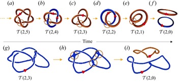


 Open access