


1. Introduction
Jet flows are among the most studied flows in fluid mechanics. Steady jets have a wide array of fundamental studies (List Reference List1982; Gutmark & Grinstein Reference Gutmark and Grinstein1999; Mahesh Reference Mahesh2013), while synthetic jets have been considered only more recently (Glezer & Amitay Reference Glezer and Amitay2002). In application, both steady and unsteady jets are used as flow control devices to prevent flow separation, to enhance mixing, for cooling and heat transfer, and in laminar and turbulence transition (Compton & Johnston Reference Compton and Johnston1992; Mittal & Rampunggoon Reference Mittal and Rampunggoon2002; Pavlova & Amitay Reference Pavlova and Amitay2006; Pavlova, Otani & Amitay Reference Pavlova, Otani and Amitay2008; Kim, Kim & Jung Reference Kim, Kim and Jung2012). Even outside of flow control, steady and unsteady jets exist in nature and engineering as underwater propulsion mechanisms (Van Buren, Floryan & Smits Reference Van Buren, Floryan and Smits2020), in biological flows (Krueger et al. Reference Krueger, Moslemi, Nichols, Bartol and Stewart2009; Jiang, Costello & Colin Reference Jiang, Costello and Colin2021) and even atmospheric or geological flows (Kieffer & Sturtevant Reference Kieffer and Sturtevant1984; Su et al. Reference Su, Hsu, Chen, Wang, Hsiao, Lai, Lee, Sato and Fukunishi2003). Here, our goal is to compare steady and unsteady jets issuing into a laminar boundary layer to better understand their inherent differences in the impact on the surrounding flow.
Steady jets are driven by a constant pressure source, which produces a time-invariant jet of air emitting from the orifice. This jet of air generally begins enclosed by a laminar shear layer, which breaks down subsequently due to instability, and descends into a train of vortex rings and eventually turbulence (List Reference List1982). The circular laminar jet is a classical flow with exact solutions of the Navier–Stokes equations (Schlichting & Gersten Reference Schlichting and Gersten2017). For non-circular cross-sections, the jet flow develops and breaks down rather three-dimensionally, due mostly to the jet asymmetries producing non-uniform advection velocities (Gutmark & Grinstein Reference Gutmark and Grinstein1999).
Unsteady jets have a time-varying velocity at the orifice and can be driven by an oscillating or pulsed (Bidan & Nikitopoulos Reference Bidan and Nikitopoulos2013) pressure source (or sometimes driven by internal instability; Viets Reference Viets1975; Koukpaizan, Glezer & Smith Reference Koukpaizan, Glezer and Smith2021). Note that the term unsteady jet covers a wide array of jet types, including periodic jets and ones with a more arbitrary velocity characteristic. In this work, the unsteady jet is periodic with a zero-mean velocity at the orifice – a specific subset of unsteady jets often referred to as a synthetic jet. Despite there being only one type of unsteady jet, we still use generalized language (i.e. often calling it an unsteady jet instead of a synthetic jet) because, as we will show in this paper, it is the general unsteady nature of the jet that is key in the differences between flow fields produced by oscillating and steady jets.
In synthetic jets, the unsteady forcing produces puffs of high-velocity air and vortex rings that advect away from the orifice (Smith & Glezer Reference Smith and Glezer1998; Van Buren, Whalen & Amitay Reference Van Buren, Whalen and Amitay2014). To form a coherent jet, the frequency and amplitude of the velocity at the orifice need to be within a specific range (Holman et al. Reference Holman, Utturkar, Mittal, Smith and Cattafesta2005). As with the steady jet, the orifice geometry plays a critical role in the unsteady jet formation. For circular orifice synthetic jets, the vortex rings advect normally downstream (Glezer Reference Glezer1988), but when the orifice is rectangular, the vortex ring undergoes axis-switching and breaks down, dependent characteristically on the slot aspect ratio (Dhanak & Bernardinis Reference Dhanak and Bernardinis1981; Van Buren et al. Reference Van Buren, Whalen and Amitay2014).
The direct comparison of steady and synthetic jets in a quiescent fluid has been studied previously (Smith & Swift Reference Smith and Swift2003; Van Buren & Amitay Reference Van Buren and Amitay2016). The main differences are the rate of jet expansion, streamwise momentum generation, and vortical structures. The unsteady nature of the synthetic jet leads to the need to choose a single jet velocity scale, which is especially important when comparing directly to steady jets. The appropriate velocity scaling method depends on the application of the jets (Van Buren & Amitay Reference Van Buren and Amitay2016). Here, the unsteady jet velocity scale,  $U_o$, is calculated using the average jet velocity over the blowing portion of the cycle:
 \begin{equation} U_{o} = \frac{1}{T} \int_0^{T/2} u_j(t)\, \text{d} t = \frac{1}{T} \int_0^{T/2} U_p \sin(2 {\rm \pi}ft)\, \text{d} t = \frac{U_p}{\rm \pi}, \end{equation}
where  $T$ is the time period, $u_j(t)$ is the phase-averaged jet velocity at the orifice exit plane, $U_p$ is the peak jet velocity at the orifice, and $f$ is the actuation frequency of the jet. In a sense, this is saying that the blowing and suction portions of the jet are decoupled, and we are comparing directly the blowing portion of the synthetic jet to the steady jet, effectively ignoring the suction portion. While this is not perfect, we expect that the suction portion plays a much more relaxed role in the resulting flow structure (Van Buren, Smits & Amitay Reference Van Buren, Smits and Amitay2017).
A jet issuing into a crossflow results in complex interactions and vortical structures. A main salient feature of steady jets in a crossflow is a dominant counter-rotating vortex pair that develops downstream (Fric & Roshko Reference Fric and Roshko1994). We will see that for the steady and unsteady jets in this work, the counter-rotating vortex pair remains a major feature of the transverse jet cases. Other secondary flow features of a steady transverse jet include horseshoe vortices due to the boundary layer wrapping around the blockage, re-orienting its vorticity, and the wall-normal wake vortices that extend from the wall to the jet flow itself (Fric & Roshko Reference Fric and Roshko1994). (Most studies have focused on axisymmetric steady jets in a crossflow, and, to our knowledge, no work has explored steady jets in a crossflow from a rectangular orifice of varying orientation.) Unsteady jets issuing into a boundary layer in the past have shown flow features similar to those of steady jets, with the salient feature downstream being dominant streamwise vortices (Bidan & Nikitopoulos Reference Bidan and Nikitopoulos2013). For non-axisymmetric unsteady jets in a boundary layer, the downstream vortex structure is highly dependent on the orifice orientation (Van Buren et al. Reference Van Buren, Leong, Whalen and Amitay2016b). Up to this point, no direct comparison of rectangular steady and unsteady jets in a crossflow has been made, and furthermore, there is no justification in literature for why the two jet types perform differently in preventing flow separation (De Giorgi et al. Reference De Giorgi, De Luca, Ficarella and Marra2015), in reducing drag (Cui et al. Reference Cui, Zhu, Xia and Yang2015), and in heat transfer (Pavlova & Amitay Reference Pavlova and Amitay2006; Farrelly et al. Reference Farrelly, McGuinn, Persoons and Murray2008).
In this work, we compare directly an unsteady and steady jet issuing from a rectangular orifice into a laminar boundary layer. We vary orifice orientation, including multiple pitch (ranging from wall-normal to more aligned with the flow) and skew (ranging from either perpendicular or parallel to the freestream) angles. We will show that the unsteady and steady jets share velocity field features, such as downstream deficit, but the unsteady jet is much more capable of producing vortical structures for matched conditions. Theoretically, we will explore how this difference is rooted in the fundamental difference of the unsteady and steady jet formations. Finally, we will leverage these results for flow control implications like boundary layer momentum addition, enhanced mixing, and jet penetration.
2. Experimental methods
We study experimentally steady and unsteady jets issuing into a laminar flat-plate boundary layer. The flow facility and methods match those of the studies found in Van Buren et al. (Reference Van Buren, Beyar, Leong and Amitay2016a,Reference Van Buren, Leong, Whalen and Amitayb) – we use the same synthetic jet data with the addition of steady jet data for direct comparison. Note that throughout the study, lengths are normalized by the jet orifice width  $h_o = 1$ mm, and velocities are normalized by the wind tunnel freestream velocity $U_\infty =10$ m s $^{-1}$.
The wind tunnel used for this work is an open pull-down tunnel with a  $0.1\ {\rm m} \times 0.1\ {\rm m} \times 0.61\ {\rm m}$ test section. The freestream turbulence is $0.5\,\%$, and the upper wall of the test section is contoured to ensure that there is no streamwise pressure gradient. At the jet location, the boundary layer is laminar with height $\delta _{0.95} = 3$ mm. The jet apparatus was designed to mount into the floor of the wind tunnel; a schematic can be found in figure 1. The steady jet is driven via a constant pressure source, while the synthetic jet is driven via a piezoelectric disk at frequency $f = 1125$ Hz with jet velocity amplitudes $U_p = 5$, 10 and 15 m s $^{-1}$. To generate the synthetic jet, the piezoelectric disk oscillates sinusoidally, which displaces fluid volume periodically, like a piston, inhaling and exhaling fluid through the orifice. The jet orifice is rectangular, $18\ {\rm mm} \times 1\ {\rm mm} \times 6\ {\rm mm}$, with varying pitch angles $\alpha = 45^{\circ }, 65^{\circ }, 90^{\circ }$ and skew angles $\beta = 0^{\circ }, 45^{\circ }, 90^{\circ }$. The jet blowing ratios are in the range $C_b=U_o/U_\infty = 0.5, 1, 1.5$, where the velocity is measured for the wall-normal jet ( $\alpha = 90^{\circ }$) and the volumetric flow is matched, via matching the displaced volume of the piezoelectric disk, to that case for all other orifice pitch angles (this is necessary because the exit area of the jet varies with pitch angle). Subscripts $x$,
$x$,  $y$ and $z$ denote vector components acting along the noted direction. See (1.1) for how the unsteady jet ‘average’ velocity scale is determined.

Figure 1. Jet apparatus used to house both jet types in the wind tunnel floor.
The velocity field was measured using stereoscopic particle image velocimetry to provide two-dimensional planes transverse to the flow with three velocity components. The system was a commercial LaVision system with a dual-head double-pulsed  $120$ mJ Nd:YAG laser and $12$-bit Imager Intenser CCD cameras. The flow was seeded with a Martin Magnum $850$ smoke machine generating particles 1–2 $\mathrm {\mu }$m in diameter. Measurement planes were taken upstream and downstream of the orifice with variable spacing, from $x= -10$ to $20$ every $1$ orifice width, $x = 20$ to $40$ every two orifice widths, and $x=40$ to $90$ every five orifice widths. Data were processed using LaVision software resulting in windows with $209 \times 103$ velocity vectors, with effective resolution (‘probe size’ of measurement) $0.61~{\rm mm} \times 0.7~{\rm mm}$ in the $y$ and $z$ directions, respectively. For time-averaged results, $500$ image pairs are averaged, and for phase-averaged results (unsteady jet only), the data acquisition was phase-locked to the jet at phases $\phi = 0^{\circ }$– $315^{\circ }$ every $45^{\circ }$, and $250$ image pairs are averaged. Guidelines provided by Adrian & Westerweel (Reference Adrian and Westerweel2011) were followed throughout the experiment to minimize measurement uncertainty. Assuming a spatial error of $0.1$ pixels (Adrian & Westerweel Reference Adrian and Westerweel2011), the errors in the velocity measurements for the present experiment were $\pm 0.2$– $0.6$ m s $^{-1}$, corresponding to time delays $\Delta t = 1$– $10\ \mathrm {\mu }$s. Supplementary materials are available at https://doi.org/10.1017/jfm.2022.413; for the experimental set-up, see Van Buren et al. (Reference Van Buren, Leong, Whalen and Amitay2016b).
3. Results and discussion
3.1. Flow field characterization
Our analysis begins with qualitative comparisons between the two jets, focused on the changes in streamwise velocity, streamwise vorticity and coherent vortical structures. There are a total of nine combinations of pitch and skew angles for the steady and unsteady jets; detailing and discussing the flow field of each would not be within the scope of this paper. Here we explore three representative orifice orientations in detail for both jets: where the orifice is: (1) wall-normal to the wind tunnel floor,  $\alpha = 90^{\circ }$, and perpendicular to the crossflow, $\beta = 0^{\circ }$ (see figure 2); (2) wall-normal to the wind tunnel floor, $\alpha = 90^{\circ }$, and parallel to the crossflow, $\beta = 90^{\circ }$ (see figure 3); (3) angled relative to the floor, $\alpha = 45^{\circ }$, and perpendicular to the crossflow, $\beta = 0^{\circ }$ (see figure 4). They represent the most popular orifice orientation cases, most important for flow control implications that we will see later on, and also the most extreme in terms of their impact on the flow. For the complete collection of flow field contours, see the supplementary material accompanying this paper.

Figure 2. (a) Change in velocity, (b) streamwise vorticity, and (c) vortical structures for the steady (top) and unsteady (bottom) jets for  $C_b=1.5$ at $\alpha =90^{\circ }$ and $\beta =0^{\circ }$. The steady and unsteady jets share the same scale except in (c).

Figure 3. (a) Change in velocity, (b) streamwise vorticity, and (c) vortical structures for the steady (top) and unsteady (bottom) jets for  $C_b=1.5$ at $\alpha =90^{\circ }$ and $\beta =90^{\circ }$. The steady and unsteady jets share the same scale except in (c).

Figure 4. (a) Change in velocity, (b) streamwise vorticity, and (c) vortical structures for the steady (top) and unsteady (bottom) jets for  $C_b=1.5$ at $\alpha =45^{\circ }$ and $\beta =0^{\circ }$. The steady and unsteady jets share the same scale except in (c).
Downstream development of the change in velocity field induced by the steady and unsteady jet is shown in figures 2(a), 3(a) and 4(a). The baseline flow (i.e. no jet activated) was subtracted from the flow field when the jet was active. In the wall-normal cases,  $\alpha =90^{\circ }$, both steady and unsteady jets create distinct regions of blockage extending far downstream. Generally, this is a salient feature of wall-normal jets issuing into a flow field; the incoming flow is redirected around the jet, and the jet produces a wake region with velocity deficit. For the wall-normal case where the orifice is parallel to the freestream, $\beta =90^{\circ }$ (figure 3), the impact of the jet extends further from the wall and seems to detach from the wall entirely downstream. Notably, for the unsteady jet, there are also regions of accelerated flow neighbouring the deficit near the freestream. In the case where the jet is directed downstream, $\alpha =45^{\circ }$ (figure 4), there are only large regions of direct increased velocity. This is because the jet itself adds to the freestream. Finally, we notice that both jets increase the velocity near the wall, especially for $\alpha =90^{\circ }$, $\beta =0^{\circ }$ (figure 2), and these regions of near-wall acceleration grow downstream as the wake diminishes. Generally, the change in velocity field is quite similar between the steady and unsteady jets; however, the regions of accelerated flow are more forceful for the unsteady jet.
When considering the vorticity field, shown in figures 2(b), 3(b) and 4(b), the steady and unsteady jets are vastly different in strength. Note that for clarity, regions of very low vorticity ( $-0.05 \leq \omega _x \leq 0.05$) were suppressed. Both the steady and unsteady jets produce paired regions of positive and negative streamwise vorticity, symmetric about the orifice centreline. (For other orifice orientations, the vorticity is still similar but not necessarily symmetric about the centreline, as in Van Buren et al. Reference Van Buren, Leong, Whalen and Amitay2016b.) Steady jets produce weaker vorticity concentrations, whereas unsteady jets exhibit much stronger vorticity that persists further downstream and extends further into the freestream. The unsteady jet vorticity coalesces to form quasi-steady streamwise rollers downstream of the orifice (Van Buren et al. Reference Van Buren, Beyar, Leong and Amitay2016a). Here, the strongest vorticity concentrations come from the case where the jet is wall-normal, $\alpha =90^{\circ }$, and parallel to the flow, $\beta =90^{\circ }$, because more of the orifice, which emits the jet vorticity directly, is aligned with the streamwise direction. The weakest vorticity concentrations come from the case where the jet is tilted into the flow, $\alpha =45^{\circ }$, because the orifice contains the least amount of streamwise-oriented vorticity. In general, the vorticity field exhibits a stark contrast between the two jet types – similar structures but different strengths.
One of the main features of jets in a crossflow is the coherent streamwise vortical structures produced. We compare the vortex structure of the steady jets to the unsteady jet using the  $\mathcal {Q}$-criterion (Hunt, Wray & Moin Reference Hunt, Wray and Moin1988), which represents the vorticity with strain-dominant or rotation-dominant components. While the $\mathcal {Q}$-criterion is typically a scalar, we calculate the rotation from only the streamwise vorticity and give it the sign of the local vorticity, which is deemed $q_x$. Figures 2(c), 3(c) and 4(c) show the streamwise vortex structure downstream development for the steady and unsteady jets. Note here that the strengths of the structures were so different that we needed independent colour scales for each, where the steady jet colour scale is 10 times lower than that of the unsteady jet. As before with the vorticity, low-strength regions were suppressed for the unsteady ( $-0.05 \leq q_x \leq 0.05$) and steady ( $-0.005 \leq q_x \leq 0.005$) jets. Clearly, the unsteady jet produces a much stronger and more coherent streamwise vortex structure when compared to the steady jets, for all geometries considered. The unsteady jet vortex pair extends throughout the plotted domain, and strong vortices are present even 30 orifice widths downstream. The unsteady jets also exhibit secondary streamwise vortical structures above the main vortical structures (up to $x = 15$) for $\alpha = 90^{\circ }$, $\beta = 0^{\circ }$ (figure 2c), that are not present for the steady jet. These secondary structures are unsteady and decay more rapidly than the streamwise rollers exhibited by both jets (Van Buren et al. Reference Van Buren, Beyar, Leong and Amitay2016a). Asymmetric vortical structures about $z = 0$ (figures 5 $i.c$, $ii.c$) are caused by the jet pitch angle. The jets are emitting to the side and creating vortical structures that are vectored away from the orifice centre. Generally, it appears that the higher peak vorticity paired with the cyclic nature of unsteady jets facilitates much stronger rotational structures. This is due to the fundamental differences in jet formation: steady jets produce shear layers that break down into vortex structure, whereas unsteady jets, like this synthetic jet, produce a train of vortex rings that coalesce into a jet.

Figure 5. Contours of streamwise  $\mathcal {Q}$, $q_x$, at $x = 6$ for $C_b = 1.5$ and each jet orientation: pitch angles $\alpha = 45^{\circ }, 65^{\circ }, 90^{\circ }$ ( $i$–
$i$– $iii$), and skew angles $\beta = 0^{\circ }, 45^{\circ }, 90^{\circ }$ ( $a$–
$a$– $c$). The upper portions of the graphs correspond to steady jets, while the lower halves show the unsteady jets. Solid and dashed lines correspond to positive (counter-clockwise) and negative (clockwise) rotation, respectively.
To confirm that the vortex strength difference between steady and unsteady jets is consistent for all orifice orientations, the vortex structure is plotted in figure 5 at  $x=6$ downstream of the orifice for the nine pitch angle and skew angle combinations. The steady and unsteady jets are compared on the top and bottom of each plot, respectively. To make qualitative comparisons, the unsteady jet vortex contours are much stronger than the steady jet contours, and each is scaled independently – the steady jet contours are $50$ times weaker than the unsteady jet contours. First, the unsteady jet vortical structures are generally more cohesive, exhibiting larger and clearer structures. However, the unsteady and steady jet vortex structures are largely similar in shape and organization. It is clear that over the entire range of orifice orientations studied here, steady and unsteady jets produce similar structures, but the unsteady jet produces much stronger versions of those structures.
The choice of velocity scaling is critical when comparing unsteady and steady jets, and often different scalings are appropriate in different applications. Thus far, we have considered only a single scaling of the oscillating jet velocity: the average of the blowing cycle as described in (1.1). However, an argument can be made for other velocity scaling parameters based on the peak jet velocity (Kral et al. Reference Kral, Donovan, Cain and Cary1997) or the jet momentum (Cater & Soria Reference Cater and Soria2002). For example, the jet momentum velocity scaling can be appropriate when used to match jet circulation. For quiescent flows, the scaling of a synthetic jet and a steady jet are compared in Van Buren & Amitay (Reference Van Buren and Amitay2016). In Appendix A, we have explored several different scaling parameters for a crossflow when comparing the steady and unsteady jets on parameters such as wake, circulation and vortex structure. Interestingly, the momentum velocity scaling is best at making the circulation more comparable between the steady and unsteady jets. However, no known traditional velocity scaling method caused the steady jets to have more comparable vortex structure, thus there are inherent differences between the two jet types that are not captured by scaling choice.
3.2. Theory and statistics
We seek a theoretical explanation for the difference in steady and unsteady jet impacts – specifically, why the unsteady jet produces more prominent vortical structures. Here, we use a simplified laminar flat-plate boundary layer flow model to estimate roughly the flow on the inner walls of the jet orifice (Schlichting & Gersten Reference Schlichting and Gersten2017). In reality, the flow through the orifice can be complex, with separation along the orifice walls as well as inlet and exit effects. While there are major differences between simple theory and reality, we still find boundary layer models useful in illuminating the key reason for the stark differences between the peak vorticities produced by the unsteady and steady jets.
The differences in vorticity generation result from differences in the discharge characteristics: synthetic jets produce trains of vortex rings, while steady jets produce steady vortex sheets.
Consider the jet formation in the flow through the orifice. The vorticity produced by the jets and added to the freestream is generated primarily on the inner orifice walls housing the flow between the jet cavity and the external flow. In essence, the competition of unsteady and steady jets is a competition of Stokes and Blasius boundary layers on the orifice walls. The Stokes problem is that of a fully developed laminar flow due to an oscillating freestream above a flat plate, and Blasius studied a developing laminar flow due to a steady freestream over a flat plate – both of which have known solutions (Schlichting & Gersten Reference Schlichting and Gersten2017). Loosely, these are representative of the scenario for unsteady and steady jets. Theoretical solutions have also been found for arbitrary wall velocities, showing that generally, unsteady flows lead to higher velocity gradients and peak vorticity (Schlichting & Gersten Reference Schlichting and Gersten2017). We can compare directly, analytically, the peak vorticities at the wall due to these two flows. It is important to note that we focus on the peak vorticity, or vorticity at the wall, as the main metric in comparing unsteady and steady jets here. We believe that it is the higher peak vorticity in more concentrated areas that leads to the more prolific vortical structures downstream. The vorticity at the wall for a Blasius boundary layer is
 \begin{equation} \omega_{x_{B}} = 0.332 \sqrt{\frac{U_o^{3}}{\nu x}}, \end{equation}
and the peak wall vorticity for a Stokes boundary layer is
 \begin{equation} \omega_{x_{S}} = \sqrt{ \frac{2 {\rm \pi}f}{\nu}}\,U_o. \end{equation}
The ratio of the two wall vorticities results in a non-dimensional parameter that describes whether the steady or unsteady case has the dominant vorticity based upon input parameters:
 \begin{equation} \frac{\omega_{x_{S}}}{\omega_{x_{B}}} = 7.55 \sqrt{\frac{x f}{U_o}}. \end{equation}
This is essentially a non-dimensional frequency, where the time scale of the oscillation is compared to the time scale of the flight of a particle along the wall. Here, when the frequency is high for the Stokes flow, or when the development length for the Blasius flow is large, the oscillating boundary layer wall vorticity will dominate.
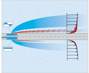
We compare the theoretical wall vorticity along our orifice wall for the steady and unsteady cases in figure 6. For the frequency, jet velocity and geometry in this work, this comparison indicates we should see peak streamwise vorticity values that are approximately five times higher than the steady jet at the end of the orifice. This is borne out by our results in figure 2, where the peak vorticity for the unsteady jet case is about two times greater than in the steady case. This root difference in flow through the orifice is the main contributor to differences in downstream vorticity and vortex structure that were measured. The unsteady nature of the jet increases the generated vorticity intrinsically.

Figure 6. Vorticity ratio between the Stokes and Blasius boundary layer solutions. Inset is the boundary layer profile at the end of the orifice neck for both flow regimes.
An interesting consequence of this is that among unsteady jets, the peak vorticity and subsequent downstream steady vortex structure will be dependent on the jet frequency. It seems that frequency (not associated with characteristic flow instabilities) might play a role in flow control effectiveness.
3.2.1. Vorticity transport
Once vorticity is generated at the orifice walls, it is expelled by the jet into the flow. From here, the vorticity transport can be used to show what specific flow features contribute to the vorticity development downstream. First, consider the incompressible form of the streamwise vorticity transport equation (Tennekes & Lumley Reference Tennekes and Lumley1972):
 \begin{align} &\frac{\partial \omega_x}{\partial t} + u_x\,\frac{\partial \omega_x}{\partial x} + u_y\, \frac{\partial \omega_x}{\partial y} + u_z\,\frac{\partial \omega_x}{\partial z} = \omega_x\, \frac{\partial u_x}{\partial x} + \omega_y\,\frac{\partial u_x}{\partial y} + \omega_z\, \frac{\partial u_x}{\partial z} \nonumber\\ &\quad + \nu \left( \frac{\partial^{2} \omega_x}{\partial x^{2}} + \frac{\partial^{2} \omega_x}{\partial y^{2}} + \frac{\partial^{2} \omega_x}{\partial z^{2}}\right). \end{align}
Our data set is limited in spatial resolution, with good resolution in the  $y$ and $z$ directions, but poor resolution in the streamwise $x$ direction (due to the spacing of the acquisition planes and the laser sheet thickness, $\approx 1$ mm). As a result, we can adequately resolve only the streamwise vorticity $\omega _x$ and the three velocity components. Additionally, while our resolution in the data plane $y$–
$y$– $z$ is good, it is not sufficient for second-order spatial derivatives. So we are limited to exploring only the left-hand side of the vorticity transport equation (3.4), which is the material derivative of the streamwise vorticity ${\rm D} \omega _x/{\rm D}t$. We move forward with our analysis with the reservation that we can describe only the vorticity development and not the vortex tilting/stretching and viscous diffusion terms.
The unsteady jet has a known coherent frequency component, so we will employ the triple decomposition of velocity into the mean  $\bar {u}$, coherent $\tilde {u}$, and unsteady $u'$ components:
 \begin{equation} u = \bar{u} + \tilde{u} + u'. \end{equation}
Note that this decomposes the vorticity similarly. Our data were acquired and either time-averaged (denoted with overlined terms, e.g.  $\bar {x}$) or phase-averaged (denoted with angle-bracket terms, e.g. $\langle x \rangle$). If we apply the triple decomposition (3.5) to the material derivative in the vorticity transport equation (3.4), and then time-average, then we get
 \begin{align} \overline{\frac{{\rm D} \omega_x}{{\rm D} t}} &= \overline{\frac{\partial \bar{u}_x\bar{\omega}_x}{\partial x}} + \overline{\frac{\partial \tilde{u}_x\tilde{\omega}_x}{\partial x}} + \overline{\frac{\partial {u_x'}{\omega_x'}}{\partial x}} + \overline{\frac{\partial \bar{u}_y\bar{\omega}_x}{\partial y}} + \overline{\frac{\partial \tilde{u}_y\tilde{\omega}_x}{\partial y}} + \overline{\frac{\partial {u_y'}{\omega_x'}}{\partial y}} \nonumber\\ &\quad + \overline{\frac{\partial \bar{u}_z\bar{\omega}_x}{\partial z}} + \overline{\frac{\partial \tilde{u}_z\tilde{\omega}_x}{\partial z}} + \overline{\frac{\partial {u_z'}{\omega_x'}}{\partial z}}. \end{align}
Alternatively, if we phase-average, then we get
 \begin{align} &\left\langle\frac{{\rm D} \omega_x}{{\rm D} t}\right\rangle = \left\langle \frac{\partial \tilde{\omega}_x}{\partial t}\right\rangle + \left\langle \frac{\partial \bar{u}_x \bar{\omega}_x}{\partial x} + \frac{\partial \bar{u}_x \tilde{\omega}_x}{\partial x} + \frac{\partial \tilde{u}_x \bar{\omega}_x}{\partial x} + \frac{\partial \tilde{u}_x \tilde{\omega}_x}{\partial x}\right\rangle \nonumber\\ &\quad +\left\langle \frac{\partial \bar{u}_y \bar{\omega}_x}{\partial y} + \frac{\partial \bar{u}_y \tilde{\omega}_x}{\partial y} + \frac{\partial \tilde{u}_y \bar{\omega}_x}{\partial y} + \frac{\partial \tilde{u}_y \tilde{\omega}_x}{\partial y}\right\rangle + \left\langle \frac{\partial \bar{u}_z \bar{\omega}_x}{\partial z} + \frac{\partial \bar{u}_z \tilde{\omega}_x}{\partial z} + \frac{\partial \tilde{u}_z \bar{\omega}_x}{\partial z} + \frac{\partial \tilde{u}_z \tilde{\omega}_x}{\partial z}\right\rangle. \end{align}
The complete procedure for the averaging schemes can be found in Appendices B and C. While we present the terms with the products of two unsteady fluctuations (e.g.  $u_x'\omega _x'$), we do not have the sample size to explore statistically converged turbulence, so we ignore these terms, though we anticipate that they will be insignificant because the flow is laminar. These two equations – the time-averaged (3.6) and phase-averaged (3.7) simplified vorticity transport equations with triple decomposition – describe our current data set.
Figure 7 presents a comparison of the downstream development of all the terms of the time-averaged vorticity transport equation (3.6). The terms were area-averaged at each streamwise location. All terms generally peak near the orifice and tend to decay downstream. Comparing the terms between steady and unsteady jets, the unsteady jet has greater vorticity transport in all geometries. Interestingly, there are no standout dominant terms; both the products of the means and the products of the coherent fluctuations are contributing meaningfully to the downstream vorticity transport through all geometries.

Figure 7. Downstream development of the vorticity terms for  $C_b = 1.5$. Here, (a–c) represent a fixed skew angle ( $\beta = 0^{\circ }$) and increasing pitch angle ( $\alpha = 45^{\circ }, 65^{\circ }, 90^{\circ }$). Additionally, (d) and (e) correspond to a fixed wall-normal pitch angle ( $\alpha = 90^{\circ }$) with skew angles $\beta = 45^{\circ },90^{\circ }$, respectively. Inset are pie charts showing the term contributions over the entire streamwise domain.
In figure 8, the terms of the phase-averaged vorticity transport equation (3.7) are compared. Note that these terms apply to only the unsteady jet as the steady jet does not have any phase-locked variance. As with the time-averaged terms, the phase-averaged terms are area-averaged at each streamwise location. Here, the time-derivative vorticity term is clearly dominant throughout the downstream development across all geometries. This indicates that the time-varying vorticity term is a major contributor to vorticity transport with the unsteady jet and is the culprit for the enhanced flow vorticity when compared to the steady jet. This ties back to the Stokes and Blasius comparison that predicted that time-varying velocities lead to much higher peak vorticity that is inherently time-varying.

Figure 8. Phase-averaged vorticity equation streamwise development for  $C_b = 1.5$. Here, (a–c) represent a fixed skew angle ( $\beta = 0^{\circ }$) and increasing pitch angle ( $\alpha = 45^{\circ }, 65^{\circ }, 90^{\circ }$). Additionally, (d) and (e) correspond to a fixed wall-normal pitch angle ( $\alpha = 90^{\circ }$) with skew angles $\beta = 45^{\circ },90^{\circ }$, respectively. Inset are pie charts showing the term contributions over the entire streamwise domain.
In the phase-averaged vorticity transport, the pitch angle has a large impact on the overall vorticity generated. When the unsteady jet is angled into the flow, the time rate of change of vorticity is lowest – less than half of the wall-normal case. This is because as the jet is angled, the orifice vorticity gains a larger component in the wall-normal direction, so there is less injection of streamwise vorticity. The added vorticity is less sensitive to skew angle.
3.3. Flow control implications
Finally, we consider the implications of these results to flow control application. We look at three parameters: (1) added momentum into the boundary layer, which is a measure of flow separation resilience; (2) added vorticity strength, which indicates enhanced mixing and turbulence; and (3) wall penetration, which is a metric that has been considered more recently for targeted structure control. All three parameters guide implementation methods as flow control devices.
The added momentum near the wall within the boundary layer is tied directly to the flow's ability to resist separation (Smith Reference Smith2002). The baseline normalized near-wall momentum,  $\bar {P}_{\delta _{0.95}}$, was calculated according to
 \begin{equation} \bar{P}_{\delta_{0.95}} = \frac{1}{(2 l_o) h_o} \int_{{z}_{{min}}}^{{z}_{{max}}}\int_0^{\delta_{0.95}} \frac{U_x^{2}}{U_{x_b}^{2}} \, {{\rm d} y}\, {{\rm d}z}, \end{equation}
where the subscript  $b$ refers to the baseline case. Note that in the equation, we have added the bounds in the $y$ integration to be within the near-wall region, defined by the baseline boundary layer, whereas for the $z$ direction we consider the entire data window. Figure 9( $I$) shows the downstream development of the added momentum in the boundary layer for the steady and unsteady jets. Downstream of the orifice, the boundary layer momentum was heavily influenced by the orifice orientation. Both the steady and unsteady jets created local increases and decreases in momentum. Downstream, away from the orifice, the unsteady jet generally adds momentum into the boundary layer, while the steady jet has little impact. For most cases, the unsteady jet produces greater boundary layer acceleration than the steady jet. This is likely due to the enhanced vortex structure of the unsteady jet pulling high momentum fluid into the boundary layer, much as a vortex generator would. (Interestingly, synthetic jets are better vortex generators than actual passive vortex generators; Van Buren, Whalen & Amitay Reference Van Buren, Whalen and Amitay2015.) However, this is not the only mechanism for adding boundary layer momentum. For orifice pitch angles where the jet is more aligned with the flow, the jet can add streamwise momentum directly. These are the cases where we see a net acceleration in the boundary layer for the steady jet. However, there are outlier cases where the steady jet exceeds the unsteady jet, specifically the streamwise-aligned orifice orientations ( $\beta = 90^{\circ }$). This is because in these cases, the steady jets produce their strongest vortical structure, more comparable to the unsteady jet vortex structure. Added boundary layer momentum is dependent on jet trajectory and vortical structure generation, among other things, thus it is difficult to find clear behaviours with parametric changes in orifice orientation. Even in more detailed investigations of unsteady jets with similar geometries, there is a lack of clear trends with orifice orientation (Van Buren et al. Reference Van Buren, Leong, Whalen and Amitay2016b).

Figure 9. Flow statistics development downstream of the orifice:  $(I)$ normalized near-wall added momentum, $(II)$ enstrophy, and $(III)$ boundary layer normalized jet penetration for $C_b = 1.5$. Each row represents a single jet orientation: pitch angles $\alpha = 45^{\circ }, 65^{\circ }, 90^{\circ }$ ( $i$–
$i$– $iii$) and skew angles $\beta = 0^{\circ }, 45^{\circ }, 90^{\circ }$ ( $a$–
$a$– $c$).
$c$).
Next, we consider the jet mixing, which can not only delay separation (Rediniotis et al. Reference Rediniotis, Ko, Yue and Kurdila1999), but also enhance heat transfer (Farrelly et al. Reference Farrelly, McGuinn, Persoons and Murray2008) and enhance turbulence (Compton & Johnston Reference Compton and Johnston1992). Here we represent mixing through the flow streamwise enstrophy
 \begin{equation} \varepsilon_x = \frac{1}{2}\iint\omega_x^{2} \,{{\rm d} y} \,{{\rm d}z},\end{equation}
which is essentially the strength in vorticity and is calculated over the entire domain. The downstream development of the enstrophy is shown in figure 9( $II$). For both jets, enstrophy peaks near the orifice and decays downstream. This behaviour follows the same trend shown in the vorticity flow visualization in figure 2(b). It is quite clear that – throughout the entire parameter space and measurement domain – the unsteady jet dominates the added vorticity to the flow. This is no surprise; to this point, the theme of the results has been the unsteady jet's capability to produce strong, coherent vortical structures compared to the steady jet. This is due to the fundamental differences in how the unsteady jet is generated (see § 3.2).
Finally, a parameter often explored in jets is the wall-normal penetration, which has implications for specific types of flow control that target structures away from the wall, e.g. large-scale motion control in turbulent boundary layers. The scaling of synthetic jet penetration has been studied extensively (Berk et al. Reference Berk, Hutchins, Marusic and Ganapathisubramani2018; Jankee & Ganapathisubramani Reference Jankee and Ganapathisubramani2021). Jet unsteadiness affects the jet trajectory, and when the distance between pulses  $U_\infty /f$ nears the jet slot size, steady jet scaling arguments can be applied to unsteady jets (Berk et al. Reference Berk, Hutchins, Marusic and Ganapathisubramani2018). While there are multiple methods for determining jet trajectory, for simple comparison we use the wall-normal centroid of the change in spanwise-averaged streamwise velocity (spanwise-averaging denoted by $\langle \Delta U_x \rangle _z$):
 \begin{equation} y_c = \frac{\displaystyle \sum_{y=0}^{y=y_{{max}}} y \left\langle \Delta U_x \right\rangle_z}{\displaystyle \sum_{y=0}^{y=y_{{max}}} \left\langle \Delta U_x \right\rangle_z}. \end{equation}
For this specific parameter, the jet location was non-dimensionalized by the baseline boundary layer height  $\delta _{0.95}$ so that it is easy to assess how well the jets are able to penetrate the boundary layer. The wall-normal penetration of the jets is shown in figure 9( $III$). In one case, figure 9( $III(iii,c)$), the unsteady jet wake leaves the measurement domain, skewing the resulting trajectory calculation. This region begins around $x = 20$ and is represented with a dashed line. Generally, the steady and unsteady jets are able to penetrate above the boundary layer at this blowing ratio. The differences between the steady and unsteady jets here are subtle. For most cases, the unsteady jet slightly exceeds the steady jet. However, the steady jets with an orifice skew angle more aligned with the flow penetrate further into the freestream than the unsteady jets. Ultimately, the penetration is largely similar for both steady and unsteady jets, which is tied directly to the similar velocity fields produced – as was characterized in § 3.1.
4. Summary and conclusions
Steady and unsteady rectangular jets were issued into a laminar boundary layer and explored experimentally using stereoscopic particle image velocimetry. The jet orifice orientation was varied in pitch (from wall-normal to more aligned with the flow) and skew (from across to along the flow). Multiple jet strengths were tested, though they produced no difference in trends, only differences in the strength of the jet impact. All data are made available through supplementary material associated with this work.
Qualitatively, both jets produced similar effects on the velocity field, including the strength and size of the deficit region downstream of the orifice. Despite this, unsteady jets formed stronger vorticity than the steady jet counterpart. As a result, the unsteady jet produced much stronger and more cohesive vortex structures than the steady jet, though they both produced similar qualitative vortex organization. This behaviour was consistent for all orifice orientations and blowing ratios in this study. Note that we tested multiple velocity scaling methods to ensure that these differences were not merely rooted in the definition of average unsteady jet velocity.
The reason why unsteady jets produced considerably more coherent vortex structure than steady jets was rooted in the fundamental vorticity generation mechanism. As flow passes through the jet orifice, the no-slip condition produces a boundary layer – either a Blasius boundary layer for the steady jet, or a Stokes layer for the unsteady jet. A simple theoretical analysis showed that the Stokes layer intrinsically produces higher vorticity than the Blasius layer, and thus the unsteady jet ejects more vorticity into the crossflow than the steady jet for matched velocity conditions. These results were then further confirmed via analysis of the vorticity transport equations in either their time-averaged or phase-averaged form. This stronger vorticity couples with the fact that steady jets produce shear layers that break down into vortex structure, whereas unsteady jets, like the synthetic jet, start with vortex structures that form a jet downstream (Van Buren & Amitay Reference Van Buren and Amitay2016).
To summarize the flow control implications, unsteady jets added more momentum to the boundary layer than steady jets, likely due to the enhanced coherent vortex structure. This indicates that unsteady jets will be more capable at mitigating separation, especially in a transverse configuration. The best cases for added momentum were low pitch angles ( $\alpha =45^{\circ }$) where the jet momentum is more directly aligned with the streamwise direction. Unsteady jets, by far, produced more enstrophy from streamwise vorticity, indicating that unsteady jets will be more capable of inducing flow mixing. The best orifice orientation for added streamwise vorticity was when the orifice was along the flow ( $\beta =90^{\circ }$), due to the long edge of the orifice, which contains more orifice boundary layer vorticity, being in the streamwise direction. Finally, steady and unsteady jets produced similar penetration characteristics, indicating that the penetration is tied to the velocity field. Higher jet penetrations occurred when the orifice was along the flow ( $\beta =90^{\circ }$) because the cross-sectional area of the jet was smallest and least impacted by the crossflow.
While in application the jet choice is certainly up to the user, there are clear foundational differences between steady and unsteady jets when issued into a crossflow that should be considered.
Supplementary material
Supplementary material is available at https://doi.org/10.1017/jfm.2022.413.
Declaration of interests
The authors report no conflict of interest.
Appendix A. Velocity scaling methods
We have been discussing a velocity scaling method where the unsteady jet output was defined as the average velocity over the blowing cycle, (1.1). However, an argument can be made for at least two additional scaling metrics: (1) the peak velocity of the jet,  $U_p$; and (2) the average momentum velocity over the whole cycle.
To compare each method, we look at the velocity difference, streamwise vorticity and vortex structure. To compare each flow statistic more easily, the area averages of the absolute values were used; see figure 10. The velocity difference stands out as the most impacted feature when compared to previous discussions. The steady jet has a much greater impact on the velocity field for both alternative scaling methods. We can compare directly our original scaling method here by looking at the first case for the steady jet and the final case for the unsteady jet. The similar velocity difference between these two cases was originally shown through the flow field visualization in § 3.1.

Figure 10. Average values of (a) velocity difference, (b) streamwise vorticity, and (c) vortex structure, over the entire domain. The labelled output velocities refer to matched (1) peak jet velocity,  $U_p$, and (2) average momentum velocity over the whole cycle, $2U_p/{\rm \pi}$.
When matching peak jet velocity, the steady jet produced more vorticity than the unsteady jet. Here, we quantify the vorticity production in a similar manner to how circulation is calculated, as an area average, except that we use the absolute value of vorticity. However, for the momentum scaling, the unsteady jet was either about equal or better at generating vorticity. For all velocity scaling methods, the rotational structures are stronger for the unsteady jets. This is despite the stronger vorticity from steady jets when matching peak velocity. Higher vorticity does not necessarily translate to stronger and more coherent vortex structures.
Appendix B. Reynolds-averaged vorticity equation
Here, we apply Reynolds-averaging (Reynolds Reference Reynolds1895) to the vorticity equation to derive the equation used in § 3.2.1. While a simplified version was presented, this derivation is done using tensor notation, where  $i$ is the free index and $j$ is the dummy variable. Due to the coherent fluctuations for the unsteady jets, triple decomposition of the velocity field is used instead of double decomposition. First, we begin with the vorticity equation for an incompressible fluid (Tennekes & Lumley Reference Tennekes and Lumley1972):
 \begin{equation} \frac{{\rm D} \omega_i}{{\rm D} t} = \frac{\partial \omega_i}{\partial t} + u_j\,\frac{\partial \omega_i}{\partial x_j} = (\omega_j \boldsymbol{\cdot} \boldsymbol{\nabla} ) u_i + \nu\,\nabla^{2} \omega_i. \end{equation}
In addition to this equation, the continuity equation for an incompressible fluid is also used:
 \begin{equation} \frac{\partial u_x}{\partial x} + \frac{\partial u_y}{\partial y} + \frac{\partial u_z}{\partial z} = 0. \end{equation}
Using the product rule, the continuity equation can be isolated, and we also see that the first three terms on the right-hand side look like terms that appear in the vorticity equation:
 \begin{align} \frac{\partial u_x \omega_x}{\partial x} + \frac{\partial u_y \omega_y}{\partial y} + \frac{\partial u_z \omega_z}{\partial z} = u_x\,\frac{\partial \omega_x}{\partial x} + u_y\, \frac{\partial \omega_y}{\partial y} + u_z\,\frac{\partial \omega_z}{\partial z} + \omega_x \left[ \frac{\partial u_x}{\partial x} + \frac{\partial u_y}{\partial y} + \frac{\partial u_z}{\partial z} \right]. \end{align}
Terms inside the square brackets are the same terms that appear in the continuity equation, therefore, that bracketed section is equal to zero. This procedure allows for terms to be combined inside the partial derivative:
 \begin{equation} \frac{\partial u_x \omega_x}{\partial x} + \frac{\partial u_y \omega_y}{\partial y} + \frac{\partial u_z \omega_z}{\partial z} = u_x\,\frac{\partial \omega_x}{\partial x} + u_y\, \frac{\partial \omega_y}{\partial y} + u_z\,\frac{\partial \omega_z}{\partial z}. \end{equation}
We can leverage this to obtain a new form of the vorticity equation:
 \begin{equation} \frac{\partial \omega_i}{\partial t} + u_j\,\frac{\partial \omega_i}{\partial x_j} = \frac{\partial \omega_i}{\partial t} + \frac{\partial u_j \omega_i}{\partial x_j}. \end{equation}
This form is used for both the time- and phase-averaging. Due to the large number of terms, applying the triple decomposition and time-averaging is done to one side of the equation at a time. We start with the material derivative:
 \begin{align} &\overline{ \frac{\partial \bar{\omega}_i}{\partial t} + \frac{\partial \tilde{\omega}_i}{\partial t} + \frac{\partial \omega_i'}{\partial t} + \frac{\partial \bar{u}_j \bar{\omega}_i}{\partial x_j} + \frac{\partial \bar{u}_j \tilde{\omega}_i}{\partial x_j} + \frac{\partial \bar{u}_j {\omega}_i'}{\partial x_j}} \nonumber\\ &\quad +\overline{\frac{\partial \tilde{u}_j \bar{\omega}_i}{\partial x_j} + \frac{\partial \tilde{u}_j \tilde{\omega}_i}{\partial x_j} + \frac{\partial \tilde{u}_j {\omega}_i'}{\partial x_j} + \frac{\partial {u}_j' \bar{\omega}_i}{\partial x_j} + \frac{\partial {u}_j' \tilde{\omega}_i}{\partial x_j} + \frac{\partial {u}_j' {\omega}_i'}{\partial x_j} }. \end{align}
Time averages of fluctuation terms and uncorrelated fluctuation products are equal to zero (Reynolds Reference Reynolds1895). The following non-zero terms remained:
 \begin{equation} \overline{\frac{\partial \bar{u}_j \bar{\omega}_i}{\partial x_j} + \frac{\partial \tilde{u}_j \tilde{\omega}_i}{\partial x_j} + \frac{\partial {u}_j' {\omega}_i'}{\partial x_j}}. \end{equation}
The above procedure was then repeated for the right-hand side of the vorticity equation:
 \begin{align} &\overline{ \bar{\omega}_j\,\frac{\partial \bar{u}_i}{\partial x_j} + \tilde{\omega}_j\,\frac{\partial \bar{u}_i}{\partial x_j} + {\omega}_j'\,\frac{\partial \bar{u}_i}{\partial x_j} + \bar{\omega}_j\, \frac{\partial \tilde{u}_i}{\partial x_j} + \tilde{\omega}_j\,\frac{\partial \tilde{u}_i}{\partial x_j} + {\omega}_j'\,\frac{\partial \tilde{u}_i}{\partial x_j} + \bar{\omega}_j\,\frac{\partial u_i'}{\partial x_j} + \tilde{\omega}_j\,\frac{\partial u_i'}{\partial x_j} + {\omega}_j'\, \frac{\partial u_i'}{\partial x_j}} \nonumber\\ &\quad \overline{+ \nu \left[ \frac{\partial^{2} \bar{\omega}_i}{\partial x_j^{2}} + \frac{\partial^{2} \tilde{\omega}_i}{\partial x_j^{2}} + \frac{\partial^{2} {\omega}_i'}{\partial x_j^{2}} \right] }. \end{align}
Enforcing the same rules as before, this now reduces to four terms:
 \begin{equation} \overline{ \bar{\omega}_j\,\frac{\partial \overline{u_i}}{\partial x_j} + \tilde{\omega}_j\, \frac{\partial \widetilde{u_i}}{\partial x_j} + {\omega}_j'\,\frac{\partial {u_i}'}{\partial x_j} + \nu\,\frac{\partial^{2} \bar{\omega}_i}{\partial x_j^{2}} }. \end{equation}
The two sides can now be placed back into the original vorticity equation:
 \begin{equation} \overline{\frac{\partial \bar{u}_j \bar{\omega}_i}{\partial x_j}} + \overline{\frac{\partial \tilde{u}_j \tilde{\omega}_i}{\partial x_j}} + \overline{\frac{\partial {u}_j' {\omega}_i'}{\partial x_j}}= \overline{\bar{\omega}_j\,\frac{\partial \bar{u}_i}{\partial x_j}} + \overline{\tilde{\omega}_j\,\frac{\partial \tilde{u}_i}{\partial x_j}} + \overline{{\omega}_j'\,\frac{\partial {u_i}'}{\partial x_j}} + \overline{\nu\,\frac{\partial^{2} \bar{\omega}_i}{\partial x_j^{2}}}. \end{equation}
The left-hand side was presented in § 3.2.1, where  $i=1$ and $j=1,2,3$, giving nine terms in total.
Appendix C. Phase-averaged vorticity equation
We start again with the vorticity equation for incompressible fluids:
 \begin{equation} \frac{\partial \omega_i}{\partial t} + \frac{\partial u_j \omega_i}{\partial x_j} = \omega_j\, \frac{\partial u_i}{\partial x_j} + \nu\,\frac{\partial^{2} \omega_i}{\partial x_j^{2}}. \end{equation}
As was done with the time-averaging, terms are combined inside the partial derivative. Isolating the material derivative, substituting the triple decomposition and phase-averaging:
 \begin{align} &\left\langle \frac{\partial \bar{\omega}_i}{\partial t} + \frac{\partial \tilde{\omega}_i}{\partial t} + \frac{\partial {\omega}_i'}{\partial t} + \frac{\partial \bar{u}_j \bar{\omega}_i}{\partial x_j} + \frac{\partial \bar{u}_j \tilde{\omega}_i}{\partial x_j} + \frac{\partial \bar{u}_j {\omega}_i'}{\partial x_j}\right\rangle \nonumber\\ &\quad + \left\langle\frac{\partial \tilde{u}_j \bar{\omega}_i}{\partial x_j} + \frac{\partial \tilde{u}_j \tilde{\omega}_i}{\partial x_j} + \frac{\partial \tilde{u}_j {\omega}_i'}{\partial x_j} + \frac{\partial {u}_j' \bar{\omega}_i}{\partial x_j} + \frac{\partial {u}_j' \tilde{\omega}_i}{\partial x_j} + \frac{\partial {u}_j' {\omega}_i'}{\partial x_j} \right\rangle. \end{align}
Following the procedure from Hussain & Reynolds (Reference Hussain and Reynolds1970) results in the following non-zero terms:
 \begin{equation} \left\langle\frac{\partial \tilde{\omega}_i}{\partial t} + \frac{\partial \bar{u}_j \bar{\omega}_i}{\partial x_j} + \frac{\partial \bar{u}_j \tilde{\omega}_i}{\partial x_j} + \frac{\partial \tilde{u}_j \bar{\omega}_i}{\partial x_j} + \frac{\partial \tilde{u}_j \tilde{\omega}_i}{\partial x_j}\right\rangle. \end{equation}
Similarly, for the right-hand side we have
 \begin{align} &\left \langle \bar{\omega}_j\,\frac{\partial \bar{u}_i}{\partial x_j} + \bar{\omega}_j\,\frac{\partial \tilde{u}_i}{\partial x_j} + \bar{\omega}_j\,\frac{\partial {u}_i'}{\partial x_j} + \tilde{\omega}_j\,\frac{\partial \bar{u}_i}{\partial x_j} + \tilde{\omega}_j\,\frac{\partial \tilde{u}_i}{\partial x_j} + \tilde{\omega}_j\,\frac{\partial {u}_i'}{\partial x_j} + {\omega}_j'\,\frac{\partial \bar{u}_i}{\partial x_j} + {\omega}_j'\,\frac{\partial \tilde{u}_i}{\partial x_j} + {\omega}_j'\,\frac{\partial {u}_i'}{\partial x_j} \right \rangle \nonumber\\ &\quad +\left \langle \nu\,\frac{\partial^{2} \bar{\omega}_i}{\partial x_j^{2}} + \nu\,\frac{\partial^{2} \tilde{\omega}_i}{\partial x_j^{2}} + \nu\,\frac{\partial^{2} {\omega}_i'}{\partial x_j^{2}} \right \rangle. \end{align}
Reducing to six terms after eliminating all zero terms gives
 \begin{equation} \left\langle\bar{\omega}_j\,\frac{\partial \bar{u}_i}{\partial x_j} + \bar{\omega}_j\,\frac{\partial \tilde{u}_i}{\partial x_j} + \tilde{\omega}_j\,\frac{\partial \bar{u}_i}{\partial x_j} + \tilde{\omega}_j\,\frac{\partial \tilde{u}_i}{\partial x_j} + \nu\,\frac{\partial^{2} \bar{\omega}_i}{\partial x_j^{2}} + \nu\,\frac{\partial^{2} \tilde{\omega}_i}{\partial x_j^{2}}\right\rangle. \end{equation}
Presented as a complete equation, we have
 \begin{align} &\left\langle\frac{\partial \tilde{\omega}_i}{\partial t} + \frac{\partial \bar{u}_j \bar{\omega}_i}{\partial x_j} + \frac{\partial \bar{u}_j \tilde{\omega}_i}{\partial x_j} + \frac{\partial \tilde{u}_j \bar{\omega}_i}{\partial x_j} + \frac{\partial \tilde{u}_j \tilde{\omega}_i}{\partial x_j}\right\rangle \nonumber\\ &\quad =\left\langle\bar{\omega}_j\,\frac{\partial \bar{u}_i}{\partial x_j} + \bar{\omega}_j\,\frac{\partial \tilde{u}_i}{\partial x_j} + \tilde{\omega}_j\,\frac{\partial \bar{u}_i}{\partial x_j} + \tilde{\omega}_j\,\frac{\partial \tilde{u}_i}{\partial x_j} + \nu\,\frac{\partial^{2} \bar{\omega}_i}{\partial x_j^{2}} + \nu\,\frac{\partial^{2} \tilde{\omega}_i}{\partial x_j^{2}}\right\rangle. \end{align}
The material derivative side was used in § 3.2.1, where  $i=1$ and $j=1,2,3$.


 Open access