


1. Introduction
Granular materials acquire electrostatic charges after coming into frictional contact with themselves or with other materials. This process is called ‘contact electrification’ or short ‘tribocharging’. Tribocharging is naturally observed in Earth and Martian sandstorms (Stow Reference Stow1969; Melnik & Parrot Reference Melnik and Parrot1998), and ash plumes of volcanic eruptions (Méndez Harper & Dufek Reference Méndez Harper and Dufek2016; Méndez Harper et al. Reference Méndez Harper, Courtland, Dufek and McAdams2020). It also is observed in industrial processes such as silo storage (Gu & Wei Reference Gu and Wei2017), pneumatic conveying (Yao et al. Reference Yao, Zhang, Wang, Matsusaka and Masuda2004), pharmaceutical blending and mixing (Naik et al. Reference Naik, Sarkar, Hancock, Rowland, Abramov, Yu and Chaudhuri2016), electrostatic precipitation (Mizuno Reference Mizuno2000) and powder coating (Barletta & Tagliaferri Reference Barletta and Tagliaferri2006). Tribocharging also causes industrial implications; wall sheeting in polyethylene fluidized bed reactors (Ciborowski & Wlodarski Reference Ciborowski and Wlodarski1962; Hendrickson Reference Hendrickson2006), particle segregation and mixing inefficiencies (Forward, Lacks & Sankaran Reference Forward, Lacks and Sankaran2009) and potential hazard in packing containers (Glor Reference Glor2005).
The governing physics of charge transfer are still under debate (Williams Reference Williams2011; Lacks & Sankaran Reference Lacks and Sankaran2011). There are three main mechanisms suggested in the literature: (i) electron transfer (Harper Reference Harper1967), (ii) ion transfer (McCarty & Whitesides Reference McCarty and Whitesides2008) and (iii) bulk material transfer (Williams Reference Williams2012). All three have experimental evidence supporting them (Matsusaka et al. Reference Matsusaka, Maruyama, Matsuyama and Ghadiri2010a). In the electron transfer model, the driving force for electron transfer between contacting materials is the difference between the work functions of the materials. The electron transfer model probes the charge transfer between the conducting materials very well, but it is not applicable for insulators which have low charge mobility (Duke & Fabish Reference Duke and Fabish1978; Bailey Reference Bailey2001). The ion transfer mechanism proposes that insulators mainly exchange ions located on their surfaces during contact (McCarty & Whitesides Reference McCarty and Whitesides2008). The ions are not necessarily part of the material, but can be tied to the environment properties (e.g. humidity) and during a mechanical contact between two surfaces, some of the ions may transfer from surface to surface that leads to different overall charges on the surfaces (Wiles et al. Reference Wiles, Fialkowski, Radowski, Whitesides and Grzybowski2004; McCarty & Whitesides Reference McCarty and Whitesides2008; Waitukaitis et al. Reference Waitukaitis, Lee, Pierson, Forman and Jaeger2014; Schella, Herminghaus & Schröter Reference Schella, Herminghaus and Schröter2017). When particles come into contact, they may also exchange material with one another. The material exchanged can have a non-zero charge difference that leads a charge transfer through a mechanism referred to as the bulk material transfer. While this possible mechanism has been known for some time (Salaneck, Paton & Clark Reference Salaneck, Paton and Clark1976), its predictability and reproducibility are questionable (Lowell & Rose-Innes Reference Lowell and Rose-Innes1980).
One can ask whether tribocharging via electron or ion transfer mechanisms can be captured through a simple modelling framework, which is suitable for easy integration to large-scale granular flows. Recently, we developed a computational fluid dynamics-discrete element method (CFD-DEM) approach for gas–solid flows that accurately predicts the effects of tribocharging on flow hydrodynamics (Kolehmainen et al. Reference Kolehmainen, Ozel, Boyce and Sundaresan2016, Reference Kolehmainen, Ozel, Boyce and Sundaresan2017a). In this approach, charge transfer between particles and charge build-up in the overall system are accounted for short-range electrostatic forces using the Coulomb force with neighbouring particles and long-range electrostatic forces via Poisson's equation (Kolehmainen et al. Reference Kolehmainen, Ozel, Boyce and Sundaresan2016). The charge accumulation on particles is modelled by an effective-work-function-based model (Laurentie, Traoré & Dascalescu Reference Laurentie, Traoré and Dascalescu2013). The effective work function is a lumped parameter that can be used to quantify charging rates and extents observed in specific experimental studies (Laurentie et al. Reference Laurentie, Traoré and Dascalescu2013; Naik et al. Reference Naik, Sarkar, Gupta, Hancock, Abramov, Yu and Chaudhuri2015, Reference Naik, Sarkar, Hancock, Rowland, Abramov, Yu and Chaudhuri2016; Kolehmainen et al. Reference Kolehmainen, Sippola, Raitanen, Ozel, Boyce, Saarenrinne and Sundaresan2017b; Sippola et al. Reference Sippola, Kolehmainen, Ozel, Liu, Saarenrinne and Sundaresan2018) or quantum calculations (Naik et al. Reference Naik, Sarkar, Gupta, Hancock, Abramov, Yu and Chaudhuri2015). Similar CFD-DEM approaches were also developed by Pei, Wu & Adams (Reference Pei, Wu and Adams2016) and Grosshans & Papalexandris (Reference Grosshans and Papalexandris2017). We validated the computational framework against experimental measurements of charge on monodisperse particles in vibrated and fluidized beds (Kolehmainen et al. Reference Kolehmainen, Ozel, Boyce and Sundaresan2017a; Sippola et al. Reference Sippola, Kolehmainen, Ozel, Liu, Saarenrinne and Sundaresan2018). The studies show that the total charge in the system is well predicted with the developed models. CFD-DEM simulations, however, are limited to relatively small systems in the centimetre range and not affordable for large industrial-scale systems due to the highly demanding computational effort. To achieve simulations of gas–solid flows with charged particles in larger systems, the kinetic-theory-based Eulerian–Eulerian models (also called two-fluid models) with tribocharging have been recently developed for monodisperse particles (Kolehmainen, Ozel & Sundaresan Reference Kolehmainen, Ozel and Sundaresan2018b; Ray et al. Reference Ray, Chowdhury, Sowinski, Mehrani and Passalacqua2019) (the readers are referred to a rich literature on the two-fluid model without charge transfer, e.g. Savage & Jeffrey Reference Savage and Jeffrey1981; Jenkins & Savage Reference Jenkins and Savage1983; Lun et al. Reference Lun, Savage, Jeffrey and Chepurniy1984; Garzó & Dufty Reference Garzó and Dufty1999a). Singh & Mazza (Reference Singh and Mazza2019) has also developed hydrodynamic equations to study homogeneous and quasi-monodisperse aggregation of charged granular gases. In two-fluid models with tribocharging, the mean charge transport equation was derived from the Boltzmann equation with an assumption of Maxwellian distributions for particle velocities and charges, and coupled with the two-fluid hydrodynamic equations. These models allow for conduction of mean charge through collisions in the presence of an electric field and the boundary condition capturing charge generation at the solid boundary. Ray et al. (Reference Ray, Chowdhury, Sowinski, Mehrani and Passalacqua2019) and Montilla, Ansart & Simonin (Reference Montilla, Ansart and Simonin2020) further proposed a model for the velocity-charge covariance that accounts for the self-diffusion of charge. Kolehmainen et al. (Reference Kolehmainen, Ozel and Sundaresan2018b) validated the constitutive equations for mean charge transfer through hard-sphere simulation results whereas Ray et al. (Reference Ray, Chowdhury, Sowinski, Mehrani and Passalacqua2019) validated the developed models through gas–solid fluidized bed experimental data (Sowinski, Mayne & Mehrani Reference Sowinski, Mayne and Mehrani2012).
The recent charge transport models are only applicable for particles with a uniform size distribution. The gas–solid systems and granular flows containing particles with a variety of sizes and masses (polydisperse particles) experience a specific clustering, deposition dynamics due to tribocharging that is not well understood. Furthermore, there is no consensus on the charge distribution based on particle size. As an example, Salama et al. (Reference Salama, Sowinski, Atieh and Mehrani2013) and Schella et al. (Reference Schella, Herminghaus and Schröter2017) studied tribocharging of particles with a bidisperse size distribution and concluded that larger particles tended to obtain a more negative charge than smaller particles. In contrast, Forward et al. (Reference Forward, Lacks and Sankaran2009), Zhao et al. (Reference Zhao, Castle, Inculet and Bailey2003), Lee et al. (Reference Lee, James, Waitukaitis and Jaeger2018) and Liu et al. (Reference Liu, Kolehmainen, Nwogbaga, Ozel and Sundaresan2020) observed the opposite behaviour. Very recently, Ray et al. (Reference Ray, Chowdhury, Sowinski, Mehrani and Passalacqua2020) extended their monodisperse charge model for bidisperse particles to study steady-state solution of a bipolar charging of the particles with different sizes but the same material. The charge transport closures were derived by following the kinetic theory of Jenkins & Mancini (Reference Jenkins and Mancini1987) for bidisperse granular flows assuming that deviations of phase granular temperature from the equipartitioned granular temperature are small. However, several studies showed the importance of non-equipartition of granular temperature for bidisperse segregated granular flows (Alam & Luding Reference Alam and Luding2003, Reference Alam and Luding2005; Galvin, Dahl & Hrenya Reference Galvin, Dahl and Hrenya2005; Liu, Metzger & Glasser Reference Liu, Metzger and Glasser2007; Serero et al. Reference Serero, Goldenberg, Noskowicz and Goldhirsch2008). The non-equipartition of granular temperature was also shown by Wildman & Parker (Reference Wildman and Parker2002) and Feitosa & Menon (Reference Feitosa and Menon2002) in experiments where binary mixtures of solid particles were agitated in vibrating fluidized beds. It was discussed that the non-equipartition of granular temperature further increased the driving forces associated with size segregation with the gradient terms of phase granular temperatures. The extensions of kinetic theory of granular flows with bidisperse particles and non-equipartitioned granular temperatures were proposed by Garzó & Dufty (Reference Garzó and Dufty1999b), Huilin, Gidaspow & Manger (Reference Huilin, Gidaspow and Manger2001), Iddir & Arastoopour (Reference Iddir and Arastoopour2005), Garzó, Dufty & Hrenya (Reference Garzó, Dufty and Hrenya2007b) and Garzó, Hrenya & Dufty (Reference Garzó, Hrenya and Dufty2007a) for dilute and dense granular flows. In this study, we develop the charge transport equation for collisional bidisperse granular flows with separate mean velocities, charges, charge variances and fluctuating kinetic energies for each phase without accounting for the interstitial fluid effect. The developed model predictions are assessed through a set of hard-sphere simulations of bidisperse granular flows with various particle sizes, particle mass ratios and mixture solid volume fractions in a range from 0.2 to 0.4.
The structure of the paper is as follows; we revisit mass, momentum and granular temperature transport equations for bidisperse granular flows in § 2. In the latter part of this section, we present the charge transport equation with constitutive relations for binary solid mixtures. Hard-sphere simulations of spatially homogeneous and inhomogeneous elastic granular flows are introduced in § 3 and their results are compared with the developed model predictions. In § 3.2.1, we discuss how the work function difference within a binary mixture generates charge in inhomogeneous flow. In § 3.3, we present the hard-sphere simulation results with the proposed model predictions for a segregating bidisperse granular flow bounded with conducting walls. In § 4, we summarize our findings and discuss further developments to the proposed model.
2. Theoretical derivation
2.1. Boltzmann equation for charged particles with bidisperse size distribution
Starting from the Boltzmann equation with the probability density function, we can describe the statistical behaviour of a binary mixture of particles in the dense regime. We denote the probability density function of particles by  $\,f_{pi}( \boldsymbol {x}, {\boldsymbol {c}_{pi}}, q_{pi}, t)$ at position $\boldsymbol {x}$ with velocity $\boldsymbol {c}_{pi}$ and charge $q_{pi}$ on particles for the discrete phase $i$. The number of particles in the phase $i$ with velocity between $\boldsymbol {c}_{pi}$ and $\boldsymbol {c}_{pi}+\textrm {d}\boldsymbol {c}_{ip}$ and charge between $q_{pi}$ and $q_{pi} + \textrm {d}q_{pi}$ at position $\boldsymbol {x}$ and time $t$ is then given by $\,f_{pi}\, \textrm {d} \boldsymbol {c}_{pi} \,\textrm {d}q_{pi}$. The evolution of the probability density function follows the Boltzmann equation
 \begin{equation} \frac{\partial \,f_{pi}}{\partial t} + \boldsymbol{\nabla}\boldsymbol{\cdot}\left(\boldsymbol{c}_{pi}\,f_{pi}\right) + \frac{\partial }{\partial \boldsymbol{c}_{pi}}\left(\left.\left\langle\frac{\textrm{d}\boldsymbol{c}_{pi}}{\textrm{d}t}\right\rangle\right|_{\boldsymbol{c}_{pi}, q_{pi}}\,f_{pi}\right) + \frac{\partial }{\partial q_{pi}}\left(\left.\left\langle \frac{\textrm{d}q_{pi}}{\textrm{d}t}\right\rangle\right|_{\boldsymbol{c}_{pi}, q_{pi}}\,f_{pi}\right) = \left(\frac{\partial \,f_{pi}}{\partial t}\right)_{coll}. \end{equation}
The time derivative terms in  $\langle \cdot \rangle$ describe the rate of change of particle velocity and charge in the Lagrangian frame. The term on the right-hand side is the rate of change of the probability density function with particle–particle collisions.
2.2. Discrete particle equations
The rate of change of particle velocity is defined by the equation of motion as
 \begin{equation} m_{pi}\frac{\textrm{d}\boldsymbol{c}_{pi}}{\textrm{d}t}= \boldsymbol{F}_{ei}. \end{equation}
Here,  $m_{pi}$ is the mass of a particle in the discrete phase i. The external forces acting on the discrete phase $i$ such as gravitational and fluid–solid interaction forces (e.g. drag and Archimedes forces) are not accounted and only the electrostatic force acting on a particle is accounted for as follows:
 \begin{equation} \boldsymbol{F}_{ei} = q_{pi}\,\boldsymbol{E}, \end{equation}
where  $\boldsymbol {E}$ is the resolved electric field (higher-order terms due to polarization (Kolehmainen et al. Reference Kolehmainen, Ozel, Gu, Shinbrot and Sundaresan2018a) and magnetic forces (Genc & Derin Reference Genc and Derin2014) were neglected). The resolved electric field is computed by solving a Poisson's equation
 \begin{equation} \nabla^2 \phi ={-} \frac{\rho_q}{\epsilon}, \end{equation}
for the electrical potential,  $\phi$, where $\rho _q$ is the charge density and $\epsilon$ is the electrical permittivity. Then, the resolved electric field is obtained by taking the gradient of the electrical potential
 \begin{equation} \boldsymbol{E}={-}\boldsymbol{\nabla} \phi. \end{equation}
The charge transfer occurs only by collision, therefore,
 \begin{equation} \frac{\textrm{d}q_{pi}}{\textrm{d}t} = 0. \end{equation}
2.3. Moment equations
Any macroscopic property of the discrete phase  $i$ is defined using the probability density function and averaging properties over a range of velocity and charge is given as follows:
 \begin{equation} \langle \psi_{pi} \rangle = \frac{1}{n_{pi}}\int_{\mathbb{R}} \int_{\mathbb{R}^3} \psi_{pi}\,f_{pi}\,\textrm{d}\boldsymbol{c}_{pi}\,\textrm{d}q_{pi}, \end{equation}
where  $n_{pi}$ is the number density of the phase $i$ particles. For each phase, mean velocity, $\boldsymbol {U}_{pi}$, granular temperature, $\varTheta _{p{i}}$, mean charge, $Q_{pi}$, and charge variance, $\mathcal {Q}_{pi}$, are then defined as
 $$\begin{gather} \boldsymbol{U}_{pi} = \frac{1}{n_{pi}}\int_{\mathbb{R}} \int_{\mathbb{R}^3} \boldsymbol{c}_{pi}\,f_{pi}\,\textrm{d}\boldsymbol{c}_{pi}\,\textrm{d}q_{pi}, \end{gather}$$
 $$\begin{gather}\varTheta_{pi} = \frac{m_{pi}}{3n_{pi}}\int_{\mathbb{R}} \int_{\mathbb{R}^3} (\boldsymbol{c}_{pi}'\boldsymbol{\cdot}\boldsymbol{c}_{pi}')\,f_{pi}\,\textrm{d}\boldsymbol{c}_{pi}\,\textrm{d}q_{pi}, \end{gather}$$
 $$\begin{gather}Q_{pi} = \frac{1}{n_{pi}}\int_{\mathbb{R}} \int_{\mathbb{R}^3} q_{pi}\,f_{pi}\,\textrm{d}\boldsymbol{c}_{pi}\,\textrm{d}q_{pi}, \end{gather}$$
 $$\begin{gather}\mathcal{Q}_{pi} = \frac{m_{pi}}{n_{pi}}\int_{\mathbb{R}} \int_{\mathbb{R}^3} q_{pi}'q_{pi}'\,f_{pi}\,\textrm{d}\boldsymbol{c}_{pi}\,\textrm{d}q_{pi}, \end{gather}$$
where  $\boldsymbol {c}_{pi}'$ is the fluctuating phase velocity and $q_{pi}'$ is the fluctuating phase charge. The fluctuating phase velocity is defined as the difference between phase and mean velocities; $\boldsymbol {c}_{pi}' = \boldsymbol {c}_{pi} - \boldsymbol {U}_{pi}$. Averaging the Boltzmann equation (2.1) over a range of velocities and charges and using the relation $n_{pi}m_{pi} = \alpha _{pi}\rho _{pi}$, the Enskog equation is obtained
 \begin{equation} \frac{\partial}{\partial t}\left(\alpha_{pi}\rho_{pi}\langle\psi_{pi}\rangle\right) + \boldsymbol{\nabla}\boldsymbol{\cdot}\left(\alpha_{pi}\rho_{pi}\langle\boldsymbol{c}_{pi}\psi_{pi}\rangle\right) = \mathcal{C}(m_{pi}\psi_{pi}) + \alpha_{pi}\rho_{pi}\left\langle\frac{\textrm{d}\boldsymbol{c}_{pi}}{\textrm{d}t}\frac{\partial \psi_{pi}}{\partial \boldsymbol{c}_{pi}}\right\rangle, \end{equation}
where  $\alpha _{pi}$ is the solid volume fraction, $\rho _{pi}$ is the density in the discrete phase $i$. The two terms on the left-hand side represent the transport of a quantity $\psi _{pi}$, the first term on the right-hand side represents the rate of change of the quantity averaging over collisions and the last term represents the external force (herein, it is the electrostatic force) acting on the particles. To close the system, the collisional operator, $\mathcal {C}(m_{pi}\psi _{pi})$, needs to be modelled. For a binary mixture of particles, the rate of change of a property due to collisions can be decomposed into the flux and source terms by following Jenkins & Mancini (Reference Jenkins and Mancini1987)
 \begin{align} \mathcal{C}(m_{pi}\psi_{pi}) & = \sum_{h = i,j}d_{pih}^2\int_{\boldsymbol{k}\boldsymbol{\cdot}\boldsymbol{w} > 0} m_{pi}(\psi_{pi}^+{-} \psi_{pi})|\boldsymbol{k}\boldsymbol{\cdot}\boldsymbol{w}|\nonumber\\ & \quad \times f^*_{pih}(\boldsymbol{c}_{pi}, \boldsymbol{x}, \boldsymbol{c}_{ph}, \boldsymbol{x}+d_{pih}\boldsymbol{k})d\boldsymbol{k}\,\textrm{d}\boldsymbol{c}_{pi}\,\textrm{d}\boldsymbol{c}_{ph}\,\textrm{d}q_{pi}\,\textrm{d}q_{ph} \end{align}
 \begin{align} & = \sum_{h = i,j}\left(- \boldsymbol{\nabla}\boldsymbol{\cdot}\boldsymbol{\theta}_{ih}(m_{pi}\psi_{pi}) + \chi_{ih}(m_{pi}\psi_{pi})\right). \end{align}
The flux term,  $\boldsymbol {\theta }_{ih}$, represents the redistribution of a quantity within and between phases while the source term, $\chi _{ih}$, represents the dissipation of the quantity $\psi _{pi}$ between the phases $i$ and $h$. These terms are derived by using the following integrals:
 \begin{align} \boldsymbol{\theta}_{ih}(m_{pi}\psi_{pi}) & ={-}\frac{d_{pih}^3}{2}\int_{\boldsymbol{k}\boldsymbol{\cdot}\boldsymbol{w} > 0} m_{pi}(\psi_{pi}^+{-} \psi_{pi})|\boldsymbol{k}\boldsymbol{\cdot}\boldsymbol{w}|\boldsymbol{k}\nonumber\\ & \quad \times f^*_{pih}(\boldsymbol{c}_{pi}, \boldsymbol{x} - \tfrac{1}{2}d_{pih}\boldsymbol{k}, \boldsymbol{c}_{ph}, \boldsymbol{x}+\tfrac{1}{2}d_{pih}\boldsymbol{k})\,\textrm{d}\boldsymbol{k}\,\textrm{d}\boldsymbol{c}_{pi}\,\textrm{d}\boldsymbol{c}_{ph}\,\textrm{d}q_{pi}\,\textrm{d}q_{ph}, \end{align}
 \begin{align} \chi_{ih}(m_{pi}\psi_{pi}) & = d_{pih}^2\int_{\boldsymbol{k}\boldsymbol{\cdot}\boldsymbol{w} > 0} m_{pi}(\psi_{pi}^+{-} \psi_{pi})|\boldsymbol{k}\boldsymbol{\cdot}\boldsymbol{w}| \nonumber\\ & \quad \times f^*_{pih}(\boldsymbol{c}_{pi}, \boldsymbol{x} - \tfrac{1}{2}d_{pih}\boldsymbol{k}, \boldsymbol{c}_{ph}, \boldsymbol{x} + \tfrac{1}{2}d_{pih}\boldsymbol{k})\,\textrm{d}\boldsymbol{k}\,\textrm{d}\boldsymbol{c}_{pi}\,\textrm{d}\boldsymbol{c}_{ph}\,\textrm{d}q_{pi}\,\textrm{d}q_{ph}. \end{align}
In these integrals,  $\psi _{pi}^+$ refers to a quantity after collision, $\boldsymbol {k}$ is the unit vector from the centre of two particles at contact, $\boldsymbol {w}$ is the relative velocity between two particles and $d_{pih}$ is the mean diameter defined as $(d_{pi} + d_{ph})/2$ where $d_{pi}$ and $d_{ph}$ are diameters of phase $i$ and $h$, respectively. The symbol $f^*_{pih}$ refers to the joint pair distribution function for phases $i$ and $h$ at the contact point. With an assumption of random motion of particles, it is approximated with a Taylor's expansion at contact point as
 \begin{equation} f^{*}_{pih} = g_0\,f_{pi}\,f_{ph}\left(1 + \frac{d_{pih}}{2}\boldsymbol{k}\boldsymbol{\cdot}\boldsymbol{\nabla}\ln\left( \frac{f_{ph}}{f_{pi}}\right)\right), \end{equation}
where  $g_0$ is the radial distribution. To compute integrals, we presume that both charge and velocity distributions follow a Maxwellian distribution. The probability density function for the discrete phase $i$ is then defined as
 $$\begin{gather} f_{pi}(\boldsymbol{c}_{pi},q_{pi},\boldsymbol{x},t) = n_{pi} \underbrace{\left(\frac{m_{pi}}{2{\rm \pi}\varTheta_{p{i}}}\right)^{3/2} \exp\left(-\frac{m_{pi}}{2\varTheta_{p{i}}}(\boldsymbol{c}_{pi} - \boldsymbol{U}_{pi})\boldsymbol{\cdot}(\boldsymbol{c}_{pi} - \boldsymbol{U}_{pi})\right)}_{f_{pi,c}}\nonumber\\ \underbrace{\left(\frac{m_{pi}}{2{\rm \pi}\mathcal{Q}_{pi}}\right)^{1/2} \exp\left(-\frac{m_{pi}}{2\mathcal{Q}_{pi}}(q_{pi} - Q_{pi})^2\right)}_{f_{pi,q}}. \end{gather}$$
We aim to develop the constitutive closures and the charge transport equation for collisional granular flows with bidisperse charged particles where charge transfer occurs mainly via particle–particle collisions. Therefore, the correlation between charge and velocity has been neglected in the probability density function. For the dilute regime, this assumption is invalid and an additional term arising from self-diffusion of charge should be modelled. Readers are referred to a rigorous theoretical development achieved by a recent study of Montilla et al. (Reference Montilla, Ansart and Simonin2020) on the modelling of the charge-velocity correlation for monosize particles.
2.4. Revisiting hydrodynamic equations for bidisperse granular flows
Before presenting the charge transport equation, we revisit the hydrodynamic equations for the granular flows with bidisperse size distribution. The transport equations for mass ( $\psi _{pi} = 1$), momentum ( $\psi _{pi} = \boldsymbol {c}_{pi}$) and granular temperature ( $\psi _{pi} = (\boldsymbol {c}_{pi}'\boldsymbol {\cdot }\boldsymbol {c}_{pi}')/2 = 3(\varTheta _{pi}/m_{pi})/2$) are derived from the Enskog equation (2.12). The closure relations for the collision terms are derived by following Iddir & Arastoopour (Reference Iddir and Arastoopour2005). However, there are slight differences in the derived constitutive equations discussed below. If there is no exchange of mass or breaking of particles during collisions, the mass balance for the phase $i$ is written as
 \begin{equation} \frac{\partial}{\partial t}\left(\alpha_{pi}\rho_{pi}\right) + \boldsymbol{\nabla}\boldsymbol{\cdot}\left(\alpha_{pi}\rho_{pi}\boldsymbol{U}_{pi}\right) = 0. \end{equation}
The momentum balance for the phase  $i$ is written as
 $$\begin{gather} \alpha_{pi}\rho_{pi}\left[\frac{\partial}{\partial t} + \boldsymbol{U}_{pi}\boldsymbol{\cdot}\boldsymbol{\nabla}\right]\boldsymbol{U}_{pi} = \sum_{h = i,j}\left(- \boldsymbol{\nabla}\boldsymbol{\cdot}\boldsymbol{\theta}_{ih} + \boldsymbol{\chi}_{ih}\right) - \boldsymbol{\nabla}\boldsymbol{\cdot}\left(\alpha_{pi}\rho_{pi}\langle\boldsymbol{c}_{pi}'\boldsymbol{c}_{pi}'\rangle\right) \nonumber\\ + \frac{\alpha_{pi}\rho_{pi}}{m_{pi}}Q_{pi}\boldsymbol{E}. \end{gather}$$
Here, the electric field,  $\boldsymbol {E}$, is computed with (2.4) and (2.5). The first two terms on the right-hand side represent the rate of change of momentum due to collisions and redistribution due to the random velocity fluctuations, respectively. The flux term for the collisional operator is defined as
 $$\begin{gather} \boldsymbol{\theta}_{ih} = n_{pi}n_{ph}\frac{m_{pi}m_{ph}}{(m_{pi} + m_{ph})}\left(\frac{m_{pi}m_{ph}}{\varTheta_{p{i}}\varTheta_{p{h}}}\right)^{3/2}(1+e_c)g_0\frac{d_{pih}^3}{48}\left[{\rm \pi} M_1\boldsymbol{\mathsf{I}} - \frac{2d_{pih}}{5}\sqrt{\rm \pi}M_2\right.\nonumber\\ \left.\times \frac{m_{pi}m_{ph}}{(m_{pi} + m_{ph})} \sum_{l=i,h}\left(\frac{1}{\varTheta_{p{l}}}\left[(\boldsymbol{\nabla}\boldsymbol{U}_{pl})^s + \frac{5}{6} \boldsymbol{\nabla}\boldsymbol{\cdot}\boldsymbol{U}_{pl}\boldsymbol{\mathsf{I}}\right] \right)\right], \end{gather}$$
with
 \begin{equation} (\boldsymbol{\nabla}\boldsymbol{U}_{pl})^s = \tfrac{1}{2}\left((\boldsymbol{\nabla}\boldsymbol{U}_{pl}) + (\boldsymbol{\nabla}\boldsymbol{U}_{pl})^{\textrm{T}}\right) -\tfrac{1}{3} \boldsymbol{\nabla}\boldsymbol{\cdot}\boldsymbol{U}_{pl}\boldsymbol{\mathsf{I}}. \end{equation}
The source term is given by
 \begin{align} & \boldsymbol{\chi}_{ih}
={-} n_{pi}n_{ph}\frac{m_{pi}m_{ph}}{(m_{pi} +
m_{ph})}\left(\frac{m_{pi}m_{ph}}{\varTheta_{p{i}}\varTheta_{p{h}}}\right)^{3/2}(1+e_c)g_0
\frac{d_{pih}^2}{6}\left[\vphantom{\frac{n_{ph}}{n_{pi}}}\sqrt{\frac{\rm \pi}{4}}(\boldsymbol{U}_{pi}
- \boldsymbol{U}_{ph})M_3 \right.\nonumber\\ &\quad + \left.
d_{pih}
\frac{\rm \pi}{8}\left[M_1\left(\boldsymbol{\nabla}\ln\frac{n_{ph}}{n_{pi}}
-
\frac{3}{2}\boldsymbol{\nabla}\ln\frac{\varTheta_{p{h}}}{\varTheta_{p{i}}}\right)
+ \frac{1}{4}
\left(3M_4\left(\frac{m_{ph}\boldsymbol{\nabla}\varTheta_{p{h}}}{\varTheta_{p{h}}^2}
-
\frac{m_{pi}\boldsymbol{\nabla}\varTheta_{p{i}}}{\varTheta_{p{i}}^2}\right)\right.\right.\right.\nonumber\\
&\quad +\left.\left.\left. 5M_5\frac{m_{pi}m_{ph}}{(m_{pi}
+
m_{ph})^2}\left(\frac{m_{pi}\boldsymbol{\nabla}\varTheta_{p{h}}}{\varTheta_{p{h}}^2}
-
\frac{m_{ph}\boldsymbol{\nabla}\varTheta_{p{i}}}{\varTheta_{p{i}}^2}\right)\right.\right.\right.\nonumber\\
&\quad +\left.\left.\left.
10B M_6\frac{m_{pi}m_{ph}}{(m_{pi} +
m_{ph})}\left(\frac{\boldsymbol{\nabla}\varTheta_{p{h}}}{\varTheta_{p{h}}^2}
+
\frac{\boldsymbol{\nabla}\varTheta_{p{i}}}{\varTheta_{p{i}}^2}\right)\right)
\right] \right],
\end{align}
\begin{align} & \boldsymbol{\chi}_{ih}
={-} n_{pi}n_{ph}\frac{m_{pi}m_{ph}}{(m_{pi} +
m_{ph})}\left(\frac{m_{pi}m_{ph}}{\varTheta_{p{i}}\varTheta_{p{h}}}\right)^{3/2}(1+e_c)g_0
\frac{d_{pih}^2}{6}\left[\vphantom{\frac{n_{ph}}{n_{pi}}}\sqrt{\frac{\rm \pi}{4}}(\boldsymbol{U}_{pi}
- \boldsymbol{U}_{ph})M_3 \right.\nonumber\\ &\quad + \left.
d_{pih}
\frac{\rm \pi}{8}\left[M_1\left(\boldsymbol{\nabla}\ln\frac{n_{ph}}{n_{pi}}
-
\frac{3}{2}\boldsymbol{\nabla}\ln\frac{\varTheta_{p{h}}}{\varTheta_{p{i}}}\right)
+ \frac{1}{4}
\left(3M_4\left(\frac{m_{ph}\boldsymbol{\nabla}\varTheta_{p{h}}}{\varTheta_{p{h}}^2}
-
\frac{m_{pi}\boldsymbol{\nabla}\varTheta_{p{i}}}{\varTheta_{p{i}}^2}\right)\right.\right.\right.\nonumber\\
&\quad +\left.\left.\left. 5M_5\frac{m_{pi}m_{ph}}{(m_{pi}
+
m_{ph})^2}\left(\frac{m_{pi}\boldsymbol{\nabla}\varTheta_{p{h}}}{\varTheta_{p{h}}^2}
-
\frac{m_{ph}\boldsymbol{\nabla}\varTheta_{p{i}}}{\varTheta_{p{i}}^2}\right)\right.\right.\right.\nonumber\\
&\quad +\left.\left.\left.
10B M_6\frac{m_{pi}m_{ph}}{(m_{pi} +
m_{ph})}\left(\frac{\boldsymbol{\nabla}\varTheta_{p{h}}}{\varTheta_{p{h}}^2}
+
\frac{\boldsymbol{\nabla}\varTheta_{p{i}}}{\varTheta_{p{i}}^2}\right)\right)
\right] \right],
\end{align}
where  $e_c$ is the restitution coefficient with $e_c$ = 1 for fully elastic collisions. The coefficients $M_k$ ( $k=1,\ldots ,6$) and $B$ are given in table 1. The derivations of these terms are not given here but the reader is referred to Iddir & Arastoopour (Reference Iddir and Arastoopour2005) for further details.
Table 1. Model coefficients of flux and source terms for the phase momentum, granular temperature and charge transport equations. The model coefficients,  $M_k$ ( $k=1,\ldots ,6$) and $B$, are used in (2.21) and (2.23). The model coefficients, $M_k$ ( $k=1,\ldots ,14$) and $B$ are used in (2.25) and (2.26). The model coefficients, $N_k$ ( $k=1,\ldots ,5$) and $B$, are used in (2.36)–(2.38), (2.40) and (2.41). The symbol $\varGamma (.)$ refers to the gamma function.

The transport equation for granular temperature of the solid phase  $i$ is given by
 \begin{equation} \frac{3}{2} \frac{\partial}{\partial t}\left(\alpha_{pi}\rho_{pi}\frac{\varTheta_{p{i}}}{m_{pi}}\right) + \frac{3}{2} \boldsymbol{\nabla}\boldsymbol{\cdot}\left(\alpha_{pi}\rho_{pi}\boldsymbol{U}_{pi}\frac{\varTheta_{p{i}}}{m_{pi}}\right) = \sum_{h = i,j}\left( -\boldsymbol{\nabla}\boldsymbol{\cdot} \boldsymbol{q}_{ih} + \gamma_{ih}\right), \end{equation}
with the flux,  $\boldsymbol {q}_{ih}$, and source, $\gamma _{ih}$, terms defined as
 \begin{align} &\boldsymbol{q}_{ih} ={-} n_{pi}n_{ph}\frac{m_{pi}m_{ph}}{(m_{pi} + m_{ph})}\left(\frac{m_{pi}m_{ph}}{\varTheta_{p{i}}\varTheta_{p{h}}}\right)^{3/2}(1+e_c)g_0d_{pih}^3\left( \frac{d_{pih}}{48}\sqrt{\rm \pi}\left[\left(\boldsymbol{\nabla}\ln\left[ \frac{n_{ph}}{n_{pi}}\right]\right.\right.\right.\nonumber\\ &\quad \left. + \frac{3}{2}\boldsymbol{\nabla}\ln\left[ \frac{\varTheta_{p{i}}}{\varTheta_{p{h}}}\right]\right) BM_7 + \frac{5}{4}\left(m_{ph}\frac{\boldsymbol{\nabla}\varTheta_{p{h}}}{\varTheta_{p{h}}^2} - m_{pi}\frac{\boldsymbol{\nabla}\varTheta_{p{i}}}{\varTheta_{p{i}}^2}\right)BM_8 + \frac{3m_{pi}m_{ph}}{2(m_{pi} + m_{ph})^2} BM_9\nonumber\\ & \quad\left. \times \left(m_{pi}\frac{\boldsymbol{\nabla}\varTheta_{p{h}}}{\varTheta_{p{h}}^2} - m_{ph}\frac{\boldsymbol{\nabla}\varTheta_{p{i}}}{\varTheta_{p{i}}^2}\right) + \frac{m_{pi}m_{ph}}{2(m_{pi} + m_{ph})}\left(\frac{\boldsymbol{\nabla}\varTheta_{p{h}}}{\varTheta_{p{h}}^2} + \frac{\boldsymbol{\nabla}\varTheta_{p{i}}}{\varTheta_{p{i}}^2}\right) M_{10}\right] \nonumber\\ & \quad + \frac{(1-e_c)}{64}\frac{m_{ph}}{(m_{pi} + m_{ph})} \left[\frac{2{\rm \pi}}{3}(\boldsymbol{U}_{pi} - \boldsymbol{U}_{ph})M_1 + \sqrt{\rm \pi}d_{pih}\left[\frac{2}{3}\left(\boldsymbol{\nabla}\ln\left[ \frac{n_{ph}}{n_{pi}}\right] + \frac{3}{2}\boldsymbol{\nabla}\ln\left[ \frac{\varTheta_{p{i}}}{\varTheta_{p{h}}}\right]\right)M_2\right.\right.\nonumber\\ & \quad + \frac{1}{2}\left(m_{ph}\frac{\boldsymbol{\nabla}\varTheta_{p{h}}}{\varTheta_{p{h}}^2} - m_{pi}\frac{\boldsymbol{\nabla}\varTheta_{p{i}}}{\varTheta_{p{i}}^2}\right)M_{11} + \frac{m_{pi}m_{ph}}{(m_{pi} + m_{ph})^2}\left(m_{pi}\frac{\boldsymbol{\nabla}\varTheta_{p{h}}}{\varTheta_{p{h}}^2} - m_{ph}\frac{\boldsymbol{\nabla}\varTheta_{p{i}}}{\varTheta_{p{i}}^2}\right)M_{12}\nonumber\\ &\quad \left.\left.\left. + 2B \frac{m_{pi}m_{ph}}{(m_{pi} + m_{ph})}\left(\frac{\boldsymbol{\nabla}\varTheta_{p{h}}}{\varTheta_{p{h}}^2} + \frac{\boldsymbol{\nabla}\varTheta_{p{i}}}{\varTheta_{p{i}}^2}\right)M_{13}\right]\right]\right), \end{align}
and
 \begin{align} & \gamma_{ih} = n_{pi}n_{ph}\frac{m_{pi}m_{ph}}{(m_{pi} + m_{ph})}\left(\frac{m_{pi}m_{ph}}{\varTheta_{p{i}}\varTheta_{p{h}}}\right)^{3/2}(1+e_c)g_0d_{pih}^2\left[\frac{\sqrt{\rm \pi}}{4}BM_7 - \frac{{\rm \pi} d_{pih}}{160} \right.\nonumber\\ & \quad \times\left[\left(m_{ph}\frac{\boldsymbol{\nabla}\boldsymbol{\cdot}\boldsymbol{U}_{ph}}{\varTheta_{p{h}}} - m_{pi}\frac{\boldsymbol{\nabla}\boldsymbol{\cdot}\boldsymbol{U}_{pi}}{\varTheta_{p{i}}}\right)M_{14} + 5B\frac{m_{pi}m_{ph}}{(m_{pi} + m_{ph})}\left(\frac{\boldsymbol{\nabla}\boldsymbol{\cdot}\boldsymbol{U}_{ph}}{\varTheta_{p{h}}} + \frac{\boldsymbol{\nabla}\boldsymbol{\cdot}\boldsymbol{U}_{pi}}{\varTheta_{p{i}}}\right)M_6\right]\nonumber\\ & \quad- \frac{1}{8}\frac{m_{ph}}{(m_{pi} + m_{ph})}(1-e_c)\left[\sqrt{\rm \pi}M_2 - \frac{{\rm \pi} d_{pih}}{8}\left(m_{ph}\frac{\boldsymbol{\nabla}\boldsymbol{\cdot}\boldsymbol{U}_{ph}}{\varTheta_{p{h}}} - m_{pi}\frac{\boldsymbol{\nabla}\boldsymbol{\cdot}\boldsymbol{U}_{pi}}{\varTheta_{p{i}}}\right)BM_6\right.\nonumber\\ &\left.\left. \quad - \frac{{\rm \pi} d_{pih}}{8} \frac{m_{pi}m_{ph}}{(m_{pi} + m_{ph})}\left(\frac{\boldsymbol{\nabla}\boldsymbol{\cdot}\boldsymbol{U}_{ph}}{\varTheta_{p{h}}} + \frac{\boldsymbol{\nabla}\boldsymbol{\cdot}\boldsymbol{U}_{pi}}{\varTheta_{p{i}}}\right)M_5\right]\right]. \end{align}
The derived models are very similar to the ones proposed by Iddir & Arastoopour (Reference Iddir and Arastoopour2005) but there are differences in the high-order terms of the model coefficients (see table 1). The differences might result from the Taylor expansion of the relative velocity and the centre of mass velocity multiplication (see (A13)) for integral of the collision operator. Our approximation is detailed in Appendix A. Unfortunately, Iddir & Arastoopour (Reference Iddir and Arastoopour2005) did not give an explicit explanation about how they treated this term. The assessment benchmark of these revisited constitutive equations through hard-sphere simulation results is given in § 3.
2.5. Transport equation for phase mean charge
In this section, we present the transport equation for mean charge for each phase. Assuming that charge and velocity distributions are uncorrelated and using (2.12), the transport equation for the mean charge is given by
 \begin{equation} \frac{\partial}{\partial t}\left(\frac{\alpha_{pi}\rho_{pi}}{m_{pi}}Q_{pi}\right) + \boldsymbol{\nabla}\boldsymbol{\cdot}\left(\frac{\alpha_{pi}\rho_{pi}}{m_{pi}}Q_{pi}\boldsymbol{U}_{pi}\right) = \mathcal{C}(q_{pi}). \end{equation}
The charge transfer during collision between particles is based on the model proposed by Laurentie et al. (Reference Laurentie, Traoré and Dascalescu2013) with the phase effective work function,  $\varphi _{ph=i,j}$, and the electric field, $\boldsymbol {E}$. The transfer charge between particles $l$ and $m$ within the same phase (i.e. the phase $i$) is given by
 $$\begin{gather} q_{pi}^{(l)+} = q_{pi}^{(l)} + dq = q_{pi}^{(l)} + \mathcal{A}_{max}(\boldsymbol{k}\boldsymbol{\cdot}\boldsymbol{w}) \epsilon_0\left(- \boldsymbol{E}\boldsymbol{\cdot}\boldsymbol{k} + \frac{q_{pi}^{(m)} - q_{pi}^{(l)}}{{\rm \pi}\epsilon_0d_{pi}^2}\right), \end{gather}$$
 $$\begin{gather}q_{pi}^{(m)+} = q_{pi}^{(m)} - dq = q_{pi}^{(m)} - \mathcal{A}_{max}(\boldsymbol{k}\boldsymbol{\cdot}\boldsymbol{w})\epsilon_0\left(- \boldsymbol{E}\boldsymbol{\cdot}\boldsymbol{k} + \frac{q_{pi}^{(m)} - q_{pi}^{(l)}}{{\rm \pi}\epsilon_0d_{pi}^2}\right). \end{gather}$$
For between different phases;
 $$\begin{gather} q_{pi}^{(l)+} = q_{pi}^{(l)} + dq = q_{pi}^{(l)} + \mathcal{A}_{max}(\boldsymbol{k}\boldsymbol{\cdot}\boldsymbol{w}) \epsilon_0\left(\frac{\varphi_{pi} - \varphi_{pj}}{\delta_c e} - \boldsymbol{E}\boldsymbol{\cdot}\boldsymbol{k} + \frac{1}{{\rm \pi}\epsilon_0}\left(\frac{q_{pj}^{(m)}}{d_{pj}^2} - \frac{q_{pi}^{(l)}}{d_{pi}^2}\right)\right), \end{gather}$$
 $$\begin{gather}q_{pj}^{(m)+} = q_{pj}^{(m)} - dq = q_{pj}^{(m)} - \mathcal{A}_{max}(\boldsymbol{k}\boldsymbol{\cdot}\boldsymbol{w})\epsilon_0\left(\frac{\varphi_{pi} - \varphi_{pj}}{\delta_c e} - \boldsymbol{E}\boldsymbol{\cdot}\boldsymbol{k} + \frac{1}{{\rm \pi}\epsilon_0}\left(\frac{q_{pj}^{(m)}}{d_{pj}^2} - \frac{q_{pi}^{(l)}}{d_{pi}^2}\right)\right). \end{gather}$$
In (2.30) and (2.31),  $\delta _c$ is the cutoff distance of electron transfer, $e$ is the elementary charge and $\epsilon _0$ is the electrical permittivity in a vacuum; $\mathcal {A}_{max}$ is the maximum overlapping area computed with help of the contact Hertz theory as (Kolehmainen et al. Reference Kolehmainen, Ozel, Boyce and Sundaresan2017a)
 \begin{equation} \mathcal{A}_{max} = 2{\rm \pi} r_p^*\left(\frac{15m_p^*}{16Y_p^*\sqrt{r_p^*}}\right)^{2/5}|\boldsymbol{k}\boldsymbol{\cdot}\boldsymbol{w}|^{4/5} = \mathcal{A}^*|\boldsymbol{k}\boldsymbol{\cdot}\boldsymbol{w}|^{4/5}. \end{equation}
 The maximum overlapping area is approximated by a collision of two elastic particles that follows a conversion of the particle kinetic energy into the potential energy of a Hertzian spring (it is assumed that the electric potential energy is negligible as compared with the potential energy in the spring). In (2.32),  $\mathcal {A}^*$ is the effective area which is only a function of particle physical properties such as the effective Young modulus, $Y_p^*$, the effective mass, $m_p^*$, and the effective radius, $r_p^*$, that are defined as
 \begin{equation} \frac{1}{Y_p^*} = \frac{1 - \nu_{pi}^2}{Y_{pi}} + \frac{1 - \nu_{pj}^2}{Y_{pj}},\quad \frac{1}{r_p^*} = \frac{1}{r_{pi}} + \frac{1}{r_{pj}},\quad \frac{1}{m_p^*} = \frac{1}{m_{pi}} + \frac{1}{m_{pj}}. \end{equation}
The maximum contact area could be more accurately computed for granular material with viscoelastic particles by following Schwager & Pöschel (Reference Schwager and Pöschel2008) or Brilliantov & Pöschel (Reference Brilliantov and Pöschel2010). However, due to the complex nature of contact electrification, an agreement on the charge transfer model in granular material has not yet been reached, as discussed by Matsusaka et al. (Reference Matsusaka, Maruyama, Matsuyama and Ghadiri2010b). The contact electrification also depends on many other particle properties such as shape, roughness, surface functionalization etc. Therefore, we preferred to use the elastic spheres in the phenomenological charge transfer model.
The closure of the collisional operator in (2.27) is defined as follows:
 \begin{equation} \mathcal{C}(q_{pi}) = \sum_{h = i,j}\left(- \boldsymbol{\nabla}\boldsymbol{\cdot}\boldsymbol{\theta}_{ih}^q(q_{pi}) + \chi_{ih}^q(q_{pi})\right), \end{equation}
where the flux term,  $\boldsymbol {\theta }_{ih}^q(q_{pi})$, represents the spatial redistribution of charge and the source term, $\chi _{ih}^q(q_{pi})$, represents the charge transfer between phases. The derivations of flux and source terms for the phase charge transport equation are discussed in Appendix A and their final forms are given in (A31) and (A32), respectively. Here, we present these equations in a compact form by following Kolehmainen et al. (Reference Kolehmainen, Ozel and Sundaresan2018b). The flux term, $\boldsymbol {\theta }_{ih}^q$, is then written as
 \begin{align} \boldsymbol{\theta}_{ih}^q ={-} \boldsymbol{\sigma}^{\theta}_{ih}\boldsymbol{\cdot}\boldsymbol{E} - \kappa^{\theta}_{ih}\left( \frac{\boldsymbol{\nabla} Q_{ph}}{d_{ph}^2} + \frac{\boldsymbol{\nabla} Q_{pi}}{d_{pi}^2} \right) - \boldsymbol{D}^{\theta}_{ih}\left(\frac{\varphi_{pi} - \varphi_{ph}}{\delta_c e} + \frac{1}{{\rm \pi}\epsilon_0}\left(\frac{Q_{ph}}{d_{ph}^2} - \frac{Q_{pi}}{d_{pi}^2}\right)\right), \end{align}
with the triboelectric conductivity tensor,  $\boldsymbol {\sigma }^{\theta }_{ih}$, the triboelectric diffusivity, $\kappa ^{\theta }_{ih}$, and the triboelectric phase coupling coefficient, $\boldsymbol {D}^{\theta }_{ih}$. These coefficients are defined below. The first term on the-right-hand side in (2.35) represents a current density due the electric field resulting from the charge on the particles. The second term results from the dispersion of charge while the third term arises due to charge difference between particles during a collision. The triboelectric phase coupling coefficient appears due to the non-equipartition of granular temperature (see (2.38)). These terms are defined in explicit forms as
 \begin{align} \boldsymbol{\sigma}^{\theta}_{ih} & = n_{pi}n_{ph}\left(\frac{m_{pi}m_{ph}}{\varTheta_{p{i}}\varTheta_{p{h}}}\right)^{3/2}\mathcal{A}^*\epsilon_0g_0\frac{d_{pih}^3}{8}\sqrt{\rm \pi}\left[ -\frac{5}{21}N_1\boldsymbol{\mathsf{I}} + \frac{3}{1102}d_{pih}\frac{m_{pi}m_{ph}}{(m_{pi} + m_{ph})}N_5 \right.\nonumber\\ &\left. \quad \times\left[\sum_{l = i,j}\frac{1}{\varTheta_{p{l}}}\left( (\boldsymbol{\nabla}\boldsymbol{U}_{pl}) + (\boldsymbol{\nabla}\boldsymbol{U}_{pl})^{\textrm{T}} + \boldsymbol{\nabla}\boldsymbol{\cdot}\boldsymbol{U}_{pl}\boldsymbol{\mathsf{I}}\right)\right]\right], \end{align}
 \begin{align} \kappa^{\theta}_{ih} & = n_{pi}n_{ph}\left(\frac{m_{pi}m_{ph}}{\varTheta_{p{i}}\varTheta_{p{h}}}\right)^{3/2}\mathcal{A}^*g_0\frac{d_{pih}^4}{\sqrt{\rm \pi}}\frac{5}{336} N_1, \end{align}
 \begin{align} \boldsymbol{D}^{\theta}_{ih} & = n_{pi}n_{ph}\left(\frac{m_{pi}m_{ph}}{\varTheta_{p{i}}\varTheta_{p{h}}}\right)^{3/2}\mathcal{A}^*\epsilon_0g_0\frac{5}{112}d_{pih}^4\sqrt{\rm \pi}\left[\frac{1}{3}\left(\boldsymbol{\nabla}\ln\left( \frac{n_{ph}}{n_{pi}}\right) + \frac{3}{2}\boldsymbol{\nabla}\ln\left( \frac{\varTheta_{p{i}}}{\varTheta_{p{h}}}\right)\right) N_1\right.\nonumber\\ & \quad + \frac{1}{8}\left(m_{ph}\frac{\boldsymbol{\nabla}\varTheta_{p{h}}}{\varTheta_{p{h}}^2} - m_{pi}\frac{\boldsymbol{\nabla}\varTheta_{p{i}}}{\varTheta_{p{i}}^2}\right)N_2 + \frac{1}{6}\frac{m_{pi}m_{ph}}{(m_{pi} + m_{ph})^2} \left(m_{pi}\frac{\boldsymbol{\nabla}\varTheta_{p{h}}}{\varTheta_{p{h}}^2} - m_{ph}\frac{\boldsymbol{\nabla}\varTheta_{p{i}}}{\varTheta_{p{i}}^2}\right)N_3 \nonumber\\ &\left. \quad + \frac{1}{3}B\frac{m_{pi}m_{ph}}{(m_{pi} + m_{ph})}\left(\frac{\boldsymbol{\nabla}\varTheta_{p{h}}}{\varTheta_{p{h}}^2} + \frac{\boldsymbol{\nabla}\varTheta_{p{i}}}{\varTheta_{p{i}}^2}\right)N_4\right]. \end{align}
The source term,  $\chi ^q_{ih}$, is written as
 \begin{equation} \chi^q_{ih} ={-} \boldsymbol{\sigma}^{\chi}_{ih}\boldsymbol{\cdot}\boldsymbol{E} + D^{\chi}_{ih} \left(\frac{\varphi_{pi} - \varphi_{ph}}{\delta_c e} + \frac{1}{{\rm \pi}\epsilon_0}\left(\frac{Q_{ph}}{d_{ph}^2} - \frac{Q_{pi}}{d_{pi}^2}\right)\right) , \end{equation}
with the triboelectric source conductivity vector,  $\boldsymbol {\sigma }^{\chi }_{ih}$, and the triboelectric source phase coupling coefficient, $D^{\chi }_{ih}$, that are defined as
 \begin{align} D^{\chi}_{ih} & =
n_{pi}n_{ph}\left(\frac{m_{pi}m_{ph}}{\varTheta_{p{i}}\varTheta_{p{h}}}\right)^{3/2}\notag\\ &\quad \times \mathcal{A}^*\epsilon_0g_0d_{pih}^2\frac{5\sqrt{\rm \pi}}{28}\left[
N_1 - \frac{7d_{pih}}{57}\frac{m_{pi}m_{ph}}{(m_{pi} +
m_{ph})}\left(\frac{\boldsymbol{\nabla}\boldsymbol{\cdot}\boldsymbol{U}_{ph}}{\varTheta_{p{h}}}
+
\frac{\boldsymbol{\nabla}\boldsymbol{\cdot}\boldsymbol{U}_{pi}}{\varTheta_{p{i}}}\right)N_5\right],
\end{align}
\begin{align} D^{\chi}_{ih} & =
n_{pi}n_{ph}\left(\frac{m_{pi}m_{ph}}{\varTheta_{p{i}}\varTheta_{p{h}}}\right)^{3/2}\notag\\ &\quad \times \mathcal{A}^*\epsilon_0g_0d_{pih}^2\frac{5\sqrt{\rm \pi}}{28}\left[
N_1 - \frac{7d_{pih}}{57}\frac{m_{pi}m_{ph}}{(m_{pi} +
m_{ph})}\left(\frac{\boldsymbol{\nabla}\boldsymbol{\cdot}\boldsymbol{U}_{ph}}{\varTheta_{p{h}}}
+
\frac{\boldsymbol{\nabla}\boldsymbol{\cdot}\boldsymbol{U}_{pi}}{\varTheta_{p{i}}}\right)N_5\right],
\end{align} \begin{align} \boldsymbol{\sigma}^{\chi}_{ih} & = n_{pi}n_{ph}\left(\frac{m_{pi}m_{ph}}{\varTheta_{p{i}}\varTheta_{p{h}}}\right)^{3/2}\mathcal{A}^*\epsilon_0g_0d_{pih}^3\frac{5\sqrt{\rm \pi}}{168}\left[ \left[\boldsymbol{\nabla}\ln\left( \frac{n_{ph}}{n_{pi}}\right) + \frac{3}{2}\boldsymbol{\nabla}\ln\left( \frac{\varTheta_{p{i}}}{\varTheta_{p{h}}}\right)\right]N_1 \right.\nonumber\\ & \quad + \frac{3}{4}\left(m_{ph}\frac{\boldsymbol{\nabla}\varTheta_{p{h}}}{\varTheta_{p{h}}^2} - m_{pi}\frac{\boldsymbol{\nabla}\varTheta_{p{i}}}{\varTheta_{p{i}}^2}\right) N_2 + \frac{m_{pi}m_{ph}}{2(m_{pi} + m_{ph})^2}\left(m_{pi}\frac{\boldsymbol{\nabla}\varTheta_{p{h}}}{\varTheta_{p{h}}^2} - m_{ph}\frac{\boldsymbol{\nabla}\varTheta_{p{i}}}{\varTheta_{p{i}}^2}\right) N_3 \nonumber\\ &\left.\left. \quad + \frac{m_{pi}m_{ph}}{(m_{pi} + m_{ph})}\left(\frac{\boldsymbol{\nabla}\varTheta_{p{h}}}{\varTheta_{p{h}}^2} + \frac{\boldsymbol{\nabla}\varTheta_{p{i}}}{\varTheta_{p{i}}^2}\right)B N_4\right]\right] . \end{align}
The coefficients  $N_k$ ( $k=1,\ldots ,5$) and $B$ in the flux and source terms are listed in table 1.
2.6. Constitutive relations with linear departures from mixture properties
The model derived above has been given under a general form assuming the probability function to be a Maxwellian distribution with a distinct granular temperature and mean velocity for each solid phase. These assumptions about the probability function are valid as long as the flow is nearly elastic and close to equilibrium. To extend the range of application for the model, it should include a non-Maxwellian distribution (i.e. Galvin et al. Reference Galvin, Dahl and Hrenya2005; Garzó et al. Reference Garzó, Dufty and Hrenya2007b) to take into account the inelastic collisions and their consequences on the collisional terms as well as the deviation from equilibrium. It is important to underline that our charge model assumed there is no correlation between the charge and velocity probability function, therefore analytical derivations of charge collision integrals given in Appendix A are independent of the hydrodynamic model for either nearly elastic or inelastic collisions.
In this study, the assessment for the model including the charge transport equation for a binary mixture is done assuming that the particles are fully elastic and the system deviated slightly from equilibrium. To be consistent with this underlying assumption, the model could be simplified with the granular temperature and mean velocity of each solid phase undergoing a linear variation from the mixture value by following Jenkins & Mancini (Reference Jenkins and Mancini1987). The granular temperature and mean velocity for phase  $h$ (
$h$ ( $h = i,j$) can be defined as
 \begin{equation} \varTheta_{p{h}} = \varTheta_{p{m}} + \delta_{\varTheta_{p{h}}}, \quad \boldsymbol{U}_{ph} = \boldsymbol{U}_{pm} + \delta_{\boldsymbol{U}_{ph}}, \end{equation}
where  $\delta _{\varTheta _{p{h}}}$ and $\delta _{\boldsymbol {U}_{ph}}$ are the linear deviations for the granular temperature and mean velocity, respectively, and the subscript $m$ refers to the mixture property. As these deviations being small, the coefficients $M_k$ ( $k = [1,14]$) and $N_l$ ( $l = [1,5]$) listed in table 1 can be simplified by accounting for the first term only; the higher-order terms being proportional to the difference between the granular temperature via the coefficient $B$ can be neglected ( $B \propto (\delta _{\varTheta _{p{j}}} - \delta _{\varTheta _{p{i}}}) \approx 0$). Assuming that the gradient term multiplied by the linear deviations turns to zero ( $\delta _{\varTheta _{p{h}}}\boldsymbol {\nabla } \approx 0$), all collisional terms given above can be reduced in new expressions as a function of the mixture properties. For the momentum transport equation, the flux and source expressions become, respectively,
 \begin{align}
\boldsymbol{\theta}_{ih}^{{m}} & = {\rm \pi}
n_{pi}n_{ph}(1+e_c)g_0\frac{d_{pih}^3}{3}\left[\left(\varTheta_{p{m}}
+ \frac{m_{pi}\delta_{\varTheta_{p{j}}} +
m_{ph}\delta_{\varTheta_{p{i}}}}{(m_{pi} +
m_{ph})}\right)\boldsymbol{\mathsf{I}}\right.\nonumber\\
&\quad - \left.
\frac{2d_{pih}}{5}\left( \frac{(m_{pi}m_{ph})}{{\rm \pi}(m_{pi}
+ m_{ph})}\varTheta_{p{m}}\right)^{1/2}
\times\left[\left((\boldsymbol{\nabla}\boldsymbol{U}_{pm})
+
(\boldsymbol{\nabla}\boldsymbol{U}_{pm})^{\textrm{T}}\right)
+
\boldsymbol{\nabla}\boldsymbol{\cdot}\boldsymbol{U}_{pm}\boldsymbol{\mathsf{I}}
\right]\vphantom{\frac{m_{pi}\delta_{\varTheta_{p{j}}} +
m_{ph}\delta_{\varTheta_{p{i}}}}{(m_{pi} +
m_{ph})}}\right],
\end{align}
\begin{align}
\boldsymbol{\theta}_{ih}^{{m}} & = {\rm \pi}
n_{pi}n_{ph}(1+e_c)g_0\frac{d_{pih}^3}{3}\left[\left(\varTheta_{p{m}}
+ \frac{m_{pi}\delta_{\varTheta_{p{j}}} +
m_{ph}\delta_{\varTheta_{p{i}}}}{(m_{pi} +
m_{ph})}\right)\boldsymbol{\mathsf{I}}\right.\nonumber\\
&\quad - \left.
\frac{2d_{pih}}{5}\left( \frac{(m_{pi}m_{ph})}{{\rm \pi}(m_{pi}
+ m_{ph})}\varTheta_{p{m}}\right)^{1/2}
\times\left[\left((\boldsymbol{\nabla}\boldsymbol{U}_{pm})
+
(\boldsymbol{\nabla}\boldsymbol{U}_{pm})^{\textrm{T}}\right)
+
\boldsymbol{\nabla}\boldsymbol{\cdot}\boldsymbol{U}_{pm}\boldsymbol{\mathsf{I}}
\right]\vphantom{\frac{m_{pi}\delta_{\varTheta_{p{j}}} +
m_{ph}\delta_{\varTheta_{p{i}}}}{(m_{pi} +
m_{ph})}}\right],
\end{align} \begin{align} \boldsymbol{\chi}_{ih}^{{m}} & = {\rm \pi}n_{pi}n_{ph}(1+e_c)g_0\frac{d_{pih}^3}{3}\varTheta_{p{m}}\left[\frac{4}{d_{pih}}(\delta_{\boldsymbol{U}_{pj}} - \delta_{\boldsymbol{U}_{pi}})\left(\frac{m_{pi}m_{ph}}{2{\rm \pi}(m_{pi} + m_{ph})\varTheta_{p{m}}}\right)^{1/2} \right.\nonumber\\ &\left. \quad + \boldsymbol{\nabla}\ln\frac{n_{pi}}{n_{ph}} + \frac{(m_{ph} - m_{pi})}{(m_{pi} + m_{ph})}\boldsymbol{\nabla}\ln\varTheta_{p{m}} \right]. \end{align}
For the granular temperature transport equation, the flux and source terms are given by
 \begin{align} \boldsymbol{q}_{ih}^{{m}}
& = \frac{n_{pi}n_{ph}}{(m_{pi} + m_{ph})}(1+e_c)g_0
d_{pih}^4\varTheta_{p{m}}\left[
-\frac{2}{3}\left(\frac{2{\rm \pi}\varTheta_{p{m}}m_{pi}m_{ph}}{(m_{pi}+m_{ph})}\right)^{1/2}\boldsymbol{\nabla}\ln\varTheta_{p{m}}
+ m_{ph}(1-e_c)\right. \nonumber\\ & \quad
\times\left[\frac{\rm \pi}{6d_{pih}}(\delta_{u,h} -
\delta_{u,i}) + \frac{1}{4}\left(\frac{2{\rm \pi}(m_{pi} +
m_{ph})\varTheta_{p{m}}}{m_{pi}m_{ph}}\right)^{1/2}\right.\nonumber\\
&\left. \left. \quad
\times\left(\frac{2}{3}\boldsymbol{\nabla}\ln\left(\frac{n_{pi}}{n_{ph}}\right)
+ \frac{(m_{ph} - m_{pi})}{(m_{pi} +
m_{ph})}\boldsymbol{\nabla}\ln\varTheta_{p{m}}\right)\right]\right],
\end{align}
\begin{align} \boldsymbol{q}_{ih}^{{m}}
& = \frac{n_{pi}n_{ph}}{(m_{pi} + m_{ph})}(1+e_c)g_0
d_{pih}^4\varTheta_{p{m}}\left[
-\frac{2}{3}\left(\frac{2{\rm \pi}\varTheta_{p{m}}m_{pi}m_{ph}}{(m_{pi}+m_{ph})}\right)^{1/2}\boldsymbol{\nabla}\ln\varTheta_{p{m}}
+ m_{ph}(1-e_c)\right. \nonumber\\ & \quad
\times\left[\frac{\rm \pi}{6d_{pih}}(\delta_{u,h} -
\delta_{u,i}) + \frac{1}{4}\left(\frac{2{\rm \pi}(m_{pi} +
m_{ph})\varTheta_{p{m}}}{m_{pi}m_{ph}}\right)^{1/2}\right.\nonumber\\
&\left. \left. \quad
\times\left(\frac{2}{3}\boldsymbol{\nabla}\ln\left(\frac{n_{pi}}{n_{ph}}\right)
+ \frac{(m_{ph} - m_{pi})}{(m_{pi} +
m_{ph})}\boldsymbol{\nabla}\ln\varTheta_{p{m}}\right)\right]\right],
\end{align}
 \begin{align} \gamma_{ih}^{{m}} & = 2n_{pi}n_{ph}g_0d_{pih}^2(1+e_c)\varTheta_{p{m}}\left[2\frac{(\delta_{\varTheta,h} - \delta_{\varTheta,i})}{\varTheta_{p{m}}(m_{pi}+m_{ph})}\left(\frac{2{\rm \pi} m_{pi}m_{ph}\varTheta_{p{m}}}{(m_{pi}+m_{ph})}\right)^{1/2}\right. \nonumber\\ & \quad - \frac{{\rm \pi} d_{pih}(m_{ph} - m_{pi})}{10(m_{pi}+m_{ph})}\boldsymbol{\nabla}\boldsymbol{\cdot}\boldsymbol{U}_{pm} - \frac{m_{ph}}{(m_{pi}+m_{ph})}(1-e_c)\left[\left(\frac{2{\rm \pi}(m_{pi} + m_{ph})\varTheta_{p{m}}}{m_{pi}m_{ph}}\right)^{1/2}\right.\nonumber\\ &\left. \quad - \frac{{\rm \pi} d_{pih}}{2} \boldsymbol{\nabla}\boldsymbol{\cdot}\boldsymbol{U}_{pm}\right] + \frac{{\rm \pi} d_{pih}}{2(m_{pi}+m_{ph})}\left[ \frac{1}{5}\left(m_{pi}\boldsymbol{\nabla}\boldsymbol{\cdot}\delta_{u,i} - m_{ph}\boldsymbol{\nabla}\boldsymbol{\cdot}\delta_{u,h}\right)\right.\nonumber\\ &\quad + \left.\left. \frac{m_{ph}}{2}(1-e_c) \left(\boldsymbol{\nabla}\boldsymbol{\cdot}\delta_{u,h} + \boldsymbol{\nabla}\boldsymbol{\cdot}\delta_{u,i}\right)\vphantom{\frac{1}{5}}\right]\vphantom{\frac{1}{5}}\right]. \end{align}
In addition in our generic model, the collisional terms in the mean charge transport equation can also be expressed in term of small deviations from the mixture parameter for the granular temperature and the mean velocity. Following (2.35), the triboelectric conductivity tensor, diffusivity and phase coupling coefficient in the flux term for unlike particles collision expression can be shortened as
 \begin{align} \boldsymbol{\sigma}^{\theta {m}}_{ih} & = \sqrt{\rm \pi}g_0d_{pih}^3n_{pi}n_{ph}\mathcal{A}^*\epsilon_0 \left(2\varTheta_{p{m}}\frac{(m_{pi} + m_{ph})}{m_{pi}m_{ph}}\right)^{9/10}\varGamma\left(\frac{12}{5}\right)\left[ -\frac{5}{21}\boldsymbol{\mathsf{I}}\right. \nonumber\\ &\quad + \left. d_{pih}\frac{6}{551}\left(\frac{6m_{pi}m_{ph}}{5(m_{pi}+m_{ph})\varTheta_{p{m}}}\right)^{1/2}\left[ (\boldsymbol{\nabla}\boldsymbol{U}_{pm}) + (\boldsymbol{\nabla}\boldsymbol{U}_{pm})^{\textrm{T}} + \boldsymbol{\nabla}\boldsymbol{\cdot}\boldsymbol{U}_{pm}\boldsymbol{\mathsf{I}}\right] \right], \end{align}
 \begin{align} \kappa^{\theta {m} }_{ih} & = \frac{5}{42}\sqrt{\rm \pi}g_0d_{pih}^4n_{pi}n_{ph}\mathcal{A}^*\epsilon_0 \left(2\varTheta_{p{m}}\frac{(m_{pi} + m_{ph})}{m_{pi}m_{ph}}\right)^{9/10}\varGamma\left(\frac{12}{5}\right), \end{align}
 \begin{align} \boldsymbol{D}^{\theta {m} }_{ih} & = \frac{1}{14}\sqrt{\rm \pi}g_0d_{pih}^4n_{pi}n_{ph}\mathcal{A}^*\epsilon_0 \left(2\varTheta_{p{m}}\frac{(m_{pi} + m_{ph})}{m_{pi}m_{ph}}\right)^{9/10}\varGamma\left(\frac{12}{5}\right)\left[\frac{5}{3}\boldsymbol{\nabla}\ln\left( \frac{n_{ph}}{n_{pi}}\right)\right. \nonumber\\ &\left. \quad -\frac{11}{4}\frac{(m_{ph} - m_{pi})}{(m_{pi} + m_{ph})}\boldsymbol{\nabla}\ln\varTheta_{p{m}} \right]. \end{align}
For similar particle collision ( $h = i$), the triboelectric phase coupling coefficient turns to zero and the other coefficients become
 \begin{align} \boldsymbol{\sigma}^{\theta {m} }_{ii} & = 2^{9/5}\sqrt{\rm \pi}g_0d_{pi}^3n_{pi}^2\mathcal{A}^*\epsilon_0 \left(\frac{\varTheta_{p{m}}}{m_{pi}}\right)^{9/10}\varGamma\left(\frac{12}{5}\right)\left[ -\frac{5}{21}\boldsymbol{\mathsf{I}} \right.\nonumber\\ &\quad + \left. d_{pi}\frac{6}{551}\left(\frac{3m_{pi}}{5\varTheta_{p{m}}}\right)^{1/2}\left[ (\boldsymbol{\nabla}\boldsymbol{U}_{pm}) + (\boldsymbol{\nabla}\boldsymbol{U}_{pm})^{\textrm{T}} + \boldsymbol{\nabla}\boldsymbol{\cdot}\boldsymbol{U}_{pm}\boldsymbol{\mathsf{I}}\right] \right], \end{align}
 \begin{align} \kappa^{\theta {m} }_{ii} & = 2^{4/5}\frac{5}{21}\sqrt{\rm \pi}g_0d_{pi}^4n_{pi}^2\mathcal{A}^*\epsilon_0 \left(\frac{\varTheta_{p{m}}}{m_{pi}}\right)^{9/10}\varGamma\left(\frac{12}{5}\right). \end{align}
For the source term, the coefficients in (2.39) for unlike particle collision expression become
 \begin{align} \boldsymbol{\sigma}^{\chi {m} }_{ih} & = g_0\mathcal{A}^*\epsilon_0n_{pi}n_{ph}d_{pih}^3\frac{5\sqrt{\rm \pi}}{21}\left(2\varTheta_{p{m}}\frac{(m_{pi} + m_{ph})}{m_{pi}m_{ph}}\right)^{9/10}\varGamma\left(\frac{12}{5}\right)\left[\boldsymbol{\nabla}\ln\left( \frac{n_{ph}}{n_{pi}}\right) \right.\nonumber\\ &\quad - \left. \frac{9}{10}\frac{(m_{ph} - m_{pi})}{(m_{pi} + m_{ph})}\boldsymbol{\nabla}\ln\varTheta_{p{m}} \right], \end{align}
 \begin{align} D^{\chi {m} }_{ih} & = g_0\mathcal{A}^*\epsilon_0n_{pi}n_{ph}d_{pih}^2\frac{10\sqrt{\rm \pi}}{7}\left(2\varTheta_{p{m}}\frac{(m_{pi} + m_{ph})}{m_{pi}m_{ph}}\right)^{9/10}\varGamma\left(\frac{12}{5}\right)\nonumber\\ & \quad \times\left[ 1 - \frac{28d_{pih}}{57}\left(\frac{6m_{pi}m_{ph}}{5(m_{pi}+m_{ph})\varTheta_{p{m}}}\right)^{1/2} \boldsymbol{\nabla}\boldsymbol{\cdot}\boldsymbol{U}_{pm} \right]. \end{align}
For similar particle collisions, the source term for the mean charge transport equation turns to zero.
3. Model assessment
We assess the generic models through Lagrangian hard-sphere simulations for three case studies: (i) spatially homogeneous elastic granular gases with a random initial distribution of monodisperse and bidisperse solids with a bimodal charge distribution, (ii) quasi-one-dimensional bidisperse elastic granular gases with spatial gradients and (iii) a three-dimensional segregating inelastic bidisperse granular flow with conducting walls. For these simulations, we varied the particle diameter ratio,  $R_d = d_{pj}/d_{pi}$, the solid volume fraction ratio, $R_{\alpha } = \alpha _{pj}/\alpha _{pi}$, the particle density ratio, $R_{\rho } = \rho _{pj}/\rho _{pi}$ of phases $i$ and $j$, and phase initial charges. Recalling that the proposed model is applicable only for moderately dense and dense flows where charge transfer is mainly driven by collisions, the model was assessed for granular flows with the mixture solid volume fraction in a range from 0.2 to 0.4. The readers are referred to Appendix B for details of the Lagrangian hard-sphere method. Briefly, the Lagrangian hard-sphere solver is based on the time-stepped algorithm where the predicted locations are computed for each particle to ensure no overlapping occurs. In the case of overlap between two particles, the positions of these particles are reversed to the previous time step and the velocities are corrected by following the collision rule. The new locations of particles are then updated using the corrected velocity. If the overlapping distance is more than 10 % of the particle radius, the time step is decreased. The hard-sphere simulations with a mixture volume fraction larger than 0.4 produced several collisions where the ratio of overlap was greater than 5 % of the particle diameter even for a very small time step. This was deemed unacceptable, therefore these simulations were excluded from this study. To compute the electric field at the contact point, we first map particle charges into the Eulerian cells to compute charge densities and then solve Poisson's equation with a spectral method for fully periodic simulations (§§ 3.1 and 3.2). For bounded simulations with conducting walls, we use a finite difference method to discretize Poisson's equation with the electric potential set to zero at walls.
As we present hard-sphere simulation results and Eulerian model predictions, we use the following dimensionless quantities for the phase  $h$ (
$h$ ( $h = i,j$):
 \begin{equation} t^* = \frac{t}{d_{pm}}\sqrt{\frac{\varTheta_{p{m}}}{m_{p m}}},\quad U^*_{ph} = \frac{U_{ph}}{\sqrt{\varTheta_{p{m}}/m_{pm}}},\quad \varTheta_{p{h}}^* = \frac{\varTheta_{p{h}}}{\varTheta_{p{m}}}. \end{equation}
The subscript  $m$ refers to the mixture quantities defined as
 $$\begin{gather} \varTheta_{p{m}} = \frac{n_{pi}\varTheta_{p{i}} + n_{pj}\varTheta_{p{j}}}{n_{pi} + n_{pj}}, \end{gather}$$
 $$\begin{gather}m_{pm} = \frac{n_{pi}m_{pi} + n_{pj}m_{pj}}{n_{pi} + n_{pj}}, \end{gather}$$
 $$\begin{gather}d_{pm} = \frac{d_{pi} + d_{pj}}{2}, \end{gather}$$
 $$\begin{gather}Q_{pm} = \frac{n_{pi}Q_{pi} + n_{pj}Q_{pj}}{n_{pi} + n_{pj}}. \end{gather}$$
For spatially homogeneous and quasi-one-dimensional granular gas simulations, the mean charge of the system is set to zero,  $Q_{pm}$ = 0. We scale the mean phase charge as
 \begin{equation} Q^*_{ph} = \frac{Q_{ph}}{Q_{p}^0}, \end{equation}
with a reference charge,  $Q_{p}^0 = 1\ \textrm {fC}$.
For all simulations below, Poisson's ratio and Young's modulus were kept constant ( $\nu _{ph}$ = 0.42 and $Y_{ph} = 0.5\ \textrm {MPa}$). The radial distribution function, $g_0$, proposed by Jenkins & Mancini (Reference Jenkins and Mancini1987)
 \begin{equation} g_0 = \frac{1}{(1 - \mu)} + 3 \left(\frac{d_{pi}d_{pj}}{d_{pi} + d_{pj}}\right)\frac{\xi}{(1 - \mu)^2} + 2 \left(\frac{d_{pi}d_{pj}}{d_{pi} + d_{pj}}\right)^2\frac{\xi^2}{(1 - \mu)^3}, \end{equation}
with the coefficients  $\mu$ and $\xi$
$\xi$
 \begin{equation} \mu = \frac{\rm \pi}{6}\left(n_{pi}d_{pi}^3 + n_{pj}d_{pj}^3\right), \quad \xi = \frac{\rm \pi}{6}\left(n_{pi}d_{pi}^2 + n_{pj}d_{pj}^2\right), \end{equation}
was used for the Eulerian predictions in the following sections.
3.1. Spatially homogeneous bidisperse granular gas simulations
We performed hard-sphere simulations of elastic granular gases in a fully periodic cubic box with a dimension of  $32d_{pj}\times 32d_{pj}\times 32d_{pj}$. Here, $d_{pj}$ refers to the larger particle with a diameter of $300\ \mathrm {\mu }\textrm {m}$. The particle density and diameter, the domain-averaged solid volume fraction, the granular temperature, the initial charge, the number of particles ( $N_p$) and the number of collisions per particles ( $n_c/N_p$) for each phase are listed for three simulation cases in table 2. For all simulations, the particles were randomly distributed in the domain and velocities were initialized with a Maxwellian distribution with a zero mean velocity for each solid phase. The initial charges followed a bimodal distribution imposing a mixture charge, $Q_{pm}$, equal to zero. The difference of the work function was set to zero as well. As the mixture charge was zero all at times, the macroscopic electric field turns to zero, therefore, there was no electrostatic force acting on particles. For the phase $i$, we set the initial mean charge equal to the reference charge, $Q_p^0$, while the initial mean charge for the phase $j$ was imposed by the ratio of particle number density as
 \begin{equation} \left. \begin{gathered} Q_{pi}(x, 0) = Q_p^0 \\ Q_{pj}(x, 0) ={-} \frac{n_{pi}}{n_{pj}}Q_p^0 \end{gathered} \right\}. \end{equation}
Table 2. Particle properties and flow parameters for three spatially homogeneous flow configurations. Case-A refers to a monodisperse case (two solid phase classes with the same particle properties but with opposite initial charges); Case-B refers to a bidisperse case with a particle diameter ratio of  $R_d$ = 5 and the same particle density; Case-C refers to a bidisperse case with a particle diameter ratio of $R_d$ = 3 and a particle density ratio of $R_{\rho } = 10$. For all cases, a bimodal distribution of charge is imposed by following (3.9) with a total charge equal to zero, $Q_{pm} = 0$ (electrically neutral condition) and the restitution coefficient is set to unity, $e_c = 1$.

For spatially homogeneous flow with elastic collisions ( $e_c=1$) and without mean convection, the set of equations given in the previous sections will be simplified to ordinary differential equations for granular temperature and charge evolution for each phase as
 $$\begin{gather} \frac{\textrm{d}\varTheta_{p{i}}}{\textrm{d}t} = n_{pj}\frac{m_{pi}m_{pj}}{m_{pi} + m_{pj}}\left(\frac{m_{pi}m_{pj}}{\varTheta_{p{i}}\varTheta_{p{j}}}\right)^{3/2}\frac{\sqrt{\rm \pi}}{3}g_0d_{pij}^2BM_7, \end{gather}$$
 $$\begin{gather}\frac{\textrm{d}\varTheta_{p{j}}}{\textrm{d}t} ={-} n_{pi}\frac{m_{pi}m_{pj}}{m_{pi} + m_{pj}}\left(\frac{m_{pi}m_{pj}}{\varTheta_{p{i}}\varTheta_{p{j}}}\right)^{3/2}\frac{\sqrt{\rm \pi}}{3}g_0d_{pij}^2BM_7, \end{gather}$$
 $$\begin{gather}\frac{\textrm{d}Q_{pi}}{\textrm{d}t} = n_{pj}\left(\frac{m_{pi}m_{pj}}{\varTheta_{p{i}}\varTheta_{p{j}}}\right)^{3/2}\frac{\mathcal{A}^*}{\sqrt{\rm \pi}}g_0\frac{5d_{pij}^2}{14}\left(\frac{Q_{pj}}{d_{pj}^2} - \frac{Q_{pi}}{d_{pi}^2}\right)N_1, \end{gather}$$
 $$\begin{gather}\frac{\textrm{d}Q_{pj}}{\textrm{d}t} ={-} n_{pi}\left(\frac{m_{pi}m_{pj}}{\varTheta_{p{i}}\varTheta_{p{j}}}\right)^{3/2}\frac{\mathcal{A}^*}{\sqrt{\rm \pi}}g_0\frac{5d_{pij}^2}{14}\left(\frac{Q_{pj}}{d_{pj}^2} - \frac{Q_{pi}}{d_{pi}^2}\right)N_1. \end{gather}$$
We first started with the monodisperse flow configuration represented by Case-A in table 2 where we had two solid classes with the same particle properties and domain-averaged solid volume fraction but opposite initial charges. The granular temperature for each phase was also identical, therefore the charge only evolved due to the mean charge difference between phases. The total solid volume fraction was set to  $\langle \alpha _p\rangle = 0.2$ and half of the particles were assigned initial charge of $Q_p$ = $-1\ \textrm {fC}$ while the other half were assigned opposite charge of $Q_p = 1\ \textrm {fC}$. The scaled charge evolutions by simulation and model prediction for each identical phase are shown in figure 1. The orange line shows the solutions of (3.12) and (3.13) while the symbols show hard-sphere simulation results for phases $i$ (
$i$ ( ${\odot }$ in blue) and $j$ (
$j$ ( ${\varDelta }$ in blue). The mean charge of each phase follows an exponential trend in time until they reach the total charge which is equal to zero. In Case-B, we performed a simulation of bidisperse solid mixtures with a particle diameter ratio of $R_d = 5$ and compared results with solutions of an equation set given in (3.10), (3.11), (3.12) and (3.13). The total solid volume fraction was set to $\langle \alpha _p\rangle = 0.2$ with a large-to-small particle solid volume fraction ratio of $R_{\alpha }$ = 3. We also imposed different initial granular temperatures for each phase. The initial mean charges for the phases $i$ and $j$ were equal to $Q_{pi} = -1\ \textrm {fC}$ and $Q_{pj} = 42.3\ \textrm {fC}$, respectively. Granular temperature and charge equations were coupled with sequential solutions. Figure 2 shows the time evolution of the scaled granular temperature and the scaled charge for each phase. The granular temperature for each phase rapidly reaches the equilibrium state (dimensionless granular temperature which is equal to one) at $t^{*}=10$ (figure 2a). In contrast, the mean charge goes to zero with a slower trend (figure 2b). One can argue that the mean charge for the phase $i$ follows an exponential decay after the granular temperature reaches equilibrium, which is similar to the monodisperse case (Case-A).

Figure 1. Evolution of scaled charge of the phase  $h\,(h=i,j)$ for Case-A. Particle properties and flow parameters are given in table 2. The orange lines show the solutions of (3.12) and (3.13). Here, ${\odot }$ in blue: hard-sphere simulation results for the phase $i$ and ${\varDelta }$ in blue: hard-sphere simulation results for the phase $j$. Charge was scaled by using (3.6).

Figure 2. Evolution of (a) scaled granular temperature and (b) scaled charge of the phase  $h\,(h=i,j)$ for Case-B. Particle properties and flow parameters are given in table 2. The orange lines show the solutions of (3.10), (3.11) in (a) and show the solutions of (3.12) and (3.13) in (b). Here, ${\odot }$ in blue: hard-sphere simulation results for the phase $i$ and ${\varDelta }$ in blue: hard-sphere simulation results for the phase $j$. Granular temperature and charge were scaled by using (3.1a–c) and (3.6), respectively.
In Case-C, we imposed the particle diameter ratio of  $R_d = 3$ and the particle density ratio of $R_{\rho } = 10$ at the same time. The total solid fraction and the large-to-small particle solid fraction ratio were identical to those of Case-B. The initial mean charges were $Q_{pi} = -1\ \textrm {fC}$ and $Q_{pj} = 9\ \textrm {fC}$. The granular temperature and mean charge evolution are shown in figure 3. A similar pattern as Case-B was observed with a quick evolution to the equilibrium temperature and slower evolution for the mean charge. It can be observed that, before $t^* = 10$, the mean charge evolution does not follow the exponential decrease due to the variation of the granular temperature. The Supplementary Movies 1 and 2 available at https://doi.org/10.1017/jfm.2021.739 show particle motions and charge evolution by the hard-sphere simulation for Case-C. For all spatially homogeneous granular gas cases, the model predictions are in excellent agreement with hard-sphere simulation results.

Figure 3. Evolution of (a) scaled granular temperature and (b) scaled charge of the phase  $h\,(h=i,j)$ for Case-C. Particle properties and flow parameters are given in table 2. The orange lines show the solutions of (3.10), (3.11) in (a) and the solutions of (3.12) and (3.13) in (b). Here, ${\odot }$ in blue: hard-sphere simulation results for the phase $i$ and ${\varDelta }$ in blue: hard-sphere simulation results for the phase $j$. Granular temperature and charge were scaled by using (3.1a–c) and (3.6), respectively.
These simulation cases also allowed us to probe the truncation terms in  $M_7$ and $N_1$ (see table 1). We computed the mean errors between hard-sphere simulation results and model predictions for phase granular temperature and phase mean charge for different truncation orders and truncated the expansion if the mean error is lower than 5 %.
3.2. Quasi-one-dimensional bidisperse granular gas simulations with spatial gradients
As a second assessment benchmark, we performed hard-sphere simulations of bidisperse elastic granular gases in a fully periodic rectangular box with a dimension of  $384\,d_{pj}\times 12\,d_{pj}\times 12\,d_{pj}$ ( $d_{pj}$ is the diameter of the larger particle). For these simulations, we imposed the solid volume fraction for each phase with a step function through the domain and granular temperature difference between phases to validate gradient terms in the derived models. Similar to homogeneous granular gas cases, the velocities were initiated with a Maxwellian distribution with a mean velocity equal to zero for each phase. The total charge was equal to zero with an initial mean charge of each phase imposed as follows:
 \begin{equation} \left(n_{pi}^L + n_{pi}^R\right)Q_{pi}(x, 0) + \left(n_{pj}^L + n_{pj}^R\right)Q_{pj}(x, 0) = 0. \end{equation}
Here,  $n_{ph}^L$ and $n_{ph}^R$ refer to particle number densities of the phase $h$ for left and right sides of the domain. If the solid phase is initially charged, the charge follows a Maxwellian distribution with a pre-defined non-zero mean value and varies with a step function in the domain. The phase charge variance is then equal to a small value $\mathcal {Q}_p/m_{ph} = 1 \times 10^{-32}\ \textrm {C}^2$. The simulation campaign for quasi-one-dimensional bidisperse granular gases where we varied particle properties, domain-averaged solid volume fractions, granular temperatures and initial mean charges are listed in table 3. For all these cases, the collisions were elastic ( $e_c=1$) and the electrostatic force was not taken into account.
Table 3. Particle properties and flow parameters for quasi-one-dimensional granular gas simulations. Case-D refers to a monodisperse case; Case-E refers to a bidisperse case with a particle diameter ratio of  $R_d = 3$; Case-F refers to a bidisperse case with a particle diameter ratio of $R_d$ = 6; Case-G refers to a bidisperse case with a particle diameter ratio of $R_d$ = 3 and a particle density ratio of $R_{\rho }$ = 10. For all cases, a bimodal distribution of charge is imposed by following (3.9) with a total charge equal to zero, $Q_{pm}$ = 0 (electrically neutral condition) and the restitution coefficient is set to unity, $e_c$ = 1.

By following Fox (Reference Fox2014), instead of solving the granular temperature balance equation for each phase, we solve the total kinetic energy,  $E_{ph}$, for a solid phase $h$, which is a conserved quantity. The total kinetic energy tensor for a solid phase $h$ is defined as
 \begin{equation} \boldsymbol{\mathsf{E}}_{ph} = \tfrac{1}{2}\left(\boldsymbol{\sigma}_{ph} + \boldsymbol{U}_{ph}\otimes\boldsymbol{U}_{ph}\right), \end{equation}
with the fluctuating kinetic energy tensor,  $\boldsymbol {\sigma }_{ph}$. The granular temperature is given by the trace of $\boldsymbol {\sigma }_{ph}$ as
 \begin{equation} \frac{\varTheta_{p{h}}}{m_{ph}} = \frac{1}{3}\mathrm{tr}{(\boldsymbol{\sigma}_{ph})}. \end{equation}
Hence, the total kinetic energy is given by
 \begin{equation} E_{ph} = \frac{3}{2}\frac{\varTheta_{p{h}}}{m_{ph}} + \frac{1}{2}\mathrm{tr}(\boldsymbol{U}_{ph}\otimes\boldsymbol{U}_{ph}). \end{equation}
The complete set of mass, momentum, total kinetic energy and charge transport equation for a phase  $h$ (
$h$ ( $h = i,j$) is written in a conservative form as
 \begin{align} \left. \begin{aligned} & \frac{\partial}{\partial t} [ \alpha_{ph}] + \boldsymbol{\nabla}\boldsymbol{\cdot} [\alpha_{ph} \boldsymbol{U}_{ph}] = 0\\ & \frac{\partial}{\partial t} [ \alpha_{ph} \boldsymbol{U}_{ph}] + \boldsymbol{\nabla}\boldsymbol{\cdot} \left[\alpha_{ph} \left(\boldsymbol{U}_{ph}\otimes\boldsymbol{U}_{ph}) + \frac{1}{\rho_{ph}}(P_{ph}^{kin}\boldsymbol{\mathsf{I}} + \sum_{l = i,j}\boldsymbol{\theta}_{hl} \right) \right] = \frac{1}{\rho_{ph}}\sum_{l = i,j}\boldsymbol{\chi}_{hl}\\ & \frac{\partial}{\partial t} [ \alpha_{ph} E_{ph}] + \boldsymbol{\nabla}\boldsymbol{\cdot} \left[\alpha_{ph}E_{ph}\boldsymbol{U}_{ph} + \frac{\boldsymbol{U}_{ph}}{\rho_{ph}}\boldsymbol{\cdot}\left(P_{ph}^{kin}\boldsymbol{\mathsf{I}} + \sum_{l = i,j}\boldsymbol{\theta}_{hl}\right) + \frac{1}{\rho_{ph}}\sum_{l = i,j}\boldsymbol{q}_{hl}\right] \\ & \quad = \frac{1}{\rho_{ph}}\sum_{l = i,j}(\boldsymbol{\chi}_{hl}\boldsymbol{\cdot}\boldsymbol{U}_{ph} + \gamma_{hl})\\ & \frac{\partial}{\partial t} [ \alpha_{ph}Q_{ph}] + \boldsymbol{\nabla}\boldsymbol{\cdot} \left[\alpha_{ph}Q_{ph}\boldsymbol{U}_{ph} + \frac{m_{ph}}{\rho_{ph}} \sum_{l = i,j}\boldsymbol{\theta}_{hl}^{q}\right] = \frac{m_{ph}}{\rho_{ph}} \sum_{l = i,j}\chi_{hl}^q \end{aligned} \right\}. \end{align}
 In the first block of the equation set, we have time derivative terms for the conserved quantities,  $\alpha _{ph}, \alpha _{ph}\boldsymbol {U}_{ph}, \alpha _{ph} E_{ph}$ and $\alpha _{ph}Q_{ph}$. In the second block, the spatial fluxes with the collisional flux terms representing variable exchange within and between phases are given, as well as the kinetic granular pressure, $P_{ph}^{kin}$, which is defined as (e.g. Gidaspow Reference Gidaspow1994)
 \begin{equation} P_{ph}^{kin}=\alpha_{ph}\,\rho_{ph}\,\frac{\varTheta_{p{h}}}{m_{ph}}. \end{equation}
On the right-hand side, we have non-conservative source terms representing the dissipation of a quantity between different phases. The phase solid volume fraction,  $\alpha _{ph}$, the phase velocity, $\boldsymbol {U}_{ph}$, the phase total kinetic energy, $E_{ph}$, and the phase mean charge, $Q_{ph}$, are then found from the conserved quantities. The phase granular temperature, $\varTheta _{p{h}}$, is computed by (3.17). The given conservative forms can be solved using any finite-volume method. Here, the time derivatives were discretized with the Euler method whereas the spatial fluxes were computed with a Lax–Friedrichs scheme with van Albada slope limiter.
We first compared hard-sphere simulation results with the developed model predictions for a quasi-one-dimensional granular gas simulation of monodisperse particles named Case-D in table 3. The charge and solid volume fraction were imposed with a step function and the total charge inside the system was equal to zero. The initial conditions for hard-sphere simulation with blue dots are shown in figure 4. This figure also shows the evolution of solid volume fraction, velocity, granular temperature and charge by the simulation and the model predictions (solid lines) at  $t^* = 33.33$ (top) and $t^* = 66.6$ (bottom). The phase velocity rapidly evolves due to the solid volume fraction gradient and the wave-like behaviour is seen through the periodic domain in time (figure 4b). The non-uniform granular temperature profile also develops as a wave-like shape (figure 4c). Initially, the granular pressure induces a solid flux that leads to spatial redistribution of the granular temperature due to the stress production term in the fluctuating energy equation and ‘thermal’ diffusion. Wave-like solid fluxes from left and right boundaries also lead to local increases and decreases in granular temperature. As expected, the charge distribution dissipates and goes to zero (figure 4d). All these behaviours are very well captured by our model predictions. However, the Eulerian model overestimated the solid volume fraction and the granular temperature at $x/L=0.2$ and $t^* = 33.33$ (figure 4a,c). Additionally, the location of velocity sharp gradient $t^* = 66.66$ was slightly mispredicted by the model.

Figure 4. Evolution of (a) phase solid volume fraction, (b) phase scaled velocity, (c) phase scaled granular temperature and (d) phase scaled mean charge for Case-D at two time instants. Top and bottom figures refer to the simulation results and the model predictions at  $t^*=33.33$ and $t^*=66.66$, respectively. Here, ${\boldsymbol {\odot }}$ in blue: initial conditions for the hard-sphere simulation. black solid line: Eulerian model predictions and ${\boldsymbol {\odot }}$ in orange: hard-sphere simulation results. Variables were scaled by using (3.1a–c), (3.2) and (3.6).
Case-E presents a quasi-one-dimensional simulation case of a bidisperse solid mixture with a particle diameter ratio of  $R_d=3$. The total solid volume fraction $\langle \alpha _p\rangle$ was equal to 0.237 and, initially, only the phase $i$ particles were charged. The simulation results and the model predictions for the phases $i$ and $j$ at $t^* = 25$ and $t^* = 50$ are shown in figures 5 and 6, respectively. One can see that both solid phases rapidly reach the mixture mean velocity and granular temperature. After phases reach the equilibrium state, the flow is mainly driven by the gradient of solid volume fraction, which is a slow process for this specific case (figures 5a and 6a). The charge evolution shows the charge repartition between the solid phases and the phase $j$ picks up a large amount of charge before decreasing towards zero charge in time (figures 5d and 6d). This second stage is slower as the granular temperature of each phase has reached the mixture value; the contribution from the electric field in (2.35) tends to zero and the exchange of charge is driven mainly by the difference of charge between phases. To conclude, the hard-sphere simulation results are very well predicted by the Eulerian model.

Figure 5. Evolution of (a) phase solid volume fraction, (b) phase scaled velocity, (c) phase scaled granular temperature and (d) phase scaled mean charge of the phase  $h\,(h=i,j)$ for Case-E at $t^*=25$. Here, ${\boldsymbol {\odot }}$ in blue: initial conditions for the hard-sphere simulation. black solid line: Eulerian model predictions and ${\boldsymbol {\odot }}$ in orange: hard-sphere simulation results. Variables were scaled by using (3.1a–c), (3.2) and (3.6).

Figure 6. Evolution of (a) phase solid volume fraction, (b) phase scaled velocity, (c) phase scaled granular temperature and (d) phase scaled mean charge of the phase  $h\,(h=i,j)$ for Case-E at $t^*=50$. Here, black solid line: Eulerian model predictions and ${\boldsymbol {\odot }}$ in orange: hard-sphere simulation results. Variables were scaled by using (3.1a–c), (3.2) and (3.6).
We compared the simulation results and the model predictions for a larger particle diameter ratio and the charged particles for both phases in Case-F. The particle diameter ratio,  $R_d$, was set to 6 and the average solid fraction was slightly less than that of Case-E. The simulation results and the model predictions for the phases $i$ and $j$ at $t^{*}=28.5$ and $t^*=85.5$ are shown in figures 7 and 8, respectively. Similar to Case-E, the phase granular temperatures and the phase velocities quickly saturate to the mixture values. The predictions of hydrodynamic variables evolution are in very good agreement with the simulation results. However, there is a discrepancy between the results for charge evolution and particularly, the phase charges are overestimated at $t^*=85.5$ by the model predictions. This difference might be explained by the self-diffusion of charge with velocity-charge correlation (Montilla et al. Reference Montilla, Ansart and Simonin2020) in the dilute regime which is not modelled for this case.

Figure 7. Evolution of (a) phase solid volume fraction, (b) phase scaled velocity, (c) phase scaled granular temperature and (d) phase scaled mean charge of the phase  $h\,(h=i,j)$ for Case-F at $t^*=28.5$. Here, ${\boldsymbol {\odot }}$ in blue: initial conditions for the hard-sphere simulation. black solid line: Eulerian model predictions and ${\boldsymbol {\odot }}$ in orange: hard-sphere simulation results. Variables were scaled by using (3.1a–c), (3.2) and (3.6).

Figure 8. Evolution of (a) phase solid volume fraction, (b) phase scaled velocity, (c) phase scaled granular temperature and (d) phase scaled mean charge of the phase  $h\,(h=i,j)$ for Case-F at $t^*=85.5$. Here, black solid line: Eulerian model predictions and ${\boldsymbol {\odot }}$ in orange: hard-sphere simulation results. Variables were scaled by using (3.1a–c), (3.2) and (3.6).
In Case-G, we set the particle diameter ratio,  $R_d$, to 3 and set the density ratio, $R_{\rho }$, to 10. The average solid volume fraction and the number of particles are identical to Case-E. Each phase is initially charged following (3.14). The simulation results and the model predictions for Case-G at $t^{*}=25$ and $t^*=50$ are shown in figures 9 and 10, respectively. The charge for both phases shows a ‘wavy’ pattern in the domain and these trends are very well captured with our model. The animation of charge evolution by the hard-sphere simulation for Case-G is given in Supplementary Movie 3.

Figure 9. Evolution of (a) phase solid volume fraction, (b) phase scaled velocity, (c) phase scaled granular temperature and (d) phase scaled mean charge of the phase  $h\,(h=i,j)$ for Case-G at $t^*=25$. Here, ${\boldsymbol {\odot }}$ in blue: initial conditions for the hard-sphere simulation. black solid line: Eulerian model predictions and ${\boldsymbol {\odot }}$ in orange: hard-sphere simulation results. Variables were scaled by using (3.1a–c), (3.2) and (3.6).

Figure 10. Evolution of (a) phase solid volume fraction, (b) phase scaled velocity, (c) phase scaled granular temperature and (d) phase scaled mean charge of the phase  $h\,(h=i,j)$ for Case-G at $t^*=50$. Here, black solid line: Eulerian model predictions and ${\boldsymbol {\odot }}$ in orange: hard-sphere simulation results. Variables were scaled by using (3.1a–c), (3.2) and (3.6).
3.2.1. Quasi-one-dimensional bidisperse granular gas simulation with a work function difference
In this short section, we show how the work function difference between phases generates charge with the Eulerian model. Starting from Case-E given in table 3, the work functions of 3.9 and 4.2 eV were imposed for the phases  $i$ and $j$, respectively. The Eulerian simulation was performed with a negative work function difference $\Delta \varphi _p =\varphi _{pi}-\varphi _{pj}$ for a duration of $t^*$ = 13 410 (equal to 60 s in physical time). It is worth noting that the hard-sphere simulation is not computationally affordable for this duration but it is well established that the charge build-up is a slow process (i.e. it takes more than a few minutes to reach the saturated charge in the vibrated beds shown by Kolehmainen et al. Reference Kolehmainen, Sippola, Raitanen, Ozel, Boyce, Saarenrinne and Sundaresan2017b). Therefore, the simulations with longer duration or steady-state solutions are necessary to have a better understanding of effects of the tribocharging on the hydrodynamics.
The evolution of hydrodynamic variables and charges for Case-E with a work function difference by the Eulerian predictions is shown in figure 11. The solid volume fraction for each phase slowly reaches a flat profile (figure 11a) and the phase velocities dissipate quickly and become zero at  $t^*>13\,410$ (figure 11b). The granular temperatures reach an equilibrium value which is slightly lower than that of Case-E (figure 6c). Due to the work function difference, a bipolar charge distribution occurs and each phase reaches an equilibrium value (figure 11d). For this case, we also accounted for the electrostatic force in the phase momentum equations. After a short duration ( $t^* > 223.5$), the electric field became very small in the domain, therefore, the electrostatic force has a limited effect on the momentum and energy evolution. We also performed the same case with a positive function difference (not shown here) and obtained a very similar evolution for hydrodynamic variables with an inverse bipolar charge distribution (the phase $i$ has a negative charge whereas the phase $j$ has a positive charge).

Figure 11. Evolution of (a) phase solid volume fraction, (b) phase scaled velocity, (c) phase scaled granular temperature and (d) phase scaled mean charge of the phase  $h\,(h=i,j)$ for Case-E with a negative work function difference between phases by the Eulerian predictions at various time instants. Work functions for phases $i$ and $j$ are 3.9 and 4.2 eV, respectively. Black, blue, red and green lines refer the Eulerian predictions at $t^* = 0, 223.5, 2\,235, 13\,410$, respectively. Variables were scaled by using (3.1a–c), (3.2) and (3.6).
3.2.2. Knudsen number analysis
We solved the hydrodynamic equations along the  $x$-direction for quasi-one-dimensional simulations and, here, the validity of these computations in the continuum regime was tested with a Knudsen number analysis. The Knudsen number, $Kn$, is defined as
 \begin{equation} Kn = \frac{\lambda}{L}, \end{equation}
where  $\lambda$ is the mean free path and $L$ is a macroscopic length scale. In a dense granular fluid, the mean free path is given by Garzó (Reference Garzó2005) as
 \begin{equation} \lambda= \frac{d_p}{6\sqrt{2}\alpha_p\,g_0(\alpha_p)}. \end{equation}
Fullmer et al. (Reference Fullmer, Liu, Yin and Hrenya2017) and Wang et al. (Reference Wang, Chen, Bian, Zhao and Wang2019) chose  $\alpha _p/|\boldsymbol {\nabla }\alpha _p|$, $U_p/|\boldsymbol {\nabla } U_p|$ and $\varTheta _{p{}}/|\boldsymbol {\nabla } \varTheta _{p{}}|$ for the characteristic length scale, $L$. By following these studies, we define the three Knudsen numbers based on the gradients of solid volume fraction, velocity and granular temperature for the phase $i$ as follows:
 $$\begin{gather} {Kn}_{\alpha_{pi}} = \frac{5}{6\sqrt{2}}\frac{d_{pi}\,|\boldsymbol{\nabla} \alpha_{pi}|}{\alpha_{pi}^2\,g_0(\alpha_{pi})}, \end{gather}$$
 $$\begin{gather}{Kn}_{U_{pi}} = \frac{5}{12}\frac{d_{pi}\,|\boldsymbol{\nabla} U_{pi}|}{\alpha_{pi}\,g_0(\alpha_{pi})\sqrt{\varTheta_{p{i}}/m_{pi}}}, \end{gather}$$
 $$\begin{gather}{Kn}_{\varTheta_{p{i}}} = \frac{5}{6\sqrt{2}}\frac{d_{pi}\,|\boldsymbol{\nabla} \varTheta_{p{i}}/m_{pi}|}{\alpha_{pi}\,g_0(\alpha_{pi})\varTheta_{p{i}}/m_{pi}}. \end{gather}$$
 For the quasi-one-dimensional simulations, instead of computing a  $Kn$ value averaged over the computation domain that would be misleading, the Knudsen profiles were computed along the $x$-direction at various time instants. An example of the profiles of the three Knudsen numbers defined by (3.22), (3.23) and (3.24) for each phase ( $i$ and $j$) and the mixture is shown in figure 12 for Case-E at $t^*=25$ (top) and $t^*=50$ (bottom). One can see that all three Knudsen numbers are in the range of several orders of magnitude from approximately $10^{-6}$ to $10^{-1}$. So that, the low Knudsen number assumption is valid for our simulation cases.

Figure 12. Profiles of Knudsen number based on (a) phase solid volume fraction (3.22), (b) phase velocity (3.23) and (c) phase granular temperature (3.24), for Case-E at  $t^*=25$ (top) and $t^*=50$ (bottom). Blue, red and green lines refer to hydrodynamic variables of phases $i$,
$i$,  $j$ and mean, respectively.
3.3. Wall-bounded segregating bidisperse granular flow
In the previous validation cases, the granular temperature for each phase evolves to the mixture granular temperature. In this section, we further validate the proposed model with a three-dimensional steady segregating granular flow simulation where the non-equipartition of granular temperature persists. Figure 13 shows the computational domain which is a cubic box with a size of  $L_x=L_y=L_z=24\,d_{pj}$ ( $d_{pj}$ is the larger particle diameter, see table 4). A granular temperature gradient along the $x$-direction is imposed by left (cold) and right (hot) stationary conducting walls with different constant granular temperatures.

Figure 13. Computational domain of segregating granular flow simulation. Different granular temperatures were imposed to left (cold – blue) and right (hot – red) surfaces. Both surfaces are conducting wall with an effective work function difference between particles and walls of  $0.001\ \text {eV}$. Electric potential was equal to zero at walls. Green spheres refer to larger particles while brown particles refer to smaller particles.
Table 4. Particle properties and flow parameters for a three-dimensional steady segregating flow configuration. Case-H refers to a bidisperse case with a particle diameter ratio of  $R_d$ = 2 and the same particle density (the mass ratio is equal 8). Initial charge for each phase is imposed as $1\ \textrm {fC}$. The restitution coefficient is set to $e_c = 0.9$.

By following Galvin et al. (Reference Galvin, Dahl and Hrenya2005), for the hard-sphere simulation, we imposed post-collision velocities of a particle colliding with a wall as
 $$\begin{gather} c_{post,x} = \sqrt{-\frac{4}{3}\frac{\varTheta_{wall}}{m_{pi}}\ln{z_1}}\cos{(2{\rm \pi} z_2)}, \end{gather}$$
 $$\begin{gather}c_{post,y} = \sqrt{-\frac{4}{3}\frac{\varTheta_{wall}}{m_{pi}}\ln{z_3}}\cos{(2{\rm \pi} z_4)}, \end{gather}$$
 $$\begin{gather}c_{post,z} = \sqrt{-\frac{4}{3}\frac{\varTheta_{wall}}{m_{pi}}\ln{z_5}}\cos{(2{\rm \pi} z_6)}, \end{gather}$$
where  $\varTheta _{wall}$ is the imposed granular temperature at the wall and $z_1-z_6$ are random numbers generated from a uniform distribution within the interval of $[0, 1]$. The post-collision velocity along the $x$-direction, $c_{post,x}$, is reversed according to the inward normal vector of the wall. We also imposed the effective work function difference between particles and conducting walls, $\varphi _{w-p}$, to maintain charge in the domain. Periodic boundary conditions are imposed in the $y$- and $z$-directions. We do not account for any external force, therefore the time-averaged mean velocity for each phase is equal to zero.
The particle densities and diameters and the domain-averaged solid volume fraction for each phase are listed for a simulation case (Case-H) in table 4. The granular temperature ratio between cold and hot walls was set to  $\varTheta _{hot\text {-}wall}/\varTheta _{cold\text {-}wall}=6$. The particles were randomly distributed in the domain and velocities were initialized with a Maxwellian distribution with a zero mean velocity for each solid phase. The total number of particles was approximately 12 500. The particle velocities were updated when they contacted walls based on (3.25), (3.26) and (3.27) and the kinetic energy dissipated through inelastic collisions between particles (the restitution coefficient, $e_c$, was 0.9). The effective work function difference between particles and walls was set to $\Delta \varphi _{w-p} = \varphi _w - \varphi _{p} = 0.001\ \textrm {eV}$. The initial charge on particles was equal to $Q_{pi} = Q_{pj} = 1\ \textrm {fC}$.
For the hard-sphere simulation, we monitored the time evolution of domain-averaged kinetic energy and charge to ensure that the flow reached a statistically steady state. We computed the Eulerian variables such as granular temperature, mean charge for each phase and mixture granular temperature for each time step and the time averaging of these variables were carried out during a duration while an additional 4000 collisions per particle occurred. To compute the Eulerian variables, we divided the computational domain into cubic cells with a length of  $2\,d_{pj}$ (the mesh configuration is $12\times 12\times 12$). As we determined the length of the unit cell, we ensured that a further mesh refinement had no effect on the computed variables. The particle Lagrangian quantities such as velocity and charge were mapped by using a simple injection method where any Lagrangian properties were averaged into a cell without using any smoothing function. A further averaging over periodic directions ( $y$ and $z$) was undertaken to generate the profiles along the $x$-direction. The same mesh configuration was also used to solve Poisson's equation to compute the electric field at the contact point for charge transfer by a finite difference approach during the simulation (see Appendix B for the Lagrangian hard-sphere method).
For the charge transfer model, a boundary condition for a conducting wall is necessary. Following our earlier work (Kolehmainen et al. Reference Kolehmainen, Ozel and Sundaresan2018b), the charge balance for each phase ( $h = i,j$) at a conducting wall is computed by
 \begin{equation} \sigma_{qh,w} \left( \frac{\Delta \varphi_{w-p}}{\delta_c e} - \frac{2Q_{ph}}{{\rm \pi} \varepsilon_0 d_{ph}^2} \right) + \kappa_{qh} \boldsymbol{n}_w \boldsymbol{\cdot} \boldsymbol{\boldsymbol{\nabla}} Q_{ph} - \left( \sigma_{qh} - \sigma_{qh,w} \right) \boldsymbol{E} \boldsymbol{\cdot} \boldsymbol{n}_w = 0. \end{equation}
Here,  $\boldsymbol {n}_w$ is the inward normal unit vector of wall and triboelectric conductivity at the wall, $\sigma _{qh,w}$, is given by
 \begin{align} \sigma_{qh,w} = \varepsilon_0 \alpha_{ph} \left( 1 + 2 (1+e_w) \alpha_{ph} g_0 \right)\left( \frac{6}{ \sqrt[10]{2} (1+e_w) d_{ph}^2 } { \left(\frac{15\,m_{ph}(1-\nu_{ph}^2)}{8Y_{ph}\sqrt{d_{ph}}}\right)^{{2}/{5}} \varGamma\left(\frac{9}{10}\right) } \right) \varTheta_{ph}^{9/10}, \end{align}
where  $e_w$ is the restitution coefficient of wall–particle collisions which is set to the particle–particle restitution coefficient, $e_c$. The symbols $\sigma _{qh}$ and $\kappa _{ph}$ are the triboelectric conductivity and diffusivity defined in (A34) and (A35), respectively.
Equation (3.30) shows the complete set of the equations simplified for a one-dimensional steady wall-bounded flow configuration
 \begin{equation} \left. \begin{aligned}
& \frac{\textrm{d}}{\textrm{d}\kern0.7pt x}\left(\frac{1}{\rho_{pi}}\left[P_{pi}^{kin}
+ \sum_{l = i,j}\theta_{il}\right] +
\frac{1}{\rho_{pj}}\left[P_{pj}^{kin} + \sum_{l =
i,j}\theta_{jl}\right] \right) = 0\\ &
\frac{\textrm{d}}{\textrm{d}\kern0.7pt x}\sum_{l = i,j}q_{hl} =
\sum_{l = i,j}\gamma_{hl} \\ &
\frac{\textrm{d}}{\textrm{d}\kern0.7pt x}\sum_{l = i,j}\theta_{hl}^{q}
= \sum_{l = i,j}\chi_{hl}^q \end{aligned}
\right\}. \end{equation}
\begin{equation} \left. \begin{aligned}
& \frac{\textrm{d}}{\textrm{d}\kern0.7pt x}\left(\frac{1}{\rho_{pi}}\left[P_{pi}^{kin}
+ \sum_{l = i,j}\theta_{il}\right] +
\frac{1}{\rho_{pj}}\left[P_{pj}^{kin} + \sum_{l =
i,j}\theta_{jl}\right] \right) = 0\\ &
\frac{\textrm{d}}{\textrm{d}\kern0.7pt x}\sum_{l = i,j}q_{hl} =
\sum_{l = i,j}\gamma_{hl} \\ &
\frac{\textrm{d}}{\textrm{d}\kern0.7pt x}\sum_{l = i,j}\theta_{hl}^{q}
= \sum_{l = i,j}\chi_{hl}^q \end{aligned}
\right\}. \end{equation}
The first line is the mixture momentum balance for which the flux term and the kinetic pressure are defined in (2.21) and (3.19). The energy balance for phase  $h$ is given in the second line with the flux and the source terms defined in (2.25) and (2.26). The last line represents the charge balance for phase $h$ with the flux and source terms defined in (A31) and (A32). All terms have been simplified for a one-dimensional flow configuration (see figure 13) where the mean phase velocities are equal to zero.
Figure 14 shows profiles of the phase solid volume fraction, the scaled phase granular temperature and the scaled phase mean charge for Case-H along the  $x$-direction. The solid volume fraction distributions (figure 14a,d) show a clear segregation of particles. The larger particles (the phase $j$) are mainly located around $x/L\approx 0.3$ and very few of them stay close to the hot wall. The smaller particles (the phase $i$) tend to group around the larger particles ( $x/L\approx 0.1$ and $x/L\approx 0.4$) and, similarly to the larger particles, the number of smaller particles decreases close to the hot wall. The model predictions (black solid line) of both solid volume fraction profiles are good in agreement with hard-sphere simulation results ( ${\boldsymbol {\odot }}$ in orange). The scaled granular temperature (the granular temperature is divided by cold wall temperature) for the small particles (figure 14b) has a v-shape profile with a minimum value at the highest total solid concentration location ( $x/L\approx 0.3$). The scaled temperature for the larger particles (figure 14e) has also a v-shape profile up to the half of the domain but it decreases to zero at $x/L>0.5$ due to the absence of the larger particles. At $x/L>0.5$, the model overestimated the granular temperature, which points out the limitation of the proposed model. It is worth noting that the larger particles are located away from walls and mainly interacted with small particles. Therefore, the imposed wall temperatures have a very limited effect on the fluctuating energy of the larger particles and in the very dilute region ( $x/L>0.5$). A small number of particles stay nearly still.

Figure 14. Profiles of phase solid volume fractions (a,d), phase scaled granular temperatures (b,e) and phase scaled mean charges (c,f) for Case-H. Black solid line: Eulerian model predictions and  ${\boldsymbol {\odot }}$ in orange: hard sphere simulation results. Variables were scaled by using $\varTheta _{cold\text {-}wall}$ and $Q_{eq,h}$ from (3.31).
Figure 14(c,f) presents the mean charge profiles scaled by the equilibrium charge for both phases. The equilibrium charge,  $Q_{eq,h}$, is defined as
 \begin{equation} Q_{eq,h} = \frac{1}{2}\frac{{\rm \pi}\,\varepsilon_{0}}{\delta_c\,e}\Delta \varphi_{w-p}d_{ph}^2. \end{equation}
 We refer to the equilibrium charge as the maximum charge that a particle can acquire by interactions of an isolated particle with a wall (without the electric field effect on the charge transfer) (Kolehmainen et al. Reference Kolehmainen, Ozel, Boyce and Sundaresan2017a). One can see that the maximum value of the scaled charge for both phases is smaller than one and this shows how the electric field hinders the total charge in the domain. As we discussed in previous sections, the proposed model has been assessed for granular flows with a mixture solid volume fraction between  $0.2$ and $0.4$. For dilute flows ( $\alpha _{pi}<0.1$), the correlation between charge and velocity, or namely the self-diffusion of charge, should be accounted for, which is crucial to accurately predicting the charge distribution at $x/L>0.5$ ( $\alpha _{pi}<0.05$ and $\alpha _{pj}<0.005$). By following Kolehmainen et al. (Reference Kolehmainen, Ozel and Sundaresan2018b), an ad hoc model for the self-diffusion of charge has been included as
 \begin{equation} \kappa_{qh}^{+} = \frac{d_{ph} \sqrt{\varTheta_{ph}/m_{ph}}}{9 \sqrt{\rm \pi} g_0 V_{ph}}, \end{equation}
where  $V_{ph}$ is the volume of a particle within the solid phase $h$. The proposed model prediction (black solid line) is in very good agreement with the hard-sphere simulation results ( ${\boldsymbol {\odot }}$ in orange) for the larger particles (figure 14f), even for dilute region ( $x/L>0.5$). However, the predicted charge profile for the smaller particles is less accurate and the total amount of charge is underestimated (figure 14c).
To discuss why the non-equipartition of granular temperature is crucial for the charge distribution, we computed the mean charge with the proposed model but, instead of using different granular temperatures for each phase, we used the mixture granular temperature (3.2) only for the constitutive equations (3.30) by imposing  $\varTheta _{p{i}} = \varTheta _{p{j}}$ = $\varTheta _{p{m}}$ (that leads $B = 0$). The flux and the source terms in the charge transfer equation are simplified for the equipartitioning of granular temperature as follows:
 \begin{align} & \theta_{ih}^q ={-} n_{pi}n_{ph}\left(\frac{m_{pi}m_{ph}}{\varTheta_{p{i}}\varTheta_{p{h}}}\right)^{3/2}\mathcal{A}^*\epsilon_0g_0\frac{d_{pih}^3}{8}\frac{5\sqrt{\rm \pi}}{21}N_1 \nonumber\\ &\quad \times \left[{-}E + \frac{d_{pih}}{2} \frac{1}{{\rm \pi}\epsilon_0}\left[ \left(\frac{Q_{ph}}{d_{ph}^2} - \frac{Q_{pi}}{d_{pi}^2}\right)\times\frac{\textrm{d}}{\textrm{d}\kern0.7pt x}\left(\ln\left( \frac{n_{ph}}{n_{pi}}\right)\right) + \frac{\textrm{d}}{\textrm{d}\kern0.7pt x}\left(\frac{Q_{ph}}{d_{ph}^2}\right) + \frac{\textrm{d}}{\textrm{d}\kern0.7pt x}\left(\frac{Q_{pi}}{d_{pi}^2}\right)\right]\right], \end{align}
 \begin{align} & \chi^{q}_{ih} = n_{pi}n_{ph}\left(\frac{m_{pi}m_{ph}}{\varTheta_{p{i}}\varTheta_{p{h}}}\right)^{3/2}\mathcal{A}^*\epsilon_0g_0d_{pih}^2\frac{5\sqrt{\rm \pi}}{28}N_1\left[ \frac{1}{{\rm \pi}\epsilon_0}\left(\frac{Q_{ph}}{d_{ph}^2} - \frac{Q_{pi}}{d_{pi}^2}\right) - \frac{d_{pih}}{6}E\frac{\textrm{d}}{\textrm{d}\kern0.7pt x}\left(\ln\left( \frac{n_{ph}}{n_{pi}}\right)\right)\right]. \end{align}
To emphasize how the non-equipartition of granular temperature takes place, the phase granular temperature with hard-sphere simulation is scaled by the mixture granular temperature and shown in figure 15(a). The larger particles contribute a big portion of the mixture granular temperature at  $0.1< x/L<0.3$ whereas the small particles generate the mixture granular temperature at $x/L>0.6$. Figure 15(b,c) shows profiles of the scaled mean charge for each phase. One can see that using the mixture granular temperature leads to a nearly uniform charge distribution. Particularly, the charge conductivity, $\boldsymbol {\sigma }_{ih}$, is overestimated for the larger particles at $x/L>0.6$ due to overestimation of the granular temperature of the phase $j$ (orange dots in figure 15) by using the mixture granular temperature (dash red line in figure 15), therefore it leads to a smoother distribution with an underestimation of mean charge. As shown in (3.33)–(3.34), the charge distribution along the $x$-direction is driven only by the charge difference between the solid phases and the gradient of natural logarithm of solid volume fractions for the case with the equipartition of granular temperature. The underestimation of mean charge further reduces charge transfer due to the charge differences between phases. The slight variation on the left side ( $0.2< x/L<0.4$) results from the segregation of particles and the formation of a band of smaller particles (phase $i$) around the larger particles (phase $j$). These results show that the non-equipartition of fluctuating kinetic energy should be accounted for in bidisperse granular flows with charged particles such as wall-bounded flows commonly associated with charged particle transport in powder technology.

Figure 15. (a) Phase granular temperatures scaled by the mixture granular temperature, (3.2), with hard-sphere simulations (b,c) scaled phase mean charges for Case-H. Black solid line: Eulerian model predictions with the non-equipartition of granular temperature, blue solid line: Eulerian model predictions with the mixture granular temperature and  ${\boldsymbol {\odot }}$: hard-sphere simulation results. Phase mean charges are scaled by (3.31).
4. Conclusion
In this study, we have revisited kinetic-theory-based hydrodynamic equations and derived charge transport equation for bidisperse granular flows with tribocharging. Each solid phase has separate mean velocity, total fluctuating kinetic energy, which is the sum of the granular temperature and the trace of fluctuating kinetic tensor, charge variance and mean charge. To close mass, momentum, total kinetic energy and mean charge balance equations, a Maxwellian distribution for particle velocity and charge without a cross-correlation (an assumption of both velocity and charge being independent variables) has been used for local averaging of the Boltzmann equation. The constitutive relations of collisional flux and source terms for momentum, granular temperature and charge balance equations, which account for the rate of change of the quantities between phases and within a phase, are then presented. We introduced a finite-volume scheme to discretize and solve the transport equations and assessed the proposed models through various hard-sphere simulations of three-dimensional spatially homogeneous and quasi-one-dimensional spatially inhomogeneous bidisperse granular gases. For these cases, the mixture solid volume fractions were set into a range from 0.2 to 0.4. However, the hard-sphere algorithm cannot handle granular flows with mixture solid volume fraction higher than 0.4 due to the time-step limitation. We will improve our hard-sphere time-stepping algorithm to study these flows in a future study. In these simulations, we varied particle diameter and density ratios, initial phase charges and phase granular temperatures. The proposed model predictions were in very good agreement with the hard-sphere simulation results. Finally, a segregating bidisperse granular flow in a wall-bounded domain where the non-equipartition of granular temperature persisted was studied with a steady-state solution of the proposed model and hard-sphere simulation. This steady-state solution had an acceptable level of accuracy compared with the hard-sphere simulation results. This case also showed the importance of accounting for the charge-velocity correlation in the dilute region and the non-equipartition of granular temperature to have an accurate charge distribution.
In this study, we limited hard-sphere simulations and the proposed model predictions to elastic granular flows (except the three-dimensional segregating bidisperse flow). For a further study, we will extend the proposed models by the Chapman–Enskog expansion by following Iddir & Arastoopour (Reference Iddir and Arastoopour2005) or couple the revisited Enskog theory (e.g. Garzó et al. Reference Garzó, Dufty and Hrenya2007b) with the developed charge transfer models to consider a wider range of inelastic bidisperse granular flows.
We will also extend the proposed model accounting for the charge-velocity correlation, which is significant in dilute granular flows (Montilla et al. Reference Montilla, Ansart and Simonin2020). In this study, we only focus on the granular flows without the interstitial fluid effect but the interstitial fluid has a huge impact on granular material hydrodynamics in particle technology applications such as fluidized bed and pneumatic conveying applications. Introducing the fluid phase will be also a topic of a future study. Additionally, the charge variance is assumed to be a constant throughout this study but, as discussed by Singh & Mazza (Reference Singh and Mazza2019), the charge variance plays a role in the agglomeration of particles in homogeneous granular gases. It is necessary to develop the transport equation for charge variance and study its effects on the charge transport properties.
Supplementary movies
Supplementary movies are available at https://doi.org/10.1017/jfm.2021.739.
Acknowledgements
The authors thank Professor S. Sundaresan from Princeton University for all of his time, support and fruitful discussions and J. Williams for proofreading of the manuscript.
Declaration of interests
The authors report no conflict of interest.
Appendix A. Derivations of flux and source terms for charge transport equation
The total collisional operator for the charge transfer given by (2.34) is decomposed into two parts: same particle-type and different particle-type collisions. In this appendix, the theoretical development for the different particle-type collision contributions is given. The interested readers are referred to Kolehmainen et al. (Reference Kolehmainen, Ozel and Sundaresan2018b) for the collisions of the same type of particles. With (2.15) and (2.16), the collisional operator between different particle phases  $i$ and $j$ can be recast as
 \begin{equation} \mathcal{C}_{ij}(q_{pi}) = g_0\mathcal{A}^*\epsilon_0\left(- \boldsymbol{\nabla}\boldsymbol{\cdot}\left[\frac{d_{pij}^3}{2}\boldsymbol{\theta}_{ij}^{q,(1)} + \frac{d_{pij}^4}{4}\boldsymbol{\theta}_{ij}^{q,(2)}\right] + d_{pij}^2\chi_{ij}^{q,(1)} + \frac{d_{pij}^3}{2}\chi_{ij}^{q,(2)}\right).\end{equation}
The superscript (1) refers to the first part in the joint density function given in (2.17) and the superscript (2) stands for the natural logarithm of the function extension. Each of the terms given in (A1) is explicitly defined as follows:
 \begin{align} \boldsymbol{\theta}_{ij}^{q,(1)} & = \int_{\boldsymbol{k}\boldsymbol{\cdot}\boldsymbol{w} > 0} |\boldsymbol{k}\boldsymbol{\cdot}\boldsymbol{w}|^{9/5}\boldsymbol{k} \left[ \boldsymbol{E}\boldsymbol{\cdot}\boldsymbol{k} - \left(\frac{\varphi_{pi} - \varphi_{pj}}{\delta_c e} + \frac{1}{{\rm \pi}\epsilon_0}\left(\frac{q_{pj}}{d_{pj}^2} - \frac{q_{pi}}{d_{pi}^2}\right)\right)\right]\,\textrm{d}\varGamma, \end{align}
 \begin{align} \boldsymbol{\theta}_{ij}^{q,(2)} & = \int_{\boldsymbol{k}\boldsymbol{\cdot}\boldsymbol{w} > 0} |\boldsymbol{k}\boldsymbol{\cdot}\boldsymbol{w}|^{9/5}(\boldsymbol{k}\otimes\boldsymbol{k})\boldsymbol{\cdot}\boldsymbol{\nabla}\left(\ln\frac{f_{pj}}{f_{pi}}\right)\left[ \boldsymbol{E}\boldsymbol{\cdot}\boldsymbol{k} - \left(\frac{\varphi_{pi} - \varphi_{pj}}{\delta_c e} + \frac{1}{{\rm \pi}\epsilon_0}\left(\frac{q_{pj}}{d_{pj}^2} - \frac{q_{pi}}{d_{pi}^2}\right)\right)\right]\,\textrm{d}\varGamma, \end{align}
 \begin{align} \chi_{ij}^{q,(1)} & ={-} \int_{\boldsymbol{k}\boldsymbol{\cdot}\boldsymbol{w} > 0} |\boldsymbol{k}\boldsymbol{\cdot}\boldsymbol{w}|^{9/5} \left[ \boldsymbol{E}\boldsymbol{\cdot}\boldsymbol{k} - \left(\frac{\varphi_{pi} - \varphi_{pj}}{\delta_c e} + \frac{1}{{\rm \pi}\epsilon_0}\left(\frac{q_{pj}}{d_{pj}^2} - \frac{q_{pi}}{d_{pi}^2}\right)\right)\right]\,\textrm{d}\varGamma, \end{align}
 \begin{align} \chi_{ij}^{q,(2)} & ={-} \int_{\boldsymbol{k}\boldsymbol{\cdot}\boldsymbol{w} > 0} |\boldsymbol{k}\boldsymbol{\cdot}\boldsymbol{w}|^{9/5}\boldsymbol{k}\boldsymbol{\cdot}\boldsymbol{\nabla}\left(\ln\frac{f_{pj}}{f_{pi}}\right)\left[ \boldsymbol{E}\boldsymbol{\cdot}\boldsymbol{k} - \left(\frac{\varphi_{pi} - \varphi_{pj}}{\delta_c e} + \frac{1}{{\rm \pi}\epsilon_0}\left(\frac{q_{pj}}{d_{pj}^2} - \frac{q_{pi}}{d_{pi}^2}\right)\right)\right]\,\textrm{d}\varGamma, \end{align}
with  $\textrm {d}\varGamma = f_{pi}f_{pj} \,\textrm {d}\boldsymbol {k} \,\textrm {d}\boldsymbol {c}_{pi}\,\textrm {d}\boldsymbol {c}_{pj} \,\textrm {d}q_{pi}\,\textrm {d}q_{pj}$. Let $\boldsymbol {G}$ be the centre of mass velocity and $\boldsymbol {w}$ be the relative velocity between two colliding particles with masses of $m_{pi}$ and $m_{pj}$
 \begin{align} \boldsymbol{G} & = \frac{m_{pi}(\boldsymbol{c}_{pi} - \boldsymbol{U}_{pi}) + m_{pj}(\boldsymbol{c}_{pj} - \boldsymbol{U}_{pj})}{(m_{pi} + m_{pj})}, \end{align}
 \begin{align} \boldsymbol{w} & = (\boldsymbol{c}_{pj} - \boldsymbol{U}_{pj}) - (\boldsymbol{c}_{pi} - \boldsymbol{U}_{pi}). \end{align}
Then, the infinitesimal phase velocities are
 \begin{equation} \textrm{d}\boldsymbol{c}_{pi}\,\textrm{d}\boldsymbol{c}_{pj} = \mathrm{det}\begin{vmatrix} \dfrac{\partial \boldsymbol{c}_{pi}}{\partial \boldsymbol{G}} & \dfrac{\partial \boldsymbol{c}_{pi}}{\partial \boldsymbol{w}} \\ \dfrac{\partial \boldsymbol{c}_{pj}}{\partial \boldsymbol{G}} & \dfrac{\partial \boldsymbol{c}_{pj}}{\partial \boldsymbol{w}} \end{vmatrix}\,\textrm{d}\boldsymbol{G}\,\textrm{d}\boldsymbol{w} = \textrm{d}\boldsymbol{G}\,\textrm{d}\boldsymbol{w}. \end{equation}
The Cartesian  $z$-coordinate aligns with the relative velocity $\boldsymbol {w}$. The following two rotations and the rotation matrix are used to convert a point from Cartesian coordinates to spherical coordinates:
 \begin{equation} \boldsymbol{\mathsf{R}} = \boldsymbol{\mathsf{R}}_z(\phi')^{\textrm{T}}\boldsymbol{\mathsf{R}}_y(\theta')^{\textrm{T}} = \begin{bmatrix} \cos(\phi') \cos(\theta') & \sin(\phi') & - \cos(\phi') \sin(\theta')\\ - \sin(\phi') \cos(\theta') & \cos(\phi') & \sin(\phi') \sin(\theta')\\ \sin(\theta') & 0 & \cos(\theta') \end{bmatrix}. \end{equation}
The symbol  $\boldsymbol {k}$ is the unit vector that points from particle $j$ to particle $i$ and is defined with the angles $\theta$ and $\phi$ between $\boldsymbol {k}$ and $\boldsymbol {w}$ as
 \begin{equation} \boldsymbol{k} = \begin{bmatrix} \cos(\phi) \sin(\theta)\\ \sin(\phi) \sin(\theta)\\ \cos(\theta),\end{bmatrix} \end{equation}
and the solid angle is given as  $\textrm {d}\boldsymbol {k} = \sin (\theta ) \,\textrm {d}\theta \,\textrm {d}\phi$. The differentials of the centre of mass velocity and the relative velocity are defined in the spherical coordinates
 \begin{equation} \textrm{d}\boldsymbol{G}\,\textrm{d}\boldsymbol{w} = G^2 \sin(\theta^*)\,\textrm{d}\theta^*\,\textrm{d}\phi^*\,\textrm{d}G w^2 \sin(\theta')\,\textrm{d}\theta'\,\textrm{d}\phi'\,\textrm{d}w, \end{equation}
where  $\theta ^*$ and $\phi ^*$ are the angles between $\boldsymbol {G}$ and $\boldsymbol {w}$. For a probable collision, the constraint is $\boldsymbol {k}\boldsymbol {\cdot }\boldsymbol {w} > 0$. The integral upper and lower bounds are then defined for both angles as $\phi =[0:2{\rm \pi} ]$ and $\theta =[0:{\rm \pi} ]$.
The product of the probability density function and the natural logarithm given in (A2)–(A5) is written in the spherical coordinate system. The velocity contribution in the product of the probability density function is defined as
 \begin{equation} f_{pi,c}\,f_{pj,c} = \frac{1}{(2{\rm \pi})^3}\left(\frac{m_{pi}m_{pj}}{\varTheta_{p{i}}\varTheta_{p{j}}}\right)^{3/2} \exp\left(-(AG^2 + D w^2 + 2B G w\cos(\theta^*)) \right). \end{equation}
The definitions of coefficients  $A$,
$A$,  $D$ and $B$ can be found in table 1. We use a Taylor expansion for the term $2B G w\cos (\theta ^*)$ (the integral is not defined)
 \begin{align} f_{pi,c}\,f_{pj,c} & = \frac{1}{(2{\rm \pi})^3}\left(\frac{m_{pi}m_{pj}}{\varTheta_{p{i}}\varTheta_{p{j}}}\right)^{3/2} \left(1 - 2B Gw \cos(\theta^*) + 2(BGw)^2(\cos(\theta^*))^2\right.\nonumber\\ &\quad - \left. \frac{4}{3}(BGw)^3(\cos(\theta^*))^3 + \frac{2}{3}(BGw)^4(\cos(\theta^*))^4 + \cdots\right)\times\exp\left(-(AG^2 + D w^2)\right). \end{align}
The natural logarithm terms are then written as
 \begin{align} \boldsymbol{\nabla}\ln\left(\frac{f_{pj}}{f_{pi}}\right) & = \boldsymbol{\nabla}\ln\left(\frac{n_{pj}}{n_{pi}}\right) + \boldsymbol{\nabla}\ln\left(\frac{f_{pj,c}}{f_{pi,c}}\right) + \boldsymbol{\nabla}\ln\left(\frac{f_{pj,q}}{f_{pi,q}}\right) \end{align}
 \begin{align} \text{with }
\boldsymbol{\nabla}\ln\left(\frac{f_{pj,c}}{f_{pi,c}}\right)
& = \frac{3}{2}\boldsymbol{\nabla}\ln\left(
\frac{\varTheta_{p{i}}}{\varTheta_{p{j}}}\right) +
\left(m_{pj}\frac{\boldsymbol{\nabla}\varTheta_{p{j}}}{2\varTheta_{p{j}}^2}
-
m_{pi}\frac{\boldsymbol{\nabla}\varTheta_{p{i}}}{2\varTheta_{p{i}}^2}
\right) G^2 + \frac{m_{pi}m_{pj}}{2(m_{pi} +
m_{pj})^2}\nonumber\\ & \quad \times
\left(m_{pi}\frac{\boldsymbol{\nabla}\varTheta_{p{j}}}{\varTheta_{p{j}}^2}
-
m_{pj}\frac{\boldsymbol{\nabla}\varTheta_{p{i}}}{\varTheta_{p{i}}^2}\right)
w^2\notag\\ &\quad - \frac{m_{pi}m_{pj}}{(m_{pi} +
m_{pj})}\left(\frac{\boldsymbol{\nabla}\varTheta_{p{j}}}{\varTheta_{p{j}}^2}
+
\frac{\boldsymbol{\nabla}\varTheta_{p{i}}}{\varTheta_{p{i}}^2}\right)
Gw\cos(\theta^*) \nonumber\\ &\quad +
\left(m_{pj}\frac{\boldsymbol{\nabla}\boldsymbol{U}_{pj}}{\varTheta_{p{j}}}
{\,-\,}
m_{pi}\frac{\boldsymbol{\nabla}\boldsymbol{U}_{pi}}{\varTheta_{p{i}}}\right)\boldsymbol{\cdot}\boldsymbol{G}
{\,-\,} \frac{m_{pi}m_{pj}}{m_{pi} {\,+\,}
m_{pj}}\left(\frac{\boldsymbol{\nabla}\boldsymbol{U}_{pj}}{\varTheta_{p{j}}}
{\,+\,}
\frac{\boldsymbol{\nabla}\boldsymbol{U}_{pi}}{\varTheta_{p{i}}}\right)\boldsymbol{\cdot}
\boldsymbol{w}.
\end{align}
\begin{align} \text{with }
\boldsymbol{\nabla}\ln\left(\frac{f_{pj,c}}{f_{pi,c}}\right)
& = \frac{3}{2}\boldsymbol{\nabla}\ln\left(
\frac{\varTheta_{p{i}}}{\varTheta_{p{j}}}\right) +
\left(m_{pj}\frac{\boldsymbol{\nabla}\varTheta_{p{j}}}{2\varTheta_{p{j}}^2}
-
m_{pi}\frac{\boldsymbol{\nabla}\varTheta_{p{i}}}{2\varTheta_{p{i}}^2}
\right) G^2 + \frac{m_{pi}m_{pj}}{2(m_{pi} +
m_{pj})^2}\nonumber\\ & \quad \times
\left(m_{pi}\frac{\boldsymbol{\nabla}\varTheta_{p{j}}}{\varTheta_{p{j}}^2}
-
m_{pj}\frac{\boldsymbol{\nabla}\varTheta_{p{i}}}{\varTheta_{p{i}}^2}\right)
w^2\notag\\ &\quad - \frac{m_{pi}m_{pj}}{(m_{pi} +
m_{pj})}\left(\frac{\boldsymbol{\nabla}\varTheta_{p{j}}}{\varTheta_{p{j}}^2}
+
\frac{\boldsymbol{\nabla}\varTheta_{p{i}}}{\varTheta_{p{i}}^2}\right)
Gw\cos(\theta^*) \nonumber\\ &\quad +
\left(m_{pj}\frac{\boldsymbol{\nabla}\boldsymbol{U}_{pj}}{\varTheta_{p{j}}}
{\,-\,}
m_{pi}\frac{\boldsymbol{\nabla}\boldsymbol{U}_{pi}}{\varTheta_{p{i}}}\right)\boldsymbol{\cdot}\boldsymbol{G}
{\,-\,} \frac{m_{pi}m_{pj}}{m_{pi} {\,+\,}
m_{pj}}\left(\frac{\boldsymbol{\nabla}\boldsymbol{U}_{pj}}{\varTheta_{p{j}}}
{\,+\,}
\frac{\boldsymbol{\nabla}\boldsymbol{U}_{pi}}{\varTheta_{p{i}}}\right)\boldsymbol{\cdot}
\boldsymbol{w}.
\end{align}
The same procedure is applied for each integral; first, the integral over  $\boldsymbol {k}$ is computed (the derivation functions can be found in table 5). With the help of the rotation matrix, we transform variables in spherical coordinates to Cartesian coordinates. Due to symmetry, the integral over rotation turns out to be zero. Finally, we compute the integrals over charge and velocity spaces.
Table 5. List of integrals over the unit vector  $\boldsymbol {k}$.

The first term in (A2) after the integral over  $\boldsymbol {k}$ and the rotation is
 \begin{equation} \boldsymbol{\theta}_{ij}^{q,(1)} = \frac{20{\rm \pi}^2}{21} (\boldsymbol{E}\boldsymbol{\cdot}\boldsymbol{\mathsf{I}})\int w^{19/5} G^2 \,f_{pi}\,f_{pj}\sin(\theta^*)\,\textrm{d}\theta^*\,\textrm{d}\phi^*\,\textrm{d}G \,\textrm{d}w\, \textrm{d}q_{pi}\,\textrm{d}q_{pj}. \end{equation}
Using the Taylor expansion given in (A13), we compute the integrals over the angles  $\theta ^*$ and $\phi ^*$ and the charges $q_{pi}$, $q_{pj}$
 \begin{align} \boldsymbol{\theta}_{ij}^{q,(1)} & = \frac{10}{21}\left(\frac{m_{pi}m_{pj}}{\varTheta_{p{i}}\varTheta_{p{j}}}\right)^{3/2} n_{pi}n_{pj}\boldsymbol{E}\int_0^{\infty}\int_0^{\infty} w^{19/5} G^2\left(1 + \frac{2}{3}(BGw)^2 + \frac{2}{15}(BGw)^4 + \cdots\right)\nonumber\\ &\quad \times \exp\left(-(AG^2 + D w^2)\right) \,\textrm{d}G \,\textrm{d}w. \end{align}
By solving the last integral, we obtain the first contribution for the flux term with the coefficients  $N_k$ (k=1,…,5) given in table 1
 \begin{equation} \boldsymbol{\theta}_{ij}^{q,(1)} = \frac{5\sqrt{\rm \pi}}{84}n_{pi}n_{pj}\left(\frac{m_{pi}m_{pj}}{\varTheta_{p{i}}\varTheta_{p{j}}}\right)^{3/2} N_1\boldsymbol{E}. \end{equation}
The derivation of the second contribution to the flux term (A3) starts with the integral over  $\boldsymbol {k}$
 \begin{align} \boldsymbol{\theta}_{ij}^{q,(2)} & = \frac{50{\rm \pi}}{551}\boldsymbol{E}\boldsymbol{\cdot}\underbrace{\int w^{19/5}G^2 \boldsymbol{\mathsf{R}}\begin{bmatrix} \boldsymbol{\mathsf{R}}\,[0,\ 0,\ 1]^{\textrm{T}} & \boldsymbol{\mathsf{R}}\,[0,\ 0,\ 0]^{\textrm{T}} & \boldsymbol{\mathsf{R}}\,[1,\ 0,\ 0]^{\textrm{T}}\\ & \boldsymbol{\mathsf{R}}\,[0, ~ 0, ~ 1]^{\textrm{T}} & \boldsymbol{\mathsf{R}}\,[0,\ 1,\ 0]^{\textrm{T}}\\ & & \boldsymbol{\mathsf{R}}\,[0,\ 0, \ \dfrac{19}{5}]^{\textrm{T}}\\ \end{bmatrix} \boldsymbol{\mathsf{R}}^{\textrm{T}}\boldsymbol{\cdot}\boldsymbol{\nabla}\left(\ln\frac{f_{pj}}{f_{pi}}\right)\,\textrm{d}\varGamma'}_{I^{\theta}_1}\nonumber\\ &\quad - \underbrace{\int w^{19/5}G^2 \left(\frac{\varphi_{pi} - \varphi_{pj}}{\delta_c e} + \frac{1}{{\rm \pi}\epsilon_0}\left(\frac{q_{pj}}{d_{pj}^2} - \frac{q_{pi}}{d_{pi}^2}\right)\right) \boldsymbol{\mathsf{R}}\begin{bmatrix} 1 & 0 & 0\\ 0 & 1 & 0\\ 0 & 0 & 14/5 \end{bmatrix}\boldsymbol{\mathsf{R}}^{\textrm{T}}\boldsymbol{\cdot}\boldsymbol{\nabla}\left(\ln\frac{f_{pj}}{f_{pi}}\right)\,\textrm{d}\varGamma'}_{I^{\theta}_2}. \end{align}
Here,  $\textrm {d}\varGamma '$ is
 \begin{equation} \textrm{d}\varGamma' = f_{pi}f_{pj} \sin(\theta^*)\,\textrm{d}\theta^*\,\textrm{d}\phi^*\,\textrm{d}G \sin(\theta')\,\textrm{d}\theta'\,\textrm{d}\phi'\,\textrm{d}w \,\textrm{d}q_{pi}\,\textrm{d}q_{pj}. \end{equation}
For the sake of the clarity, we decompose (A19) into two contributions and start with the first integral. When applying rotation for the natural logarithm in (A15), only the last term depending on the mean velocities and the vector  $\boldsymbol {w}$ remains, other terms are equal to be zero due to rotation and symmetry. It remains to evaluate the integrals over the velocity norms and angles $\theta ^*$ and $\phi ^*$
 \begin{align} I^{\theta}_1 & ={-} \frac{3}{50{\rm \pi}^2}n_{pi}n_{pj}\frac{m_{pi}m_{pj}}{(m_{pi} + m_{pj})}\left(\frac{m_{pi}m_{pj}}{\varTheta_{p{i}}\varTheta_{p{j}}}\right)^{3/2}\sum_{k = i,j}\left[\frac{1}{\varTheta_{p{k}}}\left( (\boldsymbol{\nabla}\boldsymbol{U}_{pk}) + (\boldsymbol{\nabla}\boldsymbol{U}_{pk})^{\textrm{T}} + \boldsymbol{\nabla}\boldsymbol{\cdot}\boldsymbol{U}_{pk}\boldsymbol{\mathsf{I}}\right)\right]\nonumber\\ &\quad \times \int_0^{2{\rm \pi}}\int_0^{\rm \pi}\int_0^{\infty}\int_0^{\infty} w^{24/5}G^2\left(1 - 2B Gw \cos(\theta^*) + 2(BGw)^2(\cos(\theta^*))^2 - \frac{4}{3}(BGw)^3(\cos(\theta^*))^3\right. \nonumber\\ &\left. \quad + \frac{2}{3}(BGw)^4(\cos(\theta^*))^4 + \cdots\right)\exp\left(-(AG^2 + D w^2) \right)\,\textrm{d}w\,\textrm{d}G \sin(\theta^*) \,\textrm{d}\theta^* \,\textrm{d}\phi^* \end{align}
 \begin{align} & ={-} \frac{3}{100\sqrt{\rm \pi}}n_{pi}n_{pj}\frac{m_{pi}m_{pj}}{(m_{pi} + m_{pj})}\left(\frac{m_{pi}m_{pj}}{\varTheta_{p{i}}\varTheta_{p{j}}}\right)^{3/2}\sum_{k = i,j}\left[\frac{1}{\varTheta_{p{k}}}\left( (\boldsymbol{\nabla}\boldsymbol{U}_{pk}) + (\boldsymbol{\nabla}\boldsymbol{U}_{pk})^{\textrm{T}} + \boldsymbol{\nabla}\boldsymbol{\cdot}\boldsymbol{U}_{pk}\boldsymbol{\mathsf{I}}\right)\right]N_5. \end{align}
For the second integral,  $I^{\theta }_2$, the rotation cancels the last two terms in (A15), and the contributions from the gradients of granular temperature and charge remain. After that, the integrals over charges from $-\infty$ to $\infty$ are computed and this gives
 \begin{align} I^{\theta}_2 & =
\frac{32{\rm \pi}}{5}n_{pi}n_{pj}\int_0^{2{\rm \pi}}\int_0^{\rm \pi}\int_0^{\infty}\int_0^{\infty}
w^{19/5}G^2\left(\left[\frac{\varphi_{pi} -
\varphi_{pj}}{\delta_c e} +
\frac{1}{{\rm \pi}\epsilon_0}\left(\frac{q_{pj}}{d_{pj}^2} -
\frac{q_{pi}}{d_{pi}^2}\right)\right]\right.\nonumber\\ &
\quad\times\left. \left[\boldsymbol{\nabla}\ln\left(
\frac{n_{pj}}{n_{pi}}\right) +
\frac{3}{2}\boldsymbol{\nabla}\ln\left(
\frac{\varTheta_{p{i}}}{\varTheta_{p{j}}}\right) +
\left(m_{pj}\frac{\boldsymbol{\nabla}\varTheta_{p{j}}}{2\varTheta_{p{j}}^2}
-
m_{pi}\frac{\boldsymbol{\nabla}\varTheta_{p{i}}}{2\varTheta_{p{i}}^2}
\right) G^2 + \frac{m_{pi}m_{pj}}{2(m_{pi} +
m_{pj})^2}\right.\right.\nonumber\\ &\quad \times \left.\left.
\left(m_{pi}\frac{\boldsymbol{\nabla}\varTheta_{p{j}}}{\varTheta_{p{j}}^2}
-
m_{pj}\frac{\boldsymbol{\nabla}\varTheta_{p{i}}}{\varTheta_{p{i}}^2}\right)
w^2 - \frac{m_{pi}m_{pj}}{(m_{pi} +
m_{pj})}\left(\frac{\boldsymbol{\nabla}\varTheta_{p{j}}}{\varTheta_{p{j}}^2}
+
\frac{\boldsymbol{\nabla}\varTheta_{p{i}}}{\varTheta_{p{i}}^2}\right)
Gw\cos(\theta^*) \right]\right.\nonumber\\ &\quad +\left.
\frac{\boldsymbol{\nabla} Q_{pj}}{{\rm \pi}\epsilon_0d_{p_j}^2}
+ \frac{\boldsymbol{\nabla}
Q_{pi}}{{\rm \pi}\epsilon_0d_{p_i}^2}\right)
f_{pi,c}\,f_{pj,c}\,\textrm{d}G\,\textrm{d}w\sin(\theta^*)\,\textrm{d}\theta^*\,\textrm{d}\phi^*.
\end{align}
\begin{align} I^{\theta}_2 & =
\frac{32{\rm \pi}}{5}n_{pi}n_{pj}\int_0^{2{\rm \pi}}\int_0^{\rm \pi}\int_0^{\infty}\int_0^{\infty}
w^{19/5}G^2\left(\left[\frac{\varphi_{pi} -
\varphi_{pj}}{\delta_c e} +
\frac{1}{{\rm \pi}\epsilon_0}\left(\frac{q_{pj}}{d_{pj}^2} -
\frac{q_{pi}}{d_{pi}^2}\right)\right]\right.\nonumber\\ &
\quad\times\left. \left[\boldsymbol{\nabla}\ln\left(
\frac{n_{pj}}{n_{pi}}\right) +
\frac{3}{2}\boldsymbol{\nabla}\ln\left(
\frac{\varTheta_{p{i}}}{\varTheta_{p{j}}}\right) +
\left(m_{pj}\frac{\boldsymbol{\nabla}\varTheta_{p{j}}}{2\varTheta_{p{j}}^2}
-
m_{pi}\frac{\boldsymbol{\nabla}\varTheta_{p{i}}}{2\varTheta_{p{i}}^2}
\right) G^2 + \frac{m_{pi}m_{pj}}{2(m_{pi} +
m_{pj})^2}\right.\right.\nonumber\\ &\quad \times \left.\left.
\left(m_{pi}\frac{\boldsymbol{\nabla}\varTheta_{p{j}}}{\varTheta_{p{j}}^2}
-
m_{pj}\frac{\boldsymbol{\nabla}\varTheta_{p{i}}}{\varTheta_{p{i}}^2}\right)
w^2 - \frac{m_{pi}m_{pj}}{(m_{pi} +
m_{pj})}\left(\frac{\boldsymbol{\nabla}\varTheta_{p{j}}}{\varTheta_{p{j}}^2}
+
\frac{\boldsymbol{\nabla}\varTheta_{p{i}}}{\varTheta_{p{i}}^2}\right)
Gw\cos(\theta^*) \right]\right.\nonumber\\ &\quad +\left.
\frac{\boldsymbol{\nabla} Q_{pj}}{{\rm \pi}\epsilon_0d_{p_j}^2}
+ \frac{\boldsymbol{\nabla}
Q_{pi}}{{\rm \pi}\epsilon_0d_{p_i}^2}\right)
f_{pi,c}\,f_{pj,c}\,\textrm{d}G\,\textrm{d}w\sin(\theta^*)\,\textrm{d}\theta^*\,\textrm{d}\phi^*.
\end{align}On solving the remaining integrals, we obtain
 \begin{align} I^{\theta}_2 & = \frac{2}{5\sqrt{\rm \pi}}n_{pi}n_{pj}\left(\frac{m_{pi}m_{pj}}{\varTheta_{p{i}}\varTheta_{p{j}}}\right)^{3/2} \left[\left(\left[\frac{\varphi_{pi} - \varphi_{pj}}{\delta_c e} + \frac{1}{{\rm \pi}\epsilon_0}\left(\frac{q_{pj}}{d_{pj}^2} - \frac{q_{pi}}{d_{pi}^2}\right)\right]\times\left[\vphantom{\frac{\varphi_{pi}}{\varphi_{pj}}}\boldsymbol{\nabla}\ln\left( \frac{n_{pj}}{n_{pi}}\right)\right. \right. \right. \nonumber\\ &\left.\left.\quad + \frac{3}{2}\boldsymbol{\nabla}\ln\left( \frac{\varTheta_{p{i}}}{\varTheta_{p{j}}}\right)\right] + \frac{\boldsymbol{\nabla} Q_{pj}}{{\rm \pi}\epsilon_0d_{p_j}^2} + \frac{\boldsymbol{\nabla} Q_{pi}}{{\rm \pi}\epsilon_0d_{p_i}^2} \right)N_1 + \frac{3}{4}\left[\frac{\varphi_{pi} - \varphi_{pj}}{\delta_c e} + \frac{1}{{\rm \pi}\epsilon_0}\left(\frac{q_{pj}}{d_{pj}^2} - \frac{q_{pi}}{d_{pi}^2}\right)\right]\nonumber\\ &\quad \times \left(\left(m_{pj}\frac{\boldsymbol{\nabla}\varTheta_{p{j}}}{\varTheta_{p{j}}^2} - m_{pi}\frac{\boldsymbol{\nabla}\varTheta_{p{i}}}{\varTheta_{p{i}}^2} \right) N_2 + \frac{m_{pi}m_{pj}}{2(m_{pi} + m_{pj})^2}\right.\nonumber\\ &\left.\left. \quad \times \left(m_{pi}\frac{\boldsymbol{\nabla}\varTheta_{p{j}}}{\varTheta_{p{j}}^2} - m_{pj}\frac{\boldsymbol{\nabla}\varTheta_{p{i}}}{\varTheta_{p{i}}^2}\right) N_3 + B\frac{m_{pi}m_{pj}}{(m_{pi} + m_{pj})}\left(\frac{\boldsymbol{\nabla}\varTheta_{p{j}}}{\varTheta_{p{j}}^2} + \frac{\boldsymbol{\nabla}\varTheta_{p{i}}}{\varTheta_{p{i}}^2}\right) N_4 \right)\right]. \end{align}
The source terms are derived by following the same procedure. We start with the first part of the source term, (A4)
 \begin{align} \chi_{ij}^{q,(1)} & = \frac{20{\rm \pi}^2}{7}\int w^{19/5}G^2 \left(\frac{\varphi_{pi} - \varphi_{pj}}{\delta_c e} + \frac{1}{{\rm \pi}\epsilon_0}\left(\frac{q_{pj}}{d_{pj}^2} - \frac{q_{pi}}{d_{pi}^2}\right)\right)\,f_{pi}\,f_{pj} \sin(\theta^*)\,\textrm{d}\theta^*\,\textrm{d}\phi^*\,\textrm{d}G \,\textrm{d}w \,\textrm{d}q_{pi}\,\textrm{d}q_{pj}\nonumber\\ & = \frac{20{\rm \pi}^2}{7}n_{pi}n_{pj}\int w^{19/5}G^2 \left(\frac{\varphi_{pi} - \varphi_{pj}}{\delta_c e} + \frac{1}{{\rm \pi}\epsilon_0}\left(\frac{Q_{pj}}{d_{pj}^2} - \frac{Q_{pi}}{d_{pi}^2}\right)\right)\,f_{pi,c}\,f_{pj,c} \sin(\theta^*)\,\textrm{d}\theta^*\,\textrm{d}\phi^*\,\textrm{d}G \,\textrm{d}w \nonumber\\ & = \frac{10}{7}n_{pi}n_{pj}\left(\frac{\varphi_{pi} - \varphi_{pj}}{\delta_c e} + \frac{1}{{\rm \pi}\epsilon_0}\left(\frac{Q_{pj}}{d_{pj}^2} - \frac{Q_{pi}}{d_{pi}^2}\right)\right)\left(\frac{m_{pi}m_{pj}}{\varTheta_{p{i}}\varTheta_{p{j}}}\right)^{3/2} \int_{0}^{\infty}\int_{0}^{\infty} w ^{19/5}G^2 \nonumber\\ &\quad \times \left(1 + \frac{2}{3}(BGw)^2 + \frac{2}{15}(BGw)^4 + \cdots\right)\exp\left(-(AG^2 + D w^2) \right)\,\textrm{d}w\,\textrm{d}G\nonumber\\ & = \frac{5\sqrt{\rm \pi}}{28}n_{pi}n_{pj}\left(\frac{\varphi_{pi} - \varphi_{pj}}{\delta_c e} + \frac{1}{{\rm \pi}\epsilon_0}\left(\frac{Q_{pj}}{d_{pj}^2} - \frac{Q_{pi}}{d_{pi}^2}\right)\right)\left(\frac{m_{pi}m_{pj}}{\varTheta_{p{i}}\varTheta_{p{j}}}\right)^{3/2} N_1. \end{align}
For the second part of the source term, (A5), we compute the  $\boldsymbol {k}$ integral
 \begin{align} \chi_{ij}^{q,(2)} & = \frac{10{\rm \pi}}{19}\underbrace{\int w^{19/5}G^2\boldsymbol{\mathsf{R}}\begin{bmatrix}0\\0\\1\\\end{bmatrix}\boldsymbol{\cdot}\boldsymbol{\nabla}\left(\ln\frac{f_{pj}}{f_{pi}}\right)\left(\frac{\varphi_{pi} - \varphi_{pj}}{\delta_c e} + \frac{1}{{\rm \pi}\epsilon_0}\left(\frac{q_{pj}}{d_{pj}^2} - \frac{q_{pi}}{d_{pi}^2}\right)\right)\,\textrm{d}\varGamma'}_{I_1^{\chi}}\nonumber\\ &\quad - \frac{25{\rm \pi}}{168} \boldsymbol{E}\boldsymbol{\cdot}\underbrace{\int w^{19/5}G^2\boldsymbol{\mathsf{R}}\begin{bmatrix} 1 & 0 & 0\\ 0 & 1 & 0\\ 0 & 0 & 14/5 \end{bmatrix}\boldsymbol{\mathsf{R}}^{\textrm{T}}\boldsymbol{\cdot}\boldsymbol{\nabla}\left(\ln\frac{f_{pj}}{f_{pi}}\right)\,\textrm{d}\varGamma'}_{I_2^{\chi}}. \end{align}
While applying the rotation for the first integral,  $I_1^{\chi }$, only the last term of (A15) remains, other terms vanish due to rotation
 \begin{align} I_1^{\chi} & ={-} \frac{4{\rm \pi}}{3}\frac{m_{pi}m_{pj}}{m_{pi} + m_{pj}}\left(\frac{\boldsymbol{\nabla}\boldsymbol{U}_{pj}}{\varTheta_{p{j}}} + \frac{\boldsymbol{\nabla}\boldsymbol{U}_{pi}}{\varTheta_{p{i}}}\right)\nonumber\\ &\quad \times \int w^{24/5}G^2\left(\frac{\varphi_{pi} - \varphi_{pj}}{\delta_c e} + \frac{1}{{\rm \pi}\epsilon_0}\left(\frac{q_{pj}}{d_{pj}^2} - \frac{q_{pi}}{d_{pi}^2}\right)\right)f_{pi}f_{pj} \sin(\theta^*)\,\textrm{d}\theta^*\,\textrm{d}\phi^*\,\textrm{d}G \,\textrm{d}w \,\textrm{d}q_{pi}\,\textrm{d}q_{pj}\nonumber\\ & ={-} \frac{4{\rm \pi}}{3}n_{pi}n_{pj}\frac{m_{pi}m_{pj}}{m_{pi} + m_{pj}}\left(\frac{\boldsymbol{\nabla}\boldsymbol{U}_{pj}}{\varTheta_{p{j}}} + \frac{\boldsymbol{\nabla}\boldsymbol{U}_{pi}}{\varTheta_{p{i}}}\right)\left(\frac{\varphi_{pi} - \varphi_{pj}}{\delta_c e} + \frac{1}{{\rm \pi}\epsilon_0}\left(\frac{Q_{pj}}{d_{pj}^2} - \frac{Q_{pi}}{d_{pi}^2}\right)\right)\nonumber\\ &\quad \times \int w^{24/5}G^2\,f_{pi,c}\,f_{pj,c} \sin(\theta^*)\,\textrm{d}\theta^*\,\textrm{d}\phi^*\,\textrm{d}G\,\textrm{d}w \nonumber\\ & ={-} \frac{n_{pi}n_{pj}}{12\sqrt{\rm \pi}}\frac{m_{pi}m_{pj}}{m_{pi} + m_{pj}}\left(\frac{m_{pi}m_{pj}}{\varTheta_{p{i}}\varTheta_{p{j}}}\right)^{3/2}\left(\frac{\boldsymbol{\nabla}\boldsymbol{U}_{pj}}{\varTheta_{p{j}}} + \frac{\boldsymbol{\nabla}\boldsymbol{U}_{pi}}{\varTheta_{p{i}}}\right)\left(\frac{\varphi_{pi} - \varphi_{pj}}{\delta_c e} + \frac{1}{{\rm \pi}\epsilon_0}\left(\frac{Q_{pj}}{d_{pj}^2} - \frac{Q_{pi}}{d_{pi}^2}\right)\right)N_5. \end{align}
For  $I_2^{\chi }$, the mean velocity terms in (A15) vanish, leaving all terms with the gradients of granular temperature and charge contributions. After solving the rotation and charge integrals, we obtain
 \begin{align} I_2^{\chi} & = \frac{32{\rm \pi}}{5}n_{pi}n_{pj}\int w^{19/5}G^2 \left[\boldsymbol{\nabla}\ln\left( \frac{n_{pi}}{n_{pj}}\right) {\,+\,} \frac{3}{2}\boldsymbol{\nabla}\ln\left( \frac{\varTheta_{p{i}}}{\varTheta_{p{j}}}\right) {\,+\,} \left(m_{pj}\frac{\boldsymbol{\nabla}\varTheta_{p{j}}}{2\varTheta_{p{j}}^2} {\,-\,} m_{pi}\frac{\boldsymbol{\nabla}\varTheta_{p{i}}}{2\varTheta_{p{i}}^2} \right) G^2\right.\nonumber\\ &\quad + \frac{m_{pi}m_{pj}}{2(m_{pi} + m_{pj})^2} \left(m_{pi}\frac{\boldsymbol{\nabla}\varTheta_{p{j}}}{\varTheta_{p{j}}^2} - m_{pj}\frac{\boldsymbol{\nabla}\varTheta_{p{i}}}{\varTheta_{p{i}}^2}\right) w^2 - \frac{m_{pi}m_{pj}}{(m_{pi} + m_{pj})}\left(\frac{\boldsymbol{\nabla}\varTheta_{p{j}}}{\varTheta_{p{j}}^2} + \frac{\boldsymbol{\nabla}\varTheta_{p{i}}}{\varTheta_{p{i}}^2}\right)\nonumber\\ &\left. \quad \times Gw\cos(\theta^*) \right]\,f_{pi,c}\,f_{pj,c} \sin(\theta^*)\,\textrm{d}\theta^*\,\textrm{d}\phi^*\,\textrm{d}G\,\textrm{d}w. \end{align}
Finally after the last integrals, we obtain
 \begin{align} I_2^{\chi} & = \frac{2}{5\sqrt{\rm \pi}}n_{pi}n_{pj}\left(\frac{m_{pi}m_{pj}}{\varTheta_{p{i}}\varTheta_{p{j}}}\right)^{3/2}\left[\left(\boldsymbol{\nabla}\ln\left( \frac{n_{pi}}{n_{pj}}\right) + \frac{3}{2}\boldsymbol{\nabla}\ln\left( \frac{\varTheta_{p{i}}}{\varTheta_{p{j}}}\right)\right)N_1 + \frac{3}{4}\left(m_{pj}\frac{\boldsymbol{\nabla}\varTheta_{p{j}}}{\varTheta_{p{j}}^2} - m_{pi}\frac{\boldsymbol{\nabla}\varTheta_{p{i}}}{\varTheta_{p{i}}^2} \right)N_2 \right.\nonumber\\ &\left. \quad + \frac{m_{pi}m_{pj}}{2(m_{pi} + m_{pj})^2} \left(m_{pi}\frac{\boldsymbol{\nabla}\varTheta_{p{j}}}{\varTheta_{p{j}}^2} - m_{pj}\frac{\boldsymbol{\nabla}\varTheta_{p{i}}}{\varTheta_{p{i}}^2}\right) N_3 + \frac{m_{pi}m_{pj}}{(m_{pi} + m_{pj})}\left(\frac{\boldsymbol{\nabla}\varTheta_{p{j}}}{\varTheta_{p{j}}^2} + \frac{\boldsymbol{\nabla}\varTheta_{p{i}}}{\varTheta_{p{i}}^2}\right)BN_4\right]. \end{align}
We arrange all these terms in (A1) and summarize the complete set of equations for the collisional term as
 \begin{equation} \mathcal{C}(q_{pi}) = \sum_{h = i,j}\left(- \boldsymbol{\nabla}\boldsymbol{\cdot}\boldsymbol{\theta}_{ih}^q(q_{pi}) + \chi_{ih}^q(q_{pi})\right), \end{equation}
with the flux term,  $\boldsymbol {\theta }_{ih}^q$,
 \begin{align} & \boldsymbol{\theta}_{ih}^q ={-} n_{pi}n_{ph}\left(\frac{m_{pi}m_{ph}}{\varTheta_{p{i}}\varTheta_{p{h}}}\right)^{3/2}\mathcal{A}^*\epsilon_0g_0\frac{d_{pih}^3}{2}\left[ -\frac{5\sqrt{\rm \pi}}{84}\boldsymbol{E} N_1 + \frac{d_{pih}}{8}\sqrt{\rm \pi}\right.\nonumber\\ &\quad \times\left(\frac{5}{21}\left[\left(\frac{\varphi_{pi} - \varphi_{ph}}{\delta_c e} + \frac{1}{{\rm \pi}\epsilon_0}\left(\frac{Q_{ph}}{d_{ph}^2} - \frac{Q_{pi}}{d_{pi}^2}\right)\right)\times\left(\boldsymbol{\nabla}\ln\left( \frac{n_{ph}}{n_{pi}}\right) + \frac{3}{2}\boldsymbol{\nabla}\ln\left( \frac{\varTheta_{p{i}}}{\varTheta_{p{h}}}\right)\right) + \frac{\boldsymbol{\nabla} Q_{ph}}{{\rm \pi}\epsilon_0d_{ph}^2}\right.\right.\nonumber\\ &\left.\quad + \frac{\boldsymbol{\nabla} Q_{pi}}{{\rm \pi}\epsilon_0d_{pi}^2}\right] N_1 + \left(\frac{\varphi_{pi} - \varphi_{ph}}{\delta_c e} + \frac{1}{{\rm \pi}\epsilon_0}\left(\frac{Q_{ph}}{d_{ph}^2} - \frac{Q_{pi}}{d_{pi}^2}\right)\right)\times\left[ \frac{5}{28}\left(m_{ph}\frac{\boldsymbol{\nabla}\varTheta_{p{h}}}{2\varTheta_{p{h}}^2} - m_{pi}\frac{\boldsymbol{\nabla}\varTheta_{p{i}}}{2\varTheta_{p{i}}^2}\right)N_2\right. \nonumber\\ &\left.\quad + \frac{5}{42}\frac{m_{pi}m_{ph}}{(m_{pi} + m_{ph})^2} \left(m_{pi}\frac{\boldsymbol{\nabla}\varTheta_{p{h}}}{\varTheta_{p{h}}^2} - m_{ph}\frac{\boldsymbol{\nabla}\varTheta_{p{i}}}{\varTheta_{p{i}}^2}\right)N_3 + \frac{5}{21}B\frac{m_{pi}m_{ph}}{(m_{pi} + m_{ph})}\left(\frac{\boldsymbol{\nabla}\varTheta_{p{h}}}{\varTheta_{p{h}}^2} + \frac{\boldsymbol{\nabla}\varTheta_{p{i}}}{\varTheta_{p{i}}^2}\right)N_4\right]\nonumber\\ &\left.\left.\quad + \frac{3}{551}\frac{m_{pi}m_{ph}}{(m_{pi} + m_{ph})}N_5\boldsymbol{E}\boldsymbol{\cdot}\sum_{l = i,j}\left[\frac{1}{\varTheta_{p{l}}}\left( (\boldsymbol{\nabla}\boldsymbol{U}_{pl}) + (\boldsymbol{\nabla}\boldsymbol{U}_{pl})^{\textrm{T}} + \boldsymbol{\nabla}\boldsymbol{\cdot}\boldsymbol{U}_{pl}\boldsymbol{\mathsf{I}}\right)\right]\right) \right], \end{align}
and the source term,  $\chi ^{q}_{ih}$,
 \begin{align} & \chi^{q}_{ih} = n_{pi}n_{ph}\left(\frac{m_{pi}m_{ph}}{\varTheta_{p{i}}\varTheta_{p{h}}}\right)^{3/2}\mathcal{A}^*\epsilon_0g_0d_{pih}^2\frac{5\sqrt{\rm \pi}}{28}\left[\left(\frac{\varphi_{pi} - \varphi_{ph}}{\delta_c e} + \frac{1}{{\rm \pi}\epsilon_0}\left(\frac{Q_{ph}}{d_{ph}^2} - \frac{Q_{pi}}{d_{pi}^2}\right)\right)N_1 \right.\nonumber\\ & \quad - \frac{7d_{pih}}{57}\frac{m_{pi}m_{ph}}{(m_{pi} + m_{ph})}\left(\frac{\varphi_{pi} - \varphi_{ph}}{\delta_c e} + \frac{1}{{\rm \pi}\epsilon_0}\left(\frac{Q_{ph}}{d_{ph}^2} - \frac{Q_{pi}}{d_{pi}^2}\right)\right) \times\left(\frac{\boldsymbol{\nabla}\boldsymbol{\cdot}\boldsymbol{U}_{ph}}{\varTheta_{p{h}}} + \frac{\boldsymbol{\nabla}\boldsymbol{\cdot}\boldsymbol{U}_{pi}}{\varTheta_{p{i}}}\right)N_5\nonumber\\ & \quad - \frac{d_{pih}}{6}\boldsymbol{E}\boldsymbol{\cdot}\left[\left[\boldsymbol{\nabla}\ln\left( \frac{n_{ph}}{n_{pi}}\right) + \frac{3}{2}\boldsymbol{\nabla}\ln\left( \frac{\varTheta_{p{i}}}{\varTheta_{p{h}}}\right)\right]N_1 + \frac{3}{4}\left(m_{ph}\frac{\boldsymbol{\nabla}\varTheta_{p{h}}}{\varTheta_{p{h}}^2} - m_{pi}\frac{\boldsymbol{\nabla}\varTheta_{p{i}}}{\varTheta_{p{i}}^2}\right) N_2\right.\nonumber\\ &\left.\left. \quad + \frac{m_{pi}m_{ph}}{2(m_{pi} + m_{ph})^2}\left(m_{pi}\frac{\boldsymbol{\nabla}\varTheta_{p{h}}}{\varTheta_{p{h}}^2} - m_{ph}\frac{\boldsymbol{\nabla}\varTheta_{p{i}}}{\varTheta_{p{i}}^2}\right) N_3 + \frac{m_{pi}m_{ph}}{m_{pi} + m_{ph}}\left(\frac{\boldsymbol{\nabla}\varTheta_{p{h}}}{\varTheta_{p{h}}^2} + \frac{\boldsymbol{\nabla}\varTheta_{p{i}}}{\varTheta_{p{i}}^2}\right)B N_4\right]\right]. \end{align}
The coefficients  $N_k$ ( $k=1,\ldots ,5$) and $B$ are listed in table 1. If we simplify these terms for a solid phase with uniform size distribution, we obtain the same equations as Kolehmainen et al. (Reference Kolehmainen, Ozel and Sundaresan2018b)
 \begin{equation} \boldsymbol{\theta}_{ii}^q = \sigma_q \boldsymbol{E} - \kappa_q \boldsymbol{\nabla} Q_{pi}, \end{equation}
with the triboelectric conductivity,  $\sigma _q$,
 \begin{equation} \sigma_q = 2^{14/5}\frac{5{\rm \pi}\sqrt{\rm \pi}}{21} n_{pi}^2 d_{pi}^3 g_0\epsilon_0 \varGamma\left(\frac{12}{5}\right)r_p^*\left(\frac{15m_p^*}{16Y_p^*\sqrt{r_p^*}}\right)^{2/5}\left(\frac{\varTheta_{p{i}}}{m_{pi}}\right)^{9/10}, \end{equation}
and the triboelectric diffusivity,  $\kappa _q$,
 \begin{equation} \kappa_q = 2^{14/5}\frac{5\sqrt{\rm \pi}}{21} n_{pi}^2 d_{pi}^2 g_0 \varGamma\left(\frac{12}{5}\right)r_p^*\left(\frac{15m_p^*}{16Y_p^*\sqrt{r_p^*}}\right)^{2/5}\left(\frac{\varTheta_{p{i}}}{m_{pi}}\right)^{9/10}.\end{equation}
The source term is equal to zero
 \begin{equation} \chi^{q}_{ii} = 0. \end{equation}
Appendix B. Hard-sphere modelling
The hard-sphere model in this study is based on the time-stepped algorithm (Kolehmainen et al. Reference Kolehmainen, Ozel and Sundaresan2018b). The particles are moved along their trajectories with small steps according to their velocity
 \begin{equation} \boldsymbol{x}_{pi}^{(n+1)*} = \boldsymbol{x}_{pi}^{(n)} + \boldsymbol{v}_{pi}^{(n)} \Delta t, \end{equation}
where  $\Delta t$ is the time step; $\boldsymbol {x}_{pi}^{(n)}$ and $\boldsymbol {v}_{pi}^{(n)}$ are the particle position and velocity at time $n \Delta t$; and $\boldsymbol {x}_{pi}^{(n+1)*}$ is the predicted particle location. With the predicted locations, we ensure that particles are not overlapping according to their respective radii: $\|\boldsymbol {x}_{pi}^{(n+1)*} - \boldsymbol {x}_{pj}^{(n+1)*}\| > d_{pi} + d_{pj}$. When overlap occurs, the time is reversed for these two particles to the first time of contact. The velocities of particles are updated according to the hard-sphere model
 \begin{equation} \boldsymbol{v}_{pi}^{(n+1)} = \boldsymbol{v}_{pi}^{(n)} + \frac{m_{pi}}{(m_{pi} + m_{pj})}(1 + e_c)\left( (\boldsymbol{v}_{pj}^{(n)}-\boldsymbol{v}_{pi}^{(n)}) \boldsymbol{\cdot} \boldsymbol{k}_{ij} \right) \boldsymbol{k}_{ij}, \end{equation}
where  $\boldsymbol {k}_{ij}$ is unit vector pointing from particle $i$ to particle $j$,
$j$,  $e_c$ is the coefficient of restitution and $m_p$ is the mass of the particle. The predicted locations in (B1) are computed using the updated velocities due to collision.
During a particle–particle contact, the charge transfer occurs by following (2.30) and (2.31). The electric field at particle positions is computed by mapping all the particle charges into the Eulerian cells to compute charge densities  $\rho _q$. For fully periodic simulations, the electric field at cell each is resolved with a spectral method as
where ![]() is the wavenumber vector and
is the wavenumber vector and  $\mathcal {F}$ and $\mathcal {F}^{-1}$ refer to Fourier transform and inverse Fourier transform, respectively. When a collision between a particle and the wall occurs, the particle velocity is updated following (3.25)–(3.27). During a particle–wall contact, the transfer of charge is modelled by Kolehmainen et al. (Reference Kolehmainen, Ozel and Sundaresan2018b) as
 \begin{equation} \Delta q = \frac{\beta_q}{\alpha_q}(1 - e^{-\alpha_q\mathcal{A}_{max}}), \end{equation}
where  $\alpha _q$ is a geometrical factor depending on the type of collision; $\alpha _q$ = ${2}/{{\rm \pi} d_p^2}$. Here, $\mathcal {A}_{max}$ is the maximum area of contact defined in (2.32) with the following effective parameters; $Y_p^* = {Y_{p}}/({1 - \nu _{p}^2})$, $r_p^* = {d_p}/{2}$ and $m_p^* = m_p$. Also, $\beta _q$ is defined as
 \begin{equation} \beta_q = \epsilon_0\left(\frac{\Delta\varphi_{w-p}}{\delta_c e} - \frac{2q_p}{\epsilon_0{\rm \pi} d_p^2} - \boldsymbol{E}\boldsymbol{\cdot}\boldsymbol{k}\right), \end{equation}
with the first term representing the work function difference between particle and wall,  $\Delta \varphi _{w-p}$, the second term is due to the charge carried by the particle and the last term is due to the electric field resulting from the charge on surrounding particles. For the wall-bounded flow configuration, the electric field is solved by finite difference based on (2.4) and (2.5). First, the linear system for the electrical potential is solved using a second-order central difference with the discrete three-dimensional Laplacian matrix $\mathcal {L}$:
 \begin{equation} \mathcal{L}\,\phi = \frac{\rho_{q,cell}^s}{\epsilon_0}, \end{equation}
where  $\rho _{q,cell}^s$ is the interpolated charge density at the surface of the cell. At the walls, we impose an electric potential equal to zero. Finally, the electric field is then computed following (2.5) with a first-order finite difference method in each direction.


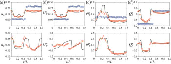


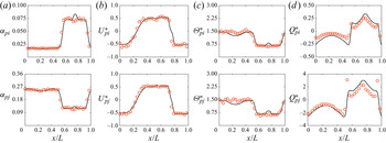


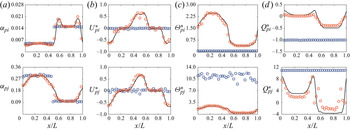


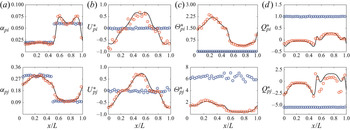


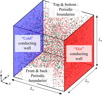


 Open access