


1. Introduction
Heavy oil reserves occupy approximately 70 % of whole oil reserves (Dusseault Reference Dusseault2001), but one of the major challenges with the use of heavy oil is its transport within a pipe because of its high viscosity. Among various drag reduction technologies investigated, water-lubricated transport has been known as an effective tool (Ghosh et al. Reference Ghosh, Mandal, Das and Das2009). This arrangement is called a core–annular flow because high viscosity oil is encapsulated in the pipe core region by less viscous water in the annulus. In experiments, core–annular flows in horizontal and vertical pipes have been considered, and drag reductions by water in the annulus have been observed in wide ranges of oil properties and flow conditions (Charles, Govier & Hodgson Reference Charles, Govier and Hodgson1961; Bai, Chen & Joseph Reference Bai, Chen and Joseph1992; Prada & Bannwart Reference Prada and Bannwart2001; Sotgia, Tartarini & Stalio Reference Sotgia, Tartarini and Stalio2008) and also validated in real-scale experiments with several-hundred-metre pipes (Arney et al. Reference Arney, Ribeiro, Guevara, Bai and Joseph1996; Rodriguez, Bannwart & de Carvalho Reference Rodriguez, Bannwart and de Carvalho2009). The differences in the flow characteristics between the vertical and horizontal pipes are attributed to different gravitational directions.
For a horizontal pipe, the directions of the main flow and gravity are perpendicular to each other and heavy oil rises by the buoyancy because the density of heavy oil is usually lower than that of water (Joseph et al. Reference Joseph, Bai, Chen and Renardy1997). The buoyancy force is balanced by the hydrodynamic (negative) lift force, which prevents the core from touching the wall and forms an eccentric core in the pipe. This lift force is caused by the pressure force from water lubrication at low Reynolds number (Ooms et al. Reference Ooms, Segal, van der Wees, Meerhoff and Oliemans1983) but is dominated by the inertial effect with increasing Reynolds number (Oliemans et al. Reference Oliemans, Ooms, Wu and Duijvestijn1987; Feng, Huang & Joseph Reference Feng, Huang and Joseph1995; Ooms, Pourquie & Poesio Reference Ooms, Pourquie and Poesio2012).
Many experimental studies have measured the variations of the pressure drop and oil holdup ( $\epsilon _o = V_o/V$, where $V_o$ and $V$ are the oil and whole pipe volumes, respectively) with the superficial velocities of oil and water for core–annular flows in horizontal pipes, and shown that the core–annular flow is effective in reducing the drag on the pipe wall (Charles et al. Reference Charles, Govier and Hodgson1961; Oliemans et al. Reference Oliemans, Ooms, Wu and Duijvestijn1987; Arney et al. Reference Arney, Bai, Guevara, Joseph and Liu1993; Sotgia et al. Reference Sotgia, Tartarini and Stalio2008; Vuong Reference Vuong2009; Shi, Gourma & Yeung Reference Shi, Gourma and Yeung2017; Tripathi et al. Reference Tripathi, Tabor, Singh and Bhattacharya2017). Vuong (Reference Vuong2009; $\mu _o = 0.23\unicode{x2013}1.07$ Pa s) and Shi (Reference Shi2015; $\mu _o = 3.3\unicode{x2013}7.1$ Pa s) showed that, when the oil viscosity ( $\mu _o$) is high enough, the pressure drop and flow pattern are not significantly changed by $\mu _o$ at high Reynolds numbers. Arney et al. (Reference Arney, Bai, Guevara, Joseph and Liu1993) observed that a core–annular flow with a non-Newtonian Bingham plastic oil (waxy crude oil/water emulsion: $\mu _o = 200\unicode{x2013}900$ Pa s) produces drag reduction but larger fluctuations in the pressure drop than that of the Newtonian oil (No. 6 fuel oil: $\mu _o = 2.7$ Pa s). Based on their own and other experimental data, Arney et al. (Reference Arney, Bai, Guevara, Joseph and Liu1993) suggested a pressure drop model based on the friction factor of single-phase pipe flow and an empirical holdup model, which was later modified by considering the eccentricity and oil fouling effects (Shi et al. Reference Shi, Gourma and Yeung2017). Other pressure drop and oil holdup models have been suggested from several studies (Oliemans, Pots & Trompe Reference Oliemans, Pots and Trompe1986; Brauner Reference Brauner1991; Bai et al. Reference Bai, Chen and Joseph1992; Bannwart Reference Bannwart2001; Kim & Choi Reference Kim and Choi2018).
Only a few studies have investigated the characteristics of turbulent core–annular flow in a horizontal pipe by experiments owing to the difficulty in flow measurements. Oliemans et al. (Reference Oliemans, Ooms, Wu and Duijvestijn1987) showed that turbulence effects are restricted near the lower surface of the pipe, and Tripathi et al. (Reference Tripathi, Tabor, Singh and Bhattacharya2017) observed a broad-banded spectrum of the phase interface wave. They demonstrated that large-wavelength interfacial modes dominate at low Reynolds numbers, while small-wavelength interfacial modes dominate at high Reynolds numbers. However, the dynamics of the phase interface, and the lift and drag forces on the core have been rarely investigated for the turbulent core–annular flow in a horizontal pipe. Thus, the detailed characteristics of turbulent flow and phase interface have been studied mostly by numerical simulations using interface tracking methods. For laminar flow, a few numerical simulations have been conducted to find the pressure distribution across the phase interface between oil and water. For example, Bai, Kelkar & Joseph (Reference Bai, Kelkar and Joseph1996) observed for axisymmetric laminar core–annular flows that the pressure difference across the phase interface between heavy oil and water increases as the gap size between the interface and pipe wall decreases, and thus suggested that an eccentric core–annular flow can be stably maintained because the gap size below the upper pipe wall is smaller (so, high pressure there) than that above the lower pipe wall (low pressure). This was confirmed by Ooms et al. (Reference Ooms, Pourquie and Poesio2012) for a laminar core–annular flow in a horizontal pipe using numerical simulation. They observed that, for a given wavy phase interface shape, the difference in the water pressures on the upper and lower interfaces increases with increasing eccentricity of the core and balances the buoyancy except at a very low Reynolds number where the direction of the lift force is the opposite to the gravitational direction.
For turbulent flow, studies have been limited to numerical simulations with turbulence models. For example, Shi et al. (Reference Shi, Gourma and Yeung2017) showed that the flow statistics change with turbulence models adopted, and a shear stress transport  $k-\omega$ turbulence model with turbulence damping at the phase interface works better than others. Their numerical results show a 30 % difference in the pressure drop and a 14 % difference in the holdup from those by experiments. Housz et al. (Reference Housz, Ooms, Henkes, Pourquie, Kidess and Radhakrishnan2017) showed using Launder–Sharma $k-\omega$ turbulence model that the difference in the pressure drops from experiment and numerical simulation is within 15 %, and their instantaneous amplitude and wavelength of the phase interface wave reasonably agree with those observed in experiments. So far, to the best of our knowledge, the only numerical simulation without using a turbulence model (i.e. direct numerical simulation) for turbulent core–annular flow is that by Kim & Choi (Reference Kim and Choi2018) in which the flow in a vertical pipe was considered. Li et al. (Reference Li, Pourquie, Ooms and Henkes2023) conducted Reynolds-Averaged Navier–Stokes simulation using the Launder–Sharma low-Reynolds number $k$-
$k$- $\epsilon$ model at the same condition considered by Kim & Choi (Reference Kim and Choi2018). Their simulation observed travelling interfacial waves like those of Kim & Choi (Reference Kim and Choi2018), but provided an 18 % lower friction factor and slightly higher holdup ratio.
As summarized above, the understanding of the flow characteristics in turbulent core–annular flow with water-lubricated high viscosity oil in a horizontal pipe is still very limited. Therefore, in the present study, we perform direct numerical simulation of this flow to investigate the asymmetric flow features inside the pipe and the pressure variation across the interface between oil and water. The spatiotemporal deformation of the phase interface is tracked with a level-set method. The details of numerical methods and flow conditions are given in § 2. In § 3, the axial pressure drop is compared with that of the experiment (Sotgia et al. Reference Sotgia, Tartarini and Stalio2008), and the characteristics of water flow in the annulus and high viscosity oil flow in the core are discussed, respectively. The spectral characteristics and dynamics of the phase interface are examined in §§ 4.1 and 4.2, respectively, followed by the investigation of near-wall flow dynamics in § 4.3. Finally, a summary is given in § 5.
2. Computational details
The numerical method to track the phase interface between two immiscible fluids, high viscosity oil and water, is essentially the same as that in our previous study on turbulent core–annular flow in a vertical pipe (Kim & Choi Reference Kim and Choi2018). We use a level-set method to track the interface (Herrmann Reference Herrmann2008; Kim & Moin Reference Kim and Moin2011),
 \begin{equation} \frac{\partial \phi}{\partial t} + u_j \frac{\partial \phi}{\partial x_j} = 0, \end{equation}
where  $x_j$ are the cylindrical coordinates, $u_j$ are the corresponding velocity components and $\phi$ is the level-set function which is a signed-distance function from the phase interface having positive values in water, negative ones in oil and zero at the phase interface. Equation (2.1) is solved at grids near the phase interface using a third-order total variation diminishing Runge–Kutta method in time (Gottlieb & Shu Reference Gottlieb and Shu1998) and a fifth-order weighted essentially non-oscillatory scheme in space in conjunction with a local Lax–Friedrichs entropy correction (Jiang & Peng Reference Jiang and Peng2000). A partial-differential-equation-based reinitialization method (Sussman, Smereka & Osher Reference Sussman, Smereka and Osher1994; Peng et al. Reference Peng, Merriman, Osher, Zhao and Kang1999) and a global mass conservation method (Son Reference Son2001; Zhang, Zou & Greaves Reference Zhang, Zou and Greaves2010) are used to preserve the signed-distance property, $|\boldsymbol {\nabla } \phi |= 1$, and compensate the volume loss, respectively. The periodic boundary condition is applied in the axial and azimuthal directions, and the Neumann boundary condition, $\partial \phi / \partial r = 0$, is used at the pipe wall.
The governing equations for unsteady incompressible two-phase flow are
 \begin{gather} \frac{\partial \rho u_i}{\partial t} + \frac{\partial \rho u_i u_j}{\partial x_j} =- \frac{{\rm d}P}{{\rm d}\kern0.06em x} \delta_{i1} - \frac{\partial p}{\partial x_i} + \frac{\partial}{\partial x_j} \left\{ \mu \left(\frac{\partial u_i}{\partial x_j} + \frac{\partial u_j}{\partial x_i} \right) \right\} - \rho g \delta_{i3} + \sigma \kappa \delta n_i, \end{gather}
 \begin{gather} \frac{\partial u_i}{\partial x_i} = 0, \end{gather}
where  $-{\rm d}P/{{\rm d}\kern0.7pt x}$ is the mean pressure gradient to drive a constant mass flow rate in a pipe, $p$ is the pressure fluctuation, $g$ is the gravitational acceleration, $\sigma$ is the surface tension coefficient, $\kappa$ is the curvature, $n_i$ is the surface-normal vector on the phase interface, $\delta _{ij}$ is the Kronecker delta, $i = 1$ and 3 for the streamwise (or axial) and vertical (the opposite direction to that of the gravity) directions, respectively, and $\delta$ is the delta function (non-zero value at the phase interface and zero otherwise). The density and viscosity are constants for each fluid, but change continuously near the phase interface like
 \begin{gather} \rho = \rho_o + (\rho_w - \rho_o) \psi, \end{gather}
 \begin{gather} \mu = \mu_o + (\mu_w - \mu_o) \psi, \end{gather}
where the subscripts  $w$ and $o$ denote water and oil, respectively. Here, $\psi$ is the water volume fraction in a control volume calculated from the linearization of the level-set function (van der Pijl et al. Reference van der Pijl, Segal, Vuik and Wesseling2005; Herrmann Reference Herrmann2008). Thus, $\psi = 0$ or 1 for the cells containing oil or water only, respectively, and $0 < \psi < 1$ for the cells containing the phase interface. The density and viscosity of oil used for present simulations are $\rho _o = 889\ {\rm kg}\ {\rm m}^{-3}$ and $\mu _o = 0.919$ Pa s, and those of water are $\rho _w = 998\ {\rm kg}\ {\rm m}^{-3}$ and $\mu _w = 0.001$ Pa s, respectively, and the surface tension coefficient is $\sigma = 0.02\ {\rm N}\ {\rm m}^{-1}$ (Sotgia et al. Reference Sotgia, Tartarini and Stalio2008). We also confirmed that oil used in the experiment was Newtonian (G. Sotgia, private communication).
Equations (2.2) and (2.3) are solved using a four-step fractional step method (Choi & Moin Reference Choi and Moin1994),
 $$\begin{gather} \frac{\hat{\rho} \hat u_i - \rho^n u_i^n}{\Delta t} + \frac{1}{2} \frac{\partial}{\partial x_j} \left(\hat{\rho} \hat u_i \hat u_j + \rho^n u_i^n u_j^n \right) =- \frac{{\rm d}P^n}{{\rm d}\kern0.7pt x} \delta_{i1} - \frac{\partial p^n}{\partial x_i}\nonumber\\ + \frac{1}{2}\frac{\partial}{\partial x_j} \left\{ \hat{\mu} \left(\frac{\partial \hat u_i}{\partial x_j} + \frac{\partial \hat u_j}{\partial x_i} \right) + \mu^n \left(\frac{\partial u^n_i}{\partial x_j} + \frac{\partial u^n_j}{\partial x_i} \right)\right\} -\frac{1}{2} \left( \hat{\rho} + \rho^n \right) g \delta_{i3} + \sigma \kappa^n \delta^n n_i^n, \end{gather}$$
 $$\begin{gather}\frac{\hat{\rho} u_i^\ast- \hat{\rho} \hat u_i}{\Delta t} = \frac{\partial p^n}{\partial x_i}, \end{gather}$$
 $$\begin{gather}\frac{\partial}{\partial x_i} \left( \frac{1}{\hat{\rho}} \frac{\partial p^{n+1}}{\partial x_i} \right) = \frac{1}{\Delta t} \frac{\partial u_i^\ast}{\partial x_i}, \end{gather}$$
 $$\begin{gather}\frac{\hat{\rho} u_i^{n+1} - \hat{\rho} u_i^\ast}{\Delta t} =- \frac{\partial p^{n+1}}{\partial x_i}, \end{gather}$$
where  $\hat {\rho }$ and $\hat {\mu }$ are the provisional density and viscosity obtained from (2.4), (2.5) and the continuity equation, ${\partial \rho }/{\partial t} + {\partial \rho u_j}/{\partial x_j} = 0$ (see Kim & Choi (Reference Kim and Choi2018) for the detail), $\Delta t$ is the computational time step size, and the superscript $n$ is the time step index. The second-order central difference scheme is used for all the spatial derivative terms except the convection term near the phase interface where an upwind-type mass-flux scheme is applied (Kim & Moin Reference Kim and Moin2011; Raessi & Pitsch Reference Raessi and Pitsch2012). The Crank–Nicolson method is applied to the convection and diffusion terms to avoid severe time step restriction. To solve the resulting system matrix, a Newton iterative method with an approximate factorization (Choi, Moin & Kim Reference Choi, Moin and Kim1993) and an Aitken-type accelerator (Irons & Tuck Reference Irons and Tuck1969) are adopted. The surface tension term is explicitly treated with a continuum surface force approach (Brackbill, Kothe & Zemach Reference Brackbill, Kothe and Zemach1992). An iterative constant-coefficient Poisson solver (Kim & Moin Reference Kim and Moin2011) using a fast Fourier transform is applied to solve the variable-coefficient pressure Poisson equation (2.8). The details of numerical methods are available in Kim & Choi (Reference Kim and Choi2018).
Figure 1 shows the schematic diagram of a core–annular flow in a horizontal pipe. The gravity direction is perpendicular to the mean flow direction, and thus the oil core naturally rises by the buoyancy due to its lower density than that of water. The cylindrical coordinates  $(x, r, \theta )$ and the corresponding velocity components $(u, v, w)$ are used for simulation, and the $y$ and $z$ coordinates are used for convenience to represent the lateral and vertical directions at the pipe cross-section, respectively. We fix the superficial velocity of oil, $j_o = q_o/{\rm \pi} R^2 = 0.88\ {\rm m}\ {\rm s}^{-1}$, and vary the superficial velocity of water as $j_w = q_w/{\rm \pi} R^2 = 0.05, 0.075, 0.1, 0.15, 0.22$ and $0.36\ {\rm m}\ {\rm s}^{-1}$, where ${R (= 0.013\,{\rm m})}$ is the pipe radius, and $q_o$ and $q_w$ are the volume flow rates of oil and water, respectively. This is one of the experimental conditions in Sotgia et al. (Reference Sotgia, Tartarini and Stalio2008), where a core–annular flow is maintained in the pipe. Note that Sotgia et al. (Reference Sotgia, Tartarini and Stalio2008) varied the oil and water superficial velocities together with the pipe radius and showed various flow regimes including core–annular and dispersed flows. The numerical method of maintaining constant superficial velocities of both fluids is given in Appendix A.

Figure 1. Schematic diagram of the core–annular flow in a horizontal pipe.
Table 1 shows the bulk Reynolds number,  $Re_b = u_b(2R)/\nu _w = (j_w+j_o)(2R)/\nu _w$, number of grid points, computed friction Reynolds number, $Re_\tau = u_\tau R/\nu _w$, and oil holdup, $\epsilon _o = V_o / V$, for six superficial velocity ratios, $j_w/j_o$. Here, $V$ is the total computational volume, $V_o$ is the volume occupied by oil, $u_\tau = \sqrt {\bar {\tau }_w / \rho _w}$ is the friction velocity, $\bar {\tau }_w$ is the mean wall shear stress and $\nu _w$ is the kinematic viscosity of water. For comparison, we also conduct a numerical simulation of water flow at a similar Reynolds number ( $Re_b = 24\,580$), whose results agree well with those of Wu & Moin (Reference Wu and Moin2008). The streamwise domain size ( $L_x$) is $2 {\rm \pi}R$ except that of single-phase flow simulation ( $10R$), and periodic boundary conditions are applied in the streamwise ( $x$) and azimuthal ( $\theta$) directions where uniform grids are used. As shown in § 3, large-scale structures in the core–annular flow are confined by the wavelength of the phase interface, and thus the streamwise domain size of $L_x = 2{\rm \pi} R$ is large enough to contain those structures for the cases considered. The no-slip boundary condition is used at the wall, and in the radial ( $r$) direction dense grids are allocated near the wall and interface, but coarse grids are used in the core region where flow is laminar due to the high viscosity of oil. Grid resolutions in wall units are $\Delta x^+ = \Delta x u_\tau / \nu _w \approx 6\unicode{x2013}7, \Delta r^+_{min} \approx 0.6\unicode{x2013}0.7$ and $(R \Delta \theta )^+ \approx 6\unicode{x2013}7$. The number of grid points used for the level-set equation is twice that for the Navier–Stokes equation in each direction. We simulated flow with one and half times the grid points for the streamwise and azimuthal directions for the case of $j_w/j_o = 0.17$, and the result showed the changes in the pressure drop and oil holdup less than 4 % and 1 %, respectively. All the computations are carried out for the non-dimensional time of approximately $250 R/j_o$, and averaging is conducted over $150 R/j_o$ to obtain mean values.
Table 1. Superficial velocity ratio, bulk Reynolds number, number of grid points, computed friction Reynolds number and oil holdup.

3. Characteristics of the core and annular flows
Figure 2 shows the variation of the mean pressure gradient with the superficial velocity ratio for a fixed superficial oil velocity ( $\,j_o = q_o/{\rm \pi} R^2 = 0.88\ {\rm m}\ {\rm s}^{-1}$), together with the experimental result by Sotgia et al. (Reference Sotgia, Tartarini and Stalio2008). An excellent agreement between the present and experimental data is observed for $j_w/j_o \ge 0.17$, but the agreement becomes poorer at lower $j_w/j_o$. This relative disagreement at low $j_w/j_o$ may be attributed to the fact that oil frequently sticks to the wall due to a narrow water region (Bai et al. Reference Bai, Chen and Joseph1992; Arney et al. Reference Arney, Bai, Guevara, Joseph and Liu1993), which may change the relative location of the phase interface and thus the mean pressure drop (note that the present numerical method does not prevent the formation of oil drops or oil sticking to the wall, but such phenomena do not occur during the present simulations). A similar discrepancy at low $j_w/j_o$ was also observed for turbulent core–annular flow in a vertical pipe (Kim & Choi Reference Kim and Choi2018). With increasing $j_w/j_o$, the mean pressure gradient first decreases, reaches a minimum and then increases, providing an optimal superficial velocity of water ( $\,j_w \vert _{opt}$) for the lowest mean pressure gradient to transport a given oil flow rate ( $q_o$ or $j_o$) in a pipe. This has also been observed in other experiments of core–annular flows in vertical and horizontal pipes (Bai et al. Reference Bai, Chen and Joseph1992; Prada & Bannwart Reference Prada and Bannwart2001; Sotgia et al. Reference Sotgia, Tartarini and Stalio2008; Vuong Reference Vuong2009; Housz et al. Reference Housz, Ooms, Henkes, Pourquie, Kidess and Radhakrishnan2017). The optimal superficial velocity ratios obtained from present numerical simulation and experiment by Sotgia et al. (Reference Sotgia, Tartarini and Stalio2008) are slightly different ( $\,j_w/j_o \vert _{opt} = 0.11$ and 0.085, respectively), because flow conditions are not exactly same due to non-hydrodynamic effects such as chemical adhesion (Arney et al. Reference Arney, Ribeiro, Guevara, Bai and Joseph1996) as described before. When $j_w/j_o$ is smaller than the optimal one, the mean pressure gradient increases because of high wall shear stress from the narrow gap between the phase interface and upper wall (for $j_w/j_o=0.057$, the minimum gap size is $8$ wall units, where 9 and 18 grid points for the Navier–Stokes and level-set equations are located). On the other hand, when $j_w/j_o$ is larger than the optimal one, the pressure gradient increases again because of the increase in the bulk Reynolds number, $Re_b = (j_w+j_o)(2R)/\nu _w$. For large superficial velocity ratios, the corresponding water flows are similar to single-phase flows (see later in figure 6c), and thus the mean pressure gradient follows the Blasius friction factor formula, $ (-{{\rm d}P}/{{\rm d}\kern0.7pt x}) ({R}/{\rho _w u_b^2}) \sim Re_b^{-1/4}$, where $u_b = j_w + j_o$. Since $Re_b^{-1/4}$ little changes in the range of the Reynolds numbers considered (see table 1), the mean pressure gradient normalized by $j_o^2$ increases with increasing $j_w/j_o$ for $j_w/j_o \ge 0.17$ (figure 2), i.e.
 \begin{equation} - \frac{{\rm d}P}{{\rm d}\kern0.7pt x} \frac{R}{\rho_w j_o^2} =-\frac{{\rm d}P}{{\rm d}\kern0.7pt x} \frac{R}{\rho_w u_b^2} \left(1 + \frac{j_w}{j_o}\right)^2 \sim \left(1 + \frac{j_w}{j_o}\right)^2. \end{equation}
The mean pressure gradient of the core–annular flow normalized by  $\rho _w$ and $u_b (= j_o+j_w)$ is $(-{\rm d}P/{{\rm d}\kern0.06em x}) (R / \rho _w u_b^2) = 8 Re_\tau ^2 / Re_b^2$ (from momentum analysis) $\approx 0.0067$ at $j_w/j_o = 0.085\ (Re_b = 24\,780)$, which is similar to 0.0064 obtained for the single-phase water flow at $Re_b = 24\,580$, and is much lower than $(-{\rm d}P/{{\rm d}\kern0.7pt x}) (R / \rho _w u_b^2) = (16 / Re_b) (\rho _o/\rho _w) \approx 0.64$ for single-phase high-viscosity laminar oil flow ( $u_b = j_o = 0.88\ {\rm m}\ {\rm s}^{-1}$; $Re_b = 22.13$; normalized by $\rho _w$ for comparison). This clearly indicates that the core–annular flow significantly reduces the drag for the heavy-oil delivery.

Figure 2. Variation of the mean pressure gradient with the superficial velocity ratio:  $\bullet$, present simulation; $\circ$, experiment by Sotgia et al. (Reference Sotgia, Tartarini and Stalio2008).
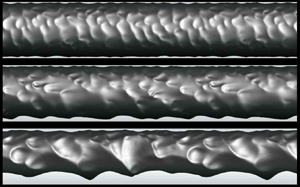
Figure 3 shows the shapes of the instantaneous phase interface for different superficial velocity ratios, together with snapshots of the phase interface from experiment by Sotgia et al. (Reference Sotgia, Tartarini and Stalio2008). Also shown in figure 3(a–f) are the contours of the instantaneous relative velocity to the core velocity in water flow, where  $u_{core} = \int u\,{\rm d}V_o / V_o =\int u \,{\rm d}V_o/V {\times } (V/V_o) = j_o / \epsilon _o$ and $V_o$ is the volume occupied by oil. The shapes of the phase interface qualitatively agree well with the experimental ones considering the differences in the experimental and simulation set-ups as mentioned above. Due to the buoyancy, the flow characteristics vary in the azimuthal direction. The lower gap between the phase interface and pipe wall rapidly increases with increasing superficial velocity ratio, whereas the upper gap slowly increases (see below). The phase interfaces consist of different streamwise and azimuthal wavenumber components, and the wavelength and wave amplitude increase with increasing superficial velocity ratio (or increasing gap size). When the gap is narrow, the crest of the phase interface almost touches the wall, and no small-scale vortices are observed there (see later in figure 5a). With increasing $j_w/j_o$, the flow in the gap changes from laminar to turbulent, especially near the lower pipe wall.

Figure 3. Shapes of the instantaneous phase interface and contours of the instantaneous relative velocity to the core velocity for different superficial velocity ratios: (a)  $j_w/j_o = 0.057$; (b) 0.085; (c) 0.11; (d) 0.17; (e) 0.25; (f) 0.41; (g) 0.057; (h) 0.41. Here, (a–f) are from the present numerical simulation and (g,h) are from the experiment by Sotgia et al. (Reference Sotgia, Tartarini and Stalio2008).
Figure 4(a) shows the mean radial locations of the phase interface in the azimuthal direction for different superficial velocity ratios,
 \begin{equation} \tilde{h} (\theta) = \frac{1}{L_x T} \int^T_0 \int^{L_x}_0 h\, {{\rm d}\kern0.7pt x}\, {\rm d}t, \end{equation}
where  $h$ is the instantaneous radial location of the phase interface, the superscript $\tilde {.}$ denotes the averaging over the streamwise direction and in time, and $T$ is the integration time. The averaged value of $\tilde {h}(\theta )$ over the azimuthal direction is $h_{avg} / R = \sqrt {V_o / V} = \sqrt {\epsilon _o}$, and they are $h_{avg} / R = 0.96, 0.94, 0.93, 0.90, 0.87$ and 0.81 for $j_w/j_o = 0.057, 0.085, 0.11, 0.17, 0.25$ and 0.41, respectively. For $j_w/j_o = 0.057$, $\tilde {h} (\theta )$ is nearly constant in the azimuthal direction due to the small amount of water flow, but, for higher $j_w/j_o$, it has a plateau near the top wall ( $\theta \approx 0^{\circ }$) but rapidly decreases near the bottom wall ( $\theta \approx 180^{\circ }$) because the core rises upward by the buoyancy. The gap size between the phase interface and wall, $R - \tilde {h}(\theta )$, increases with $j_w/j_o$ for all azimuthal locations (figure 4b). At large superficial velocity ratios, the gap size increases almost linearly with the superficial velocity ratio. This linear growth in the gap size starts to occur at lower superficial velocity ratio for larger $\theta$.

Figure 4. Mean radial locations of the phase interface and mean gap sizes along the azimuthal direction for different superficial velocity ratios: (a) mean radial location,  $\tilde {h} (\theta )$; (b) mean gap size, $R - \tilde {h} (\theta )$. Here, $\theta = 0^{\circ }$ and $180^{\circ }$ denote the top and bottom locations of the pipe, respectively.
Figure 5 shows the contours of the instantaneous modified pressure fluctuations,  $p^\ast (=p + \rho _w gz - \bar {p}^\ast _{wall})$, and the instantaneous velocity vectors relative to the core velocity for $j_w/j_o = 0.057$ and 0.41, where $\bar {p}_{wall}^\ast = \int (p+\rho _w g z) \,{\rm d}A_{wall} / A_{wall}$ and $A_{wall}$ is the area of the pipe wall. Here, we add $\rho _w g z$ in the modified pressure to remove the hydrostatic effect in the pressure. For the narrow gap of $j_w/j_o = 0.057$, there is a recirculating flow in the wave valley, and high- and low-pressure fluctuations are observed ahead of and behind the crest, which is similar to those observed from core–annular flows in vertical pipes (Bai et al. Reference Bai, Kelkar and Joseph1996; Li & Renardy Reference Li and Renardy1999; Kim & Choi Reference Kim and Choi2018). However, for $j_w/j_o = 0.41$, the gap between the interface and lower pipe wall is sufficiently wide and turbulent flow is observed within an oil-free region near the lower wall. Near the crest, $p^\ast$ is high and low ahead of and behind the crest, respectively. This indicates that the oil flow in the core drags the water flow. Also, $p^\ast$ is overall high and low near the upper and lower surfaces of the pipe, respectively, and this difference is in balance with the buoyancy (Feng et al. Reference Feng, Huang and Joseph1995; Ooms et al. Reference Ooms, Pourquie and Poesio2012), which is discussed later in § 4.2.

Figure 5. Contours of the instantaneous modified pressure fluctuations and relative velocity vectors: (a)  $j_w/j_o = 0.057$; (b) 0.41. The velocity vectors relative to the core velocity are drawn at every eighth grid points in the streamwise and radial directions, except for the zoomed view in (a) where they are drawn at every other grid point.
Figure 6 shows the mean streamwise velocity profiles of water ( $\tilde {u}_w$) and oil ( $\tilde {u}_o$) normalized by the core velocity $u_{core}$ and local friction velocity $\tilde {u}_\tau (\theta )$, respectively, for $j_w/j_o = 0.057, 0.17$ and 0.41, where $\tilde {u}_w, \tilde {u}_o$ and $\tilde {u}_\tau$ are obtained as
 \begin{gather} \tilde{u}_w (r, \theta) = \frac{\displaystyle\int^T_0 \int^{L_x}_0 u(x, r, \theta, t) \psi(x, r, \theta, t) \,{{\rm d}\kern0.7pt x}\, {\rm d}t}{\displaystyle\int^T_0 \int^{L_x}_0 \psi(x, r, \theta, t) \,{\rm d}\kern0.06em x\,{\rm d}t}, \end{gather}
 \begin{gather} \tilde{u}_0 (r, \theta) = \frac{\displaystyle\int^T_0 \int^{L_x}_0 u(x, r, \theta, t) (1 - \psi(x, r, \theta, t)) \,{{\rm d}\kern0.7pt x}\, {\rm d}t}{\displaystyle\int^T_0 \int^{L_x}_0 (1 - \psi(x, r, \theta, t)) \,{\rm d}\kern0.06em x\,{\rm d}t}, \end{gather}
 \begin{gather} \tilde{u}_\tau (\theta) = \sqrt{\nu_w \int^T_0 \int^{L_x}_0 \left( -\partial u / \partial r \vert_{wall} \right) \,{\rm d}\kern0.06em x\,{\rm d}t / (L_x T)}. \end{gather}
Since the core flow is almost a plug flow,  $\tilde {u}_o/u_{core} \approx 1$ but slightly decreases with increasing $r$. The annular flow may be considered as a Poiseuille–Couette-type flow driven by both the mean pressure gradient and the core. For $j_w/j_o = 0.057$ (figure 6a), the gap between the interface and wall is narrow and little varies along the azimuthal direction (see figure 4). Thus, $\tilde {u}_w$ at different azimuthal locations are quite similar among themselves and have linear profiles except near the interface, indicating that the flow in water at this low superficial velocity ratio is more like Couette flow driven by the core. With increasing $j_w/j_o$, the gap size increases and the water velocity profile approaches the log-law of the single-phase flow (see the velocity profiles at $\theta = 180^{\circ }$ for $j_w/j_o = 0.17$ and at $\theta = 90^{\circ }$ and $180^{\circ }$ for $j_w/j_o = 0.41$ in figures 6b and 6c, respectively). Note that the oil-free region at $\theta =180^\circ$ becomes wider with increasing $j_w / j_o$ and the mean velocity profiles there follow the law of the wall of the single-phase flow.

Figure 6. Profiles of the mean streamwise velocity of water ( $\tilde {u}_w$) and oil ( $\tilde {u}_o$) normalized by (a i,b i,c i) $u_{core}$ and (aii, bii, cii) local friction velocity $\tilde {u}_\tau (\theta )$ , respectively: (a) $j_w/j_o = 0.057$; (b) 0.17; (c) 0.41.
Figure 7(a) shows the variations of the mean core-flow characteristics including the holdup ratio ( $s = (q_o/q_w)/(V_o/V_w)$), oil holdup ( $\epsilon _o = V_o/(V_w+V_o)$) and core ( $u_{core}$) and annular ( $u_{annular}$) velocities with $j_w/j_o$. The holdup ratio is the ratio of the bulk velocity of oil (core) to that of water (annular) and is greater than 1, because the annular water flow is heavily influenced by the viscous effect. With increasing $j_w/j_o$, the holdup ratio decreases from 1.50 to 1.29, indicating that the amount of increase in $V_w/V_o$ is smaller than that in $j_w/j_o (= q_w/q_o)$. With increasing $j_w/j_o$, the oil holdup $\epsilon _o$ decreases, and the core and annular velocities normalized by $j_o (u_{core}/j_o = 1/\epsilon _o)$ increase.

Figure 7. Mean characteristics of the core flow: (a) holdup ratio ( $s$), oil holdup ( $\epsilon _o$), core velocity ( $u_{core}/j_o$) and annular velocity ( $u_{annular}/j_o$); (b) contours of the mean water volume fraction $\tilde {\psi }$ (black solid line) and the mean location of the phase interface $\tilde {h} (\theta )$ (red solid line) for $j_w/j_o = 0.41$; (c) eccentricity ( $e$) and roundness ( $\chi$). Contour levels of $\tilde {\psi }$ are from 0.05 to 0.95 by increments of 0.1.
Figure 7(b) shows the contours of the mean water volume fraction  $\tilde {\psi } (r, \theta )$ and the mean location of the phase interface $\tilde {h}(\theta )$ for $j_w/j_o = 0.41$, where $\tilde {\psi }(r,\theta ) = \int ^T_0 \int ^{L_x}_0 \psi (x,r,\theta,t)\,{\rm d}\kern0.06em x\,{\rm d}t / (L_x T)$. The region of $0 < \tilde {\psi } < 1$ is wider near the lower pipe wall than that near the upper one, which indicates that the amplitude of the phase interface wave is large and small near the lower and upper pipe walls, respectively. As shown with $\tilde {h}(\theta )$, the core is deformed due to the buoyancy and is eccentric to the pipe centre. Figure 7(c) shows the roundness $\chi$ and eccentricity $e$ of the phase interface. The roundness $\chi$ is defined as (the ratio of the volume of the core to that of a circular cylinder having the same surface area of the core)
 \begin{equation} \chi = 4 {\rm \pi}\frac{\displaystyle\int^T_0 \int^{L_x}_0 \int^{2{\rm \pi}}_0 \dfrac{1}{2} h^2 \,{\rm d}\theta \,{\rm d}\kern0.06em x\,{\rm d}t / (L_x T)}{\left\{\displaystyle\int^T_0 \int^{L_x}_0 \int^{2{\rm \pi}}_0 h \,{\rm d}\theta \,{\rm d}\kern0.06em x\,{\rm d}t / (L_x T)\right\}^2}, \end{equation}
and the eccentricity is  $e = z_{cm} / (R - h_{avg})$, where $z_{cm} (= \int ^T_0 \int ^V_0 z (1 - \psi ) \,{\rm d}V\,{\rm d}t / \int ^T_0 \int ^V_0 (1-\psi ) \,{\rm d}V\,{\rm d}t)$ is the vertical distance from the pipe centre to the centre of mass of the core, and $h_{avg} = \int ^{2{\rm \pi} }_0 \tilde {h} (\theta ) \,{\rm d}\theta / 2 {\rm \pi}$ is the overall mean radius of the phase interface. To calculate the perimeter $\int h \,{\rm d}\theta$, the trapezoidal rule is used. The roundness of the circle is 1, but that of the core is less than 1 and decreases with increasing $j_w/j_o$. For $j_w/j_o = 0.41$, the interface is most deformed among the cases considered and the roundness is approximately 0.94, which is similar to that of the ellipse whose major and minor axes are 1.5 and 1, respectively. Instantaneous interface shapes are much more non-circular than the mean shape shown in figure 7(b). The eccentricity is very small for $j_w/j_o = 0.057$, indicating that the phase interface is nearly circular because oil occupies almost the whole circular pipe. The eccentricity rapidly increases from $j_w/j_o = 0.057$ to 0.085, is nearly constant for $0.085 < j_w/j_o < 0.25$ and then slowly increases with increasing $j_w/j_o$, because the core rises upward.
4. Phase interface and near-wall dynamics
4.1. Wave characteristics of the phase interface
The wave characteristics of the phase interface are investigated by computing the streamwise wavenumber ( $k_x$) and frequency ( $\omega$) power spectra of the phase interface amplitude, $\zeta (\theta ) (= h - \tilde {h}(\theta ))$. The range of the streamwise wavenumber is $0 \le k_x \le 383/R$ $(\Delta k_x = 1/R)$, and the sampling interval is $\Delta t_s = 0.02 R/j_o$ during $T = 81.92 R/j_o$ which is divided into 15 overlapping segments with 50 % overlap ( $0 \le \omega \le 157 j_o/R$ with $\Delta \omega = 0.6136 j_o/R$; for more details, see Choi & Moin (Reference Choi and Moin1990)). The one-dimensional wavenumber spectrum $\varphi (k_x,\theta )$ and frequency spectrum $\varphi (\omega,\theta )$ of the phase interface amplitude $\zeta$ satisfy the following condition:
 \begin{equation} \int^\infty_0 \varphi (k_x,\theta) \,{\rm d}k_x = \int^\infty_0 \varphi(\omega,\theta) \,{\rm d}\omega = \zeta^2_{rms} (\theta), \end{equation}
where  $\zeta _{rms}(\theta )$ is the root-mean-square fluctuations of the phase interface amplitude.
Figure 8 shows the streamwise wavenumber and frequency spectra of the phase interface amplitude at  $\theta = 0^\circ$ and $180^\circ$ for $j_w/j_o = 0.057, 0.17$ and 0.41. The spectra are broad-banded, indicating that the motion of the phase interface amplitude has a turbulent nature. For $j_w/j_o = 0.057$, the streamwise wavenumber spectrum is more or less homogeneous in the azimuthal direction, and high powers appear in low wavenumbers, $k_x R \le 12$ $(\lambda \ge {\rm \pi}R/6)$, where $\lambda$ is the corresponding wavelength. With increasing $j_w/j_o$, the power peak moves to lower wavenumbers on the bottom interface ( $\theta = 180^{\circ }$), whereas the power on the top interface is relatively insensitive to $j_w/j_o$. This is consistent with the variation of large-scale wavy structures on the bottom interface with $j_w/j_o$ in figure 3: the power peak occurs at $k_x R = 12, 5$ and 3 for $j_w/j_o = 0.057, 0.17$ and 0.41, respectively, corresponding to the dominant wavelengths of $\lambda /R = 0.52, 1.26$ and $2.09$. Note also that the power at low wavenumbers and frequencies is much larger at $\theta = 180^{\circ }$ than at $\theta = 0^{\circ }$ for $j_w/j_o = 0.17$ and 0.41. The frequency spectra are very similar to the streamwise wavenumber spectra, showing the convective nature of the phase interface.

Figure 8. Streamwise wavenumber and frequency spectra of the phase interface amplitude at  $\theta =0^{\circ }$ and $180^{\circ }$: (a) $j_w/j_o = 0.057$; (b) 0.17; (c) 0.41.
Figure 9(a) shows the contours of the streamwise wavenumber–frequency power spectrum of the phase interface amplitude,  $\varPhi (k_x,\omega ) = \int ^{2{\rm \pi} }_0 \tilde {\varPhi }(k_x,\omega,\theta ) \,{\rm d}\theta / 2{\rm \pi}$, for $j_w/j_o = 0.17$, where $\tilde {\varPhi }(k_x,\omega,\theta )$ is the two-dimensional power spectrum as a function of the azimuthal angle. As shown, the streamwise wavenumber–frequency power spectrum shows a strong convective nature. The convection velocity of the phase interface can be obtained as (Wills Reference Wills1971; Choi & Moin Reference Choi and Moin1990)
 \begin{equation} \tilde{U}_{conv} (k_x, \theta) =- \frac{\omega (k_x,\theta)}{k_x}, \end{equation}
where  $\omega (k_x,\theta )$ is obtained from
 \begin{equation} \left.\frac{\partial \tilde{\varPhi}(k_x,\omega,\theta)}{\partial \omega} \right\vert_{\omega = \omega(k_x,\theta)} = 0. \end{equation}
A quadratic polynomial is used to find  $\omega (k_x,\theta )$ in (4.3) (Kang, Moin & Iaccarino Reference Kang, Moin and Iaccarino2008). Figure 9(b) shows the convection velocity normalized by the core velocity as a function of the streamwise wavenumbers at three different azimuthal angles. The scatters of the data shown in this figure are due to the limited statistical sample available for locating the maxima of the spectrum within a set of discrete frequencies and wavenumbers, and the convection velocities at low wavenumbers are also contaminated by a specific window function (Hanning window) or the sampling period used (see also Choi & Moin (Reference Choi and Moin1990) and Kim & Choi (Reference Kim and Choi2018)). The convection velocity is smaller than the core velocity, indicating that the core drags the phase interface. At low wavenumbers where the spectrum has a peak ( $k_x R = 1\unicode{x2013}10$), the convection velocities are lower than those at higher wavenumbers ( $\tilde {U}_{conv} (k_x,\theta ) / u_{core} \approx 0.94\unicode{x2013}0.98$), suggesting that the energy-containing large-scale structures of the phase interface more strongly interact with the water flow and resist the core flow more than the small-scale structures do. This characteristic is similar to that of the core–annular flow in a vertical pipe (Kim & Choi Reference Kim and Choi2018). Note also that the convection velocity at $\theta =0^{\circ }$ is lower than those at $\theta =90^{\circ }$ and $180^{\circ }$ due to the viscous effect at the narrow gap, although the difference is not so large. The overall convection velocity $U_{conv}$ of the most energetic wave is obtained from
 \begin{equation} \left.\frac{\partial W(U^\ast)}{\partial U^\ast} \right\vert_{U^\ast= U_{conv}} = 0, \end{equation}
where
 \begin{equation} W(U^\ast) = \int \varPhi (k_x, -U^\ast k_x) \,{\rm d}k_x. \end{equation}
The overall convection velocity increases with increasing  $j_w/j_o$; i.e. $U_{conv}/u_{core} \approx 0.94, 0.95$ and 0.96 for $j_w/j_o = 0.057, 0.17$ and 0.41, respectively. This indicates that most energetic motions move downstream at a speed slightly lower than the core velocity.

Figure 9. Two-dimensional spectrum and convection velocity of the phase interface ( $\,j_w/j_o = 0.17$): (a) contours of $\varPhi (k_x,\omega )$; (b) convection velocity at three different azimuthal locations as a function of the streamwise wavenumber. In (a), contour levels are logarithmically equally spaced.
4.2. Dynamics of oil core
The stress on the phase interface is obtained as
 \begin{equation} \sigma_{ij} n_j = \left\{-p \delta_{ij} + \mu \left( \frac{\partial u_i}{\partial x_j} + \frac{\partial u_j}{\partial x_i} \right) \right\} n_j, \end{equation}
where the subscripts  $i = 1, 2$ and 3 indicate the axial ( $x$), lateral ( $y$) and vertical ( $z$) coordinates, respectively (figure 1). The pressure and velocity gradient on the interface are obtained by a linear interpolation from grid points at the nearest oil region to those at the phase interface. From the stress boundary condition at the phase interface ( jump condition), the stress at the phase interface from the core region is the sum of the stress at the phase interface from the annular region and the surface tension (Brackbill et al. Reference Brackbill, Kothe and Zemach1992).
Figure 10 shows the contours of the instantaneous stresses on the interface,  $\sigma _{zj} n_j / (\rho _w - \rho _o)gR$ and $\sigma _{xj} n_j / \rho _w u_\tau ^2$, and their components for $j_w/j_o = 0.41$. Here, the viscous normal stress is included in the pressure. Note that the stresses $\sigma _{zj}$ and $\sigma _{xj}$ are normalized by the hydrostatic pressure difference and wall shear stress, respectively, to explain $\sigma _{zj}$ and $\sigma _{xj}$ in terms of the lift and drag forces, respectively. The stagnation pressure ahead of the crest generates the wall-repulsive ( $-r$ direction) and drag ( $-x$ direction) forces (in this figure, $\delta _{xj} n_j$ are positive and negative on the forward and leeward sides, respectively). The pressure on the upper interface is higher than that of the lower one ( $\delta _{zj} n_j$ are positive and negative on the upper and lower interfaces, respectively), providing a negative lift ( $-z$ direction) force on the core which balances its buoyancy force, whereas the contribution of the viscous shear stress to the lift force is very small (figure 10a). For the drag force (figure 10b), both the pressure and viscous shear stress are highly positive and negative on the forward side of the crest, respectively, and thus push the crest in the upstream direction, whereas low pressure and positive viscous shear stress are generated on the leeward side of the crest, indicating that the flow separates across the crest.

Figure 10. Contours of the instantaneous stresses acting on the phase interface ( $\,j_w/j_o = 0.41$): (a) $\sigma _{zj} n_j / (\rho _w - \rho _o)gR$; (b) $\sigma _{xj} n_j / \rho _w u_\tau ^2$.
Figure 11 shows the variations of the mean lift ( $C_L = - \bar {F}_z / (\rho _w-\rho _o)gV_o$) and drag ( $C_D = - \bar {F}_x / \rho _w u_\tau ^2 A_{core}$) coefficients on the oil core with $j_w/j_o$, together with the analytic solutions of the mean lift and drag coefficients ( $C_L = 1$ and $C_D = \sqrt {\epsilon _0 \chi }$), where the instantaneous forces are obtained by integrating the stresses over the phase interface,
 \begin{equation} F_i = \int \sigma_{ij} n_j \,{\rm d}A = \int \left\{-p \delta_{ij} + \mu \left( \frac{\partial u_i}{\partial x_j} + \frac{\partial u_j}{\partial x_i} \right) \right\} n_j \,{\rm d}A, \end{equation}
and  $A_{core}$ is the surface area of the phase interface at the same oil holdup. The analytical mean drag coefficient of $C_D=\sqrt {\epsilon _o \chi }$ is obtained by combining the momentum balances on the whole domain and oil core, respectively, and introducing $\chi = 4 {\rm \pi}A_o / \mathcal {P}^2$, $\epsilon _o = V_o/V = A_o/{\rm \pi} R^2$ and $A_{core}=\mathcal {P} L_x$, where $A_o$ is the cross-sectional area of the oil core, and $\mathcal {P}$ is the wetted perimeter of the phase interface (see Appendix B for the derivation). As shown in this figure, the computations of $C_L$ and $C_D$ on the phase interface using (4.7) are not very accurate but contain maximum 10 % errors because the surface tension force is smeared out from the phase interface by using the continuum surface force approach (Brackbill et al. Reference Brackbill, Kothe and Zemach1992). As discussed in figure 10(a), the contribution of the pressure to the lift is dominant and that of the viscous shear is very small (Oliemans et al. Reference Oliemans, Ooms, Wu and Duijvestijn1987; Feng et al. Reference Feng, Huang and Joseph1995). For the drag coefficient, both the pressure and viscous shear stress on the interface are important. For low $j_w/j_o$, the contribution of the viscous shear stress is bigger than that of the pressure owing to the narrow gap between the interface and pipe wall. With increasing $j_w/j_o$, the gap size increases and thus the contribution of the viscous shear stress on the interface to the drag decreases, while that of the pressure is nearly unchanged, resulting in the decrease in the drag coefficient.

Figure 11. Variations of the mean lift and drag force coefficients on the core with  $j_w/j_o$: (a) lift coefficient; (b) drag coefficient. Here, $\square$, viscous stress; +, pressure; $\circ$, their sum. In (b), solid circles ( $\bullet$) indicate the analytic mean drag coefficient on the phase interface.
4.3. Flow transition and near-wall dynamics
Figure 12 shows the azimuthal variation of the clearance Reynolds number  $Re_c (\theta )$ and the variation of the mean wall shear stress $\tilde {\tau }_w (\theta )$ with $Re_c(\theta )$ for various $j_w/j_o$, where $Re_c (\theta ) = u_{core} (R - \tilde {h}_{avg} (\theta ))/\nu _w$. The clearance Reynolds numbers for $j_w/j_o = 0.085, 0.11$ and 0.17 are mostly in the transitional region. The normalized mean wall shear stresses, $\tilde {\tau }_w (\theta ) / \rho _w u_{core}^2$, follow the relations of the laminar flow at low $Re_c$ (narrow gap) and of turbulent flow at high $Re_c$ (wide gap), respectively, with a transient behaviour in between them. At low $Re_c$, the velocity profile of water flow is almost linear from the wall to the core (see figure 6a). Assuming a linear velocity profile having $u_{core}$ at $r = \tilde {h}_{avg} (\theta )$, the wall shear stress at low $Re_c$ can be approximated as
 \begin{equation} \frac{\tilde{\tau}_w (\theta)}{\rho_w u_{core}^2} \sim \frac{1}{\rho_w u_{core}^2} \left( \mu_w \frac{u_{core}}{R - \tilde{h}_{avg} (\theta)} \right) = \frac{1}{Re_c}. \end{equation}
As shown in figure 12(b), (4.8) holds for  $Re_c \le 600$. For $j_w/j_o = 0.057$, all $Re_c$ are within this regime. On the other hand, for $Re_c \ge 2500$, $\tilde {\tau }_w (\theta )$ follows the following relation (similar to the Blasius friction factor formula):
 \begin{equation} \frac{\tilde{\tau}_w (\theta)}{\rho_w u_{core}^2} = \frac{0.5}{Re_c^{1/4}}. \end{equation}
Although the Blasius friction factor formula applies to a turbulent Poiseuille flow, Orlandi, Bernardini & Pirozzoli (Reference Orlandi, Bernardini and Pirozzoli2015) showed that the friction factor of a turbulent Couette flow in a channel is also proportional to  $Re_b^{-1/4}$. The present result suggests that the friction factor (normalized by $u_{core}$) also decreases with $Re_c^{-1/4}$. For $600 < Re_c < 2500$, $\tilde {\tau }_w (\theta )$ is in the transitional region. It is worth reporting that this Reynolds number dependency of the wall shear stress justifies the use of the pressure drop model by Arney et al. (Reference Arney, Bai, Guevara, Joseph and Liu1993), where their model was based on laminar and turbulent friction factor formulae for single-phase pipe flow with a different definition of the Reynolds number.

Figure 12. Clearance Reynolds number and mean wall shear stress: (a) azimuthal variation of the clearance Reynolds number; (b) mean shear stress versus clearance Reynolds number. The region from laminar to turbulent transition is grey coloured in (a). The dashed lines in (b) are the relations of the wall shear stress with the clearance Reynolds number for laminar and turbulent flows, respectively.
Figure 12(a) indicates that flow in water is laminar ( $\,j_w/j_o = 0.057$), laminar at $0^\circ \le \theta < 100^\circ$ but transitional at $100^\circ \lesssim \theta \le 180^\circ$ ( $\,j_w/j_o = 0.085$), early transitional ( $\,j_w/j_o = 0.11$), fully transitional ( $\,j_w/j_o = 0.17$) and transitional and turbulent ( $\,j_w/j_o = 0.25$ and 0.41). The drag on the pipe wall comes from the integration from $\theta = 0^\circ$ to $180^\circ$. The case of $j_w/j_o = 0.11$ contains only early transitional flow where the skin friction does not reach that of fully transitional flow, resulting in lowest drag (figure 2). Note that some laminar flow region contains higher skin friction than that of early transitional flow (figure 12b), and thus the drag at $j_w/j_o = 0.057$ is larger than those at $j_w/j_o = 0.085$ and 0.11.
Figure 13 shows the two-dimensional power spectra of the wall shear stress,  $\tilde {\varPhi } (k_x,\omega,\theta )$, at three different azimuthal angles for $j_w/j_o = 0.17$, together with that of single-phase turbulent pipe flow. At the top of the pipe wall ( $Re_c \approx 750$ at $\theta = 0^{\circ }$; figure 13a), the power spectrum, which is similar to that of the phase interface (figure 9a), indicates that the wall shear stress is convection dominated with a nearly constant convection velocity for all streamwise wavenumbers. Since the laminar Couette-type flow is dominant at this azimuthal location, the convection velocity obtained from (4.2) and (4.3) is slightly smaller than $u_{core}$ (Bai Reference Bai1995; Rodriguez & Bannwart Reference Rodriguez and Bannwart2006). On the other hand, at the bottom of the pipe ( $Re_c \approx 2500$ at $\theta = 180^{\circ }$; figure 13c), the power spectrum is broad-banded like that of single-phase flow (figure 13d) but has a steeper slope than that of single-phase flow, indicating that the flow in the bottom gap is turbulent but the convection velocity of the wall shear stress is higher than that of single-phase flow. At the side of the pipe ( $Re_c \approx 1260$ at $\theta = 90^{\circ }$; figure 13b), the power spectrum contains both characteristics shown in figure 13(a,c). The two-dimensional power spectra of the wall shear stress for $j_w/j_o = 0.057$ and 0.41 are shown in figure 14. For $j_w/j_o = 0.057$, the clearance Reynolds numbers are quite small ( $Re_c \le 560$), and thus the spectra are very similar to that in figure 13(a). On the other hand, for $j_w/j_o = 0.41, Re_c \ge 1400$ and thus the spectra are more like those in figure 13(b,c). Note that the power spectrum at $\theta = 0^{\circ }$ is no longer like that of laminar Couette flow but like the transitional flow due to the wide gap there.

Figure 13. Two-dimensional power spectra of the wall shear stress ( $\,j_w/j_o = 0.17$): (a) $\theta =0^{\circ }$; (b) $90^{\circ }$; (c) $180^{\circ }$; (d) single-phase flow. The contour levels are logarithmically equally spaced. A thick white bar in (a) denotes the slope corresponding to the core velocity.

Figure 14. Two-dimensional power spectra of the wall shear stress at (a i,b i) ( $\theta =0^{\circ }$), (a ii,b ii) ( $90^{\circ }$) and (a iii,b iii) ( $180^{\circ }$) of the pipe: (a) $j_w/j_o = 0.057$; (b) 0.41. Contour levels are logarithmically equally spaced.
5. Summary
We numerically investigated the characteristics of the core–annular flow of high viscosity oil and water in a horizontal pipe for six different superficial velocity ratios of water-to-oil. The mean pressure gradient in a pipe and instantaneous shape of the phase interface agreed well with those of the experiment at the same flow conditions. The flow and wave characteristics of the core–annular flow in a horizontal pipe were different from those in a vertical pipe (Kim & Choi Reference Kim and Choi2018) because of the buoyancy. Thus, the core rose up due to the buoyancy and was eccentric to the pipe centre, and the flow characteristics changed along the azimuthal direction.
The flow inside the core was nearly uniform and laminar, whereas the flow in the gap changed significantly with the gap size. Especially, the flow in the gap showed two different characteristics in the annular flow depending on the clearance Reynolds number  $Re_c$ based on the core velocity and local gap size. For low $Re_c$, small-scale vortices were rarely observed and the annular flow was similar to the laminar Couette flow driven by the core. On the other hand, for high $Re_c$, there existed an oil-free region near the wall and the flow was very similar to that of single-phase turbulent pipe flow. With increasing superficial velocity ratio $j_w/j_o$, the gap size increased, and its rate of increase was faster at the bottom wall than that at the top wall. Thus, the transition to turbulence started from the bottom wall to the top one. The wall shear stress was proportional to $Re_c^{-1}$ and $Re_c^{-1/4}$ for $Re_c \le 600$ and $Re_c \ge 2500$, respectively. In between these two regions ( $600 < Re_c < 2500$), transition to turbulence occurred and a local minimum of the wall shear stress existed. Since $Re_c$ for $j_w/j_o = 0.11$ were in this early transition region, the minimum mean pressure gradient occurred at this $j_w/j_o$ for a given $j_o$ (figure 2).
The lift and drag forces acting on the core were analysed. The stagnation pressure in the forward side of the crest generated the wall-repulsive force which was higher near the top wall than near the bottom one, which balanced the buoyancy. The drag coefficient from the viscous shear stress was high at low  $j_w/j_o$ due to high wall shear stress in the narrow gap and decreased with increasing $j_w/j_o$, but that from the pressure was more or less similar for $j_w/j_o$ considered.
The wavelength and amplitude of the phase interface were small for a narrow gap and large for a wide gap, respectively. The high power in the streamwise wavenumber spectra occurred near the bottom wall, and the corresponding peak wavenumbers decreased with increasing  $j_w/j_o$. The frequency spectra were very similar to those of the streamwise wavenumber ones due to the convective nature of the phase interface, and the overall convection velocity was slightly smaller than the core velocity. The power spectra of the wall shear stress also showed two flow characteristics, laminar Couette and turbulent pipe flows, depending on the clearance Reynolds number.
Funding
This work was supported by the National Research Foundation (nos. 2021R1A4A1032023 and 2022R1A2B5B02001586), Korea. The computer CPU time provided by the KISTI Supercomputing Center (KSC-2023-CRE-0197) is greatly appreciated.
Declaration of interests
The authors report no conflict of interest.
Appendix A. Numerical method for maintaining a constant mass flow rate
In practice, oil and water are separately supplied to the pipe core and annulus, respectively, with their mass flow rates controlled (Arney et al. Reference Arney, Ribeiro, Guevara, Bai and Joseph1996; Rodriguez et al. Reference Rodriguez, Bannwart and de Carvalho2009). However, due to the periodic boundary condition in the streamwise direction taken in the present numerical simulation, it is impossible to simulate the core–annular flow by maintaining both mass flow rates and volumes of two fluids (see also Kouris & Tsamopoulos (Reference Kouris and Tsamopoulos2001)). Since the mean pressure gradient cannot balance both drags on oil (at the phase interface) and water (at the phase interface and wall) simultaneously, a net force changes the mass flow rates. In the present study, the change in the mass flow rates is compensated with the momentum flux across the phase interface by adjusting the phase interface. This procedure changes the volumes of fluids during the transient time period, but the changes of volumes are very small later during computation.
The present numerical method is similar to that of maintaining a constant mass flow rate for a single-phase flow (You, Choi & Yoo Reference You, Choi and Yoo2000). A temporally discretized equation of the streamwise momentum equation (2.2) before applying the fractional step method is
 $$\begin{gather} \frac{\hat{\rho} u^{n+1} - \rho^n u^n}{\Delta t} + \frac{1}{2} \frac{\partial}{\partial x_j} \left(\hat{\rho} u^{n+1} u^{n+1}_j + \rho^n u^n u_j^n \right) =- \frac{{\rm d}P^{n+1}}{{\rm d}\kern0.7pt x} - \frac{\partial p^{n+1}}{\partial x}\nonumber\\ \qquad\qquad +\ \frac{1}{2}\frac{\partial}{\partial x_j} \left\{ \hat{\mu} \left(\frac{\partial u^{n+1}}{\partial x_j} + \frac{\partial u^{n+1}_j}{\partial x} \right) + \mu^n \left(\frac{\partial u^n}{\partial x_j} + \frac{\partial u^n_j}{\partial x} \right)\right\} + \sigma \kappa^n \delta^n n_1^n. \end{gather}$$
Substituting (A1) into (2.6) and integrating the resulting equation over the whole computational domain, the mean pressure gradient at the next time step becomes
 \begin{equation} - \left( \frac{{\rm d}P^{n+1}}{{\rm d}\kern0.7pt x} - \frac{{\rm d}P^{n}}{{\rm d}\kern0.7pt x} \right) V = \int \left( \frac{\hat{\rho} u^{n+1} - \hat{\rho} \hat u}{\Delta t} \right) \,{\rm d}V. \end{equation}
When we require the sum of the mass flow rates not to be changed in time,  $\int \hat {\rho } u^{n+1}\, {\rm d}V = (\dot {m}_o^{n+1} + \dot {m}_w^{n+1} ) L_x = (\dot {m}_o\vert _{t=0} + \dot {m}_w\vert _{t=0} ) L_x$, and thus (A2) becomes
 \begin{equation} - \left( \frac{{\rm d}P^{n+1}}{{\rm d}\kern0.7pt x} - \frac{{\rm d}P^{n}}{{\rm d}\kern0.7pt x} \right) V = \frac{1}{\Delta t} \left\{ \left( \dot{m}_o\vert_{t=0} + \dot{m}_w\vert_{t=0} \right) L_x - \int \hat{\rho} \hat{u}\,{\rm d}V \right\}\!, \end{equation}
where  $\dot {m}_o^{n+1} (=\rho _o u_{b,o}^{n+1} V_o^{n+1} / L_x )$ and $\dot {m}_w^{n+1} (=\rho _w u_{b,w}^{n+1} V_w^{n+1} / L_x )$ are the mass flow rates of oil and water at the $(n+1)$th time step, and $u_{b,o}$ and $u_{b,w}$ are the oil and water bulk velocities, respectively. At $t=0$, we provide the analytic velocity profile of a laminar core–annular flow having a cylindrically shaped phase interface (Bai et al. Reference Bai, Chen and Joseph1992), and adjust the maximum streamwise velocity and radial location of the phase interface to match the given mass flow rates of oil and water.
With the mean pressure gradient obtained from (A3), the total mass flow rate is maintained during simulation; i.e.  $\dot {m}_o^{n+1} + \dot {m}_w^{n+1} = \dot {m}_o\vert _{t=0} + \dot {m}_w\vert _{t=0}$. To maintain the mass flow rate of each fluid, we additionally fix the ratio of water-to-oil mass flow rates, $\dot {m}_w^{n+1} / \dot {m}_o^{n+1} = \dot {m}_w\vert _{t=0} / \dot {m}_o\vert _{t=0}$, which gives
 \begin{equation} \frac{V_w^{n+1}}{V_o^{n+1}} = \frac{u_{b,w}\vert_{t=0}/u_{b,o}\vert_{t=0}}{u_{b,w}^{n+1} / u_{b,o}^{n+1}} \frac{V_w\vert_{t=0}}{V_o\vert_{t=0}}, \end{equation}
where  $u_{b,o}^{n+1} = \hat u_{b,o}$ and $u_{b,w}^{n+1} = \hat u_{b,w}$ are easily shown by adding (2.7) and (2.9) and integrating the velocities over the oil and water regions, respectively. With two conditions, $\dot {m}_o^{n+1} + \dot {m}_w^{n+1} = \dot {m}_o\vert _{t=0} + \dot {m}_w\vert _{t=0}$ and $\dot {m}_w^{n+1} / \dot {m}_o^{n+1} = \dot {m}_w\vert _{t=0} / \dot {m}_o\vert _{t=0}$, we obtain $\dot {m}_o^{n+1} = \dot {m}_o\vert _{t=0}$ and $\dot {m}_w^{n+1} = \dot {m}_w\vert _{t=0}$ within numerical accuracy. To relocate the phase interface to satisfy the volume ratio in (A4), we use an algorithm for the global mass conservation for the level-set method (Son Reference Son2001; Zhang et al. Reference Zhang, Zou and Greaves2010),
 \begin{equation} \frac{\partial \phi}{\partial \tau_v} = \frac{\phi}{\sqrt{\phi^2 + \vert \boldsymbol{\nabla} \phi \vert^2 \Delta_G^2}}\frac{V_o^{n+1} - V_o\vert_{t=0}}{V_o\vert_{t=0}}, \end{equation}
where  $\tau _v$ is the pseudotime for the volume correction iteration. Since the stress and the pressure change smoothly near the phase interface in the present study, a small change in the location of the phase interface has a negligible effect on the real dynamics, and the flow can reach a fully developed state by maintaining the mass flow rates of both fluids.
Figure 15 shows the time histories of the superficial velocities of oil and water and the oil volume for  $j_w/j_o = 0.11$ using the present numerical method. The oil and water superficial velocities and oil volume change in time, but their magnitudes of the fluctuations are negligible.

Figure 15. Time histories of the superficial velocities and oil volume ( $\,j_w/j_o = 0.11$): (a) superficial velocities of oil (black solid line) and water (black dashed line); (b) oil volume. Here, $\bar {V}_o$ is the time average of oil volume at the fully developed state.
Appendix B. Analytic mean drag coefficient on the oil core
Consider a two-dimensional core annular flow where oil is encapsulated in the pipe core by water in the annulus (figure 16). The momentum balances on oil and water and oil only in the axial direction, respectively, provide
 \begin{gather} \varSigma F_{o+w} =-D + (p_o + \Delta p_o) A_o + (p_w + \Delta p_w) A_w - p_o A_o - p_w A_w = 0, \end{gather}
 \begin{gather} \varSigma F_o =-D_i + (p_o + \Delta p_o) A_o - p_o A_o = 0, \end{gather}
where  $D$ and $D_i$ are the forces on the pipe wall and phase interface in the axial direction, $p_o$ and $p_w$ are the oil and water mean pressures, $A_o$ and $A_w$ are the oil and water cross-sectional areas, respectively, and $L_x$ is the pipe length. Here, $\Delta p_o = \Delta p_w = \Delta p$, and $A_o + A_w = {\rm \pi}R^2$. Then, from (B1) and (B2), $D_i = D A_o / {\rm \pi}R^2$. Introducing $D=\bar {\tau }_w 2{\rm \pi} R L_x$, $\bar {\tau }_w = \rho _w u_\tau ^2$, $\epsilon _o = V_o / V = A_o/({\rm \pi} R^2)$, $A_{core} = \mathcal {P} L_x$ and $\chi = 4 {\rm \pi}A_o / \mathcal {P}^2$ provide the mean drag coefficient on the oil core as
 \begin{equation} C_D \equiv \frac{D_i}{\rho_w u_\tau^2 A_{core}} = \sqrt{\epsilon_o \chi}, \end{equation}
where  $A_{core}$ and $\mathcal {P}$ are the surface area and wetted perimeter of the phase interface, respectively. Note that this analytical solution is valid when the phase interface does not vary along the axial direction.

Figure 16. Schematic diagram of momentum balances on oil and water and oil only.


 Open access