


1. Introduction
The heat transport through a convecting fluid layer is of great interest to engineering, astrophysics and geophysics. A crucial ingredient of convection in the planetary sciences is the global rotation of the frame of reference. There are then three control parameters if convection is modelled within the Boussinesq approximation: the Rayleigh number  ${\textit {Ra}}$, which measures the vigour of the driving force, the Prandtl number ${\textit {Pr}}$, which is a combination of material constants and the Taylor number ${\textit {Ta}}$, which compares the Coriolis with the viscous force. In planetary application, ${\textit {Ta}}$ is a very large number, ${\textit {Ra}}$ is sometimes poorly constrained by observations, while ${\textit {Pr}}$ is usually reasonably well known as soon as we have an idea of the chemical composition of the convecting fluid. Let us take convection in the Earth's outer core as a guiding example. In this application, ${\textit {Ta}} \approx 10^{30}$, and for thermally driven convection, ${\textit {Pr}} \approx 0.1$. However, it could well be that the temperature gradient in the outer core is subadiabatic so that convection can only be driven by density variations due to variations in chemical composition. Compositional convection is described by the same equations as thermal convection with the ion concentration replacing the temperature as variable in the equations. However, ions diffuse much more slowly than heat so that compositional convection in the core would be modelled by ${\textit {Pr}} \approx 10^4$ (Jones Reference Jones2015). Similar parameter combinations pertain to salinity driven convection in the oceans or compositional convection in stellar atmospheres. There is therefore an interest in convection at large ${\textit {Ta}}$ and large ${\textit {Pr}}$.
At the same time, the flows tend to be chaotic and turbulent, so that their direct numerical simulation is impossible. An alternative approach is to derive upper bounds for the heat or ion transport. There is by now some history of upper bounds on the Nusselt number  ${\textit {Nu}}$ which is the non-dimensional measure of transport, with an increasing reliance on numerical support for computing improved bounds (Howard Reference Howard1972; Busse Reference Busse1979; Doering & Constantin Reference Doering and Constantin1996; Kerswell Reference Kerswell2001; Seis Reference Seis2015; Wen et al. Reference Wen, Chini, Dianati and Doering2013, Reference Wen, Chini, Kerswell and Doering2015; Tilgner Reference Tilgner2017a; Fantuzzi, Pershin & Wynn Reference Fantuzzi, Pershin and Wynn2018). The key result is a bound of the form ${\textit {Nu}} \lesssim {\textit {Ra}}^{1/2}$, which is independent of the rotation rate. The different approaches to deriving this bound use equations deduced from the Navier–Stokes equation, such as the energy budget, which are independent of ${\textit {Ta}}$ even if the original equation of motion contained the Coriolis term. Rotation rate dependent bounds on ${\textit {Nu}}$ could so far only be obtained starting from a reduced set of equations (Grooms & Whitehead Reference Grooms and Whitehead2014) whose domain of validity and whose accuracy as an approximation to the original Boussinesq equations remain to be determined.
The situation is different at infinite  ${\textit {Pr}}$. In this limit, the momentum equation reduces to a diagnostic equation and improved bounds are possible, even by purely analytical means (Chan Reference Chan1971; Constantin & Doering Reference Constantin and Doering1999; Doering & Constantin Reference Doering and Constantin2001; Plasting & Ierley Reference Plasting and Ierley2005; Doering, Otto & Reznikoff Reference Doering, Otto and Reznikoff2006; Ierley, Kerswell & Plasting Reference Ierley, Kerswell and Plasting2006; Otto & Seis Reference Otto and Seis2011; Nobili & Otto Reference Nobili and Otto2017) and dependent on rotation rate (Constantin, Hallstrom & Putkaradze Reference Constantin, Hallstrom and Putkaradze1999). Numerical approaches to finding optimal bounds (Vitanov Reference Vitanov1998, Reference Vitanov2003; Tilgner Reference Tilgner2017a, Reference Tilgner2019) struggle to improve these bounds because the computational burden becomes too large for meaningful new results at asymptotic values of the control parameters. From the point of view of these results, the infinite Prandtl number looks like a singular limit for the bounds on ${\textit {Nu}}$. It was only recently shown in the non-rotating case and for no-slip boundary conditions that the bounds for infinite ${\textit {Pr}}$ can be prolonged to derive improved bounds at large but finite ${\textit {Pr}}$ (Choffrut, Nobili & Otto Reference Choffrut, Nobili and Otto2016).
Astrophysical and geophysical applications motivate the computation of bounds on the heat or ion transport at large  ${\textit {Pr}}$, and as a simple limiting system, at infinite ${\textit {Pr}}$. The purpose of the present paper is to investigate rotating convection with free-slip boundaries. The reason for this choice is that these boundary conditions have previously received less attention than no-slip boundaries (Whitehead & Doering Reference Whitehead and Doering2012) and the fact that some results can be computed analytically and in closed form. It is straightforward to extend the calculations presented in this paper to no-slip boundaries. It will be shown that at infinite ${\textit {Pr}}$, it is possible to obtain by very elementary means rotation rate dependent bounds, and that the rotation rate dependence can be extended smoothly to finite ${\textit {Pr}}$.
This paper will also pay attention to the kinetic energy as a quantity of interest, in addition to the heat transport. This is motivated by the fact that we may have some information on flow velocities in otherwise inaccessible flows. For example, visual observation of surface features on gaseous planets or stars, or the secular variations of the geomagnetic field, provide constraints on the flow velocities in planets, stars or the Earth's core. Bounds involving the kinetic energy are thus of interest. This includes bounds in which an observable, such as the heat flow, is bounded in terms of the control parameters and the kinetic energy, which is itself an observable or a result of the dynamics. Bounds in this spirit were already derived for flows in periodic domains (Childress, Kerswell & Gilbert Reference Childress, Kerswell and Gilbert2001; Doering & Foias Reference Doering and Foias2002; Rollin, Dubief & Doering Reference Rollin, Dubief and Doering2011; Tilgner Reference Tilgner2017b) or flows around an obstacle (Tilgner Reference Tilgner2021).
The general strategy of the derivation is to split the velocity field into a sum  $\boldsymbol {u} + \boldsymbol {v}$ of two parts $\boldsymbol {u}$ and $\boldsymbol {v}$, where $\boldsymbol {v}$ solves the momentum equation for infinite ${\textit {Pr}}$. It is possible to find bounds on the heat advected by $\boldsymbol {v}$ and the kinetic energy of $\boldsymbol {v}$ in terms of the amplitude of the temperature fluctuations as a consequence of the momentum equation alone. Together with the maximum principle for temperature, this leads to the bounds valid at infinite ${\textit {Pr}}$ detailed in § 3. In addition, one can find bounds on the maximal magnitude of $\boldsymbol {v}$ and on the dissipation in the field $\boldsymbol {u}$ which allow one to derive bounds on the heat transport and the kinetic energy at any ${\textit {Pr}}$, but which are expected to be strictest at large ${\textit {Pr}}$. These bounds are obtained in § 4 and discussed in § 5.
2. Basic equations
The non-dimensional equations of evolution for temperature  $T(\boldsymbol {r},t)$, velocity $v_{tot}(\boldsymbol {r},t)$ and pressure divided by density $p_{tot}(\boldsymbol {r},t)$ given as functions of position $\boldsymbol {r}$ and time $t$ can be put in the form
 \begin{gather} \frac{1}{{\textit{Pr}}} \left[ \partial_t \boldsymbol{v}_{tot} + (\boldsymbol{v}_{tot} \boldsymbol{\cdot} \boldsymbol{\nabla}) \boldsymbol{v}_{tot} \right] ={-} \boldsymbol{\nabla} p_{tot} + \nabla^2 \boldsymbol{v}_{tot} + {\textit{Ra}} T \hat{\boldsymbol{z}} -\sqrt{{\textit{Ta}}} \hat{\boldsymbol{z}} \times \boldsymbol{v}_{tot}, \end{gather}
 \begin{gather}\boldsymbol{\nabla} \boldsymbol{\cdot} \boldsymbol{v}_{tot} = 0, \end{gather}
 \begin{gather}\partial_t T + \boldsymbol{v}_{tot} \boldsymbol{\cdot} \boldsymbol{\nabla} T = \nabla^2 T, \end{gather}
with the Rayleigh, Taylor and Prandtl numbers  ${\textit {Ra}}$, ${\textit {Ta}}$ and ${\textit {Pr}}$. The unit vector in the $z$-direction is denoted by $\hat {\boldsymbol {z}}$. Gravity points along $-\hat {\boldsymbol {z}}$ and the rotation vector points in the direction of $\hat {\boldsymbol {z}}$. In a Cartesian system in which the $x$ and $y$ axes lie in the horizontal, the velocity is required to fulfil the free-slip boundary conditions $v_{tot,z} = \partial _z v_{tot,y} = \partial _z v_{tot,x}=0$ at $z=0$ and $z=1$, whereas the temperature is fixed at those boundaries to $T(z=0)=1$ and $T(z=1)=0$. Periodic boundary conditions are assumed in the lateral directions with arbitrary periodicity length.
It will be convenient to decompose temperature as  $T(\boldsymbol {r},t)=\theta (\boldsymbol {r},t)+1-z$ with $\theta (z=0)=\theta (z=1)=0$. The equations of evolution then become
 \begin{gather} \frac{1}{{\textit{Pr}}} \left[ \partial_t \boldsymbol{v}_{tot} + (\boldsymbol{v}_{tot} \boldsymbol{\cdot} \boldsymbol{\nabla}) \boldsymbol{v}_{tot} \right] ={-} \boldsymbol{\nabla} p_{tot} + \nabla^2 \boldsymbol{v}_{tot} + {\textit{Ra}} \theta \hat{\boldsymbol{z}} -\sqrt{{\textit{Ta}}} \hat{\boldsymbol{z}} \times \boldsymbol{v}_{tot}, \end{gather}
 \begin{gather}\partial_t \theta + \boldsymbol{v}_{tot} \boldsymbol{\cdot} \boldsymbol{\nabla} \theta - v_{tot,z} = \nabla^2 \theta . \end{gather}
 Two types of averages will be used: the time average of a function  $f(t)$ will be denoted by an overline
 \begin{equation} \overline{f(t)} = \lim_{\tau \rightarrow \infty} \frac{1}{\tau} \int_0^\tau f(t) \,\mathrm{d}t \end{equation}
and the volume average over a periodicity volume  $V$ of a function $g(\boldsymbol{r})$ by angular brackets
 \begin{equation} \langle g(\boldsymbol{r}) \rangle = \frac{1}{V} \int g(\boldsymbol{r}) \,\mathrm{d}V. \end{equation}
The temperature  $T$ is restricted on the boundaries to $0 \leqslant T \leqslant 1$ by the boundary conditions and obeys the advection and diffusion equation (2.3) in the bulk. It follows from the maximum principle for parabolic equations that $0 \leqslant T \leqslant 1$ everywhere provided the initial conditions obeyed $0 \leqslant T \leqslant 1$ (Evans Reference Evans2010; Choffrut et al. Reference Choffrut, Nobili and Otto2016). On an attractor or in a statistically stationary state reached from this type of initial condition, the maximum principle for $T$ thus requires $|T-\frac {1}{2}| \leqslant \frac {1}{2}$, or equivalently $|\theta | \leqslant \frac {1}{2} + |z-\frac {1}{2}|$, which integrates to
 \begin{equation} \langle \theta^2 \rangle \leqslant \frac{7}{12}. \end{equation}
 Multiplication with  $\theta$ followed by integration of (2.5) leads to
 \begin{equation} \partial_t \langle \frac{1}{2} \theta^2 \rangle = \langle v_{tot,z} \theta \rangle - \langle |\boldsymbol{\nabla} \theta|^2 \rangle, \end{equation}
and the product of  $\boldsymbol {v}_{tot}$ with (2.4) followed by integration and time averaging leads to the energy budget
 \begin{equation} \langle \overline{|\boldsymbol{\nabla} \boldsymbol{v}_{tot}|^2} \rangle = {\textit{Ra}} ({\textit{Nu}} -1), \end{equation}
with the Nusselt number  ${\textit {Nu}}$ given by
 \begin{equation} Nu-1 = \langle \overline{v_{tot,z} \theta \rangle} = \overline{\langle |\boldsymbol{\nabla} \theta|^2 \rangle}, \end{equation}
where the last equality follows from (2.9).
The velocity field will be decomposed into the sum  $\boldsymbol {v}_{tot} = \boldsymbol {v} + \boldsymbol {u}$ of two solenoidal fields $\boldsymbol {v}$ and $\boldsymbol {u}$, where $\boldsymbol {v}$ solves the momentum equation for infinite ${\textit {Pr}}$
 \begin{equation} 0 ={-} \boldsymbol{\nabla} p_\infty + \nabla^2 \boldsymbol{v} + {\textit{Ra}} \theta \hat{\boldsymbol{z}} -\sqrt{{\textit{Ta}}} \hat{\boldsymbol{z}} \times \boldsymbol{v} ,\end{equation}
and the remainder  $\boldsymbol {u}$ solves
 \begin{equation} \frac{1}{{\textit{Pr}}} \partial_t \boldsymbol{u} + \frac{1}{{\textit{Pr}}} \partial_t \boldsymbol{v} + \frac{1}{{\textit{Pr}}} (\boldsymbol{v}_{tot} \boldsymbol{\cdot} \boldsymbol{\nabla}) \boldsymbol{v}_{tot} ={-}\boldsymbol{\nabla} p_0 + \nabla^2 \boldsymbol{u} -\sqrt{{\textit{Ta}}} \hat{\boldsymbol{z}} \times \boldsymbol{u}, \end{equation}
so that the energy budget for  $\boldsymbol {u}$ reads
 \begin{equation} \frac{1}{{\textit{Pr}}} \partial_t \left\langle \frac{1}{2} |\boldsymbol{u}|^2 \right\rangle + \frac{1}{{\textit{Pr}}} \langle \boldsymbol{u} \boldsymbol{\cdot} \partial_t \boldsymbol{v} \rangle + \frac{1}{{\textit{Pr}}} \langle \boldsymbol{u} \boldsymbol{\cdot} \left[ (\boldsymbol{u} + \boldsymbol{v}) \boldsymbol{\cdot} \boldsymbol{\nabla} \right] \boldsymbol{v} \rangle ={-} \langle |\boldsymbol{\nabla} \boldsymbol{u}|^2 \rangle ,\end{equation}
with the notation  $|\boldsymbol {\nabla } \boldsymbol {u}|^2 = \sum _{i,j} |\partial _j u_i|^2$.
One of the goals of the calculations below is to find bounds on the kinetic energy in the flow. With free-slip boundaries, this is only possible if one specifies a particular frame of reference. The plane layer is invariant under translation in horizontal directions and the horizontal velocity of the boundaries does not appear in the boundary conditions for free-slip boundaries. The equations of evolution together with free-slip boundaries are therefore valid in any inertial frame of reference in which the boundaries have zero vertical but arbitrary horizontal velocity. It is thus possible to find arbitrarily large kinetic energies in the flow simply by observing the flow from a suitable frame of reference. We will select by convention the inertial frame in which the total momentum is zero, or  $\langle \boldsymbol {u} + \boldsymbol {v} \rangle = 0$. The vertical component of momentum is zero by virtue of the no-penetration conditions at the boundaries, and the horizontal components become zero through the choice of the frame of reference. The stress free boundaries exert no horizontal stress on the fluid layer, so that total momentum stays zero in a given inertial frame if it was zero initially. The selection of the frame of reference can thus be replaced by the requirement that the initial conditions fulfil $\langle \boldsymbol {u} + \boldsymbol {v} \rangle = 0$.
The freedom in the choice of reference also applies to the subproblem of finding  $\boldsymbol {v}$. The diagnostic equation (2.12) with free-slip boundaries does not have a unique solution since an arbitrary uniform horizontal translation velocity can be added to any solution. We select the unique solution with $\langle \boldsymbol {v} \rangle = 0$. It follows from $\langle \boldsymbol {u} + \boldsymbol {v} \rangle = 0$ and $\langle \boldsymbol {v} \rangle = 0$ that $\langle \boldsymbol {u} \rangle = 0$.
Poincaré's inequality states in a basic form for the boundary conditions under consideration and a function  $f(\boldsymbol {r})$ that $\langle |\boldsymbol {\nabla } f|^2 \rangle \geqslant \eta \langle \,f^2 \rangle$ where $\eta$ is the smallest eigenvalue of the Helmholtz equation $-\nabla ^2 g = \eta g$ if the functions $g$ and $f$ obey the same boundary conditions. Dirichlet boundaries at $z=0$ and 1 imply $\eta = {\rm \pi}^2$. Neumann boundary conditions at $z=0$ and 1 for functions satisfying $\langle f \rangle = 0$ lead to $\eta = \min \{{\rm \pi} ^2, (2 {\rm \pi}/L)^2 \}$ where $L=\max \{L_x,L_y \}$ and $L_x$ and $L_y$ are the periodicity lengths in the $x$ and $y$ directions, respectively. We first choose $f$ to be $u_z+v_z$ and find $\langle |\boldsymbol {\nabla } (u_z+v_z)|^2 \rangle \geqslant {\rm \pi}^2 \langle (u_z+v_z)^2 \rangle$. If, on the other hand, we select one of the horizontal components of $\boldsymbol {u} + \boldsymbol {v}$ to be $f$, we find that $\langle |\boldsymbol {\nabla } (u_x+v_x)|^2 \rangle \geqslant \min \{{\rm \pi} ^2, (2 {\rm \pi}/L)^2 \} \langle (u_x+v_x)^2 \rangle$ and similarly for the $y$ component. Adding the results for the three Cartesian coordinates yields
 \begin{align} \langle |\boldsymbol{\nabla} (\boldsymbol{u} + \boldsymbol{v})|^2 \rangle & \geqslant {\rm \pi}^2 \langle (u_z+v_z)^2 \rangle + \min \left\{{\rm \pi}^2, \left( \frac{2 {\rm \pi}}{L} \right)^2 \right\} \langle (u_x+v_x)^2 + (u_y+v_y)^2 \rangle \nonumber\\ & \geqslant \min \left\{{\rm \pi}^2, \left( \frac{2 {\rm \pi}}{L} \right)^2 \right\} \langle |\boldsymbol{u} + \boldsymbol{v}|^2 \rangle . \end{align}
No-slip boundaries allow the  $L$ independent conclusion $\langle |\boldsymbol {\nabla } (\boldsymbol {u} + \boldsymbol {v})|^2 \rangle \geqslant {\rm \pi}^2 \langle |\boldsymbol {u} + \boldsymbol {v}|^2 \rangle$.
Another useful tool will be the decomposition of  $\boldsymbol {v}$, valid for any solenoidal vector field periodic in $x$ and $y$, of the form (Schmitt & von Wahl Reference Schmitt and von Wahl1992)
 \begin{equation} \boldsymbol{v}(\boldsymbol{r},t) = \boldsymbol{\nabla} \times \boldsymbol{\nabla} \times \phi(\boldsymbol{r},t) \hat{\boldsymbol{z}} + \boldsymbol{\nabla} \times \psi(\boldsymbol{r},t) \hat{\boldsymbol{z}} + \boldsymbol{v}_{mf}(z,t), \end{equation}
in which  $\phi$ and $\psi$ are poloidal and toroidal scalars satisfying $\langle \phi \rangle = \langle \psi \rangle = 0$, and $\boldsymbol {v}_{mf}$ is a mean flow field which depends spatially only on $z$ and whose $z$-component is zero. If we insert this decomposition into the diagnostic equation (2.12), take the dot product of (2.12) with $\boldsymbol {v}_{mf}$ and integrate the result over volume, we find $\langle |\partial _z \boldsymbol {v}_{mf}|^2 \rangle =0$ and hence $\partial _z \boldsymbol {v}_{mf} = 0$. The condition $\langle \boldsymbol {v} \rangle = \langle \boldsymbol {v}_{mf} \rangle = 0$ then yields $\boldsymbol {v}_{mf}=0$, so that the poloidal and toroidal scalars suffice to fully determine $\boldsymbol {v}$.
3. Infinite Prandtl number
This section will derive several properties of the solution  $\boldsymbol {v}$ of the momentum equation (2.12) for infinite ${\textit {Pr}}$. The results are independent of whether $\boldsymbol {u} = 0$ or not and can thus be invoked in later sections on general ${\textit {Pr}}$. The temperature advection equation (2.5) only appears in as far as we require $\theta$ to be a solution of it for any velocity field satisfying the no-penetration boundary conditions on the horizontal boundaries. This velocity field does not have to be $\boldsymbol {v}$.
Let us decompose  $\boldsymbol {v}$ into poloidal and toroidal scalars $\phi$ and $\psi$ as
 \begin{equation} \boldsymbol{v} = \boldsymbol{\nabla} \times \boldsymbol{\nabla} \times \phi \hat{\boldsymbol{z}} + \boldsymbol{\nabla} \times \psi \hat{\boldsymbol{z}}, \end{equation}
so that  $v_z=-\varDelta _2 \phi$ and $\hat {\boldsymbol {z}} \boldsymbol {\cdot } \boldsymbol {\nabla } \times \boldsymbol {v} = - \varDelta _2 \psi$ with $\varDelta _2 = \partial _x^2+\partial _y^2 = \nabla ^2 - \partial _z^2$. The $z$-component of the curl and the $z$-component of the curl of the curl of (2.12) yield
 \begin{gather} \nabla^2 \nabla^2 \varDelta_2 \phi -\sqrt{{\textit{Ta}}} \partial_z \varDelta_2 \psi -{\textit{Ra}} \varDelta_2 \theta= 0 , \end{gather}
 \begin{gather}\nabla^2 \varDelta_2 \psi + \sqrt{{\textit{Ta}}} \partial_z \varDelta_2 \phi = 0, \end{gather}
which can be combined to
 \begin{equation} {\mathcal{D}} \varDelta_2 \phi = {\textit{Ra}} \nabla^2 \varDelta_2 \theta, \end{equation}
with the differential operator  ${\mathcal {D}} = \nabla ^2 \nabla ^2 \nabla ^2 + {\textit {Ta}} \partial _z^2$. The boundary conditions require $\phi =\partial _z^2 \phi = \partial _z \psi = \theta = 0$ on $z=0$ and $z=1$. It follows from (3.2) that $\partial _z^4 \phi = 0$ on the horizontal boundaries, too. Since $\theta$ is a solution of (2.5) and $\theta$, $v_{tot,z}$ and $\boldsymbol {v}_{tot} \boldsymbol {\cdot } \boldsymbol {\nabla } \theta$ are all zero on the horizontal boundaries, $\partial _z^2 \theta = 0$ there as well.
This section will solve a series of variational problems in which the average of a function  $\langle Z \rangle$ (either heat transport or some energy) is maximized subject to the constraints imposed by the momentum equations (3.2), (3.3) and the maximum principle (2.8). This is done by constructing the Lagrangian ${\mathcal {L}}$ with the help of the Lagrange multipliers $\mu _1(\boldsymbol {r})$, $\mu _2(\boldsymbol {r})$ and $\lambda$:
 \begin{align} {{\mathcal{L}}} &= \int \left\{ Z - \mu_1(\boldsymbol{r}) \left[ \nabla^2 \nabla^2 \varDelta_2 \phi -\sqrt{{\textit{Ta}}} \partial_z \varDelta_2 \psi -{\textit{Ra}} \varDelta_2 \theta \right] \right.\nonumber\\ &\quad \left. -\,\mu_2(\boldsymbol{r}) \left[ \nabla^2 \varDelta_2 \psi + \sqrt{{\textit{Ta}}} \partial_z \varDelta_2 \phi \right] - \lambda \theta^2 \right\} \mathrm{d}V . \end{align}
 The variation  $\delta {{\mathcal {L}}}$ becomes independent of the behaviour of the variations $\delta \theta$, $\delta \psi$, $\delta \phi$ at the boundaries if $\mu _1(\boldsymbol {r})$ and $\mu _2(\boldsymbol {r})$ obey the same boundary conditions as $\phi$ and $\psi$, respectively. All integrations by parts are then possible to find:
 \begin{align} \delta {{\mathcal{L}}} & = \delta \int Z \,\mathrm{d}V\nonumber\\ &\quad - \int \left\{ \left( \nabla^2 \nabla^2 \varDelta_2 \mu_1 \right) \delta \phi +\left( \sqrt{{\textit{Ta}}} \partial_z \varDelta_2 \mu_1 \right) \delta \psi -\left( {\textit{Ra}} \varDelta_2 \mu_1 \right) \delta \theta \right\} \mathrm{d}V\nonumber\\ & \quad - \int \left\{\left( \nabla^2 \varDelta_2 \mu_2 \right) \delta \psi -\left( \sqrt{{\textit{Ta}}} \partial_z \varDelta_2 \mu_2 \right) \delta \phi \right\} \mathrm{d}V\nonumber\\ &\quad - 2 \lambda \int \theta \delta \theta \,\mathrm{d}V . \end{align}
The functional  ${{\mathcal {L}}}$ is a symmetric quadratic form in the variables $\mu _1, \mu _2, \phi, \psi, \theta$, so that the Euler–Lagrange equations are linear and lead to an eigenvalue problem or more generally to linear homogeneous equations with homogeneous boundary conditions and $\lambda$ as parameter. The largest $\lambda$ for which a non-trivial solution exists, $\lambda _{max}$, provides us with the inequality (see vol. 1, chap. 6, § 1 of Courant & Hilbert Reference Courant and Hilbert1989)
 \begin{equation} \langle Z \rangle \leqslant \lambda_{max} \langle \theta^2 \rangle, \end{equation}
in which we may furthermore insert the upper bound obtained for  $\langle \theta ^2 \rangle$ from the maximum principle (2.8).
3.1. Upper bound on heat transport
We choose  $Z=v_z \theta = -\theta \varDelta _2 \phi$ so that $\delta \int Z \,\mathrm {d}V = -\int \{ \varDelta _2 \theta \delta \phi + \varDelta _2 \phi \delta \theta \} \,\mathrm {d}V$. The Euler–Lagrange equations resulting from the variations with respect to $\theta$, $\psi$ and $\phi$ are therefore, respectively
 \begin{gather} -\varDelta_2 \phi + {\textit{Ra}} \varDelta_2 \mu_1 - 2 \lambda \theta = 0 , \end{gather}
 \begin{gather}\sqrt{{\textit{Ta}}} \partial_z \varDelta_2 \mu_1 + \nabla^2 \varDelta_2 \mu_2 = 0 , \end{gather}
 \begin{gather}-\varDelta_2 \theta - \nabla^2 \nabla^2 \varDelta_2 \mu_1 + \sqrt{{\textit{Ta}}} \partial_z \varDelta_2 \mu_2 = 0 . \end{gather}
The last two equations combine to
 \begin{equation} {\mathcal{D}} \varDelta_2 \mu_1 ={-} \nabla^2 \varDelta_2 \theta. \end{equation}
On the boundaries  $z=0$ and $z=1$, we required $\mu _1 = \partial _z^2 \mu _1 = \partial _z \mu _2 = 0$ and we already know that $\phi =\partial _z^2 \phi = \partial _z^4 \phi = \partial _z \psi = \theta = \partial _z^2 \theta = 0$. It follows from (3.10) that $\partial _z^4 \mu _1 = 0$ and from (3.11) that $\partial _z^6 \mu _1 = 0$, and applying $\partial _z^4$ to (3.8) leads to $\partial _z^4 \theta = 0$. One can now go in loops and take two additional derivatives of (3.4), (3.11) and again (3.8) to conclude that all even derivatives of $\theta$, $\phi$ and $\mu _1$ are zero at $z=0$ and $z=1$.
We next eliminate from (3.2), (3.3), (3.8), (3.9), (3.10) all spatially dependent variables except one to obtain
 \begin{equation} \frac{\lambda}{{\textit{Ra}}} {\mathcal{D}} \nabla^2 \varDelta_2 \theta ={-}\nabla^2 \nabla^2 \varDelta_2 \varDelta_2 \theta. \end{equation}
The eigenfunction compatible with all boundary conditions is of the form
 \begin{equation} \theta \propto \sin(n {\rm \pi}z) \exp({\mathrm{i}(k_x x + k_y y)}), \quad n=1,2,3 \ldots. \end{equation}
Upon insertion into (3.12) and after the substitutions  $k^2=k_x^2+k_y^2=n^2 {\rm \pi}^2 \xi$ and $\tau = {{\textit {Ta}}}/{n^4 {\rm \pi}^4}$ one finds that the eigenvalues have the form
 \begin{equation} \frac{\lambda}{{\textit{Ra}}} = \frac{1}{n^2{\rm \pi}^2} \frac{(1+\xi)\xi}{(1+\xi)^3+\tau}. \end{equation}
 To find  $\lambda _1$, the largest of these eigenvalues, we may first optimize the fraction over $\xi$. A necessary condition for a maximum is
 \begin{equation} (1+\xi)^3 (1-\xi) + \tau (1+2\xi) = 0 . \end{equation}
The largest root of this polynomial will obey  $\xi \gg 1$ for $\tau \gg 1$ so that asymptotically, $\xi ^3=2\tau$. Inserting this into the expression for $\lambda /{\textit {Ra}}$ shows that the largest $\lambda$ is realized for $n=1$ so that asymptotically,
 \begin{equation} \lambda_1 = \frac{1}{3} \left( \frac{4}{{\rm \pi}^2} \right)^{1/3} {\textit{Ra}} {\textit{Ta}}^{{-}1/3}. \end{equation}
 This asymptotic expression for  $\lambda _1$ also serves as an upper bound for $\lambda _1$ for ${\textit {Ta}}$ not too small. Figure 1(a) plots the largest root of the polynomial in (3.15) as a function of $\tau$. The asymptotic expression ceases to be an upper bound for $\lambda _1$ at Taylor numbers too small to be of practical interest. The situation is similar for the variational problems that follow and we simply agree to be interested in ${\textit {Ta}} \geqslant 130$ only. With this restriction, the bound on the heat advection is
 \begin{align} \langle v_z \theta \rangle & \leqslant \frac{1}{3} \left( \frac{4}{{\rm \pi}^2} \right)^{1/3} {\textit{Ra}} {\textit{Ta}}^{{-}1/3} \langle \theta^2 \rangle\nonumber\\ & \leqslant \frac{7}{36} \left( \frac{4}{{\rm \pi}^2} \right)^{1/3} {\textit{Ra}} {\textit{Ta}}^{{-}1/3}. \end{align}


We may note that we could have obtained the same result from a Fourier technique. If we start from the outset with a mode decomposition of the form
 \begin{equation} \theta = \sum_{n,k_x,k_y} \hat{\theta}_{n,k_x,k_y} \sin(n {\rm \pi}z) \exp({\mathrm{i}(k_x x + k_y y)}), \end{equation}
and similarly for  $\phi$ with coefficients $\hat {\phi }_{n,k_x,k_y}$ and insert the sum into (3.4), we find that the amplitudes are related by
 \begin{equation} \hat{\phi}_{n,k_x,k_y} = {\textit{Ra}} \frac{n^2{\rm \pi}^2+k^2} {(n^2{\rm \pi}^2+k^2)^3 +{\textit{Ta}} \, n^2{\rm \pi}^2} \hat{\theta}_{n,k_x,k_y}. \end{equation}
The advective heat transport is then given by
 \begin{align} \langle v_z \theta \rangle &= \sum_{n,k_x,k_y} \frac{1}{2} k^2 (\hat{\phi}_{n,k_x,k_y} \hat{\theta}_{n,k_x,k_y}^* + \hat{\phi}_{n,k_x,k_y}^* \hat{\theta}_{n,k_x,k_y})\nonumber\\ & = \sum_{n,k_x,k_y} {\textit{Ra}} \frac{(n^2{\rm \pi}^2+k^2)k^2} {(n^2{\rm \pi}^2+k^2)^3 +{\textit{Ta}} \, n^2{\rm \pi}^2} \frac{1}{2} |\hat{\theta}_{n,k_x,k_y}|^2, \end{align}
with  $\sum _{n,k_x,k_y} \frac {1}{2} |\hat {\theta }_{n,k_x,k_y}|^2 = \frac {7}{12}$. It now is enough to find the mode $n,k_x,k_y$ which optimizes $\langle v_z \theta \rangle$ for the available $\langle \theta ^2 \rangle =7/12$. This optimization is algebraically identical with the optimization of $\lambda$ given by (3.14). The Fourier technique appears to be simpler than the variational problem for the optimization of the heat transport, but the advantage is less clear for the following problems, and the variational formulation promises to be more convenient for other boundary conditions and geometries. That is why we will stick to the variational calculus. However, because of the connection with the mode decomposition, we will not discuss in detail the boundary conditions for $\theta$ and $\phi$ that derive from the Euler–Lagrange equations of the upcoming variational problems and simply assume an eigenfunction with a sinusoidal dependence on $z$.
$z$.
3.2. Bounds on the kinetic energy
Poloidal and toroidal fields are orthogonal in the sense of  $\langle (\boldsymbol {\nabla } \times \boldsymbol {\nabla } \times \phi \hat {\boldsymbol {z}}) \boldsymbol {\cdot } (\boldsymbol {\nabla } \times \psi \hat {\boldsymbol {z}}) \rangle = 0$ so that
 \begin{equation} \langle |\boldsymbol{v}|^2 \rangle = \langle |\boldsymbol{\nabla} \times \boldsymbol{\nabla} \times \phi \hat{\boldsymbol{z}}|^2 \rangle + \langle |\boldsymbol{\nabla} \times \psi \hat{\boldsymbol{z}}|^2 \rangle. \end{equation}
We note that  $\langle \boldsymbol {a} \boldsymbol {\cdot } [(\hat {\boldsymbol {z}} \times \boldsymbol {\nabla }) \times \boldsymbol {b} ] \rangle = \langle \boldsymbol {b} \boldsymbol {\cdot } [(\hat {\boldsymbol {z}} \times \boldsymbol {\nabla }) \times \boldsymbol {a} ] \rangle$ for any two vector fields $\boldsymbol {a}(\boldsymbol {r})$ and $\boldsymbol {b}(\boldsymbol {r})$ satisfying periodic boundary conditions in the horizontal directions and $\boldsymbol {\nabla } \times \boldsymbol {\nabla } \times \phi \hat {\boldsymbol {z}} = (\hat {\boldsymbol {z}} \times \boldsymbol {\nabla }) \times \boldsymbol {\nabla } \phi$. This helps to derive
 \begin{align} \delta \int |\boldsymbol{\nabla}\times \boldsymbol{\nabla}\times \phi \hat{\boldsymbol{z}}|^2 \,\mathrm{d}V &={-}2 \int \boldsymbol{\nabla}\boldsymbol{\cdot} \left\{ (\hat{\boldsymbol{z}} \times \boldsymbol{\nabla}) \times [ (\hat{\boldsymbol{z}} \times \boldsymbol{\nabla}) \times \boldsymbol{\nabla}\phi ] \right\} \delta \phi \,\mathrm{d}V \nonumber\\ &= 2 \int \left( \nabla^2 \varDelta_2 \phi \right) \delta \phi \,\mathrm{d}V , \end{align}
while
 \begin{equation} \delta \int |\boldsymbol{\nabla}\times \psi \hat{\boldsymbol{z}}|^2 \,\mathrm{d}V ={-}2 \int \varDelta_2 \psi \delta \psi \,\mathrm{d}V. \end{equation}
The variations of the Lagrangian (3.5) for  $Z=|\boldsymbol {v}|^2$ with respect to $\theta$, $\psi$ and $\phi$ yield, respectively,
 \begin{gather} {\textit{Ra}} \varDelta_2 \mu_1 - 2 \lambda \theta = 0 , \end{gather}
 \begin{gather}2 \varDelta_2 \psi + \sqrt{{\textit{Ta}}} \partial_z \varDelta_2 \mu_1 + \nabla^2 \varDelta_2\mu_2 = 0 , \end{gather}
 \begin{gather}2 \nabla^2 \varDelta_2 \phi - \nabla^2 \nabla^2 \varDelta_2 \mu_1 + \sqrt{{\textit{Ta}}} \partial_z \varDelta_2 \mu_2 = 0 . \end{gather}
We again eliminate from (3.2), (3.3), (3.24), (3.25), (3.26) all variables except  $\theta$ to find
 \begin{equation} \frac{\lambda}{{\textit{Ra}}^2} {\mathcal{D}} \theta = \varDelta_2 \theta. \end{equation}
Inserting the eigenfunction  $\theta \propto \sin (n {\rm \pi}z) \exp ({\mathrm {i}(k_x x + k_y y)})$ and substituting $k^2=k_x^2+k_y^2=n^2 {\rm \pi}^2 \xi$ and $\tau = {{\textit {Ta}}}/{n^4 {\rm \pi}^4}$ yields
 \begin{equation} \frac{\lambda}{{\textit{Ra}}^2} = \frac{1}{n^4 {\rm \pi}^4} \frac{\xi}{(1+\xi)^3 + \tau}. \end{equation}
A necessary condition for a maximum in  $\xi$ is that $\xi$ satisfies
 \begin{equation} \tau + (1+\xi)^2 (1-2\xi) = 0, \end{equation}
which for large  $\xi$ leads to the solution $\xi ^3=\tau /2$. The maximal eigenvalue $\lambda _2$ is realized for $n=1$ which leads to the asymptotic expression
 \begin{equation} \lambda_2 = \frac{1}{3 {\rm \pi}} \left( \frac{4}{\rm \pi} \right)^{1/3} {\textit{Ra}}^2 {\textit{Ta}}^{{-}2/3}, \end{equation}
which is also an upper bound for any  ${\textit {Ta}}$ of interest (see figure 1b) so that
 \begin{align} \langle |\boldsymbol{v}|^2 \rangle & \leqslant \frac{1}{3 {\rm \pi}} \left( \frac{4}{\rm \pi} \right)^{1/3} {\textit{Ra}}^2 {\textit{Ta}}^{{-}2/3} \langle \theta^2 \rangle\nonumber\\ & \leqslant \frac{7}{36 {\rm \pi}} \left( \frac{4}{\rm \pi} \right)^{1/3} {\textit{Ra}}^2 {\textit{Ta}}^{{-}2/3}. \end{align}
 Another result arises if one bounds  $\langle |\boldsymbol {v}|^2 \rangle$ in terms of $\langle |\boldsymbol {\nabla }\theta |^2 \rangle$. To this end, one has to replace in the Lagrangian (3.5) the last term $-\lambda \theta ^2$ by $-\lambda |\boldsymbol {\nabla }\theta |^2$. Since $\delta \int |\boldsymbol {\nabla }\theta |^2 \,\mathrm {d}V = -2 \int \nabla ^2 \theta \delta \theta \,\mathrm {d}V$, the only change to the Euler–Lagrange equations (3.24), (3.25), (3.26) is that $\lambda \theta$ needs to be replaced by $-\lambda \nabla ^2 \theta$, so that the calculation ends with
 \begin{equation} -\frac{\lambda}{{\textit{Ra}}^2} {\mathcal{D}} \nabla^2 \theta = \varDelta_2 \theta \end{equation}
in place of (3.27). The same ansatz for the eigenfunction and the same substitutions as before now lead to
 \begin{equation} \frac{\lambda}{{\textit{Ra}}^2} = \frac{1}{n^6 {\rm \pi}^6} \frac{\xi}{(1+\xi) [(1+\xi)^3 + \tau]}. \end{equation}
The necessary condition for a maximum in  $\xi$ becomes
 \begin{equation} \tau + (1-3\xi) (1+\xi)^3 = 0, \end{equation}
which has a root for large  $\xi$ at $\xi ^4=\tau /3$, which leads after the selection $n=1$ and with figure 1(c) to
 \begin{equation} \langle |\boldsymbol{v}|^2 \rangle \leqslant \frac{1}{{\rm \pi}^2} \frac{{\textit{Ra}}^2}{{\textit{Ta}}} \langle |\boldsymbol{\nabla}\theta|^2 \rangle. \end{equation}
The inequalities in the abstract result from (3.31) and (3.35) and  $E_{kin}=\langle |\boldsymbol {v}|^2 \rangle / 2$.
3.3. Maximal velocity
This section determines the largest possible velocity in rotating convection at infinite  ${\textit {Pr}}$. To this end, we compute the Green's function $\boldsymbol {v}_G(\boldsymbol {r}, \boldsymbol {r}')$ from
 \begin{equation} \sqrt{{\textit{Ta}}} \hat{\boldsymbol{z}} \times \boldsymbol{v}_G ={-} \boldsymbol{\nabla}p + \nabla^2 \boldsymbol{v}_G +\delta(\boldsymbol{r}-\boldsymbol{r}') \hat{\boldsymbol{z}} , \quad \boldsymbol{\nabla}\boldsymbol{\cdot} \boldsymbol{v}_G = 0, \end{equation}
so that, for any temperature distribution  $\theta (\boldsymbol {r})$, the velocity is given by
 \begin{equation} \boldsymbol{v}(\boldsymbol{r}) = \int \boldsymbol{v}_G(\boldsymbol{r}, \boldsymbol{r}') {\textit{Ra}} \theta(\boldsymbol{r}') \,\mathrm{d}^3 \boldsymbol{r}'. \end{equation}
Because of the maximum principle  $|\theta | \leqslant 1$, $|\boldsymbol {v}|$ is bounded by
 \begin{equation} |\boldsymbol{v}(\boldsymbol{r})| \leqslant {\textit{Ra}} \int |\boldsymbol{v}_G(\boldsymbol{r}, \boldsymbol{r}')| \,\mathrm{d}^3 \boldsymbol{r}'. \end{equation}
We now decompose  $\boldsymbol {v}_G$ into poloidal and toroidal scalars
 \begin{equation} \boldsymbol{v}_G = \boldsymbol{\nabla}\times \boldsymbol{\nabla}\times \phi_G \hat{\boldsymbol{z}} + \boldsymbol{\nabla}\times \psi_G \hat{\boldsymbol{z}}, \end{equation}
and introduce the pair of Fourier transforms with respect to the horizontal coordinates
 \begin{gather} \phi_G(\boldsymbol{r}, \boldsymbol{r}') = \left( \frac{1}{2{\rm \pi}} \right)^2 \int \int \mathrm{d}k_x \,\mathrm{d}k_y \hat{\phi}_G(k_x,k_y,z,\boldsymbol{r}') \exp({-\mathrm{i}k_x x}) \exp({-\mathrm{i}k_y y}), \end{gather}
 \begin{gather}\hat{\phi}_G(k_x,k_y,z,\boldsymbol{r}') = \int \int \mathrm{d} x \,\mathrm{d} y \phi_G(\boldsymbol{r}, \boldsymbol{r}') \exp({\mathrm{i}k_x x}) \exp({\mathrm{i}k_y y}), \end{gather}
and similarly for  $\psi _G$ and $\hat {\psi }_G$; $\hat {\phi }_G$ and $\hat {\psi }_G$ have to obey
 \begin{gather} (\partial_z^2 - k^2)^2 \hat{\phi}_G - \sqrt{{\textit{Ta}}} \partial_z \hat{\psi}_G = \delta(z-z') , \end{gather}
 \begin{gather}\sqrt{{\textit{Ta}}} \partial_z \hat{\phi}_G + (\partial_z^2 - k^2) \hat{\psi}_G = 0, \end{gather}
for a source placed at  $\boldsymbol {r}' = (0,0,z')$. The homogeneous equations, valid for $z \neq z'$, are solved by
 \begin{equation} \left\{ (\partial_z^2 - k^2)^3 + {\textit{Ta}} \partial_z^2 \right\} \hat{\phi}_G = 0. \end{equation}
In both regions,  $z < z'$ and $z > z'$, $\hat {\phi }_G$ may be written as a linear combination
 \begin{equation} \hat{\phi}_G = \sum_{j=1}^6 c_j \mathrm{e}^{\alpha_j z} \end{equation}
with six coefficients  $c_j$ and where the $\alpha _j$ are the six roots of the following polynomial in $\alpha$:
 \begin{equation} (\alpha^2 - k^2)^3 + {\textit{Ta}} \alpha^2 = 0. \end{equation}
Because of (3.43),  $\hat {\psi }_G$ is given by
 \begin{equation} \hat{\psi}_G ={-} \sqrt{{\textit{Ta}}} \sum_{j=1}^6 c_j \frac{\alpha_j}{\alpha_j^2-k^2} \mathrm{e}^{\alpha_j z}. \end{equation}
 There are six coefficients  $c_j$ for $z< z'$ and another six for $z>z'$ so that 12 conditions are necessary to determine them all. These are the six boundary conditions $\hat {\phi }_G=\partial _z^2 \hat {\phi }_G = \partial _z \hat {\psi }_G = 0$ at $z=0$ and $z=1$ together with six conditions at $z=z'$. If we denote with square brackets the jump of a variable at $z=z'$, (3.42) and (3.43) require that $[\hat {\phi }_G] = [\partial _z \hat {\phi }_G] = [\partial _z^2 \hat {\phi }_G] = [\hat {\psi }_G] = [\partial _z \hat {\psi }_G] = 0$ and $[\partial _z^3 \hat {\phi }_G] = 1$.
Because of the translational and rotational invariance of the system,  $\phi _G$ and $\psi _G$ can only depend on $z$,
$z$,  $z'$, and the horizontal distance $s=\sqrt {(x-x')^2+(y-y)^2}$ between the points at $\boldsymbol {r}$ and $\boldsymbol {r}'$. We therefore change the list of arguments to $\phi _G = \phi _G(s,z,z')$ and $\hat {\phi }_G=\hat {\phi }_G(k,z,z')$ and note that for an axisymmetric function
 \begin{equation} \int_{-\infty}^{\infty} \int_{-\infty}^{\infty} \mathrm{d}k_x \,\mathrm{d}k_y \exp({-\mathrm{i}(k_x x+k_y y)}) \hat{\phi}_G =2 {\rm \pi}\int_0^{\infty} k \textrm{J}_0(ks) \hat{\phi}_G \,\mathrm{d}k. \end{equation}
The response  $\boldsymbol {v}_G$ to a source located at $(0,0,z')$ is then given in cylindrical coordinates $(s,\varphi,z)$ by
 \begin{gather} v_{Gs}={-} \frac{1}{2{\rm \pi}} \int_0^{\infty} k^2 \textrm{J}_1(ks) \partial_z \hat{\phi}_G(k,z,z') \,\mathrm{d}k , \end{gather}
 \begin{gather}v_{G \varphi}= \frac{1}{2{\rm \pi}} \int_0^{\infty} k^2 \textrm{J}_1(ks) \hat{\psi}_G(k,z,z')\, \mathrm{d}k , \end{gather}
 \begin{gather}v_{Gz}= \frac{1}{2{\rm \pi}} \int_0^{\infty} k^3 \textrm{J}_0(ks) \hat{\phi}_G(k,z,z') \,\mathrm{d}k, \end{gather}
with the usual symbols  $\textrm {J}_0$ and $\textrm {J}_1$ for Bessel functions of the first kind.
In order to prepare for (3.38) we first consider the height dependent suprema  $s_s$, $s_\varphi$, $s_z$ computed as
 \begin{equation} \begin{pmatrix} s_s \\ s_\varphi \\ s_z \end{pmatrix} (z) = \int_0^\infty \mathrm{d}s 2 {\rm \pi}s \int_0^1 \mathrm{d}z' \begin{pmatrix} |v_{Gs}| \\ |v_{G\varphi}| \\ |v_{Gz}| \end{pmatrix} (s,z,z'). \end{equation}
Several properties of  $s_s$, $s_\varphi$, $s_z$ are now deduced from numerical evaluations of
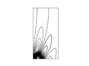
  $\boldsymbol {v}_G$. Figure 2 shows these functions for an exemplary Ta. All three functions are symmetric about $z=1/2$; $s_s$ and $s_\varphi$ are maximal at $z=0$ while $s_z=0$ there. At the ${\textit {Ta}}$ of figure 2 and all other inspected ${\textit {Ta}}$, the function $\sqrt {s_s^2 + s_\varphi ^2 + s_z^2}$ still is maximal at $z=0$, so that
 \begin{equation} \frac{1}{{\textit{Ra}}} \| \boldsymbol{v} \|_\infty \leqslant s_s(0)+s_\varphi(0), \end{equation}
where  $\| \boldsymbol {v} \|_\infty$ denotes the supremum of $| \boldsymbol {v}|$ taken over the entire volume. In a next step, $s_s(0)$ and $s_\varphi (0)$ are computed for different Ta. The result is shown in figure 3. At large ${\textit {Ta}}$, $s_s(0) \ll s_\varphi (0)$ because $s_s(0)$ asymptotes to $s_s(0)=9 {\textit {Ta}}^{-1/2}$, whereas $s_\varphi (0)$ approaches $s_\varphi (0) = 1.23 {\textit {Ta}}^{-1/3}$. The exponents are familiar from vertical shear layers in rotating flows (Stewartson Reference Stewartson1957). As seen in the figure, these power laws are approached from below so that they can be used as upper bounds. We conclude that
 \begin{equation} \| \boldsymbol{v} \|_\infty \leqslant 1.23 {\textit{Ra}} {\textit{Ta}}^{{-}1/3}. \end{equation}
Figure 2. Values of  $s_s$ (dot dashed), $s_\varphi$ (dotted) and $s_z$ (dashed) as functions of height $z$ for ${\textit {Ta}}=10^6$. The solid line shows $\sqrt {s_s^2 + s_\varphi ^2 + s_z^2}$.

Figure 3. Values of  $s_\varphi (0)$ (circles) and $s_s(0)$ (squares) together with the functions $1.23 {\textit {Ta}}^{-1/3}$ (solid) and $9 {\textit {Ta}}^{-1/2}$ (dashed).
This bound is entirely obtained from numerical evaluation of the Green's function and is not supported by an analytical calculation in an asymptotic limit as the other results in this paper. An analytical treatment of (3.52) is arduous because of the absolute values in the integrand which are essential even at  $z=0$. This is due to an interesting point about the structure of $\boldsymbol {v}_G$ shown for an example in figure 4. The source term in (3.42) corresponds to an upward pointing force. The upwelling driven by this force, in conjunction with the boundaries, generates a converging flow below the source and a diverging flow above it. The Coriolis force then gives rise to a cyclonic circulation below the source and an anticyclonic swirl above it. These are indeed the main features observed in figure 4. However, there is also an anticyclonic ring that develops at some distance from the source near $z=0$. This anticyclonic ring weakens as the source moves away from the boundary and is clearly the result of the interaction with the boundary. This ring also causes a change of sign in $v_{G\varphi }$ on $z=0$ as a function of $s$ and makes the absolute value in (3.52) indispensable. Figure 4 plots the product $s v_{G,\varphi }$ rather than $v_{G,\varphi }$ alone to clearly display the change of sign.

Figure 4. Contour plot of the circulation  $s v_{G,\varphi }$ (a) and the streamlines of the meridional part of $\boldsymbol {v}_G$, $(v_{G,s},0,v_{G,z})$ (b) in a vertical plane for a source located at height $z=0.1$ on the axis $s=0$ for ${\textit {Ta}}=10^6$. Dashed contour lines indicate anticyclonic circulation.
4. General Prandtl number
4.1. The additional constraint
The previous section derived bounds on the heat advection and the kinetic energy of the field  $\boldsymbol {v}$ defined by (2.12). These are simultaneously bounds on Nusselt number and total kinetic energy for convection at infinite ${\textit {Pr}}$. At finite ${\textit {Pr}}$, the velocity field is $\boldsymbol {v} + \boldsymbol {u}$. A bound on $\boldsymbol {u}$ is provided by the time average of (2.14)
 \begin{equation} \langle \overline{ |\boldsymbol{\nabla}\boldsymbol{u}|^2 } \rangle ={-}\frac{1}{{\textit{Pr}}} \langle \overline{ \boldsymbol{u} \boldsymbol{\cdot} \partial_t \boldsymbol{v} } \rangle +\frac{1}{{\textit{Pr}}} \langle \overline{\boldsymbol{v} \boldsymbol{\cdot} \left[ (\boldsymbol{u} + \boldsymbol{v}) \boldsymbol{\cdot} \boldsymbol{\nabla}\right] \boldsymbol{u}} \rangle ,\end{equation}
where  $\langle \boldsymbol {u} \boldsymbol {\cdot } [ (\boldsymbol {u} + \boldsymbol {v}) \boldsymbol {\cdot } \boldsymbol {\nabla }] \boldsymbol {v} \rangle =-\langle \boldsymbol {v} \boldsymbol {\cdot } [ (\boldsymbol {u} + \boldsymbol {v}) \boldsymbol {\cdot } \boldsymbol {\nabla }] \boldsymbol {u} \rangle$ was used. One readily bounds the last term from
 \begin{align} |\langle \overline{\boldsymbol{v} \boldsymbol{\cdot} \left[ (\boldsymbol{u} + \boldsymbol{v}) \boldsymbol{\cdot} \boldsymbol{\nabla}\right] \boldsymbol{u}} \rangle| & \leqslant \left\langle \overline{ \sqrt{\sum_{ij} v_i^2(u_j+v_j)^2} \sqrt{\sum_{ij} (\partial_j u_i)^2} } \right\rangle\nonumber\\ & \leqslant \| \boldsymbol{v} \|_\infty \left\langle \overline{ \sqrt{|\boldsymbol{u} + \boldsymbol{v}|^2} \sqrt{|\boldsymbol{\nabla}\boldsymbol{u}|^2} }\right\rangle\nonumber\\ & \leqslant \| \boldsymbol{v} \|_\infty \sqrt{\langle \overline{|\boldsymbol{u} + \boldsymbol{v}|^2} \rangle } \sqrt{\langle \overline{|\boldsymbol{\nabla}\boldsymbol{u}|^2} \rangle }. \end{align}
 The term with the time derivative on the other hand gives rise to another variational problem;  $\partial _t \boldsymbol {v}$ has a decomposition in poloidal and toroidal scalars $\tilde {\phi }$ and $\tilde {\psi }$ with $\partial _t \boldsymbol {v} = \boldsymbol {\nabla }\times \boldsymbol {\nabla }\times \tilde {\phi } \hat {\boldsymbol {z}} + \boldsymbol {\nabla }\times \tilde {\psi } \hat {\boldsymbol {z}}$, $\tilde {\phi } = \partial _t \phi$, $\tilde {\psi } = \partial _t \psi$ and $\phi$ and $\psi$ are the scalars for the decomposition of $\boldsymbol {v}$ itself; $\tilde {\phi }$ and $\tilde {\psi }$ obey the same boundary conditions as $\phi$ and $\psi$. The relation
 \begin{equation} \langle \boldsymbol{u} \boldsymbol{\cdot} \partial_t \boldsymbol{v} \rangle =\langle (\boldsymbol{\nabla}\times \boldsymbol{u}) \boldsymbol{\cdot} (\boldsymbol{\nabla}\times \tilde{\phi} \hat{\boldsymbol{z}} + \tilde{\psi} \hat{\boldsymbol{z}} ) \rangle, \end{equation}
holds if  $\boldsymbol {v}$ obeys no-penetration boundary conditions. The transformation
 \begin{align} \int\boldsymbol{u} \boldsymbol{\cdot} (\boldsymbol{\nabla}\times \boldsymbol{\nabla}\times \tilde{\phi} \hat{\boldsymbol{z}} + \boldsymbol{\nabla}\times \tilde{\psi} \hat{\boldsymbol{z}}) \,\mathrm{d}V &= \int (\boldsymbol{\nabla}\times \boldsymbol{u}) \boldsymbol{\cdot} (\boldsymbol{\nabla}\times \tilde{\phi} \hat{\boldsymbol{z}} + \tilde{\psi} \hat{\boldsymbol{z}} ) \,\mathrm{d}V\nonumber\\ &\quad + \oint \hat{\boldsymbol{n}} \boldsymbol{\cdot} \left[ \boldsymbol{u} \times \begin{pmatrix} \partial_y \tilde{\phi} \\ -\partial_x \tilde{\phi} \\ 0 \end{pmatrix} \right] \mathrm{d}A \!+\! \oint \hat{\boldsymbol{n}} \boldsymbol{\cdot} \left[ \boldsymbol{u} \!\times\! \tilde{\psi} \hat{\boldsymbol{z}} \right] \mathrm{d}A, \end{align}
is independent of boundary conditions;  $\hat {\boldsymbol {n}}$ is the outward pointing normal vector to the surface bounding a periodicity volume. The contribution to the boundary integrals from the vertical faces of the periodicity volume cancel because of periodicity; $\hat {\boldsymbol {n}} \propto \hat {\boldsymbol {z}}$ on the remaining faces. The second boundary integral is zero for $\hat {\boldsymbol {n}} \propto \hat {\boldsymbol {z}}$ independently of the behaviour of $\tilde {\psi }$, and the first integral is zero because $\tilde {\phi }=0$ on $z=0$ and $z=1$.
The Schwarz inequality
 \begin{equation} |\langle \overline{\boldsymbol{u} \boldsymbol{\cdot} \partial_t \boldsymbol{v} } \rangle| \leqslant \sqrt{\langle \overline{|\boldsymbol{\nabla}\times \boldsymbol{u}|^2} \rangle } \sqrt{\langle \overline{|\boldsymbol{\nabla}\times \tilde{\phi} \hat{\boldsymbol{z}}|^2} \rangle +\langle \overline{ \tilde{\psi}^2} \rangle} \end{equation}
motivates us to seek bounds for  $\langle |\boldsymbol {\nabla }\times \tilde {\phi } \hat {\boldsymbol {z}}|^2 \rangle$ and $\langle \tilde {\psi }^2 \rangle$. The time variation of $\phi$ and $\psi$ derives from the time dependence of $\theta$. Let us rewrite (2.5) as ${\textit {Ra}} \partial _t \theta = \boldsymbol {\nabla }\boldsymbol {\cdot } \boldsymbol {q}$ with $\boldsymbol {q} = {\textit {Ra}} \boldsymbol {\nabla }\theta -{\textit {Ra}} (\boldsymbol {u} + \boldsymbol {v}) (T-\frac {1}{2})$ and take time derivatives of (3.2) and (3.3) to find
 \begin{gather} \nabla^2 \nabla^2 \varDelta_2 \tilde{\phi} -\sqrt{{\textit{Ta}}} \partial_z \varDelta_2 \tilde{\psi} = \varDelta_2 \boldsymbol{\nabla}\boldsymbol{\cdot} \boldsymbol{q} , \end{gather}
 \begin{gather}\nabla^2 \varDelta_2 \tilde{\psi} + \sqrt{{\textit{Ta}}} \partial_z \varDelta_2 \tilde{\phi} = 0 . \end{gather}
Before starting the next variational problem, we first note that the preceding equations may alternatively be written as a direct time derivative of (2.12) as
 \begin{equation} 0 ={-} \boldsymbol{\nabla}\tilde p_\infty + \nabla^2 \tilde{\boldsymbol{v}} + \hat{\boldsymbol{z}} (\boldsymbol{\nabla}\boldsymbol{\cdot} \boldsymbol{q} ) -\sqrt{{\textit{Ta}}} \hat{\boldsymbol{z}} \times \tilde{\boldsymbol{v}}, \end{equation}
with  $\tilde p_\infty = \partial _t p_\infty$ and $\tilde {\boldsymbol {v}} = \partial _t \boldsymbol {v}$. Taking the scalar product of this equation with $\tilde {\boldsymbol {v}}$ and averaging over all space leads to
 \begin{equation} \langle |\boldsymbol{\nabla}\tilde{\boldsymbol{v}}|^2 \rangle = \langle \tilde{v}_z (\boldsymbol{\nabla}\boldsymbol{\cdot}\boldsymbol{q} ) \rangle ={-} \langle (\boldsymbol{\nabla}\tilde{v}_z) \boldsymbol{\cdot} \boldsymbol{q} \rangle \leqslant \sqrt{\langle |\boldsymbol{\nabla}\tilde{v}_z|^2 \rangle} \sqrt{\langle |\boldsymbol{q}|^2 \rangle} \leqslant \sqrt{\langle |\boldsymbol{\nabla}\tilde{\boldsymbol{v}}|^2 \rangle} \sqrt{\langle |\boldsymbol{q}|^2 \rangle}, \end{equation}
and hence  $\langle |\boldsymbol {\nabla }\tilde {\boldsymbol {v}}|^2 \rangle \leqslant \langle |\boldsymbol {q}|^2 \rangle$. Both $\langle |\boldsymbol {\nabla }\times \tilde {\phi } \hat {\boldsymbol {z}}|^2 \rangle$ and $\langle \tilde {\psi }^2 \rangle$ are bounded in terms of $\langle |\boldsymbol {\nabla }\tilde {\boldsymbol {v}}|^2 \rangle$ because of the Poincaré inequality, which means that both quantities are smaller than some finite factor multiplied by $\langle |\boldsymbol {q}|^2 \rangle$. The existence of such finite factors being established, we now proceed to determine ${\textit {Ta}}$ dependent values for these factors from a variational problem.
The source term  $\boldsymbol {q}$ obeys $\boldsymbol {\nabla }\boldsymbol {\cdot } {\boldsymbol {q}} =0$ at $z=0$ and $z=1$, which from (4.6) implies $\partial _z^4 \tilde {\phi } =0$ on those boundaries. Taking the second derivative of (2.5) also leads to $\partial _z^2 \boldsymbol {\nabla }\boldsymbol {\cdot } {\boldsymbol {q}}=0$, so that $\boldsymbol {\nabla }\boldsymbol {\cdot } {\boldsymbol {q}}$ obeys the same boundary conditions as $\theta$ and we can set up a variational problem similar to those of the previous sections for maximizing an objective $Z$ subject to (4.6), (4.7) and $\langle |{\boldsymbol {q}}|^2 \rangle$ fixed to any arbitrary value. This leads to a Lagrangian analogous to (3.5):
 \begin{align} {{\mathcal{L}}} &= \int \left\{ Z - \mu_1(\boldsymbol{r}) \left[ \nabla^2 \nabla^2 \varDelta_2 \tilde{\phi} -\sqrt{{\textit{Ta}}} \partial_z \varDelta_2 \tilde{\psi} -\varDelta_2 \boldsymbol{\nabla}\boldsymbol{\cdot} {\boldsymbol{q}} \right]\right.\nonumber\\ &\quad \left.- \mu_2(\boldsymbol{r}) \left[ \nabla^2 \varDelta_2 \tilde{\psi} + \sqrt{{\textit{Ta}}} \partial_z \varDelta_2 \tilde{\phi} \right]- \lambda |{\boldsymbol{q}}|^2\right\} \mathrm{d}V . \end{align}
The Euler–Lagrange equations again lead to an eigenvalue problem for  $\lambda$ and the largest eigenvalue $\lambda _{max}$ provides us with the inequality $\langle Z \rangle \leqslant \lambda _{max} \langle |{\boldsymbol {q}}|^2 \rangle$.
To simplify the algebra, it is convenient to choose  $Z=a |\boldsymbol {\nabla }\times \tilde {\phi } \hat {\boldsymbol {z}}|^2 + b \tilde {\psi }^2$ in which we can set the coefficients $a$ and $b$ alternatively to 0 and 1. The variations with respect to ${\boldsymbol {q}}$, $\tilde {\psi }$, and $\tilde {\phi }$, respectively yield,
 \begin{gather} \boldsymbol{\nabla}\varDelta_2 \mu_1 + 2 \lambda {\boldsymbol{q}} = 0 , \end{gather}
 \begin{gather}2 b \tilde{\psi} - \sqrt{{\textit{Ta}}} \partial_z \varDelta_2 \mu_1 - \nabla^2 \varDelta_2 \mu_2 = 0 , \end{gather}
 \begin{gather}-2 a \varDelta_2 \tilde{\phi} - \nabla^2 \nabla^2 \varDelta_2 \mu_1 + \sqrt{{\textit{Ta}}} \partial_z \varDelta_2 \mu_2 = 0, \end{gather}
from which one deduces
 \begin{equation} \lambda {\mathcal{D}} {\mathcal{D}} \varDelta_2 \tilde{\phi} = a \nabla^2 \nabla^2 \nabla^2 \varDelta_2 \varDelta_2 \tilde{\phi} +b {\textit{Ta}} \partial_z^2 \nabla^2 \varDelta_2 \tilde{\phi}. \end{equation}
Insertion of the sinusoidal eigenfunction and the substitutions  $k^2=k_x^2+k_y^2=n^2 {\rm \pi}^2 \xi$ and $\tau = {{\textit {Ta}}}/{n^4 {\rm \pi}^4}$ lead to
 \begin{equation} \lambda = \frac{1}{n^4 {\rm \pi}^4} \frac{(1+\xi) [b \tau + a\xi(1+\xi)^2]}{[(1+\xi)^3+\tau]^2}. \end{equation}
Let us first select  $a=0$ and $b=1$. The necessary condition for the maximizing $\xi$ becomes
 \begin{equation} \tau [\tau - 5(1+\xi)^3] = 0, \end{equation}
which is solved by  $\xi =(\tau /5)^{1/3}-1$ without any asymptotic approximation and from which we can deduce
 \begin{equation} \langle \tilde{\psi}^2 \rangle \leqslant \frac{5^{5/3}}{36 {\rm \pi}^{4/3}} {\textit{Ta}}^{{-}2/3} \langle |{\boldsymbol{q}}|^2 \rangle. \end{equation}
 In the opposite case  $a=1$, $b=0$, the necessary condition for the maximizing $\xi$ becomes
 \begin{equation} (1+\xi)^3 (1-2\xi) + \tau (1+4\xi) = 0, \end{equation}
which requires for  $\xi \gg 1$ that $\xi ^3 = 2\tau$. The maximal eigenvalue $\lambda _4$ is realized for $n=1$ and is asymptotically
 \begin{equation} \lambda_4 = \frac{2}{9} \left(\frac{2}{{\rm \pi}^4} \right)^{1/3} {\textit{Ta}}^{{-}2/3}, \end{equation}
which also constitutes an upper bound for the largest root of (4.18) for reasonably large  ${\textit {Ta}}$ (see figure 1d) so that we arrive at
 \begin{equation} \langle |\boldsymbol{\nabla}\times \tilde{\phi} \hat{\boldsymbol{z}}|^2 \rangle + \langle \tilde{\psi}^2 \rangle \leqslant \left( \frac{5^{5/3}}{36}+\frac{2^{4/3}}{9} \right) \frac{1}{{\rm \pi}^{4/3}} {\textit{Ta}}^{{-}2/3} \langle |{\boldsymbol{q}}|^2 \rangle \lesssim 0.15 {\textit{Ta}}^{{-}2/3} \langle |{\boldsymbol{q}}|^2 \rangle. \end{equation}
With the maximum principle,  $\langle |(\boldsymbol {u} + \boldsymbol {v})(T-\frac {1}{2})|^2 \rangle \leqslant \frac {1}{4} \langle |(\boldsymbol {u} + \boldsymbol {v})|^2 \rangle$, and the triangle inequality in the form $\langle |(\boldsymbol {a} + \boldsymbol {b})|^2 \rangle \leqslant 2 \langle |\boldsymbol {a}|^2 \rangle + 2 \langle |\boldsymbol {b}|^2 \rangle$, it follows from the definition of ${\boldsymbol {q}}$ that
 \begin{equation} \frac{1}{{\textit{Ra}}^2} \langle |{\boldsymbol{q}}|^2 \rangle \leqslant 2 \langle |\boldsymbol{\nabla}\theta|^2 \rangle + \frac{1}{2} \langle |(\boldsymbol{u} + \boldsymbol{v})|^2 \rangle, \end{equation}
and we finally arrive at
 \begin{equation} |\langle \overline{\boldsymbol{u} \boldsymbol{\cdot} \partial_t \boldsymbol{v} } \rangle| \leqslant \sqrt{\langle \overline{|\boldsymbol{\nabla}\boldsymbol{u}|^2} \rangle } \sqrt{0.15} {\textit{Ra}} {\textit{Ta}}^{{-}1/3} \left( \sqrt{2 \langle \overline{|\boldsymbol{\nabla}\theta|^2} \rangle} + \sqrt{\frac{1}{2} \langle \overline{|(\boldsymbol{u} + \boldsymbol{v})|^2} \rangle} \right), \end{equation}
where  $\langle \overline {|\boldsymbol {\nabla }\times \boldsymbol {u}|^2} \rangle = \langle \overline {|\boldsymbol {\nabla }\boldsymbol {u}|^2} \rangle$ was used.
We can now return to (4.1) and insert (4.2), (3.54), (4.22) to find
 \begin{equation} \left.\begin{gathered} \sqrt{\langle \overline{|\boldsymbol{\nabla}\boldsymbol{u}|^2} \rangle } \leqslant c_1 \sqrt{\langle \overline{|\boldsymbol{\nabla}\theta|^2} \rangle} + c_2 \sqrt{\langle \overline{|(\boldsymbol{u} + \boldsymbol{v})|^2} \rangle} ,\\ c_1 = \sqrt{0.3} \frac{1}{{\textit{Pr}}} {\textit{Ra}} {\textit{Ta}}^{{-}1/3} , \\ c_2 = (\sqrt{0.075}+1.23) \frac{1}{{\textit{Pr}}} {\textit{Ra}} {\textit{Ta}}^{{-}1/3} . \end{gathered}\right\} \end{equation}
With  $c_0=\max \{1,{L}/{2} \}$ and the Poincaré inequality $\sqrt {\langle \overline {|(\boldsymbol {u} \!+\! \boldsymbol {v})|^2} \rangle } \!\leqslant\! ({1}/{{\rm \pi} } )c_0 \sqrt {\langle \overline {|\boldsymbol {\nabla }(\boldsymbol {u} \!+\! \boldsymbol {v})|^2} \rangle }$ from (2.15), and (2.10) and (2.11), this can be rewritten as
 \begin{equation} \sqrt{\langle \overline{|\boldsymbol{\nabla}\boldsymbol{u}|^2} \rangle } \leqslant \left(c_1 + \frac{c_2}{\rm \pi} c_0 {\textit{Ra}}^{1/2} \right)\sqrt{\langle \overline{|\boldsymbol{\nabla}\theta|^2} \rangle}. \end{equation}
4.2. Bound on the Nusselt number
Equations (2.11) and (2.8) lead to
 \begin{equation} \langle \overline{|\boldsymbol{\nabla}\theta|^2} \rangle = \langle \overline{v_z \theta } \rangle + \langle \overline{u_z \theta } \rangle \leqslant \langle \overline{v_z \theta } \rangle +\sqrt{\frac{7}{12}} \sqrt{\langle \overline{u_z^2} \rangle }, \end{equation}
in which we may insert the Poincaré inequality  $\sqrt {\langle \overline {u_z^2} \rangle } \leqslant {1}/{{\rm \pi} } \sqrt {\langle \overline {(\partial _z u_z)^2} \rangle }$ and $\langle (\partial _z u_z)^2 \rangle \leqslant \frac {1}{4} \langle |\boldsymbol {\nabla }\boldsymbol {u}|^2 \rangle$ (Doering & Constantin Reference Doering and Constantin1996) together with (4.24) and (3.17) to find
 \begin{equation} \langle \overline{|\boldsymbol{\nabla}\theta|^2} \rangle - \frac{1}{2{\rm \pi}} \sqrt{\frac{7}{12}} \left(c_1 + \frac{c_2}{\rm \pi} c_0 {\textit{Ra}}^{1/2} \right)\sqrt{\langle \overline{|\boldsymbol{\nabla}\theta|^2} \rangle} \leqslant \frac{7}{36} \left(\frac{4}{{\rm \pi}^2} \right)^{1/3} {\textit{Ra}} {\textit{Ta}}^{{-}1/3}. \end{equation}
We finally deduce
 \begin{equation} \left.\begin{gathered} {\textit{Nu}}-1 = \langle \overline{|\boldsymbol{\nabla}\theta|^2} \rangle \leqslant \frac{7}{36} \left(\frac{4}{{\rm \pi}^2} \right)^{1/3} {\textit{Ra}} {\textit{Ta}}^{{-}1/3} (\sqrt{1+A^2}+A)^2 ,\\ A = [0.088+0.077 c_0 {\textit{Ra}}^{1/2}] {\textit{Pr}}^{{-}1} {\textit{Ra}}^{1/2} {\textit{Ta}}^{{-}1/6}. \end{gathered}\right\}\end{equation}
It is found that  $A \rightarrow 0$ for ${\textit {Pr}} \rightarrow \infty$ and (3.17) is recovered as a special case of (4.27).
4.3. Bounds on the velocity field
With the triangle and Poincaré inequalities,
 \begin{equation} \sqrt{\langle \overline{|(\boldsymbol{u} + \boldsymbol{v})|^2} \rangle} \leqslant \sqrt{\langle \overline{|\boldsymbol{v}|^2} \rangle} + \frac{1}{\rm \pi} c_0 \sqrt{\langle \overline{|\boldsymbol{\nabla}\boldsymbol{u}|^2} \rangle } ,\end{equation}
which becomes with (4.23), (2.11), (2.8) and (3.31)
 \begin{align} &\sqrt{\langle \overline{|(\boldsymbol{u} + \boldsymbol{v})|^2} \rangle} -\frac{1}{\rm \pi} c_0 \left(c_1 + \frac{c_2}{\rm \pi} c_0 {\textit{Ra}}^{1/2} \right) \left( \frac{7}{12} \right)^{1/4} \langle \overline{|(\boldsymbol{u} + \boldsymbol{v})|^2} \rangle^{1/4} \nonumber\\ &\quad \leqslant \sqrt{\frac{7}{36}} \left( \frac{4}{\rm \pi} \right)^{1/6} \frac{1}{\sqrt{\rm \pi}} {\textit{Ra}} {\textit{Ta}}^{{-}1/3}, \end{align}
from which we can conclude that
 \begin{equation} \left.\begin{gathered} \sqrt{\langle \overline{|(\boldsymbol{u} + \boldsymbol{v})|^2} \rangle} \leqslant \frac{\sqrt{7}}{6} 4^{1/6} {\rm \pi}^{{-}2/3} {\textit{Ra}} {\textit{Ta}}^{{-}1/3} (\sqrt{1+B^2}+B)^2 ,\\ B = c_0 [0.15+0.13 c_0 {\textit{Ra}}^{1/2}] {\textit{Pr}}^{{-}1} {\textit{Ra}}^{1/2} {\textit{Ta}}^{{-}1/6}. \end{gathered}\right\}\end{equation}
Once again, this formula includes the result (3.31) for infinite Prandtl number convection because  $B \rightarrow 0$ for ${\textit {Pr}} \rightarrow \infty$.
It is also possible to generalize (3.35). Start again from (4.28) and substitute (4.24) and (3.35) to obtain
 \begin{equation} \sqrt{\langle \overline{|(\boldsymbol{u} + \boldsymbol{v})|^2} \rangle} \leqslant \left\{ 1+ c_0 [0.55 + 0.48 c_0 {\textit{Ra}}^{1/2}] \frac{{\textit{Ta}}^{1/6}}{{\textit{Pr}}} \right\} \frac{{\textit{Ra}} {\textit{Ta}}^{{-}1/2}}{\rm \pi} \sqrt{ \langle \overline{|\boldsymbol{\nabla}\theta|^2} \rangle }. \end{equation}
5. Discussion
The main results of this paper are the bounds for  ${\textit {Nu}}$ and the kinetic energy at infinite ${\textit {Pr}}$ in (3.17), (3.31), (3.35) together with the pointwise bound on the magnitude of the velocity at infinite ${\textit {Pr}}$ in (3.54). The first three bounds are extended to finite ${\textit {Pr}}$ in (4.27), (4.30), (4.31).
The bound for  ${\textit {Nu}}$ in (4.27) is valid as long as ${\textit {Ta}} > 130$, which was necessary for the estimation of the largest root of the polynomial in (3.15). This bound reduces to a simpler expression for infinite Prandtl number already given in (3.17). The critical Rayleigh number for the onset of convection, ${\textit {Ra}}_{crit}$, is proportional to ${\textit {Ta}}^{2/3}$ (Chandrasekhar Reference Chandrasekhar1961). Ignoring numerical prefactors, the bound (3.17) may be rewritten as ${\textit {Nu}}-1 \lesssim {\textit {Ra}}^{1/2} ({\textit {Ra}}/{\textit {Ra}}_{crit})^{1/2}$. This may be compared with the bound derived in Constantin et al. (Reference Constantin, Hallstrom and Putkaradze1999) which is apart from a prefactor ${\textit {Nu}}-1 \lesssim {\textit {Ra}}^{1/2} ({\textit {Ra}}/{\textit {Ra}}_{crit})^{3/2}$. Both of these bounds are inferior to the uniformly valid ${\textit {Nu}}-1 \lesssim {\textit {Ra}}^{1/2}$ as soon as ${\textit {Ra}} > {\textit {Ra}}_{crit}$. For ${\textit {Ra}} < {\textit {Ra}}_{crit}$, the result in Constantin et al. (Reference Constantin, Hallstrom and Putkaradze1999) is the sharper bound, which is not surprising since the bound (3.17) was derived without explicit reference to the temperature equation. However, the bound (3.17) has the merit to be generalizable to finite ${\textit {Pr}}$ in (4.27).
The bounds for general  ${\textit {Pr}}$ and free-slip boundaries depend on the periodicity length and diverge if this length tends to infinity. However, if one wants to model a geometry similar to a deep spherical shell, such as the Earth's outer core, the vertical extent is of the same order of magnitude as the lateral periodicity length and the dependence on the periodicity length is not a major concern.
As soon as a bound on  ${\textit {Nu}}$ is available, the Poincaré inequality yields a bound at least on the poloidal kinetic energy through a Poincaré inequality. Previous numerical optimization (Tilgner Reference Tilgner2017a) obtained a better prefactor but not better exponents of the control parameters than obtained from the Poincaré inequality, neither at infinite nor at finite ${\textit {Pr}}$. The bound derived in the present paper is a novelty in this respect. Straightforward application of the Poincaré inequality to either (3.17) or the bound from Constantin et al. (Reference Constantin, Hallstrom and Putkaradze1999) leads to $\langle \overline {|\boldsymbol {v}|^2} \rangle \lesssim {\textit {Ra}}^2 {\textit {Ta}}^{-1/3}$ or $\langle \overline {|\boldsymbol {v}|^2} \rangle \lesssim {\textit {Ra}}^3 / {\textit {Ta}}$, both of which are inferior to (3.31) for ${\textit {Ra}} > {\textit {Ra}}_{crit}$. In the same manner, inequality (3.35), which is the reduction of (4.31) to infinite ${\textit {Pr}}$, says that $\langle \overline {|\boldsymbol {v}|^2} \rangle \lesssim ({\textit {Nu}}-1) {\textit {Ra}}^2 / {\textit {Ta}}$, which is better than the result from the Poincaré inequality for ${\textit {Ra}} < {\textit {Ta}}$.
However, the bounds on neither  ${\textit {Nu}}$ nor $\langle \overline {|(\boldsymbol {u} + \boldsymbol {v})|^2} \rangle$ reproduce the fact observed in both experiments and simulations that ${\textit {Nu}}-1$ and $\langle \overline {|(\boldsymbol {u} + \boldsymbol {v})|^2} \rangle$ approach zero at ${\textit {Ra}} = {\textit {Ra}}_{crit}$. The exponents in both bounds can be obtained by simply inserting (3.54) into $\langle v_z \theta \rangle \leqslant \| \boldsymbol {v} \|_\infty$ and $\langle |\boldsymbol {v}|^2 \rangle \leqslant \| \boldsymbol {v} \|_\infty ^2$.
The complexity of the calculation is reduced in this paper by solving two problems sequentially. In a first step, the constraints imposed by the momentum equation and the maximum principle are used at infinite  ${\textit {Pr}}$. No use of the temperature equation is made. It is then simple to obtain in a second step rotation dependent bounds at arbitrary ${\textit {Pr}}$ by including the constraint (4.24). A more comprehensive approach would be to solve an optimization problem which simultaneously includes the momentum equation, the temperature equation, and the constraint (4.24). This set of constraints guarantees tighter bounds for ${\textit {Nu}}$ at infinite ${\textit {Pr}}$ and presumably also improves the bounds at general ${\textit {Pr}}$. However, this more involved problem will likely need a numerical optimization for its solution and is left for future work.
Inequalities like (3.35) or (4.31) may look like weak statements from the mathematical point of view because they relate  ${\textit {Nu}}$ to both the control parameters and the kinetic energy, which is itself a result of the dynamics. However, these relations are more immediately applicable to geophysical and astrophysical situations than the other bounds, because the Rayleigh number is frequently impossible to determine from observations. To motivate the derivation of relations of this type and to keep the discussion simple, let us look at how the form for infinite Prandtl number may become useful and use dimensional variables. If the convecting fluid has viscosity $\nu$, thermal diffusivity $\kappa$, density $\rho$, heat capacity $c_p$ and expansion coefficient $\alpha$, its velocity $\boldsymbol {V}$ must be related to the non-dimensional velocity $\boldsymbol {v}$ by $\boldsymbol {V} = \boldsymbol {v} \kappa /d$ in order to obtain (2.4), where $d$ is the depth of the layer. If the heat flux through the layer is $Q$ and the temperature difference across the layer is $\Delta T$, the rotation rate of the frame of reference is $\varOmega$ and the gravitational acceleration is $g$, the control parameters in (2.4) are given by
 \begin{equation} {\textit{Ra}} = \frac{g \alpha \Delta T d^3}{\kappa \nu} , \quad {\textit{Pr}} = \frac{\nu}{\kappa} , \quad {\textit{Ta}}=\frac{4 \varOmega^2 d^4}{\nu^2}, \end{equation}
and
 \begin{equation} {\textit{Nu}} = \frac{Q d}{\kappa \rho c_p \Delta T}. \end{equation}
Assuming  ${\textit {Nu}}-1 \approx {\textit {Nu}}$, (3.35) can be rearranged into
 \begin{equation} \Delta T \geqslant \left( \frac{2 {\rm \pi}\varOmega}{g \alpha} \right)^2 \frac{\kappa \rho c_p}{Q d} \langle \overline{|\boldsymbol{V}|^2} \rangle. \end{equation}
Let us take convection in the Earth's core as an example and pretend that the above relation is applicable to a spherical shell in the presence of a magnetic field. We ignore these features for now because the relevant point to be made about this relation does not concern specific values of prefactors or exponents, but depends on which quantities are well known and which are not. The rotation rate, the depth of the layer, and the gravitational acceleration are well known, and there are reasonable estimates of the material properties. Temporal variations of the geomagnetic field provide us with some information about  $\langle \overline {|\boldsymbol {V}|^2} \rangle$, and the heat flux through the Earth's surface constrains $Q$. On the other hand, $\Delta T$ is essentially unknown. A relation of the form of (4.31) thus allows us to put a constraint on a quantity impossible to determine otherwise.
Another deduction from (4.31) is a bound on a characteristic length  $\ell$ of the flow defined as $\ell ^2 = \langle \overline {|(\boldsymbol {u} + \boldsymbol {v})|^2} \rangle / \langle \overline {|\boldsymbol {\nabla }(\boldsymbol {u} + \boldsymbol {v})|^2} \rangle$. It follows from (4.31) and (2.10), together with the assumption ${\textit {Ra}}^{1/2} \gg 1$, that
 \begin{equation} \ell \leqslant \frac{1}{\rm \pi} \left( \frac{{\textit{Ra}}}{{\textit{Ta}}} \right)^{1/2} \left( 1 + 0.48 c_0 \frac{{\textit{Ra}}^{1/2}{\textit{Ta}}^{1/6}}{{\textit{Pr}}} \right). \end{equation}
This inequality puts a formal limit on the structure of a condensate or a large eddy as observed in numerical simulations (Guervilly, Hughes & Jones Reference Guervilly, Hughes and Jones2014).
The simplification brought about by the infinite Prandtl number is that the time derivative and advection terms disappear from the momentum equation (2.4). At large  ${\textit {Pr}}$, these terms are small compared with the viscous term. However, the two terms can also be negligible in comparison with the Coriolis term. Many results in classical geophysical fluid dynamics are based on an approach in which one postulates that the advection term and possibly the time derivative term are small, one solves the thus linearized momentum equation, and one finds good agreement for many large scale phenomena (Vallis Reference Vallis2017). This is not a widespread approach in simulations of convection (but see Calkins, Julien & Tobias Reference Calkins, Julien and Tobias2017), but the inertial terms are found to be negligible with hindsight in some simulations. An example are the simulations in Schmitz & Tilgner (Reference Schmitz and Tilgner2009) (and analogous results for no-slip boundary conditions in Schmitz & Tilgner Reference Schmitz and Tilgner2010). It was found in these simulations that the flows are dominated by the Coriolis force if $\langle \overline {|\boldsymbol {v}|^2} \rangle {\textit {Ta}}^{-1/2} < 1$, in which case the flow is organized into columnar structures, similar to those visualized in Stellmach & Hansen (Reference Stellmach and Hansen2004), which vary slowly in time and whose Rossby number is small. The time derivative and advection terms in these flows are small even though the Prandtl number is not large. These flows are good candidates to be modelled by the momentum equation with these terms dropped. It therefore makes sense to compare the numerical results of Schmitz & Tilgner (Reference Schmitz and Tilgner2009) not only with the bound (4.31), but also with the bound (3.35) in the form $\langle \overline {|\boldsymbol {v}|^2} \rangle {\textit {Ta}} \leqslant {\textit {Ra}}^2 ({\textit {Nu}}-1) / {\rm \pi}^2$ which is done in figure 5. As one can see, the latter bound is within an order of magnitude of the actual results. It remains a challenge for the future to prove ab initio that the inertial terms are negligible at the parameters of this figure. The bound (4.31) lies several orders of magnitude above the numerical data.

Figure 5. Value of  $\langle \overline {|\boldsymbol {v}|^2}\rangle Ta \, Ra^{-2} (Nu-1)^{-1}$ as a function of $\langle \overline {|\boldsymbol {v}|^2}\rangle Ta^{-1/2}$ for ${\textit {Pr}}=7$ (red symbols) and ${\textit {Pr}}=0.7$ (blue symbols). The symbol shape stands for ${\textit {Ta}}=10^4$ (diamonds), $10^6$ (squares), $10^8$ (triangles) and $10^{10}$ (stars). The dashed horizontal line indicates $1/{\rm \pi} ^2$.
Declaration of interests
The authors report no conflict of interest.


 Open access