


1. Introduction
Flows involving body forces are widely present in nature and engineering practice. Examples include gravity-induced natural convection such as in Rayleigh–Bénard flows, flows in rotating reference system influenced by centrifugal and Coriolis forces, magneto-fluid influenced by electromagnetic force and many others. In the fast-growing lattice Boltzmann method (LBM), correctly incorporating the body force has an added importance as the body force is also used to model inter-particle interactions giving rise to the rich phenomena of multiphase flows (Shan & Chen Reference Shan and Chen1993; He, Shan & Doolen Reference He, Shan and Doolen1998b).
Although the treatment of body force is rather straightforward in both hydrodynamic equations and the Boltzmann equation, it remains a non-trivial and sometimes even controversial topic for the LBM after a substantial amount of effort and literally a dozen proposed schemes (Mohamad & Kuzmin Reference Mohamad and Kuzmin2010; Bawazeer, Baakeem & Mohamad Reference Bawazeer, Baakeem and Mohamad2021). The difficulty can be arguably attributed to the fact that the LBM was developed from beginning as a discrete kinetic model that was tailored a posteriori to exhibit Navier–Stokes–Fourier thermohydrodynamics at the macroscopic level. It lacked a first-principle theory dictating the evolution of the discrete distribution in an external force field. Furthermore, from the perspective of kinetic theory, the configuration-velocity phase space was discretised together, making error analysis complicated.
An early idea was suggested by Shan & Chen (Reference Shan and Chen1993) to shift the equilibrium velocity in the collision term to account for the change of momentum which is the leading-order effect of body force. This approach only imposes a condition on the zeroth and first moments of the discrete distribution function. Although reasonably successful in simple flows, subtle issues arose in applications where detailed modelling of the body-force effect is required. An example is the multiphase fluid where the velocity-shift scheme results in unphysical dependence of the equilibrium densities on the relaxation time (Yu & Fan Reference Yu and Fan2009). Sbragaglia et al. (Reference Sbragaglia, Benzi, Biferale, Chen, Shan and Succi2009) eliminated the inaccuracy in energy equation by also shifting the temperature. Using the method of undetermined coefficients and matching the macroscopic equation out of Chapman–Enskog calculation with the Navier–Stokes equation, Guo, Zheng & Shi (Reference Guo, Zheng and Shi2002) gave a scheme to eliminate the discrete lattice effect caused by spatial–temporal discretisation, which also removed the unphysical dependency on the relaxation time when applied to the multiphase model. This line of approach (Buick & Greated Reference Buick and Greated2000; Ladd & Verberg Reference Ladd and Verberg2001) calls upon a posteriori matching with the hydrodynamic equations and becomes unwieldy when applied to more complicated collision models and higher-order hydrodynamic approximations.
Another strategy is to start from the body-force term of the Boltzmann equation,  $\boldsymbol {g}\boldsymbol {\cdot }\nabla _{\xi } f$. He, Chen & Doolen (Reference He, Chen and Doolen1998a) approximated $f$ by the Maxwell–Boltzmann equilibrium, $f^{(0)}$, and integrated using the trapezoidal rule to advance one time step. An auxiliary variable was introduced to eliminate the implicity. Martys, Shan & Chen (Reference Martys, Shan and Chen1998) pointed out, by examining the Hermite expansion of the body force, that this approximation is exact up to the second moments. By realising that $\nabla _\xi f ^{(0)} = -\nabla _uf^{(0)}$, Kupershtokh (Reference Kupershtokh2004) introduced the exact difference method (EDM) to model the effect of the body force as $f^{(0)}(\rho, \boldsymbol {u}+\boldsymbol {g}{\rm \Delta} t) - f^{(0)}(\rho, \boldsymbol {u})$ which correctly advances a local equilibrium to another one with a shifted velocity. However, effect of the non-equilibrium part of the distribution is ignored all together. In both schemes the spatial–temporal discretisation was carefully handled to achieve second-order accuracy.
Despite that the differences, similarities and accuracies of the existing forcing schemes have been theoretically analysed and numerically examined by a number of authors (Kupershtokh, Medvedev & Karpov Reference Kupershtokh, Medvedev and Karpov2009; Mohamad & Kuzmin Reference Mohamad and Kuzmin2010; Huang, Krafczyk & Lu Reference Huang, Krafczyk and Lu2011; Li, Luo & Li Reference Li, Luo and Li2012; Silva & Semiao Reference Silva and Semiao2012), it remains inconclusive as to which scheme is the most accurate because the results often depend on flow conditions such as compressibility and steadiness. Possible origins of the discrepancies include insufficient expansions of the distribution function, the collision term or the body-force term, all resulting in different error terms in the recovered macroscopic equations. More importantly, as the LBM being extended to thermal compressible flows, the existing works mainly focus on the recovery of the mass and momentum equations, whereas, except for a few works (Sbragaglia et al. Reference Sbragaglia, Benzi, Biferale, Chen, Shan and Succi2009), the body-force effect on the energy equation is rarely discussed.
The LBM can be reformulated using kinetic theory in continuum in two separate steps (Shan & He Reference Shan and He1998; Shan, Yuan & Chen Reference Shan, Yuan and Chen2006). First, the Bhatnagar–Gross–Krook (BGK) model equation is projected into a finite-dimensional Hilbert space spanned by the Hermite polynomials. By choosing a set of discrete velocity coordinates that forms a Gauss–Hermite quadrature rule and evaluating the BGK equation at these velocities, one obtains the dynamic equations for a set of discrete distributions in the configuration space which preserve the moments of the continuum distribution function and, therefore, the hydrodynamics of the BGK equation. Second, the equations for the discrete distribution are further discretised in space and time to yield the lattice Boltzmann equation. With the velocity-space discretisation of the body-force term simply amounted to expanding it in Hermite polynomials, Li, Duan & Shan (Reference Li, Duan and Shan2022) showed that by using second-order time integration on the second-order Hermite expansion of the body-force term, one can recover a priori the force scheme of Guo et al. (Reference Guo, Zheng and Shi2002). Moreover, the methodology is generic so that it can be applied to higher-order moment expansions which give rise to the thermal and non-equilibrium dynamics.
In this paper, we present a systematic discretisation scheme for the body-force term which is second order in space and time, and valid for moments of arbitrary orders. In particular, force terms pertinent to the energy equation are explicitly given, and errors in heat flux caused by insufficient expansion of the force term is also obtained via Chapman–Enskog analysis. Numerical verifications were carried out to show that the third-moment contribution in the force term has a non-negligible effect in flows with strong temperature variation. The remainder of the paper is organised as follows. In § 2, we present the methodology to systematically obtain the force term in LBM. The third-order expansion of the form term is obtained and its necessity in the energy equation is demonstrated in Chapman–Enskog analysis. In § 3, we present numerical verifications and analyses. Some further discussions are given in § 4.
2. Moment expansion of the force term
We first briefly recap the kinetic theoretic formulation of the LBM. We start with the Boltzmann equation with the BGK collision operator,
 \begin{equation} \frac{\partial f}{\partial t} + \boldsymbol{\xi}\boldsymbol{\cdot}\boldsymbol{\nabla} f + \boldsymbol{g}\boldsymbol{\cdot}\nabla_{\xi} f = \varOmega(f) ={-}\frac{1}{\tau}[f-f^{(0)}], \end{equation}
where  $\boldsymbol {x}$ and $\boldsymbol {\xi }$ are the coordinates in physical and velocity spaces, respectively, $t$ is the time, $f(\boldsymbol {x},\boldsymbol {\xi },t)$ is the single-particle distribution function, $\boldsymbol {g}$ is the acceleration of the body force, $\nabla _{\xi }$ is the gradient in velocity space, $\varOmega$ is the collision term, $\tau$ is the relaxation time and $f^{(0)}$ is the Maxwell–Boltzmann equilibrium distribution function:
 \begin{equation} f^{(0)} = \frac{\rho}{(2{\rm \pi} RT)^{D/2}}\exp\left[-\frac{c^2}{2RT}\right], \end{equation}
where  $D$ is the space dimensionality, $R$ is the gas constant, $T$ is the temperature, $\rho$ is the fluid density, $\boldsymbol {c}=\boldsymbol {\xi }-\boldsymbol {u}$, $c^2 = \boldsymbol {c}\boldsymbol {\cdot }\boldsymbol {c}$ and $\boldsymbol {u}$ is the fluid velocity. Following Shan et al. (Reference Shan, Yuan and Chen2006), we use the so-called energy units where $\sqrt {RT_0}$ is the characteristic velocity and $T_0$ is the characteristic temperature. The length and time units, $l_0$ and $t_0$, respectively, satisfy $l_0/t_0 = \sqrt {RT_0}$. After non-dimensionalisation, (2.1) remains the same and (2.2) takes the following form:
 \begin{equation} f^{(0)} = \frac{\rho}{(2{\rm \pi} \theta)^{D/2}}\exp\left[-\frac{c^2}{2\theta}\right], \end{equation}
where  $\theta \equiv T/T_0$ is the dimensionless temperature. Here $\rho$, $\boldsymbol {u}$ and $\theta$, are velocity moments of the distribution function
 \begin{equation} \{\rho, \rho\boldsymbol{u}, D\rho\theta\} = \int f \{1, \boldsymbol{\xi}, c^2\}\, {\rm d} \boldsymbol{\xi}. \end{equation}
The LBM can be formulated as a velocity-space discretisation by first projecting (2.1) into a finite-dimensional functional space spanned by Hermite polynomials and then evaluating at discrete velocities that form a Gauss–Hermite quadrature rule in the velocity space (Grad Reference Grad1949; Shan & He Reference Shan and He1998; Shan et al. Reference Shan, Yuan and Chen2006). The latter requirement ensures that the leading velocity moments are exactly preserved by the discrete distribution function values. A key step in this formulation is to expand all terms in (2.1) into finite Hermite series, assuming  $f$ has the following expansion in the laboratory reference frame:
 \begin{equation} f_N(\boldsymbol{x}, \boldsymbol{\xi}, t) = \omega(\boldsymbol{\xi})\sum_{n=0}^N\frac{1}{n!} {\boldsymbol{a}}^{(n)}(\boldsymbol{x}, t):{\mathcal{H}}^{(n)}(\boldsymbol{\xi}), \end{equation}
where  $N$ is the expansion order, ‘:’ denotes full contraction between two tensors, ${\mathcal {H}}^{(n)}(\boldsymbol {\xi })$ is the $n$th tensorial Hermite polynomial, $\omega (\boldsymbol {\xi })\equiv (2{\rm \pi} )^{-D/2}\exp {-\xi ^2/2}$ is the weight function and ${\boldsymbol {a}}^{(n)}(\boldsymbol {x},t)$ are the expansion coefficients given by
 \begin{equation} {\boldsymbol{a}}^{(n)}(\boldsymbol{x},t) = \int f_N(\boldsymbol{x},\boldsymbol{\xi},t){\mathcal{H}}^{(n)}(\boldsymbol{\xi})\, {\rm d} \boldsymbol{\xi}. \end{equation}
The corresponding expansion of the body-force term was given by Martys et al. (Reference Martys, Shan and Chen1998) as
 \begin{equation} F(\boldsymbol{\xi})\equiv{-}\boldsymbol{g}\boldsymbol{\cdot}\nabla_{\xi}f_N = \omega(\boldsymbol{\xi})\sum_{n=1}^{N+1} \frac{1}{n!}n\boldsymbol{g}{\boldsymbol{a}}^{(n-1)}:{\mathcal{H}}^{(n)}(\boldsymbol{\xi}), \end{equation}
where  $\boldsymbol {g}{\boldsymbol {a}}^{(n-1)}$ is a rank- $n$ symmetric tensor denoting the symmetric product between $\boldsymbol {g}$ and ${\boldsymbol {a}}^{(n-1)}$. Noting that ${\boldsymbol {a}}^{(0)} = \rho$ and ${\boldsymbol {a}}^{(1)} = \rho \boldsymbol {u}$, the first two terms in (2.7) can be evaluated as
 \begin{equation} F(\boldsymbol{\xi}) \cong \omega\rho[\boldsymbol{g}\boldsymbol{\cdot}\boldsymbol{\xi} + (\boldsymbol{g}\boldsymbol{\cdot}\boldsymbol{\xi})(\boldsymbol{u}\boldsymbol{\cdot}\boldsymbol{\xi}) - \boldsymbol{g}\boldsymbol{\cdot}\boldsymbol{u}]. \end{equation}
We note that most existing force schemes are based on the expression above (Li et al. Reference Li, Duan and Shan2022). To extend the body force to higher moments, the higher terms can be calculated using (2.6), e.g.
 \begin{equation} {\boldsymbol{a}}^{(2)} = \int f_N(\boldsymbol{\xi}^2 - \boldsymbol{\delta})\, {\rm d} \boldsymbol{\xi} = \rho(\boldsymbol{u}^2-\boldsymbol{\delta}) + \int f_N\boldsymbol{c}\boldsymbol{c} \, {\rm d} \boldsymbol{\xi}. \end{equation}
The last term is the momentum flux density tensor which can be decomposed into the normal pressure,  $\rho \boldsymbol {\delta }$, and the traceless deviatoric stress tensor, $\boldsymbol {\sigma }$, as
 \begin{equation} \int f_N\boldsymbol{c}\boldsymbol{c} \, {\rm d} \boldsymbol{\xi} = p\boldsymbol{\delta} -\boldsymbol{\sigma}. \end{equation}
Comparing with the Hermite expansion of  $f^{(0)}$, we recognise that
 \begin{equation} {\boldsymbol{a}}^{(2)} = {\boldsymbol{a}}^{(2)}_0 - \boldsymbol{\sigma}, \end{equation}
where  ${\boldsymbol {a}}^{(n)}_0$ denotes the Hermite coefficients of $f^{(0)}$. Using ${\mathcal {H}}^{(3)} = \boldsymbol {\xi }^3 - 3\boldsymbol {\xi }\boldsymbol {\delta }$, the third-order term can be obtained as
 \begin{align} \boldsymbol{g}{\boldsymbol{a}}^{(2)}:{\mathcal{H}}^{(3)} &= \rho\{(\boldsymbol{g}\boldsymbol{\cdot}\boldsymbol{\xi}) [(\boldsymbol{u}\boldsymbol{\cdot}\boldsymbol{\xi})^2 -u^2 + (\theta-1)(\xi^2-D-2)] -2(\boldsymbol{g}\boldsymbol{\cdot}\boldsymbol{u})(\boldsymbol{u}\boldsymbol{\cdot}\boldsymbol{\xi})\} \nonumber\\ &\quad - (\boldsymbol{g}\boldsymbol{\cdot}\boldsymbol{\xi})\boldsymbol{\sigma}:\boldsymbol{\xi}\boldsymbol{\xi} + 2\boldsymbol{\sigma}:\boldsymbol{g}\boldsymbol{\xi}. \end{align}
 Two remarks can be made here. First, on the right-hand side, the terms on the first line are the contribution of  ${\boldsymbol {a}}^{(2)}_0$ and this contribution is proportional to $u^2$ or $\theta -1$. The remaining terms proportional to $\boldsymbol {\sigma }$ are the contributions of the non-equilibrium part of the distribution. Second, the heat production rate can be obtained as
 \begin{equation} \int(\boldsymbol{g}\boldsymbol{\cdot}\nabla_\xi f)c^2\, {\rm d} \boldsymbol{\xi} = \boldsymbol{g}\boldsymbol{\cdot}\int c^2\nabla_\xi f\, {\rm d} \boldsymbol{\xi}. \end{equation}
Integrating by parts and noting that as  $\xi \rightarrow \infty$, $f$ vanishes faster than any power of $\xi$, we have
 \begin{equation} \int c^2\nabla_\xi f\, {\rm d} \boldsymbol{\xi} ={-}\int f\nabla_{\xi}c^2\, {\rm d} \boldsymbol{\xi} ={-}2\int f(\boldsymbol{\xi}-\boldsymbol{u})\, {\rm d} \boldsymbol{\xi} = 0. \end{equation}
Namely the body force does not generate any heat as expected. However, for the truncated  $f_N$, this is guaranteed only if $N\geq 2$ as the second moment is involved. Insufficient truncation could result in unphysical heat production.
Once restricted in the finite-dimensional Hermite space, (2.1) can be further discretised to yield the lattice Boltzmann equations (Shan et al. Reference Shan, Yuan and Chen2006). Let  $w_i$ and $\boldsymbol {\xi }_i$, $i\in \{1, \ldots, d\}$, be the weights and abscissae of a degree- $Q$ Gauss–Hermite quadrature rule, i.e. for any polynomial, $p(\boldsymbol {\xi })$, of a degree not exceeding $Q$, we have
 \begin{equation} \int\omega(\boldsymbol{\xi})p(\boldsymbol{\xi})\, {\rm d} \boldsymbol{\xi} = \sum_{i=1}^dw_ip(\boldsymbol{\xi}_i). \end{equation}
For the  $f_N$ in (2.5), $f_N/\omega$ is a degree- $N$ polynomial. Provided that $Q\geq 2N$, (2.6) reduces to a summation:
 \begin{equation} {\boldsymbol{a}}^{(n)} = \int\omega\left[\frac{f_N}{\omega}{\mathcal{H}}^{(n)}\right] {\rm d} \boldsymbol{\xi} =\sum_{i=1}^df_i{\mathcal{H}}^{(n)}(\boldsymbol{\xi}_i),\quad \forall \, n\leq N, \end{equation}
where  $f_i$ is the discrete distribution defined as
 \begin{equation} f_i(\boldsymbol{x}, t)\equiv \frac{w_if_N(\boldsymbol{x}, \boldsymbol{\xi}_i, t)}{\omega(\boldsymbol{\xi}_i)},\quad i \in\{1, \ldots, d\}. \end{equation}
In particular, as special cases of (2.16), (2.4) become
 \begin{equation} \rho = \sum_if_i,\quad \rho\boldsymbol{u} = \sum_if_i\boldsymbol{\xi}_i,\quad \rho(u^2 + D\theta) = \sum_if_i\xi_i^2. \end{equation}
The governing equation of  $f_i$ can be obtained by evaluating (2.1) at $\boldsymbol {\xi }_i$:
 \begin{equation} \frac{\partial f_i}{\partial t} + \boldsymbol{\xi}_i\boldsymbol{\cdot}\boldsymbol{\nabla} f_i = \varOmega_i(f) + F_i,\quad i \in\{1, \ldots, d\}, \end{equation}
where  $F_i \equiv w_iF(\boldsymbol {\xi }_i)/\omega (\boldsymbol {\xi }_i)$. Combining (2.9) and (2.12), the discrete body force up to the third moment is
 \begin{align} F_i &=
w_i\rho(\boldsymbol{g}\boldsymbol{\cdot}\boldsymbol{\xi}_i)
\left\{1 + \boldsymbol{u} \boldsymbol{\cdot}
\boldsymbol{\xi}_i + \frac 12
[(\boldsymbol{u}\boldsymbol{\cdot}\boldsymbol{\xi}_i)^2
-u^2 + (\theta-1)(\xi^2_i-D-2)]\right\}\nonumber\\
&\quad -w_i\rho(\boldsymbol{g}\boldsymbol{\cdot}\boldsymbol{u})(1+\boldsymbol{u}\boldsymbol{\cdot}\boldsymbol{\xi}_i) \nonumber\\
&\quad -\frac{w_i}2\left[(\boldsymbol{g}\boldsymbol{\cdot}\boldsymbol{\xi}_i)\boldsymbol{\sigma}:\boldsymbol{\xi}_i\boldsymbol{\xi}_i
-
2\boldsymbol{\sigma}:\boldsymbol{g}\boldsymbol{\xi}_i\right].
\end{align}
\begin{align} F_i &=
w_i\rho(\boldsymbol{g}\boldsymbol{\cdot}\boldsymbol{\xi}_i)
\left\{1 + \boldsymbol{u} \boldsymbol{\cdot}
\boldsymbol{\xi}_i + \frac 12
[(\boldsymbol{u}\boldsymbol{\cdot}\boldsymbol{\xi}_i)^2
-u^2 + (\theta-1)(\xi^2_i-D-2)]\right\}\nonumber\\
&\quad -w_i\rho(\boldsymbol{g}\boldsymbol{\cdot}\boldsymbol{u})(1+\boldsymbol{u}\boldsymbol{\cdot}\boldsymbol{\xi}_i) \nonumber\\
&\quad -\frac{w_i}2\left[(\boldsymbol{g}\boldsymbol{\cdot}\boldsymbol{\xi}_i)\boldsymbol{\sigma}:\boldsymbol{\xi}_i\boldsymbol{\xi}_i
-
2\boldsymbol{\sigma}:\boldsymbol{g}\boldsymbol{\xi}_i\right].
\end{align}Further discretising space and time by integrating equation (2.19) using second-order schemes (He et al. Reference He, Chen and Doolen1998a; Li et al. Reference Li, Duan and Shan2022), we arrive at the lattice Boltzmann equation with body force
 \begin{equation} f_i(\boldsymbol{x}+\boldsymbol{\xi}, t+1) - f_i(\boldsymbol{x}, t) ={-}\frac{1}{\hat{\tau}} [f_i - \overline{f^{(0)}_i}] + \left[1-\frac{1}{2\hat{\tau}}\right]\overline{F_i}, \end{equation}
where  $\hat {\tau } = \tau + 1/2$, $f^{(0)}_i\equiv w_if^{(0)}_N(\boldsymbol {x}, \boldsymbol {\xi }_i, t)/\omega (\boldsymbol {\xi }_i)$ with $f^{(0)}_N$ being the finite Hermite expansion of $f^{(0)}$. The overline stands for evaluation using values of density, velocity and temperature at the midpoint of a time step. Noting the conservation of mass and heat by both the normal collision operator and the body-force term, these are $\rho$, $\boldsymbol {u} + \boldsymbol {g}/2$ and $\theta$, respectively. Equations (2.20) and (2.21) constitute the numerical algorithm for body force in thermal compressible flows, which is to be compared with (2.8) on which the conventional scheme is based. In addition, the last term in (2.20) is negligible in continuum.
The deviatoric stress tensor at the midpoint of a time step,  $\bar {\boldsymbol {\sigma }}$, can be calculated by
 \begin{equation} \bar{\boldsymbol{\sigma}} ={-}\left(1-\frac{1}{2\hat{\tau}}\right)\left\{\sum_{i}[f_i - \overline{f^{(0)}_i}] (\boldsymbol{\xi}_i-\boldsymbol{u})^2 - \frac{\rho \boldsymbol{g}^2}{2}\right\}. \end{equation}
Nevertheless, in the quasi-equilibrium regime where  $f - f^{(0)} \ll f^{(0)}$, the above contribution can be neglected all together as demonstrated by numerical verifications and Chapman–Enskog analysis in the later sections. We note that expressions similar to (2.20) can be obtained for any order of expansion to taking into account higher moments of the distribution function. In particular, if only the second-moment contribution is retained, (2.21) is identical to the forcing scheme of Guo et al. (Reference Guo, Zheng and Shi2002).
We now analyse the macroscopic effects of the force term by Chapman–Enskog analysis. As shown previously by Shan et al. (Reference Shan, Yuan and Chen2006), with the Hermite-expanded distribution function and BGK collision operator, the Chapman–Enskog asymptotic analysis results in recurrent relations among the Hermite coefficients of various orders. Particularly for the first approximations (Navier–Stokes), we have
 \begin{equation} {\boldsymbol{a}}^{(n)}_1 ={-}\tau\left[\frac{\partial {\boldsymbol{a}}^{(n)}_0 }{\partial t} + \boldsymbol{\nabla}\boldsymbol{\cdot}{\boldsymbol{a}}^{(n+1)}_0 + n\boldsymbol{\nabla}{\boldsymbol{a}}^{(n-1)}_0 - n\boldsymbol{g}{\boldsymbol{a}}^{(n-1)}_0\right]. \end{equation}
As the equation above yields the correct Navier–Stokes–Fourier equations (Huang Reference Huang1987; Shan et al. Reference Shan, Yuan and Chen2006), any omission on the right-hand side due to insufficient truncation of  ${\boldsymbol {a}}^{(n)}_0$ would result in errors in ${\boldsymbol {a}}^{(n)}_1$. The error caused by insufficient expansion of the force term can be attributed to the omitted last term on the right-hand side which is commonly retained only up to ${\boldsymbol {a}}^{(1)}_0$, accurate for the continuity and momentum equations. Letting $n=3$ in (2.23), the contribution to ${\boldsymbol {a}}^{(3)}_1$ by the omitted ${\boldsymbol {a}}^{(2)}_0$ is $-3\tau \boldsymbol {g}{\boldsymbol {a}}^{(2)}_0$. By the equilibrium part of (2.12), the error in the heat flux is
 \begin{align} \boldsymbol{q}_{err} & = \tfrac 12\int f_{err}c^2\boldsymbol{c} \, {\rm d} \boldsymbol{\xi} ={-}\tfrac 14 \tau\boldsymbol{g}{\boldsymbol{a}}^{(2)}_0:\int\omega(\boldsymbol{\xi}){\mathcal{H}}^{(3)}(\boldsymbol{\xi})c^2\boldsymbol{c} \, {\rm d} \boldsymbol{\xi} \nonumber\\ & ={-}\tfrac{1}{2}\rho\tau \{[u^2+(\theta-1)(D+2)]\boldsymbol{g}+2(\boldsymbol{g}\boldsymbol{\cdot}\boldsymbol{u})\boldsymbol{u}\}, \end{align}
which is second order in  $u$, first order in $(\theta -1)$ and cannot be ignored in flows with strong thermal effects. Nevertheless, the non-equilibrium part in (2.12), $-3\boldsymbol {g}\boldsymbol {\sigma }$, contributes to the heat flux as
 \begin{equation} \boldsymbol{q}_{err} = \frac{1}{2}\tau\boldsymbol{g}\boldsymbol{\cdot}\boldsymbol{\sigma} \approx \frac{1}{2}\tau^2p\boldsymbol{g}\boldsymbol{\cdot} \left[\boldsymbol{\nabla}\boldsymbol{u} + (\boldsymbol{\nabla}\boldsymbol{u})^T - \frac{2}{D}(\boldsymbol{\nabla}\boldsymbol{\cdot}\boldsymbol{u})\boldsymbol{\delta}\right], \end{equation}
which is  $O(\tau ^2)$ and can be omitted in continuum flows but may have a significant effect in non-equilibrium flows.
It should be noted that for simplicity, in this paper we used the BGK collision model which leads to a number of limitations. The Prandtl number is unphysically fixed at unity due to the single relaxation time. Although the artificial bulk viscosity in non-thermal LBM is eliminated in the present work by employing sufficiently accurate expansions and lattices, physically correct bulk viscosity and ratio of specific heats, both due to the energy transfer between translational and other forms of motion of the molecules, are left out. However, it is straightforward to apply the present forcing scheme to more complicated collision models (Li & Shan Reference Li and Shan2021; Shan, Li & Shi Reference Shan, Li and Shi2021; Suzuki et al. Reference Suzuki, Inamuro, Nakamura, Horai, Pan and Yoshino2021) in which these limitations might be lifted.
3. Numerical validation
To verify the above analysis, we conducted two numerical tests, i.e. compressible Poiseuille flow under cross gravity and heat transfer between two concentric cylinders under centrifugal force. These flows are chosen as the deviatoric stress does not automatically vanish by configuration. In all LBM simulations the equilibrium distribution is expanded to fourth order and the two-dimensional, ninth-order accurate D2Q37 quadrature rule is employed (Shan Reference Shan2016). Since this model involves discrete velocities of multiple layers, we have developed a multispeed mass-conserving boundary condition (BC) by extending the volumetric BC of Chen, Teixeira & Molvig (Reference Chen, Teixeira and Molvig1998) to multispeed models. The detail will be published elsewhere. For the present purposes the results are insensitive to the implementation of the BC.
3.1. Compressible Poiseuille flow under cross acceleration
Consider a two-dimensional steady laminar flow between two infinite horizontal plates under a homogeneous constant gravity force  $\boldsymbol {g}=(g_x,g_y)$, where $x$ and $y$ are the horizontal and vertical directions, respectively. The flow is assumed to be steady and one-dimensional with velocity in the $x$ direction only and all quantities are functions of $y$. We have therefore $u_y = 0$ and $\partial /\partial x = \partial /\partial t = 0$. The Navier–Stokes–Fourier equations reduce to
 \begin{equation} -\mu\frac{\partial^2 u_x}{\partial y^2} = \rho g_x,\quad \frac{\partial \rho \theta}{\partial y} = \rho g_y\quad\mbox{and}\quad \mu\left(\frac{\partial u_x}{\partial y}\right)^2 + \lambda \frac{\partial^2 \theta}{\partial y^2} = 0, \end{equation}
where  $\rho$, $u_x$ and $\theta$ are density, velocity and temperature, respectively, $\mu$ and $\lambda$ are the dynamic viscosity and heat conductivity, respectively, both assumed constant. Dirichlet BCs are imposed for $u_x$ and $\theta$ on the bottom and top boundaries at $y=0$ and $H$, respectively:
 \begin{equation} u_x|_{y=0} = U_b, \quad u_x|_{y=H} = U_t,\quad \theta|_{y=0} = \theta_b, \quad \theta|_{y=H} = \theta_t, \end{equation}
where  $U_b$, $U_t$ and $\theta _b, \theta _t$ are the tangential velocity and temperature at the bottom and top boundaries, respectively. As (3.1a–c) are non-trivial to solve analytically, for the reference solution, we utilised an implicit iterative finite-difference scheme with a very fine mesh.
All LBM simulations of compressible Poiseuille flow were performed on a  $L_x\times L_y$ lattice where $L_x = 3$ and $L_y = 150$. The channel hight is thus $H=L_yc$ where $c \approx 1.19698$ is the lattice constant of D2Q37 (Shan Reference Shan2016). The velocity at both walls were set at $U_t=U_b=0$. To investigate the effect of temperature gradient, two simulations were performed for $\theta _b = 1.0$, $\theta _t = 1.1$ and $\theta _b = 0.7$, $\theta _t = 1.4$, corresponding to a total cross-channel temperature variation of $10\,\%$ and $100\,\%$, respectively. Define $U_c = \rho _0g_xH^2/8\mu$ which is the velocity (and also the Mach number with respect to the isothermal speed of sound) at the centre of channel when both $\rho$ and $\theta$ are homogeneous. The corresponding Reynolds number is $Re = \rho _0U_cH/\mu$ where $\rho _0$ is the averaged density. Setting $U_c = 1.5$, $Re = 1800$ and $\rho _0 = 1$, the other parameters are determined as $g_x = 8U^2_c/Re H$, $\mu = \rho _0U_cH/Re$ and $\lambda = c_p\mu / Pr$, where the Prandtl number $Pr=1$ for BGK collision term, and the isobaric heat capacity $c_p = (D+2)/2$. To maintain both $\mu$ and $\lambda$ as homogeneous constants, the relaxation time was set to $\tau = \mu /\rho \theta$. The cross-flow gravity, $g_y$, points downward and was set so that $g_y/g_x = -50$.
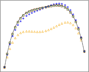
Shown in figure 1 are the profiles of density, velocity, temperature and errors in temperature for the two sets of simulations with different temperature variations. To demonstrate the effects of the various moments in the force term, simulations were performed with the force term expanded to orders corresponding to  $N = 0$, $1$, and $2$ in (2.7). In addition, the cases of $N=2$ were run with and without the contributions of $\boldsymbol {\sigma }$ in (2.20). As the reference solution, a high-resolution ( $N=450$) finite-difference results are also shown. We first note that due to the presence of cross-flow gravity and temperature gradient, the density and temperature are asymmetric. The velocity peak is also less than $U_c$ and does not occur at the centre. These effects are stronger in the cases with larger temperature variation.

Figure 1. Compressible Poiseuille flow with cross-flow gravity and heat gradient. Shown are profiles of density (a,b), velocity (c,d), temperature (e,f) and errors in temperature (g,h) as computed by the force term expanded to orders corresponding to  $N=0$, $1$ and $2$ in (2.7). The reference is a high-precision finite-difference solution which is also shown. In the left column shows the results for $\theta _b = 1.0$, $\theta _t = 1.1$, corresponding to a 10 % total temperature variation, and in the right column are those for $\theta _b = 0.7$, $\theta _t = 1.4$, corresponding to a 100 % total temperature variation.
Consistent with the theoretical analysis that the second-order ( $N=1$) force term is necessary in recovering the momentum equation and conservation of internal energy, it is evident from simulation results that retaining only the first-order force term ( $N=0$) causes significant overall discrepancies. The common second-order ( $N=1$) approximation yields satisfactory results for density and velocity, in accordance with the theoretical prediction of (2.23). However, noticeable differences with the reference solutions appear in the temperature profile and are more pronounced in the large temperature-variation cases. This discrepancy is eliminated in the third-order ( $N=2$) solutions, confirming the correctness and necessity of the third-order contribution by (2.20). Moreover, the contribution of the deviatoric tensor to the force term appears to be negligible in all cases tested, confirming the Chapman–Enskog analysis in the previous section.
3.2. Heat transfer between concentric cylinders under centrifugal force
The second test is the two-dimensional heat transfer between two concentric cylinders maintained at different temperatures and rotating with the same angular speed,  $\alpha$. In the rotating reference frame, the fluid is assumed static and subject to the centripetal acceleration of $\alpha ^2R$ where $R$ is the radial coordinate. The Navier–Stokes–Fourier equations have the following one-dimensional solution:
 \begin{equation} \theta = \theta_i + (\theta_{o}-\theta_i)\frac{\ln{R/R_i}}{\ln{R_o/R_i}} \quad\mbox{and}\quad \rho =\frac{\rho_i\theta_i}{\theta}\exp\left[\int_{R_i}^R \frac{\alpha^2r}{\theta(r)}\, {\rm d} r\right], \end{equation}
where  $\rho$ and $\theta$ are density and temperature, respectively, the subscripts $i$ and $o$ denote values at the inner and outer cylinders. The reference solution of density is solved by a high-precision numerical integration. Required the average of density $\bar {\rho } = \rho _0$, the $\rho _i$ is obtained by integrating the density in the whole domain.
The LBM simulations were performed on a  $L\times L$ lattice where $L=250$. The radial centripetal acceleration is $-\alpha ^2R$. The radius ratio $R_o/R_i$ is set to 5 with $R_o=Lc/2$. Using the width of the annular, $R_o-R_i$, as the characteristic length and the centreline velocity, $U_c\equiv \alpha (R_o + R_i)/2$, as the characteristic speed, the Reynolds number is defined as $Re = \rho _0\alpha (R_o^2-R_i^2)/2\mu$ where $\mu$ is the dynamic viscosity. As in the previous case, the relaxation time is set to $\tau =\mu /\rho \theta$ so that $\mu$ is a constant. Note that the fluid is static, and the centreline velocity, $U_c$, measures the compressibility as the isothermal Mach number, and the Reynolds number only plays the role of a dimensionless viscosity. As there is no flow in the rotating frame, all quantities are insensitive to the Reynolds number.
Shown in figure 2 are the radial profiles of density, temperature and the associated errors as computed with the force term expanded to various orders. The parameters are  ${Re = 100}$, $U_c = 0.3$ and $\rho _0=1$. Two simulations were performed for $\theta _i=1$, $\theta _o=1.1$ and for $\theta _i=1.4$, $\theta _o=0.7$. Note that the first and second expansions are identical as $\boldsymbol {u} = 0$ in this case. To be seen is that if the third-moment contribution is omitted, the errors in temperature profile is significant especially in the larger-temperature-variation case. It is also evident from the results that the third-order contribution is necessary to correctly recover the energy equation. The contribution of the stress tensor, $\boldsymbol {\sigma }$, vanishes as $\boldsymbol {\sigma }$ itself vanishes in the absence of fluid flow. In addition, as shown by (2.8), the $N=1$ terms vanish for continuity and momentum equations in absence of flow, which explains the observation that results for $N=0$ and $N=1$ are identical.

Figure 2. Heat conduction between two rotating concentric cylinders. Shown are the radial profiles of density and temperature and the associated errors computed with the force terms expanded to various orders. The superscript  $a$ denotes the analytical solutions. The left column shows the result for $\theta _i=1$, $\theta _o=1.1$, and the right column shows the result for $\theta _i=1.4$, $\theta _o=0.7$.
4. Conclusion
In summary, we have given a generic approach of incorporating body force in the LBM based on the Hermite expansion of the force term in the Boltzmann equation. In particular, a novel LBM forcing scheme for thermal compressible flows with second-order time accuracy has been obtained which includes the third-order contribution of the force term. The errors caused by the omission of this correction in common practices has been identified with an error in heat flux via Chapman–Enskog analysis. All theoretical findings, including the correctness and necessity of the new forcing term, have been confirmed numerically.
We note that the present approach is independent of the form of the equilibrium distribution nor the underlying lattice, and can be straightforwardly extended to include higher moments which are significant in non-equilibrium flows. Although for simplicity, we used the BGK collision model in present work. It is also straightforward to adapt it to more complicated collision models such as the spectral multiple relaxation time model.
Funding
This work was supported by the National Natural Science Foundation of China grant 92152107, Dept. of Science and Technology of Guangdong Province grant 2020B1212030001 and Shenzhen Science and Technology Program grant KQTD20180411143441009.
Declaration of interests
The authors report no conflict of interest.


