


1. Introduction
The dynamics of drops and bubbles in flowing dispersions has been a primary interest of researchers ever since the appearance of the pioneering works of Taylor (Reference Taylor1932, Reference Taylor1934) almost a century ago. Much attention was devoted to the deformation of such fluid particles because of its importance in systems involving interfacial transport and reactions that are common, e.g. in medical processes, food production and the chemical industry. Nevertheless, understanding patterns of deformation is also of interest in studies of basic fluid mechanics where applied mathematics methods are used, since nonlinearity and solution multiplicity are encountered in problems that can be superficially regarded as linear.
A considerable portion of attention was devoted to dilute multiphase systems containing non-interacting small drops and bubbles embedded in a flowing viscous fluid. In such dispersions, inertia forces on the dispersed bodies can be neglected and the small scale of the fluid particle permits a linearization of the macroscopic flow field acting on it. With these approximations, and with the absence of body forces, the main parameter controlling the deformation is the capillary number, Ca. Studies involved perturbation methods, slender body theory and numerical approaches, that were applied to Newtonian and non-Newtonian systems in which various forcing fields, such as uniform and linear flows, induce the deformation.
In view of the existing huge body of published material, with various directions of relevance, only some leading relevant analyses are mentioned below. More literature on the subject can be found in comprehensive reviews by Rallison (Reference Rallison1984) and Stone (Reference Stone1994). The deformation of a drop when Ca is small was studied by Cox (Reference Cox1969) and by Frankel & Acrivos (Reference Frankel and Acrivos1970) who used a first-order asymptotic expansion method. Barthes-Biesel & Acrivos (Reference Barthes-Biesel and Acrivos1973) extended the asymptotic approach to a second-order expansion in Ca. When the capillary number is relatively large and large deformations are expected, elongated bodies were studied by Buckmaster (Reference Buckmaster1972, Reference Buckmaster1973) and by Acrivos & Lo (Reference Acrivos and Lo1978) for drops and bubbles embedded in an extensional flow, where slender body theory was applied, and by Hinch & Acrivos (Reference Hinch and Acrivos1980) for a drop deformed in a shear field. In cases involving Ca that is not extremely large or small, the general approach is to use numerical methods such as finite difference, finite elements and level set. For a drop deforming in creeping flow of a viscous fluid, one of the most celebrated methods is the use of the boundary integral equation (BIE), developed by Rallison & Acrivos (Reference Rallison and Acrivos1978), following the earlier analysis by Ladyzhenskaya (Reference Ladyzhenskaya1969). This equation has been a starting tool for many analyses to follow.
When a viscous drop, initially spherical at rest, is deforming in an extensional or a shear flow the works of Taylor (Reference Taylor1932), Rallison & Acrivos (Reference Rallison and Acrivos1978) and Hinch & Acrivos (Reference Hinch and Acrivos1980) suggest that, with increasing flow rate, the drop can reach a critical shape at which it loses its stable form and beyond which its shape becomes unstable in the flow. A similar transition is found by Acrivos & Lo (Reference Acrivos and Lo1978) for a slender body in extensional flow where more than one branch of the solution of the equations of motion and more than one stationary shape, stable and unstable, are reported for a given capillary number.
It should be noted that multiple shapes of deformations of drops in extensional and shear flows are also encountered when the drops are non-Newtonian, e.g. having a power-law rheology (see Favelukis, Lavrenteva & Nir (Reference Favelukis, Lavrenteva and Nir2005, Reference Favelukis, Lavrenteva and Nir2006), in extensional flow and Favelukis & Nir (Reference Favelukis and Nir2016), in shear flow). In the former cases, lobes of solutions, containing multiple branches with only one of them stable, were predicted.
Recently, the multiplicity of such deformed stationary shapes was also reported for drops deforming in a linear compressional flow (Zabarankin et al. Reference Zabarankin, Lavrenteva, Smagin and Nir2013; Zabarankin, Lavrenteva & Nir Reference Zabarankin, Lavrenteva and Nir2015; Ee et al. Reference Ee, Lavrenteva, Smagin and Nir2018). There, the reported branches of solution were either stable stationary flat drops or unstable yet stationary toroidal drops. These predictions comprise dual branches of stationary solutions resulting for a given Ca, and they appeared to be unconnected. Similar shapes, flat and toroidal, are also reported by Fontelos, Garcia-Garrido & Kindelan (Reference Fontelos, Garcia-Garrido and Kindelan2011) for drops deforming in rotational flow field. There, the stationary branches of flat and toroidal drops are connected by a branch of flat discs having ever growing dimples.
The possible connection between the stationary flat and toroidal branches of drops deforming in compressional flow, by a branch of flat discs having ever growing dimples, is one of the subjects of this work. We aim to demonstrate it by suggesting approximate solutions that agree well with available numerical data for stationary stable (flat) and unstable (toroidal) drops and apply it to the connecting branch where exact numerical solutions are difficult to obtain. In § 2 we state the problem of a drop deforming in a compressional flow field (bi-axial extension), and the principal results are revisited and discussed. In § 3 we propose an approximate approach to construct branches of stationary shapes that would connect the flat and toroidal drops reported by Zabarankin et al. (Reference Zabarankin, Lavrenteva, Smagin and Nir2013, Reference Zabarankin, Lavrenteva and Nir2015) and by Ee et al. (Reference Ee, Lavrenteva, Smagin and Nir2018). A discussion of the results is given in § 4.
2. Drops in compressional flow, revisited
Consider a spherical drop of radius  ${a_1}$ and viscosity μ* to be embedded and deformed in an unbounded compressional viscous flow. The outer fluid viscosity is μ, and the viscosity ratio is denoted by λ = μ*/μ. It is assumed that both fluids have equal density and that they are immiscible. The surrounding fluid, in the absence of the drop, is subject to an undisturbed linear flow
 \begin{equation}u_i^\infty = {G_{ij}}{x_j}.\end{equation}
Here, the shear rate tensor  $\boldsymbol{\mathsf{G}}$ is constant and is given by ${G_{11}} = {G_{22}} = G,\;{G_{33}} ={-} 2G$ and ${G_{ij}} = 0\;\textrm{when}\;i \ne j$, with G > 0 being a constant characterizing the flow intensity.
Let V* denote the closed domain occupied by the drop, V the open domain occupied by the ambient fluid with S being the interface between them. Let the velocity and pressure fields in V and V* be denoted as u, p and u*, p*, respectively. As we assume creeping flow conditions, these fields satisfy the stationary Stokes equations
 \begin{equation}\frac{{\partial {\sigma _{ij}}}}{{\partial {x_j}}} = 0,\quad \frac{{\partial {u_j}}}{{\partial {x_j}}} = 0\quad \textrm{in}\;V\quad \textrm{and}\quad \frac{{\partial \sigma _{ij}^\ast }}{{\partial {x_j}}} = 0,\quad \frac{{\partial u_j^\ast }}{{\partial {x_j}}} = 0\;\textrm{in}\;{V^\ast },\end{equation}
where  ${\sigma _{ij}} ={-} p{\delta _{ij}} + \mu (\partial {u_i}/\partial {x_j} + \partial {u_j}/\partial {x_i})$ and with a similar expression in V*.
The velocity is continuous at the interface
 \begin{equation}{u_i} = u_i^\ast \;\textrm{on}\;S,\end{equation}
while at infinity  ${u_i} = u_i^\infty $ and $p = 0$.
The stress balance across the interface is of the form
 \begin{equation}({\sigma _{ij}} - \sigma _{ij}^\ast ){n_j} = \gamma \frac{{\partial {n_j}}}{{\partial {x_j}}}{n_i}\;\textrm{on}\;S,\end{equation}
with the interfacial tension  $\gamma $ being constant. Here, n is a unit normal pointing outward into the ambient phase and $\boldsymbol{\nabla }\boldsymbol{\cdot }\boldsymbol{n}$ is the surface curvature. The kinematic condition denoting the surface deformation is given by
 \begin{equation}{U_n} = {u_n}\;\textrm{on}\;S.\end{equation}
For a given shape of the drop, the stationary Stokes equations (2.2a,b) with boundary conditions (2.3) and (2.4) can be reduced to a system of integral equations for the surface of the viscous drop, S. In the particular case of equal viscosity of the phases these reduce to the explicit expression
 \begin{equation}{u_i}(\boldsymbol{x}) = u_i^\infty (\boldsymbol{x}) - \frac{\gamma }{{2\mu G{a_1}}}\mathop{{\int\!\!\!\!\!\int}\mkern-21mu {\bigcirc}}\nolimits_S {{J_{ij}}(\boldsymbol{x} - \boldsymbol{y}){n_j}(\boldsymbol{y})} \frac{{\partial {n_k}}}{{\partial {x_k}}}(\boldsymbol{y})\,\textrm{d}S,\;\end{equation}
where the kernels are given by
 \begin{equation}{J_{ij}}(\boldsymbol{r}) = \frac{1}{{4{\rm \pi}}}\left( {\frac{{{\delta_{ij}}}}{{|\boldsymbol{r}|}} + \frac{{{r_i}{r_j}}}{{|\boldsymbol{r}{|^3}}}} \right).\end{equation}
 In what follows, throughout the paper, the length and the velocity and pressure fields are scaled with a 1,  $G{a_1}$ and μG, respectively, and the capillary number, Ca, is defined to be $Ca = \mu G{a_1}/\gamma $. The dimensionless form of (2.6), keeping the respective nomenclature for the sake of brevity, is
 \begin{equation}{u_i}(\boldsymbol{x}) = u_i^\infty (\boldsymbol{x}) - \frac{1}{{2Ca}}\mathop{{\int\!\!\!\!\!\int}\mkern-21mu {\bigcirc}}\nolimits_{{S_y}} {{J_{ij}}(\boldsymbol{x} - \boldsymbol{y}){n_j}(\boldsymbol{y})} \frac{{\partial {n_k}}}{{\partial {x_k}}}(\boldsymbol{y})\,\textrm{d}{S_y}.\end{equation}
 Given the axial symmetry of the drop under consideration, a cylindrical coordinate system (r, φ, z) with basis (er, eφ, ez) is used with the z-axis coinciding with the x 3-axis defined following (2.1). In this coordinate system, the undisturbed flow velocity is given by  ${\boldsymbol{u}^\infty } = r{\boldsymbol{e}_r} - 2z{\boldsymbol{e}_z}$, and G = 1 can be assumed without loss of generality. Furthermore, the integral equations (2.6) are integrated over the angular coordinate, φ, and are reduced to expressions containing curvilinear integrals over the cross-section of the drop interface S. The resulting expressions for the kernels can be found e.g. in Pozrikidis (Reference Pozrikidis1992).
At each time step, the unit normal to the surface and the surface curvature are calculated numerically from the newly established surface points after the quasi-steady progress. Detailed descriptions are given by Zabarankin et al. (Reference Zabarankin, Lavrenteva, Smagin and Nir2013, Reference Zabarankin, Lavrenteva and Nir2015) and by Ee et al. (Reference Ee, Lavrenteva, Smagin and Nir2018).
The algorithm for obtaining the steady shapes, employed by Zabarankin et al. (Reference Zabarankin, Lavrenteva, Smagin and Nir2013), was to start the solution from a spherical shape and proceed by deforming the shape in a quasi-steady manner in the direction of  ${U_n}$ until ${U_n} = 0$ was established to a desired degree of accuracy. The obtained singly connected stationary shapes do not change for an indefinitely long time and they are addressed as stable. These shapes vary between a sphere at Ca = 0, via nearly oval shapes at intermediate values of Ca, to flattened shapes at higher values of Ca, until a critical solution is reached at Ca = Cacr for each value of the viscosity ratio beyond which stable shapes were not found.
The algorithm for obtaining the toroidal stationary shapes, used by Zabarankin et al. (Reference Zabarankin, Lavrenteva and Nir2015) and by Ee et al. (Reference Ee, Lavrenteva, Smagin and Nir2018), was to start from a torus with a circular cross-section and a finite major radius, R, and solve problem (2.1)–(2.5) (or the equivalent problem (2.6) and (2.7) for the velocities at the interface). The consequential deformation is then followed quasi-steadily in the direction of  ${U_n}$. It was demonstrated that when the torus R is small, the torus collapses to the axis, while for higher values of R, it expands indefinitely. When R belongs to a certain interval, the shape stays visually unchanged for a relatively long time. The value of R that yields the longest duration of stationary deformed toroidal shape with $||{U_n}||\ll 1$, both established to a desired degree of accuracy, is termed Rcr and the yielded shape is accepted as a stationary solution. These toroidal shapes are unstable and, with the passage of time, they either collapse or expand due to unavoidable numerical disturbances. These shapes vary from a torus of infinite extent with a circular cross-section at Ca = 0, via tori with finite radii having nearly oval cross-sections at intermediate Ca (e.g. around the minimum of the upper curve in figure 1), to tori with shrinking inner radius at higher values of Ca having cross-sections with an egg shape, until a solution of an almost totally collapsed shape is reached at Ca ~ Cacr for each λ, beyond which stationary shapes could not be numerically established.

Figure 1. Deformation of a drop in compressional (bi-extensional) viscous flow, λ = 1. (Zabarankin et al. Reference Zabarankin, Lavrenteva and Nir2015).
Axisymmetric deformation patterns are depicted in figure 1 for equal viscosity ratio, λ = 1, where the stationary deformations, denoted by a Taylor deformation parameter, defined as
 \begin{equation}D = \frac{{{R_{max}} - {z_{max}}}}{{{R_{max}} + {z_{max}}}},\end{equation}
are displayed as function of the capillary number, Ca. Here, Rmax and zmax denote the maximum distance of the drop surface to the axis of symmetry and half the maximum thickness of the drop, respectively, and the solid curves correspond to steady singly connected shapes, while the dashed curves denote stationary toroidal shapes. These are actually two branches of the solution of problem defined by (2.1)–(2.5) with  ${U_n} = 0$.
Some characteristics of the system described above deserve further attention. All steady branches lose their stability at critical points, Cacr, where the rate of change of the deformation parameter with Ca becomes infinite. These critical values depend on the viscosity ratio λ. However, the critical deformation parameter and the drop dimensions appear to be similar for all viscosity ratios, with the only difference between small λ and λ ≥ O(1) is the development of small dimples near the axis of symmetry in the latter cases. These critical Taylor deformation parameters are all near 0.75, indicating that flat drops in compressional flow cannot become really thin, opposite to the deformation of low viscosity drops in extensional flow that can become really slender.
While for the simply connected stable solution, it was possible to determine the critical points numerically, for the toroidal drops it was not possible to do so with a satisfactory degree of accuracy. As described above, the stationary solutions were determined when the toroidal deformation became steady for an extended stretch of time, before the loss of stability due to unavoidable numerical disturbances, after starting the process with a circular cross-section and a radius R = Rc. However, as the stationary shape of the torus became close to a complete collapse, these stretches of time became shorter and shorter. Thus, the deformation curves for these cases were stopped at capillary numbers slightly below Cacr with the latter values only estimated also close to 0.75.
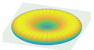
In spite of the similarity of the near critical values of deformation, the two branches, for a given λ, are not connected. There is also a shape gap for the corresponding cases of λ. The simply connected flat drops at Cacr are not completely collapsed, nor are the toroidal drops at Ca near the critical one. A calculation of the surface evolution of the flat drops at Cacr suggests a family of dynamically (not stationary) evolving shapes, with ever increasing dimples around the axis of symmetry, as are depicted in figure 2. Similar dynamic shapes were reported in Stone & Leal (Reference Stone and Leal1989). Once the dimples touch each other, two families of shapes can evolve, as discussed by Fontelos et al. (Reference Fontelos, Garcia-Garrido and Kindelan2011). Toroidal (I), in the shape of rings, and toroidal (II) having an inner thin layer of the drop fluid at and around z = 0. The latter tori (II) are not the subject of this paper and, thus, we assume that, once the dimples touch each other at z = 0, a torus of type (I) is formed. The existence of a branch of stationary, yet unstable, solutions to (2.1)–(2.5), possibly connecting the stable flat drops branch and the one of unstable tori, is one of the main objectives of this paper. However, it was not possible to achieve such stationary solutions by direct numerical approach because of the unstable nature of the dimpled flat shapes with the dimples dynamically collapsing to form tori. Thus, an approximate approach is used to estimate this branch as well as the numerically obtained flat and toroidal shapes.

Figure 2. Shapes in dynamic evolution of an unstable drop. Here, λ = 1 and Ca = 0.2, slightly exceeding the critical capillary number estimated at Cacr ≈ 0.197. Time, t, is normalized by G −1.
3. Approximate solutions
A sphere embedded in compressional flow is the zero-order approximation of the shape of a singly connected drop when the capillary number is near 0. Indeed, when  $Ca \ll 1$, this spherical shape can be accepted for further applications. If Ca is slightly increased, asymptotic expansions were used to estimate the deformation of the drop in terms of spherical harmonics. The O(Ca) theory shows that the drop deforms into an ellipsoid (see e.g. Leal Reference Leal1992). The formal use of the obtained formula for large perturbations predicts a breakup of the drop at $C{a_{cr}} = 4(1 + \lambda )/(16 + 19\lambda )\sim 0.229$ for λ = 1, while for the O(Ca 2) the deformation in axisymmetric compression. Barthes-Biesel & Acrivos (Reference Barthes-Biesel and Acrivos1973) reported $C{a_{cr}} = 0.13$ at this viscosity ratio. Both are not close to the value $C{a_{cr}} = 0.197$ obtained numerically by Zabarankin et al. (Reference Zabarankin, Lavrenteva, Smagin and Nir2013). When Ca is further increased and the drop assumes a shape close to an oblate spheroid or flat disc, approaching the critical stable form, the deformation can be approximated using some empirical expressions which are a generalization of the spheroidal shape, or by series expansions using, e.g. Chebyshev polynomials. Such approximations are described in Zabarankin et al. (Reference Zabarankin, Lavrenteva, Smagin and Nir2013), where comparisons are made with actual numerically calculated shapes emerging from solution of (2.1)–(2.5). The shapes, spherical and oval, are attractive for use since problems for these assumed shapes can be formulated and solved without resorting to elaborated numerical procedures.
Similarly, for toroidal drops, approximations of simple cross-sectional shapes, such as circular or elliptical, are also attractive. Zabarankin (Reference Zabarankin2016, Reference Zabarankin2019) derived and solved the problem of a toroidal drop having circular and elliptical sections, respectively. In these papers, he used conformal mapping techniques to solve the equations of motion for the predetermined cross-sectional shapes. With this approach one must suggest an artificial criterion for stationarity, such as a minimum of some norm of the normal velocity at the interface or immobility of an identified point on the circle or the ellipse. Of course, a constant volume stationary torus with circular cross-section exists only when Ca → 0 and when extension is R → ∞. When R is arbitrary, considerable deviations from actual stationary shapes exist and a normal velocity at the surface appears. Indeed, Zabarankin (Reference Zabarankin2016) calculated such normal velocity profiles along the surface S. When Ca increases slightly but is still very small, the approximation is good, but any further increase of Ca yields deviations from the actual cross-sectional shape and results in the appearance of normal velocity components on S, which he calculated and displayed. For toroidal drops with cross-sectional shapes that cannot be described as close to elliptical, Zabarankin et al. (Reference Zabarankin, Lavrenteva and Nir2015) suggested expansions in Chebyshev polynomial that yielded shapes close to the numerically calculated ones.
In this section we aim to obtain an approximation to stationary shapes that spans the already available flat and toroidal solutions, and also the highly unstable shapes in the interval between the point of loss of stability of the flat singly connected drop (e.g. at Ca ≈ 0.197 for λ = 1) and the point of total collapse of toroidal drops (at Ca > 0.19). In view of the dynamics described in figure 2, these solutions are expected to be highly unstable, with the flat shapes showing ever growing dimples until the collapse toward a toroidal shape is achieved. In this interval 0.19 < Ca ≤ 0.197 one expects to find dual solutions, stable and unstable, to singly connected drops with a lower deformation factor for the stable branch and a higher factor for the unstable ones. An algorithm to achieve this dual-solution state is to extend the finite element description of the surface, with the number of surface points spanning 200 < N < 2000, substitute it into the BIE (6 or 8) and minimize a measure of the residual non-zero normal component of the surface velocity. This algorithm would become an optimization problem with respect to N parameters, hence a tedious procedure. An alternative algorithm is to assume an approximate description of the surface involving a known family of shapes, as was described above with the approximations of circular and elliptical cross-sections used by Zabarankin (Reference Zabarankin2016, Reference Zabarankin2019), and perform a similar yet less laborious optimization procedure with a much smaller number of parameters. The latter algorithm is adopted here and is described below.
We examine a solution of compressional Stokes flow about a stationary axisymmetric drop of a given volume embedded in its origin. The shape of the drop is assumed to belong to some m parametric family. For given values of these parameters, the shape is discretized. Further, unit normal and curvature are calculated and these are substituted in the BIE (2.6) or (2.8). To improve the accuracy of computation of the involved singular integrals, use is made of the singularity subtraction method (see e.g. Pozrikidis Reference Pozrikidis1992). Surface integrals are reduced to contour ones, taking into account the axial symmetry of the problem and integrating over the angle. All the integrands are expressed analytically via special functions. Numerical integration was performed with a second-order algorithm and 2000 intervals.
As a result, because the shape is only an approximation and is not an exact stationary solution, a normal velocity component,  ${U_n}$, results over the surface that depends on m + 1 parameters (m parameter description of the shape and the capillary number, Ca). Stationarity is defined if an average norm of ${U_n}$ is minimized. Note that, since the shape is only approximation, the minimum of the norm is not expected to be zero.
In this study, we have used the norm of Hilbert space L 2 of the interfacial velocity divided by the surface area and define function to be minimized as
 \begin{equation}||{U_n}|{|^2} = {{\mathop{{\int\!\!\!\!\!\int}\mkern-21mu {\bigcirc}}\nolimits_S {U_n^2\,\textrm{d}s} } / S} = {{\int_l {rU_n^2\,\textrm{d}l} } / {\int_l {r\,\textrm{d}l} }}.\end{equation}
 Note that the number of independent parameters in the used approximations below is reduced by the constraint that the volume remains constant, i.e.  $4{\rm \pi}/3$. There are three algorithms that can be applied for the minimization process. Stationarity can be defined by minimizing (3.1) for a given Ca (defined as method M1). This can be achieved by applying an inverse method, where Ca is determined by a particular choice of conditions at some surface points, for example, by the choosing one of the m parameters and requiring that the normal velocity at r = Rmax and z = 0 vanish, which implies that the oval radial dimension does not change (defined as method M2). Of course, the latter choice is rather arbitrary and not unique as most other surface points are not immobile and will tend to deform the oval along the resulting local non-zero normal velocity component. Yet another inverse method (defined here as M3), suggested in Zabarankin et al. (Reference Zabarankin, Lavrenteva, Smagin and Nir2013), considers only one of the shape parameters being fixed and all others (including Ca) as independent parameters. The inverse methods require considerably less computational effort than M1 due to the simple (quadratic) dependence of the velocity at the interface and of the functional (3.1) on 1/Ca. For M2 in the case λ = 1, the capillary number is found as
 \begin{equation}Ca = \frac{1}{{2{R_{max}}}}\mathop{{\int\!\!\!\!\!\int}\mkern-21mu {\bigcirc}}\nolimits_{{S_y}} {{J_{ij}}({\boldsymbol{x}_m} - \boldsymbol{y}){n_j}(\boldsymbol{y})} \frac{{\partial {n_k}}}{{\partial {x_k}}}(\boldsymbol{y})\,\textrm{d}{S_y},\end{equation}
where xm = (Rmax, 0) in a cylindrical coordinate system. For M3 in the case λ = 1,
 \begin{equation}Ca = \frac{\displaystyle{{{\mathop{{\int\!\!\!\!\!\int}\mkern-21mu {\bigcirc}}\nolimits_{{S_x}} {\left( {{n_i}(\boldsymbol{x})\mathop{{\int\!\!\!\!\!\int}\mkern-21mu {\bigcirc}}\nolimits_{{S_y}} {{J_{ij}}(\boldsymbol{x} - \boldsymbol{y}){n_j}(\boldsymbol{y})} \frac{{\partial {n_k}}}{{\partial {x_k}}}(\boldsymbol{y})\,\textrm{d}{S_y}} \right)} }^2}\,\textrm{d}{S_x}}}{\displaystyle{2\mathop{{\int\!\!\!\!\!\int}\mkern-21mu {\bigcirc}}\nolimits_{{S_x}} {({n_i}(\boldsymbol{x})u_i^\infty )\left( {{n_i}(\boldsymbol{x})\mathop{{\int\!\!\!\!\!\int}\mkern-21mu {\bigcirc}}\nolimits_{{S_y}} {{J_{ij}}(\boldsymbol{x} - \boldsymbol{y}){n_j}(\boldsymbol{y})} \frac{{\partial {n_k}}}{{\partial {x_k}}}(\boldsymbol{y})\,\textrm{d}{S_y}} \right)\,} \textrm{d}{S_x}}}.\end{equation}
Below, in what follows, we have used all three minimization methods and compared the resulting deformations and shapes. We examine the applicability of a range of low parametric approximations with m = 2, 3 and 4, for the case λ = 1, in which case (2.8) and associated shape parameters (e.g. unit normal, curvature) are used to calculate the residual norm given in (3.1). Minimization of a function (3.1) was performed numerically making use of the Matlab function fmincon with the internal point algorithm. In what follows, we term the shapes obtained by this procedure ‘stationary’. The obtained results are compared to the previously obtained numerical ones. The approximate shapes that are close to stable (in the sense of § 2) are addressed to as ‘stable’. All the others are termed ‘unstable’.
3.1. Cassini ovals, m = 2
Consider the family of shapes known as Cassini ovals (see e.g. Boyadzhiev & Boyadzhiev Reference Boyadzhiev and Boyadzhiev2018). A common representation of these two-dimensional (2-D) ovals is of the Cartesian form
 \begin{equation}{[{(ax)^2} + {(ay)^2} + 1]^2} - 4{(ax)^2} = {\varepsilon ^4},\end{equation}
where a and ε are constants. The oval is the locus of points (x, y) with distances to two focal points located at (−1/a,0) and (1/a,0) having a constant product (ε a)2. There are some interesting combinations of a and ε. When a→∞ the two focal points collapse to the origin and the oval is a circle. When ε = √2 the oval has a flat form just before the appearance of dimples at the centre x = 0. The special transition case, ε = 1, is known as the lemniscate of Bernoulli, where the point (0,0) is joint to two touching ovals, and cases with ε < 1 yield two separated symmetric ovals on both sides of x = 0.
If (x, y) is replaced by (r, z) and the 2-D domain is rotated about the z axis the four cases above describe a sphere, a flat drop, a drop collapsed at the centre and a toroidal body. Hence, the Cassini rotated oval with two parameters has shapes similar to the two branches of the drop deforming in a compressional flow (as shown in figure 1), which are connected continuously and uniformly, by a segment depicting flat shapes with ever increasing surface dimples at the axis of symmetry. The fixed volume condition results in an explicit relation between a and ε, a = a(ε). If V(a, ε) is a volume of rotated Cassini oval defined by (3.4), then for  $a(\varepsilon ) = {(4{\rm \pi}/3V(1,\varepsilon ))^{1/3}}$, $V(a(\varepsilon ),\varepsilon ) = 4{\rm \pi}/3$. Graphical presentations of the various cases of Cassini ovals can be found in Wikipedia, in Wolfram MathWorld or in Boyadzhiev & Boyadzhiev (Reference Boyadzhiev and Boyadzhiev2018).
As a first approximation, we used the ovals (3.4) with a = a(ε) and looked for parameter ε to minimize (3.1) for a given Ca (M1 method). The results are summarized in table 1, where ε (Ca), a(ε (Ca)) and  $||{U_n}|{|^2}$ defined by (3.1) are presented. It was found that, at any Ca, the function (3.1) has two minima, one with ε > 1 and another with ε < 1, describing singly connected and toroidal shapes, respectively. For both shapes, ε approaches 1 as Ca increases, but no critical or maximal value for Ca is observed. The residual values of the functional ≤ O(10−1) only for singly connected shapes and Ca ≤ 0.01. The deformation curve corresponding to the obtained shapes, shown in figure 3 by dashed lines, are compared to the numerical results of Zabarankin et al. (Reference Zabarankin, Lavrenteva, Smagin and Nir2013, Reference Zabarankin, Lavrenteva and Nir2015) shown by the solid curves. Obviously, for this initial crude m = 2 approximation, the deformation curve is far from the numerical calculations. For singly connected drops the approximation obtained by the M1 method is close to the numerical one only for Ca < 0.1, while for higher Ca, the deformation is underestimated by this method. For toroidal shapes, considerable underestimation of drop deformation is observed for all values of the capillary number. Another deviation is characterized by erroneous results obtained for Ca larger than the critical one obtained numerically by Zabarankin et al. (Reference Zabarankin, Lavrenteva and Nir2015) (Cacr = 0.197) as is shown in the case Ca = 0.25 in table 1.

Figure 3. Deformation curve of a drop in compressional (bi-extensional) viscous flow, obtained by two-parameter model, λ = 1. Dashed-dotted curves – minimization of functional (3.1) (method M1). Solid curves – condition Un(Rmax) = 0 (M2). Dashed curves – (M3). Marked curves – numerical computations (Zabarankin et al. Reference Zabarankin, Lavrenteva and Nir2015).
Table 1. Parameters of the ‘stationary’ Cassini ovals (3.4) found from the minimization of (3.1) for various given capillary numbers (method M1) and the corresponding minimum values of (3.1).

The inverse methods (M2) and (M3) in the case of two parametric models with a volume conservation condition lead to an explicit expressions Ca = Ca 2(ε) and Ca = Ca 3(ε), respectively. These functions achieve maximum at some ε > 1, which can be attributed as a critical capillary number for this m = 2 approximation. Table 2 presents a(ε), Ca 2(ε), Ca 3(ε) and corresponding values of the functional  $||{U_n}|{|^2}$ defined by (3.4).
Table 2. Parameters of the ‘stationary’ Cassini ovals (3.4) found by the inverse methods M2 and M3 with corresponding values of Ca and the functional (3.1).

The deformation curves computed with methods M2 and M3 are shown in figure 3 by dotted and dashed-dotted curves, respectively. The existence of the critical Ca reflects qualitative features of the results by Zabarankin et al. (Reference Zabarankin, Lavrenteva, Smagin and Nir2013, Reference Zabarankin, Lavrenteva and Nir2015). However, the deformation curves corresponding to these shapes differ considerably from the numerically computed ones and the critical Ca is highly underestimated. One can observe that the M3 method, in which only one parameter was predetermined, provides a better, but not yet satisfactory, approximation of the deformation curve as well as of the critical capillary number. Note that the highest values of the minimized norm, calculated by (3.1), are obtained for a singly connected dimpled drop (ε > 1) near the estimated maximum Ca.
3.2. Extended Cassini ovals, m = 3
As a second approximation the ovals (3.4) are recast in the form
 \begin{equation}{[{(abr)^2} + {(az)^2} + 1]^2} - 4{(abr)^2} = {\varepsilon ^4},\end{equation}
and, in this reorganization, the Cassini rotated oval is slightly extended with one more independent parameter added, by choosing ε to be independent of a and b, and with the transition from singly connected rotated ovals to toroidal ones kept at ε = 1. The fixed volume condition results in an explicit relation between a, b and ε, a = a(ε,b). Table 3 presents the results of the minimization of (3.1) for ovals (3.5) with a = a(ε,b) with respect to ε and b. As in the previous case, two minima were found at any Ca, with ε > 1 and ε < 1, describing singly connected and toroidal shapes, respectively. The residual values of the functional are several orders of magnitude lower than those obtained for two parametric model described in the previous sub-section.
Table 3. Parameters of the ‘stationary’ extended Cassini ovals (3.5) found from the minimization of (3.1) for various capillary numbers (using method M1), and the minimum corresponding values of (3.1).

The deformation curves corresponding the shapes obtained by method M1, shown in figure 4 by dashed-dotted lines, are compared to the numerical results of Zabarankin et al. (Reference Zabarankin, Lavrenteva, Smagin and Nir2013, Reference Zabarankin, Lavrenteva and Nir2015), shown by diamonds and circles. Note that the deformation curve for singly connected drop obtained by the M1 method is close to the numerical one for Ca < 0.18, extending the corresponding approximation by (3.4), while for higher Ca, the deformation is underestimated by this method and, again as in the case m = 2, provides results for Ca that exceed the known critical Cacr = 0.197. Note also that the norm there is an order of magnitude higher. For toroidal shapes, the deformation curve follows the numerical one up to Ca ~ 0.08 while for higher Ca, an overestimation of drop deformation is observed. At Ca ~ 0.18, the deformation curve of M1 intersects the numerical one. The residual value of (3.1) has a minimum in the vicinity of this point.

Figure 4. A comparison of numerically calculated deformation values of stationary flat singly connected drop (lower diamonds) and toroidal drops (upper circles) with stationary solutions of extended Cassini rotated ovals defined by (3.5) all deformed in compressional flow, λ = 1. Dashed-dotted, solid and dashed curves are computed with methods M1, M2 and M3, respectively. Thick (blue) and thin (red) lines correspond to singly connected and toroidal shapes, respectively.
The results obtained by methods M2 (requiring  ${U_n}({R_{max}}) = 0$) and M3 (with considering Ca as an independent parameter for a given value ε) are presented in figure 4 by solid and dashed lines, respectively. For both methods, it is seen that three branches of solution are evident: a branch of stable flat drops, a branch of flat drops containing dimples and a branch of toroidal drops, all connected continuously. Furthermore, there appears to be a maximum value for Ca at which the rate of change of D is infinite, denoting the possible transition from stable flat shapes to unstable flat ones with dimples. Beyond this point until the point of transition to toroidal shapes, the minimization produces two minimum values of (3.1) for (3.5) with two flat singly connected shapes, the additional one exhibiting ever increasing dimples.
The values of parameters obtained by methods M2 and M3 and the residual values of the functional (3.1) are presented in table 4. In contrast to the two parametric model, here, the residual values resulting from the use of all three models are of the same order of magnitude. The deformation curves for flat drops nearly coincide with the one calculated numerically by Zabarankin et al. (Reference Zabarankin, Lavrenteva, Smagin and Nir2013) when the shapes are nearly spherical or spheroidal (Ca < 0.15). And they are close to this curve for Ca < 19. Also, for singly connected shapes, the deformation curves obtained by all three approximate methods nearly coincide for all values of the capillary number except for the vicinity of critical point. For Ca ≥ 0.18, method M2 slightly underestimates the deformation, while method M3 slightly overestimates it. The maximum value for Ca at which the rate of change of D is infinite, obtained with model M2, Ca = 0.1976, is surprisingly close to the critical Ca, obtained in numerical solution.
Table 4. Parameters of the ‘stationary’ extended Cassini ovals (3.5) found by the inverse methods M2 and M3 with corresponding obtained values of Ca, and the functional (3.1).

However, as is evident from comparison with the existing numerical results, the deformation results suggested by (3.5) deviate considerably from those calculated numerically by Zabarankin et al. (Reference Zabarankin, Lavrenteva and Nir2015) when Ca is higher than 0.18, and the deformation at near-critical capillary numbers is underestimated. For toroidal shapes, the deformation curves obtained the 3 parameter model deviates from numerical one already for Ca > 0.08 for all methods. Hence, the additions of one independent parameter in the Cassini rotated ovals, as described by (3.5), demonstrates qualitatively the expected behaviour but does not yield an acceptable approximation at intermediate and higher values of the capillary number, and in particular in the vicinity of the critical Ca and near the transition to toroidal shapes.
3.3. Generalized Cassini Rotated Ovals, m = 4
We extend our approximation by defining and introducing generalized Cassini rotated ovals of the following form:
 \begin{equation}{[{(abr)^{2\alpha }} + {(az)^2} + 1]^2} - 4{(abr)^{2\alpha }} = {\varepsilon ^4}.\end{equation}
Again, we require  $a = a(\varepsilon ,b,\alpha ) = {(4{{\rm \pi} /}3V(1,\varepsilon ,b,\alpha ))^{1/3}}$, with $V(a,\varepsilon ,b,\alpha )$ denoting the volume of the rotated oval (3.6) to ensure that the volume of (3.6) equals that of a unit sphere.
Here, the additional parameter α assists in bringing the oval shapes closer to the numerically calculated ones in the entire domain of Ca, while the transition from singly connected drops to toroidal ones is still kept at ε = 1. We have used all three definitions of stationarity, i.e. methods M1, M2 and M3. All three methods follow closely the numerically calculated results for the stable singly connected flat drop and the unstable toroidal one and are depicted in figure 5(a,b). The full diamonds and circular points are the numerical calculations of flat and toroidal drops from Zabarankin et al. (Reference Zabarankin, Lavrenteva, Smagin and Nir2013) and Zabarankin et al. (Reference Zabarankin, Lavrenteva and Nir2015), respectively. In figure 5(b) along the region of existing dual solutions, i.e. Ca < 0.197 for singly connected drops and Ca < 0.187 for toroidal bodies, we added some of the calculated points as hollow circles, stars and hollow squares showing several points calculated by methods M1, M2 and M3, respectively, taken from the tables of data below.

Figure 5. A comparison of deformation curves of stationary flat and toroidal drops, obtained by direct numerical solution, with stationary solutions of the generalized Cassini rotated ovals defined by (3.6), all deformed in compressional flow, λ = 1. Filled diamonds and circles – numerical results from Zabarankin et al. (Reference Zabarankin, Lavrenteva, Smagin and Nir2013, Reference Zabarankin, Lavrenteva and Nir2015). Dashed-dotted, dashed and solid curves – approximation by methods M1, M2 and M3, respectively. (a) Total deformation domain. A, B, C and D denote the location of spherical shape, critical steady flat shape, collapse from dimpled flat to toroidal shape and extended thin toroidal shapes, respectively. (b) Close up, enlarging region of transitions, with examples of data points for M1, M2 and M3 along the lines marked by hollow circles, stars and hollow squares, respectively.
The use of the generalized Cassini oval approximation reveals that the flat drop branch and the toroidal branch predicted by Zabarankin et al. (Reference Zabarankin, Lavrenteva, Smagin and Nir2013, Reference Zabarankin, Lavrenteva and Nir2015) and shown in figure 1, are extended beyond the available direct numerical solution of problem (2.1)–(2.5). It is shown that the approximated solution of (2.8) for the case of λ = 1 beyond the loss of stability of flat drops, at Cacr = 0.197, is connected to a branch of unstable stationary flat drops with ever growing dimples at their centre and with decreasing values of Ca. Thus, Cacr is also a maximum, and there exist dual solutions for Ca < Cacr. Similarly, the curve showing toroidal drops is also characterized by a maximum value of the capillary number, i.e. Cat ~ 0.187, and exhibits a similar additional solution there with the second one unveiling collapsing stationary tori that have a shrinking inner radius at ever decreasing Ca. The locations indicated by the letters A to D indicate the points of transition from one branch to another. The two additional branches meet at common Ca and deformation factors. Extrapolation of the curves to contact provides the values (Cam, Dm) = (0.181, 0.799), (0.182, 0.788) and (0.181, 0.794) for methods M1, M2 and M3, respectively.
It should be noted that the turning of the stationary solutions to exhibit multiplicity of deformation parameters and shapes upon approaching the critical Ca values, for both flat and toroidal drops, are characteristic to similar deformation patterns in viscous systems. Fontelos et al. (Reference Fontelos, Garcia-Garrido and Kindelan2011) studied the deformation of the drop undergoing a solid body rotation in a slightly lighter viscous fluid, demonstrating and extending the classical experiment of Plateau (Reference Plateau1857). Physically, their problem is quite close to that in our manuscript, while mathematically it can be reduced to ordinary differential equations and solved with very high accuracy. There, a similar system of branches was found. The point (Cam, Dm) is also the location of an additional bifurcation point where other drops of toroidal shape emerge (type II, as defined by Fontelos et al. Reference Fontelos, Garcia-Garrido and Kindelan2011). These are not the subject of this paper. It is interesting to note that for D < Dm there are 3 different regions of stationary solutions to (2.8). In the interval 0 < Ca < Cam there are two solutions, one unstable toroidal drop and one stable simply connected flat drop; in the interval Cam < Ca < Cat there are four solutions, one unstable dimpled flat drop, two unstable toroidal drops and one stable flat drop; and in Cat < Ca < Cacr we find two solutions of singly connected bodies, one unstable dimpled drop and one stable flat drop. This multiplicity of solutions, having a critical turning point, is not uncommon and appears in other problems with nonlinear characteristics in viscous flow (e.g. in addition to Fontelos et al. (Reference Fontelos, Garcia-Garrido and Kindelan2011), discussed above, see Acrivos & Lo (Reference Acrivos and Lo1978), Favelukis et al. (Reference Favelukis, Lavrenteva and Nir2005); for slender low viscosity Newtonian and power-law drops in extensional viscous flow, respectively). Note the difference of approximately 1.5% between the maximum value of Cat = 0.187, calculated by the approximation method, and the most extended point at Ca = 0.19 for toroidal drops, reported previously, by our group (Zabarankin et al. Reference Zabarankin, Lavrenteva and Nir2015). We comment that, in view of the method of determination of stationarity described by the latter (i.e. duration of stationarity in the dynamic evolution before losing stability), it is expected that the exact determination of the critical turning point of the toroidal branch by the numerical calculation can be biased, and some care should be exercised regarding its precise position.
The values of parameters obtained by methods M1, M2 and M3 and the residual values of the functional (3.1) are presented in tables 5, 6 and 7, respectively. The residual values resulting from the use of all three models are of the same order of magnitude and an order of magnitude lower than those of the 3-parametr model (m = 3) discussed in the previous section. All three methods yield results that nearly coincide with the ones calculated numerically by Zabarankin et al. (Reference Zabarankin, Lavrenteva, Smagin and Nir2013) for flat drops for all Ca ≤ 0.197, and by Zabarankin et al. (Reference Zabarankin, Lavrenteva and Nir2015) for toroidal drops for all Ca ≤ 0.18. Below the critical points, Cacr = 0.197 for flat drops and Cat = 0.187 for toroidal drops, and above the point of joining at Cam = 0.181, the three methods of approximation yield dual solutions expressed by two values of deformation in figure 5 and two values of ε (the thickness parameter in (3.6)) in the tables below.
Table 5. Parameters of the ‘stationary’ generalized Cassini ovals (3.6) found from the minimization of (3.1), using method M1, for various capillary numbers, and the corresponding minimum values of the norm (3.1).

Table 6. Parameters of the ‘stationary’ generalized Cassini ovals (3.6) found by the inverse method M2 with corresponding values of Ca and minimum values of the functional (3.1).

Table 7. Parameters of the ‘stationary’ generalized Cassini ovals (3.6) found by the inverse method M3 with corresponding values of Ca and minimum values of the functional (3.1).

We note that, when applying all three approximation methods, no minima were detected for Ca ³ 0.19 in the toroidal case. Nevertheless, method M1 finds minima in the calculation of  $||{U_n}|{|^2}$ for pre-assigned values of the capillary number beyond the critical one (see, e.g. table 5). However, the curves keep diverging as in methods m = 2, 3 with ever increasing values of the norm $||{U_n}|{|^2}$ by orders of magnitude, and the resulting deformation branches of flat and toroidal shapes do not connect. Hence, the physical reality of these diverging results is yet to be validated by more rigorous direct numerical simulation methods.
3.4. Deformed drops shape
It is interesting to show comparisons of actual shapes of the deformed drops, as predicted by the direct numerical calculation and by the shapes predicted by (3.6) that minimize the deviation from the BIE (2.8) as defined by (3.1). For stable flat shapes these are shown in figures 6 and 7, where the generalized Cassini shapes are calculated using three methods, M1, M2 and M3. In M1, Ca is fixed while in M2 and M3, ε is optimized to brings Ca close to the one calculated numerically by Zabarankin et al. (Reference Zabarankin, Lavrenteva, Smagin and Nir2013). Figure 6(a) shows such a comparison of flattened drops shapes for the intermediate value of Ca = 0.1. Here, the shapes only slightly deviate from spheroidal. The lower portion of the continuous curve is the approximation using M1 at Ca = 0.1, the upper portion is the approximation using M2 at Ca = 0.1044 (solid curve) and M3 with Ca = 0.1047 and the pointed curve shows the numerical results at Ca = 0.1. The three methods produce results that are almost indistinguishable, and the agreement with the direct numerical calculation is perfect. The agreement of the three methods and the numerical calculation is still excellent for a higher capillary number, shown in figure 6(b), were the generalized Cassini result at Ca = 0.1522 using methods M2 and M3 (upper portion) is compared with the results of method M1(lower portion) and the numerically, calculated at Ca = 0.15. At this state, the drop is further flattened from the near spherical shape, while the match of shapes is evident. Further, a comparison is also made at the capillary number where a dimple begins to develop at the axis of symmetry but the shapes are still stable. Here, in figure 7(a), the generalized Cassini result at Ca = 0.1903 (M2, upper portion) and Ca = 0.1913 (M3, upper portion) and the direct approximation result (M1, lower portion) are compared with the numerically calculated at Ca = 0.19. However, when Ca is slightly increased toward the point of loss of stability, as is depicted in figure 7(b), the difference in the extension of the drop is a bit more pronounced. Nevertheless, approximate algorithms result in stationary shapes that only slightly deviate from the stationary shapes that are obtained by the numerical solution.

Figure 6. A comparison between shapes obtained using (3.6) and direct numerical solution (Zabarankin et al. Reference Zabarankin, Lavrenteva, Smagin and Nir2013). (a) Upper portion solid and dashed solid and dashed lines – approximation by method M2 at Ca = 0.1044 and M3 at Ca = 0.1047, respectively; lower portion – approximation by method M1 (full curve) and direct numerical solution (dotted curve) at Ca = 0.1. (b) Upper portion, solid and dashed lines – approximation by using method M2 at Ca = 0.1522 and M3 Ca = 0.1529, respectively; lower portion – approximation by method M1 (full curve) and direct numerical solution (dotted curve) at Ca = 0.15.

Figure 7. A comparison between shapes obtained using (3.6) and direct numerical solution (Zabarankin et al. Reference Zabarankin, Lavrenteva, Smagin and Nir2013). (a) Upper portion – approximations by methods M2 at Ca = 0.1903 (solid line) and M3 at Ca = 0.1913 (dashed line); lower portion – approximation by method M1 (full curve) and direct numerical solution (dotted curve) at Ca = 0.19; (b) Ca = 0.196 near loss of stability. Lower and upper portions of continuous profile are approximated by methods M1 and M2, respectively. Dashed curve is obtained by method M3. Dotted curve is numerical solution.
In figures 8 and 9 we show a comparison of shapes of cross-sections of toroidal drops in the interval between a fully expanded torus and just before collapse, obtained by direct numerical calculation as reported by Zabarankin et al. (Reference Zabarankin, Lavrenteva and Nir2015) and by the three approximation methods, M1, M2 and M3, employing the generalized Cassini rotated ovals (3.6). Recall that the approximated stationary ovals are obtained by minimizing the criterion (3.1) when the shapes are substituted in the BIE (2.6). In these figures, as was the case in figures 6 and 7, the lower portion is approximated using the method M1 while the upper by the inverse methods M2 and M3. Figure 8 shows these comparisons for cases in which the shape of the cross-section is not far from elliptical, i.e. at Ca 0.1 and 0.15. It is evident that all three approximation methods follow very closely the dotted curve that was obtained numerically, in both panels (a) and (b).

Figure 8. A comparison between shapes of toroidal cross-section obtained using (3.6) and direct numerical solution (Zabarankin et al. Reference Zabarankin, Lavrenteva and Nir2015); (a) Ca = 0.1, (b) Ca = 0.15. Upper portions – approximation by methods M2 (solid lines) and M3 (dashed lines); lower portions – approximation by method M1 (full curves) and direct numerical solution (dotted curves).

Figure 9. A comparison between shapes of toroidal cross-section obtained using (3.6) and direct numerical solution (Zabarankin et al. Reference Zabarankin, Lavrenteva and Nir2015). The latter are depicted by the dotted curves; Ca = 0.18. The upper and lower solid lines are approximations by method M2 and M1, respectively. Dashed line presents results of M3.
In figure 9, the toroidal drop is closer to collapse and the cross-section is no longer near oval but resembles an egg shape. Here, the approximation methods yield profiles that in close agreement with each other while the numerical result shows a small deviation, mostly in the inner region of the torus where the curvature is relatively high.
There are no direct numerical results to compare with those obtained using the generalized Cassini rotated ovals in the interval between the point of loss of stability of the flat drop and the point of transition to a toroidal drop in figure 5. Recall that, in this interval, the dynamic evolution of unstable flat drops is as depicted, e.g. in figure 2. The dynamic shapes suggest the existence of a branch of stationary, yet unstable solutions. Indeed, singly connected generalized Cassini shapes, when substituted into the BIE (2.8), yield dual minima for the condition (3.1) in the small interval 0.181 < Ca ≤ 0.197 suggesting the existence of an additional branch of stationary singly connected flat drops with ever increasing dimpled surfaces. These results serve as an approximation to a stationary unstable branch that connects the stable flat drops and the unstable stationary toroidal drops. Examples of such shapes obtained by methods M1, M2 and M3 are depicted in figure 10, by dashed-dotted, solid and dashed lines, respectively. In figure 10 we show a stable flat shape at Ca = 0.19 (curve 1), slight and deep dimpled shapes corresponding to Ca = 0.1969 near the critical (maximal) capillary number, Cacr = 0.197 (curves 2), and to Ca = 0.1824 (curves 3). For the stable branch (Ca = 0.19), the shapes obtained by different methods are undistinguishable.

Figure 10. Shapes of stable flat and unstable dimpled stationary drops in the transition branch (B to C in figure 5) from flat to toroidal drops, computed with algorithms M1 (dashed-dotted lines), M2 (solid lines) and M3 (dashed lines); 1 – stable shape at Ca = 0.19, 2 – critical shape at Ca = 0.1969, 3 – unstable shape at Ca = 0.1824.
It is interesting to observe, in figure 11, that the normal velocity component obtained on stable surfaces of stationary shapes, predicted by the approximation, is negligible at all points on the interface and is of Un = O(10−3). For unstable, highly dimpled and toroidal shapes, the residuals become higher, but remain of the same order of magnitude.

Figure 11. Normal velocity components of flat (solid line) and dimpled (dashed line) stationary drops at Ca = 0.19, corresponding to cases 1 and 2 in figure 10. Dashed-dotted curve corresponds to near-critical toroidal drop at Ca = 0.185. All calculated by method M1.
To conclude this section, we show in figure 12 a focus on case 3 of figure 10 near the transition point, that exhibits shapes obtained on both sides of the transition point Cam. These are limiting shapes of a flat dimpled drop and a toroidal one, with the dimples calculated just before the interfaces contact at the plane z = 0, and the toroidal shape of type I created shortly thereafter. Both are calculated by method M2, i.e. by choosing ε values slightly above and below ε = 1, the point of transition, and by requiring that the radial velocity at Rmax vanishes,  ${U_n}({R_{max}}) = 0$. The sensitivity of Cam and shape to minute changes in ε is evident. The profiles of the normal velocity components, depicted in figure 13, calculated locally for the two shapes on both sides of the bifurcation point are presented in figure 12. They are of O(10−3) everywhere except, naturally, at the almost collapsed toroidal tip, where the surface curvature → ∞ and similar numerical accuracy is not expected.

Figure 12. (a) Shapes of deformed drops at near transition between singly connected drop and toroidal drop at Ca = 0.1824, ε = 1.0001 (dashed line) and Ca = 0.1822, ε = 0.9999 (solid line), respectively. (b) Close-up of the region near r → 0. In this figure the x and y axes correspond to the r and z dimensions, respectively.

Figure 13. Normal velocity components on the surfaces of the deformed shapes before and after transition at Ca = 0.1824, ε = 1.0001 (dashed line) and Ca = 0.1822, ε = 0.9999 (solid line), respectively.
4. A short discussion
In this paper we propose a method to approximate the stationary shapes of a deformed viscous drop in compressional flow. These shapes involve stable flat singly connected bodies as well as unstable multiply connected bodies of toroidal shape that are, in fact, two branches of solutions to the same problem. We employ, for the approximation of these shapes, bodies obtained by proper rotation of Cassini ovals about an axis of symmetry. The limited 2-parameter Cassini ovals were magnified to 3-parameter extended ovals and further extended to 4-parameter generalized Cassini ovals. The algorithm for obtaining the stationary solutions for the shape of the generalized Cassini bodies in the Stokes flow involved a substitution in the boundary integral representation and minimizing of a predefined norm, based on the average of the residual normal velocity on the surface.
Stationary deformed shapes obtained by using the generalized Cassini ovals agreed excellently with the two branches, the stable flat drops and the unstable toroidal drops, that were calculated numerically by a direct solution of the equations of motion. We show this agreement in the calculated Taylor deformation factor, in predicting Cacr at which the stability of flattened drops is lost, in the span of existence of the toroidal branch and in actual comparison of the obtained shapes. This remarkable agreement leads us to further suggest the existence of an intermediate branch of stationary solutions, connecting the stable flat shapes and the unstable toroidal branch, where the flat drops are highly unstable and exhibit ever increasing dimples near the axis of symmetry before a toroidal shape is formed. This structure of connected branches is reminiscent of the one suggested by Acrivos & Lo (Reference Acrivos and Lo1978) for a slender low viscosity drop extending in an extensional flow.
It is important to state that the process of finding the solutions in this problem is based on detecting local minima of the said norm, where several more than is desired exist. These local minima are located close to each other in the small region of Ca, that is, close to the points of loss of stability and transition to toroidal shapes. For example, there are also solutions that lead to toroidal type (II) shapes as defined by Fontelos et al. (Reference Fontelos, Garcia-Garrido and Kindelan2011) and studied also by Stone (Reference Stone1994). Our approximation methods can also produce solutions with minima, obtained at capillary numbers that are beyond the critical one (see, e.g. Ca = 0.25 of method M1 in tables 1, 3 and 5). However, these cases are outside the scope of this study.
Funding
This work was supported in by the Israel Science Foundation (grants ISF 327/14 and ISF 1207/18). O.M.L. also acknowledges the support of by a joint grant from the Center for Absorption in Science of the Ministry of Immigrant Absorption and the Committee for Planning and Budgeting of the Council for Higher Education under the framework of the KAMEA Program.
Declaration of interests
The authors report no conflict of interest.


 Open access