


1. Introduction
Electrospraying is an atomization technique based on the use of electrostatic stresses to break a liquid into charged droplets. Electrosprays can be operated in several regimes (Cloupeau & Prunet-Foch Reference Cloupeau and Prunet-Foch1989), among which the cone-jet mode has received significant attention due to its ability to produce droplets with narrow and controllable size distributions (Cloupeau & Prunet-Foch Reference Cloupeau and Prunet-Foch1990; De La Mora & Loscertales Reference De La Mora and Loscertales1994; Rosell-Llompart & De La Mora Reference Rosell-Llompart and De La Mora1994; Chen, Pui & Kaufman Reference Chen, Pui and Kaufman1995; Gañán-Calvo, Davila & Barrero Reference Gañán-Calvo, Davila and Barrero1997). A cone jet features a conical meniscus (Taylor Reference Taylor1964) with a long and steady jet emerging from its tip. The inherent Rayleigh instability of the jet leads to the formation of charged droplets. The electrospray current  $I$ and the average diameter of the droplets $D$ depend on various physical properties of the liquid (surface tension $\gamma$, electrical conductivity $K$, density $\rho$, viscosity $\mu$ and dielectric constant $\varepsilon$), as well as the flow rate $Q$. These dependencies can be approximated by scaling laws derived from approximate balances and experimental data (De La Mora & Loscertales Reference De La Mora and Loscertales1994; Gañán-Calvo et al. Reference Gañán-Calvo, López-Herrera, Herrada, Ramos and Montanero2018),
 $$\begin{gather} I=\alpha(\gamma K Q)^{1/2}, \end{gather}$$
 $$\begin{gather}D=\beta\left(\frac{\varepsilon_0\rho Q^3}{\gamma K}\right)^{1/6}, \end{gather}$$
where  $\alpha$ and $\beta$ are coefficients of order one, and $\varepsilon _0$ is the vacuum permittivity. The electrical conductivity is the only physical property in these scaling laws that can vary by many orders of magnitude (its value is typically fixed by dissolving the required amount of a salt), and therefore, this property plays an essential role in electrospraying. Since the minimum flow rate at which a cone jet can operate approximately scales with $K^{-2/3}$ (Gañán-Calvo, Rebollo-Muñoz & Montanero Reference Gañán-Calvo, Rebollo-Muñoz and Montanero2013; Gamero-Castaño & Magnani Reference Gamero-Castaño and Magnani2019a), the diameters of the smallest primary droplets and jets scale with $K^{-1/2}$. Thus, liquids with high electrical conductivities are used to generate small droplets. For reference, conductivities near 1 S m $^{-1}$ are needed to produce droplets with diameters of 10–30 nanometres.
Numerical solutions of first-principles models describe in detail the physics of cone jets. Although these models and other studies of electrospraying phenomena assume isothermal conditions (Taylor Reference Taylor1966; Guerrero et al. Reference Guerrero, Bocanegra, Higuera and De la Mora2007; Collins et al. Reference Collins, Jones, Harris and Basaran2008; Herrada et al. Reference Herrada, López-Herrera, Gañán-Calvo, Vega, Montanero and Popinet2012; Collins et al. Reference Collins, Sambath, Harris and Basaran2013; Gañán-Calvo et al. Reference Gañán-Calvo, López-Herrera, Herrada, Ramos and Montanero2018; Ponce-Torres et al. Reference Ponce-Torres, Rebollo-Muñoz, Herrada, Gañán-Calvo and Montanero2018; Gamero-Castaño & Magnani Reference Gamero-Castaño and Magnani2019b), energy analysis of droplets electrosprayed in vacuum indicates that a significant portion of the work done by the electric field on the fluid is dissipated (Gamero-Castaño Reference Gamero-Castaño2010). Furthermore, Gamero-Castaño (Reference Gamero-Castaño2019), by extrapolating the solution of an isothermal calculation, has proposed that the temperature increase along the cone jet caused by dissipation is approximately given by
 \begin{equation} \Delta T\cong \frac{1}{{\rm \pi} c} \left(\frac{\gamma K}{\varepsilon_0\rho}\right)^{2/3},\end{equation}
where  $c$ is the specific heat capacity. This result indicates that typical liquids such as tributyl phosphate, propylene carbonate, ethylene glycol or formamide, experience temperature increases of a few degrees Celsius at conductivities near 0.05 S m $^{-1}$, while more substantial increases are expected at the electrical conductivities required for the generation of nanodroplets. A significant temperature increase impacts the operation of cone jets in multiple ways: e.g. by modifying the values of physical properties (especially the electrical conductivity and the viscosity), by increasing ion emission from the surface of the cone jet (Gallud & Lozano Reference Gallud and Lozano2022; Magnani & Gamero-Castaño Reference Magnani and Gamero-Castaño2023) and by enhancing liquid evaporation. It also leads to the misinterpretation of experimental data based on isothermal scaling laws (Gamero-Castaño Reference Gamero-Castaño2019; Perez-Lorenzo Reference Perez-Lorenzo2022). Consequently, it is important to consider energy dissipation and the associated self-heating to accurately capture the behaviour of cone jets, especially when operating in the nanometric regime.
In this paper we describe an extension of the leaky-dielectric model (Melcher & Taylor Reference Melcher and Taylor1969; Saville Reference Saville1997) for cone jets that retains the self-heating of the liquid caused by both ohmic and viscous dissipation. To this effect, the model incorporates the equation of conservation of energy together with temperature-dependent functions for the viscosity and the electrical conductivity, which exhibit exponential behaviours in most liquids (Stokes & Mills Reference Stokes and Mills1966; Fogelson & Likhachev Reference Fogelson and Likhachev2001; Okoturo & VanderNoot Reference Okoturo and VanderNoot2004; Leys et al. Reference Leys, Wübbenhorst, Preethy Menon, Rajesh, Thoen, Glorieux, Nockemann, Thijs, Binnemans and Longuemart2008). The numerical solution yields expressions for the dissipation and the temperature increase in the liquid, and the model is validated with existing measurements of the current and flow rate of solutions of ethylene glycol, propylene carbonate and tributyl phosphate, as well as the ionic liquid 1-ethyl-3-methylimidazolium bis((trifluoromethyl)sulfonyl)imide (EMI-Im).
2. Model and solving scheme
The model domain, sketched in figure 1, is a spherical region centred on the cone-to-jet transition region. It includes the liquid phase (zones  $\varSigma _1$, $\varSigma _2$ and $\varSigma _3$) and the surrounding vacuum ( $\varSigma _4$), separated by the interface $R(x)$. A large domain radius makes the dependency of the solution on this parameter negligible. The Taylor cone potential (Taylor Reference Taylor1964) is imposed as a far-field boundary condition. This amounts to modelling the cone jet supported by a semi-infinite Taylor cone, yielding a universal solution independent of the particular geometry of electrodes present in any experimental configuration. We extend the leaky-dielectric model (Melcher & Taylor Reference Melcher and Taylor1969; Saville Reference Saville1997) to include the self-heating of the liquid induced by energy dissipation. The steady-state model solves for the position of the surface $R(x)$, the velocity $\boldsymbol {v}$, pressure $p$ and temperature $T$ in the liquid (with temperature-dependent viscosity and electrical conductivity), the surface charge $\sigma$ and the electric potential inside the liquid $\varPhi _i$ and in the surrounding vacuum $\varPhi _o$. We use $l_c=[\varepsilon _0\rho Q^3/(\gamma K_0)]^{1/6}$, $v_c=Q/({\rm \pi} {l_c}^2)$, $p_c=\gamma /l_c$, $I_c=(\gamma K_0 Q)^{1/2}$ and $T_c=[\gamma K_0/(\varepsilon _0\rho )]^{2/3}/({\rm \pi} c)$ as the independent set of characteristic scales (length, velocity, pressure, current and temperature, respectively) for defining dimensionless variables. The derived scales for the electric field, electric potential, surface charge and power are $E_c=I_c/({\rm \pi} {l_c}^2K_0)$, $\varPhi _c=l_c E_c$, $\sigma _c=I_c/(2{\rm \pi} l_c v_c)$ and $P_c=\varPhi _cI_c$, respectively. Here $K_0$ and $\mu _0$ are the electrical conductivity and viscosity at the inlet temperature $T_0$. Note that the characteristic length $l_c$ is representative of the average diameter of the electrospray droplets and the base of the jet, (1.2). Henceforth, we designate dimensional variables with a tilde while dimensionless variables are uncapped. The model includes the equations of conservation of mass, momentum, energy and charge in the liquid,
 $$\begin{gather} \boldsymbol{\nabla}\boldsymbol{\cdot}\boldsymbol{v}=0, \end{gather}$$
 $$\begin{gather}\boldsymbol{v}\boldsymbol{\cdot}\boldsymbol{\nabla}\boldsymbol{v}=-\frac{{\rm \pi}^2\boldsymbol{\nabla} p}{\sqrt{\varPi_Q}}+\frac{{\rm \pi}[\mu\nabla^2 \boldsymbol{v}+(\boldsymbol{\nabla}\boldsymbol{v}+{\boldsymbol{\nabla}\boldsymbol{v}}^T) \boldsymbol{\cdot}\boldsymbol{\nabla}\mu]}{\mu_0Re\sqrt{\varPi_Q}}, \end{gather}$$
 $$\begin{gather}\boldsymbol{v}\boldsymbol{\cdot}\boldsymbol{\nabla} T=\frac{\nabla^2T}{Pe}+\frac{\mu(\boldsymbol{\nabla}\boldsymbol{v}+{\boldsymbol{\nabla}\boldsymbol{v}}^T) \boldsymbol{:}\boldsymbol{\nabla}\boldsymbol{v}}{\mu_0Re\sqrt{\varPi_Q}}+ \frac{K{\boldsymbol{\nabla}\varPhi_i}^2}{K_0\sqrt{\varPi_Q}}, \end{gather}$$
 $$\begin{gather}\boldsymbol{\nabla}\boldsymbol{\cdot}\left(\frac{K \boldsymbol{E}_i}{K_0}\right)=0 \rightarrow K\nabla^2\varPhi_i+\boldsymbol{\nabla}\varPhi_i\boldsymbol{\cdot}\boldsymbol{\nabla} K=0, \end{gather}$$
with temperature-dependent electrical conductivity and viscosity given by
 \begin{equation} \left.\begin{array}{c@{}} K(T)=Y_K\, {\rm e}^{{B_K}/({\tilde{T}-T_K})},\\ \mu(T)=Y_\mu \, {\rm e}^{{B_\mu}/({\tilde{T}-T_\mu})}, \end{array}\right\}\end{equation}
where  $Y_K$, $B_K$, $T_K$, $Y_\mu$, $B_\mu$ and $T_\mu$ are liquid-specific constants (see table 2). Equation (2.4) results from the standard leaky-dielectric assumptions of negligible volumetric charge and the use of Ohm's law to express the current density, $J = K\boldsymbol {E}$, together with the irrotational nature of the electric field ( $\boldsymbol {\nabla } \times \boldsymbol {E} = 0 \rightarrow \boldsymbol {E}=-\boldsymbol {\nabla }\varPhi$). Note also the inclusion in (2.3) of the viscous and ohmic dissipation densities,
 \begin{equation} \left.\begin{array}{c@{}} \tilde{P}'''_\mu=\mu(\boldsymbol{\nabla}\boldsymbol{\tilde{v}} +\boldsymbol{\nabla}\boldsymbol{\tilde{v}}^T)\boldsymbol{:}\boldsymbol{\nabla}\boldsymbol{\tilde{v}},\\ \tilde{P}'''_\varOmega=K\tilde{\boldsymbol{E}}\boldsymbol{\cdot}\tilde{\boldsymbol{E}}. \end{array}\right\} \end{equation}
In the surrounding vacuum the electric potential fulfils Laplace's equation,
 \begin{equation} \nabla^2\varPhi_o=0,\end{equation}
while on the surface of the cone-jet conservation of charge, the balance of stresses in the tangential and normal directions, the surface kinematic condition and the standard condition for the jump of the electric field in the interface between dielectric media must be fulfilled,
 $$\begin{gather} \frac{{\rm d}}{{\rm d} x}(R\sigma v_s)=\frac{2K}{K_0} R E_n^i\sqrt{1+{R'}^2}, \end{gather}$$
 $$\begin{gather}\boldsymbol{t}\boldsymbol{\cdot}(\boldsymbol{\nabla}\boldsymbol{v}+{\boldsymbol{\nabla}\boldsymbol{v}}^T) \boldsymbol{n}=\frac{Re}{2}E_t\sigma, \end{gather}$$
 $$\begin{gather}\boldsymbol{\nabla}\boldsymbol{\cdot}\boldsymbol{n}-p+\frac{2\mu}{{\rm \pi}\mu_0Re} \boldsymbol{n}\boldsymbol{\cdot}\boldsymbol{\nabla}\boldsymbol{v}\boldsymbol{n}= \frac{{E_n^o}^2-\varepsilon{E_n^i}^2-{E_t}^2 (\varepsilon-1)}{2{\rm \pi}^2\sqrt{\varPi_Q}}, \end{gather}$$
 $$\begin{gather}\boldsymbol{v}\boldsymbol{\cdot}\boldsymbol{n}=0, \end{gather}$$
 $$\begin{gather}E_n^o-\varepsilon E_n^i=\frac{{\rm \pi}\sqrt{\varPi_Q}}{2}\sigma. \end{gather}$$
Here  $\boldsymbol {n}$ and $\boldsymbol {t}$ are the unit vectors normal and tangential to the surface, while $E_n$ and $E_t$ are the normal and tangential components of the electric field. The system of (2.1)–(2.12) contains four dimensionless numbers, namely the dimensionless flow rate $\varPi _Q$, the Reynolds number $Re$, the Péclet number $Pe$ and the dielectric constant $\varepsilon$. Table 1 compiles the definitions of all characteristic scales and dimensionless numbers in the model. Table 2 lists the constants in (2.5) needed to evaluate the electrical conductivity and viscosity of the liquids simulated in this paper.

Figure 1. Model domain. The radius of the spherical region is set at one thousand length units to reduce dependencies on the particular placement of far-field boundary conditions.
Table 1. Characteristic scales and dimensionless numbers used in the model: length  $l_c$, velocity $v_c$, pressure $p_c$, current $I_c$, temperature $T_c$, electric field $E_c$, electric potential $\varPhi _c$, surface charge $\sigma _c$, power $P_c$, dimensionless flow rate $\varPi _Q$, Reynolds number $Re$ and Péclet number $Pe$. The dielectric constant is omitted.

Table 2. Coefficients in the temperature-dependent equations (2.5) for the liquids modelled in this paper. The pre-exponential factor of the electrical conductivities of the propylene carbonate (PC), ethylene glycol (EG) and tributyl phosphate (TBP) solutions depend on the solute concentration, and are proportional to  $Re^{-3}$ (we assume an inlet temperature $T_0 =25\,^\circ$C).

The cone jet is divided into three regions (see figure 1) to reduce computational cost: upstream, in region  $\varSigma _1$, the radius of the meniscus is large and the problem can be regarded hydrostatic and isothermal (Gamero-Castaño & Magnani Reference Gamero-Castaño and Magnani2019b); in the central region $\varSigma _2$ the full electrohydrodynamic model is solved using the stream function $\varPsi$ and the vorticity $\varOmega$ formulation to decouple the calculation of the velocity and pressure fields (Higuera Reference Higuera2003; Gamero-Castaño & Magnani Reference Gamero-Castaño and Magnani2019b); in region $\varSigma _3$ we take advantage of the slenderness of the jet, $R'\ll 1$ and $R''\ll 1$, to solve analytically the differential equations for $\varPsi$, $\varOmega$, $\varPhi _i$ and $T$ using Poincaré's perturbation method (Paulsen Reference Paulsen2013): a function of interest $f(x)$ is expressed as a series using $R(x)$ as the expansion parameter, $f=\sum _j{f_j R^j}$; this definition is inserted in the differential equation for $f$; and each factor $f_j$ is computed separately by isolating the terms of order $R^j$ in the equation. This method yields
 \begin{gather} \left.\begin{array}{c@{}} \displaystyle \varPsi_{jet}=\dfrac{\eta^2}{2}+\dfrac{\eta^4-\eta^2}{8} \left(\dfrac{\mu_0Re}{2\mu}R^3E_t\sigma-2{R'}^2-RR''\right)\!,\\ \displaystyle \varOmega_{jet}=\eta\left[\dfrac{R''\left(4+\dfrac{\mu_0Re}{2\mu} R^3E_t\sigma-2{R'}^2-RR''\right)}{2R^2(1+{R'}^2)}- \dfrac{\mu_0Re}{2\mu}E_t\sigma\right]\!, \end{array}\right\}\end{gather}
 $$\begin{gather}
\varPhi_{i,jet}=\varPhi_s+\frac{RR'(\eta^2-1)}{2}E_t,
\end{gather}$$
$$\begin{gather}
\varPhi_{i,jet}=\varPhi_s+\frac{RR'(\eta^2-1)}{2}E_t,
\end{gather}$$
 $$\begin{gather}T_{jet}=f_0+\frac{1}{\sqrt{\varPi_Q}}\int_{x_{23}}^x
{\left(\frac{12\mu}{\mu_0Re}\frac{R'^2}{R^4}+
\frac{K}{K_0}R^2{E_t}^2\right)}\, {{\rm d} x}\nonumber\\
+\sum_{n=1}^\infty{g_nJ_0 (\eta
j_{1,n})\exp\left[-\frac{{j_{1,n}}^2}{Pe}(x-x_{23})\right]},
\end{gather}$$
$$\begin{gather}T_{jet}=f_0+\frac{1}{\sqrt{\varPi_Q}}\int_{x_{23}}^x
{\left(\frac{12\mu}{\mu_0Re}\frac{R'^2}{R^4}+
\frac{K}{K_0}R^2{E_t}^2\right)}\, {{\rm d} x}\nonumber\\
+\sum_{n=1}^\infty{g_nJ_0 (\eta
j_{1,n})\exp\left[-\frac{{j_{1,n}}^2}{Pe}(x-x_{23})\right]},
\end{gather}$$
where  $\eta$ is one of two coordinates in an orthogonal system perpendicular to the surface, and ranging between 0 at the axis and 1 at the surface (Gamero-Castaño & Magnani (Reference Gamero-Castaño and Magnani2019b), see also Appendix B). Here $\varPhi _s$ is the electric potential on the surface, $J_0$ and $J_1$ are the Bessel functions of the first kind of orders zero and one, $j_{1,n}$ is the $n$th zero of $J_1$, and
 \begin{equation} \left.\begin{array}{c@{}} \displaystyle f_0=2\int_0^1{\eta T(x_{23},\eta)}\, {\rm d} \eta,\\ \displaystyle g_n=\dfrac{2}{{J_0(\,j_{1,n})}^2}\int_0^1{\eta J_0(\eta j_{1,n})(T(x_{23},\eta)-f_0)}\, {\rm d} \eta. \end{array}\right\} \end{equation}
Appendix A describes in detail the approximated jet solution.
We use the Taylor potential (Taylor Reference Taylor1964) as a far-field boundary condition
 \begin{align} \varPhi_T(x,r)&=-\frac{2{\rm \pi}\sqrt{\sin{2\theta_T}}}{\mathcal{K} \left(\dfrac{1+\cos\theta_T}{2}\right)}{\varPi_Q}^{1/4} (x^2+r^2)^{1/4}\left[2\mathcal{E}\left(\frac{1}{2}- \frac{x}{2\sqrt{x^2+r^2}}\right)\right.\nonumber\\ &\quad-\left.\mathcal{K}\left(\frac{1}{2}- \frac{x}{2\sqrt{x^2+r^2}}\right)\right]\!, \end{align}
where  $\mathcal {K}$ and $\mathcal {E}$ are the complete elliptic integrals of the first and second kind, and $\theta _T\approx 49.29^\circ$ is the Taylor angle. This expression is numerically more accurate and easier to compute than the usual formula based on Legendre's polynomials.
The boundary condition for the velocity field at the inlet of region  $\varSigma _2$ is a refined version of the Neumann boundary conditions $\partial \varPsi /\partial n=0$, $\partial \varOmega /\partial n=0$: these simple constraints introduce a small jump on the surface stress across $\varSigma _1$ and $\varSigma _2$ that hinders the convergence of the numerical solution. To eliminate this problem, we use instead the field equations for the stream function and the vorticity simplified for the case $R \gg 1$,
 \begin{equation} \left.\begin{array}{c@{}} \displaystyle \dfrac{\partial^2\varPsi}{\partial n^2}-\dfrac{r'r''}{(1+{r'}^2)^{3/2}} \dfrac{\partial\varPsi}{\partial n}=r\varOmega,\\ \displaystyle \dfrac{\partial^2\varOmega}{\partial n^2}+\left(\dfrac{2}{r}-\dfrac{r''}{1+{r'}^2}\right) \dfrac{r'}{\sqrt{1+{r'}^2}}\dfrac{\partial\varOmega}{\partial n}=0, \end{array}\right\} \end{equation}
as boundary conditions, where  $r'$ and $r''$ are derivatives along the inlet boundary of $\varSigma _2$.
Additional boundary conditions include  $T = T_0$ at the inlet boundary of $\varSigma _2$ and zero heat flux at the surface of the cone jet.
In region  $\varSigma _2$ all differential equations are solved using second-order central differences in an orthogonal grid, described in Appendix B (Srinivas & Fletcher Reference Srinivas and Fletcher2002; Gamero-Castaño & Magnani Reference Gamero-Castaño and Magnani2019b). The electric potential in regions $\varSigma _1$ and $\varSigma _4$ is computed using the boundary element method (Brebbia & Dominguez Reference Brebbia and Dominguez1994; Brebbia, Telles & Wrobel Reference Brebbia, Telles and Wrobel2012; Bakr Reference Bakr2013). All dependent variables in region $\varSigma _3$ are computed using the analytic solutions (2.13)–(2.15). Figure 2 illustrates the iterative procedure for solving the system of equations. At the start of each iteration the four regions of the domain are discretized. Next, the model equations, separated into groups, are solved sequentially with inputs from partial solutions computed previously: first we compute the temperature field and the viscosity and electrical conductivity by solving (2.3), (2.5) and (2.15); next we compute the electric potential and the surface charge by solving (2.4), (2.7), (2.8), (2.12) and (2.14); next the stream function and the vorticity are obtained by solving (2.1), (2.2), (2.9), (2.11) and (2.13). These three blocks are recomputed until the difference between two consecutive steps is sufficiently small (we use as criterion a residual smaller than $10^{-5}$). At this point, the shape of the surface is adjusted by minimizing the residual of the balance of normal stresses (2.10). This process is repeated until the residual of (2.10) is smaller than a desired value, typically $10^{-5}$.

Figure 2. Iterative scheme for solving the model.
3. Numerical solutions and discussion
We have computed numerical solutions for operational states, i.e. for sets of values of the dielectric constant, dimensionless flow rate, Reynolds number and Péclet number, previously characterized in experiments (Gamero-Castaño Reference Gamero-Castaño2019). In particular we have computed solutions for dielectric constants of 8.25, 37.6 and 65.9, which correspond to the liquids tributyl phosphate, ethylene glycol and propylene carbonate, respectively. Figure 3 illustrates a typical solution, in this case calculated for  $\varPi _Q=100$, $Re=0.19$, $Pe=14.87$ and $\varepsilon =65.9$. The surface $R(x)$ exhibits a sharp transition between the conical region and the jet, as shown by the narrowness of its second derivative $R''(x)$; we use the position of the maximum of $R''$, $x_0$, as the origin of the axial coordinate to plot the solution. The conduction current through the bulk of the liquid, $I_b=2\int _0^R{r({K}/{K_0})E_x}\, \textrm {d} r$, is dominant upstream and transforms into convected surface charge, $I_s=R \sigma v_s$, along the jet. Both transport mechanisms become equal at $x-x_0 = 7.30$. The tangential and normal components of the electric field on the surface, shown in figure 3(b), exhibit maxima near this current crossover point. Here $E_n^i$ is always much smaller than $E_n^o$, which is indicative of the strong screening of the electric field by the surface charge. Figure 3(c) shows the dissipation linear densities,
 $$\begin{gather} P'_\varOmega (x)=2\int_0^{R(x)}{rP'''_\varOmega(x,r)}\, {\rm d} r, \end{gather}$$
 $$\begin{gather}P'_\mu (x)=\frac{2}{Re}\int_0^{R(x)}{rP'''_\mu(x,r)}\, {\rm d} r. \end{gather}$$
The ohmic dissipation peaks slightly upstream of the current crossover point. Here  $P'_\varOmega$ is nearly equal to the product $I_b E_t$, especially in the slender jet, and therefore, it peaks near the maximum of the tangential electric field since at this point the bulk conduction current is still dominant; $P'_\varOmega$ decreases beyond its maximum primarily driven by the conversion of conduction current into surface current. Viscous dissipation is less intense, it has a narrower distribution and peaks slightly upstream, near $x_0$; here the flow undergoes a significant increase in velocity and a change in direction, aligning with the axis as the liquid accelerates into a jet. The viscous dissipation drops rapidly downstream of its maximum due to the slow variation of the jet's radius and the uniformity of the velocity profile. Figure 3(c) also shows the temperature increase along the axis. The temperature rises rapidly within $-5< x-x_0<20$ due to concentration of dissipation in this region. Figure 3(d) shows a two-dimensional map of the temperature increase. Because most of the dissipation occurs in the slender jet, the dissipation densities are nearly uniform along the radial coordinate. This, combined with the adiabatic boundary condition on the surface, yield a temperature field that is nearly constant in the radial direction. Furthermore, axial diffusion is small due to the large value of the Péclet number, which is always larger than 10.

Figure 3. Example of the model solution for  $\varPi _Q=100$, $Re=0.19$, $Pe=14.87$ and $\varepsilon =65.9$: (a) position of the surface, its second derivative, bulk conduction current and surface current; (b) tangential and normal components of the electric field on the surface; (c) ohmic and viscous dissipation linear densities, fluid velocity and temperature increase along the axis; (d) two-dimensional map of the temperature increase. The origin of the axial coordinate is set at the maximum of $R''(x)$, $x_0$, for display purposes.
Figure 4(a) shows the total ohmic dissipation,
 \begin{equation} P_\varOmega=\int_{-\infty}^{\infty}{P'_\varOmega(x)}\, {{\rm d} x}, \end{equation}
as a function of the dimensionless flow rate and the Reynolds number, and for three different values of the dielectric constant. The integral is evaluated using the axial coordinate at which the surface current is 95 % of the total current as the upper limit of integration. The ohmic dissipation increases with the dimensionless flow rate and the dielectric constant and decreases with increasing Reynolds number. The dimensionless flow rate is the stronger dependency. Figure 4(b) shows a fit to a power law that only retains the flow rate and Reynolds dependencies (we have simulated too few dielectric constants). The total ohmic dissipation is well approximated by
 \begin{equation} P_\varOmega\approx\frac{7.74{\varPi_Q}^{0.39}}{Re^{0.11}}.\end{equation}
The exponent acting on  $\varPi _Q$ is similar to that found by Gamero-Castaño (Reference Gamero-Castaño2019) in an isothermal calculation, and can be justified with a one-dimensional estimation of the ohmic dissipation,
 \begin{equation} P_\varOmega\approx\int_{-\infty}^{\infty}{\frac{K}{K_0}R^2{E_t}^2}{{\rm d} x}. \end{equation}
Since the geometry of the transition region remains virtually unchanged at varying  $\varPi _Q$, $Re$ and $\varepsilon$, the ohmic dissipation primarily scales with ${E_t}^2$. The maximum value of the tangential electric field, which is located near the current crossover point, is constant, but otherwise $E_t$ scales as ${\varPi _Q}^{1/4}$ in most of the region where conduction current becomes surface current (Gamero-Castaño Reference Gamero-Castaño2019). Thus, the exponent acting on $\varPi _Q$ in the ohmic dissipation law must be smaller than 1/2, but close to this value. Equation (3.4) quantifies the dependency of the ohmic dissipation on the Reynolds number for the first time. The Reynolds number has a much smaller effect on the cone-jet solution than the dimensionless flow rate, this weaker dependency has not been analysed, and therefore, we cannot justify the exponent acting on $Re$.
$Re$.

Figure 4. Total ohmic dissipation: (a) values as a function of  $\varPi _Q$, $Re$ and $\varepsilon$; (b) fitting of the data to a power law.
Figure 5(a) shows the total viscous dissipation,
 \begin{equation} P_\mu=\int_{-\infty}^{\infty}{P'_\mu(x)}\, {{\rm d} x} \end{equation}
for different values of the dimensionless flow rate, the Reynolds number and the dielectric constant. The dimensionless viscous dissipation is proportional to the inverse of the Reynolds number and decreases at increasing flow rate. The dependency on the dielectric constant is weak, and it is likely that the stronger effect mentioned by Gamero-Castaño (Reference Gamero-Castaño2019) is due to differences in the dimensionless flow rate investigated in this previous study. Figure 5(b) shows the data to be well fitted by
 \begin{equation} P_\mu\approx\frac{12.8+4.53/Re}{{\varPi_Q}^{0.23}}.\end{equation}
The one-dimensional estimation of the viscous dissipation yields
 \begin{equation} \tilde{P}_\mu\approx\int{2\mu\frac{{\rm d} \tilde{u}}{{\rm d} \tilde{x}}^2}\, {\rm d} \tilde{V} \rightarrow P_\mu\approx\frac{8}{Re}\int_{-\infty}^{\infty}{\frac{\mu R'^2}{\mu_0R^4}}{{\rm d} x},\end{equation}
where we approximate the velocity by the ratio between flow rate and the cross-section of the cone jet. The viscous dissipation is proportional to the viscosity and, therefore, inversely proportional to the Reynolds number. The dependence on the dimensionless flow rate is better illustrated by integrating (3.8) by parts, which yields
 \begin{equation} P_\mu\approx\frac{8}{3 Re}\int_{-\infty}^{\infty}{\frac{\mu R''+\mu'R'}{\mu_0R^3}}{{\rm d} x}.\end{equation}
The total viscous dissipation is mostly given by the integral of  $\mu R'' / R^3$; the integral of $\mu ' R' / R^3$ is a small and negative contribution (zero at constant temperature). As shown in figure 3(a), $R''$ is a sharply peaked function only significant in the cone-to-jet transition. Thus, the shape of $R''$ together with (3.9) explain the narrow distribution of the linear viscous dissipation in figure 3(c). As the flow rate increases, the shape of the transition from cone to jet becomes less sharp, i.e. the second derivative $R''$ becomes smaller, and the viscous dissipation decreases at increasing flow rate as (3.7) reflects.

Figure 5. Total viscous dissipation: (a) values as a function of  $\varPi _Q$, $Re$ and $\varepsilon$; (b) fitting function approximating the data.
The temperature increase along the cone jet is approximated by
 \begin{equation} \left.\begin{array}{c@{}} c\dot{m}\Delta{\tilde{T}}_{est}\approx\tilde{P}_\varOmega+\tilde{P}_\mu,\\ \displaystyle {\Delta T}_{est} \approx \dfrac{7.74}{Re^{0.11}{\varPi_Q}^{0.11}}+ \dfrac{12.8+4.53/Re}{{\varPi_Q}^{0.73}}, \end{array}\right\}\end{equation}
where (3.4) and (3.7) are used to express the ohmic and viscous dissipations. Figure 6(a) shows a contour plot of (3.10). Solid circles indicate simulated states and provide a sense of the range of dimensionless flow rates and Reynolds numbers investigated, as well as a qualitative validation of (3.10). Figure 6(a) also includes two curves: the locus of states in which ohmic and viscous dissipations are equal,  $\varPi _Q=(1.65Re^{0.11}+0.58Re^{-0.89})^{1.62}$, ohmic dissipation being larger than viscous dissipation to the right of this curve; and the minimum flow rate at which a cone jet is stable, which is approximately given by $\varPi _Q = 1/Re$ for liquids with moderate and large electrical conductivities such as those considered in this study (Gañán-Calvo et al. Reference Gañán-Calvo, Rebollo-Muñoz and Montanero2013; Gamero-Castaño & Magnani Reference Gamero-Castaño and Magnani2019a). Cone jets are stable to the right of this curve. It is apparent that ohmic dissipation is dominant in most experimental situations and only near the minimum flow rate viscous dissipation becomes a comparable contributor to the total dissipation. This observation comes with the caveat that $\varPi _Q = 1/Re$ approximates the minimum flow rate in electrosprays in which the base of the cone is much larger than the dimensions of the jet. However, it is known that the minimum flow rate can be lowered by working with emitters of reduced dimensions (De La Mora & Loscertales Reference De La Mora and Loscertales1994; Wilm & Mann Reference Wilm and Mann1994; Scheideler & Chen Reference Scheideler and Chen2014; Ponce-Torres et al. Reference Ponce-Torres, Rebollo-Muñoz, Herrada, Gañán-Calvo and Montanero2018), and in such cases viscous dissipation becomes the dominant term in the total dissipation. Figure 6(b) illustrates the accuracy of (3.10) for estimating the temperature increase, by plotting the relative error between the estimated and calculated temperatures, $({\Delta T_{est} - \Delta T})/{\Delta T}$. Equation (3.10) provides a good estimate over three orders of magnitudes of the temperature increase.

Figure 6. (a) Contour plot of the estimated dimensionless temperature increase as a function of  $\varPi _Q$ and $Re$, (3.10). The plot displays simulated states as solid circles; (b) error between the estimated and computed temperature increase, $({\Delta T_{est} - \Delta T})/{\Delta T}$, for propylene carbonate and ethylene glycol solutions.
The analysis of the dimensional temperature is also important, for example, to determine when the thermal and fluid-dynamic problems are coupled. For a given liquid, i.e. for fixed physical properties, (3.10) indicates that the temperature increase augments with decreasing flow rate. Thus, the maximum temperature increase occurs at the minimum flow rate and, using  $\varPi _{Q,min} = 1/Re$, it is given by
 \begin{equation} {\Delta\tilde{T}}_{max} \approx ( 7.74+ 12.8Re^{0.73} + 4.53Re^{-0.27} ) \frac{1}{{\rm \pi} c} \left(\frac{\gamma K}{\varepsilon_0\rho}\right)^{2/3}.\end{equation}
Here  ${\Delta \tilde {T}}_{max}$ is solely a function of the physical properties of the liquid and, since the electrical conductivity is the only property with a range of several orders of magnitude, a corollary of (3.11) is that only liquids with sufficiently high electrical conductivity undergo significant self-heating. Table 3 illustrates this by listing the estimated maximum temperature increase of ten liquids together with their physical properties. The table also includes the characteristic length of the cone jet at the minimum flow rate to correlate self-heating with the radii of the jet and droplets. The temperature increase for the propylene carbonate solutions is significant for $K = 0.022$ S m $^{-1}$, and reaches 27.3 $\,^\circ$C for $K = 0.176$ S m $^{-1}$; the characteristic length associated with the latter is 10.2 nm. All ionic liquids, with conductivities near 1 S m $^{-1}$, exhibit maximum temperature increases near or exceeding 100 $\,^\circ$C, and characteristic lengths near 10 nm. Although the criterion $\varPi _{Q,min} = 1/Re$ slightly underestimates the minimum flow rates of propylene carbonate solutions (Gamero-Castaño & Magnani Reference Gamero-Castaño and Magnani2019a) and EMI-Im (Gamero-Castaño & Cisquella-Serra Reference Gamero-Castaño and Cisquella-Serra2021), an electrical conductivity near or above 0.01 S m $^{-1}$ can be used as a rule of thumb for expecting significant self-heating. For example, the maximum temperature increases of propylene carbonate and ethylene glycol solutions with $K = 0.01$ S m $^{-1}$ are 4.4 $\,^\circ$C and 3.0 $\,^\circ$C, respectively.
Table 3. Physical properties, Reynolds number and characteristic length and estimated temperature increase at the minimum flow rate for three solutions of propylene carbonate and ethylene glycol, and four ionic liquids: 1-butyl-3-methylimidazolium tetrafluoroborate (BMIM-BF4), 1-ethyl-3-methylimidazolium bis((trifluoromethyl)sulfonyl)imide (EMI-Im), 1-ethyl-3-methylimidazolium tetrafluoroborate (EMI-BF4) and ethylammonium nitrate (EAN). The properties of the ionic liquids are obtained from the National Institute of Standards and Technology (NIST) ionic liquid database (Kazakov et al. Reference Kazakov, Magee, Chirico, Paulechka, Diky, Muzny, Kroenlein and Frenkel2022).

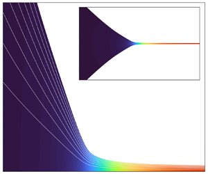
Figure 7 illustrates the importance of self-heating in the cone jet of a liquid with a high electrical conductivity such as EMI-Im. The dimensionless flow rate in this calculation has a value of 400, which is slightly smaller than the minimum flow rate reported by Gamero-Castaño & Cisquella-Serra (Reference Gamero-Castaño and Cisquella-Serra2021). The dielectric constant of EMI-Im is 12.8. Figures 7(a) and 7(b) show profiles of the currents and of the dissipation linear densities computed with both the present model and ignoring self-heating (i.e. isothermal model, we assume a constant temperature). The total current obtained with the isothermal model is 131.0 nA. When considering self-heating, the current is 62.4 % higher, 212.7 nA. Furthermore, the latter compares well with the value of 203 nA for  $\varPi _Q = 400$ from the fitting of experimental data reported by Gamero-Castaño & Cisquella-Serra (Reference Gamero-Castaño and Cisquella-Serra2021). When self-heating is accounted for, the ohmic and viscous dissipations are respectively much larger and much smaller than in the isothermal calculation. This is an obvious effect of the temperature increase along the cone jet and the associated enhancement of the electrical conductivity and the reduction of the viscosity, together with the proportionality between ohmic dissipation and electrical conductivity, (3.5), and between viscous dissipation and viscosity, (3.8). Figure 7(c) shows the variation of the temperature, electrical conductivity and viscosity along the axis computed with the present model, and the ratio $R/R_0$ between the radii of the surfaces for the present and the isothermal models. The total temperature increase along this section of the cone jet is 93.3 $\,^\circ$C, the electrical conductivity increases by a factor of 5.7 and the viscosity is reduced by a factor of 7.6. The very significant changes in these two key physical properties show that an isothermal description of these cone jets would be grossly incorrect. The strong variation of the electrical conductivity and the scaling law (1.1) readily explain the enhanced value of the total current with respect to the isothermal solution, 212.7 nA vs 131.0 nA. The ratio $R/R_0$ is 1 upstream, increases up to a maximum value of 1.087 at $x-x_0=45.6$ and decreases downstream to a value of 0.9. The larger current and the smaller jet radius in the presence of self-heating follow the electrical conductivity trend in the scaling laws (1.1) and (1.2). The dependencies are quantitatively weaker, but this is to be expected from the gradual increase of the electrical conductivity along the transition region. Finally, the contour plot in figure 7(d) shows the lack of radial variation of the temperature in the slender jet. Although not explored in this paper, the ability to compute the temperature field along the cone jet is key to study ion-field evaporation, an emission mechanism that strongly depends on temperature and that plays a main role in the electrosprays of highly conducting liquids, including EMI-Im (Gamero-Castaño & Cisquella-Serra Reference Gamero-Castaño and Cisquella-Serra2021).

Figure 7. Numerical solution for EMI-Im,  $\varPi _Q=400$, $Re=8.51\times 10^{-3}$, $Pe=13.6$, $\varepsilon =12.8$. The red curves correspond to the isothermal solution while the blue curves consider self-heating: (a) bulk and surface current; (b) ohmic and viscous dissipation linear density; (c) temperature increase, electrical conductivity and viscosity along the axis for the self-heating case, and the ratio between the radii of the surfaces for the self-heating ( $R$) and isothermal ( $R_0$) cases; (d) 2-D map of the temperature increase in the cone jet (self-heating case).
The significant increase of temperature in liquids with high electrical conductivity explains their abnormal current versus flow rate behaviour. Figure 8 compares experimental values (Gamero-Castaño Reference Gamero-Castaño2019) with the numerical solution, for electrosprays of propylene carbonate and ethylene glycol with several electrical conductivities (or, equivalently, Reynolds numbers). The experimental data for each conductivity exhibits the well-known  $\tilde {I} \propto \tilde {Q}^{1/2}$ law. When plotted in dimensionless form, $\tilde {I} / \sqrt {\varepsilon _0\gamma ^2/\rho }$ vs $\varPi _Q$, all points for a given liquid are expected to lie on a single straight line regardless of the electrical conductivity. Although the solutions with the largest Reynolds numbers behave as expected, the data for the smaller Reynolds numbers have a vertical offset that increases with decreasing $Re$. Gamero-Castaño (Reference Gamero-Castaño2019) explained this anomaly as an effect of energy dissipation and the consequent self-heating of the liquid, expected to increase at decreasing $Re$: when the temperature in the transition region increases significantly, using the emitter temperature to evaluate $\varPi _Q$ underestimates its value, shifting leftward the experimental data ( $\varPi _Q$ is proportional to the electrical conductivity, which increases with temperature). The numerical results in figure 8 confirm this explanation. The numerical solution matches well the experimental data, reproducing the vertical offset of the current versus flow rate curves at low $Re$. The vertical offset starts to be significant at a Reynolds number of approximately 0.3, for which the computed temperature increase is approximately 2 $\,^\circ$C. The liquid solutions used in the experiments were obtained by adding increasing quantities of EMI-Im to propylene carbonate and ethylene glycol, in order to increase the electrical conductivity. The uncertainty in the values of the physical properties of these mixtures, which increases at decreasing $Re$, are likely responsible for the differences between numerical and experimental results. Note that the comparison between the numerical solution and the experimental value in the case of EMI-Im is excellent, 212.7 nA vs 203 nA for $\varPi _Q = 400$, even though self-heating is significantly more intense in EMI-Im than in any state shown in figure 8. Unlike the propylene carbonate and ethylene glycol solutions, EMI-Im is a pure liquid with accurate $K(T)$ and $\mu (T)$ functions (Kazakov et al. Reference Kazakov, Magee, Chirico, Paulechka, Diky, Muzny, Kroenlein and Frenkel2022).

Figure 8. Current versus flow rate, comparison between measurements (solid circles) and model results (open squares and triangles) for ethylene glycol solutions (a) and propylene carbonate solutions (b).
4. Conclusions
Ohmic and viscous dissipations in cone jets increase the temperature of the liquid, linking electrohydrodynamic and thermal phenomena. In this paper we self-consistently study this coupling for the first time, using an extension of the leaky-dielectric model that includes conservation of energy and temperature-dependent functions for the viscosity and the electrical conductivity. We find that the temperature increase is a function of the physical properties of the liquid and its flow rate, (3.10); for a given liquid, the maximum temperature increase only depends on the physical properties, (3.11), with the electrical conductivity playing a key role (the maximum temperature scales with  $K^{2/3}$); and temperature increases of a few centigrade degrees occur in liquids with electrical conductivities as low as 0.01 S m $^{-1}$. Therefore, when modelling cone jets or analysing experimental data, it is important to account for self-heating when the electrical conductivity is of the order or larger than 0.01 S m $^{-1}$, which includes the conductivity values needed to produce droplets and jets with diameters of tens of nanometres or smaller.
Viscous dissipation concentrates in the transition from cone to jet. The generation of ohmic dissipation starts in this region and continues in a longer section of the jet where bulk conduction current transforms into surface current. In the operational range of cone jets where self-heating is significant the ohmic term is the main contributor to the total dissipation, and only near the minimum flow rate, i.e. near the condition  $\varPi _Q = 1/Re$, ohmic and viscous dissipations are comparable. Because of the distribution of dissipation, the temperature increases in the section of the jet where charge is injected from the bulk of the liquid onto the surface. The physical properties of the liquid, especially the viscosity and the electrical conductivity, are functions of the temperature, and their values change along this section where the total current and the diameter of the jet are fixed. Therefore, the traditional scaling laws for cone jets, which assume constant values of the physical properties, become increasingly inaccurate as self-heating intensifies. An example of this effect is the unexpected vertical offset of the dimensionless current versus flow rate function observed in liquids with high electrical conductivities. This work shows that this vertical offset is an artifact of employing the traditional scaling laws in cone jets in which self-heating induces significant temperature variations.
Funding
This work was funded by the Air Force Office of Scientific Research, award no. FA9550- 21-1-0200.
Declaration of interests
The authors report no conflict of interest.
Appendix A. Regular perturbation solution for the jet region
The jet solution in region  $\varSigma _3$ is obtained by applying Poincaré's perturbation method (Paulsen Reference Paulsen2013) to the equation set (2.1)–(2.12). The quantities of interest (stream function, vorticity, electric potential and temperature) are expressed as a series using $R(x)$ as the expansion parameter:
 \begin{equation} \left.\begin{array}{c@{}} \displaystyle \varPsi=\sum_{j=0}^\infty{R^j\varPsi_j}=\varPsi_0+R\varPsi_1+R^2\varPsi_2+\cdots, \\ \displaystyle \varOmega=\sum_{j=0}^\infty{R^j\varOmega_j}=\varOmega_0+R\varOmega_1+R^2\varOmega_2+\cdots, \\ \displaystyle \varPhi_i=\sum_{j=0}^\infty{R^j\varPhi_{i,j}}=\varPhi_{i,0}+R\varPhi_{i,1}+R^2\varPhi_{i,2}+\cdots, \\ \displaystyle T=\sum_{j=0}^\infty{R^jT_j}=T_0+RT_1+R^2T_2+\cdots. \end{array}\right\}\end{equation}
Equations (2.1), (2.2), (2.4) and (2.3) are written in terms of  $\varPsi$ and $\varOmega$ and in the orthogonal coordinates $\xi$, $\eta$ (see Appendix B) as
 \begin{align} &\frac{\eta(1+\eta^2R'^2)}{R^2}\frac{\partial^2\varPsi}{\partial\eta^2}+ \frac{\eta}{{x_\xi}^2(1+\eta^2R'^2)}\frac{\partial^2\varPsi}{\partial \xi^2}+\frac{\eta^2(2R'^2-RR'')-1}{R^2}\frac{\partial\varPsi}{\partial\eta}\nonumber\\ &\quad -\left[\frac{2\eta^3R'R''}{x_\xi(1+\eta^2R'^2)^2}+ \frac{\eta x_{\xi\xi}}{{x_\xi}^3(1+\eta^2R'^2)}\right] \frac{\partial\varPsi}{\partial\xi}=-\eta^2R\varOmega, \end{align}
 \begin{align} &\frac{\eta^2(1+\eta^2{R'}^2)}{R^2}\frac{\partial^2\varOmega}{\partial\eta^2} +\frac{\eta^2}{{x_\xi}^2(1+\eta^2R'^2)} \frac{\partial^2\varOmega}{\partial\xi^2} +\frac{\eta^3(2R'^2-RR'')+\eta}{R^2}\frac{\partial\varOmega}{\partial\eta}\nonumber\\ &\qquad +\frac{\eta^2}{x_\xi(1+\eta^2R'^2)} \left[\frac{2R'}{R}-\frac{2\eta^2R'R''}{1+\eta^2R'^2}- \frac{x_{\xi\xi}}{{x_\xi}^2}\right]\frac{\partial\varOmega}{\partial\xi} -\frac{\varOmega}{R^2}\nonumber\\ &\quad =\frac{\mu_0Re\sqrt{\varPi_Q}}{{\rm \pi}\mu R^2} \left[\frac{\eta}{x_\xi}\left(\frac{\partial\varPsi}{\partial\eta} \frac{\partial\varOmega}{\partial\xi}-\frac{\partial\varPsi}{\partial\xi} \frac{\partial\varOmega}{\partial\eta}\right)+ \left(\frac{1}{x_\xi(1+\eta^2{R'}^2)} \frac{\partial\varPsi}{\partial\xi}-\frac{\eta R'}{R} \frac{\partial\varPsi}{\partial\eta}\right)\varOmega\right]\nonumber\\ &\qquad -\frac{1}{\mu\eta R}\left[\left(\frac{\partial^2\varPsi}{\partial x^2}- \frac{\partial^2\varPsi}{\partial r^2}+\frac{1}{\eta R} \frac{\partial\varPsi}{\partial r}\right)\left(\frac{\partial^2\mu}{\partial r^2}- \frac{\partial^2\mu}{\partial x^2}\right)+\left(\frac{2}{\eta R} \frac{\partial\varPsi}{\partial x}-4\frac{\partial^2\varPsi}{\partial x\partial r}\right)\frac{\partial^2\mu}{\partial x\partial r}\right.\nonumber\\ &\qquad +\left.\frac{\partial\varOmega}{\partial x} \frac{\partial\mu}{\partial x}+\frac{\partial\varOmega}{\partial r} \frac{\partial\mu}{\partial r}\right]\!, \end{align}
 \begin{align} &\frac{1{\,+\,}\eta^2R'^2}{R^2}\frac{\partial^2\varPhi_i}{\partial\eta^2}{\,+\,} \frac{1}{{x_\xi}^2(1{\,+\,}\eta^2R'^2)}\frac{\partial^2\varPhi_i}{\partial\xi^2}{\,+\,} \left[\frac{1}{\eta}{\,+\,}\eta(2R'^2{\,-\,}RR''){\,+\,}\frac{1{\,+\,}\eta^2R'^2}{K} \frac{\partial K}{\partial\eta}\right] \frac{1}{R^2}\frac{\partial\varPhi_i}{\partial\eta}\nonumber\\ &\quad {\,+\,}\frac{1}{x_\xi(1{\,+\,}\eta^2R'^2)}\left[\frac{2R'}{R}{\,-\,} \frac{2\eta^2R'R''}{1{\,+\,}\eta^2R'^2}-\frac{x_{\xi\xi}}{{x_\xi}^2}+ \frac{1}{x_\xi K}\frac{\partial K}{\partial\xi}\right] \frac{\partial\varPhi_i}{\partial\xi}=0, \end{align}
 \begin{align} &\frac{1+\eta^2R'^2}{R^2}\frac{\partial^2 T}{\partial\eta^2}+ \frac{1}{{x_\xi}^2(1+\eta^2R'^2)}\frac{\partial^2 T}{\partial\xi^2}+ \left[1+\eta^2(2R'^2-RR'')+\frac{Pe}{x_\xi}\frac{\partial\varPsi}{\partial\xi}\right] \frac{1}{\eta R^2}\frac{\partial T}{\partial\eta}\nonumber\\ &\qquad +\left[\frac{1}{1+\eta^2R'^2}\left(\frac{2R'}{R}- \frac{2\eta^2R'R''}{1+\eta^2R'^2}-\frac{x_{\xi\xi}}{{x_\xi}^2}\right)- \frac{Pe}{\eta R^2}\frac{\partial\varPsi}{\partial\eta}\right] \frac{1}{x_\xi}\frac{\partial T}{\partial\xi}\nonumber\\ &\quad=\frac{\mu Pe}{\mu_0Re\sqrt{\varPi_Q}\eta^2R^2} \left[2\frac{\partial^2\varPsi}{\partial x\partial r}^2+ \left(\frac{\partial^2\varPsi}{\partial r^2}-\frac{\partial^2\varPsi}{\partial x^2}- \frac{1}{\eta R}\frac{\partial\varPsi}{\partial r}\right)^2\right.\nonumber\\ &\qquad+2 \left.\left(\frac{1}{\eta R}\frac{\partial\varPsi}{\partial x}- \frac{\partial^2\varPsi}{\partial x\partial r}\right)^2+ \frac{2}{\eta^2R^2}\frac{\partial\varPsi}{\partial x}^2\right]\nonumber\\ &\qquad +\frac{K Pe}{K_0\sqrt{\varPi_Q}}\left(\frac{1}{{x_\xi}^2 (1+\eta^2R'^2)}\frac{\partial\varPhi_i}{\partial\xi}^2+ \frac{1+\eta^2R'^2}{R^2}\frac{\partial\varPhi_i}{\partial\eta}^2\right)\!. \end{align}
To apply the perturbation method, we first identify all the terms in these equations that are small in the jet region. Downstream of the liquid surface is slender ( $R'\ll 1$, $R''\ll 1$) and the fluid velocity is well aligned with the axial coordinate ( $v_\eta \propto {\partial \varPsi }/{\partial \xi }\ll 1$). Also, since $\xi$ and $x$ are nearly parallel, $R$,
$R$,  $R'$,
$R'$,  $R''$ are considered a function of $\xi$ only. These observations are summarized as the jet hypotheses:
 \begin{equation} \left.\begin{array}{c@{}} \displaystyle R'^2\cong 0, \quad \dfrac{\partial\varPsi}{\partial\xi}\cong 0, \quad \dfrac{\partial^2\varPsi}{\partial\xi^2}\cong 0,\\ R\cong R(\xi), \quad R'\cong R'(\xi), \quad R''\cong R''(\xi),\\ x_\xi\cong x_\xi(\xi), \quad x_{\xi\xi}\cong x_{\xi\xi}(\xi). \end{array}\right\}\end{equation}
By applying (A6) to (A2)–(A5) we eliminate all the higher-order terms and obtain
 $$\begin{gather} \eta\frac{\partial^2\varPsi}{\partial\eta^2}+[\eta^2(2R'^2-RR'')-1] \frac{\partial\varPsi}{\partial\eta}=-\eta^2R^3\varOmega, \end{gather}$$
 $$\begin{gather}\eta^2\frac{\partial^2\varOmega}{\partial\eta^2}- \frac{\mu_0Re\sqrt{\varPi_Q}}{{\rm \pi}\mu}\frac{\partial\varPsi}{\partial\eta} \frac{\eta}{x_\xi}\frac{\partial\varOmega}{\partial\xi}+\eta \frac{\partial\varOmega}{\partial\eta}-\varOmega=0, \end{gather}$$
 $$\begin{gather}\frac{\partial^2\varPhi_i}{\partial\eta^2}+\left(\frac{1}{\eta}-\eta R R''\right) \frac{\partial\varPhi_i}{\partial\eta}+\frac{2RR'}{x_\xi} \frac{\partial\varPhi_i}{\partial\xi}=0, \end{gather}$$
 $$\begin{gather}\frac{\partial^2T}{\partial\eta^2}+\frac{1}{\eta}\frac{\partial T}{\partial\eta}- \frac{Pe}{x_\xi}\frac{\partial T}{\partial\xi}=-\frac{12Pe\mu}{\mu_0 Re\sqrt{\varPi_Q}}\frac{R'^2}{R^4}-\frac{Pe K}{K_0\sqrt{\varPi_Q}} (R E_t)^2. \end{gather}$$
These equations are still too complex to be solved analytically. In order to obtain a solution we substitute  $\varPsi$, $\varOmega$, $\varPhi _i$ and $T$ for their expansions (A1), and separate terms according to their order $R^i$.
For the vorticity, we obtain the equation
 \begin{equation} \eta^2\frac{\partial^2\varOmega_0}{\partial\eta^2}+\eta \frac{\partial\varOmega_0}{\partial\eta}-\varOmega_0=0\end{equation}
for the zeroth-order term. Higher-order terms are still too complex to be solved analytically. The solution of (A11), using (2.9) and the symmetry condition  $\varOmega (x,0)=0$ as boundary conditions, is
 \begin{equation} \varOmega_0=\frac{2R''}{R^2(1+R'^2)} \left.\frac{\partial\varPsi}{\partial\eta}\right|_{\eta=1}- \frac{\mu_0Re}{2\mu}E_t\sigma.\end{equation}
We apply the vorticity solution (A12)–(A7), to obtain the following equation set for the stream function:
 \begin{align} \left.\begin{array}{c@{}} \displaystyle \eta\dfrac{\partial^2\varPsi_0}{\partial\eta^2}- \dfrac{\partial\varPsi_0}{\partial\eta}=0,\\ \displaystyle \eta\dfrac{\partial^2\varPsi_1}{\partial\eta^2}- \dfrac{\partial\varPsi_1}{\partial\eta}=\eta^2 \left(R''-\dfrac{2R'^2}{R}\right)\dfrac{\partial\varPsi_0}{\partial\eta}- \eta^3\left(2R''\left.\dfrac{\partial\varPsi_0}{\partial\eta} \right|_{\eta=1}-\dfrac{\mu_0Re}{2\mu}R^2E_t\sigma\right). \end{array}\right\}\end{align}
In this case we solve analytically for the first two terms of the  $\varPsi$ expansion. The boundary conditions in this case are
 \begin{equation} \left.\begin{array}{c@{}} \varPsi_0(\xi,0)=0, \quad \varPsi_0(\xi,1)=1/2,\\ \varPsi_1(\xi,0)=0, \quad \varPsi_1(\xi,1)=0, \end{array}\right\}\end{equation}
where the value of  $\varPsi$ on the surface is obtained from the dimensionless flow rate. The solution of these equations is then
 \begin{equation} \left.\begin{array}{c@{}} \displaystyle \varPsi_0=\dfrac{\eta^2}{2},\\ \displaystyle \varPsi_1=\dfrac{\eta^4-\eta^2}{8}\left(\dfrac{\mu_0Re}{2\mu}R^2 E_t\sigma-R''-\dfrac{2R'^2}{R}\right)\!. \end{array}\right\}\end{equation}
For the electric potential, we apply the same procedure. Equation (A9) is expanded as
 \begin{equation} \left.\begin{array}{c@{}} \displaystyle \eta\dfrac{\partial^2\varPhi_{i,0}}{\partial\eta^2}+ \dfrac{\partial\varPhi_{i,0}}{\partial\eta}=0,\\ \displaystyle \dfrac{\partial^2\varPhi_{i,1}}{\partial\eta^2}+ \dfrac{1}{\eta}\dfrac{\partial\varPhi_{i,1}}{\partial\eta}=\eta R'' \dfrac{\partial\varPhi_{i,0}}{\partial\eta}-\dfrac{2R'}{x_\xi} \dfrac{\partial\varPhi_{i,0}}{\partial\xi}=2R' E_t, \end{array}\right\}\end{equation}
with boundary conditions
 \begin{equation} \left.\begin{array}{c@{}} \varPhi_{i,0}(\xi,0)=0, \quad \varPhi_{i,0}(\xi,1)=\varPhi_s,\\ \varPhi_{i,1}(\xi,0)=0, \quad \varPhi_{i,1}(\xi,1)=0. \end{array}\right\}\end{equation}
The final result is
 \begin{equation} \left.\begin{array}{c@{}} \varPhi_{i,0}=\varPhi_s,\\ \varPhi_{i,1}=\dfrac{RR'(\eta^2-1)}{2}E_t. \end{array}\right\}\end{equation}
 Obtaining a solution for the jet temperature is more complicated. In this case the  ${\partial }/{\partial \xi }$ term cannot be eliminated from the zeroth-order equation, but the differential equation can be solved using separation of variables. Since in this case we only solve for $T_0$, we use $T$ in the equations for simplicity. The temperature is assumed to be of the form
 \begin{equation} T(\xi,\eta)=f(\xi)+g(\xi)h(\eta). \end{equation}
Leading to the equation
 \begin{equation} \frac{1}{x_\xi}\frac{{\rm d} f}{{\rm d} \xi}+\frac{h}{x_\xi} \frac{{\rm d} g}{{\rm d} \xi}-\frac{g}{Pe}\left(\frac{1}{\eta} \frac{{\rm d} h}{{\rm d} \eta}+\frac{{\rm d}^2h}{{\rm d} \eta^2}\right)= \frac{1}{\sqrt{\varPi_Q}}\left[\frac{12\mu R'^2}{\mu_0Re R^4}+ \frac{K}{K_0}(R E_t)^2\right]\!.\end{equation}
The solution for  $f$,
$f$,  $g$ and $h$ is then
 \begin{equation} \left.\begin{array}{c@{}} \displaystyle f(\xi)=f_0+\dfrac{1}{\sqrt{\varPi_Q}}\int_{x_{23}}^{x} \left[\dfrac{12\mu R'^2}{\mu_0Re R^4}+\dfrac{K}{K_0}(R E_t)^2\right]\,{{\rm d} x},\\ \displaystyle g(\xi)=g_0\exp\left[-\dfrac{C^2}{Pe}(x-x_{23})\right]\!,\\ h(\eta)=h_0J_0(C\eta)+h_1Y_0(C\eta), \end{array}\right\}\end{equation}
where  $J_0()$ and $Y_0()$ are the Bessel functions of order zero of the first and second kind and $C$ is a constant to be found. As boundary conditions, we have
 \begin{equation} \frac{\partial T}{\partial\eta}(\xi,0)=0, \quad \frac{\partial T}{\partial\eta}(\xi,1)=0.\end{equation}
From these conditions we obtain  $h_0=1$, $h_1=0$ and $C=j_{1,n}\varepsilon ^{1/2}$, where $j_{1,n}$ is the $n$th zero of the Bessel functions of the first kind of order one. These definitions result in
 \begin{align}
T_{jet} &=f_0+\frac{1}{\sqrt{\varPi_Q}}\int_{x_{23}}^x{\left(\frac{12\mu}{\mu_0Re}
\frac{R'^2}{R^4}+\frac{K}{K_0}R^2{E_t}^2\right)}\, {{\rm d}
x}\notag\\ &\quad +\sum_{n=1}^\infty{g_nJ_0(\eta
j_{1,n})\exp\left[-\frac{{j_{1,n}}^2}{Pe}(x-x_{23})\right]}.\end{align}
\begin{align}
T_{jet} &=f_0+\frac{1}{\sqrt{\varPi_Q}}\int_{x_{23}}^x{\left(\frac{12\mu}{\mu_0Re}
\frac{R'^2}{R^4}+\frac{K}{K_0}R^2{E_t}^2\right)}\, {{\rm d}
x}\notag\\ &\quad +\sum_{n=1}^\infty{g_nJ_0(\eta
j_{1,n})\exp\left[-\frac{{j_{1,n}}^2}{Pe}(x-x_{23})\right]}.\end{align}
Finally, the constants  $f_0$ and $g_n$ are obtained by matching the temperature and its derivative at the base of the jet ( $x=x_{23}$):
 \begin{equation} \left.\begin{array}{c@{}} \displaystyle f_0=2\int_0^1{\eta T(x_{23},\eta)}\, {\rm d} \eta,\\ \displaystyle g_n=\dfrac{2}{{J_0(\,j_{1,n})}^2}\int_0^1{\eta J_0(\eta j_{1,n})\left(T(x_{23},\eta)-f_0\right)}\, {\rm d} \eta. \end{array}\right\}\end{equation}
Appendix B. Coordinate system orthogonal to the surface of the cone jet
In region  $\varSigma _2$ the equation set is solved using finite differences in an orthogonal grid with coordinates $\xi$, $\eta$ (see figure 9). Region $\varSigma _2$ is bounded by the symmetry axis and by the liquid surface, allowing us to define an orthogonal frame of reference using a variation of the method given by Srinivas & Fletcher (Reference Srinivas and Fletcher2002). Starting from equation
 \begin{equation} \frac{{\rm d} \xi}{{\rm d} \eta}=-\frac{\dfrac{\partial x}{\partial\xi}\dfrac{\partial x}{\partial\eta}+\dfrac{\partial r}{\partial\xi}\dfrac{\partial r}{\partial\eta}}{\dfrac{\partial x}{\partial\xi}^2+\dfrac{\partial r}{\partial\eta}^2}, \end{equation}
we first redefine  $x,r$ as
 \begin{equation} \left.\begin{array}{c@{}} x=x(\xi,\eta),\\ r=\eta R(x), \end{array}\right\}\end{equation}
where  $\xi$ and $\eta$ are the two orthogonal variables, and $x()$ is a generic function of $\xi,\eta$. The coordinate $\eta$ is equal to 0 at the symmetry axis and 1 at the surface, while $\xi$ goes from 0 on the upstream boundary $x_{12}$ to 1 at the downstream boundary $x_{23}$. By applying (B2) into (B1), we obtain
 \begin{equation} \frac{{\rm d} \xi}{{\rm d} \eta}=-x_\xi\frac{x_\eta+\eta R R'+\eta^2x_\eta {R'}^2}{{x_\xi}^2(R+\eta x_\eta R')^2}. \end{equation}
We enforce the orthogonality of the  $\xi,\eta$ coordinates by requiring $\textrm {d}\xi /\textrm {d}\eta =0$. This leads to
 \begin{equation} \frac{\partial x}{\partial\eta}=\frac{-\eta R R'}{1+\eta^2{R'}^2}. \end{equation}
This equation is integrated from  $\eta =1$ to $\eta =0$, using the initial condition the distribution of points on the surface $R(x)$, to obtain the $x$ coordinate of all the points in the orthogonal grid. To obtain the $r$ coordinate, we use the definition of $r$ in (B2) together with the computed $x$ coordinates.

Figure 9. Example of the orthogonal grid defined in region  $\varSigma _2$. The inset zooms on the base of the jet.
All the equations used in the model are converted from  $x$,
$x$,  $r$ to $\xi$, $\eta$ coordinates by using
 $$\begin{align} \frac{\partial}{\partial x}&=\frac{1}{x_\xi(1+\eta^2{R'}^2)}\frac{\partial}{\partial\xi}-\frac{\eta R'}{R}\frac{\partial}{\partial\eta}, \end{align}$$
 $$\begin{align}\frac{\partial}{\partial r}&=\frac{\eta R'}{x_\xi(1+\eta^2{R'}^2)}\frac{\partial}{\partial\xi}+ \frac{1}{R}\frac{\partial}{\partial\eta}, \end{align}$$
 \begin{align} \frac{\partial^2}{\partial x^2}&=\frac{1}{[x_\xi(1+\eta^2R'^2)]^2} \frac{\partial^2}{\partial\xi^2}+\left(\frac{\eta R'}{R}\right)^2 \frac{\partial^2}{\partial\eta^2}-\frac{2\eta R'}{Rx_\xi(1+\eta^2R'^2)} \frac{\partial^2}{\partial\xi\partial\eta}\nonumber\\ &\quad +\frac{1}{x_\xi(1+\eta^2R'^2)^2}\left[\eta^2R' \left(\frac{R'^2-RR''}{R}-\frac{2R''}{1+\eta^2R'^2}\right)- \frac{x_{\xi\xi}}{{x_\xi}^2}\right]\frac{\partial}{\partial\xi}\notag\\ &\quad +\frac{\eta(2R'^2-RR'')}{R^2}\frac{\partial}{\partial\eta}, \end{align}
 \begin{align} \frac{\partial^2}{\partial r^2}&=\frac{\eta^2R'^2}{[x_\xi(1+\eta^2R'^2)]^2} \frac{\partial^2}{\partial\xi^2}+\frac{1}{R^2}\frac{\partial^2}{\partial\eta^2}+ \frac{2\eta R'}{Rx_\xi(1+\eta^2R'^2)}\frac{\partial^2}{\partial\xi\partial\eta}\nonumber\\ &\quad +\frac{R'}{x_\xi(1+\eta^2R'^2)^2}\left[\frac{1}{R}+\eta^2R'' \frac{1-\eta^2R'^2}{1+\eta^2R'^2}-\frac{\eta R' x_{\xi\xi}}{{x_\xi}^2}\right] \frac{\partial}{\partial\xi}, \end{align}
 \begin{align} \frac{\partial^2}{\partial x\partial r}&= \frac{\eta R'}{[x_\xi(1+\eta^2R'^2)]^2}\frac{\partial^2}{\partial\xi^2}- \frac{\eta R'}{R^2}\frac{\partial^2}{\partial\eta^2}+ \frac{1-\eta^2R'^2}{Rx_\xi(1+\eta^2R'^2)} \frac{\partial^2}{\partial\xi\partial\eta}\nonumber\\ &\quad +\frac{\eta}{x_\xi(1+\eta^2R'^2)^2}\left[R''\frac{1-\eta^2R'^2}{1+ \eta^2R'^2}-\frac{R'^2}{R}-\frac{R' x_{\xi\xi}}{{x_\xi}^2}\right] \frac{\partial}{\partial\xi}-\frac{R'}{R^2}\frac{\partial}{\partial\xi}, \end{align}


 Open access