


1. Introduction
Binary droplet collisions have been a research topic for more than a century and continue to be an active research topic due to their complexity and many applications. In its simplest form, the problem consists of two liquid droplets approaching each other at a constant velocity, headed for a collision. Typically, these droplets are immersed in a fluid, such as air, with a smaller viscosity than the droplets – for example, aerosol fuel droplets merging or splashing in combustion chambers (Jiang, Umemura & Law Reference Jiang, Umemura and Law1992; Chen Reference Chen2007) in which the ignition and propagation of the flames depend on the atomisation of the fuel (Ozel-Erol et al. Reference Ozel-Erol, Hasslberger, Klein and Chakraborty2018). Another example concerns the drying of suspensions such as milk (Finotello et al. Reference Finotello, Kooiman, Padding, Buist, Jongsma, Innings and Kuipers2017), paint pigments or pharmaceutical powders (Mujumdar Reference Mujumdar2014). In these applications, large droplets may not dry out completely; on the contrary, if the droplets are too small, undesirable dust particles are produced. The main objective in the study of binary droplet collisions can be summarised as predicting the outcome of the collision for a given set of initial conditions (Ashgriz & Poo Reference Ashgriz and Poo1990). In other words, identifying the conditions under which the droplets coalesce, bounce or splash, disintegrating into several small droplets after the collision, remains important. Early studies in binary droplet collisions can be dated back to Rayleigh (Reference Rayleigh1945), who reported that droplets may coalesce and break up into several smaller droplets or bounce apart after a collision. Most of the early experiments were conducted for water droplets (Adam, Lindblad & Hendricks Reference Adam, Lindblad and Hendricks1968; Brazier-Smith et al. Reference Brazier-Smith, Jennings, Latham and Mason1972) primarily to model atmospheric phenomena such as cloud formation. Those experiments suggest that the three main parameters that determine the outcome of the collision are the Weber number  $We := \rho (d_1 + d_2) u_r^2 / 2 \sigma$ and the impact parameter $B := 2 b / (d_1 + d_2)$, where $\rho$ is the density of the liquids, $d_i$
$d_i$  $(i = 1, 2)$ is the diameter of the droplets, $\sigma$ is the surface tension, $b$ is the separation distance between the centres of mass of the droplets and $u_r$ is the magnitude of the relative velocity. The Weber number quantifies the relative kinetic energy in proportion to the interfacial energy, and the impact parameter is a measure of the off-centredness of the collision. It was found that for small $We$ and $B$, the droplets undergo a slow coalescence; increasing either $We$ or $B$ results in the bouncing of the droplets due a layer of air trapped between the droplets. Coalescence is recovered by further increasing the relative velocity of the droplets (Orme Reference Orme1997; Qian & Law Reference Qian and Law1997); however, a head-on separation or fragmentation may follow, depending on the impact parameter. This is usually summarised by a phase diagram in the $We$–
$We$– $B$ space, also known as the collision map, which indicates the different outcomes that are expected for a given pair of $We$ and $B$ (Al-Dirawi & Bayly Reference Al-Dirawi and Bayly2019). However, the collision map is not unique and other parameters, such as the viscosity of the liquids and surrounding phase and its pressure, also determine the outcome of the collision (Chesters Reference Chesters1991). For example, Willis & Orme (Reference Willis and Orme2000) conducted experiments in a vacuum chamber, thus revealing the effect of the outer phase. Further experimental studies have focused on the interaction of non-Newtonian (Finotello et al. Reference Finotello, De, Vrouwenvelder, Padding, Buist, Jongsma, Innings and Kuipers2018) or immiscible liquids (Planchette, Lorenceau & Brenn Reference Planchette, Lorenceau and Brenn2010).
Theoretical and numerical studies have also addressed the main problem of the collision of binary droplets. Gopinath & Koch (Reference Gopinath and Koch2002) devised a model for a head-on collision identifying the boundaries between the regions in the collision map. Later, Roisman (Reference Roisman2004, Reference Roisman2009) proposed a model giving an approximation of the flow field at early stages of a head-on collision and successfully predicted the thickness of the liquid lamella and the outer rim that is formed after coalescence. In the meantime, lattice Boltzmann (Inamuro, Tajima & Ogino Reference Inamuro, Tajima and Ogino2004) and level-set (Pan & Kazuhiko Reference Pan and Kazuhiko2005) simulations were being developed. Kuan, Pan & Shyy (Reference Kuan, Pan and Shyy2014) conducted a detailed study of droplet splashing using the interface-tracking method combined with adaptive mesh refinement. The applications that are based on the precise outcome of the collision of droplets are technologies that include drop-on-demand manufacturing such as bioprinting processes. The reactive jet impingement (ReJI) technology (da Conceicao Ribeiro et al. Reference da Conceicao Ribeiro, Pal, Ferreira, Gentile, Benning and Dalgarno2018), for example, consists of a stream of cell-laden droplets of a gel precursor and a cross-linker that are injected and collide in mid-air to then mix and react to build the designed living tissue. This novel technique for bioprinting shows a significant improvement over other techniques in terms of cell viability and printing speed. In ReJI, as well as several adaptive manufacturing techniques, the quality of the product and throughput depends on the speed of injection and size of the droplets (Stringer & Derby Reference Stringer and Derby2009). This imposes a limit on the Weber number for droplet stacking (Son et al. Reference Son, Kim, Yang and Ahn2008) and mid-air collisions (Barker et al. Reference Barker, Lewns, Poologasundarampillai and Ward2022). Furthermore, the complexity in the modelling of additive manufacturing processes increases from the idealised droplet collision. For example, when colliding, the morphology of the droplets does not relax to a spherical shape, requiring a redefinition of the impact parameter.
Another key aspect in the quality of printing technologies concerns the mixing of the inks as the droplets collide in mid-air. Although mixing is present in our everyday lives, quantifying mixing (Rasband Reference Rasband1990; Cornfeld et al. Reference Cornfeld, Sossinskii, Fomin and Sinai2012) and controlling and optimising the mechanisms that affect it remain complex (Lin, Thiffeault & Doering Reference Lin, Thiffeault and Doering2011; Lunasin et al. Reference Lunasin, Lin, Novikov, Mazzucato and Doering2012). Intuitively, one can acknowledge a state where two substances are completely mixed if the resulting material becomes homogeneous in appearance, therefore, when the gradients of the concentration of the two substances vanish (Aref Reference Aref1984; Rom-Kedar, Leonard & Wiggins Reference Rom-Kedar, Leonard and Wiggins1990; Walters Reference Walters2000). Mixing can also be partial (Thiffeault Reference Thiffeault2012), which would correspond to an intermediate state in which, by some transformation, such as stirring, the components of the systems are transformed from a heterogeneous state into a homogeneous one (Foures, Caulfield & Schmid Reference Foures, Caulfield and Schmid2014). When the motion of the fluid is accompanied by diffusion, mixing becomes an irreversible process. In such cases, one can express the degree of mixing in terms of a passive scalar function (Mathew et al. Reference Mathew, Mezić, Grivopoulos, Vaidya and Petzold2007). The mixing process in the context of binary droplet collisions has been addressed before; this includes the work by Anilkumar, Lee & Wang (Reference Anilkumar, Lee and Wang1991), who investigated experimentally the quiescent coalescence of drops of the same liquid. Liu et al. (Reference Liu, Zhang, Law and Guo2013), limiting their study to axisymmetric collisions of spherical droplets, used a front tracking algorithm combined with a set of Lagrangian particles to monitor the distribution of liquids. Later, Sun et al. (Reference Sun, Zhang, Law and Wang2015) studied a similar set-up and proposed a way of quantifying partial mixing of non-Newtonian droplets.
In this work, the mixing process resulting from a binary droplet collision of non-spherical droplets is studied. This includes identifying the conditions that result in the most efficient mixing. Most bioprinting techniques employ materials of a wide variety of properties, e.g. rheology and surface tension. However, to aid the development of such technologies, the present work is focused on understanding the mechanisms emerging from the collision of droplets with identical properties. In § 2, the underlying physical mechanisms that govern mixing in a binary droplet collision are discussed. Then, in § 3, the numerical methods and the tools for analysing the results are described, and the results are presented in § 4. Finally, conclusions are summarised in § 5.
2. Governing equations
The fluid components are modelled by three concentration fields  $\alpha _i(\boldsymbol {x}) \in [0, 1]$, $i = 1, 2, 3$, where $\alpha _1$ and $\alpha _2$ correspond to liquids L1 and L2, respectively, $\alpha _3$ corresponds to the surrounding gas phase and $\boldsymbol {x}$ is the position vector. Here, $\alpha _i = 1$ implies the presence of component $i$, whereas $\alpha _i = 0$ implies its absence. Additionally, the constraint
 \begin{equation} \alpha_1 + \alpha_2 + \alpha_3 = 1 \end{equation}
is imposed throughout the volume of the fluid mixture  $\varOmega$. The region of the liquid is denoted by $\varOmega _l \subseteq \varOmega$, that is, $\varOmega _l = \{ \boldsymbol {x} : \alpha _1(\boldsymbol {x}) + \alpha _2(\boldsymbol {x}) = 1 \}$.
The concentration fields,  $\alpha _i$, follow the transport equation,
 \begin{equation} \partial_t \alpha_i + \boldsymbol{\nabla} \boldsymbol{\cdot} (\alpha_i \boldsymbol{u}) = \boldsymbol{\nabla} \boldsymbol{\cdot} ( D\,\boldsymbol{\nabla} \alpha_i ), \quad \boldsymbol{x} \in \varOmega_l, \end{equation}
for the liquid components  $i = 1, 2$, and
 \begin{equation} \partial_t \alpha_3 + \boldsymbol{\nabla} \boldsymbol{\cdot} (\alpha_3 \boldsymbol{u}) = 0 \end{equation}
for the gas. In this way, the two liquid components are miscible, but the liquid and gas phases are immiscible. Here,  $D$ is the diffusion coefficient and $\boldsymbol {u}$ is the velocity field that satisfies the Navier–Stokes equations,
 \begin{equation} \rho (\partial_t + \boldsymbol{u} \boldsymbol{\cdot} \boldsymbol{\nabla}) \boldsymbol{u} ={-} \boldsymbol{\nabla} p + \boldsymbol{\nabla} \boldsymbol{\cdot} (2 \rho \nu {\boldsymbol{\mathsf{S}}}) + \sigma \kappa \hat{\boldsymbol{n}}_{lg}\delta_S, \end{equation}
in the incompressible limit ( $\boldsymbol {\nabla } \boldsymbol {\cdot } \boldsymbol {u} = 0$). Here, $\rho := \sum _i \rho _i \alpha _i$ is the density of the fluid, and $\nu := \sum _i \nu _i \alpha _i$ corresponds to the kinematic viscosity, where the constants $\rho _i$ and $\nu _i$ correspond to the bulk density and viscosity of the component $i$. Also, $p$ is the pressure, ${\boldsymbol{\mathsf{S}}} := (\boldsymbol {\nabla } \boldsymbol {u} + \boldsymbol {\nabla } \boldsymbol {u}^{\rm T}) / 2$ is the strain-rate tensor, $\sigma$ is the surface tension of the liquid–gas interface, $\kappa := -\boldsymbol {\nabla } \boldsymbol {\cdot } \hat {\boldsymbol {n}}_{lg}$ is its mean curvature, $\hat {\boldsymbol {n}}_{lg}$ is the orthogonal unitary vector to the surface and $\delta _S$ represents a Dirac delta function that locates the liquid–gas interface in the three-dimensional space.
Two types of boundary conditions are imposed: these are the inlets, from which the droplets are injected, and open boundaries that allow the free movement of the flow in or out of the simulation domain specified everywhere else. As illustrated in figure 1(a), the inlets are specified at  $z = 0$ as two nozzles (indicated with subscript $nzl$ in the following) of circular cross-section of radius $R_{nzl}$ directed into the domain at the polar and azimuth angles $\theta$ and $\varphi$, respectively. More formally, to specify the region of the inlets and the open boundaries, let us define the auxiliary function
 \begin{align} G(\boldsymbol{x}; x_{nzl}, \theta, \varphi) &:= 1 - \frac{1}{R_{nzl}^2}\,\{ [(x - x_{nzl}) \cos\varphi + y \sin\varphi]^2 \cos^2 \theta \nonumber\\ &\quad + [y \cos\varphi - (x - x_{nzl}) \sin \varphi]^2\}, \end{align}
at the plane  $z = 0$. In this way, the inlets are defined as the region where $G \geq 0$. The parameter $x_{nzl}$ corresponds to the location of the centre of the inlet from the origin.

Figure 1. Simulation set-up of the binary droplet collision. (a) Schematic representation of the inlet configuration. (b) The simulation domain is a cube meshed with hexahedral cells with an increasing level of refinement closer to the path drawn by the droplets.
Each droplet is injected into the domain by a pulse of the form
 \begin{equation} T(t) := \begin{cases} 1 - \tanh[8 \cos(\omega t)] & \text{for } 0 \le t \le 2 {\rm \pi}/ \omega = T_{pulse}, \\ 0 & \text{otherwise}, \end{cases} \end{equation}
which models the timing and duration of the pulse that injects the liquids into the simulation domain, and emulates the smooth opening and closing of a typical micro-valve used for bioprinting. The orientation of the inflow is specified by the unitary vector
 \begin{equation} \hat{\boldsymbol{J}}(\theta, \varphi) := \hat{\boldsymbol{e}}_x \cos\varphi \sin\theta + \hat{\boldsymbol{e}}_y \sin\varphi \sin\theta + \hat{\boldsymbol{e}}_z \cos\theta. \end{equation}
The velocity profile at the inlets is modelled by a parabolic profile, with average velocity  $U_{nzl} := (\mathrm {d} V / \mathrm {d}t) / {\rm \pi}R_{nzl}^2$. This assumption is justified by considering that the typical Reynolds number on a bioprinting micro-valve is small ( $Re < 500$) and the nozzles of the micro-valves are long ( $\sim 20 R_{nzl}$), thus the flow field relaxes to the Poiseuille profile as opposed to a plug or a turbulent flow (da Conceicao Ribeiro et al. Reference da Conceicao Ribeiro, Pal, Ferreira, Gentile, Benning and Dalgarno2018). By combining (2.5)–(2.7), we prescribe the boundary condition for the flow field at the inlets, that is,
 \begin{equation} \boldsymbol{u}(\boldsymbol{x}, t) = \begin{cases} \begin{aligned} & (U_{nzl} + {\rm \Delta} U_{nzl})\,T(t - {\rm \Delta} t_0)\,G(\boldsymbol{x}; -x_{nzl}, \theta + {\rm \Delta} \theta, \varphi + {\rm \Delta} \varphi)\, \\[-2pt] & \quad\times \hat{\boldsymbol{J}}(\theta + {\rm \Delta} \theta, \varphi + {\rm \Delta} \varphi) \end{aligned} & \text{for L1}, \\[2pt] U_{nzl}\,T(t)\,G(\boldsymbol{x}; +x_{nzl}, \theta, \varphi) \, \hat{\boldsymbol{J}}(\theta, \varphi) & \text{for L2}, \end{cases} \end{equation}
where, without loss of generality, the new parameters introduce asymmetry between the nozzles:  ${\rm \Delta} U_{nzl}$ corresponds to a velocity difference, ${\rm \Delta} t_0$ represents a delay in the firing time, and ${\rm \Delta} \theta$ and ${\rm \Delta} \varphi$ result in a misalignment between the nozzles. Table 1 summarises the values and ranges of the parameters used in the simulations. Note that both liquids have the same material properties, that is, the density, viscosity and surface tension are equal for both droplets. As an example, figures 1 and 2 show the set-up and the average velocity resulting from (2.8).
Table 1. Simulation parameters.


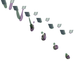
Figure 2. Evolution of the binary droplet collision. (a) Example of a time sequence of a binary droplet collision and its mixing process. The two liquids, L1 and L2, are shown by the isosurface  $\alpha _i = 1/2$, $i = 1,2$ in green and purple, respectively, and the contact surface area is highlighted in grey. (b) Evolution of the volume of the liquids (top) and their flow rate (bottom). The delay in the injection time and the velocity difference are indicated by ${\rm \Delta} t_0$ and ${\rm \Delta} U_{nzl}$. The temporal coordinate has been shifted, identifying $t = 0$ as the time of contact.
The concentration fields  $\alpha _1$ and $\alpha _2$ take the value 1 at the $+x_{nzl}$ and $-x_{nzl}$ inlets, and zero everywhere else on the top boundary, respectively. This is prescribed by means of the auxiliary function $G$:
$G$:
 \begin{equation} \alpha_1(\boldsymbol{x}) = \begin{cases} 1 & \mathrm{if} \ G(\boldsymbol{x}; -x_{nzl}, \theta + {\rm \Delta} \theta, \varphi + {\rm \Delta} \varphi) \geq 0, \\ 0 & \mathrm{otherwise}, \end{cases} \end{equation}
and
 \begin{equation} \alpha_2(\boldsymbol{x}) = \begin{cases} 1 & \mathrm{if} \ G(\boldsymbol{x}; +x_{nzl}, \theta, \varphi) \geq 0, \\ 0 & \mathrm{otherwise}. \end{cases} \end{equation}
3. Methods and analysis
The coupled system of advection–diffusion and momentum conservation equations in (2.2)–(2.4) is solved in an open-source, finite-volume solver with multiphase capabilities, OpenFOAM (Weller et al. Reference Weller, Tabor, Jasak and Fureby1998). We carry out direct numerical simulations using a second-order scheme for both temporal advancement and spatial discretisation.
The advection–diffusion equations for the concentration fields, (2.2) and (2.3), were solved using volume-of-fluid with the MULES algorithm for two sub-cycles with interface compression coefficient  $c_\alpha = 1.5$. The momentum equation (2.4) is solved using the PISO-SIMPLE algorithm for the coupling of the pressure and velocity fields. The pressure is solved by an over-relaxation method with relative tolerance $10^{-7}$ for the pressure correction and $10^{-9}$ for the final pressure solution.
As can be observed in figure 1(b), the simulation domain consists of a cubic volume of  $8$ mm width, meshed with hexahedral cells with four levels of refinement, duplicating the density of cells approaching the path drawn by the liquids. The largest cell type is $h = 250\ \mathrm {\mu }$m in width, which corresponds to $1/32^3$ of the domain volume, and the smallest cell type is $h = 15.625\ \mathrm {\mu }$m in width, or $1/512^3$ of the total volume. The mesh is refined progressively such that the Kolmogorov length scale (Pope Reference Pope2000), $\eta$, is maintained above the local cell size, $h$, that is, $\min \{\eta / h\} \approx 2.10 > 1$ for all $\boldsymbol {x} \in \varOmega$ and $t$. The increment for temporal advancement, ${\rm \Delta} T$, is adaptive in order to keep the Courant number, $\mathit{Co}$, below $0.1$, which, on average, resulted in ${\rm \Delta} T \sim 0.1\ \mathrm {\mu }$s.
To ensure that the parasitic currents (Harvie, Davidson & Rudman Reference Harvie, Davidson and Rudman2006) do not affect the simulation results, a different set of simulations was carried out. These consisted of a three-dimensional liquid droplet of radius  $R_{nzl}$ suspended in air with the material properties reported in table 1 and a homogeneous mesh resolution $h = 15.625\ \mathrm {\mu }$m to match the main simulations. The kinetic energy and asphericity of the droplet are evaluated after the system arrived at a static configuration. It was found that the maximum magnitude of the parasitic currents reach at most up to $0.05\ {\rm m} \ {\rm s}^{-1}$, which is two orders of magnitude smaller compared to the characteristic velocity of the main simulations. Moreover, most of the analysis of the flows in the present study will be performed at the interface of the two miscible liquids where the surface tension is zero, thus this manifold does not produce parasitic currents. The asphericity, measured as the relative variance of the distance of the points in the isosurface $\alpha _1 = 1/2$ against the ideal droplet radius $R_{nzl}$, was found to be $2.3 \times 10^{-4}$. In conclusion, the numerical errors, arising from the discretisation of surface tension force, are negligible. We begin the simulations at $t = 0$, and they run until the droplets come out of the simulation domain, which occurs in less than $10$ ms. However, in what follows, we have shifted the time variable such that contact between the droplets occurs at zero, i.e. $t \rightarrow t - t_c$, where $t_c$ is the instant of first contact, as shownin figure 2(a).
For the parameters specified in table 1, the typical Weber number  $We := 2 \rho R_{nzl} u_r^2 / \sigma$ found in the simulations was $We < 25$, thus we expected a slow coalescence resulting from the collision at small values of the impact parameter. The choice in the parameter ranges for the current analysis is influenced by the experimental set-up of da Conceicao Ribeiro et al. (Reference da Conceicao Ribeiro, Pal, Ferreira, Gentile, Benning and Dalgarno2018). On the one hand, the range of values for ${\rm \Delta} t_0$ and ${\rm \Delta} U_{nzl}$ is unbounded for such devices. However, we observed that ${\rm \Delta} t_0 \in [-5/16, 5/16]$ and ${\rm \Delta} U_{nzl} \in [-0.8, 0.8] \ {\rm m} \ {\rm s}^{-1}$ resulted in $B \lesssim 1$, i.e. contact between droplets. On the other hand, the angles for the alignment of the nozzle, ${\rm \Delta} \theta$ and ${\rm \Delta} \varphi$, are within the degrees of freedom of such types of bioprinters. These allow for adjustments that compensate for other sources of misalignment.
We will now focus on the quantification of mixing, but first, let us briefly estimate the state of turbulence of both the gas and liquid phases. Following Pope (Reference Pope2000), let us define the Reynolds number in the gas phase as  $Re_g := U_g L_g / \nu _g$, where $U_g := \max _{gas} |\boldsymbol {u}|$ is the maximum velocity in the gas phase, and $L_g := 2 U_g^3 / (\nu _g \max _{gas}\,|\boldsymbol {\nabla } \times \boldsymbol {u}|^2)$ defines the characteristic length scale. It was found that the typical values for $Re_g$ were approximately $10^3$, suggesting a weakly turbulent flow in the gas phase. For the liquid phase, we define $Re_l := k^2 / \nu _l \epsilon$, where $k := \overline {\boldsymbol {u}' \boldsymbol {\cdot } \boldsymbol {u}'}/2$ is the turbulence kinetic energy, and $\epsilon := 2 \nu _l \, \mathrm {tr}\, \overline {{\boldsymbol{\mathsf{S}}}'^2}$ is the dissipation; the overbar corresponds to the Reynolds average, $\boldsymbol {u}' := \boldsymbol {u} - \bar {\boldsymbol {u}}$ and ${\boldsymbol{\mathsf{S}}}' := (\boldsymbol {\nabla } \boldsymbol {u}' + \boldsymbol {\nabla } \boldsymbol {u}'^{\rm T}) / 2$. To estimate $Re_l$, we approximate $\bar {\boldsymbol {u}}$ by the velocity of the centre of mass of the liquid phase. This is an asymptotic approximation that, due to the large dynamic viscosity ratio between the two immiscible phases, is mostly accurate. It was found that the typical values at the instant of first contact between the droplets reached $Re_l \sim 10^3$, decaying to $Re_l \sim 200$ shortly after. Therefore, in contrast to the gas phase, this suggests a quasi-laminar flow. Although not conclusive, this analysis may give us an idea of the state of turbulence of both phases, and thus the tendency for mixing.
3.1. Quantifying mixing
We are interested in the continuous process in which mixing takes place. Therefore, to quantify partial mixing, let us define the segregation parameter between liquids L1 and L2 as
 \begin{equation} \chi := \frac{\langle \alpha_i^{2} \rangle - \langle \alpha_i \rangle^2}{\langle \alpha_i \rangle\,(1 - \langle \alpha_i \rangle)} = 1 - \frac{V_1 + V_2}{V_1 V_2} \int_{\varOmega_l} \alpha_1\alpha_2 \,\mathrm{d} V, \end{equation}
where, without loss of generality,  $i = 1$ or $i = 2$ can be chosen and using (2.1) leads to the last equality in (3.1). Here, the operation $\langle \cdot \rangle$ computes the volume average in $\varOmega _l$, where $\alpha _3$ is zero. Since the concentration is a conserved quantity for passive scalar mixing, any diffusive flux is assumed to be zero at the liquid–gas interface. It follows that $\langle \alpha _i \rangle = V_i / (V_1 + V_2)$, where $V_i$ is the total volume of liquid $i$ injected.
As the name suggests,  $\chi = 0$ corresponds to an absence of variance in concentration, which implies a homogeneous or complete mixture. Conversely, $\chi = 1$ corresponds to a state in which the regions occupied by the liquids L1 and L2 do not intersect (Doering & Thiffeault Reference Doering and Thiffeault2006; Foures et al. Reference Foures, Caulfield and Schmid2014; Thiffeault Reference Thiffeault2021). The transport equation of the segregation parameter can be deduced by taking the material derivative and using (2.2), which results in
 \begin{equation} \frac{\mathrm{d}\chi}{\mathrm{d}t} ={-}2\,\frac{V_1 + V_2}{V_1 V_2} \int_{\varOmega_l} N \,\mathrm{d} V, \end{equation}
where  $N := D\,|\boldsymbol {\nabla } \alpha _1|^2$, the integrand in the right-hand side of (3.2), corresponds to the scalar dissipation rate.
The scalar dissipation rate  $N$ is a positive quantity, proportional to the rate of entropy production by diffusion, which indicates the irreversibility of a mixing process (Davidson Reference Davidson2015). The transport equation of $N$ is given by (Chakraborty et al. Reference Chakraborty, Champion, Mura and Swaminathan2011)
 \begin{equation} \frac{\mathrm{d}N}{\mathrm{d}t} = \boldsymbol{\nabla} \boldsymbol{\cdot} (D\,\boldsymbol{\nabla} N) - 2 D^2\,|\boldsymbol{\nabla} \boldsymbol{\nabla} \alpha_1|^2 - 2 N {\boldsymbol{\mathsf{S}}} : \hat{\boldsymbol{n}}_{c}\hat{\boldsymbol{n}}_{c}, \end{equation}
where  $\mathrm {d} / \mathrm {d} t := (\partial _t + \boldsymbol {u} \boldsymbol {\cdot } \boldsymbol {\nabla })$ is the material derivative and $\hat {\boldsymbol {n}}_{c} := \boldsymbol {\nabla } \alpha _1 / |\boldsymbol {\nabla } \alpha _1|$ is the unit normal vector of the contact surface. The first term in the right-hand side of (3.3) corresponds to the contribution by the fluxes driven by gradients of $N$. The second term is dubbed the molecular dissipation rate and represents a sink term. The last term in the right-hand side of (3.3) is called the scalar–turbulence interaction term and models the contribution by the stretching of the flow; it can be expressed in terms of the eigenvalues $\{\lambda _i \}_{i = \alpha, \beta, \gamma }$ and eigenvectors $\{ \hat {\boldsymbol {e}}_i \}_{i = \alpha, \beta, \gamma }$ of ${\boldsymbol{\mathsf{S}}}$ (Dresselhaus & Tabor Reference Dresselhaus and Tabor1992):
 \begin{equation} {\boldsymbol{\mathsf{S}}} : \hat{\boldsymbol{n}}_{c}\hat{\boldsymbol{n}}_{c} = \sum_{i = \alpha, \beta, \gamma} (\hat{\boldsymbol{n}}_{c} \boldsymbol{\cdot} \hat{\boldsymbol{e}}_i)^2 \lambda_i. \end{equation}
 Both the segregation parameter and the scalar dissipation rate are mixing measures of the type  $\langle | \boldsymbol {\nabla }^m \alpha _i |^2 \rangle$, for $m = 0, 1$ (Doering & Thiffeault Reference Doering and Thiffeault2006).
To keep track of the region where the mixing takes place, one can define the contact surface area (Vervisch et al. Reference Vervisch, Bidaux, Bray and Kollmann1995) between the two liquids,
 \begin{equation} S_{c} := \int_{\varOmega_l} | \boldsymbol{\nabla} \alpha_1 | \,\mathrm{d} V. \end{equation}
As for any diffusive process, the total mixing rate is proportional to the surface area; therefore, the higher the  $S_{c}$, the quicker the segregation parameter will decrease. The evolution of the contact area is governed by the transport equation
 \begin{equation} \frac{\mathrm{d}S_{c}}{\mathrm{d}t} ={-} D \int_{\varOmega_l} \frac{|\boldsymbol{\nabla} \boldsymbol{\nabla} \alpha_1|^2}{|\boldsymbol{\nabla} \alpha_1|} \,\mathrm{d} V - \sum_{i = \alpha, \beta, \gamma} \int_{\varOmega_l} (\hat{\boldsymbol{n}}_{c} \boldsymbol{\cdot} \hat{\boldsymbol{e}}_i)^2 \lambda_i\, |\boldsymbol{\nabla} \alpha_1| \,\mathrm{d} V, \end{equation}
3.2. Analysis of the flow structure
To understand the effect that convective flows have in mixing, and in particular, on the terms described in (3.4), the flow field will be analysed in the region of contact between the two liquids. For that, the behaviour of the strain-rate tensor,  ${\boldsymbol{\mathsf{S}}}$, and, more generally, the velocity gradient tensor, ${\boldsymbol{\mathsf{A}}} := \boldsymbol {\nabla } \boldsymbol {u}$, will be analysed.
To illustrate the meaning of  ${\boldsymbol{\mathsf{A}}}$, consider a virtual swarm of particles at some position $\boldsymbol {y}$ in a small region around $\boldsymbol {x}$ in the three-dimensional Cartesian space that are advected by the flow field $\boldsymbol {u}$. Suppose that the motion of the particles is given by $\mathrm {d} \boldsymbol {y} / \mathrm {d} t = \boldsymbol {u}(\boldsymbol {y})$, and assume that $\boldsymbol {u}$ is continuous around $\boldsymbol {x}$. Then, $\mathrm {d} \boldsymbol {y} / \mathrm {d} t \approx \boldsymbol {u}(\boldsymbol {x}) + (\boldsymbol {y} - \boldsymbol {x}) \boldsymbol {\cdot } {\boldsymbol{\mathsf{A}}}(\boldsymbol {x})$. This implies that $\boldsymbol {u}(\boldsymbol {x})$ corresponds to the background motion of the virtual particles, whilst ${\boldsymbol{\mathsf{A}}}$ describes their relative motion. Therefore, by means of the velocity gradient tensor, we can analyse the local flow field at $\boldsymbol {x}$ such as the flow topology and the eigenvectors and eigenvalues of ${\boldsymbol{\mathsf{A}}}$ (Chong, Perry & Cantwell Reference Chong, Perry and Cantwell1990; Meneveau Reference Meneveau2011).
The eigenvalues of  ${\boldsymbol{\mathsf{A}}}$ correspond to the roots of the characteristic polynomial $\det (\boldsymbol{\mathsf{A}} - \lambda ' \boldsymbol{\mathsf{I}}) = \lambda '^3 + P \lambda '^2 + Q \lambda ' + R$. The coefficients $P$,
$P$,  $Q$ and $R$ are called the first, second and third invariants of the transformation, and are given by
 $$\begin{gather} P ={-} \mathrm{tr}\, {\boldsymbol{\mathsf{A}}} ={-} \sum_i \lambda_i' \ (= 0\ \mathrm{due\ to\ incompressibility}), \end{gather}$$
 $$\begin{gather}Q = \tfrac{1}{2} [ (\mathrm{tr}\ {\boldsymbol{\mathsf{A}}})^2 - \mathrm{tr}\ {\boldsymbol{\mathsf{A}}}^2 ] = \lambda_1'\lambda_2' + \lambda_2'\lambda_3' + \lambda_3'\lambda_1' , \end{gather}$$
 $$\begin{gather}R ={-} \det {\boldsymbol{\mathsf{A}}} ={-} \prod_i \lambda_i'. \end{gather}$$
We have used the primed notation to emphasise the difference between the eigenvalues of  ${\boldsymbol{\mathsf{S}}}$ and those of ${\boldsymbol{\mathsf{A}}}$. Since ${\boldsymbol{\mathsf{S}}}$ is a symmetric tensor, the eigenvalues are real and the eigenvectors are orthogonal, which is not the case for the eigenvalues and eigenvectors of ${\boldsymbol{\mathsf{A}}}$. To distinguish when the eigenvalues are real-valued or have an imaginary part, let us define the discriminant
 \begin{equation} \varDelta := \frac{R^2}{4} + \frac{Q^3}{27}. \end{equation}
If  $\varDelta \leq 0$, then all three eigenvalues are real; however, if $\varDelta > 0$, then $\boldsymbol{\mathsf{A}}$ has one real and two complex eigenvalues. If the eigenvalues have an imaginary part, then the nearby trajectories spiral inwards or outwards from the observation point $\boldsymbol {x}$. The real part of the eigenvalues reveals the stability at the observation point. From (3.7), it follows that the real parts of the eigenvalues cannot have the same sign, i.e. one must be positive, one must be negative, and an intermediate one can have either sign. A negative eigenvalue indicates that trajectories are attracted towards the observation point whereas positive indicates that they are repelled. Consequently, the sign of $R$ determines the number of stable and unstable manifolds around the observation point, and when $R = 0$, the linear approximation may not be enough to determine the local stability at $\boldsymbol {x}$.
We classify the topology of the flow as follows (Chong et al. Reference Chong, Perry and Cantwell1990).
(i) ${S1}$, $\varDelta > 0$ and $R > 0$, consists of a one-dimensional (1-D) compressive manifold combined with a two-dimensional (2-D) unstable manifold that spirals away from the focal point.
(ii)
${S2}$, $\varDelta \leq 0$ and $R > 0$, 1-D compressive and 2-D expansive manifolds.(iii)
${S3}$, $\varDelta \leq 0$ and $R < 0$, 1-D expansive and 2-D compressive manifolds.(iv)
${S4}$, $\varDelta > 0$ and $R < 0$, 1-D stretching and 2-D stable focus manifolds.


Furthermore, the topologies  $S1$ and $S4$ can be subdivided depending on the sign of $Q$, that is, $S1^+$ and $S1^-$ ( $S4^+$ and $S4^-$) for $Q \geq 0$ and $Q < 0$, respectively. The representative flows are sketched in figure 3(a) and their corresponding regions in the $Q$–
$Q$– $R$ space in figure 3(b).

Figure 3. Flow topology and dynamics in the  $Q$–
$Q$– $R$ phase space. (a) Schematic colour-coded classification of the flow topology. The solid black lines correspond to streamlines beginning at the empty circles. The brown and green arrows represent the equal- and opposite-sign manifolds of the vector field, respectively. (b) The streamlines show the trajectories of the restricted Euler system, and the colours indicate the different flow topology regions.
The invariants  $Q$ and $R$ follow the equations of motion away from the interfaces (Martin et al. Reference Martin, Ooi, Chong and Soria1998):
 $$\begin{gather} \frac{\mathrm{d}R}{\mathrm{d}t} = \frac{2}{3}\, Q^2 - \mathrm{tr} ({\boldsymbol{\mathsf{A}}}^2 {\boldsymbol{\mathsf{H}}}) - \nu \, \mathrm{tr} ({\boldsymbol{\mathsf{A}}}^2\,\nabla^2 {\boldsymbol{\mathsf{A}}}), \end{gather}$$
 $$\begin{gather}\frac{\mathrm{d}Q}{\mathrm{d}t} ={-}3 R - \mathrm{tr} ({\boldsymbol{\mathsf{A}}} {\boldsymbol{\mathsf{H}}} ) - \nu \, \mathrm{tr} ( {\boldsymbol{\mathsf{A}}}\,\nabla^2 {\boldsymbol{\mathsf{A}}} ), \end{gather}$$
where  ${\boldsymbol{\mathsf{H}}}:= - (\boldsymbol {\nabla } \boldsymbol {\nabla } p - {\boldsymbol{\mathsf{I}}}\,\nabla ^2 p / 3) / \rho$ is the anisotropic pressure Hessian. The last two terms in both (3.11) and (3.12) are non-local, thus depend on the boundary conditions and the capillary forces at the liquid–gas interface. The terms proportional to $\nu$ in (3.11) and (3.12) are derived from the viscous dissipation term in the Navier–Stokes equation, thus act as sinks.
To understand the dynamics of the system in (3.11) and (3.12), let us first consider the restricted Euler system that assumes that  ${\boldsymbol{\mathsf{H}}} + \nu \,\nabla ^2 {\boldsymbol{\mathsf{A}}}$ is negligible. This corresponds to a state in which the pressure is isotropic and viscous damping is negligible. In this case, (3.11) and (3.12) are reduced to a closed and autonomous dynamical system whose phase space portrait is depicted in figure 3(b). At the origin ( $R = 0$ and $Q = 0$), a half-stable fixed point is found, and the surrounding trajectories evolve from $R < 0$ to $R > 0$ and points in the $\varDelta = 0$ manifold stay in it. This implies that the natural tendency of the reduced dynamical system is to separate the rotation-dominated from the strain-dominated regions, and the evolution takes states from $R < 0$ to $R> 0$. In other words, the ${S4}$ and ${S3}$ topologies are turning into the ${S1}$ and ${S2}$ topologies, respectively (Martin et al. Reference Martin, Ooi, Chong and Soria1998).
Furthermore, far from interfaces, the transport equations of enstrophy and strain-rate production can be expressed in terms of the invariants
 \begin{equation} \frac{\mathrm{d}\zeta}{\mathrm{d}t} = 4(R_S - R) + \nu \boldsymbol{\omega} \boldsymbol{\cdot} \nabla^2 \boldsymbol{\omega}, \end{equation}
where  $\zeta := |\boldsymbol {\omega }|^2/2$ is the enstrophy and $\boldsymbol {\omega } := \boldsymbol {\nabla } \times \boldsymbol {u}$ is the vorticity, and
 \begin{equation} \frac{\mathrm{d} Q_S}{\mathrm{d} t} ={-}2 R_S - R - \frac{1}{\rho}\, \mathrm{tr}\, {\boldsymbol{\mathsf{S}}} \boldsymbol{\nabla} \boldsymbol{\nabla} p - \nu \, \mathrm{tr}\, {\boldsymbol{\mathsf{S}}}\,\nabla^2 {\boldsymbol{\mathsf{S}}}, \end{equation}
where  $Q_S := -\mathrm {tr}\, {\boldsymbol{\mathsf{S}}}^2/2$ and $R_S := -\det {\boldsymbol{\mathsf{S}}}$ are the second and third invariants of the strain rate, respectively. Therefore, for the restricted Euler system, (3.13) and (3.14) can be combined into
 \begin{equation} \frac{\mathrm{d}}{\mathrm{d}t} \left( \frac{\epsilon}{\nu} \right) = 12 R + 2\, \frac{\mathrm{d}\zeta}{\mathrm{d}t}, \end{equation}
where  $\epsilon := -4 \nu Q_S$ is the instantaneous dissipation rate of kinetic energy.
This concludes the conceptual framework that will support the analysis of our numerical simulations that will follow. However, before proceeding, these tools will be used for a similar system where an analytic approximation is available.
3.3. Axisymmetric collision of identical spherical droplets
To illustrate the concepts introduced previously, let us consider the case of an axisymmetric binary droplet collision of identical droplets. Following Roisman (Reference Roisman2004), after the first contact and during the initial stages of the collision, the droplets undergo a deformation in which the flow field in the vicinity of the contact surface is well approximated by
 $$\begin{gather} u_x \approx \frac{u_r x}{2 l^3}\,(4 x^2 - 3 l^2), \end{gather}$$
 $$\begin{gather}u_\xi \approx \frac{3 u_r}{4 l^3}\,\xi (l^2 - 4 x^2), \end{gather}$$
where  $x$ is the coordinate that runs parallel to the axis of symmetry, $\xi = (y^2 + z^2)^{1/2}$ is the distance from the axis, $u_r$ is the magnitude of the relative velocity and $l$ is the thickness of the liquid lamella that forms by radial expansion of the droplets at early stages. Then the velocity gradient tensor is given by
 \begin{equation} {\boldsymbol{\mathsf{A}}} = \frac{3 u_r}{4 l^3} \begin{pmatrix} - 2(l^2 - 4 x^2) & 0 & 0 \\ - 8 x y & (l^2 - 4 x^2) & 0 \\ - 8 x z & 0 & (l^2 - 4 x^2) \end{pmatrix}. \end{equation}
At the plane of collision  $x = 0$, ${\boldsymbol{\mathsf{A}}}$ reduces to a diagonal matrix whose second and third invariants are given by
 \begin{equation} R(x = 0) = \frac{27 u_r^3}{32 l^3} \quad \mathrm{and} \quad Q(x = 0) ={-}\frac{27 u_r^2}{16 l^2}.\end{equation}
The evaluation of the discriminant from the characteristic equation (3.10) shows that  $\varDelta = 0$, which corresponds to an ${S2}$ topology flow.
In this stage of the collision, the contact surface area is increasing due to the stretching motion of the flow. The scalar–turbulence interaction term evaluates to
 \begin{equation} - 2 {\boldsymbol{\mathsf{S}}}: \hat{\boldsymbol{n}}_c \hat{\boldsymbol{n}}_c = \frac{3}{l}\,u_r \sim \frac{1}{N}\,\frac{\mathrm{d}N}{\mathrm{d}t}, \end{equation}
where the last relation is based on (3.3). This estimates an exponential growth rate of the scalar dissipation rate, and consequently the contact surface area.
The growth of the contact surface area cannot carry on indefinitely due to surface tension and viscous forces. Surface tension reverses the direction of the flow in a periodic fashion, leading to oscillations in the contact surface area, whilst viscous stresses dampen the motion of the flow (Roisman Reference Roisman2009; Roisman, Berberović & Tropea Reference Roisman, Berberović and Tropea2009).
4. Results and discussion
The simulation parameters considered for the present analysis are summarised in table 1 and are inspired by a bioprinting set-up (da Conceicao Ribeiro et al. Reference da Conceicao Ribeiro, Pal, Ferreira, Gentile, Benning and Dalgarno2018). To investigate the effects of differences in the configuration of the L1 inlet relative to L2, the simulations were run in four different batches: (i) varying the injection velocity,  ${\rm \Delta} U_{nzl}$; (ii) varying the relative injection time, ${\rm \Delta} t_0$; (iii) introducing a difference in the polar angle by ${\rm \Delta} \theta$; and (iv) changing the azimuth angle ${\rm \Delta} \varphi$.
Additionally, to illustrate the combined effect of these configuration parameters in the dynamics of the droplet collision and mixing for an asymmetric collision presented in figures 2, 8 and 9, we set  ${\rm \Delta} U_{nzl} = 0.24\ {\rm m} \ {\rm s}^{-1}$, ${\rm \Delta} t_0 = T_{pulse}/4, {\rm \Delta} \theta = -4^{\circ }$ and ${\rm \Delta} \varphi = 6^{\circ }$. This is to contrast against the symmetric collision presented in figures 6 and 7, in which these configuration parameters are equal to zero ( ${\rm \Delta} U_{nzl} = {\rm \Delta} t_0 = {\rm \Delta} \theta = {\rm \Delta} \varphi = 0$).
4.1. Impact of non-spherical droplets
It can be observed from figure 2(a) that the droplets do not have a spherical shape, in contrast to many studies of binary droplet collisions, but are rather elongated in the direction of motion relative to their respective nozzles. As expected, the contact point of the droplets would produce different outcomes depending on the shape of the droplet; the dimensionless impact parameter  $B$, as defined for spherical droplets (Ashgriz & Poo Reference Ashgriz and Poo1990; Al-Dirawi & Bayly Reference Al-Dirawi and Bayly2019), cannot be used to represent the off-centred collision in this work.
In the following, we generalise the definition of the dimensionless impact parameter for droplets that are non-spherical and continuously evolving. We will base our definition on the underlying concept of the traditional expression as stated in § 1.
Since the shape of the droplets is changing in time, the impact parameter is meaningful only at  $t = 0$, which corresponds to the moment of first contact. The relative velocity between the two droplets is $\boldsymbol {u}_r := \boldsymbol {U}_1 - \boldsymbol {U}_2$, where $\boldsymbol {U}_i$ is the velocity of the centre of mass of droplet $i$. The vector $\boldsymbol {u}_r$ and the first contact point between the two liquids create the contact plane (see figure 4a). The shape of the droplets is then projected onto the contact plane, and if their projected images intersect, then the droplets are bound to collide; otherwise, they pass each other without contact.

Figure 4. Calculation of the impact parameter. (a) Example of an asymmetric collision between two droplets at the moment of first contact that illustrates the construction of the dimensionless impact parameter  $B$. (b) The impact parameter is evaluated at different set-up configurations (symbols) and the fitting of the curve in (4.9) applied to each case (solid line).
The distance between the centre of mass of the droplets on the contact plane,  $b := |\boldsymbol {b}|$, is defined such that
 \begin{equation} \boldsymbol{b} := (\boldsymbol{X}_1 - \boldsymbol{X}_2) \times \frac{\boldsymbol{u}_r}{|\boldsymbol{u}_r|}, \end{equation}
where  $\boldsymbol {X}_i$, $i = 1, 2$, are the centres of mass of the liquids L1 and L2, respectively. Let $P_i$, $i = 1, 2$, be the projected image of droplet $i$ onto the contact plane. Then, let $C = \bigcap _i P_i$ be the set of points at the intersection. As illustrated in figure 4(a), we measure the depth of the overlap between the projections, $c$, by finding the longest line in $C$ that is parallel to $\boldsymbol {b}$, formally,
 \begin{equation} c := \max \{ c' : c' \boldsymbol{b}/b = (\boldsymbol{x}_2 - \boldsymbol{x}_1); \boldsymbol{x}_1,\boldsymbol{x}_2 \in C \}, \end{equation}
and  $c = 0$ if $C = \emptyset$. In this way, the generalised dimensionless impact parameter can be defined as
 \begin{equation} B := \frac{b}{b + c}. \end{equation}
Note that  $b \ge 0$ and $c \ge 0$ and if $b = 0$, then $c \neq 0$; this implies that $0 \leq B \leq 1$, where $B = 0$ corresponds to a head-on collision, and $B = 1$, which occurs if $c = 0$, implies that the droplets do not make contact during their trajectories at any time.
For spherical droplets of diameter  $d_i$, the depth of the overlap reduces to $c = (d_1 + d_2) / 2 - b$ and we recover the usual expression $B = 2 b / (d_1 + d_2)$.
Let us anticipate the functional dependence of  $B$ after a small deviation from the head-on collision. This can be done by performing a small deviation around the head-on collision for the terms $b$ and $c$ in (4.3). Therefore, an expression can be obtained by considering
 \begin{equation} B \sim \frac{b_0 + {\rm \Delta} b}{b_0 + {\rm \Delta} b + c_0 + {\rm \Delta} c} \sim \frac{{\rm \Delta} b}{c_0}, \end{equation}
where  $b_0$ and $c_0$ are the values for the head-on collision, and ${\rm \Delta} b$ and ${\rm \Delta} c$ represent their variation from the parameters that introduce the asymmetry ( ${\rm \Delta} U_{nzl}, {\rm \Delta} t_0, {\rm \Delta} \theta$ and ${\rm \Delta} \varphi$) up to linear order. The last relation in (4.4) is obtained recalling $b_0 = 0$ for the head-on collision.
The expressions for  ${\rm \Delta} b$ and $c_0$ can be estimated by assuming that the droplets have the morphology of a cylindrical rod of radius $R_{nzl}$ and length $\ell _1 = T_{pulse} (U_{nzl} + {\rm \Delta} U_{nzl})$ and $\ell _2 = T_{pulse} U_{nzl}$ for liquids L1 and L2. Here, $c_0$ corresponds to the overlapping length in the direction of $\boldsymbol {b}$. However, in the head-on collision case, $c_0$ is degenerate since $\boldsymbol {b} = 0$, thus it can take the two values depending on the source of asymmetry:
 \begin{equation} c_0 \approx \begin{cases} 2 R_{nzl} & \text{if } {\rm \Delta} \varphi \neq 0, \\ U_{nzl} T_{pulse} \cos \theta & \text{otherwise}. \end{cases} \end{equation}
To calculate  ${\rm \Delta} b$, we can approximate the positions of the centres of mass of the two droplets as
 \begin{equation} \boldsymbol{X}_1 \approx (t - {\rm \Delta} t_0 - T_{pulse}/2 ) (U_{nzl} + {\rm \Delta} U_{nzl})\,\hat{\boldsymbol{J}}(\theta + {\rm \Delta} \theta, {\rm \Delta} \varphi) - x_{nzl} \hat{\boldsymbol{e}}_x \end{equation}
and
 \begin{equation} \boldsymbol{X}_2 \approx (t - T_{pulse}/2 ) U_{nzl} \hat{\boldsymbol{J}}(\theta, {\rm \pi}) + x_{nzl} \hat{\boldsymbol{e}}_x. \end{equation}
The relative velocity of the droplets is given by  $\boldsymbol {u}_r = \mathrm {d} (\boldsymbol {X}_1 - \boldsymbol {X}_2) / \mathrm {d}t$. Then, by substituting (4.6) and (4.7) in (4.1), and keeping terms up to linear order, it can be shown that
 \begin{align} \frac{{\rm \Delta} b}{c_0} = \left[ \left( \frac{{\rm \Delta} t_0}{T_{pulse}} \right)^2 + \left( \frac{x_{nzl}}{U_{nzl} T_{pulse}} \right)^2 \left( \frac{{\rm \Delta} \theta^2}{\cos^2 \theta} + \frac{{\rm \Delta} U_{nzl}^2}{U_{nzl}^2 \sin^2 \theta} \right) + \left( \frac{x_{nzl}\,{\rm \Delta} \varphi}{2 R_{nzl}} \right)^2 \right]^{1/2}. \end{align}
 In figure 4, the value of the impact parameter calculated from the simulation results is presented. Guided by (4.8), we propose an empirical approximation to  $B$ that captures its general trend by varying each parameter:
 \begin{align} B \approx \left[c_t \tan^2 \frac{{\rm \Delta} t_0 }{b_t T_{pulse}} + (c_\theta\,{\rm \Delta} \theta + d_\theta\,{\rm \Delta} \theta^2)^2 + (c_u ({\rm \Delta} U_{nzl} / U_{nzl})^{n} - 1 )^2 + (c_\varphi\,{\rm \Delta} \varphi )^2 \right]^{1/2}, \end{align}
where each of the constants is found by least squares optimisation. Varying  ${\rm \Delta} U_{nzl}$, we find that $n = 0.4$ and $c_u = 1.43$; varying ${\rm \Delta} t_0$, gave the constants $b_t = 0.26$ and $c_t = 0.12$. Varying the angles ${\rm \Delta} \theta$ and ${\rm \Delta} \varphi$ resulted in $c_\theta = 0.018\ {\rm rad}^{-1}$ and $d_\theta = 43.2\ {\rm rad}^{-2}$, and $c_\varphi = 2.25\ {\rm rad}^{-1}$, respectively.
Figure 5(a) shows the evolution of the segregation parameter  $\chi$ and the scalar dissipation rate $N$. As the droplets collide, the mixing process begins and the segregation parameter decreases. The scalar dissipation rate shows a fast increase after the first contact between the droplets. Soon after, it arrives at a local maximum, which is reflected as an inflection point in $\chi$ at $t = 1.575$ ms and $t = 1.425$ ms for the symmetric and asymmetric collisions, respectively. From that instant onwards, $\chi$ will decrease at a lower rate. A similar behaviour was observed in all our simulations.

Figure 5. Quality of the mixing process after breaking the symmetry of the collision. (a) Evolution of the segregation parameter (solid line) and scalar dissipation rate (dashed line) for a symmetric and an asymmetric collision. (b) Evaluation of the segregation parameter after  $4$ ms after first contact for injection velocity difference, injection time difference, and polar and azimuthal angles. (c) Segregation as a function of the impact parameter for all simulations. The solid line is an approximation to the common trend followed by all the points, except for those corresponding to ${\rm \Delta} \varphi$.
In figure 5(b), the segregation parameter at  $t = 4\ {\rm ms} = 1.6 T_{pulse}$, the evaluation time, is shown for all simulation results. The evaluation time is chosen as the maximum time lapse after the collision that is common to all simulations. In other words, it is the longest interval of time for the mixing process to take place before the liquids exit the simulation domain. Since $\chi$ is a monotonically decreasing function of time, the results are similar at any other evaluation time of choice.
The four plots in figure 5(b) show the influence of the different configuration parameters in the mixing process. It can be observed from figure 5(b) that decreasing the velocity of the inlet has a strong effect on  $\chi$ and reducing the velocity by ${\sim }15\,\%$ gives a near-optimal mixing; however, decreasing by ${\sim }40\,\%$ raises $B$ to $B = 1$, and mixing is absent. In contrast, increasing the velocity has a smaller effect, where the optimal mixing is found at a ${\sim }32\,\%$ increase in the inlet velocity.
The difference in injection time shows a fast improvement in the quality of the mixing, reaching an optimal mixing at  $|{\rm \Delta} t_0| = 0.12 T_{pulse}$, which afterwards start deteriorating until $|{\rm \Delta} t_0| = 0.3 T_{pulse}$, when the droplets barely touch each other.
Changes in the polar and azimuthal angles,  ${\rm \Delta} \theta$ and ${\rm \Delta} \varphi$, show an improvement in the mixing quality when breaking the symmetry of the collision. However, varying the azimuthal angle has a smaller improvement on the mixing even though the impact parameter is found to increase at a higher rate.
In summary, it can be observed in figure 5(c) that the segregation parameter is strongly dependent on the impact parameter. Over a finite time, the segregation parameter shows a high value for the symmetric collision; this is not the exception, but rather the common trend for different sources of asymmetry. The segregation parameter decreases, reaching a wide minimum at  $B = 0.2 \pm 0.1$ in which optimal mixing occurs. For higher values of the impact parameter, mixing deteriorates. The overall tendency is captured by the function
 \begin{equation} \chi \approx a_\chi B \ln \frac{B}{b_\chi} + \chi_0, \end{equation}
where the constants  $a_\chi = 2.23$ and $b_\chi = 0.551$ are found by least squares optimisation, and $\chi _0 = 0.734$ is the value of the segregation parameter for the symmetric collision. The function in (4.10) has its global minimum at $B = b_\chi / {\rm e} \approx 0.203$, where ${\rm e}$ is the base of the natural logarithm. This is true except for the set of simulations where ${\rm \Delta} \varphi \neq 0$. As can be observed, the segregation parameter does not decrease as much as the other cases. This does not imply that the definition of the impact parameter is inadequate. As will be discussed later, the system exhibits a deeper-level complexity, which is reflected in the infeasibility of reaching a near optimal state of mixing.
4.2. Evolution of the topology of the flow and the contact surface
To better understand why optimal mixing occurs for  $B \neq 0$, we will explore in more detail the evolution of the contact surface and the flows in its vicinity.
Figure 6(a) shows the contact surface of a symmetric binary droplet collision. This corresponds to the isosurface  $\alpha _1 = 1/2$ at two different times: $t = 0.5$ ms and $t = 2$ ms. It can be observed from figure 6(a) that the contact surface is flat, which is due to the reflexive symmetry of the system. The contact surface between the two liquids occurs at the mirror plane $x = 0$. This implies that $\hat {\boldsymbol {n}}_c = \hat {\boldsymbol {e}}_x$ for all $t \geq 0$. The $x$-component of the velocity field must vanish at the mirror plane. This implies that $\boldsymbol {u} \boldsymbol {\cdot } \boldsymbol {\nabla } \alpha _1 = 0$, which takes away the convective term in (2.2). Moreover, the velocity gradient tensor at the plane $x = 0$ becomes a block diagonal matrix of the form
 \begin{equation} {\boldsymbol{\mathsf{A}}}^{(sym)}|_{x = 0} = \begin{pmatrix} \partial_x u_x & 0 & 0 \\ 0 & \partial_y u_y & \partial_z u_y \\ 0 & \partial_y u_z & \partial_z u_z \end{pmatrix} \quad \forall \, t > 0. \end{equation}
This is because the component  $u_x$ of the velocity vector is an odd function and the components $u_y$ and $u_z$ are even functions of $x$, thus $\partial _x u_y = \partial _x u_z= 0$, whilst $\partial _x u_x$ may not. Additionally, since $u_x = 0$ for all $y$ and $z$, we find that $\partial _y u_x = \partial _z u_x = 0$ as well. In consequence, the existence of a real-valued eigenvector and an eigenvalue parallel to $\hat {\boldsymbol {n}}_c$ is guaranteed, and the vorticity can have a non-zero component only in the $x$ direction, i.e. $\omega _y = \omega _z = 0$.

Figure 6. Topological analysis of the flow field at the contact surface. (a) Colour map showing the distribution of the different topological classifications at the isosurface  $\alpha _1 = 1/2$ according to the colour code of figure 3(a) at two instants with the corresponding phase portrait of the $Q$–
$Q$– $R$ space. The joint p.d.f. is displayed by a greyscale map in the background and by the thickness of the streamlines. (b) Evolution of the contact surface area, $S_{c}$, broken down into the different types of topologies at the surface.
As shown in figure 6(a), the dominant flow topology at early times corresponds to  ${S2}$, which is expected from the flow profile of the initial deformation (Roisman Reference Roisman2004) of the collision. Two vortical structures of type ${S1}$ appear near the centre and also an annular section with topology ${S3}$. Points with topology ${S4}$ cover a small area of the contact surface.
In figure 6(b), the evolution of the contact surface area shows an initial increase at early times, which is slowed down and begins to oscillate. These oscillations are the product of the interplay between surface tension forces and inertia, and are dampened by viscous stresses. Additionally, the partition of the contact surface into the different topologies shows that, at early stages, the most dominant topology of the flow corresponds to  ${S2}$. After the contact surface reaches its maximum area, the contributions from ${S1}$ and ${S4}$ are greater. Moreover, the decomposition for the different signs in $Q$ reveals that, over time, an increasing fraction of the contact surface contains strong vortical structures where $Q > 0$.
Figure 7(a) complements the analysis of the flow structure. An inner region in which the direction of the most compressive eigenvalue,  $\lambda _\gamma$, is aligned with the normal vector of the surface can be observed. This region covers most of the area of the contact surface and, according to (3.6), contributes to its growth. A thin outer region of the contact surface shows an alignment of the normal vector and the eigenvector $\hat {\boldsymbol {e}}_\alpha$. This implies the contraction of the surface, which can be attributed to the action of the capillary forces slowing down the radial expansion and forming a rim. An intermediate region, where the eigenvector $\hat {\boldsymbol {e}}_\beta$ serves as the transition between the two regions, can also be seen in figure 7(a). This is further verified by the phase portrait in the $Q$–
$Q$– $R$ space of figure 6(a) at $t = 0.5$ ms, where the streamlines show that points of topology ${S2}$ migrate to ${S3}$ and back.

Figure 7. Eigenvector analysis of the flow field at the contact surface and growth rate of a symmetric collision. (a) Colour map showing the projections of the three eigenvectors against the orthonormal vector to the isosurface  $\alpha _1 = 1/2$ at two different times. (b) Growth rate of the contact surface area and the contribution of each eigencomponent of the scalar–turbulence interaction terms. (c) Strain production at the contact surface area broken down into the enstrophy production and third invariant.
At  $t = 2$ ms, it can be observed that although ${S2}$ still covers most of the area, there is more presence of the other flow topologies. However, as can be seen in the $Q$–
$Q$– $R$ space, these populations are small and stay close to the $\varDelta = 0$ curve from (3.10).
Figure 7(b) shows the growth rate of the contact surface area and the respective contributions from the eigenvalue decomposition of the scalar–turbulence interaction term. The initial rise of the contact surface area can be attributed to the contribution of the most compressive eigenvalue,  $\lambda _\gamma$. However, the contribution from the most expansive eigenvalue, $\lambda _\alpha$, is negative (see (3.6)) and has the effect of decreasing the surface area. It has a slower increase but eventually catches up with the $\lambda _\gamma$ contribution. The contribution from the intermediate eigenvalue is almost negligible throughout the mixing process.
We now consider the evolution of the strain rate and enstrophy at the contact surface. For that, we will make use of (3.15) in the following form of the restricted Euler system:
 \begin{equation} \frac{1}{\nu_l}\,\frac{\mathrm{d}\epsilon_C}{\mathrm{d}t} \approx 12 R_C + 2\,\frac{\mathrm{d} \zeta_C}{\mathrm{d} t}, \end{equation}
where the subscript  $C$ in all quantities denotes integration over the contact surface, e.g. $\epsilon _C := \int \epsilon \, |\boldsymbol {\nabla } \alpha _1|\,\mathrm {d}V$. Thus $\epsilon _C$, $R_C$ and $\zeta _C$ are the total instantaneous dissipation of kinetic energy, third invariant and enstrophy at the contact surface.
Figure 7(c) shows the evolution of the strain-rate production at the contact surface. Beyond small fluctuations, both the strain-rate production and enstrophy production are small. In contrast, at early times ( $0 \leq t \lesssim 2$ ms), the third invariant has a significant contribution. This first stage is related to the stretching of the contact surface and can be associated with the same event in figure 7(b) where $\mathrm {d} S_C / \mathrm {d}t$ becomes negative.
The evolution of an asymmetric collision shows several differences, as can be seen in figures 8 and 9. From early stages, it can be observed that the isosurface  $\alpha _1 = 1/2$ is no longer bound to a plane and quickly distorts to a surface with multiple protrusions and twists.

Figure 8. Topological analysis at the contact surface for an asymmetric collision ( ${\rm \Delta} U_{nzl} = 0.24\ {\rm m} \ {\rm s}^{-1}$, ${\rm \Delta} t_0 = T_{pulse}/4$, ${\rm \Delta} \theta = -4^{\circ }$ and ${\rm \Delta} \varphi = 6^{\circ }$). See figure 6 for details.

Figure 9. Eigenvector analysis at the contact surface for an asymmetric collision ( ${\rm \Delta} U_{nzl} = 0.24\ {\rm m} \ {\rm s}^{-1}$, ${\rm \Delta} t_0 = T_{pulse}/4$, ${\rm \Delta} \theta = -4^{\circ }$ and ${\rm \Delta} \varphi = 6^{\circ }$). The figure layout is the same as in figure 7.
As shown in figures 8(a) and 9(a), during the early stages of the droplet collision, the lower part of the contact surface is covered by a vorticity-dominant topology that implies the twisting of the contact surface area into a pocket-like shape. The streamlines in the  $Q$–
$Q$– $R$ space show this phenomenon through the migration of points from the ${S2}$ topology to the ${S4}$. At later stages ( $t > 2$ ms), a large population of vortical topologies is found in the $Q$–
$Q$– $R$ space.
Figure 8(b) shows the fraction of the area of flow topology  ${S4}$ that increases rapidly and soon covers most of the contact area. Followed by this, the areas of topology ${S1}$ also begin to dominate as expected from the reduced Euler system in the $Q$–
$Q$– $R$ space. Compared to the symmetric collision, the fraction of area with $Q > 0$ is much larger. This is more appreciable for the topology ${S4}^+$, which becomes large in early stages and persistently throughout the mixing process. This implies that points in the ${S3}$ topology are ejected to ${S4}^+$, spending a short time in the ${S4}^-$ region of the phase space. Additionally, the topologies ${S1}^+$ and ${S1}^-$ have very similar contributions to the surface area, which is a consequence of the restricted dynamics of the $Q$–
$Q$– $R$ phase space.
The eigenvalue analysis corroborates such trends, showing that although there is a superposition of projections of the eigenvectors, the most dominant corresponds to  $\lambda _\gamma$ (see figure 9b) and persists throughout the mixing process. Although the total contribution of the scalar–turbulence interaction term (i.e. (3.6)) is positive, $\mathrm {d} S_c / \mathrm {d} t$ is negative at late times, which can be attributed to self-intersections of the contact surface and the effect of the molecular dissipation rate.
In contrast to the symmetric case, the asymmetry in the collision has a very different outcome in terms of the enstrophy and strain-rate production, as can be observed in figure 9(c). In this case, the three quantities have a similar magnitude during the first stage ( $0 \leq t \lesssim 1.5$ ms). This implies that both the dissipation and vorticity are increasing at the contact surface area. Similarly, the decrease in $\mathrm {d} S_C / \mathrm {d} t$ shown in figure 9(b) can also be related to the drop-off of the three quantities. Furthermore, the third invariant becomes small after $t \approx 2$ ms; however, the enstrophy and strain-rate productions are now negative.
Figure 10 presents a comparison of the system at different injection times  ${\rm \Delta} t_0$. By changing ${\rm \Delta} t_0$ exclusively, all the droplets in the simulations are guaranteed to have identical mass, initial kinetic and interfacial energy and total linear momentum, thus changing only the impact parameter. Figure 10(a) shows the evolution of the segregation parameter for comparison. The best mixing occurs at $B = 0.2$, in contrast to the worst of the four cases that corresponds to $B = 0$, the symmetric collision, and intermediate mixing for both $B = 0.033$ and $B = 0.44$, which shows a similar trend. As the symmetry is broken, the distortions to the morphology of the contact surface are more pronounced. From figure 10(b), it can be observed that the contact surface area detaches from the plane $x = 0$ and buckles against the delayed droplet (green isosurface). Figure 10(c) displays the profile of the scalar–turbulence interaction term at the contact surface, which, according to (3.6), contributes to the growth rate of its area. Among the four cases, the symmetric case shows the largest values of negative growth rate concentrated at the rim of the contact surface. This implies that the contact surface grows from the inside but is limited by its periphery. Therefore, as the symmetry is broken, the contact surface can now grow by buckling. However, if the impact parameter is too high, which implies that the centre of mass of the droplets is further apart, then the droplets have less interaction and their overall contact is reduced, therefore resulting in poor mixing.

Figure 10. Comparison of a binary droplet collision at different injection times  ${\rm \Delta} t_0$. (a) Segregation parameter as a function of time. The dashed line corresponds to $t = 0.5$ ms. (b) Stills of the binary droplet collision at $t = 0.5$ ms, showing the isosurface $\alpha _1 = 1/2$ in grey. (c) Profile of the scalar–turbulence interaction term at the contact surface.
After these observations, we can comment on the  ${\rm \Delta} \varphi \neq 0$ cases. Breaking the symmetry of the collision by a lateral misalignment transforms the initial kinetic energy of the droplets into rotational energy. As a consequence, the rotational energy is unable to produce the shear motion at the contact surface that is required to enhance mixing.
5. Conclusions
Three-dimensional direct numerical simulations based on the volume of fluid method have been conducted to analyse the mixing process for binary droplet collisions in a configuration that is representative of an industrial process such as the ReJI bioprinting technique. The quality of mixing has been quantified in terms of the segregation parameter  $\chi$, which, for a closed system, is a monotonically decreasing function of time, reflecting the irreversibility of the process.
The variation of the segregation parameter at different configurations of the set-up indicates that introducing a small asymmetry with respect to the mirror-symmetric collision can improve the quality of mixing. In order to quantify the asymmetry, a new generalised definition of the impact parameter  $B$ has been proposed for the analysis of the collision of non-spherical droplets. It was found that for most cases, the relation between $\chi$ and $B$ follows a master curve. Therefore, the quality of mixing can be predicted by utilising such a trend. The simulation data have been used to evaluate the parameters of the master curve indicating the relation between $\chi$ and $B$ employing least squares optimisation.
The physical explanation for the improvement of the mixing process resulting from the breaking of symmetry has been discussed. The topology analysis of the flow and an eigensystem decomposition of the velocity gradient tensor have been utilised to elucidate how the convective flows and the stretching and twisting of the contact surface between the two droplets affect the mixing process.
It was found that for a symmetric collision, the mixing process is hampered by the plane of symmetry itself, which prohibits convective flows in the region where the diffusive flux is strongest. Therefore, the mixing process is enhanced by the growth of the contact surface area. By breaking the symmetry of the collision, vortical structures that appear naturally now carry matter and stretch the area of contact between the liquids. This can be realised similarly at different combinations of the configuration parameters, therefore increasing the quality of mixing to a nearly optimal level by varying different parameters at the same time. However, if the asymmetry is too large by off-centring the collision, then mixing becomes inefficient. It was found that the optimal mixing occurs at a moderate asymmetry in the system when the impact parameter is  $B \sim 0.2$.
Funding
We are grateful for financial support to EPSRC (EP/V013092/1) and for computational support to ARCHER2 (EP/R029369/1), Rocket HPC and Isambard 2 UK National Tier-2 HPC Service (EP/T022078/1).
Declaration of interests
The authors report no conflict of interest.


 Open access