


1. Introduction
Surface gravity waves can exert significant influences on the structures and statistics of the turbulence underneath. As a result, the interaction between waves and turbulence is important to many geophysical and engineering applications. For example, Langmuir turbulence, generated when the wind-driven surface currents interact with waves, is a well-known phenomenon that can enhance the turbulent mixing and transport in the upper-ocean boundary layer (see e.g. Thorpe Reference Thorpe2004; Sullivan & McWilliams Reference Sullivan and McWilliams2010; Belcher et al. Reference Belcher2012; Chamecki et al. Reference Chamecki, Chor, Yang and Meneveau2019; Xuan, Deng & Shen Reference Xuan, Deng and Shen2019). In open-channel flows, it is found that surface waves can influence the Reynolds stresses and current profile (see e.g. Kemp & Simons Reference Kemp and Simons1982; Huang & Mei Reference Huang and Mei2003).
Traditionally, the modelling of the wave–turbulence interaction uses the wave-phase-averaged approach, which models the turbulence by performing averaging over waves (Craik & Leibovich Reference Craik and Leibovich1976). As a result, only the turbulent motions with time scales longer than wave periods are resolved and the surface is treated as a rigid lid. Previous studies (see e.g. Harcourt & D'Asaro Reference Harcourt and D'Asaro2008; Grant & Belcher Reference Grant and Belcher2009; Van Roekel et al. Reference Van Roekel, Fox-Kemper, Sullivan, Hamlington and Haney2012; Deng et al. Reference Deng, Yang, Xuan and Shen2019; Kukulka & Veron Reference Kukulka and Veron2019; Tejada-Martínez et al. Reference Tejada-Martínez, Hafsi, Akan, Juha and Veron2020) found that the wave-phase-averaged approach can successfully capture some dominant features of the turbulent flows under waves, especially the structures with spatial and temporal scales larger than the waves’ scales, such as Langmuir circulation.
However, a crucial feature of the wave–turbulence interaction is that the turbulence is underneath the undulating curved profile of waves and undergoes the periodically varying straining induced by the wave orbital motions. These processes occurring within each wave period cannot be resolved by the wave-phase-averaged approach. Previous theoretical (Teixeira & Belcher Reference Teixeira and Belcher2002), experimental (Kitaigorodskii et al. Reference Kitaigorodskii, Donelan, Lumley and Terray1983; Jiang & Street Reference Jiang and Street1991; Rashidi, Hetsroni & Banerjee Reference Rashidi, Hetsroni and Banerjee1992) and numerical (Guo & Shen Reference Guo and Shen2013, Reference Guo and Shen2014; Chen et al. Reference Chen, Wan, Wang and Chen2019; Xuan et al. Reference Xuan, Deng and Shen2019; Xuan, Deng & Shen Reference Xuan, Deng and Shen2020) studies have found that, within a wave period, the turbulence is modulated by the wave orbital motions and the Reynolds normal stresses are correlated with the wave phase. These findings indicate that the turbulent motions at time scales shorter than wave periods can be important.
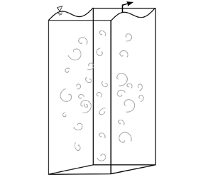
In the present study we aim to use direct numerical simulation (DNS) to investigate the effect of waves on the Reynolds shear stress underneath, specifically the dependence of the Reynolds shear stress on the wave phase. We consider an idealized problem set-up where a monochromatic wave is imposed above an initially isotropic turbulence field (figure 1). This problem was first studied by Teixeira & Belcher (Reference Teixeira and Belcher2002) using the rapid distortion theory (RDT), which predicts that the turbulence statistics vary with the wave phase. The wave-phase dependency of the turbulence has been further investigated by Guo & Shen (Reference Guo and Shen2013, Reference Guo and Shen2014) and Chen et al. (Reference Chen, Wan, Wang and Chen2019) using DNS. Guo & Shen (Reference Guo and Shen2014) found that their simulation result can support the RDT prediction of the wave-phase variation of the Reynolds normal stresses. In addition, they identified the processes responsible for these variations through the analyses of the budget of the Reynolds normal stresses. Chen et al. (Reference Chen, Wan, Wang and Chen2019) investigated and quantified the subgrid-scale properties of the turbulence at different wave phases for large-eddy simulation of wave–turbulence interaction. Despite the substantial knowledge about the wave effect on turbulence obtained from these studies, the mechanisms underlying the wave-phase variation of the Reynolds shear stress were not addressed. Considering the importance of Reynolds shear stress in the turbulence transport of momentum and the production of turbulent kinetic energy (Guo & Shen Reference Guo and Shen2014; Skyllingstad & Denbo Reference Skyllingstad and Denbo1995), there is a critical need for its study, which is presented in this paper.

Figure 1. Sketch of the simulation set-up. The axis on the right illustrates the vertical variation of the coefficient of the body force  $\beta$ (2.3). The wave propagates in the $+x$–direction.
We note that the present canonical problem depicted in figure 1 is intended for studying the fundamental mechanisms of wave–turbulence interaction (Teixeira & Belcher Reference Teixeira and Belcher2002). To focus on the wave effect on turbulence, the wave is dynamically maintained (Guo & Shen Reference Guo and Shen2009) and the feedback effect of the turbulence on the wave evolution is suppressed, such that we can obtain accurate turbulence statistics for different wave phases using time averaging for a long duration without the wave getting dissipated or distorted (for detailed discussions, see Guo & Shen Reference Guo and Shen2013). Under realistic ocean conditions, in addition to the non-breaking waves, the air–sea interface involves more complex processes, including wind shear, Coriolis force, wave breaking, spray and bubbles. The turbulence in the upper ocean can also be affected by motions at larger scales, such as the internal waves and fronts. In the present set-up, absent of other types of forcing, it is ensured that turbulence is affected by the wave only. Moreover, the isotropic turbulence is fundamental to the understandings of many turbulence dynamics. Turbulence at small scales can be considered to be reasonably isotropic and, therefore, the study of isotropic turbulence is crucial to the development of turbulence theories (Tennekes & Lumley Reference Tennekes and Lumley1972; Sreenivasan & Antonia Reference Sreenivasan and Antonia1997; Pope Reference Pope2000; Ishihara, Gotoh & Kaneda Reference Ishihara, Gotoh and Kaneda2009). Some realistic flows may also be approximated by the isotropic turbulence. For example, the turbulence injected by breaking waves can be considered nearly isotropic (Rapp & Melville Reference Rapp and Melville1990; Isler et al. Reference Isler, Fritts, Andreassen and Wasberg1994; Gemmrich & Farmer Reference Gemmrich and Farmer2004) so the subsequent modifications of the turbulence by the waves arriving later may be investigated by the present canonical model for the first step of study. The canonical set-up of isotropic turbulence was also adopted in previous theoretical studies (e.g. Teixeira & Belcher Reference Teixeira and Belcher2000) and experimental studies (e.g. Variano & Cowen Reference Variano and Cowen2013) of the turbulence near a shear-free boundary.
This study also seeks to understand the effect of the curved surface of waves on turbulence. To resolve the wave-phase dependence of the turbulent flows, it is no longer appropriate to treat the surface as a rigid and flat lid as in the wave-phase-averaged model. The effects of boundary curvature have been studied extensively for boundary layers over stationary curved walls (see e.g. Bradshaw Reference Bradshaw1969; So & Mellor Reference So and Mellor1973; Hoffmann, Muck & Bradshaw Reference Hoffmann, Muck and Bradshaw1985; Moser & Moin Reference Moser and Moin1987; Zeman & Jensen Reference Zeman and Jensen1987; Baskaran, Smits & Joubert Reference Baskaran, Smits and Joubert1991; Hall & Horseman Reference Hall and Horseman1991; Holloway & Tavoularis Reference Holloway and Tavoularis1992; Neves & Moin Reference Neves and Moin1994). The extra strain rates, which may arise from the curved flow direction and the converge or diverge of the flow, can have a significant effect on the turbulence in addition to the simple shear  $\partial U/\partial y$ (Bradshaw Reference Bradshaw1973). Specifically for the curvature effect, it is found that a concave wall destabilizes the turbulence and enhances the Reynolds shear stress whereas a convex wall has an opposite effect on the turbulence (So & Mellor Reference So and Mellor1973; Moser & Moin Reference Moser and Moin1987). The Taylor–Götler vortices that arise from the centrifugal instability are also associated with the curvature effect (Saric Reference Saric1994).
In the studies of the airflow in turbulent wind over water waves, the phase dependency of the Reynolds stresses owing to the perturbations of the wave surface has also been observed (see e.g. Belcher & Hunt Reference Belcher and Hunt1993; Belcher, Newley & Hunt Reference Belcher, Newley and Hunt1993; Yang & Shen Reference Yang and Shen2009, Reference Yang and Shen2010; Hara & Sullivan Reference Hara and Sullivan2015; Buckley & Veron Reference Buckley and Veron2016; Husain et al. Reference Husain, Hara, Buckley, Yousefi, Veron and Sullivan2019; Yousefi, Veron & Buckley Reference Yousefi, Veron and Buckley2020, Reference Yousefi, Veron and Buckley2021). The turbulent stress was found to be asymmetric about the wave crest. For example, experimental (Buckley & Veron Reference Buckley and Veron2016; Yousefi et al. Reference Yousefi, Veron and Buckley2020) and numerical studies (Yang & Shen Reference Yang and Shen2010; Hara & Sullivan Reference Hara and Sullivan2015) found that the turbulent shear stress is reduced on the windward side of the waves and intensified on the leeward side. The turbulent kinetic energy was found to be enhanced downwind of the wave crests above the leeward side (Yousefi et al. Reference Yousefi, Veron and Buckley2021). In particular, Yousefi et al. (Reference Yousefi, Veron and Buckley2021) were able to obtain detailed measurements of the turbulence production and the energy transfer between wave coherent motions and turbulence at different phases. The pressure is also wave-phase dependent and asymmetric about the wave crest, contributing to the form drag (Belcher & Hunt Reference Belcher and Hunt1993; Belcher et al. Reference Belcher, Newley and Hunt1993).
Comparatively, there are fewer studies focusing on the effect of curvature on the turbulence under waves. Lucarelli et al. (Reference Lucarelli, Lugni, Falchi, Felli and Brocchini2018) found that during the evolution of a spilling breaker, the extra strain rate induced by the highly curved surface can have comparable influence with the shear straining on the Reynolds shear stress in a near-surface turbulent shear layer. The dynamics of vorticity and turbulent kinetic energy were also found to be related to the curvature and rotation of this shear layer (Lucarelli et al. Reference Lucarelli, Lugni, Falchi, Felli and Brocchini2019). For the non-breaking waves, the curvature of the wave surface is milder and periodically varies with the wave phase. It would be desired to understand whether it can influence the water turbulence.
The analyses of flows with a curved boundary are often made easier when evaluating the governing equations of motions in curvilinear coordinates. Different curvilinear coordinates have been employed in previous studies. One of the choices is the  $(s,n)$ coordinates (Bradshaw Reference Bradshaw1973; Castro & Bradshaw Reference Castro and Bradshaw1976; Baskaran et al. Reference Baskaran, Smits and Joubert1991). The $s$-coordinate lines reference a single selected curve, usually a boundary or a streamline, and the $n$-coordinate lines are orthogonal to the $s$ lines. Lucarelli et al. (Reference Lucarelli, Lugni, Falchi, Felli and Brocchini2018, Reference Lucarelli, Lugni, Falchi, Felli and Brocchini2019) successfully applied the $(s,n)$ coordinate frame to the study of the spilling breakers and examined the role of the extra strain rates associated with the curvature in the turbulence dynamics. However, except for simple parallel rotating flows, there exists a mean velocity component in the $n$-direction, which may introduce some complexities for flows with varying curvature. There are also other generalized curvilinear coordinates that are explicitly defined based on the boundary geometry. These coordinate systems share some features with the $(s,n)$ coordinates in that the cross-flows may be present but the coordinate transformation is easy to define. For example, the boundary conforming non-orthogonal coordinates that only map the vertical coordinate have been used for various studies of turbulent flows over progressive waves (Hsu, Hsu & Street Reference Hsu, Hsu and Street1981; Sullivan et al. Reference Sullivan, Edson, Hristov and McWilliams2008; Yang & Shen Reference Yang and Shen2009, Reference Yang and Shen2010; Hara & Sullivan Reference Hara and Sullivan2015; Yang & Shen Reference Yang and Shen2017; Hao & Shen Reference Hao and Shen2019) and turbulence under water waves (Guo & Shen Reference Guo and Shen2013, Reference Guo and Shen2014; Xuan & Shen Reference Xuan and Shen2019; Xuan et al. Reference Xuan, Deng and Shen2019). Boundary conforming orthogonal coordinate mapping with decaying curvature away from the surface proposed by Benjamin (Reference Benjamin1959) has also been employed to investigate the wave effect on the turbulent wind (Belcher & Hunt Reference Belcher and Hunt1993; Sullivan, McWilliams & Moeng Reference Sullivan, McWilliams and Moeng2000; Buckley & Veron Reference Buckley and Veron2016; Yousefi & Veron Reference Yousefi and Veron2020; Yousefi et al. Reference Yousefi, Veron and Buckley2020, Reference Yousefi, Veron and Buckley2021). In particular, Yousefi & Veron (Reference Yousefi and Veron2020) derived the governing equations with triple decomposition for the turbulent airflow over waves in the orthogonal curvilinear coordinates and applied those to the analyses of the balance of momentum and kinetic energy (Yousefi et al. Reference Yousefi, Veron and Buckley2020, Reference Yousefi, Veron and Buckley2021). They found for the first time that some quantities, such as the wave-induced and turbulent shear stresses, can be drastically different when evaluated under the curvilinear coordinates compared with under Cartesian coordinates. Their analyses indicate that a proper choice of coordinate frame can help the evaluation of flow statistics at the boundary and provide insightful interpretation of the flow dynamics of the air–wave interactions.
The streamline coordinates, which use the mean streamlines as coordinate lines, ensure that the mean velocity is aligned with the coordinate axes everywhere. For a two-dimensional irrotational flow, the equipotential lines and streamlines form an orthogonal coordinate system. Finnigan (Reference Finnigan1983) developed the streamline coordinates for generalized two-dimensional shear flows, which have been used for a variety of problems, such as flows over hills (Finnigan Reference Finnigan2004; Poggi & Katul Reference Poggi and Katul2007; Li, Zimmerman & Princevac Reference Li, Zimmerman and Princevac2008) and wake flows behind a barrier (Finnigan & Bradley Reference Finnigan and Bradley1983). Although streamline coordinates can be laborious to define, they are sometimes desired because some analyses are substantially simplified when the equations of motions are expressed in streamline coordinates, e.g. the equations of the RDT describing the flow over bluff bodies (Durbin & Hunt Reference Durbin and Hunt1980).
In the present paper, the wave-following streamline coordinates are used to analyse the wave motions and Reynolds shear stress for the canonical problem sketched in figure 1. We find that the streamline coordinates are superior to the Cartesian coordinates for the analyses of the Reynolds shear stress because the former gives a more accurate definition of the Reynolds shear stress as the momentum flux between the surface region and the deep region in the wave flows. By comparison, the definition of the Reynolds shear stress in the Cartesian coordinate system is affected by the pseudo stress generated from the kinematic effect of the wave surface. In addition, we discover that the streamline curvature of the wave plays an important dynamical role in the wave-phase variation of the Reynolds shear stress. The production of the Reynolds shear stress near the water surface is mostly owing to the curvature effect, based on which we propose a scaling law quantifying the wave-phase variation of the Reynolds shear stress. Moreover, the modelling of the pressure–strain correlation is explored by combining classic models with a correction accounting for the curvature effect. The new model, which can capture the main features of the DNS results, not only shows that the curvature effect is important, but also demonstrates the possibility of modelling the wave effect utilizing the curvature information.
The present study intends to extend the knowledge about the effect of non-breaking waves on the initially isotropic turbulence obtained in Guo & Shen (Reference Guo and Shen2013, Reference Guo and Shen2014) by addressing the lack of understanding about the Reynolds shear stress. This can help gain more insights into the role of non-breaking waves in the turbulent momentum transport and turbulent kinetic energy production, both of which are related to the Reynolds shear stress. Previously, it was found that the cumulative tilting of turbulence vertical vortices by waves towards the streamwise direction is connected to the generation of the mean Reynolds shear stress in the initially isotropic turbulence (Guo & Shen Reference Guo and Shen2013). Guo & Shen (Reference Guo and Shen2014) found that the energy transfer from the wave to turbulence is related to the phase correlation between the Reynolds shear stress and the wave straining. Despite its importance, the dynamics of Reynolds shear stress in the flow were elusive in Guo & Shen (Reference Guo and Shen2013, Reference Guo and Shen2014). The present study provides an accurate definition and description of the Reynolds shear stress, elucidates its underlying dynamics, and presents a new method for modelling the wave–turbulence interaction. Furthermore, the previous works used the Cartesian coordinates whereas the present work uses the wave-following streamline coordinates, which provides a different perspective of wave–turbulence interactions in general. However, we shall note that not all turbulence statistics are sensitive to the choice of coordinate frame. For example, the Reynolds normal stresses are only slightly affected when transformed from Cartesian coordinates to the streamline coordinates. Considering that the Reynolds normal stresses have already been investigated in depth by Guo & Shen (Reference Guo and Shen2014), we mainly focus on the effect of the coordinate frame on the Reynolds shear stress and its physical interpretation in the present paper.
The remainder of the paper is organised as follows. In § 2 the simulation set-up and computational parameters are introduced. In § 3 the results of the Reynolds shear stress defined under the Cartesian coordinates are discussed. Then in § 4 the analyses using the wave-following streamline coordinates, including the wave-phase variation of the Reynolds shear stress and its budget equation, are presented. The curvature effect on the production of Reynolds shear stress and modelling of pressure–strain correlation are also discussed in this section. In § 5 conclusions are summarised.
2. Computational set-up and parameters
As illustrated in figure 1, the computational domain is a rectangular box with a progressive surface wave at the top. The Cartesian coordinates,  $(x, y, z)$, refer to the streamwise, vertical and spanwise directions, respectively. The wave propagates in the $+x$–direction. The $x$ and $z$ directions are periodic, and the origin of the $y$ coordinate $y=0$ is set at the mean water level. The governing equations for the simulated flow are
 $$\begin{gather} \frac{\partial{\boldsymbol{u}}}{\partial{t}} + \boldsymbol{\nabla}\boldsymbol{\cdot}({\boldsymbol{u}\boldsymbol{u}}) ={-}\frac{1}{\rho}\boldsymbol{\nabla} p + \nu \nabla^{2} \boldsymbol{u} + \boldsymbol{f}, \end{gather}$$
 $$\begin{gather}\boldsymbol{\nabla}\boldsymbol{\cdot} \boldsymbol{u} = 0, \end{gather}$$
where  $\boldsymbol {u}$ denotes the velocity; the velocity components in the $x, y$ and $z$ directions in Cartesian coordinates are denoted by $u, v$ and $w$, respectively; $p=P+\rho gz$ is the dynamic pressure that removes the hydrostatic part from the total pressure $P$, where $\rho$ is the density and $g$ is the gravitational acceleration; $\nu$ is the kinematic viscosity; $\boldsymbol {f}$ is a turbulent body force that energizes the isotropic turbulence. We use a linear forcing method (Lundgren Reference Lundgren2003; Rosales & Meneveau Reference Rosales and Meneveau2005) for the turbulence forcing term, given as
 \begin{equation} \boldsymbol{f} = \beta \boldsymbol{u}'.\end{equation}
Here,  $\beta$ is the parameter controlling the forcing strength and $\boldsymbol {u}'$ is the velocity fluctuations with respect to the $x$-
$x$- $y$ plane-averaged velocity. The balance between the energy input by the forcing term and the dissipation yields $\beta ^{-1}\sim q/\epsilon$, with $q$ being the turbulent kinetic energy and $\epsilon$ being the rate of dissipation. Note that $\beta ^{-1}$ has a dimension of time and determines a turnover time of the turbulence (Rosales & Meneveau Reference Rosales and Meneveau2005). To prevent the linear forcing from interfering with the wave forcing, its strength changes in the vertical direction as shown in the right half of figure 1. The coefficient $\beta$ is a constant $\beta =\beta _0$ in the bulk region, which occupies the centre of the simulation domain, $|{y-y_c}| \leq H_{{b}}$ with $y_c$ being the $y$ coordinate of the centre and $H_{{b}}$ being the half-height of the bulk region. Outside of the bulk region, $\beta$ gradually decays to $0$ over a height of $H_{d}$ as
 \begin{equation} \beta = \frac{\beta_0}{2}\left[{1-\cos \left(\frac{{\rm \pi}(|y-y_c|-H_{{b}}-H_{{d}})}{H_{d}}\right)} \right], \quad H_{{b}} < |y-y_c| \leq H_{{b}}+H_{{d}}. \end{equation}
The region with decaying  $\beta$ is referred to as the damping region. The free region, whose height is $H_{f}$, has no turbulence body force. The turbulence generated in the bulk region and damping region interacts with the surface wave in the free region near the surface. The imposed monochromatic surface wave is dynamically maintained by a pressure forcing method (Guo & Shen Reference Guo and Shen2009) such that the amplitude and shape of the progressive wave are kept statistically steady to yield converged turbulence statistics underneath after performing time averaging. No tangential shear stress is applied on the free surface. The free-slip boundary condition is also imposed at the bottom.
The evolution of the surface elevation  $\eta (x,z,t)$ and the stress balance across the surface are governed by the free-surface kinematic and dynamic boundary conditions, respectively. The free-surface flow simulations are conducted on a wave-boundary-fitted computational grid (Yang & Shen Reference Yang and Shen2011; Guo & Shen Reference Guo and Shen2013; Xuan & Shen Reference Xuan and Shen2019), on which (2.1) and (2.2) are transformed into the computational coordinates and solved. The horizontal derivatives are calculated using the Fourier pseudo-spectral method and the vertical derivatives are calculated using the finite-difference scheme. The fractional-step method is used to advance the momentum equations (2.1) in time subject to the incompressibility condition (2.2). The above numerical method has been tested extensively by Guo & Shen (Reference Guo and Shen2009) and Yang & Shen (Reference Yang and Shen2011) and has been found effective in capturing the dynamics of turbulence interacting with surface waves (Guo & Shen Reference Guo and Shen2013, Reference Guo and Shen2014; Chen et al. Reference Chen, Wan, Wang and Chen2019; Xuan et al. Reference Xuan, Deng and Shen2019, Reference Xuan, Deng and Shen2020).
The simulations are performed using dimensionless quantities. The characteristic length scale  $L$ is set to $1/2{\rm \pi}$ of the streamwise domain size, i.e. the dimensionless streamwise size $L_x$ is $2{\rm \pi}$. The characteristic time scale $T$ for the non-dimensionalization is chosen such that the dimensionless $\beta _0$ is $0.1$ (note that the coefficient in the forcing term (2.3) is associated with a turnover time scale as introduced above). Hereafter, the variables are all non-dimensionalized by $L$ and $T$ unless specified otherwise. The parameters for the cases considered in this study are listed in table 1. In all cases, the wavelength of the surface wave is fixed to $\lambda =2{\rm \pi}$, i.e. the wavenumber $k$ is set to $1$. The steepness $ak$ and angular frequencies $\sigma$ of the wave are varied in different cases, resulting in different strain rates of the wave orbital motions $S=ak\sigma$. The wave in case I has a steepness $ak=0.1$ with a characteristic strain rate $S = 1$. Case II is simulated with a larger steepness $ak=0.15$ but has the same strain rate as case I to show the effect of the wave slope on the turbulence dynamics. Because the wave straining rate also relates to the turbulence dynamics, case III is set up based on case II but with an increased straining rate $S=1.5$. The above choices of $ak$ and $S$ values were shown representative for wave–turbulence interaction studies (Guo & Shen Reference Guo and Shen2013).
Table 1. Non-dimensional computational parameters for waves and turbulence in the present study. These parameters are non-dimensionalized by the characteristic length scale  $L, 1/{\rm \pi}$ of the streamwise domain size, and the characteristic time scale $T$, which scales the forcing coefficient $\beta _0$ to $0.1$ (the forcing coefficient is associated with the turnover time scale of the isotropic turbulence generated).

Referring to figure 1, the dimensions of the domain are  $L_x \times \bar {H} \times L_z = 2{\rm \pi} \times 5{\rm \pi} \times 2{\rm \pi}$ with $\bar {H}$ being the mean water depth. The heights of the bulk region, damping region and free region are $3{\rm \pi}, {\rm \pi}/2$ and ${\rm \pi} /2$, respectively. The grid size is $N_x \times N_y \times N_z=256\times 660\times 256$. The grid spacings in the horizontal directions are $\varDelta _x = \varDelta _z = 0.0245$. The vertical grid, which is condensed near the surface, has a maximum grid spacing of $\varDelta _{y}|_{max}=0.0245$ in the bulk region and a minimum spacing of $\varDelta _{y}|_{min}=8.74\times 10^{-4}$ at the surface. The above grid spacings allow a resolution of $\varDelta _x/\eta _K \approx 1.69$, where $\eta _K=(\nu ^{3}/\epsilon )^{1/4}$ is the Kolmogorov scale. This resolution, being smaller than $2$, is considered adequate for resolving most of the small-scale turbulent motions in DNS (Pope Reference Pope2000; Donzis, Yeung & Sreenivasan Reference Donzis, Yeung and Sreenivasan2008).
The simulations are first run without the imposed surface wave. When the turbulent flow reaches the quasi-equilibrium state, the turbulence statistics are evaluated at the centre of the free region,  $y^{cf}=-{\rm \pi} /4$. They are used as the reference properties of the turbulence near the free surface without the distortion of the wave straining for cases I–III. At $y=y^{cf}$, the root mean square of the turbulence velocity fluctuations $u^{rms,cf}$ is $0.115$ and the Taylor microscale $\lambda _g^{cf}$ is $0.235$. The Reynolds number based on the Taylor scale, defined as $Re_{\lambda }^{cf}=u^{rms,cf}\lambda _g^{cf}/\nu$, is $68$. The Kolmogorov scale $\eta _K$ is $0.0145$. The integral length scale defined as $L_\infty ^{cf}=u^{rms,cf}{(\lambda _g^{cf})}^{2}/15\nu$ is $1.06$. The isotropy of the generated turbulence is validated in Guo & Shen (Reference Guo and Shen2009). After the turbulence is fully developed, the wave is added to the simulation using the pressure forcing method of Guo & Shen (Reference Guo and Shen2009) and the statistics are collected after the simulation reaches the statistically steady state again. To ensure that the conclusions are not affected by the uncertainties of the numerical results, we calculated the uncertainties of the key statistics of interest using the method described by Oliver et al. (Reference Oliver, Malaya, Ulerich and Moser2014), which gives an accurate estimation of the sampling error by using an autoregressive model to account for the correlations in the sampled quantities from DNS. For Reynolds normal stresses and shear stress, the estimated standard deviation is less than 5.5 % in the free region (figure 1). Although the discretization error is also a source of the uncertainty, the study by Mohan, Fitzsimmons & Moser (Reference Mohan, Fitzsimmons and Moser2017) indicates that the usual criteria for the grid resolution for DNS of the homogeneous isotropic turbulence, which are satisfied in the present study as described above, can ensure that the discretization error of the turbulent kinetic energy is negligible. Therefore, the uncertainties owing to the discretization error should not affect our analyses.
3. Reynolds shear stress in Cartesian coordinates
In this section we examine the distribution of Reynolds shear stress defined under Cartesian coordinates. We first define the mean velocity  $\langle {\boldsymbol {u}}\rangle (x,y)$, which is obtained from the averaging with respect to specific wave phases as
 \begin{equation} \langle{\boldsymbol{u}}\rangle(x, y) = \frac{1}{T_s}\frac{1}{L_z}\int_{T_s}\int_{L_z} \boldsymbol{u}(x+ct, y, z, t) \,\mathrm{d}z\,\mathrm{d}t, \end{equation}
where  $T_s$ is the averaging period and $c=\sigma /k$ is the wave phase speed. The mean velocity defined above corresponds to the wave motions. The turbulent fluctuation is defined as
 \begin{equation} \boldsymbol{u'}(x, y, z, t) = \boldsymbol{u} - \langle{\boldsymbol{u}}\rangle. \end{equation}
 The Reynolds shear stress,  $\langle {-u'v'}\rangle$, is shown in figure 2. We can see that the interaction of the turbulence with the wave induces a pronounced variation of $\langle {-u'v'}\rangle$ with the wave phase. For all the cases considered in this work, strong Reynolds shear stress exists mainly in three regions. The first region with large values of $\langle {-u'v'}\rangle$ is under the backward slope near the wave crest. This region extends from the deep region and gradually decreases towards the water surface. In addition, we can see two regions with high $\langle {-u'v'}\rangle$ located under the surface and roughly symmetrically about the wave trough. The values of $\langle {-u'v'}\rangle$ in these two regions have opposite signs, i.e. positive under the forward slope side of the wave and negative under the backward slope side, respectively. We also note that the magnitudes of $\langle {-u'v'}\rangle$ in these two regions increase towards the surface, in contrast to the behaviour of $\langle {-u'v'}\rangle$ in the first region. This difference indicates that the correlations between $u'$ and $v'$ in the above regions are governed by different mechanisms.

Figure 2. Contours of the normalized Reynolds shear stress  $-\langle {u'v'}\rangle /{(u^{rms,cf})}^{2}$ defined in Cartesian coordinates for (a) case I ( $ak=0.1, Fr=0.1$), (b) case II ( $ak=0.15, Fr=0.15$) and (c) case III ( $ak=0.15, Fr=0.1$). The increment of contours is 0.015. Note that the horizontal and vertical coordinates are plotted on different scales.
To further understand the Reynolds shear stress, we use the joint probability density function (JPDF) to quantify the correlations between  $u'$ and $v'$ and analyse the turbulent motions associated with the Reynolds shear stress. As an example, figure 3 plots the contours of the JPDF under different wave phases near the surface for case I at a fixed distance from the surface, $k(y-\eta ) = -0.01$. According to which quadrant the velocity fluctuations are located, the turbulent motions are classified into four categories: Q1 ( $u'>0, v'>0$); Q2 ( $u'<0, v'>0$); Q3 ( $u'<0, v'<0$); Q4 ( $u'>0, v'<0$) (Wallace, Eckelmann & Brodkey Reference Wallace, Eckelmann and Brodkey1972). The elliptically shaped contours of JPDF indicate that the magnitude of $v'$ is smaller than that of $u'$, which is due to the suppression of the vertical fluctuations near the surface. We find that the major axes of the JPDF contours are roughly aligned with the wave surface under the backward slope (figure 3a) and the forward slope (figure 3c) (the local slope is indicated by the dash–dotted line). This phenomenon indicates that the velocity fluctuations near the surface tend to be parallel to the local wave surface, i.e.
 \begin{equation} \frac{v'}{u'} \approx \eta_x. \end{equation}
As a result, under the forward slope ( $\eta _x < 0$), Q2 and Q4 motions are dominant, resulting in positive $\langle {-u'v'}\rangle$ (figure 2). The negative $\langle {-u'v'}\rangle$ under the backward slope ( $\eta _x>0$) results from the dominance of the Q1 and Q3 events. The above correlation between $u'$ and $v'$ can be explained by the blockage effect imposed by the free-surface boundary conditions, which restrict the motions normal to the boundary and transfers kinetic energy from the surface-normal fluctuations to surface-parallel motions (Perot & Moin Reference Perot and Moin1995; Walker, Leighton & Garza-Rios Reference Walker, Leighton and Garza-Rios1996; Shen et al. Reference Shen, Zhang, Yue and Triantafyllou1999; Guo & Shen Reference Guo and Shen2010). Here, because the wave surface is inclined, the constraint imposed by the boundary, i.e. $\boldsymbol {u'}\boldsymbol {\cdot } \boldsymbol {n}=0$, reduces to the correlation given in (3.3), which leads to the two roughly symmetric regions of $\langle {-u'v'}\rangle$ with opposite signs shown in figure 2. As the surface is approached and the blockage effect becomes stronger, the correlation between $u'$ and $v'$ grows and, thus, the strength of $\langle {-u'v'}\rangle$ in these two regions increases towards the surface (figure 2). Meanwhile, the energy transferred from surface-normal fluctuations to surface-parallel fluctuations further contributes to the enhancement of $\langle {-u'v'}\rangle$.

Figure 3. Joint probability density function of  $u'$ and $v'$ for case I under the (a) backward slope, (b) crest, (c) forward slope and (d) trough of the wave at $k(y-\eta )=-0.01$. The wave slopes under the backward and forward slopes are indicated using dash–dotted lines in (a) and (c). Note that the axes are stretched to highlight the orientations of the contours. The smallest (outermost) contour level is $0.02$ and the increment between contours is $0.06$. The velocity fluctuations are normalized by $u^{rms,cf}$.
Similar distribution of the Reynolds shear stress  $\langle {-u'v'}\rangle$ caused by the blockage effect has also been observed in other types of flows. For example, for the spilling breaking waves, it was found that the Reynolds shear stress is positive at the front of the crest and negative at the lee side within the turbulent shear layer induced by the breaker (figure 2 in Lucarelli et al. Reference Lucarelli, Lugni, Falchi, Felli and Brocchini2018). In the turbulent wind boundary layer over water waves, various studies have also observed the negative–positive turbulent shear stress along the wave crest (Yang & Shen Reference Yang and Shen2010; Buckley & Veron Reference Buckley and Veron2016; Husain et al. Reference Husain, Hara, Buckley, Yousefi, Veron and Sullivan2019), which is also attributed to the flow aligning with the sloped wave surface by Yousefi et al. (Reference Yousefi, Veron and Buckley2020) after they compared the results under different coordinate frames.
However, we shall note that the  $\langle {-u'v'}\rangle$ induced by the wave surface boundary conditions has a different meaning in terms of the momentum transport compared with the Reynolds shear stress in flows over a flat boundary. In the turbulent boundary layer over a flat boundary, the Reynolds shear stress represents the exchange of momentum in the direction normal to the boundary. However, in a wave flow, the mean velocity direction changes with the wave phase, leading to the rise and fall of the fluid elements. In this scenario, the kinematic-induced $\langle {-u'v'}\rangle$ is a pseudo Reynolds shear stress that just represents motions that are along the free surface and is not fully representative of the momentum exchange between the deep and near-surface regions in the wave flow. Therefore, a more accurate representation of the Reynolds shear stress is called for.
As shown in figure 2, the influence of the boundary conditions seems to extend down to approximately  $k(y-\eta )=-0.1$ below the surface, where the two regions with strong $\langle {-u'v'}\rangle$ around the wave trough disappear. Meanwhile, the region under the backward slope still has large values of $\langle {-u'v'}\rangle$, indicating that there may exists an enhanced momentum transport under the backward slope. However, with the contributions from the pseudo Reynolds shear stress due to the kinematic constraint unquantified, it is difficult to determine the ‘real’ momentum transport. To remedy this bias induced by the kinematic effect in the interpretation of the Reynolds shear stress, the direction of the mean flow is taken into consideration in § 4 using the wave-following streamline coordinates. Yousefi et al. (Reference Yousefi, Veron and Buckley2020) reached a similar conclusion for the turbulent wind flow over waves, i.e. the turbulent shear stress evaluated under a curvilinear coordinate system accounts for the effect of the inclined surface directly. The Reynolds shear stress near and away from the surface are analysed in the streamline coordinates in the sections below.
4. Analyses under wave-following streamline coordinates
In this section we introduce the streamline coordinates that account for the varying mean flow direction to address the issue pointed out in § 3 that the  $\langle {-u'v'}\rangle$ in Cartesian coordinates does not faithfully quantify the momentum transport in a wavy domain. The definition of the streamline coordinates is given in § 4.1. Then, the properties of the wave motions viewed in the streamline coordinates are discussed in § 4.2. The Reynolds shear stress in the wave-following frame and its budget are examined in § 4.3. Details about the curvature effect on the production of Reynolds shear stress and the pressure–strain correlation are discussed in § 4.4.
4.1. Definition of wave-following streamline coordinates
To facilitate the definition of the streamline coordinates, the flow is translated to the wave-following frame such that the mean flow, i.e. the wave motions, becomes a quasi-steady, two-dimensional flow in the  $x$–
$x$– $y$ plane. The translated mean velocity field $(\langle {u}\rangle -c, \langle {v}\rangle )$ is plotted in figure 4(a) using vector arrows, which show that the flow direction is opposite to the direction of wave propagation. Following Finnigan (Reference Finnigan1983), for the two-dimensional steady mean flow that depends on $x$ and $y$, the transformation from the Cartesian coordinates $(x, y, z)$ to the streamline coordinates $(\xi _1,\xi _2,\xi _3)$ is performed only for the first two dimensions and does not affect the transverse direction $z$ or $\xi _3$, i.e. $z=\xi _3$. The coordinate lines of $\xi _1$ and $\xi _2$ are defined as the streamlines and the lines that are orthogonal to the streamlines, respectively. The streamlines are given by the lines of $\psi (x,y)=\text {constant}$, where $\psi (x,y)$ is the streamfunction defined by the relations
 \begin{equation} \frac{\partial{\psi}}{\partial{y}} = \langle{u}\rangle - c, \quad \frac{\partial{\psi}}{\partial{x}} ={-}\langle{v}\rangle. \end{equation}
The other group of coordinate lines is given by the function  $\phi (x, y)$, defined as
 \begin{equation} \frac{\partial{\phi}}{\partial{x}} = \zeta (\langle{u}\rangle - c), \quad \frac{\partial{\phi}}{\partial{y}} = \zeta \langle{v}\rangle. \end{equation}
Note that the lines of  $\phi (x,y)=\text {constant}$ are orthogonal to the streamlines. The parameter $\zeta$ in the above definition is calculated using
 \begin{equation} \zeta = \exp\left(\int \frac{\varOmega}{U^{2}} \,\mathrm{d}\psi\right),\end{equation}
where  $U=|(\langle {u}\rangle -c,\langle {v}\rangle )|$ is the mean velocity magnitude and $\varOmega = \partial \langle {v}\rangle /\partial x - \partial \langle {u}\rangle /\partial y$ is the vorticity of the mean flow. We remark that when the flow is irrotational, the parameter $\zeta$ calculated from (4.3) is simply $\zeta =1$, and the function $\phi (x,y)$, (4.2a,b), reduces to the velocity potential, i.e. $\boldsymbol {\nabla } \phi = (\langle {u}\rangle -c, \langle {v}\rangle )$. Although $\phi$ and $\psi$ can be directly used as the coordinates of an orthogonal coordinate system, the magnitudes of the base vectors of the $(\phi,\psi )$ system vary from place to place with respect to the Cartesian frame, in addition to the difference in dimensions, which makes it difficult to measure quantities using these coordinates and compare them with those measured under Cartesian coordinates. Therefore, we further normalize the basis vectors by their local magnitudes and the resulting coordinates $\xi _1$ and $\xi _2$ satisfy
 \begin{equation} \mathrm{d}\xi_1= {(\zeta U )}^{{-}1} \mathrm{d}\phi, \quad \mathrm{d}\xi_2=U^{{-}1} \mathrm{d}\psi. \end{equation}
In this way, the quantities in the streamline coordinates  $(\xi _1,\xi _2,\xi _3)$ defined above are properly scaled and have the same physical dimensions as the Cartesian coordinates.

Figure 4. (a) The mean velocity vectors  $(\langle {u}\rangle -c, \langle {v}\rangle )$ and contours of the mean velocity magnitude ${U}=|(\langle {u}\rangle -c, \langle {v}\rangle )|$. Note that the along-stream component of the mean velocity in streamline coordinates satisfies $\hat {U}=U$. (b) The $\xi _1$ and $\xi _2$ coordinate lines of the streamline coordinates.
A  $\xi _1$– $\xi _2$ plane of the wave-following streamline coordinates is plotted schematically in figure 4(b). The wave surface, as a material boundary, is a streamline in the wave-following frame. The other streamlines ( $\xi _2=\text {constant}$) are roughly parallel to the wave surface, with decreasing curvature as the distance from the surface increases. This is expected because the wave motions decay with the depth and the streamlines should become straight in deep waters with the influence of the wave diminishing. We note that the directions of the axes of the above streamline coordinates are different from those of Cartesian coordinates. The along-stream coordinate $\xi _1$ increases in the $-x$-direction, consistent with the mean flow direction shown in figure 4(a). The positive direction of the cross-stream coordinate $\xi _2$ roughly points downward to the interior of the flow and the right-hand system is maintained.
4.2. Mean flow properties
In this section we discuss properties of the wave using the wave-following streamline coordinate system for the subsequent analyses of the wave–turbulence interaction. For more intuitive interpretation of the figures, hereafter, the results are plotted in the physical domain using Cartesian coordinates  $(x, y, z)$ but the dependent variables, such as the velocity, are defined based on the streamline coordinates. The values evaluated in streamline coordinates are denoted by $\widehat {(\cdot )}$. For example, the velocity components in the $\xi _1, \xi _2$ and $\xi _3$ directions of the streamline coordinates are denoted by $\hat {u}, \hat {v}$ and $\hat {w}$, respectively.
In the streamline coordinates, the only non-zero component of the mean velocity  $\hat {\boldsymbol {U}}$ is the along-stream component $\hat {U}$, which is equal to the velocity magnitude $U$. The cross-stream mean velocity is zero by definition. The dimensionless mean momentum equation in the $\xi _1$-direction is written as (Finnigan Reference Finnigan1983)
 \begin{align} \frac{\partial \hat{U}}{\partial t} + \hat{U}\frac{\partial \hat{U}}{\partial \xi_1} &={-}\frac{\partial \langle{p}\rangle}{\partial \xi_1} - \frac{\partial \langle{\hat{u}'^{2}}\rangle}{\partial \xi_1} + \frac{\langle{\hat{u}'^{2}}\rangle - \langle{\hat{v}'^{2}}\rangle}{\gamma} - \frac{\partial \langle{\hat{u}'\hat{v}'}\rangle}{\partial \xi_2} + \frac{2 \langle{\hat{u}'\hat{v}'}\rangle}{R} \nonumber\\ &\quad + \frac{1}{Re} \left[\frac{\partial \hat{U}}{\partial \xi_1^{2}} + \frac{\partial \hat{U}}{\partial \xi_2^{2}} - \frac{2}{\gamma}\frac{\partial \hat{U}}{\partial \xi_1} - \frac{1}{R}\frac{\partial \hat{U}}{\partial \xi_2} - \frac{\hat{U}}{R^{2}}\right]. \end{align}
In the above equation,  $\gamma$ and $R$ are two length scales arising naturally from the definitions of the wave-following streamline coordinates and their physical meanings are detailed below.
Figure 4(a) plots the contours of  $\hat {U}$ for case I with $ak=0.1$ and $S=1$ as an example. We can see that the maximum and minimum velocity occurs under the wave trough and crest, respectively. Under the forward slope, the flow slows down along the streamlines, accompanied by the elevation of the water surface. The reverse process, i.e. the flow acceleration, occurs under the backward slope as the surface elevation decreases. Such periodic acceleration and deceleration along the streamlines can be quantified using a length scale $\gamma$ defined as
 \begin{equation} \gamma^{{-}1} = \frac{1}{\hat{U}}\frac{\partial{\hat{U}}}{\partial{\xi_1}} = \frac{\partial{\ln \hat{U}}}{\partial{\xi_1}}.\end{equation}
According to the above definition,  $\gamma$ is the ‘e-folding’ length of the streamwise velocity $\hat {U}$. A larger $\gamma ^{-1}$ indicates that the local relative acceleration rate of the flow is larger. The contours of $\gamma ^{-1}$ are shown in figure 5(a). The negative and positive $\gamma ^{-1}$ under the wave forward and backward slopes correspond to the flow deceleration and acceleration, respectively. This parameter is also associated with the streamwise stretching and compression imposed on the fluid elements by the wave motions. As the flow accelerates, the fluid elements are stretched along the streamline. On the contrary, the deceleration of the flow leads to the effect of streamwise compression. It should be noted that for steady progressive waves, the mean flow does not detach from the wave surface even with the deceleration. In a more violent scenario, such as in a spilling breaker (Dabiri & Gharib Reference Dabiri and Gharib1997) or hydraulic jump (Misra et al. Reference Misra, Kirby, Brocchini, Veron, Thomas and Kambhamettu2008), a sharp deceleration of the mean flow can occur and the associated flow separation can induce intense generation of turbulence vorticity.

Figure 5. Contours of (a)  $\gamma ^{-1}$ and (b) $R^{-1}$ for case I. The values are normalized by $ak^{2}$. The yellow line with arrows represents a streamline and the direction of the mean flow.
Another important parameter introduced by the streamline coordinate system is the local curvature of the streamlines,  $R^{-1}$, defined using the mean vorticity $\varOmega$ and streamwise velocity $\hat {U}$ as
 \begin{equation} R^{{-}1} = \frac{1}{\hat{U}}\left(\varOmega + \frac{\partial{\hat{U}}}{\partial{\xi_2}}\right).\end{equation}
It can be shown that the definition above is equivalent to the geometric curvature of the streamline (or the coordinate lines of  $\xi _1$), for which the details are given in Appendix A. The contours of the streamline curvature for case I are plotted in figure 5(b). The figure shows that the maximum and minimum curvatures occur under the wave crest and trough, respectively. In our definition (4.7), $R^{-1}$ is positive when the centre of the curvature lies in the $+\xi _2$-direction. Therefore, the concave streamlines under the wave crest have positive curvature values whereas the convex flow under the trough has negative curvatures. We note that the flow curvature is associated with the centripetal acceleration of the flow and can be used to quantify the straining effect on the fluid elements caused by the rotation of the mean flow. This is important to the wave-phase variation of the Reynolds shear stress as discussed in the subsequent sections.
Both the acceleration length scale  $\gamma$ and the curvature $R^{-1}$ can be estimated using the linear irrotational wave theory as detailed in Appendix B. The results (B10) and (B11) are written below,
 $$\begin{gather} \gamma^{{-}1} = a k^{2} \, \textrm{e}^{ky} \cos {kx} + O(a^{2} k^{2}), \end{gather}$$
 $$\begin{gather}R^{{-}1} = a k^{2} \, \textrm{e}^{ky} \sin {kx} + O(a^{2} k^{2}). \end{gather}$$
As discussed below, the viscous wave considered in the present study is not perfectly irrotational but the rotational region is confined to a thin viscous layer below the surface. Therefore, the use of the irrotational wave theory can be justified for most of the region away from the surface. Nonetheless, we find that  $\gamma ^{-1}$ and $R^{-1}$ can still be accurately estimated even in the viscous layer using the irrotational wave velocity because the viscous effect does not significantly affect the along-stream acceleration nor the geometry of the streamlines. The numerical results of $\gamma ^{-1}$ and $R^{-1}$ (figure 5) are consistent with the above theoretical estimates (not plotted). Both quantities vary sinusoidally with the wave phase and the magnitudes of their variations scales with $a k^{2}$ and decays exponentially with the depth. This indicates that these two quantities are correlated for the wave orbital motions. However, it should be noted that they are associated with different mechanisms, i.e. streamwise acceleration for $\gamma$ and centripetal acceleration for $R$ but with a phase difference of ${\rm \pi} /2$. As a result, they appear in different budget terms in the transport equation of the Reynolds shear stress, as shown below in § 4.4. If we assume that the characteristic length scale of the energy-containing eddies is the integral length scale $L_\infty ^{cf}$, we can define a relative curvature as $L_\infty ^{cf}/R$. The relative curvature, representative of the curvature effect on the turbulence (Moser & Moin Reference Moser and Moin1987; Baskaran et al. Reference Baskaran, Smits and Joubert1991), is $0.11$ for case I and $0.16$ for cases II and III. These correspond to comparatively large curvature that can induce significant modifications in a curved channel (Moser & Moin Reference Moser and Moin1987, Reference Moser and Moin1984). As a result, we may expect an appreciable effect of the wave motions on the turbulence.
Now that, in the wave-following frame, the wave motions are interpreted as nearly parallel flows with alternating concave and convex curvatures under the wave crest and trough, respectively, it should be noted that a crucial difference of the wave flow from the flow over a curved no-slip wall is that the wave is nearly irrotational. This means that, based on (4.7), in most of the region below the surface, the cross-stream gradient of the mean velocity,  $\partial \hat {U}/\partial \xi _2$, is approximately equal to the straining associated with the curvature, $\hat {U}/R$. By comparison, the shear flow over a curved no-slip boundary has strong mean vorticity and the rotational shearing is dominant. For viscous waves, there still exists a viscous layer at the surface where the wave deviates from irrotational motions (Longuet-Higgins Reference Longuet-Higgins1953; Guo & Shen Reference Guo and Shen2013). It has been shown that, for a curved surface with vanishing tangential shear stress, the vorticity generated at the surface is $2\hat {U}/R$ (Longuet-Higgins Reference Longuet-Higgins1992), which is $O(2ak\sigma )$ to the leading order, as illustrated in figure 6(a). Consequently, based on (4.7), the cross-stream gradient in the Stokes layer satisfies $\partial \hat {U}/\partial \xi _2\approx -\hat {U}/R$. Therefore, $\partial \hat {U}/\partial \xi _2$ changes rapidly as the surface is approached and becomes negative under the wave crest and positive under the wave trough (figure 6b). As the vorticity arises from the oscillating wave surface, the thickness of this viscous layer is of the same order of magnitude of the Stokes layer, $\delta _S=\sqrt {2\nu /\sigma }$. For example, for case I, the dimensionless thickness of the Stokes layer is $k\delta _S = 8.9\times 10^{-3}$ and that of the vorticity layer is approximately $2k\delta _S$ (figure 6a). Therefore, the region where the rotational shearing effect of the wave takes place is quite limited. Another difference of the wave motions from the curved wall-bounded flows is that the free-surface boundary condition allows surface-tangential velocity fluctuations. This can lead to differences in the mechanisms responsible for the production of the Reynolds shear stress as discussed below.

Figure 6. Contours of (a) mean vorticity  $\varOmega$ and (b) cross-stream gradient $\partial \hat {U}/\partial \xi _2$, which show the Stokes layer at the surface. The values are normalized by $ak\sigma$. Case I is plotted.
At last, we shall point out some differences between the definition of the streamline curvature in the present paper and those used in the literature. The present definition (4.7), which represents the geometric curvature of the streamlines ( Appendix A), uses the cross-stream gradient of the mean velocity  $\partial \hat {U}/\partial \xi _2$ and the mean vorticity $\varOmega$. On the other hand, many studies of the curved shear layer define the streamline curvature and the associated strain rates using $\partial \langle {v}\rangle /\partial x$ or $\partial \langle {v}\rangle /\partial \xi _1$ (see e.g. Bradshaw Reference Bradshaw1973; Lucarelli et al. Reference Lucarelli, Lugni, Falchi, Felli and Brocchini2018). These definitions use the rate of change of the velocity component normal to the coordinate lines to approximate the rotation of the mean flow and can only be calculated for Cartesian coordinates and non-streamline coordinates such as the $(s,n)$ coordinates. As shown by (B6) in Appendix B, $\partial \langle {v}\rangle /\partial x$ only contributes partially to the geometric curvature of the streamlines $R^{-1}$. However, for the wave flow considered here, the contribution from $\partial \langle {v}\rangle /\partial x$ is dominant, indicating that the streamline curvature defined using $\partial \langle {v}\rangle /\partial x$ is a good approximation for the streamline curvature in the present study. Because of the difference in the definitions of the streamline curvature, the curvature-induced strain rates in Bradshaw (Reference Bradshaw1973) and Lucarelli et al. (Reference Lucarelli, Lugni, Falchi, Felli and Brocchini2018) cannot be directly compared with the curvature straining in the present study. In Bradshaw (Reference Bradshaw1973) and Lucarelli et al. (Reference Lucarelli, Lugni, Falchi, Felli and Brocchini2018) there are two extra strain rates that are related to different curvatures. The first one, $U/R^{-1}$, is considered to be the strain rate due to geometric curvature, which refers to the curvature of the coordinate lines. The second strain rate is related to $\partial \hat {v}/\partial \xi _1$, which is considered to be the strain rate caused by the streamline curvature. The distinction of the geometric and streamline curvatures in Bradshaw (Reference Bradshaw1973) and Lucarelli et al. (Reference Lucarelli, Lugni, Falchi, Felli and Brocchini2018) is due to the use of a general curvilinear coordinate system where the coordinate lines and the flow direction are not aligned. As a result, the velocity vector have both the components tangential and normal to the coordinate lines, which are both rotating and lead to a straining effect on turbulence. By contrast, in the streamline coordinates, the rotation of the coordinate line is the same as the rotation of the mean flow direction and, thus, there is only one unified curvature-induced strain rate $\hat {U}/R$, which simplifies the interpretation of the strain rates of the mean flow.
4.3. Reynolds shear stress in streamline coordinates
By projecting the instantaneous velocity onto the wave-following streamline coordinates defined in § 4.1 and subtracting the mean velocity  $\hat {\boldsymbol {U}}$ from it, we can obtain the along-stream and cross-stream velocity fluctuations, $\hat {u}'$ and $\hat {v}'$, respectively. Using this definition, $\langle {-\hat {u}'\hat {v}'}\rangle$, the correlations between the along-stream and cross-stream velocity fluctuations is indicative of the momentum transport across the curved streamlines, i.e. the momentum exchange between the free-surface boundary and the interior in the wave-following frame.
The contours of Reynolds shear stress  $\langle {-\hat {u}'\hat {v}'}\rangle$ defined above are plotted in figure 7. We can see that the variation of $\langle {-\hat {u}'\hat {v}'}\rangle$ defined in the streamline coordinates is drastically different from that defined in Cartesian coordinates (figure 2). This confirms that the Reynolds stress defined in Cartesian coordinates can be misleading for the analyses of the transport of momentum near the wave surface due to the strong influence of the surface kinematic blockage effect. To be specific, immediately below the surface, $\langle {-\hat {u}'\hat {v}'}\rangle$ is negative under the forward slope of the wave (figure 7), in contrast to the positive Reynolds shear stress under Cartesian coordinates (figure 2). The disappearance of the positive–negative regions around the wave trough as observed in Cartesian coordinates indicates that the kinematic effect is removed by the use of the wave-following streamline coordinates.

Figure 7. Contours of the normalized Reynolds shear stress,  $\langle {-\hat {u}'\hat {v}'}\rangle /{(u^{rms,cf})}^{2}$, defined in the streamline coordinates for (a) case I ( $ak=0.1, Fr=0.1$), (b) case II ( $ak=0.15, Fr=0.15$) and (c) case III ( $ak=0.15, Fr=0.1$). The increment of contours is 0.015. The yellow lines represent the streamlines of $k\xi =0.01$ (– – –) and $k\xi =0.2$ (— $\cdot$ —) that are used in figure 8. The arrows on the streamlines indicate the direction of the mean flow in the wave-following frame.
Near the surface,  $\langle {-\hat {u}'\hat {v}'}\rangle$ increases sharply along the mean flow direction under the wave crest and then gradually decreases under the wave trough. The values of $\langle {-\hat {u}'\hat {v}'}\rangle$ are slightly negative under the forward slope of the wave, which seems to be a counter-gradient momentum flux with $\partial \hat {U}/\partial \xi _2>0$ (figure 6b). This may be attributed to the deceleration of the mean flow from a kinematic point of view. Considering a flow particle with $\hat {v}'>0$ that moves in the $+\xi _2$ direction (away from the surface), despite the fact that $\partial \hat {U}/\partial \xi _2>0$ (figure 6b), the particle also moves in the $\xi _1$ direction with $\hat {U}$ decreasing (figure 5a). When the velocity difference between the origin and the end location of the particle is mostly due to the flow deceleration, the particle carries high momentum into the low momentum region with $\hat {u}'>0$, leading to $-\hat {u}'\hat {v}'<0$. Under the wave trough, the negative $\langle {-\hat {u}'\hat {v}'}\rangle$ near the surface can be due to the negative $\partial \hat {U}/\partial \xi _2$. The results above indicate that the physics of the Reynolds shear stress in the wave flow is complex involving processes other than the simple shear straining.
Away from the surface, the distribution of  $\langle {-\hat {u}'\hat {v}'}\rangle$ becomes similar to that under Cartesian coordinates, which is expected because the effect of the wave surface weakens as the depth increases. The values of $\langle {-\hat {u}'\hat {v}'}\rangle$ become positive at all wave phases because the shear straining of the Stokes drift of the wave cumulatively tilts turbulence vortices towards the streamwise direction (Teixeira & Belcher Reference Teixeira and Belcher2002; Guo & Shen Reference Guo and Shen2014). Meanwhile, the wave-phase dependency of the Reynolds shear stress is still obvious. Along the mean flow direction, the values of $\langle {-\hat {u}'\hat {v}'}\rangle$ increase rapidly under the wave crest and reach maximum under the backward slope of the wave. This indicates that the momentum exchange is more active under the backward slope. This result is similar to the phenomenon that the concave curvature has a destabilizing effect on turbulence and can intensify the Reynolds shear stress (Hoffmann et al. Reference Hoffmann, Muck and Bradshaw1985; Moser & Moin Reference Moser and Moin1987).
We note that in the momentum equation (4.5), in addition to the cross-stream stress flux term  $\partial \langle {-\hat {u}'\hat {v}'}\rangle /\partial \xi _2$, the Reynolds shear stress has an extra contribution to the momentum balance in the $\xi _1$-direction owing to curvature, $2\langle {\hat {u}'\hat {v}'}\rangle /R$. However, we find that the magnitude of this term is at least one order of magnitude smaller compared with $\partial \langle {-\hat {u}'\hat {v}'}\rangle /\partial \xi _2$, which is consistent with the analysis of the boundary layer formulation for shear layers in the literature where this curvature-related Reynolds shear stress term is often neglected by the order-of-magnitude analysis (Bradshaw Reference Bradshaw1973; Yousefi & Veron Reference Yousefi and Veron2020). With $\partial \langle {-\hat {u}'\hat {v}'}\rangle /\partial \xi _2$ being the dominant term through which $\langle {-\hat {u}'\hat {v}'}\rangle$ contributes to the momentum balance, the Reynolds shear stress defined under the streamline coordinates can still be considered as the momentum flux across the streamlines in the present study.
Although the choice of the Cartesian or streamline coordinate system can significantly change the values of the Reynolds shear stress, we find that the values of Reynolds normal stress are only weakly affected by the change of the coordinate frame. The reason why the Reynolds shear stress is more sensitive to the choice of the coordinate frame than the Reynolds normal stresses for the cases considered in the present study is discussed in detail in Appendix C. Considering that the wave-phase variation of the Reynolds normal stress has been discussed extensively in Guo & Shen (Reference Guo and Shen2014), we continue focusing on the behaviour of the Reynolds shear stress.
To illustrate the wave-phase variation of Reynolds shear stress more clearly, we plot in figure 8 the fluctuations of  $\langle {-\hat {u}'\hat {v}'}\rangle$ along streamlines, defined as $\widetilde {\langle {-\hat {u}'\hat {v}'}\rangle } = \langle {-\hat {u}'\hat {v}'}\rangle - \overline {\langle {-\hat {u}'\hat {v}'}\rangle }$ with $\overline {\langle {-\hat {u}'\hat {v}'}\rangle }$ being the mean $\langle {-\hat {u}'\hat {v}'}\rangle$ averaged along the streamline. We can see that, after subtracting the mean shear stress, the wave-phase variation of the Reynolds shear stress is qualitatively similar in both the near-surface viscous layer (figure 8a) and away from the surface (figure 8b). The variation is not a simple sinusoidal shape. Under the wave crest, the Reynolds shear stress increases sharply. By contrast, under the wave trough, its variation is milder. This suggests that the physical processes governing the wave-phase variation of the Reynolds shear stress are different under the wave crest and trough, which are investigated in § 4.4.

Figure 8. Normalized variation of the Reynolds shear stress,  $\widetilde {\langle {-\hat {u}'\hat {v}'}\rangle }/ak\langle {\hat {u}'^{2}}\rangle$, along the streamlines of (a) $k\xi _2 = 0.01$ (the yellow dashed line in figure 7) and (b) $k\xi _2=0.2$ (the yellow dash–dotted line in figure 7) for case I (——–), case II (– – –) and case III (— $\cdot$ —). The arrow indicates that the mean flow direction points from right to left.
We have also found that, despite the notable difference in the magnitudes of  $\langle {-\hat {u}'\hat {v}'}\rangle$ among cases I–III, as shown in figure 7, the variation of $\langle {-\hat {u}'\hat {v}'}\rangle$ under the wave crest can be normalized by $ak\langle {\hat {u}'^{2}}\rangle$. Figure 8 shows that the normalized shear stress collapses well for different cases. In other words, the variation of the Reynolds shear stress is proportional to the streamwise fluctuations and the wave steepness. Under the wave trough, this normalization is slightly less than ideal. However, since the variation of $\langle {-\hat {u}'\hat {v}'}\rangle$ is relatively small under the trough, especially when compared with under the crest, we can still consider the above normalization as acceptable for the description of the wave-phase variation of the Reynolds shear stress. The mechanism underlying the variation and scaling is further analysed below in § 4.4.
4.4. Reynolds stress budget
Next, we examine the budget of the Reynolds shear stress to investigate the mechanism responsible for the wave-phase variation of the stress. The budget equation in the streamline coordinates is Finnigan (Reference Finnigan1983),
 \begin{equation} \frac{\mathrm{D} \langle{-\hat{u}'\hat{v}'}\rangle}{\mathrm{D} t} = \frac{\partial{\langle{-\hat{u}'\hat{v}'}\rangle}}{\partial{t}} + \hat{U}\frac{\partial{\langle{-\hat{u}'\hat{v}'}\rangle}}{\partial{\xi_1}} = \mathcal{P} + \varPi + \mathcal{T} + \mathcal{T}^{p} + \mathcal{V}. \end{equation}
In the above equation, the right-hand side terms are production  $\mathcal {P}$, pressure–strain correlation $\varPi$, turbulent diffusion $\mathcal {T}$, pressure diffusion $\mathcal {T}^{p}$ and viscous effect $\mathcal {V}$, respectively. These terms are defined as
 $$\begin{gather} \mathcal{P} = 2\langle{\hat{u}'^{2}}\rangle\frac{\hat{U}}{R} - \langle{\hat{v}'^{2}}\rangle\varOmega, \end{gather}$$
 $$\begin{gather}\varPi ={-}\left\langle{p'\frac{\partial{\hat{v}'}}{\partial{\xi_1}}+p'\frac{\partial{\hat{u}'}}{\partial{\xi_2}}} \right\rangle, \end{gather}$$
 $$\begin{gather}\mathcal{T} = \left(\frac{\partial{\langle{\hat{u}'^{2} \hat{v}'}\rangle}}{\partial{\xi_1}} + \frac{\partial{\langle{\hat{u}'\hat{v}'^{2}}\rangle}}{\partial{\xi_2}}\right) - \frac{1}{\gamma} (2\langle{\hat{u}'^{2} \hat{v}'}\rangle - \langle{\hat{v}'^{3}}\rangle) - \frac{1}{R} (2\langle{\hat{u}'\hat{v}'^{2}}\rangle - \langle{\hat{u}'^{3}}\rangle), \end{gather}$$
 $$\begin{gather}\mathcal{T}^{p} = \left\langle{\frac{\partial{p'\hat{v}'}}{\partial{\xi_1}}+\frac{\partial{p'\hat{u}'}}{\partial{\xi_2}}}\right\rangle, \end{gather}$$
 \begin{gather} \mathcal{V} ={-}\frac{1}{Re}\left[\langle{\hat{u}' \nabla^{2} \hat{v}'}\rangle + \langle{\hat{w}' \nabla^{2} \hat{u}'}\rangle + \frac{\partial}{\partial \xi_1}\left(\frac{\langle{\hat{u}'^{2}}\rangle - \langle{\hat{v}'^{2}}\rangle}{R}\right) - \frac{\partial}{\partial \xi_2}\left(\frac{\langle{\hat{u}'^{2}}\rangle - \langle{\hat{v}'^{2}}\rangle}{\gamma}\right)\right. \nonumber\\ \hspace{-6pc}- \left.\frac{1}{\gamma}\frac{\partial{\langle{\hat{u}'\hat{v}'}\rangle}}{\partial{\xi_1}} -\frac{1}{R}\frac{\partial{\langle{\hat{u}'\hat{v}'}\rangle}}{\partial{\xi_2}}- 2\langle{\hat{u}'\hat{v}'}\rangle\left(\frac{1}{\gamma^{2}}+\frac{1}{R^{2}}\right) \right]. \end{gather}
Because of the statistically steady state in the wave-following frame, the unsteady term,  $\partial \langle {-\hat {u}'\hat {v}'}\rangle /\partial t$, is approximately zero. The convection term, $\hat {U} \partial \langle {-\hat {u}'\hat {v}'}\rangle /\partial \xi$, represents the rate of change of the Reynolds shear stress along the streamline. The positive–negative variation of $\hat {U} \partial \langle {-\hat {u}'\hat {v}'}\rangle /\partial \xi$ with the wave phase, which corresponds to the increase and decease of the Reynolds shear stress, is contributed by the various effects on the right-hand side of (4.10). We also note that most of the above terms contain components that are related with $\gamma$ and $R$, the two length scales associated with the streamline coordinates defined by (4.6) and (4.7), respectively. These components are not present in the corresponding budget equation in Cartesian coordinates and appear as the result of the curved coordinate lines in the streamline coordinates defined based on the wave flow. These $R$- and $\gamma$-containing terms directly quantify the impacts of the flow curvature and acceleration caused by the wave on the budget of the Reynolds shear stress.
From the simulation data, we found that the dominant effects that contribute to the variation of  $\langle {-\hat {u}'\hat {v}'}\rangle$ with the wave phase are the production $\mathcal {P}$, the pressure diffusion $\mathcal {T}^{p}$ and the pressure–strain correlation $\varPi$. Because the balance of the budget is qualitatively similar for all the cases, here we only discuss these terms for case I, which are plotted in figure 9. Compared with other terms, these three terms have much larger magnitudes and all show substantial variations with the wave phase and, thus, lead to the wave-phase variations of $\langle {-\hat {u}'\hat {v}'}\rangle$.

Figure 9. Contours of the dominant budget terms of  $\langle {-\hat {u}'\hat {v}'}\rangle$ (4.10): (a) production $\mathcal {P}$, (b) pressure diffusion $\mathcal {T}^{p}$ and (c) pressure–strain correlation $\varPi$. The results of case I are shown and are normalized by ${(u^{rms,cf})}^{2} ck$. The yellow lines represent the streamlines of $k\xi =0.2$ (— $\cdot$ —) and $k\xi =0.01$ (– – –) that are used in figure 10. The arrows on the streamlines indicate the direction of the mean flow.
As shown in figure 9(a), the production term,  $\mathcal {P}$, is positive and negative under the wave crest and trough, respectively. This indicates that the production by the interaction of turbulence with the mean flow increases the Reynolds shear stress $\langle {-\hat {u}'\hat {v}'}\rangle$ when a wave crest passes by and decreases it as a trough passes by. The magnitude of the variation of the production increases towards the surface, leading to a larger rate of change of $\langle {-\hat {u}'\hat {v}'}\rangle$ near the surface. This behaviour of the production is closely related to the curvature effect, which is discussed in detail later in this section and § 4.5.1.
The effects associated with the turbulence pressure fluctuations are quantified by the pressure diffusion and pressure–strain correlation terms (figures 9b and 9c, respectively). The pressure–strain correlation,  $\varPi$, is negative under the wave crest and positive under the wave trough. The vertical variation of $\varPi$ is not monotonic. Towards the surface, the magnitude of $\varPi$ first increases and then decreases approximately within the region $k\xi _2<0.05$. The decrease is due to the reduction of the strain rate, $\partial \hat {v}'/\partial \xi _1+\partial \hat {u}'/\partial \xi _2$, within the surface layer to satisfy the shear-free boundary condition (Shen et al. Reference Shen, Zhang, Yue and Triantafyllou1999; Guo & Shen Reference Guo and Shen2013).
The behaviour of the pressure diffusion,  $\mathcal {T}^{p}$, is more complex. Under the wave crest, the pressure diffusion is positive. We find that the positive $\mathcal {T}^{p}$ is mostly contributed by $\partial (p'\hat {u}')/\partial \xi _2$ (not plotted), indicating that $\langle {-\hat {u}'\hat {v}'}\rangle$ is diffused from the deep region towards the surface by the pressure effect. Under the wave trough, the pressure diffusion exhibits a two-layer structure. This term is negative except in a thin layer in the immediate vicinity of the surface. Within this thin layer, $\mathcal {T}^{p}$ changes drastically to positive values. Therefore, the pressure diffusion of $\langle {-\hat {u}'\hat {v}'}\rangle$ under the wave trough occurs much closer to the surface, from the near-surface region into the thin surface layer. We find that this thin layer has a thickness of the same order of magnitude as the Stokes layer (figure 6) and, therefore, the appearance of this positive region is likely related to the viscous effect.
To show the balance of the budget of the Reynolds shear stress more clearly, we plot in figure 10 the variations of the above dominant budget terms along the streamlines to discuss the mechanisms of the wave-phase variation. Considering the two-layer structures of the pressure diffusion, two representative streamlines, one outside the Stokes layer and one inside the Stokes layer, are chosen.

Figure 10. Along-stream variation of the dominant budget terms, the production  $\mathcal {P}$ (——–), pressure diffusion $\mathcal {T}^{p}$ (– – –), pressure–strain correlation $\varPi$ (— $\cdot$ —) and the net effect (..........) at (a) $k\xi _2=0.2$ (the dash–dotted yellow line in figure 9) and (b) $k\xi _2=k\delta _S/2$ (the dashed yellow line in figure 9). The results of case I are shown and are normalized by ${(u^{rms,cf})}^{2} ck$.
The three dominant budget terms and their net effect along the streamline of  $k\xi _2=0.2$ outside of the Stokes layer are plotted in figure 10(a). We can see that, under the wave crest, the pressure diffusion is approximately balanced by the pressure–strain correlation. As a result, the net effect is dominated by the production, which is positive and increases the values of $\langle {-\hat {u}'\hat {v}'}\rangle$ under the crest. Under the wave trough, the two pressure effects are no longer balanced. We can see that the pressure–strain correlation overweights the pressure diffusion. As a result, the combined pressure effects are positive and offset the negative production under the wave trough. The combined effect of the three terms is still negative and decreases $\langle {-\hat {u}'\hat {v}'}\rangle$ under the trough. This leads to the maxima and minima of the Reynolds shear stress under the backward and forward slope, respectively (figures 7 and 8). However, due to the offset effect of the pressure terms, the rate of change of $\langle {-\hat {u}'\hat {v}'}\rangle$ under the wave trough does not vary as much as under the crest, which is consistent with the observations in § 4.3.
The processes occurring inside the Stokes layer, represented by the streamline of  $k\xi _2=k\delta _S/2$ ( $k\delta _S=k\sqrt {2\nu /\sigma }=8.9\times 10^{-3}$ for case I as shown in § 4.2), are plotted in figure 10(b). Under the wave crest, the two pressure terms are small compared with those outside of the Stokes layer (figure 10a) and, therefore, the production term dominates. Under the wave trough, the production term is still dominant but is partially offset by the positive pressure diffusion and pressure–strain correlation. Note that the offset effect of the two pressure terms is mainly from the positive pressure diffusion in the Stokes layer (figure 9b) whereas the pressure–strain correlation is more important outside of the Stokes layer. Overall, the net effect of the three major budget terms inside the Stokes layer is qualitatively similar to that outside of the Stokes layer, i.e. the net effect increases the Reynolds shear stress $\langle {-\hat {u}'\hat {v}'}\rangle$ rapidly under the wave crest and decreases it with a mild rate under the wave trough.
Based on the analyses above, we can see that the production by the wave straining plays a crucial role in determining the wave-phase variation of the Reynolds shear stress, especially under the wave crest. Under the wave trough, even though the dynamics of the Reynolds shear stress are complicated by the pressure effects, the main source of its variation is still the production. We can use this conclusion to explain the scaling of the Reynolds shear stress proposed in § 4.3 (figure 8). Under the wave crest, because the net effect is dominated by the production, we have
 \begin{equation} \hat{U}\frac{\partial \langle{-\hat{u}'\hat{v}'}\rangle}{\partial \xi_1} \approx \mathcal{P}. \end{equation}
Because the wave is almost irrotational ( $\varOmega =0$), the production (4.11) can be estimated as
 \begin{equation} \mathcal{P} \approx 2 \langle{\hat{u}'^{2}}\rangle \frac{\hat{U}}{R}. \end{equation}
Even though the assumption of the irrotationality is invalid inside the Stokes layer, the cross-stream fluctuations are significantly suppressed at the surface and, thus, the second part in (4.11) is still negligibly small compared with the first part. Using the theoretical estimation of the curvature (4.9), the variation of  $\langle {-\hat {u}'\hat {v}'}\rangle$ under the wave crest is approximately
 \begin{equation} \frac{\partial \langle{-\hat{u}'\hat{v}'}\rangle}{\partial \xi_1} \approx \frac{2\langle{\hat{u}'^{2}}\rangle}{R} \approx 2(ak) \, \textrm{e}^{ky} k \sin (kx)\langle{\hat{u}'^{2}}\rangle. \end{equation}
Utilizing the approximation that  $\mathrm {d}\xi _1 \approx -\mathrm {d} x$ to the leading order in the wave slope (B 14), we can integrate the above equation with respect to $\xi _1$ and obtain that the magnitude of the along-stream variation of $\langle {-\hat {u}'\hat {v}'}\rangle$ is proportional to the wave steepness $ak$ and the streamwise fluctuations $\langle {\hat {u}'^{2}}\rangle$, which supports the scaling we find in § 4.3.
4.5. Discussions on curvature effect
In this section the role of the streamline curvature in the dynamics of Reynolds shear stress is further investigated. We first discuss the detailed mechanisms underlying the production of the Reynolds shear stress in § 4.5.1. Then in § 4.5.2 we explore using the curvature to model the pressure–strain correlation.
4.5.1. Mechanisms of curvature effect on production term
As seen from the results in § 4.4, the production term is closely related to the streamline curvature. For a more clear physical explanation, we expand the production term  $\mathcal {P}$ (4.11) into an alternative form using the definition of the curvature (4.7) as
 \begin{equation} \mathcal{P} = \langle{\hat{u}'^{2}}\rangle\frac{\hat{U}}{R} + \langle{\hat{v}'^{2}}\rangle\frac{\partial{\hat{U}}}{\partial{\xi_2}} + (\langle{\hat{u}'^{2}}\rangle-\langle{\hat{v}'^{2}}\rangle)\frac{\hat{U}}{R}. \end{equation}
The above three-part form is often used in previous studies of the curvature effect on wall-bounded turbulent flows (see e.g. Castro & Bradshaw Reference Castro and Bradshaw1976; Moser & Moin Reference Moser and Moin1987).
The first term,  $\langle {\hat {u}'^{2}}\rangle \hat {U}/R$, is shown in figure 11(a) and represents the generation of the Reynolds shear stress due to the straining associated with the curvature effect. As the mean flow rotates along the streamline, the varying direction imposes a straining on the streamwise fluctuations and produces Reynolds shear stress. The sign of this term is determined by the sign of the curvature, i.e. the direction of the rotation (figure 5b). As shown in figure 11(a), the production due to this mechanism decreases $\langle {-\hat {u}'\hat {v}'}\rangle$ under the wave trough and increases it under the crest.

Figure 11. Contours of the different mechanisms for the production of  $\langle {-\hat {u}'\hat {v}'}\rangle$ from (4.19): (a) the production by the curvature effect $\langle {\hat {u}'^{2}}\rangle \hat {U}/R$, (b) the production by the cross-stream shearing effect $\langle {\hat {v}'^{2}}\rangle \partial \hat {U}/\partial \xi _2$ and (c) the pseudo production due to the rotation of the axes $(\langle {\hat {u}'^{2}}\rangle - \langle {\hat {v}'^{2}}\rangle )\hat {U}/R$. The results of case I are shown and are normalized by ${(u^{rms,cf})}^{2} ck$. The yellow line with arrows represents a streamline and the flow direction.
The second term,  $\langle {\hat {v}'^{2}}\rangle \partial \hat {U}/\partial \xi _2$, represents the generation of $\langle {-\hat {u}'\hat {v}'}\rangle$ by the cross-stream shearing $\partial \hat {U}/\xi _2$ from $\langle {\hat {v}'^{2}}\rangle$. As shown in figure 11(b), this production by the mean shear is overall positive under the wave crest and negative under the wave trough. However, within the Stokes layer, the mean shear $\partial \hat {U}/\partial \xi _2$ changes sign (figure 6b), which also changes the sign of this production term.
The last term,  $(\langle {\hat {u}'^{2}}\rangle -\langle {\hat {v}'^{2}}\rangle )\hat {U}/R$, represents the rate of change of $\langle {-\hat {u}'\hat {v}'}\rangle$ owing to the rotation of the coordinate axes assuming that the Reynolds stress tensor remains unchanged (Castro & Bradshaw Reference Castro and Bradshaw1976; Baskaran et al. Reference Baskaran, Smits and Joubert1991) (figure 11c). Therefore, this term is called a pseudo generation term, which, in some works (e.g. Moser & Moin Reference Moser and Moin1987) is considered as a convection term rather than a production term because it is not related to the straining of the mean flow but is only due to the change of the local axes. Because $\langle {\hat {u}'^{2}}\rangle$ is always greater than $\langle {\hat {v}'^{2}}\rangle$ in the near-surface region owing to the energy transfer from the surface-normal to surface-parallel fluctuations by the surface blocking effect, $(\langle {\hat {u}'^{2}}\rangle -\langle {\hat {v}'^{2}}\rangle )$ is positive. As a result, we can see that the pseudo generation, the sign of which is consistent with the curvature (figure 5b), reduces $\langle {-\hat {u}'\hat {v}'}\rangle$ under the wave trough and increases it under the crest.
Comparing the above three mechanisms, we can see that the near-surface region is dominated by the curvature effects. The curvature affects the production of the Reynolds shear stress through two ways, the streamwise straining by rotation and the pseudo production by the rotation of the coordinate axes, i.e. the first term (figure 11a) and the third term (figure 11c) of (4.19), respectively. The magnitudes of both terms increase towards the surface because of the increase of the curvature. Meanwhile, due to the blocking effect, as the surface is approached,  $\langle {\hat {u}'^{2}}\rangle$ increases and $\langle {\hat {v}'^{2}}\rangle$ decreases, further contributing to the increase of the rate of production. When moving away from the surface, the turbulence turns more isotropic and $\langle {\hat {v}'^{2}}\rangle$ becomes comparable to $\langle {\hat {u}'^{2}}\rangle$. As a result, the second term associated with the cross-stream shearing becomes more important while the third term diminishes. In other words, the production of $\langle {-\hat {u}'\hat {v}'}\rangle$ in the deep region is contributed by the rotation along the streamline (the first term) and the cross-stream gradient of the mean flow (the second term).
We note that the mechanisms of the production near the free-surface boundary are distinctly different from those near a curved wall. Because of the strong shear present near no-slip boundaries, the second term in (4.19) is often the dominant mechanism in curved wall-bounded flows. By comparison, for the interaction between the turbulence and the wave flow discussed here, the cross-stream shearing is less important whereas the curvature that represents the change of the mean flow direction plays an essential role in the dynamics of the wave-phase variation of Reynolds shear stress. However, we shall not extend this conclusion to all types of free-surface flows. For example, in the spilling breakers, the effects of the shearing and curvature are found to be comparable (we do not differentiate the geometric curvature and streamline curvature as in Lucarelli et al. (Reference Lucarelli, Lugni, Falchi, Felli and Brocchini2018) because these two are the same in the streamline coordinates as discussed in § 4.2). We speculate that the shearing effect is relatively important in the spilling breaker because the turbulent motions are more intense in the thin shear layer generated by the breaker, which leads to stronger cross-stream fluctuations at the water interface than the non-breaking wave considered in the present study. As a result, the interactions between the cross-stream fluctuations and the shear strain becomes important to the Reynolds shear stress. By comparison, the cross-stream fluctuations are suppressed and, hence, the effect of the streamline curvature is more pronounced in the present study.
4.5.2. Discussion on modelling pressure–strain correlation with curvature
As analysed in § 4.4, the pressure–strain correlation  $\varPi$ is also a significant term in the budget of Reynolds shear stress underneath the surface wave. It has been argued that the curvature can influence the pressure–strain correlation. Therefore, accounting for the curvature effect in this term can be important to the turbulence modelling in curved wall-bounded flows (So Reference So1975; Moser & Moin Reference Moser and Moin1987). In this section we explore the applicability of this modelling approach for wave–turbulence interactions by using the curvature of the streamlines in the wave-following frame.
Commonly, two contributions to pressure–strain correlation are considered: the slow pressure effect and the rapid distortion effect (see e.g. Launder, Reece & Rodi Reference Launder, Reece and Rodi1975; Speziale, Sarkar & Gatski Reference Speziale, Sarkar and Gatski1991). The slow pressure effect is owing to the self-interactions of turbulent fluctuations, for which Rotta (Reference Rotta1951) proposed a return-to-isotropic model as
 \begin{equation} \varPi^{{(s)}}_{12} ={-}C \epsilon b_{12}. \end{equation}
Here,  $b_{12}$ is a component of the normalized anisotropy tensor $b_{ij}$, defined as $b_{ij}=\langle {\hat{u}'_i\hat{u}'_j}\rangle /q$ with $q=\langle {\hat {u}'_i \hat {u}'_i}\rangle /2$ being the turbulent kinetic energy, and, thus, $b_{12}$ is equal to $\langle {\hat {u}' \hat {v}'}\rangle /q$; $\epsilon$ is the dissipation rate of the turbulent kinetic energy. The effect of the Rotta model is to reduce the anisotropy of the turbulence. On the other hand, the rapid distortion effect accounts for the response of the turbulence to the mean flow straining. Here, we employ the model from Naot, Shavit & Wolfshtein (Reference Naot, Shavit and Wolfshtein1970) and Launder et al. (Reference Launder, Reece and Rodi1975) for the rapid distortion effect, which is
 \begin{equation} \varPi^{{(r)}}_{12} ={-}C_2 \mathcal{P}_{12}. \end{equation}
In the above model,  $C_2$ is a positive coefficient; $\mathcal {P}_{12}$ is the production of $\langle {\hat {u}' \hat {v}'}\rangle$. The combination of the above two models, ((4.20) and (4.21)), is called the LRR-IP model (Launder et al. Reference Launder, Reece and Rodi1975), a classic model for the pressure–strain correlation.
To account for the curvature effect on the pressure–strain correlation, we adopt the model proposed by Zeman & Jensen (Reference Zeman and Jensen1987), which includes an extra term  $\varPi ^{\text (c)}$,
 \begin{equation} \varPi^{{(c)}}_{12} = C_2 \left(\langle{\hat{u}'^{2}}\rangle-\frac{\langle{\hat{v}'^{2}}\rangle}{2}\right)\frac{\hat{U}}{R}. \end{equation}
The above model is obtained by drawing the analogy between the local curvature and the Coriolis effect. In this way, the local rotation of the mean flow direction is modelled as the rotation tensor and is substituted into a generic pressure model (Zeman & Tennekes Reference Zeman and Tennekes1975).
Near boundaries, extra terms are usually required in the rapid pressure effect  $\varPi ^{{(r)}}$ for correct predictions of Reynolds stresses (see e.g. Launder et al. Reference Launder, Reece and Rodi1975). This is also the case for the free-surface boundary of wave based on our numerical experiments. The above three effects alone, i.e. the LRR-IP model combined with the curvature correction ((4.20)–(4.22)), cannot capture the effect of the free-surface boundary, which reduces $\varPi$ to approximately zero within the surface layer as discussed in § 4.4. Although specific correction terms have been proposed for wall-bounded flows, these corrections either do not perform well in practice (Belcher et al. Reference Belcher, Newley and Hunt1993) or involve more empirical constants (Zeman & Tennekes Reference Zeman and Tennekes1975). Therefore, in some analyses, the wall correction is ignored (Belcher et al. Reference Belcher, Newley and Hunt1993). Here, as our main focus is to assess the curvature effect in the modelling of pressure–strain correlation, we simply multiply the above three terms with a function of correction that decays to zero at the boundary to account for the effect of the surface layer. This idea is similar to the damping functions used in low $Re \,k$– $\omega$ turbulence models (Patel, Rodi & Scheuerer Reference Patel, Rodi and Scheuerer1985). To be specific, the form of the correction function is
 \begin{equation} \alpha(\xi_2) = 1-\textrm{e}^{-\xi_2/\delta}, \end{equation}
where  $\delta$ is associated with the thickness of the surface layer.
To summarise, the modelling of the pressure–strain correlation,  $\varPi ^{m}$, is
 \begin{equation} \varPi^{m} = \alpha(\varPi^{{(r)}} + \varPi^{{(s)}} + \varPi^{{(c)}}). \end{equation}
The model contains three parameters,  $C$ from the return-to-isotropy part, $C_2$ from the rapid and curvature parts, and $\delta$ in the boundary correction term that is associated with the thickness of the surface layer. The parameter $C$ is known as the Rotta constant, with $C=1.8$ found to be the optimal value (Launder Reference Launder1989; Pope Reference Pope2000). The value of $C_2$ can vary among different flows. Therefore, both $C_2$ and $\delta$ are determined from the simulation results by minimizing the errors between the model $\varPi ^{m}$ and the DNS result of $\varPi$. The errors are calculated in $L_2$-norm, defined as
 \begin{equation} \| \varPi-\varPi^{m} \| = {\left[\iint_S {({\varPi-\varPi^{m}})}^{2} \, \mathrm{d}\xi_1 \,\mathrm{d}\xi_2\right]}^{1/2}. \end{equation}
The optimal values of  $C_2$ for cases I, II and III are found to be $0.52, 0.56$ and $0.55$, respectively. The optimal values of $\delta$ are $0.02, 0.022$ and $0.019$, respectively. We note that $C_2$ does not vary much among different cases, suggesting that this parameter is likely not sensitive to the change of wave steepness and frequency. In the following discussions, we choose $C_2=0.53$ as a universal parameter for all cases. On the other hand, it can be noted that $\delta$ is also approximately the same for all cases, indicating that the thickness of the surface layer does not vary among the cases. This result is expected because the surface-layer thickness is proportional to the square root of the Reynolds number (Shen et al. Reference Shen, Zhang, Yue and Triantafyllou1999; Magnaudet Reference Magnaudet2003), which has the same value among cases I–III.
We find that the proposed model is effective in capturing the essential features of the pressure–strain correlation term. The performance of the model is measured by the correlation coefficient between  $\varPi$ and $\varPi ^{m}$ defined as
 \begin{equation} r = \frac{\displaystyle \iint_S ({\varPi \cdot \varPi^{m}}) \,\mathrm{d}\xi_1 \mathrm{d}\xi_2}{\displaystyle\|\varPi\|\|\varPi^{m}\|}. \end{equation}
The correlation coefficients are  $0.94, 0.92$ and $0.91$ for cases I, II and III, respectively. These results indicate that the proposed model can capture the dominant mechanisms underlying the pressure–strain correlation.
The inclusion of an explicit curvature term (4.22) in the model allows us to quantify the curvature effect directly, which gives us insight into the role of the curvature in the proposed modelling. Figure 12 compares the contributions from the curvature effect  $\varPi ^{(c)}$ and the traditional rapid and slow pressure effect model $\varPi ^{(r)}+\varPi ^{(s)}$. It is obvious that the curvature effect (figure 12a) mainly improves the rapid and slow pressure effects (figure 12b) in the near-surface region. This is because of two reasons: the curvature is larger near the surface, and the term $(\langle {\hat {u}'^{2}}\rangle -\langle {\hat {v}'^{2}}\rangle /2)$ in (4.22) increases towards the surface owing to the blocking effect. Although the rapid and slow pressure effects are still important, the effect of the curvature also contributes a significant portion, as high as $30\,\%$ near the surface, to the total pressure–strain correlation. This result further illustrates that the curvature effect is important for the modelling of pressure–strain correlation.

Figure 12. Comparison of (a) the contribution from the curvature effect  $\varPi ^{(c)}$ and (b) the rapid distortion and slow pressure effect $\varPi ^{(r)}+\varPi ^{(s)}$ in the modelled pressure–strain correlation. Case I is plotted here. The yellow line with arrows represents a streamline and the flow direction.
As a summary of § 4.5, based on the detailed analyses of the production and pressure–strain correlation in the budget of the Reynolds shear stress (4.10), we conclude that the wave-phase modulation of the Reynolds shear stress is closely associated with the curvature of the mean flow. From the results in § 4.5.1, we find that the production of the Reynolds shear stress near the surface is mostly owing to the streamwise straining associated with the curvature and the pseudo production by the rotation of the coordinate system. In § 4.5.2 the modelling of the pressure–strain correlation term indicates that the curvature effect plays a significant role in the dynamics of the Reynolds shear stress, especially near the surface. We shall note that turbulence modelling for Reynolds stresses is a topic having extensive studies in the literature. Finding the most suitable and accurate model or developing new models is beyond the scope of this study. Here, we only explore the modelling to further reveal the importance of wave curvature effect on turbulence following the mechanistic studies in the preceding sections. Using classic turbulence models, we elucidate the importance and promises of capturing the wave effect in turbulence modelling using the wave profile curvature information.
5. Conclusions
In this study we have investigated the wave effect on the wave-phase variation of the Reynolds shear stress in turbulent flows underneath the surface. A canonical problem with a precisely controlled set-up, where a progressive monochromatic wave is imposed on a forced isotropic turbulence, is simulated using DNS on a wave-boundary-fitted grid.
We have proposed to use a streamline coordinate system in the wave-following frame to study the Reynolds shear stress. The streamline coordinates have advantages over Cartesian coordinates in studying turbulence under waves. Because the turbulent fluctuations strongly align with the wave surface owing to the kinematic blocking effect of the boundary, there exists a strong correlation between  $u'$ and $v'$ in Cartesian coordinates that does not accurately represent the actual momentum transport in the flow. By contrast, the wave-following streamline coordinates directly takes the flow direction into account by aligning the coordinate curves with the mean wave flow velocity, thereby removing the pseudo shear stress generated by the kinematic-induced correlations and providing a more accurate quantification of the momentum flux between the interior and near-surface regions in an undulating domain. Furthermore, the streamline coordinate system explicitly introduces the wave surface curvature to the mathematical formulations to facilitate the investigation of wave effects on turbulence.
In the wave-following streamline coordinate frame, two parameters are introduced to quantify the wave effect, the length scale of the streamwise acceleration  $\gamma$ and the streamline curvature $R^{-1}$. Each of the two parameters alternates signs at different wave phases, corresponding to the orbital motions of the wave. Theoretical estimates of the two parameters based on the linear wave theory yield that both $\gamma ^{-1}$ and $R^{-1}$ are of $O(a k^{2})$ and decay exponentially from the wave surface.
In the streamline coordinates, in contrary to Cartesian coordinates, the kinematic pseudo Reynolds stress does not appear near the surface. We observe a sharp increase of  $\langle {-\hat {u}'\hat {v}'}\rangle$ under the wave crest, an indication of the turbulence destabilization effect in a region with concave streamlines. As a result, the maximum $\langle {-\hat {u}'\hat {v}'}\rangle$ occurs under the backwards slope of the wave. Under the wave trough, the variation of $\langle {-\hat {u}'\hat {v}'}\rangle$ is comparatively weaker than that under the crest. We also find that the wave-phase variation of $\langle {-\hat {u}'\hat {v}'}\rangle$ can be scaled by the streamwise velocity fluctuations $\langle {\hat {u}'^{2}}\rangle$ and is proportional to the wave steepness $ak$.
$ak$.
The wave-phase variation of the Reynolds shear stress is further investigated using the budget of  $\langle {-\hat {u}'\hat {v}'}\rangle$ in the wave-following streamline coordinates. The enhancement of the Reynolds shear stress under the wave backward slope is found to be associated with the production by the wave straining, which increases $\langle {-\hat {u}'\hat {v}'}\rangle$ as the wave crest passes by. Under the wave trough, the negative production is partially offset by the combined effects of the pressure–strain correlation and the pressure diffusion, which results in a slow decrease of $\langle {-\hat {u}'\hat {v}'}\rangle$. We have also shown that the scaling of the wave-phase variation of $\langle {-\hat {u}'\hat {v}'}\rangle$ can be explained by the production associated with the curvature. Further analyses of the production term reveal that the curvature contributes to the production in two ways, the straining on the streamwise fluctuations caused by rotation and the pseudo production owing to the rotation of the local axes.
We have explored the turbulence modelling of pressure–strain correlation to demonstrate the importance of wave curvature. The classic LRR-IP model combined with a correction term accounting for the curvature effect is found effective in reproducing the essential features of the DNS results. It is discovered that the curvature effect has an appreciable contribution to the total pressure–strain correlation in the near-surface region.
In this study we take on a different view of the wave–turbulence interaction using the wave-following streamline coordinates. The advantage of this approach is that the complex orbital motions of the wave are taken into account by locally aligning the coordinate axes with the velocity vector of the mean flow. The use of the streamline coordinate system also interprets the wave motions as the curved streamlines and the associated straining in the wave-following frame. The results indicate that this framework is effective in removing the pseudo Reynolds shear stress in Cartesian coordinates associated with the kinematics-induced velocity fluctuations and capturing the real turbulence dynamics of the Reynolds shear stress in the wave flow. Our detailed analyses of the Reynolds shear stress budget equation reveal its production mechanisms, and indicate that the dynamics of the wave–turbulence interaction are closely related to the wave curvature effect. Moreover, while turbulence modelling is not a focus of the present DNS-based mechanistic study, our experiment of modelling pressure–strain correlation using the curvature information points to a new possibility for modelling wave–turbulence interactions. That is, it may be promising to leverage analysis and modelling tools for curved wall boundary layers for the study of turbulent flows underneath surface waves, with cautions about the difference between wall-bounded flows with strong shear and free-surface flows with vanishing shear.
Acknowledgements
This work was supported by the Office of Naval Research and National Science Foundation. The authors gratefully acknowledge the anonymous referees for their valuable comments.
Declaration of interest
The authors report no conflict of interest.
Appendix A. Calculation of streamline curvature
For a plane curve, its unit tangential vector  $\boldsymbol {t}(s)$ and unit normal vector $\boldsymbol {n}(s)$ satisfy the first Frenet–Serret formula (see e.g. Moore Reference Moore1978; do Carmo Reference do Carmo2018) as
 \begin{equation} \boldsymbol{t}'(s)=\kappa \boldsymbol{n}(s), \end{equation}
where  $s$ is the arclength of the curve and $\kappa$ is the geometric curvature of the curve.
Considering a two-dimensional velocity field described by  $(u(x,y), v(x,y))$ in Cartesian coordinates, the unit tangential and normal vectors of a streamline are defined by
 \begin{equation} \boldsymbol{t} = \left(\frac{u}{U}, \frac{v}{U}\right), \quad \boldsymbol{n} = \left(\frac{-v}{U}, \frac{u}{U}\right), \end{equation}
where  $U={(u^{2}+v^{2})}^{1/2}$ is the velocity magnitude. Note that here we are considering a general case. For the wave-following streamline coordinates, $u$ and $v$ can be set to $\langle {u}\rangle -c$ and $\langle {v}\rangle$, respectively. The derivative of $\boldsymbol {t}$ with respect to $s$ can be calculated as
 \begin{align} \frac{\mathrm{d}\boldsymbol{t}}{\mathrm{d}s} &= \boldsymbol{\nabla}\boldsymbol{t}\boldsymbol{\cdot} \boldsymbol{t} \nonumber\\ &=\left(\frac{u}{U}\frac{\partial{}}{\partial{x}}\left(\frac{u}{U}\right) +\frac{v}{U}\frac{\partial{}}{\partial{y}}\left(\frac{u}{U}\right), \frac{u}{U}\frac{\partial{}}{\partial{x}}\left(\frac{v}{U}\right)+ \frac{v}{U}\frac{\partial{}}{\partial{y}}\left(\frac{v}{U}\right)\right) \nonumber\\ &=\left(\frac{v}{U}F,\frac{-u}{U}F\right), \end{align}
where
 \begin{equation} F = \frac{1}{U^{3}}\left[v^{2} \frac{\partial u}{\partial y} + uv\left(-\frac{\partial v}{\partial y}+\frac{\partial u}{\partial x}\right) - u^{2}\frac{\partial v}{\partial x}\right]. \end{equation}
Recall that the vorticity is defined as  $\varOmega = \partial v/\partial x-\partial u/\partial y$, the above equation can be written as
 \begin{align} F &= \frac{1}{U^{3}}\left[{-}v^{2}\varOmega + v^{2} \frac{\partial v}{\partial x} + uv\left(-\frac{\partial v}{\partial y}+\frac{\partial u}{\partial x}\right) - u^{2}\varOmega - u^{2}\frac{\partial u}{\partial y}\right] \nonumber\\ &={-}\frac{1}{U^{3}}\left(U^{2}\varOmega - vU\frac{\partial U}{\partial x}+ u U \frac{\partial U}{\partial y}\right). \end{align}
Note that the gradient of  $U$ in the direction of $\boldsymbol {n}$, or equivalently, the $\xi _2$-direction of the streamline coordinates, is given by
 \begin{equation} \frac{\partial U}{\partial n} = \frac{\partial U}{\partial \xi_2} = \boldsymbol{\nabla} U \boldsymbol{\cdot} \boldsymbol{n} ={-}\frac{v}{U}\frac{\partial U}{\partial x} + \frac{u}{U}\frac{\partial U}{\partial y}. \end{equation}
Substituting the above equation into (A5), we obtain
 \begin{equation} F ={-}\frac{1}{U}\left(\varOmega + \frac{\partial U}{\partial \xi_2}\right). \end{equation}
Compare (A3) with (A1), we conclude that
 \begin{equation} \kappa ={-}F = \frac{1}{U}\left(\varOmega + \frac{\partial U}{\partial \xi_2}\right). \end{equation}
Therefore, with the streamwise component  $\hat {U}$ of the velocity in the streamline coordinates being equal to the velocity magnitude $U$, the streamline curvature defined by (4.7) is equivalent to the geometric curvature of the streamline.
Appendix B. Estimation of acceleration length scale  $\gamma$ and curvature $R^{-1}$ for the wave


Based on the wave-following streamline coordinates, the acceleration length scale  $\gamma$ and the curvature $R^{-1}$ are defined as
 $$\begin{gather} \gamma^{{-}1} = \frac{1}{\hat{U}}\frac{\partial \hat{U}}{\partial \xi_1}, \end{gather}$$
 $$\begin{gather}\frac{1}{R} = \frac{1}{\hat{U}}\left(\varOmega+\frac{\partial \hat{U}}{\partial \xi_2}\right). \end{gather}$$
Here, the velocity gradients in the  $\xi _1$ direction and the $\xi _2$ direction can be calculated respectively as
 $$\begin{gather} \frac{\partial \hat{U}}{\partial \xi_1} = \boldsymbol{\nabla} \hat{U} \boldsymbol{\cdot} \boldsymbol{b}_1= \boldsymbol{\nabla} {U} \boldsymbol{\cdot} \boldsymbol{b}_1, \end{gather}$$
 $$\begin{gather}\frac{\partial \hat{U}}{\partial \xi_2} = \boldsymbol{\nabla} \hat{U} \boldsymbol{\cdot} \boldsymbol{b}_2= \boldsymbol{\nabla} {U} \boldsymbol{\cdot} \boldsymbol{b}_2, \end{gather}$$
where  $\boldsymbol {b}_1 = ({\langle {u}\rangle -c} )/U \boldsymbol {e}_x + \langle {v}\rangle /U \boldsymbol {e}_y$ and $\boldsymbol {b}_2 = -\langle {v}\rangle /U \boldsymbol {e}_x + ({\langle {u}\rangle -c})/U \boldsymbol {e}_y$ are the unit basis vectors of the streamline coordinates. Note that the above equations use the relation that the streamwise component $\hat {U}$ is equal to the velocity magnitude $U$.
$U$.
By invoking the incompressibility condition  $\partial \langle {u}\rangle /\partial x = -\partial \langle {v}\rangle /\partial y$ and the irrotationality $\partial \langle {u}\rangle /\partial y=\partial \langle {v}\rangle /\partial x$ for an irrotational wave, we can substitute (B3) and (B4) into (B1) and (B2) and obtain
 \begin{align} \gamma^{{-}1} &= \frac{({\langle{u}\rangle-c})^{2}}{U^{3}} \frac{\partial{\langle{u}\rangle}}{\partial{x}} + \frac{\langle{v}\rangle^{2}}{U^{3}}\frac{\partial{\langle{v}\rangle}}{\partial{y}} + \frac{2\langle{v}\rangle(\langle{u}\rangle-c)}{U^{3}}\frac{\partial{\langle{v}\rangle}}{\partial{x}} \nonumber\\ &= \frac{{(\langle{u}\rangle-c)}^{2}-\langle{v}\rangle^{2}}{U^{3}}\frac{\partial{\langle{u}\rangle}}{\partial{x}} +\frac{2\langle{v}\rangle(\langle{u}\rangle-c)}{U^{3}} \frac{\partial{\langle{v}\rangle}}{\partial{x}}, \end{align}
 \begin{align} R^{{-}1} &= \frac{-\langle{v}\rangle(\langle{u}\rangle-c)}{U^{3}} \frac{\partial{\langle{u}\rangle}}{\partial{x}} + \frac{\langle{v}\rangle(\langle{u}\rangle-c)}{U^{3}}\frac{\partial{\langle{v}\rangle}}{\partial{y}} + \frac{-\langle{v}\rangle^{2}}{U^{3}}\frac{\partial{\langle{v}\rangle}}{\partial{x}} + \frac{{(\langle{u}\rangle-c)}^{2}}{U^{3}}\frac{\partial{\langle{v}\rangle}}{\partial{x}} \nonumber\\ &= \frac{-2\langle{v}\rangle(\langle{u}\rangle-c)}{U^{3}} \frac{\partial{\langle{u}\rangle}}{\partial{x}} + \frac{{(\langle{u}\rangle-c)}^{2}-\langle{v}\rangle^{2}}{U^{3}}\frac{\partial{\langle{v}\rangle}}{\partial{x}}. \end{align}
To obtain an estimation of the above quantities, we can use the linear wave theory, which gives the velocity
 \begin{equation} \langle{u}\rangle = a\sigma \, \textrm{e}^{ky}\sin(kx-\sigma t), \quad \langle{v}\rangle ={-}a\sigma \, \textrm{e}^{ky} \cos(kx-\sigma t). \end{equation}
We can first perform an order-of-magnitude analysis for  $\gamma ^{-1}$ and $R^{-1}$. We note that the magnitudes of $\langle {u}\rangle$ and $\langle {v}\rangle$ are $O(\epsilon )$ of the wave phase speed $c=\sigma /k$, with $\epsilon =ak$ being the wave steepness. Therefore, it is easy to find that the first term in (B5) related to $\partial \langle {u}\rangle /\partial x$ dominates $\gamma ^{-1}$ and that the second term in (B6) related to $\partial \langle {v}\rangle /\partial x$ dominates $R^{-1}$.
Substitution of the velocity (B 7) into (B5) and (B6) gives the following estimation for  $\gamma ^{-1}$ and $R^{-1}$:
 $$\begin{gather} \gamma^{{-}1} = \frac{\epsilon k \, \textrm{e}^{k y} \cos {kx} (1-\epsilon^{2} \, \textrm{e}^{2 k y})}{{(1-2 \epsilon \, \textrm{e}^{k y} \sin {k x}+\epsilon^{2} \, \textrm{e}^{2 k y})}^{3/2}}, \end{gather}$$
 $$\begin{gather}R^{{-}1} = \frac{\epsilon k \, \textrm{e}^{k y} [(1+\epsilon^{2} \, \textrm{e}^{2 k y})\sin {k x} -2 \epsilon \, \textrm{e}^{k y}]}{{(1-2 \epsilon \, \textrm{e}^{k y} \sin {k x}+\epsilon^{2} \, \textrm{e}^{2 k y})}^{3/2}}. \end{gather}$$
We can obtain the leading-order term of  $\gamma ^{-1}$ by expanding $\gamma ^{-1}$ with respect to $\epsilon$ as
 \begin{equation} \gamma^{{-}1} = \epsilon k \, \textrm{e}^{ky} \cos{kx} + O(\epsilon^{2}). \end{equation}
The leading-order term of  $R^{-1}$ with respect to $\epsilon$ is
 \begin{equation} R^{{-}1} = \epsilon k \, \textrm{e}^{ky} \sin kx+ O(\epsilon^{2}). \end{equation}
The estimates of  $\gamma ^{-1}$ and $R^{-1}$ are in phase with $\partial \langle {u}\rangle /\partial x$ and $\partial \langle {v}\rangle /\partial x$, respectively, which is consistent with the above order-of-magnitude analysis. The above estimates can be written alternatively using the streamline coordinates $(\xi _1,\xi _2,\xi _3)$. Note that the streamline coordinates satisfy
 $$\begin{gather} \mathrm{d}\xi_1 = \frac{u-c}{U}\mathrm{d} x + \frac{v}{U}\mathrm{d} y, \end{gather}$$
 $$\begin{gather}\mathrm{d}\xi_2 = \frac{-v}{U}\mathrm{d} x + \frac{u-c}{U}\mathrm{d} y. \end{gather}$$
To the zeroth-order with respect to  $\epsilon$, the following relations hold:
 \begin{equation} \mathrm{d}\xi_1 \approx{-}\mathrm{d} x, \quad \mathrm{d}\xi_2 \approx{-}\mathrm{d} y. \end{equation}
Then we have the following estimation:
 $$\begin{gather} \gamma^{{-}1} = \epsilon k \, \textrm{e}^{{-}k\xi_2} \cos{k\xi_1} + O(\epsilon^{2}), \end{gather}$$
 $$\begin{gather}R^{{-}1} ={-}\epsilon k \, \textrm{e}^{{-}k\xi_2} \sin {k\xi_2}+ O(\epsilon^{2}). \end{gather}$$
Appendix C. Reynolds normal stresses in the wave-following streamline coordinates
We find that, for the cases considered in the present study, the values of the Reynolds normal stresses are not significantly changed by the transformation from the Cartesian coordinates to the wave-following streamline coordinates. As an example, the Reynolds normal stresses defined in the two coordinates for case I are plotted in figures 13 and 14, which show that the differences between  $\langle {u'^{2}}\rangle$ (or $\langle {v'^{2}}\rangle$) and $\langle {\hat {u}'^{2}}\rangle$ (or $\langle {\hat {v}'^{2}}\rangle$) are negligible. Note that the transformation as defined in § 4.1 does not affect the values of the spanwise velocity, i.e. $\hat {w}' = w'$. Therefore, the spanwise component of the Reynolds normal stresses is not compared.

Figure 13. Contours of the normalized Reynolds normal stresses, (a)  $\langle {u'^{2}}\rangle$ and (b) $\langle {v'^{2}}\rangle$ defined in Cartesian coordinates. The results of case I ( $ak=0.1, Fr=0.1$) are shown and are normalized by ${(u^{rms,cf})}^{2}$.

Figure 14. Contours of the normalized Reynolds normal stresses, (a)  $\langle {\hat {u}'^{2}}\rangle$ and (b) $\langle {\hat {v}'^{2}}\rangle$ defined in the wave-following streamline coordinates. The results of case I ( $ak=0.1, Fr=0.1$) are shown and are normalized by ${(u^{rms,cf})}^{2}$.
The reason that the Reynolds normal stresses are barely changed by the coordinate transformation is as follows. The Reynolds stresses defined under the streamline coordinates are related to the definitions under Cartesian coordinates as
 $$\begin{gather} \langle{\hat{u}'^{2}}\rangle = \langle{u'^{2}}\rangle\cos^{2}\theta + \langle{u'v'}\rangle\sin{(2\theta)} + \langle{v'^{2}}\rangle\sin^{2}{\theta}, \end{gather}$$
 $$\begin{gather}\langle{\hat{v}'^{2}}\rangle = \langle{v'^{2}}\rangle\cos^{2}\theta - \langle{u'v'}\rangle\sin{(2\theta)} + \langle{u'^{2}}\rangle\sin^{2}{\theta}, \end{gather}$$
 $$\begin{gather}\langle{\hat{u}'\hat{v}'}\rangle = \langle{u'v'}\rangle\cos{2\theta} - (\langle{u'^{2}}\rangle - \langle{v'^{2}}\rangle)\sin{\theta}\cos\theta, \end{gather}$$
where  $\cos \theta =(\langle {u}\rangle - c)/U$ and $\sin \theta = \langle {v}\rangle /U$. The above equations can be derived by considering the coordinate transformation as rotating coordinate axes to align with the mean velocity. When substituting the linear wave velocity into the above equations and expanding them with respect to the wave steepness $\epsilon$, we obtain the following estimation:
 $$\begin{gather} \langle{\hat{u}'^{2}}\rangle = \langle{u'^{2}}\rangle + 2\epsilon \langle{u'v'}\rangle \, \textrm{e}^{ky} \cos kx + O(\epsilon^{2}), \end{gather}$$
 $$\begin{gather}\langle{\hat{v}'^{2}}\rangle = \langle{v'^{2}}\rangle - 2\epsilon \langle{u'v'}\rangle \, \textrm{e}^{ky} \cos kx + O(\epsilon^{2}), \end{gather}$$
 $$\begin{gather}\langle{\hat{u}'\hat{v}'}\rangle = \langle{u'v'}\rangle - \epsilon (\langle{u'^{2}}\rangle - \langle{v'^{2}}\rangle) \, \textrm{e}^{ky} \cos kx + O(\epsilon^{2}). \end{gather}$$
We can see that the leading-order difference between the two definitions is the second term on the right-hand side of (C4)–(C6). We find that the magnitudes of  $\langle {u'^{2}}\rangle$ and $\langle {v'^{2}}\rangle$ (figure 13) are larger than that of $\langle {u'v'}\rangle$ (figure 2). Therefore, for the Reynolds normal stresses, the second term, being $O(\epsilon )$ of $\langle {u'v'}\rangle$, is small. As a result, the Reynolds normal stresses are barely affected by the coordinate transformation. For the Reynolds shear stress, the magnitude of $(\langle {u'^{2}}\rangle -\langle {v'^{2}}\rangle )$ in the second term on the right-hand side of (C6) is sufficiently large that even a fraction of it significantly makes the difference noticeable. This difference becomes increasingly significant as the free surface is approached because the surface blockage effect transfers energy from the vertical velocity component to the horizontal components and increases $(\langle {u'^{2}}\rangle -\langle {v'^{2}}\rangle )$. Therefore, the difference between $\langle {\hat {u}'\hat {v}'}\rangle$ and $\langle {u'v'}\rangle$ can be further approximated as $O(\epsilon \langle {u'^{2}}\rangle )\approx O(\epsilon \langle {\hat {u}'^{2}}\rangle )$, which confirms that the difference in the Reynolds shear stress defined under the two coordinates is mostly owing to the surface-parallel turbulence fluctuations.
Guo & Shen (Reference Guo and Shen2014) observed the dependence of the Reynolds normal stress on the wave phase, which is particularly pronounced for the streamwise and spanwise components. The underlying dynamics have been discussed extensively under Cartesian coordinates by Guo & Shen (Reference Guo and Shen2014), who found that the dominant mechanisms underlying the wave-phase variation of the Reynolds normal stresses are the production and the effects of pressure fluctuations. We find that under the streamline coordinates, the dominant dynamics of the Reynolds normal stresses closely resemble those under the Cartesian coordinates, which is expected considering that their values are not changed significantly by the coordinate transformation. For example, the production of  $\langle {\hat {u}'^{2}}\rangle$ is found to be associated mainly with the straining caused by the acceleration and deceleration of the flow along the streamline, $\partial \hat {U}/\partial \xi _1$ (not shown). This is consistent with the finding by Guo & Shen (Reference Guo and Shen2014) that the production of $\langle {u'^{2}}\rangle$ is due to the normal straining, $\partial \langle {u}\rangle /\partial x$. Note that $\partial \hat {U}/\partial \xi _1$ is approximately equal to $\partial \langle {u}\rangle /\partial x$, which can be seen from (B5), where the first term involving $\partial \langle {u}\rangle /\partial x$ is dominant. As a result, the interpretation of the dynamics of the Reynolds normal stress under the wave-following streamline coordinates is relatively straightforward based on the analyses under Cartesian coordinates by Guo & Shen (Reference Guo and Shen2014). Therefore, the present paper focuses on the Reynolds shear stress, which is found to differ significantly under the two coordinate systems and the use of the wave-following streamline coordinates greatly facilitates the analyses and physical interpretation.


 Open access