


1. Introduction
Oscillatory boundary layer (OBL) flow has been the focus of considerable research effort in recent decades, most prominently due to its application to the near-bed flow under sea waves in shallow water. Stokes (Reference Stokes1851) derived the analytical solution for laminar oscillatory flow over a smooth wall. The OBLs of practical interest that occur in the coastal zone are turbulent. Using dimensional analysis, Jonsson (Reference Jonsson1966, Reference Jonsson1980) showed that the flow regime of an OBL is a function of the orbital semi-excursion Reynolds number,  ${\textit {Re}}=UA/\nu$ and the ratio of orbital semi-excursion to hydraulic roughness,
  $A/k_{s}$, where
  $U$ is the maximum value of the oscillating component of free-stream velocity,
  $A=U/\omega$ is the maximum orbital semi-excursion of fluid particles,
  $\omega =2{\rm \pi} /T$ is flow frequency,
  $T$ is flow period,
  $\nu$ is fluid kinematic viscosity and
  $k_{s}$ is Reference NikuradseNikuradse's (Reference Nikuradse1933) equivalent sandgrain roughness height. Figure 1 shows the position of the flow conditions from the present study (see § 2.3) on the regime diagram, together with those of several previous studies of rough-wall OBL flow.
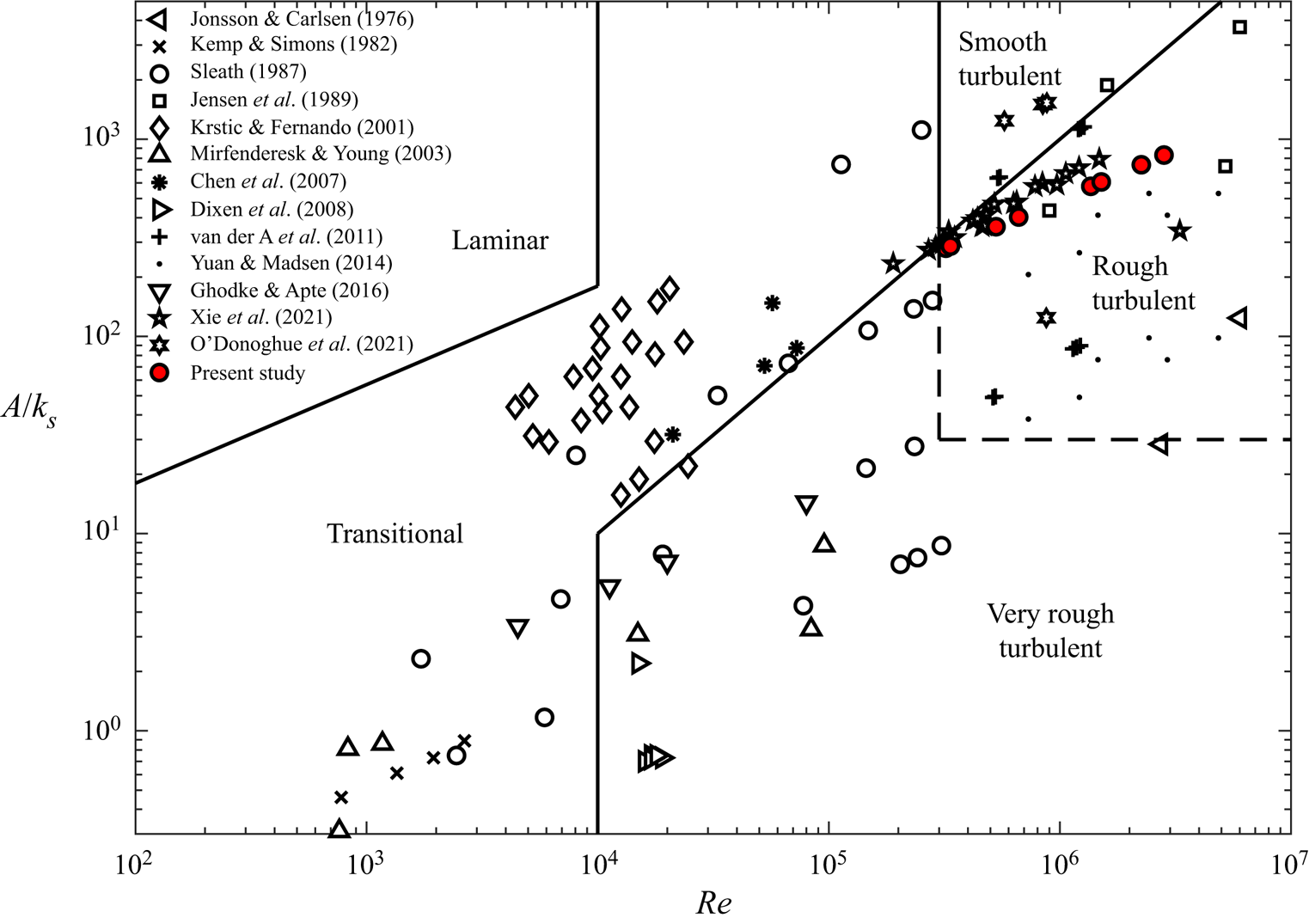
Figure 1. Delineation of flow regimes based on Jonsson (Reference Jonsson1966, Reference Jonsson1980) and Davies & Villaret (Reference Davies and Villaret1997), including the position of the test conditions from the present study and previous literature (Jonsson & Carlsen Reference Jonsson and Carlsen1976; Kemp & Simons Reference Kemp and Simons1982; Sleath Reference Sleath1987; Jensen, Sumer & Fredsøe Reference Jensen, Sumer and Fredsøe1989; Krstic & Fernando Reference Krstic and Fernando2001; Mirfenderesk & Young Reference Mirfenderesk and Young2003; Chen et al. Reference Chen, Chen, Tang, Stansby and Li2007; Dixen et al. Reference Dixen, Hatipoglu, Sumer and Fredsøe2008; van der A et al. Reference van der A, O'Donoghue, Davies and Ribberink2011; Yuan & Madsen Reference Yuan and Madsen2014; Ghodke & Apte Reference Ghodke and Apte2016; O'Donoghue et al. Reference O'Donoghue, Davies, Bhawanin and van der A2021; Xie et al. Reference Xie, Zhang, Li, Li, Yang, Zhang and Qu2021). Note that only the four regular (i.e. non-modulated) flows from O'Donoghue et al. (Reference O'Donoghue, Davies, Bhawanin and van der A2021) are included.
Existing knowledge of turbulent OBLs is derived from experimental studies performed in wave flume facilities (e.g. Sleath Reference Sleath1970; Cox, Kobayashi & Okayasu Reference Cox, Kobayashi and Okayasu1996; Dixen et al. Reference Dixen, Hatipoglu, Sumer and Fredsøe2008), oscillatory flow tunnels (e.g. Jonsson & Carlsen Reference Jonsson and Carlsen1976; Sleath Reference Sleath1987; Jensen et al. Reference Jensen, Sumer and Fredsøe1989) and facilities in which a wall is oscillated in a tank of fluid (e.g. Bagnold Reference Bagnold1946; Keiller & Sleath Reference Keiller and Sleath1976; Krstic & Fernando Reference Krstic and Fernando2001). Additionally, numerical simulation has been used to investigate turbulent OBLs, including  $k$–
$k$– $\varepsilon$,
  $k$–
$k$– $\omega$ (with k being the turbulent kinetic energy density,
  $\varepsilon$ the dissipation rate and
  $\omega$ the specific dissipation rate) and similar eddy-viscosity based models (e.g. Henderson, Allen & Newberger Reference Henderson, Allen and Newberger2004; Fuhrman, Fredsøe & Sumer Reference Fuhrman, Fredsøe and Sumer2009; Zhang et al. Reference Zhang, Zheng, Wang and Demirbilek2011), large eddy simulation (LES, e.g. Salon, Armenio & Crise Reference Salon, Armenio and Crise2007) and direct numerical simulation (DNS, e.g. Spalart & Baldwin Reference Spalart and Baldwin1987; Scandura, Faraci & Foti Reference Scandura, Faraci and Foti2016; Ghodke & Apte Reference Ghodke and Apte2018a). Most early OBL studies considered the case of sinusoidal oscillatory flow. However, oscillatory flows under sea waves in the coastal zone exhibit skewness and asymmetry to varying degrees due to shoaling and breaking processes (Malarkey & Davies Reference Malarkey and Davies2012), properties that are important for practical sediment transport applications (e.g. King Reference King1991; Dibajnia & Watanabe Reference Dibajnia and Watanabe1998; van der A, O'Donoghue & Ribberink Reference van der A, O'Donoghue and Ribberink2010; Silva et al. Reference Silva, Abreu, van der A, Sancho, Ruessink, van der Werf and Ribberink2011). More recently, van der A et al. (Reference van der A, O'Donoghue, Davies and Ribberink2011), Yuan & Madsen (Reference Yuan and Madsen2014) and O'Donoghue et al. (Reference O'Donoghue, Davies, Bhawanin and van der A2021) studied the hydrodynamics of rough-wall OBL flows with significant skewness or asymmetry. To the authors’ knowledge, no previous studies have systematically investigated flows that simultaneously possess both skewness and asymmetry to a significant degree.
Several OBL studies (e.g. Spalart & Baldwin Reference Spalart and Baldwin1987; Scandura Reference Scandura2007; Scandura et al. Reference Scandura, Faraci and Foti2016; van der A, Scandura & O'Donoghue Reference van der A, Scandura and O'Donoghue2018; Fytanidis, García & Fischer Reference Fytanidis, García and Fischer2021; Mier, Fytanidis & García Reference Mier, Fytanidis and García2021) considered the simplified case of flow over a smooth wall. For practical OBLs that occur in the coastal zone, the seabed is rough, composed of sediment particles. Sleath (Reference Sleath1987) conducted oscillatory flow tunnel experiments over beds of sand, gravel and pebbles and showed that, for small  $A/k_{s}$, contrary to the case of a smooth wall, the phase-averaged Reynolds shear stress
  $-\overline {u'v'}$ (
 $u$ and
  $v$ are streamwise and wall-normal velocity, respectively; overbar denotes a phase average;
  $'$ denotes the fluctuation relative to the phase average) was much smaller than the total shear stress obtained by integration of the momentum equation, attributing the discrepancy to periodic ‘jets’ caused by vortex formation and ejection at flow reversal. Velocity in direction
  $i$,
$i$,  $u_{i}$, can be decomposed as
  $u_{i}=\langle \bar {u}_{i}\rangle +\tilde {u}_{i}+u_{i}'$, where angle brackets denote an intrinsic spatial average (hereafter referred to as just ‘spatial average’ for brevity) and tilde is the fluctuation of the phase average with respect to the spatial average. Applying this decomposition to the Navier–Stokes equations and then taking the phase- and spatial-average results in the double-averaged Navier–Stokes (DANS) equations (e.g. Nikora et al. (Reference Nikora, McEwan, McLean, Coleman, Pokrajac and Walters2007), note that the DANS equations obtained from the phase and spatial average are analogous to those obtained from the time and spatial average). The DANS equations contain expressions for the dispersive and Reynolds stresses
  $-\langle \tilde {u}_{i}\tilde {u}_{j}\rangle$ and
  $-\langle \overline {u_{i}'u_{j}'}\rangle$, which arise due to flow inhomogeneity and turbulent fluctuations, respectively. Using DANS equations, Giménez-Curto & Corniero Lera (Reference Giménez-Curto and Corniero Lera1996) confirmed that Reference SleathSleath's (Reference Sleath1987) findings could be explained by the presence of dispersive stresses resulting from flow separation from roughness elements. Ghodke & Apte (Reference Ghodke and Apte2018a) utilised the DANS equations to investigate the effect of roughness on momentum transfer mechanisms in oscillatory flow in the transitional and very rough turbulent regimes. Using DNS, they showed that dispersive stresses were significant mainly below roughness crests and up to twice the roughness diameter above roughness crests for larger and smaller hexagonally packed spherical roughness elements, respectively. Using the budget equations for the turbulence kinetic energy (TKE) and wake kinetic energy (WKE), they also investigated the mechanisms responsible for generation, redistribution and dissipation of TKE and WKE. Further study is necessary to obtain a deeper understanding of these mechanisms in rough-wall OBL flow.
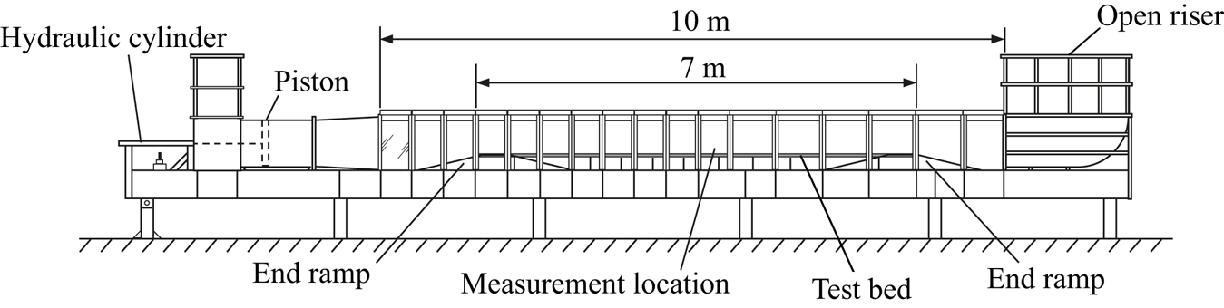
Figure 2. The Aberdeen Oscillatory Flow Tunnel.
Some steady flow sediment transport models incorporate a stochastic description of turbulence (e.g. Shi & Yu Reference Shi and Yu2015; Cheng et al. Reference Cheng, Chauchat, Hsu and Calantoni2018). These models assume a Gaussian probability density function (PDF) of turbulent velocity fluctuations which is not always true in reality. Much of the current understanding of turbulence statistics in wall-bounded flows comes from experimental and numerical studies of steady, turbulent flow in open channels, pipes and in the vicinity of a wall (e.g. Kreplin & Eckelmann Reference Kreplin and Eckelmann1979; Kim, Moin & Moser Reference Kim, Moin and Moser1987; Alfredsson et al. Reference Alfredsson, Johansson, Haritonidis and Eckelmann1988; Barlow & Johnston Reference Barlow and Johnston1988; Durst, Jovanovic & Sender Reference Durst, Jovanovic and Sender1995). These studies investigated the relative intensity  $R_{u'}=\langle \overline {u^{'2}}\rangle ^{1/2}/\langle \bar {u}\rangle$, skewness
  $S_{u'}=\langle \overline {u^{'3}}\rangle /\langle \overline {u^{'2}}\rangle ^{3/2}$ and kurtosis (also known as flatness)
  $K_{u'}=\langle \overline {u^{'4}}\rangle /\langle \overline {u^{'2}}\rangle ^{2}$ of velocity fluctuations (definitions of streamwise statistics are shown; analogous expressions exist for the wall-normal and spanwise statistics). To date, relatively little work has been performed investigating the turbulence statistics for oscillatory flows, particularly for rough walls. Hino et al. (Reference Hino, Kashiwayanagi, Nakayama and Hara1983) conducted smooth-wall oscillatory wind tunnel experiments and found that while the fundamental processes by which turbulence is generated are almost the same as in steady flow, the turbulence statistics differed ‘remarkably’ from the steady flow case. The PDFs of
  $u'$, were skewed during most of the decelerating part of the flow cycle, and PDFs of
  $u'$ and
  $v'$ had elongated lobes during the ejection and wallward interaction phases of the cycle. More recently, Scandura et al. (Reference Scandura, Faraci and Foti2016) conducted DNS of asymmetric oscillatory flow over a smooth wall for
  $R_{\delta }=1100$ and
  $1414$, where the Stokes length Reynolds number
  $R_{\delta }=U\delta /\nu$ and
  $\delta =\sqrt {2\nu /\omega }$ is the Stokes length. They found that low-speed streaks of fluid were generated along the streamwise direction which broke up towards the end of the accelerating phase of each half-cycle. The PDFs of the frequency distribution of streamwise and spanwise shear stress were well approximated by a log-normal and Pearson type VII distribution, respectively. During break-up of streamwise streaks, the appearance of a sharp peak resulted in a generalised normal distribution being more applicable to describe the PDF of spanwise shear stress. van der A et al. (Reference van der A, Scandura and O'Donoghue2018) conducted oscillatory flow tunnel (OFT) experiments for turbulent oscillatory flow over a smooth wall, with three of their flow conditions complemented by DNS. They showed that the skewness and kurtosis of velocity fluctuations in the vicinity of the wall reached very large values during part of the acceleration phase of each half-cycle, which coincided with the existence of streamwise-elongated low-speed streaks similar to those reported by Scandura et al. (Reference Scandura, Faraci and Foti2016), leading to significant flow intermittency. At the phase when the streaks broke down, the skewness and kurtosis returned to much smaller values. Near the wall, the PDFs of
  $u'$,
$u'$,  $v'$ and
  $w'$, where
  $w$ is spanwise velocity, were approximately described by log-normal, Pearson type IV and Pearson type VII distributions, respectively. Current knowledge of the turbulence statistics in rough-wall OBL flow is very limited. Ghodke & Apte (Reference Ghodke and Apte2016) performed DNS over an idealised rough wall consisting of hexagonally arranged spherical elements and obtained PDFs of turbulent velocity and pressure fluctuations at the phase of peak free-stream velocity which were well approximated by a fourth-order Gram–Charlier distribution, which was shown to also describe the PDFs of drag and lift force on the spherical particles by Ghodke & Apte (Reference Ghodke and Apte2018b). The statistics of OBL flow over a more realistic irregular rough wall have yet to be investigated in detail.
This paper seeks to further current understanding of turbulence statistics and momentum transfer mechanisms in OBL flow over a rough wall representative of a gravel seabed. This is achieved using a combination of OFT experiments and DNS.
The present set of DNS distinguishes itself from previous DNS studies of oscillatory flow over a rough wall (see table 1) in that (i) the roughness is irregular and is comprised of elements based on the shapes of real gravel particles, (ii)  $R_{\delta }$ extends to values significantly higher than previous studies and (iii) a range of oscillatory flow shapes are studied, in contrast with the previous studies for which all the flows were sinusoidal. Experiments are performed using the same irregular rough wall to validate numerical simulations and to allow flows with Reynolds numbers larger than could be practically simulated using DNS to be investigated. The structure of the paper is as follows. Section 2 illustrates the experimental set-up, instrumentation and data processing. Section 3 describes the numerical procedure, validation and data handling. Section 4 reports on key features of the ensemble-averaged flow and compares with previous literature. The turbulence structure is visualised using isosurfaces of
  $\lambda _{2}$ (Jeong & Hussain Reference Jeong and Hussain1995) in § 5. Features of the Reynolds and dispersive stresses are explored in § 6. The statistics of turbulent velocity fluctuations are investigated in § 7. Finally, the paper is concluded in § 8 with a summary of key findings.
Table 1. Comparison of present study with previous DNS studies of oscillatory flow over rough walls. Note that the roughness used by Mazzuoli et al. (Reference Mazzuoli, Blondeaux, Simeonov and Calantoni2018) was irregular, consisting of spheres fitted to a scanned sediment bed profile, although each individual roughness element was an identical smooth sphere.

2. Experimental methodology
2.1. Test facility
Experiments were performed in the Aberdeen Oscillatory Flow Tunnel (AOFT, figure 2, e.g. van der A et al. Reference van der A, O'Donoghue, Davies and Ribberink2011), a U-tube facility 16 m in length, with a 10 m long, 0.75 m high and 0.3 m wide test section containing a 7 m long polyvinyl chloride (PVC) test bed raised 0.25 m by a stainless steel frame. End reservoirs are both open to atmosphere. Flow is generated by a 0.75 m diameter piston driven by a 30 kW electro-hydraulic system with 1 m stroke length. A proportional control valve allows any time-varying flow within the mechanical capabilities of the drive system to be generated in the facility.
A rough wall composed of repetitions of the element shown in figure 3 was attached to the PVC test bed in the AOFT. This element has periodic boundaries and is based on a high-resolution scan of real gravel particles with median grain diameter  $d_{50}=2.81$ mm, made using a Micro-Epsilon ConfocalDT IFS2405-10 confocal sensor with vertical resolution of 386 nm mounted on a high-precision 3-axis traverse system. The rough wall consisted of 22 cast epoxy resin tiles, each comprised of 28 periodic elements arranged in a
  $4\times 7$ (
 ${\rm streamwise}\times {\rm spanwise}$) pattern (see figure 5). The tiles were fixed to the PVC test bed with double-sided tape. More details of the design and manufacture of the experimental roughness are presented in Dunbar (Reference Dunbar2022).
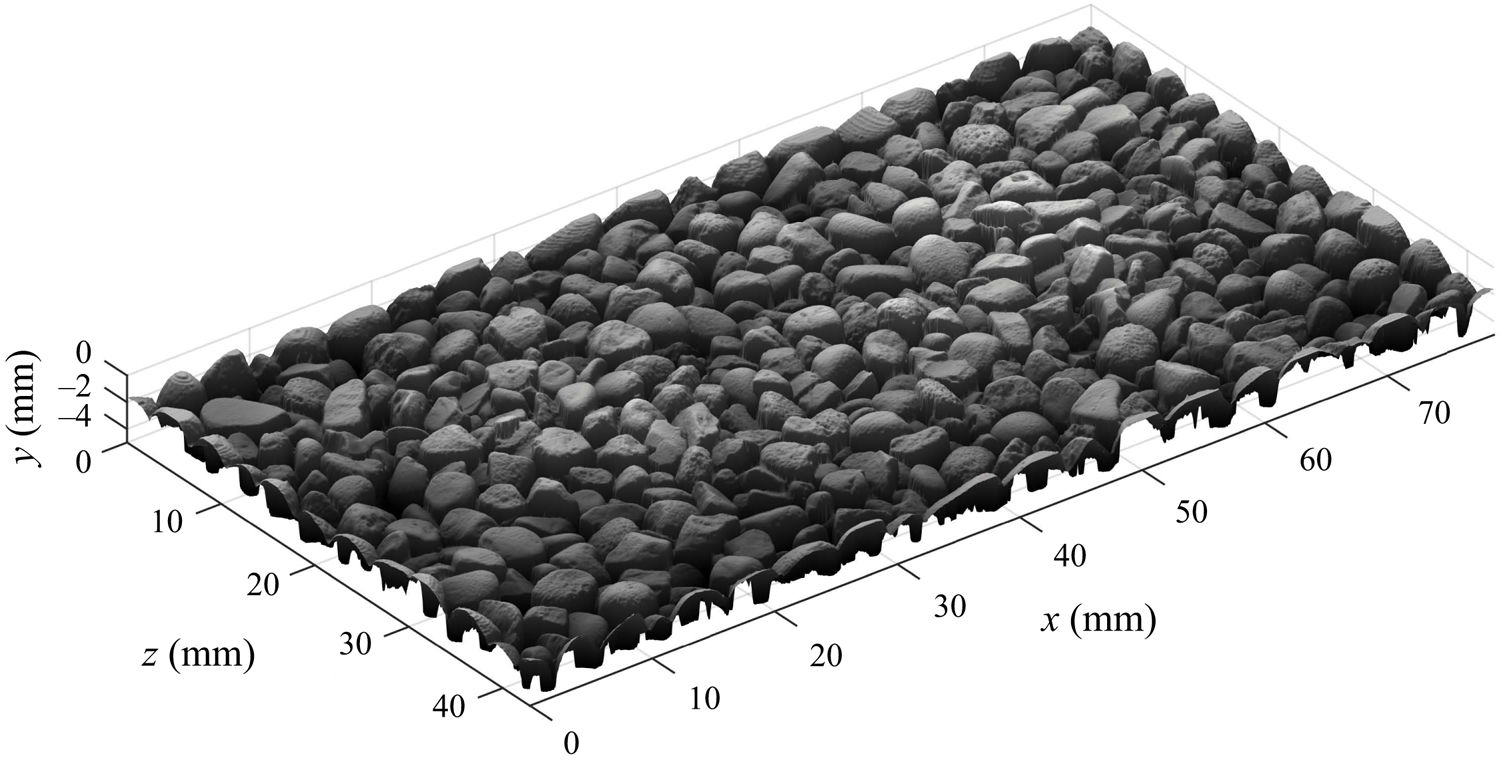
Figure 3. Illustration of periodic gravel roughness element;  $x$,
$x$,  $y$ and
  $z$ are streamwise, wall-normal and spanwise coordinates, respectively.
2.2. Instrumentation
Velocity measurements were made using a 2-component laser-Doppler anemometry (LDA) system comprising (i) a 300 mW Dantec Dynamics Modu-laser Stellar-Pro-L Select air-cooled argon-ion laser; (ii) a Dantec Dynamics FiberFlow transmitter with an integrated Bragg cell; (iii) a 112 mm diameter probe containing the laser emission and receiving optics and fitted with a 310 mm focal length (in air) lens, resulting in a measurement volume with maximum diameter of 47 $\,\mathrm {\mu }$m and spanwise length of 530
 $\,\mathrm {\mu }$m; (iv) an isel 3-axis stepper-motor driven traverse system to which the probe was fitted, allowing the probe to be positioned in increments of 12.5
 $\,\mathrm {\mu }$m, accurate to within 10
 $\,\mathrm {\mu }$m (van der A et al. Reference van der A, Scandura and O'Donoghue2018); (v) a Dantec Dynamics F60 burst spectrum analyser (BSA); and (vi) a computer running Dantec Dynamics BSA flow software 5.20.03 used to control the BSA settings, traverse system and the data acquisition.
For all measurements, the LDA system was set up in a backscatter configuration. The two velocity components were measured coincidently at approximately 45 $^{\circ }$ relative to the streamwise direction to maximise the data acquisition rate. In order to measure at positions very close to the wall, the probe was tilted forwards by
  $3.9$–
 $4.5^{\circ }$ to ensure that the lower beam in each LDA component pair was not blocked by asperities. As a result, the ‘wall-normal’ component of velocity is not truly wall normal but tilted
  $3.9$–
 $4.5^{\circ }$ relative to the wall-normal direction. Practically speaking, this small forward tilt can be neglected because
  $\sin (3.9^{\circ })=0.068\approx 0$,
  $\cos (3.9^{\circ })=0.998\approx 1$,
  $\sin (4.5^{\circ })=0.079\approx 0$ and
  $\cos (4.5^{\circ })=0.997\approx 1$. The flow was seeded with hollow glass microspheres (Potters Sphericel 110P8) with a median diameter of 9–11
 $\,\mathrm {\mu }$m and density of
  $1100\pm 50$ kg m
 $^{-3}$.
2.3. Flow conditions
The piston in the AOFT was programmed to generate oscillatory flow in the test section with oscillatory velocity in the free stream following the description of Abreu et al. (Reference Abreu, Silva, Sancho and Temperville2010). Velocities were measured for 8 conditions comprising 2 values of Reynolds number  $R_{\delta,\sigma }=\sqrt {2}U_{\sigma }\delta /\nu$, where
  $U_{\sigma }$ is the standard deviation of the free-stream velocity, and 4 flow shapes, as detailed in table 2. Note that the free-stream energy integrated over one flow cycle is the same for any two flows with the same value of
  $R_{\delta,\sigma }$. Experiments are identified by a 6 character name, as follows:
 \begin{equation} \underbrace{\text{SS}}_{\text{flow shape}}\underbrace{0800}_{\text{target } R_{\delta,\sigma}}. \end{equation}
Flow shape identifiers denote sinusoidal (SS), skewed (SK), combined skewed and asymmetric (CB) and asymmetric (AS).
Table 2. Summary of test conditions. Subscript  $_{\infty }$ denotes a quantity in the free stream. The
  $A/k_{s}$ values reported were computed using
  $k_{s}$ obtained from the procedure detailed in § 4.1. Note that actual values of
  $R_{\delta,\sigma }$ do not exactly match the target values, and flow shapes SS and SK (SS and AS) possess a small, non-zero
  ${\textit {As}}_{\infty }$ (
 ${\textit {Sk}}_{\infty }$) value. This is due to the inability of the experimental facility to perfectly reproduce the target flow conditions.
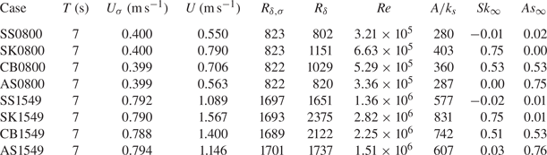
Table 2 shows the flow conditions measured in the test section of the AOFT. Free-stream skewness  ${\textit {Sk}}_{\infty }$ and asymmetry
  ${\textit {As}}_{\infty }$ were computed using
 \begin{equation} {\textit{Sk}}_{\infty}=\frac{\overline{\overline{(u-\bar{\bar{u}})^{3}}}}{\overline{\overline{(u-\bar{\bar{u}})^{2}}}^{{3}/{2}}}, \end{equation}
and
 \begin{equation} {\textit{As}}_{\infty}={-}\frac{\overline{\overline{[\mathcal{H}(u-\bar{\bar{u}})]^{3}}}}{\overline{\overline{(u-\bar{\bar{u}})^{2}}}^{{3}/{2}}}, \end{equation}
respectively (e.g. Malarkey & Davies Reference Malarkey and Davies2012; van der A et al. Reference van der A, Scandura and O'Donoghue2018), where the double overbar denotes the time average and  $\mathcal {H}$ is the Hilbert transform. The free-stream elevation was taken as the highest measurement position for each set of vertical profile measurements (
 $y=75$ and 100 mm for cases with target
  $R_{\delta,\sigma }=800$ and
  $R_{\delta,\sigma }=1549$, respectively; see § 2.4). The measured free-stream velocity for each flow condition is shown in figure 4. Reynolds numbers were computed based on
  $\nu =1.05\times 10^{-6}$ and
  $\nu =0.97\times 10^{-6}$ m
 $^{2}$ s
 $^{-1}$ for flows with target
  $R_{\delta,\sigma }=800$ and
  $R_{\delta,\sigma }=1549$, respectively, corresponding to the average water temperature measured using a digital thermometer during the respective experiments.
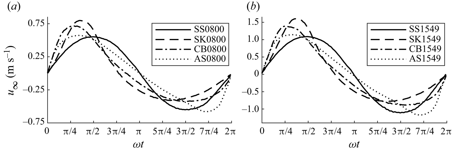
Figure 4. Measured intra-period free-stream velocity for flow cases with target  $R_{\delta,\sigma }=800$ (a) and
  $R_{\delta,\sigma }=1549$ (b). Here,
  $t$ is the intra-period time.
2.4. Measurement locations
All measurements were made above a single periodic element. Figure 5 shows the measurement tile and the individual element over which measurements were made. Note that measurements were not made at the tunnel centreline because of increased attenuation of LDA laser light at locations farther from the LDA probe. Measurements were made above the indicated periodic element because it was far from the influence of the sidewalls, while being close enough to the LDA probe to allow for good measurement quality. The coordinate system for the measurement positions was as shown in figure 3, where  $y=0$ corresponds to the vertical position of the highest roughness crest. In order to align the LDA measurement volume with the coordinate system, the measurement volume was aligned with a reference position, taken as the highest roughness crest, which could be distinguished by eye and the coordinates of which were known a priori. This was achieved by traversing the LDA probe in 50
 $\,\mathrm {\mu }$m increments after positioning the measurement volume close to the reference position by eye. The precise location of the reference position was taken as the highest position where the local reflection of laser light detected by the photomultiplier was a local maximum. In the case of multiple such positions, the local maximum with the largest detected reflection was selected.
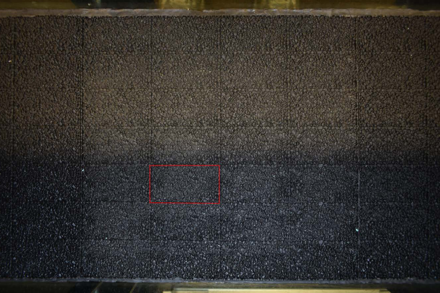
Figure 5. Plan view of the epoxy resin roughness tile at the measurement location inside the AOFT test section. The periodic element over which all measurements were made is highlighted by the red lines. The bottom of the image corresponds to the near side of the AOFT adjacent to which the LDA probe was positioned.
Two sets of measurements were made: (i) vertical profiles of velocity were measured above the centre of the periodic element ( $x=39.4$,
  $z=21.4$ mm) at 25 logarithmically spaced vertical positions between
  $y=0.1$ and
  $y=75$ (
 $100$) mm above the highest roughness crest for cases with target
  $R_{\delta,\sigma }=800$ (
 $1549$). Measurements were taken for 150 flow cycles at the lowest 14 elevations and 100 cycles at the remaining 11 elevations. The aim of these measurements was to obtain vertical profiles of phase-averaged velocity and converged second-order turbulence statistics. (ii) Velocity measurements were also taken for 500 flow cycles at 9 positions distributed evenly in the horizontal plane at
  $y=0.5$ and
  $y=3$ mm for all flow cases. The aim of these measurements was to obtain converged third- and fourth-order turbulence statistics in the vicinity of the roughness.
2.5. Data processing
Velocity data obtained from the LDA system were validated by the BSA during data acquisition. Two parameters set in the BSA software control whether a Doppler burst is rejected by the BSA: burst spectrum signal-to-noise level and validation ratio. The validation ratio is defined as the ratio between the two highest spectral peaks of a given Doppler burst; if the ratio is below a threshold value, the burst is rejected. Increasing the signal-to-noise and validation ratios results in higher data quality at the cost of lower data rate. The burst spectrum signal-to-noise level was set to 2 dB for all measurements and the validation ratio was set to 8 for the vertical profile measurements and 10 for the near-roughness measurements. These values were determined using trial and error as a good compromise between data quality and data rate. With these settings, acquired data were of high quality and very little additional outlier removal was necessary. Typical data rates ranged from  ${\approx }75$ Hz very near the roughness, up to
  ${\approx }225$ Hz in the free stream. Any outliers not rejected by the BSA were identified as data that deviate more than 6 standard deviations from the mean within a particular phase bin and were removed during the phase-averaging process. Such outliers made up less than 0.003 % of the acquired data.
Phase-averaged streamwise velocity, accounting for particle residence time weighting (Buchhave, George & Lumley Reference Buchhave, George and Lumley1979), was computed using
 \begin{align} \bar{u}(x,y,z,\omega t)&=\frac{\displaystyle\sum_{n=1}^{N_{{T}}} \sum_{m=1}^{M_{{T}}}u_{m}(x,y,z,\phi_{{B}}+[n-1]2{\rm \pi})t_{{r},m} (x,y,z,\phi_{{B}}+[n-1]2{\rm \pi})}{\displaystyle\sum_{n=1}^{N_{{T}}} \sum_{m=1}^{M_{{T}}}t_{{r},m}(x,y,z,\phi_{{B}}+[n-1]2{\rm \pi})} \nonumber\\ &\quad\text{for } 0\leq \omega t<2{\rm \pi}, \end{align}
where  $N_{{T}}$ is the total number of flow cycles at position
  $(x,y,z)$,
  $M_{{T}}$ is the total number of samples in the phase bin,
  $\phi _{{B}}$ is the phase bin
  $\omega t\leq \phi _{{B}}<\omega t+\delta \tau$,
  $\delta \tau =2{\rm \pi} /(f_{{s}}T)$,
  $f_{{s}}$ is a nominal sampling frequency set to 32 Hz in the case of the present experimental work and
  $t_{{r}}$ is the residence time of the seeding particle in the measurement volume, recorded by the LDA system. An analogous equation was used to obtain
  $\bar {v}(x,y,z,\omega t)$. The double-averaged streamwise velocity was computed using
 \begin{equation} \langle\bar{u}\rangle(y,\omega t)=\frac{1}{N_{x}N_{z}}\sum_{l=1}^{N_{x}} \sum_{k=1}^{N_{z}}\bar{u}(x_{l},y,z_{k},\omega t), \end{equation}
where  $N_{x}$ and
  $N_{z}$ are the number of measurement positions along
  $x$ and
  $z$, respectively. An analogous equation was used to obtain
  $\langle \bar {v}\rangle (y,\omega t)$. In the case of the vertical profile measurements,
  $N_{x}=N_{z}=1$ so a spatial average was not computed. In the case of the horizontal plane measurements,
  $N_{x}=N_{z}=3$.
The root-mean-square of streamwise fluctuations,  $u_{{rms}}^{'}$, was computed using
 \begin{align} & u_{{rms}}^{'}(y,\omega t) \nonumber\\ &\quad =\frac{1}{N_{x}N_{z}}\sum_{l=1}^{N_{x}}\sum_{k=1}^{N_{z}} \sqrt{\frac{\displaystyle\sum_{n=1}^{N_{{T}}}\sum_{m=1}^{M_{{T}}}u_{m}^{'2} (x,y,z,\phi_{{B}}+[n-1]2{\rm \pi})t_{{r},m}(x,y,z,\phi_{{B}}+[n-1]2{\rm \pi})}{\displaystyle\sum_{n=1}^{N_{{T}}} \sum_{m=1}^{M_{{T}}}t_{{r},m}(x,y,z,\phi_{{B}}+[n-1]2{\rm \pi})}} \nonumber\\ &\qquad\text{for } 0\leq \omega t<2{\rm \pi}, \end{align}
where local streamwise turbulent fluctuations are given by
 \begin{equation} u_{m}^{'}(x,y,z,\phi_{{B}}+[n-1]2{\rm \pi})=u_{m}(x,y,z,\phi_{{B}}+[n-1]2{\rm \pi})-\bar{u}(x,y,z,\omega t). \end{equation}
Analogous equations were used to compute third- and fourth-order statistics and Reynolds shear stress. The statistics of the wall-normal turbulence were also computed using analogous equations, replacing  $u$ with
  $v$. Further details of the experimental methodology and data processing are given in Dunbar (Reference Dunbar2022).
3. Numerical methodology
3.1. Numerical conditions
The numerical domain is shown in figure 6 (note that, in the coordinate system used for DNS,  $y=0$ corresponds to the bottom of the domain; DNS results are vertically shifted in post-processing to align with the coordinate system used for experimental measurements, where
  $y=0$ corresponds to the vertical position of the highest roughness crest). The domain consists of a Cartesian box with dimensions
  $L_{x}/\delta =52.739$,
  $L_{y}/\delta =50.000$ and
  $L_{z}/\delta =28.711$. The periodic gravel roughness shown in figure 3 is positioned at the bottom of the domain with a vertical offset of
  $0.001\delta$ to ensure that no points in the height field intersect the bottom of the domain. Periodic boundary conditions are applied in the streamwise and spanwise directions, with a zero-shear boundary condition on the upper boundary. The no-slip condition is imposed on the surface of the roughness using an immersed boundary method similar to Orlandi & Leonardi (Reference Orlandi and Leonardi2006).
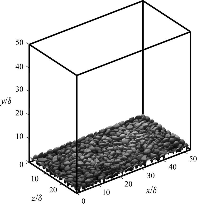
Figure 6. Sketch of the numerical domain.
Simulations were conducted for the first 4 flow conditions shown in table 2. This was achieved using a driving pressure gradient consistent with the free-stream velocity measured in the AOFT test section following van der A et al. (Reference van der A, Scandura and O'Donoghue2018).
Table 3 shows the grid characteristics used for each simulation case. The numerical domain is discretised onto a regular Cartesian grid along directions  $x$ and
  $z$. A three-layer grid spacing scheme is applied along direction
  $y$. Between elevations corresponding to the mean and maximum value of the roughness height field, grid spacing is constant and equal to
  ${\rm \Delta} y_{{min}}$. Outside this layer, spacing increases with distance according to a hyperbolic tangent function. The grid spacings shown in table 3 are comparable to previous DNS studies of turbulent flow over a rough wall (e.g. Ikeda & Durbin Reference Ikeda and Durbin2007; Cardillo et al. Reference Cardillo, Chen, Araya, Newman, Jansen and Castillo2013; Yuan & Piomelli Reference Yuan and Piomelli2015; Ghodke & Apte Reference Ghodke and Apte2018a) in terms of Kolmogorov length scales and wall units.
Table 3. Numerical grid characteristics used for each simulation case. Here,  $n_{i}$ is number of cells in direction
  $i$,
$i$,  ${\rm \Delta} i$ is grid spacing in direction
  $i$,
$i$,  $\eta$ is the Kolmogorov length scale and superscript
  $^{+}$ denotes a quantity in wall units. Note that the values of
  $n_{y}$ differ between flow cases because the spatial resolution requirement increases with
  $R_{\delta }$.

3.2. Numerical procedure
The dimensionless continuity and Navier–Stokes equations are solved using a fractional-step method based on Kim & Moin (Reference Kim and Moin1985) and Mohan Rai & Moin (Reference Mohan Rai and Moin1991). Convective and viscous terms are discretised using an explicit 3-step Runge–Kutta scheme and the implicit second-order Crank–Nicolson scheme, respectively. The numerical code is written in FORTRAN and parallelised using OpenMP, and has been used for several previous oscillatory flow studies (e.g. Scandura Reference Scandura2007; Scandura et al. Reference Scandura, Faraci and Foti2016; van der A et al. Reference van der A, Scandura and O'Donoghue2018).
Simulation case SK0800 was conducted using an HP Z4 workstation with a 10-core 3.3 GHz Intel i9-9820X CPU and 64 GB of RAM at the University of Aberdeen, and cases SS0800, CB0800 and AS0800 were conducted using 2 Supermicro servers each with four 8-core 2.3 GHz Intel Xeon E5-4610 v2 CPUs and 251 GB of RAM at the University of Catania. Approximately  $3\times 10^5$ CPU hours were required in total for all simulation cases. During simulation, files containing all three velocity components and pressure at each grid point were saved at 32 uniformly distributed times within each flow period for post-processing.
3.3. Verification and validation
Sufficiency of the size of the numerical domain was verified by checking that the spatial autocorrelation function of each fluctuating velocity component along  $x$ and
  $z$ decayed to small values within half of the size of the computational domain. Additionally, the height of the numerical domain was found to be at least
  $4.4\delta _{{bl}}$ in all simulation cases, where
  $\delta _{{bl}}$ is the boundary layer thickness defined as the elevation of maximum velocity overshoot at the phase corresponding to maximum free-stream velocity (Jensen et al. Reference Jensen, Sumer and Fredsøe1989), confirming that the height of the domain is sufficient to resolve the boundary layer.
Adequacy of the numerical grid resolution was ensured by computing the continuous energy spectra of each fluctuating velocity component along  $x$ and
  $z$. Similar to van der A et al. (Reference van der A, Scandura and O'Donoghue2018), energy at high wavenumbers was found to be at least 4 orders of magnitude smaller than at low wavenumbers in all cases, confirming the adequacy of the numerical grid resolution.
For each flow case, 15–21 flow cycles were simulated. This was found to be sufficient to obtain converged ensemble-averaged third- and fourth-order turbulence statistics.
As noted by van der A et al. (Reference van der A, Scandura and O'Donoghue2018), the steady streaming (i.e. time-averaged streamwise velocity) generated by non-sinusoidal flow in an OFT facility differs from that in non-sinusoidal oscillatory flow driven by a periodic pressure gradient over a periodic domain, as is the case with the present DNS, due to the boundary conditions at the streamwise ends of the OFT. To match the DNS exactly to the measurements would require simulation of flow inside the entire AOFT, which would entail infeasible computational expense. Instead, streamwise velocities can be compared after first subtracting the steady streaming in each case, following van der A et al. (Reference van der A, Scandura and O'Donoghue2018). For example, figure 7 compares vertical profiles of ensemble-averaged streamwise velocity at 4 phases between DNS and measurements for case SK0800, before and after steady streaming is subtracted. The figure shows that there are discrepancies in ensemble-averaged streamwise velocity between DNS and measurements that vanish after the streaming is removed, justifying this approach.
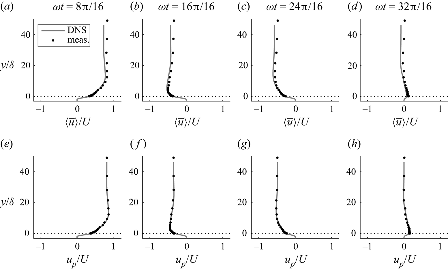
Figure 7. Comparison of DNS and measured vertical profiles of ensemble-averaged (a–d) and oscillatory (e–h) streamwise velocity at 4 phases for case SK0800 ( $u_{{p}}=\langle \bar {u}\rangle -\bar {\bar {u}}$; note that measured profiles are not averaged in space).
Example results demonstrating validation of several key turbulent flow quantities, including higher-order statistics, are shown in figures 8 and 9 for case SK0800. Figures showing similar agreement between DNS and measurements are obtained for the other three flow cases, but are omitted for brevity. Figure 8 compares vertical profiles of second-order turbulent quantities between DNS and measurements at 4 phases for case SK0800. Overall, the agreement is good, although discrepancies are visible for  $u'_{{rms}}$ and
  $v'_{{rms}}$ far from the roughness. It is possible that this is due to additional sources of turbulence in the experiment, such as the driving mechanism of the AOFT, that are not present in the DNS. This additional turbulence does not appear to be associated with vertical shear, since it does not affect the profiles of Reynolds shear stress
  $-\langle \overline {u'v'}\rangle$. Another possibility is that this results from noise in the LDA measurements, since noise would become more significant relative to the ‘true’
  $u'$ and
  $v'$ values at large
  $y/\delta$. This effect would appear in
  $u'_{{rms}}$ and
  $v'_{{rms}}$ but not in
  $-\langle \overline {u'v'}\rangle$ because the noise is uncorrelated. Very near the roughness, some discrepancies are also visible, particularly at phase
  $\omega t=8{\rm \pi} /16$. These discrepancies can be attributed to the lack of spatial averaging in the measured profiles, which becomes significant very near the roughness where the flow is not homogeneous, particularly at phases corresponding to large ensemble-averaged velocity magnitude, as is the case at
  $\omega t=8{\rm \pi} /16$.
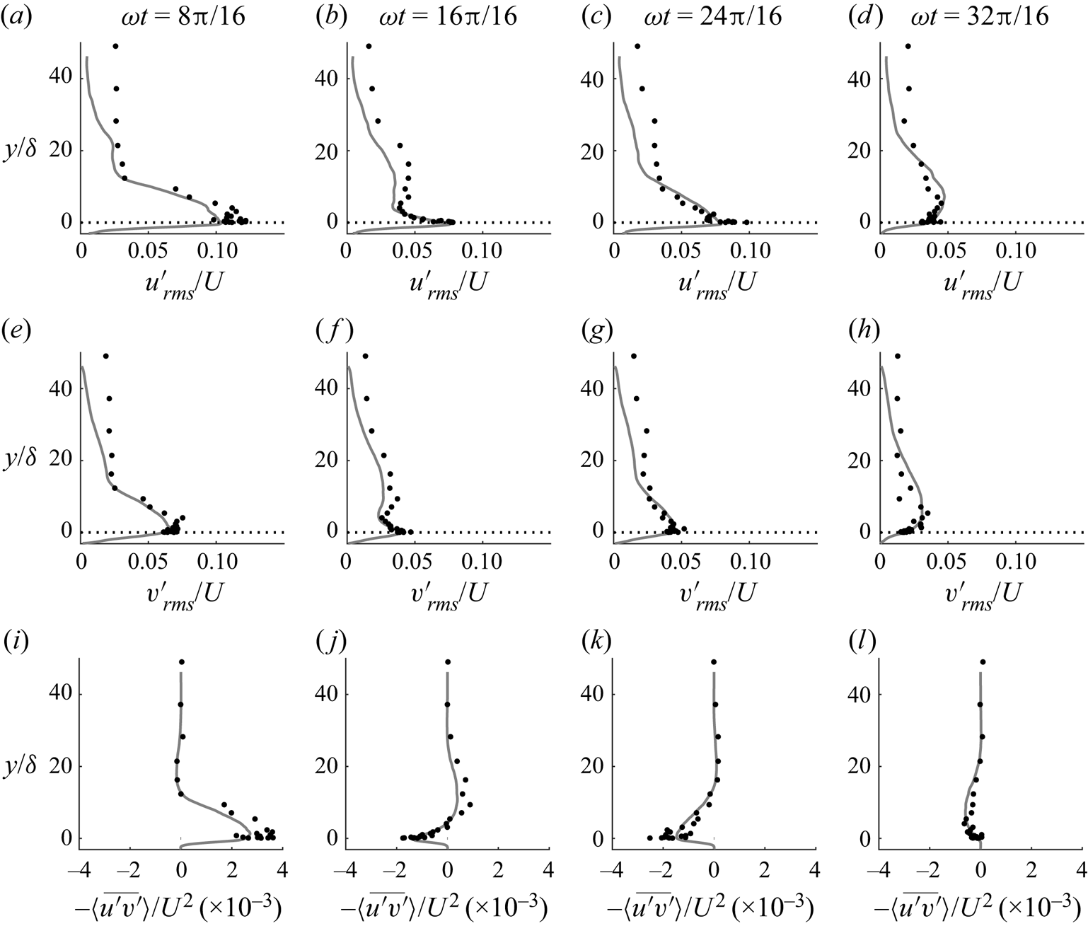
Figure 8. Comparison of DNS and measured vertical profiles of the root-mean-square of streamwise (a–d) and wall-normal (e–h) fluctuations and Reynolds shear stress (i–l) at 4 phases for case SK0800. Profiles are averaged in phase (both measurements and DNS) and space (DNS only). Line styles are as in figure 7.

Figure 9. Comparison of DNS and measured intra-period skewness (a,b) and kurtosis (c,d) of streamwise (a,c) and wall-normal (b,d) velocity fluctuations at  $y=0.5$ mm for case SK0800. Both DNS and measurements are averaged in phase and space. Line styles are as in figure 7.
Figure 9 compares intra-period higher-order turbulence statistics between DNS and measurements at a location very near to the roughness. In the DNS case, the statistics are computed only at the 32 phases at which results files are saved, which results in the lack of smoothness observed in the solid lines. Remarkably good agreement is seen between DNS and measurements, considering the sensitivity of third- and fourth-order statistical moments to any outliers in the data.
Further details regarding the numerical methodology, verification and validation can be found in Dunbar (Reference Dunbar2022).
4. Ensemble-averaged velocities
4.1. Determination of equivalent sandgrain roughness length,  $k_{s}$

Many studies have shown that the classical ‘law of the wall’ can be applied to oscillatory flows (e.g. Jonsson & Carlsen Reference Jonsson and Carlsen1976; Sleath Reference Sleath1987; Jensen et al. Reference Jensen, Sumer and Fredsøe1989; Cox et al. Reference Cox, Kobayashi and Okayasu1996; Dixen et al. Reference Dixen, Hatipoglu, Sumer and Fredsøe2008; van der A et al. Reference van der A, O'Donoghue, Davies and Ribberink2011; Yuan & Madsen Reference Yuan and Madsen2014; Ghodke & Apte Reference Ghodke and Apte2016; Scandura et al. Reference Scandura, Faraci and Foti2016). For flow over a rough wall, (4.1)–(4.3) (Ligrani & Moffat Reference Ligrani and Moffat1986) describe the velocity in the logarithmic layer
 \begin{gather} u^{+}=\frac{1}{\kappa}\ln[(y+d')^{+}]+C+{\rm \Delta} u^{+} \end{gather}
 \begin{gather}{\rm \Delta} u^{+}=\left[8.5-C-\frac{1}{\kappa}\ln({\textit{Re}}_{k})\right]\sin\left(\frac{{\rm \pi} g_{{lm}}}{2}\right) \end{gather}
 \begin{gather}g_{{lm}}= \begin{cases} 0 & \text{for}\ {\textit{Re}}_{k}<{\textit{Re}}_{k,{s}} \\ \dfrac{\ln({\textit{Re}}_{k}/{\textit{Re}}_{k,{s}})}{\ln({\textit{Re}}_{k,{r}}/{\textit{Re}}_{k,{s}})} & \text{for}\ {\textit{Re}}_{k,{s}}\leq {\textit{Re}}_{k}\leq {\textit{Re}}_{k,{r}} \\ 1 & \text{for}\ {\textit{Re}}_{k}>{\textit{Re}}_{k,{r}}, \end{cases} \end{gather}
taking  $y=0$ as the vertical position of the highest roughness crest, where
  $u^{+}=u/u_{\tau }$,
  $u_{\tau }=\sqrt {\tau _{0}/\rho }$ is friction velocity,
  $\tau _{0}$ is wall shear stress,
  $\rho$ is fluid density,
  $(y+d')^{+}=u_{\tau }(y+d')/\nu$,
  $\kappa \approx 0.41$ is the von Kármán's constant,
  $C\approx 5.1$ is a constant,
  $d'$ is the distance from the zero-displacement plane to
  $y=0$,
  $ {\textit {Re}}_{k}=u_{\tau }k_{s}/\nu$ is roughness Reynolds number and
  $ {\textit {Re}}_{k,{s}}$ and
  $ {\textit {Re}}_{k,{r}}$ are roughness Reynolds number thresholds corresponding to smooth and fully rough flow, respectively. For sandgrain roughness,
  $ {\textit {Re}}_{k,{s}}=2.25$ and
  $ {\textit {Re}}_{k,{r}}=90$.
The following procedure was used to determine the oscillatory flow phases at which the law of the wall applies for each flow condition, and to obtain representative Nikuradse roughness  $k_{s}$ and
  $d'$ for the test roughness. This procedure was applied to the DNS data, taking advantage of the very high vertical resolution near the wall. The experimental roughness is assumed to have identical
  $k_{s}$ and
  $d'$.
$d'$.
Following O'Donoghue et al. (Reference O'Donoghue, Davies, Bhawanin and van der A2021), the upper boundary of the region in which the law of the wall is considered to be applicable is  $y=0.2\delta _{{o}}$, where
  $\delta _{{o}}$ is the distance from
  $y=0$ to the vertical position of maximum velocity magnitude. Instead of taking the commonly applied
  $y=0.2k_{s}$ as the lower boundary of the log region (e.g. van der A et al. Reference van der A, O'Donoghue, Davies and Ribberink2011; O'Donoghue et al. Reference O'Donoghue, Davies, Bhawanin and van der A2021),
  $y=0$ is chosen instead. This is because in the present study,
  $y=0$ corresponds to the position of the highest roughness crest rather than a representative crest level as in previous studies. Double-averaged velocity profiles are compared with (4.1) at 32 phases for the four DNS flow conditions, taking
 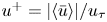 $u^{+}=|\langle \bar {u}\rangle |/u_{\tau }$ and
  $u_{\tau }=\sqrt {|\tau _{0}|/\rho }$. Wall shear stress
  $\tau _{0}$ is taken as the phase average of the total streamwise drag force acting on the wall, obtained by summation of the viscous and pressure forces divided by the area of the domain,
  $L_{x}L_{z}$. For each flow case and phase, the values of
  $k_{s}$ and
  $d'$ are optimised using an exhaustive search algorithm, taking the optimal values as those that maximise the coefficient of determination,
  $R^{2}$, between the data and (4.1) in the region
  $0\leq y\leq 0.2\delta _{{o}}$. Obtained
  $k_{s}$ and
  $d'$ values are rejected if: (a) optimised
  $R^{2}<0.98$ or (b) if they are identified as outliers according to Tukey's fences method (i.e. they fall outside the range
  $[Q_{1}-1.5(Q_{3}-Q_{1}),Q_{3}+1.5(Q_{3}-Q_{1})]$, where
  $Q_{1}$ and
  $Q_{3}$ are the lower and upper quartiles, respectively, of all obtained
  $k_{s}$ or
  $d'$ values for all flow cases and phases). The law of the wall is considered to be inapplicable at phases when obtained
  $k_{s}$ and
  $d'$ values are rejected. Representative
  $k_{s}$ and
  $d'$ values are taken as the mean of all the non-rejected values over all flow cases and phases. Taking this approach, representative
  $k_{s}=2.43$ and
  $d'=1.53$ mm, with standard deviations of 0.17 and 0.08 mm, respectively.
In terms of  $d_{50}$,
  $k_{s}=0.87d_{50}$ and
  $d'=0.54d_{50}$. These values differ from those reported in previous studies of oscillatory flow over sand or gravel beds, in which
  $k_{s}/d_{50}\approx 2\unicode{x2013}2.5$ and
  $d'/d_{50}\approx 0.15\unicode{x2013}0.35$ are typical. A likely explanation for the higher value of
  $d'/d_{50}$ than usual is that in the present study,
  $y=0$ corresponds to the vertical position of the highest roughness crest rather than a representative crest level as noted above; hence, a larger vertical shift is necessary to align the data with the zero-displacement plane. It is probable that the smaller value of
  $k_{s}/d_{50}$ than a ‘true’ sand or gravel bed results from the differences in topography. The present roughness was designed using high-resolution data obtained from an aerial scan of real gravel. In the rough wall, everything below the uppermost roughness recorded by the confocal sensor is completely impermeable, but a ‘true’ gravel bed has a degree of porosity, and hence, permeability below this level. Breugem, Boersma & Uittenbogaard (Reference Breugem, Boersma and Uittenbogaard2006) demonstrated using DNS of steady flow over walls with increasing permeability that as wall permeability increases, so does relative roughness, which corroborates the present finding.
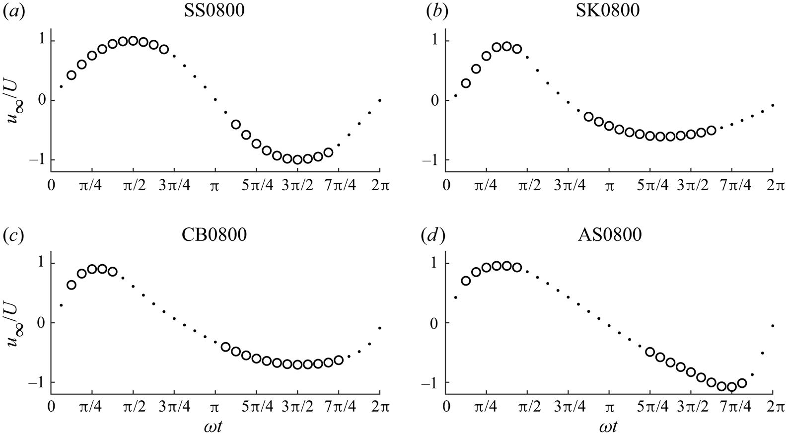
Figure 10. Free-stream velocity at 32 phases for flow cases shown above each plot (DNS data). The circles (dots) denote phases at which the law of the wall is considered applicable (inapplicable).
Flack, Schultz & Barros (Reference Flack, Schultz and Barros2020) conducted turbulent closed-channel flow experiments over roughness with variable height field standard deviation and skewness and proposed that for a rough wall with known height field statistics,  $k_{s}$ can be estimated using
 \begin{equation} k_{s}= \begin{cases} 2.73\sigma_{y}(2+{\textit{sk}}_{y})^{{-}0.45} & \text{for}\ {\textit{sk}}_{y}<0 \\ 2.11\sigma_{y} & \text{for}\ {\textit{sk}}_{y}=0 \\ 2.48\sigma_{y}(1+{\textit{sk}}_{y})^{2.24} & \text{for}\ {\textit{sk}}_{y}>0, \end{cases} \end{equation}
where  $\sigma _{y}$ and
  $ {\textit {sk}}_{y}$ are the standard deviation and skewness of the roughness height field, respectively. For the present rough wall,
  $\sigma _{y}=0.90$ mm and
  $ {\textit {sk}}_{y}=-0.63$, giving an estimated
  $k_{s}=2.13$ mm, in fairly good agreement with the obtained value of
  $k_{s}=2.43$ mm.
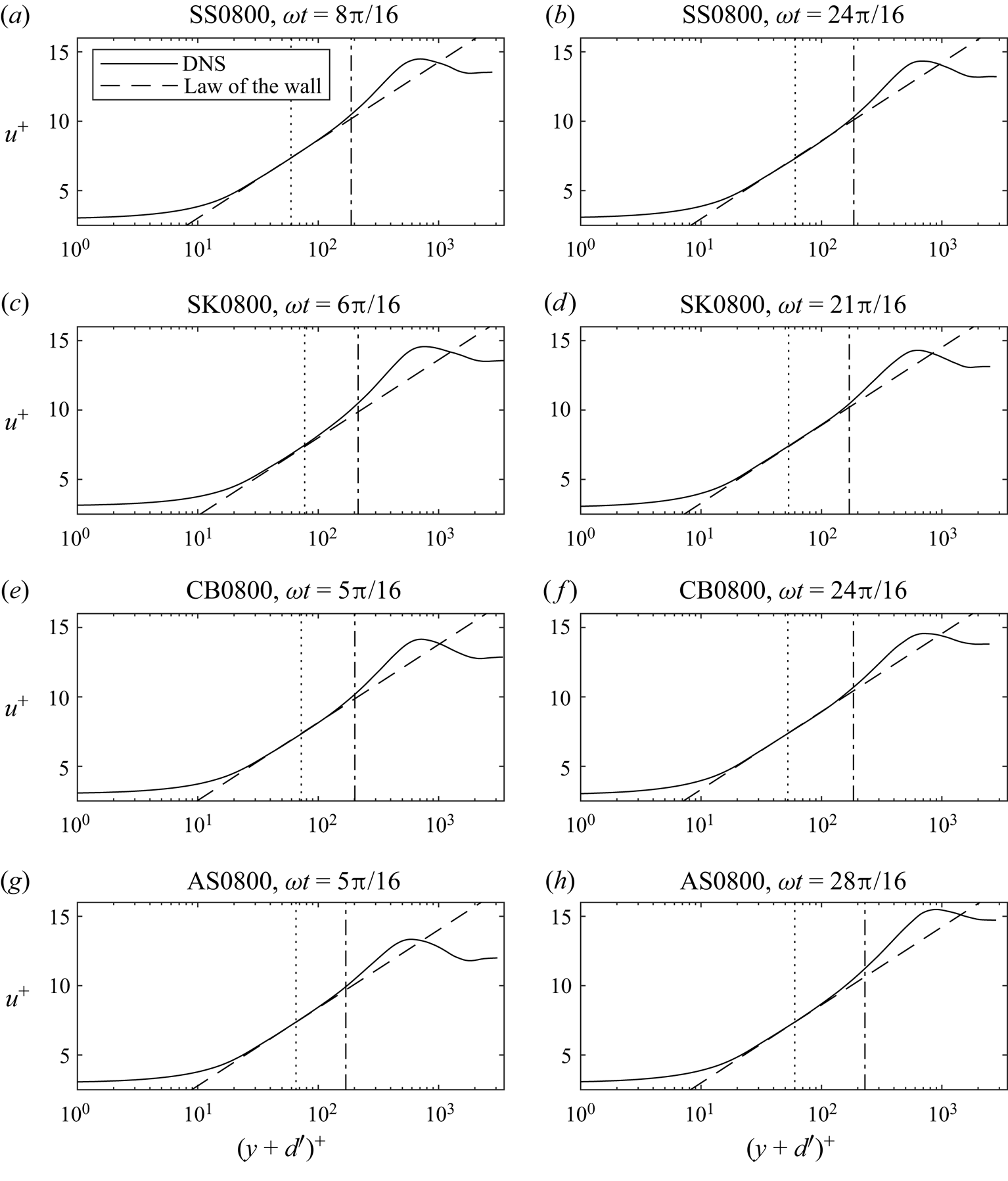
Figure 11. Comparison of the DNS data with the law of the wall, with  $k_{s}=2.43$ and
  $d'=1.53$ mm, at the phases of maximum (a,c,e,g) and minimum (b,d,f,h) free-stream velocity for each flow case. The dotted and dash-dotted lines represent
  $y=0$ and
  $y=0.2\delta _{{o}}$, respectively.
Figure 12. Boundary layer thickness as a function of  $A_{{c}}/k_{s}$ compared with previous studies. The dashed line indicates the boundary between the rough and very rough turbulent regimes.
Figure 10 illustrates the free-stream velocity for each flow case at each of the 32 phases, and shows the phases at which the law of the wall is found to be applicable. In general, the law of the wall applies during much of the accelerating phase of each half-cycle, but ceases to apply fairly early in the decelerating phase. This is in agreement with Ghodke & Apte (Reference Ghodke and Apte2016), who found that the law of the wall was applicable for  $2{\rm \pi} /10\leq t\leq 7{\rm \pi} /10$ in a DNS study of sinusoidal flow over a rough wall comprised of regularly packed spherical roughness in the very rough turbulent regime. They attributed the deviation of the velocity profile from the law of the wall at later deceleration phases to a reduction in near-roughness turbulence production resulting from the phase lead between the flow near the roughness and the free stream.
Figure 11 shows example comparisons of the DNS data with the law of the wall from (4.1), with  $k_{s}=2.43$ and
  $d'=1.53$ mm, at the phases of maximum and minimum free-stream velocity. The figure shows that there is generally good agreement between the law of the wall and the data in the region
  $0\leq y\leq 0.2\delta _{{o}}$, although for case SK0800,
  $\omega t=6{\rm \pi} /16$ and case AS0800,
  $\omega t=28{\rm \pi} /16$, the agreement is not as good. In general, the data deviate from the law of the wall at
  $y\geq 0.2\delta _{{o}}$, supporting the choice of this criterion as the upper boundary for application of the law of the wall to oscillatory flow over a rough wall. Notably, there is good agreement between the data and the law of the wall even some distance below
  $y=0$, justifying the decision to use
  $y=0$ in place of
  $y=0.2k_{s}$ as the lower boundary of the logarithmic region. The generally good agreement seen in the figure validates the representative
  $k_{s}$ and
  $d'$ values obtained from the procedure described above.
4.2. Boundary layer thickness
Figure 12 shows the ratio  $\delta _{{bl}}/k_{s}$ plotted against the inverse relative roughness
  $A/k_{s}$. Following van der A et al. (Reference van der A, O'Donoghue, Davies and Ribberink2011),
  $A_{{c}}$ is used instead of
  $A$ for the present data to account for flow asymmetry, where
  $A_{{c}}=2AT_{{ac}}/T_{{c}}$,
  $T_{{ac}}$ is the time interval from the start of the flow cycle to the time at which
  $u_{\infty }=\max (u_{\infty })$ and
  $T_{{c}}$ is the duration of the positive part of the flow cycle. The present data are compared with data from previous studies and the empirical relation given by (van der A et al. Reference van der A, O'Donoghue, Davies and Ribberink2011)
 \begin{equation} \frac{\delta_{{bl}}}{k_{s}}=0.075\left(\frac{A_{{c}}}{k_{s}}\right)^{0.82}. \end{equation}
The DNS data follow (4.5) closely, except for case SK0800 which falls below the line. This may be due to the very large value of  $ {\textit {Sk}}_{\infty }$ in this case, limiting the time available for boundary layer growth before the phase of maximum free-stream velocity is reached relative to a sinusoidal flow with comparable
  $A_{{c}}/k_{s}$. The experimental data follow the same trend as data from previous studies, although there is some variation, likely due to the relatively coarse vertical resolution high in the boundary layer, which is a consequence of the logarithmic spacing of experimental measurement positions.
4.3. Bottom phase lead
The bottom phase lead  $\phi _{0}$ is taken as the phase lead of the first harmonic of ensemble-averaged streamwise velocity between the free stream and as close to
  $y=0$ as possible. In all flow cases,
  $\phi _{0}$ is in the narrow range
  $19.7^{\circ }\leq \phi _{0}\leq 21.4^{\circ }$ for both DNS and measurements. Figure 13 shows
  $\phi _{0}$ from the present study compared with previous studies and the expression of Humbyrd (Reference Humbyrd2012) given by
 \begin{equation} \phi_{{0}}(^{{\circ}})=\frac{180}{\rm \pi}\begin{cases} \dfrac{\rm \pi}{4} & \text{for}\ 0.05\leq A_{1}/k_{s}\leq0.342 \\ -0.303\left(\dfrac{A_{1}}{k_{s}}\right)^{0.26}+0.00967 \left(\dfrac{A_{1}}{k_{s}}\right)+1.02 & \text{for}\ 0.342< A_{1}/k_{s}\leq10\\ 0.649\left(\dfrac{A_{1}}{k_{s}}\right)^{{-}0.16}+0.118 & \text{for}\ 10< A_{1}/k_{s}\leq10^{5}. \end{cases} \end{equation}
For the present data,  $A_{1}$, the orbital amplitude of the first harmonic of
  $u_{\infty }(t)$, is used in place of
  $A$. The figure shows that the present data exhibit good agreement with the trend of data from previous studies and the expression of Humbyrd (Reference Humbyrd2012).
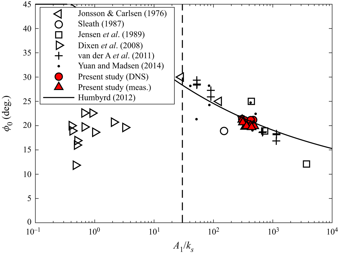
Figure 13. Bottom phase lead as a function of  $A_{1}/k_{s}$ compared with previous studies and the equation of Humbyrd (Reference Humbyrd2012). The dashed line indicates the boundary between the rough and very rough turbulent regimes.
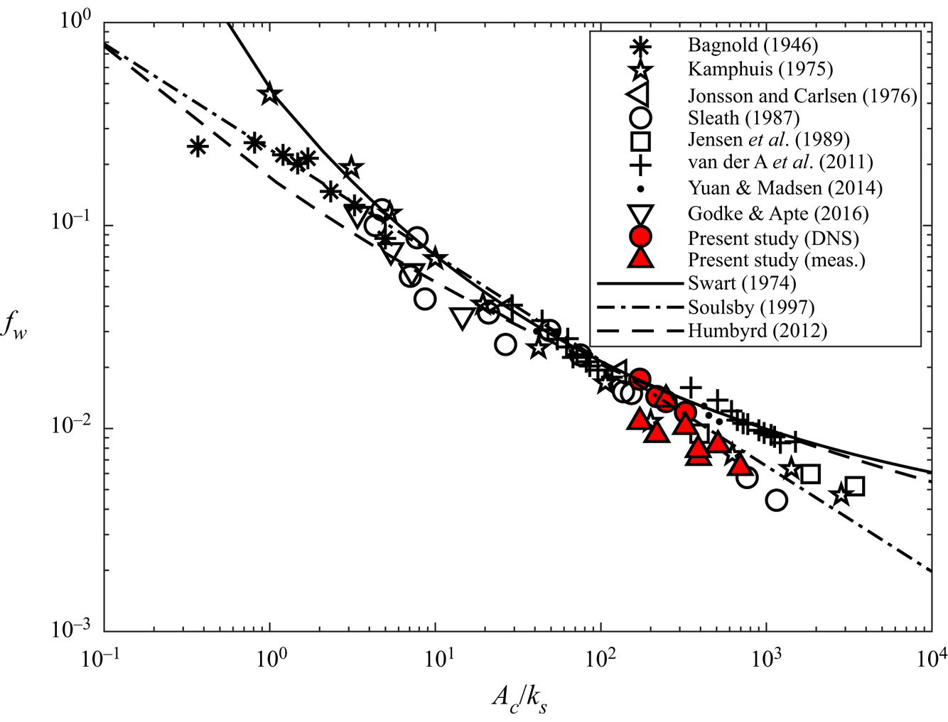
Figure 14. Value of  $f_{{w}}$ as a function of
  $A_{{c}}/k_{s}$ compared with previous studies and the equations of Swart (Reference Swart1974), Soulsby (Reference Soulsby1997) and Humbyrd (Reference Humbyrd2012).
4.4. Friction factor
Friction factor  $f_{{w}}$ is defined as
 \begin{equation} f_{{w}}=\frac{2\max[\tau_{0}(t)]}{\rho U^{2}}. \end{equation}
Experimental  $\tau _{0}(t)$ is estimated by iteratively solving (4.1)–(4.3) for
  $u_{\tau }$, which is the only unknown, since the experimental and numerical rough walls are practically identical and
  $k_{s}$ and
  $d'$ are known for the numerical roughness. This is applicable only at phases for which the law of the wall was found to apply in § 4.1. For cases with target
  $R_{\delta,\sigma }=1549$ that were not simulated using DNS, the law of the wall is assumed to apply at the same phases as the respective flow shapes for target
  $R_{\delta,\sigma }=800$. This approach is taken at all
  $y$ in the region
  $0\leq y\leq 0.2\delta _{{o}}$, with a representative
  $\tau _{0}(t)$ obtained for each phase by averaging over all applicable
  $y$ positions.
Figure 14 compares obtained friction factors with previous literature and the expressions of Swart (Reference Swart1974)
 \begin{equation} f_{{w}}=\exp\left[5.213\left(\frac{A}{k_{s}}\right)^{{-}0.194}-5.977\right], \end{equation}
Soulsby (Reference Soulsby1997):
 \begin{equation} f_{{w}}=0.237\left(\frac{A}{k_{s}}\right)^{{-}0.52}, \end{equation}
and Humbyrd (Reference Humbyrd2012)
 \begin{equation} f_{{w}}=\begin{cases} 2\left(\dfrac{30}{\kappa}\dfrac{A}{k_{s}}\right)^{-({2}/{3})} & \text{for } 0.05\leq A/k_{s}\leq0.342 \\ \exp\left[{-}1.69\left(\dfrac{A}{k_{s}}\right)^{0.344}-0.473\right]+0.0388 & \text{for }0.342< A/k_{s}\leq10\\ \exp\left[5.70\left(\dfrac{A}{k_{s}}\right)^{{-}0.101}-7.46\right] & \text{for }10< A/k_{s}\leq10^{5}. \end{cases} \end{equation}
As in figure 12,  $A_{{c}}$ is used in place of
  $A$ for the present data to account for flow asymmetry. The DNS data agree quite well with the trend of previous studies, and with the expressions of Swart (Reference Swart1974), Soulsby (Reference Soulsby1997) and Humbyrd (Reference Humbyrd2012). The experimental data fall slightly lower on the figure, but are still in good agreement with the expression of Soulsby (Reference Soulsby1997) and the experiments of Kamphuis (Reference Kamphuis1975), Sleath (Reference Sleath1987) and Jensen et al. (Reference Jensen, Sumer and Fredsøe1989).
4.5. Secondary flows
Prandtl's secondary flows of the second kind (see Nikitin, Popelenskaya & Stroh (Reference Nikitin, Popelenskaya and Stroh2021) for a review) consist of relatively low-intensity transverse motions in a flow field due to inhomogeneity in the turbulence structure. Several authors (e.g. Barros & Christensen Reference Barros and Christensen2014; Anderson et al. Reference Anderson, Barros, Christensen and Awasthi2015) observed secondary flows in wall-bounded flow over an irregular rough wall with spanwise inhomogeneity. Recently, Nikora et al. (Reference Nikora, Stoesser, Cameron, Stewart, Papadopoulos, Ouro, McSherry, Zampiron, Marusic and Falconer2019) reported the same behaviour in open-channel flow over an irregular rough wall consisting of repeating periodic elements similar to the roughness considered in the present study (it is worth noting that Barros & Christensen (Reference Barros and Christensen2014) showed that periodic roughness may induce secondary flows where non-periodic roughness may not). To date (to the authors’ knowledge), secondary flows of this type have not been reported in unsteady flows such as oscillatory flow over a rough wall.
To investigate the occurrence of secondary flows in the present study, the velocity obtained from DNS is averaged in phase and along the streamwise direction. Figure 15 shows the resulting velocity vectors (linearly interpolated onto a regular grid with spacing  ${\rm \Delta} y={\rm \Delta} z=\delta$) in the
  $y$–
$y$– $z$ plane at a selected phase for each flow condition. The figure shows clear evidence of secondary current cells, similar in appearance to those of Nikora et al. (Reference Nikora, Stoesser, Cameron, Stewart, Papadopoulos, Ouro, McSherry, Zampiron, Marusic and Falconer2019), with average spanwise spacing equal to
  $L_{z}/4$. The velocities associated with these flows are approximately two orders of magnitude smaller than
  $u_{\infty }$. Notably, the secondary flows appear weaker in magnitude in the flow cases with significant free-stream asymmetry (CB0800 and AS0800). This may be related to the shorter duration of the accelerating phase of the positive half-cycle limiting the development of the secondary flows. Due to the transient nature of oscillatory flow, the secondary flows are not present throughout the flow cycle. They start to become clearly visible near the phase of peak free-stream velocity, and are most prominent during the first half of the decelerating phase of the positive half-cycle, dissipating near the phase of flow reversal. It is notable that, for all 4 flow cases, the secondary flows appear less coherent during the second half-cycle (not shown). This is as expected for the cases with significant free-stream skewness (SK0800 and CB0800) because of the reduced velocity magnitude during the negative half-cycle, but is not expected for case SS0800 where the two half-cycles are symmetric. It is unclear if this difference in secondary flow coherence between each half-cycle is a feature of the ensemble-averaged flow or if there are simply an insufficient number of simulated flow cycles to fully resolve the secondary flows.
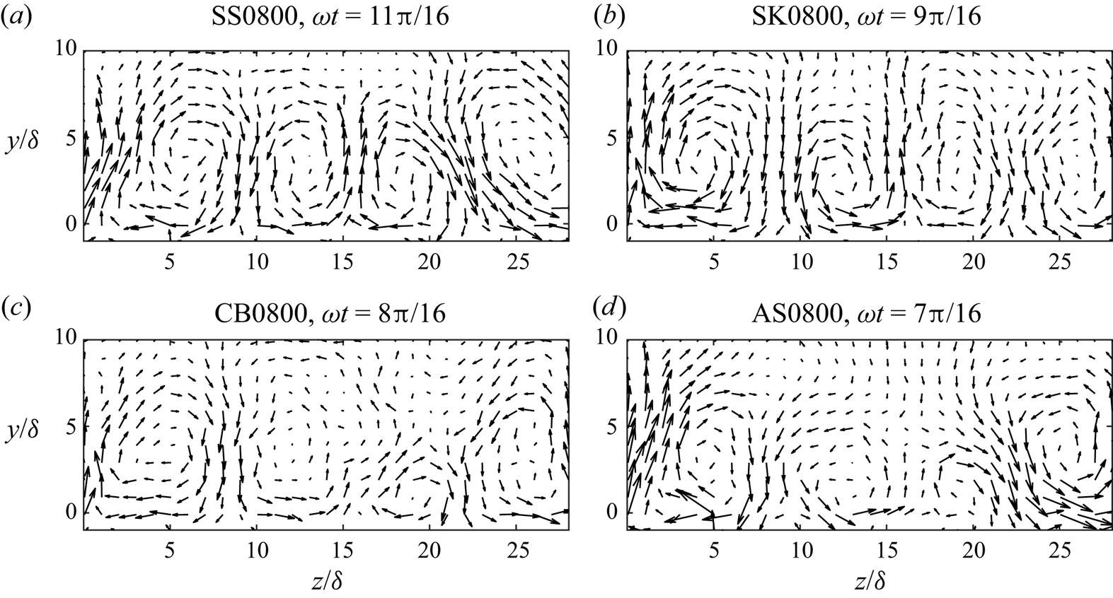
Figure 15. Velocity vectors of phase- and streamwise-averaged flow in the  $y$–
$y$– $z$ plane at the phase when secondary flows appear most prominent for each flow case (DNS data). Arrow scale:
 ![]() corresponds to
corresponds to  $\langle \bar {v}\rangle _{x}/U=0$,
  $\langle \bar {w}\rangle _{x}/U=0.02$, where angle brackets with the subscript
  $x$ denote the superficial spatial average along the streamwise direction only.
A great deal of further investigation is necessary to obtain a fundamental understanding of the secondary flows observed here. Such investigation is beyond the scope of the present study.
5. Visualisation of turbulence structure
Turbulence structure can be visualised using the isosurfaces of  $\lambda _{2}$, the second-largest eigenvalue of
  $\boldsymbol{\mathsf{S}}^{2}+{\boldsymbol{\mathsf{\Omega}}}^{2}$, where
  $\boldsymbol{\mathsf{S}}$ and
  ${\boldsymbol{\mathsf{\Omega}}}$ are the symmetric and antisymmetric parts of the velocity gradient tensor (Jeong & Hussain Reference Jeong and Hussain1995), equal to a threshold value. Vortex cores are localised in the regions characterised by
  $\lambda _{2}\leq 0$. Figure 16 shows the isosurfaces of
  $\lambda _{2}=-0.2U^{2}/\delta ^{2}$ at 8 phases during the positive half-cycle of the 10th flow cycle for case SS0800. The choice of flow cycle is arbitrary because the flow exhibits similar behaviour every cycle due to the periodicity of the driving pressure gradient and because the Reynolds number is sufficiently large for turbulence to be fully developed. The
  $\lambda _{2}$ threshold of
  $-0.2U^{2}/\delta ^{2}$ is chosen to only show the regions close to the centre of vortex cores and highlight differences in the prevalence of strong vortex structures at different phases. The figure shows that strong vortex structures aligned roughly with the streamwise coordinate are present in localised regions of the rough wall at phase
  $\omega t=2{\rm \pi} /16$. As the flow accelerates, these structures become more prevalent, emulating the dense, complex, broken structures inclined in the flow direction reported by Ghodke & Apte (Reference Ghodke and Apte2018b) for larger roughness elements at phases near maximum free-stream velocity, which suggests a significant degree of flow isotropisation in the vicinity of the roughness. It is likely that the highly irregular topology of the present rough wall contributes strongly to flow isotropisation compared with a rough wall composed of regularly arranged spheres. This is due to the chaotic nature of the flow around the dense canopy of irregularly shaped and arranged roughness elements, preventing highly coherent vortex structures from forming due to the interference of velocity fluctuations caused by the presence of nearby roughness elements.
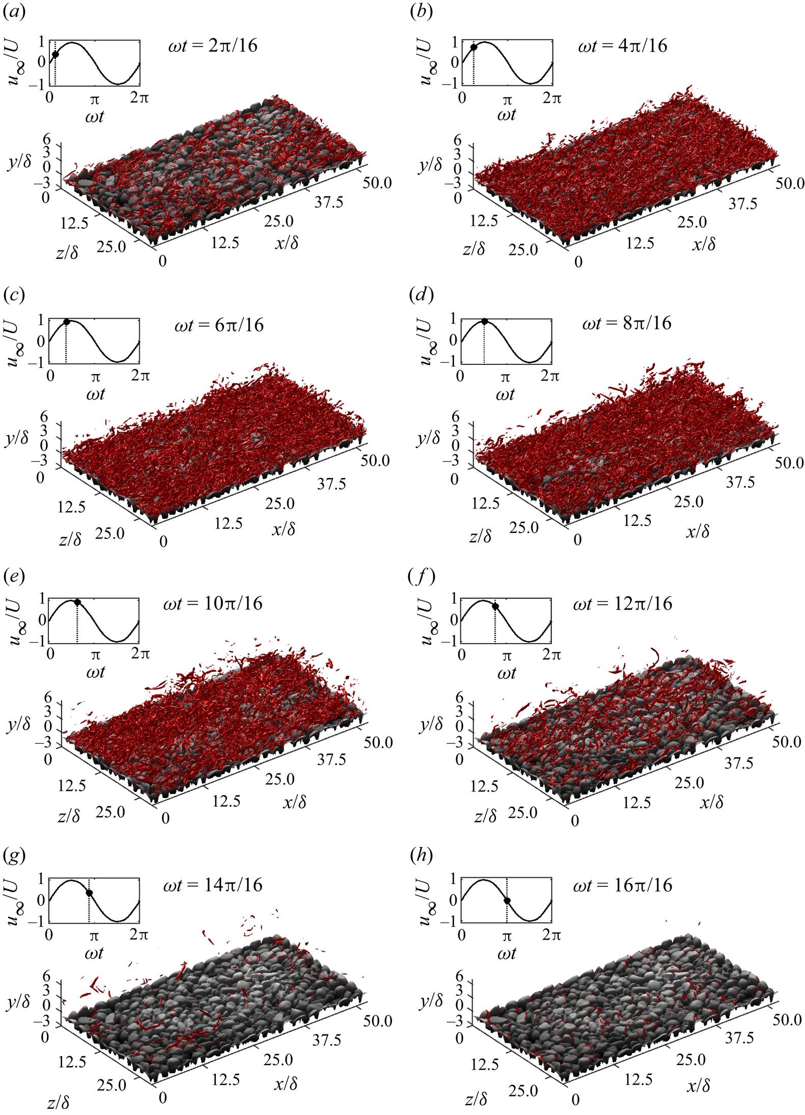
Figure 16. Isosurfaces of  $\lambda _{2}=-0.2U^{2}/\delta ^{2}$ at 8 phases during the positive half of the 10th flow cycle for case SS0800 (DNS data).
After peak free-stream velocity, the strong vortex structures become detached from the surface of the roughness and dissipate. It is notable that phases with identical free-stream velocity have very different vortex structure densities between accelerating and decelerating phases. For example, at phases  $\omega t=4{\rm \pi} /16$ and
  $\omega t=12{\rm \pi} /16$, the free-stream velocities are equal but vortex structures are much sparser at
  $\omega t=12{\rm \pi} /16$. A likely explanation for this difference is the phase lead between free-stream and near-wall velocity. This leads to a larger (smaller) near-wall velocity during accelerating (decelerating) phases corresponding to a particular value of free-stream velocity, explaining the greatly increased prevalence of strong near-wall vortex structures during acceleration phases.
While at phases close to peak free-stream velocity magnitude the turbulence is not highly structured, coherent structures are sometimes present at phases corresponding to lower free-stream velocity magnitude. For example, figure 17 shows part of the simulation domain at  $\omega t=3{\rm \pi} /16$ for case SS0800. Several coherent horseshoe structures are clearly visible that appear similar to the structures reported by Ghodke & Apte (Reference Ghodke and Apte2018b) for their small particle (SP) case. This implies that, at this phase, the near-wall turbulence is less isotropic, which is probably due to the reduced energy available for turbulence generation, resulting in less turbulent mixing. This allows some coherent structures to develop without immediately being broken by energetic velocity fluctuations.
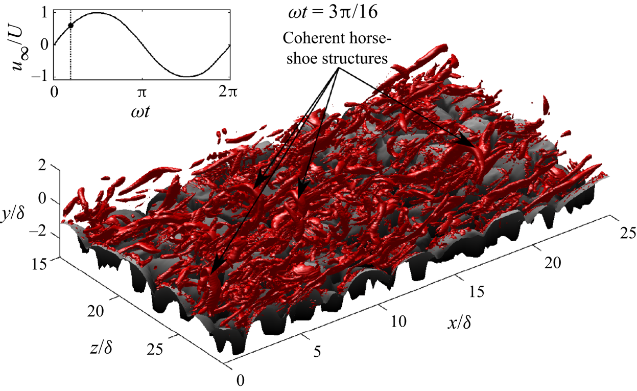
Figure 17. Isosurfaces of  $\lambda _{2}=-0.2U^{2}/\delta ^{2}$ for
  $0\leq x/\delta \leq 25$,
  $-3.1\leq y/\delta \leq 2$ and
  $15\leq z/\delta \leq 28.7$ at
  $\omega t=3{\rm \pi} /16$ for case SS0800.
Figure 18 compares the isosurfaces of  $\lambda _{2}=-0.2U^{2}/\delta ^{2}$ between the phases of maximum and minimum free-stream velocity for each flow case simulated using DNS. The figure shows that for case SS0800, the density of flow structures is similar at maximum and minimum free-stream velocity, as expected, because the two half-cycles are symmetric. However, for cases with non-zero
  $ {\textit {Sk}}_{\infty }$ or
  $ {\textit {As}}_{\infty }$, there is a significant difference in the density of strong turbulent vortices. This is most obvious for case SK0800, which is due to the large difference in maximum free-stream velocity magnitude between each half-cycle that characterises skewed flows. For case AS0800, despite maximum free-stream velocity magnitude being very similar between each half-cycle, there is still an apparent difference in vortex structure density between each half-cycle. This is caused by the higher acceleration magnitude during the accelerating phase of the positive half-cycle, which causes a larger velocity gradient, since there is less time for convection and diffusion to smooth out steep velocity gradients. This leads to faster generation of turbulence compared with the lower acceleration magnitude during the accelerating phase of the negative half-cycle. Both the skewness and asymmetry effects are present for case CB0800, but are less significant due to the smaller values of
  $ {\textit {Sk}}_{\infty }$ and
  $ {\textit {As}}_{\infty }$ compared with cases SK0800 and AS0800.
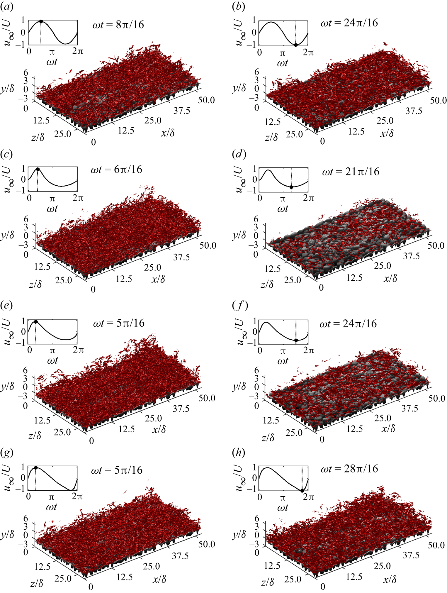
Figure 18. Isosurfaces of  $\lambda _{2}=-0.2U^{2}/\delta ^{2}$ at the phases of maximum (a,c,e,g) and minimum (b,d,f,h) free-stream velocity during the 10th flow cycle for cases (a–h) SS0800, SK0800, CB0800 and AS0800 (DNS data).
6. Momentum transfer mechanisms
6.1. Reynolds stress
Figure 19 shows vertical profiles of the normal and shear components of Reynolds stress and the shape of the Reynolds stress tensor using Lumley's triangle (Lumley & Newman (Reference Lumley and Newman1977), see figure 20 for an interpretation) at phases corresponding to flow acceleration (left), maximum free-stream velocity (middle) and deceleration (right) for each flow case simulated using DNS.
Figure 19. Vertical profiles of  $-\langle \overline {u'u'}\rangle /U^{2}$ (solid line),
  $-\langle \overline {v'v'}\rangle /U^{2}$ (dashed line),
  $-\langle \overline {w'w'}\rangle /U^{2}$ (dash-dotted line) and
  $-\langle \overline {u'v'}\rangle /U^{2}$ (dotted black line) at phases corresponding to flow acceleration (a,d,g,j), peak free-stream velocity (b,e,h,k) and deceleration (c,f,i,l) for each flow case simulated using DNS. The dotted red line denotes the vertical position of the highest roughness crest. Inset at top-left of each panel is Lumley's triangle showing the shape of the Reynolds stress tensor along
  $y$. The solid red and blue lines denote
  $y<0$ and
  $y>0$, respectively. The circle, triangle and square denote
  $y$ just above the bottom of the numerical domain, at the position of the highest roughness crest and the top of the domain, respectively.
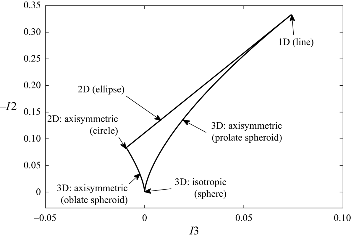
Figure 20. Lumley's triangle, with annotations showing the shape of the tensor  $\tau _{ij}$.
  $I_{2}$ and
  $I_{3}$ are the second and third invariants of
  $\tau _{ij}$, respectively. The shape of the tensor can be interpreted as follows. A spherical tensor is isotropic. A tensor with the shape of a prolate spheroid has one normal component larger than the other two, which are similar in magnitude. For a line tensor, two of the three normal components are negligible. An elliptical tensor has one negligible normal component, while the other two are dissimilar in magnitude. For a circular tensor, one normal component is negligible while the other two are similar in magnitude. A tensor with the shape of an oblate spheroid has one component smaller than the other two, which are similar in magnitude.
The figure shows that the vertical distribution of each component of Reynolds stress is similar in each flow case, exhibiting a peak just below the highest roughness crest. For all cases and phases, the streamwise component has the largest magnitude, as expected given its alignment with the flow direction, followed by the spanwise and then the wall-normal components, similar to the findings of Ghodke & Apte (Reference Ghodke and Apte2018a). The wall-normal component is smallest due to restriction of wall-normal fluctuations by the vicinity of the wall.
During flow acceleration, the peak in each Reynolds stress term is fairly sharp, becoming wider and taller at peak free-stream velocity. Once the flow begins to decelerate, the peak becomes significantly smaller in magnitude, but the layer within which the Reynolds stress is significant becomes thicker, suggesting that turbulence is convected away from the wall at these phases. This is in agreement with figure 16 at phase  $\omega t=10{\rm \pi} /16$, where some turbulent structures are observed at higher elevations than at earlier phases for case SS0800.
Figure 19 also shows that the shape of the Reynolds stress tensor is fairly two-dimensional deep inside the roughness layer (circle), where fluctuations in the streamwise and spanwise directions have similar magnitudes but wall-normal fluctuations are almost completely prevented. Note that there is some slight variation in the position of the circle within Lumley's triangle between flow cases and phases. However, at this elevation, the fluid occupies a small proportion of the overall volume, so fewer grid points are used to compute a spatial average. Hence, it is likely that this variation is due to poor convergence. In all cases, the turbulence becomes three-dimensional, taking the shape of a prolate spheroid, in the vicinity of the highest roughness crest (triangle). This shape is due to the streamwise component of Reynolds stress,  $-\langle \overline {u'u'}\rangle$, being larger in magnitude than the other two components. Far above the roughness (square), the tensor approaches a two-dimensional elliptical shape. Notably, the shape of this ellipse appears to have some dependence on flow shape, becoming more eccentric (i.e. closer to one-dimensional) for cases SS0800 and AS0800 and closer to circular for cases SK0800 and CB0800. This is because the streamwise component of Reynolds stress takes a non-zero value that appears fairly constant with
  $y$ far from the roughness, while the spanwise component decays to smaller values and the wall-normal component almost vanishes completely. The magnitude of this streamwise value is significantly larger for cases SS0800 and AS0800 compared with cases SK0800 and CB0800. A plausible explanation for this is residual turbulence from the negative half-cycle. For cases SK0800 and CB0800, the skewness of the free-stream velocity time-series results in a lower peak velocity magnitude during the negative half-cycle, resulting in a corresponding reduction in turbulence production compared with the positive half-cycle. Hence, the residual turbulence from the negative half-cycle is relatively smaller compared with cases SS0800 and AS0800, for which the peak velocity magnitude is approximately equal for both half-cycles.
The TKE, given by
 \begin{equation} \mathrm{TKE}=\tfrac{1}{2}\langle\overline{u_{i}'u_{i}'}\rangle, \end{equation}
is the energy per unit mass associated with the Reynolds stress. Figure 21 (the colour maps used for the contour plots in this article are from the ‘cmocean’ package; Thyng et al. Reference Thyng, Greene, Hetland, Zimmerle and DiMarco2016) shows the intra-period and vertical distribution of TKE for each flow case simulated using DNS. The figure shows that a burst of TKE is generated in the vicinity of the roughness during each half-cycle and is convected upwards. The dependence of TKE on flow shape is clearly visible in the figure. For case SS0800, the burst is near identical for both half-cycles, as expected given the symmetry of the flow. However, for case SK0800, large differences are apparent, with an intense but brief burst during the first half-cycle followed by a longer lasting but much less intense burst during the second half-cycle. These bursts correspond to the sharp crest and shallow trough in the free-stream velocity time series, respectively. For case AS0800, despite approximately equal peak free-stream velocity magnitude being reached in both half-cycles, differences are visible in the TKE due to the differences in free-stream acceleration. The TKE is seen to reach very large values in the vicinity of the roughness early in the first half-cycle due to the large acceleration magnitude, whereas the peak TKE occurs much later during the second half-cycle as a result of the much more gradual acceleration, and there is significant carry over of TKE from the negative half-cycle to the positive half-cycle because of the short time interval between peak negative free-stream velocity and the negative-to-positive flow reversal. Both the skewness and asymmetry effects are visible for case CB0800.
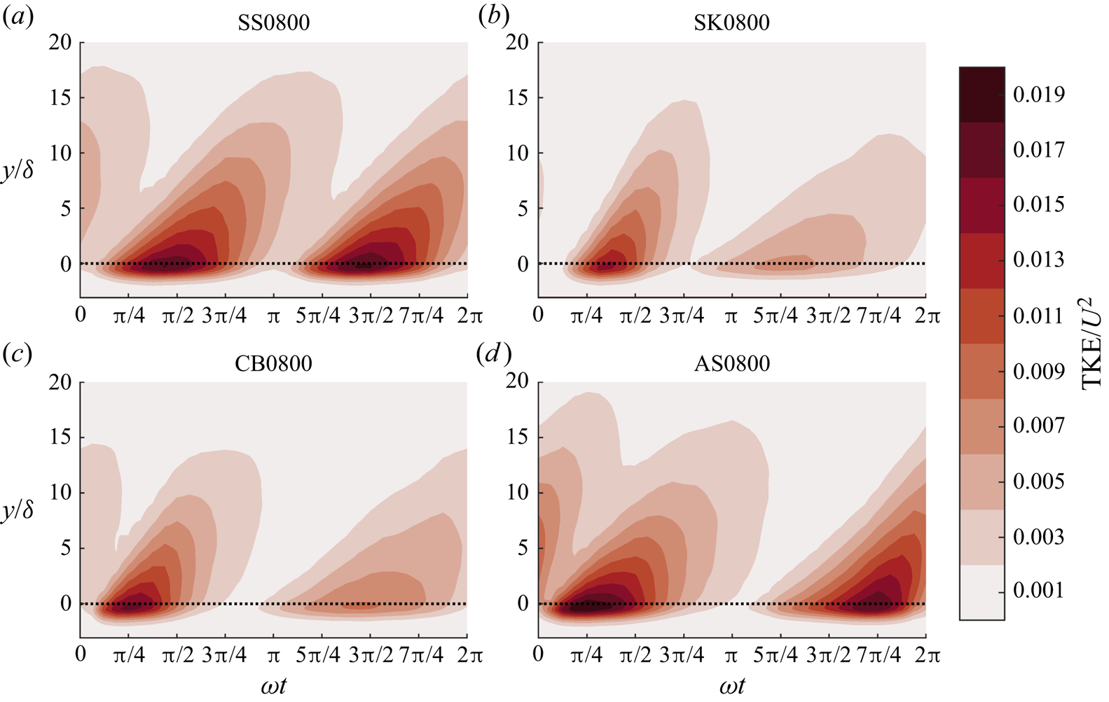
Figure 21. Intra-period and vertical distribution of TKE for each flow case simulated using DNS. The dotted line denotes the vertical position of the highest roughness crest.
6.2. Dispersive stress
Figure 22 shows vertical profiles of the normal and shear components of dispersive stress and the shape of the dispersive stress tensor using Lumley's triangle at phases corresponding to flow acceleration (a,d,j,m), maximum free-stream velocity (b,e,k,n) and deceleration (c,f,l,o) for each flow case simulated using DNS. While conventionally Lumley's triangle is used to illustrate the shape of the Reynolds stress tensor, it can be applied in a similar way to show the shape of the dispersive stress tensor. However, since the dispersive stress vanishes a short distance above the roughness, it is inappropriate to show the shape of the tensor up to the top of the domain. Hence, the shape of the tensor is shown only up to  $y=\delta _{{WKE}}$, where
  $\delta _{{WKE}}$ is defined as the vertical position at which the wake kinetic energy, given by
 \begin{equation} \mathrm{WKE}=\tfrac{1}{2}\langle\tilde{u}_{i}\tilde{u}_{i}\rangle, \end{equation}
has decayed to 0.1 % of its peak value.
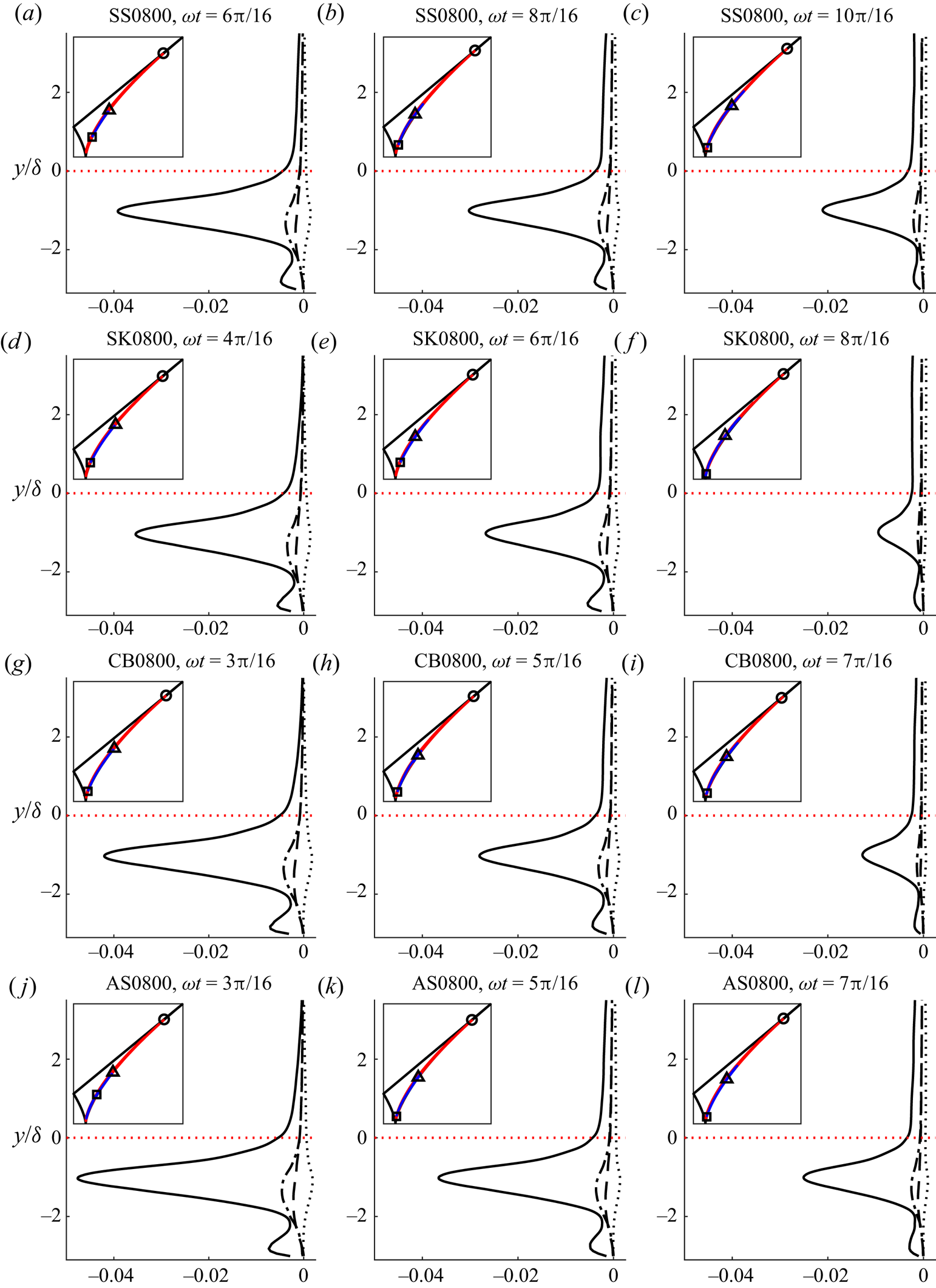
Figure 22. Vertical profiles of  $-\langle \tilde {u}\tilde {u}\rangle /U^{2}$ (solid line),
  $-\langle \tilde {v}\tilde {v}\rangle /U^{2}$ (dashed line),
  $-\langle \tilde {w}\tilde {w}\rangle /U^{2}$ (dash-dotted line) and
  $-\langle \tilde {u}\tilde {v}\rangle /U^{2}$ (dotted black line) at phases corresponding to flow acceleration (a,d,g,j), peak free-stream velocity (b,e,h,k) and deceleration (c,f,i,l) for each flow case simulated using DNS. The dotted red line denotes the vertical position of the highest roughness crest. Inset at top-left of each panel is Lumley's triangle showing the shape of the dispersive stress tensor along
  $y$. The solid red and blue lines denote
  $y<0$ and
  $y>0$, respectively. The circle, triangle and square denote
  $y$ just above the bottom of the numerical domain, at the position of the highest roughness crest and
  $y=\delta _{{WKE}}$, respectively.
Figure 23. Intra-period and vertical distribution of WKE for each flow case simulated using DNS. The dotted line denotes the vertical position of the highest roughness crest.
The region within which the dispersive stress is significant is primarily within the roughness layer, although small, rapidly decaying dispersive stresses are observed at elevations a short distance above the roughness. Similar to the Reynolds stress, the distribution of dispersive stress is comparable between each flow case, with each term exhibiting a peak at  $y/\delta \approx -1$, slightly lower than the peak in the Reynolds stress terms. The peak in the streamwise component of dispersive stress is an order of magnitude larger than the other two normal components, taking values even larger than the streamwise component of Reynolds stress. Ghodke & Apte (Reference Ghodke and Apte2018a) observed a larger discrepancy between streamwise and other normal components of dispersive stress for their SP case, which they attributed to the increased capacity of large roughness elements to redistribute energy from the streamwise direction to orthogonal directions. In the present case, roughness elements are smaller (i.e.
  $A/k_{s}$ is larger) than in both DNS cases of Ghodke & Apte (Reference Ghodke and Apte2018a), which may explain the very large discrepancy between streamwise and other normal components of dispersive stress. The spanwise peak is the second-largest, with the wall-normal dispersive stress taking very small values. This leads to a fairly insignificant dispersive shear stress despite the large magnitude of the streamwise dispersive stress.
The dispersive stresses are maximum during flow acceleration. The magnitude of dispersive stress is smaller at peak velocity magnitude and decreases further during flow deceleration, although the region within the roughness layer in which it is significant does not change substantially. However, slightly higher values of streamwise dispersive stress are seen above the roughness layer during peak velocity magnitude and flow deceleration than during acceleration. This may be due to augmented upward convection of coherent vortices at these phases.
The shape of the dispersive stress tensor appears very similar between all flow cases and phases shown in the figure. In the deep recesses of the rough wall (circle), the tensor is very close to one-dimensional, taking the shape of an eccentric prolate spheroid throughout much of the roughness layer due to the significantly larger streamwise component of dispersive stress relative to the other normal components. This eccentricity decreases towards the top of the roughness layer (triangle), with the tensor becoming closer to spherical. Above the roughness, all terms of the tensor decay to small values, resulting in the tensor becoming spherical near the vertical position at which the dispersive stress vanishes (square).
The WKE is the energy per unit mass associated with the dispersive stress. Figure 23 shows the intra-period and vertical distribution of WKE for each flow case simulated using DNS. Similar to figure 21, the figure shows a burst of WKE that is generated during each half-cycle. However, this burst is negligible above the highest roughness crest. Again, the effect of flow shape on WKE is apparent, with comparable bursts of WKE during each half-cycle for case SS0800. The effect of flow skewness and asymmetry on WKE is very similar to its effect on TKE, with a brief but intense (lingering but weak) burst of WKE generated during the first (second) half-cycle for case SK0800. For case AS0800, the peak in WKE occurs early in the first half-cycle and late in the second half-cycle, similar to the TKE. Also notable is that the peak magnitude of WKE appears much larger during the first half-cycle than the second half-cycle for case AS0800, possibly due to the very large acceleration magnitude during the accelerating phase of the first half-cycle, resulting in a larger velocity gradient. The skewness and asymmetry effects on WKE are both visible for case CB0800.
6.3. Steady streaming
A steady current is generated by non-sinusoidal turbulent OBL flow due to the non-zero time average of the Reynolds shear stress. It is worth noting that a non-zero time-averaged dispersive shear stress also contributes to the generation of this streaming in the case of non-sinusoidal oscillatory flow over a rough wall. As shown in figure 7, the steady streaming profiles differ between DNS and OFT measurements due to the boundary conditions at the ends of an OFT, generating additional streaming to balance the net flow in the OFT. Hence, here, the streaming obtained from DNS is studied in order to isolate the streaming due only to the non-zero time average of fluid shear stress.
Scandura (Reference Scandura2007) showed that the steady streaming profile in a smooth-wall OBL is given by
 \begin{equation} u_{{s}}(y)=\frac{1}{\nu}\int_{0}^{y}\overline{u'v'}_{{ta}}\,\mathrm{d}y, \end{equation}
where steady streaming  $u_{{s}}(y)$ is the time average of
  $u(y)$,
  $y=0$ corresponds to the vertical position of the smooth wall and the subscript
  $_{{ta}}$ denotes a time-averaged quantity (recall that overbar denotes a phase average; note that the phase and time averages commute). In the case of a rough-wall OBL, this equation becomes
 \begin{equation} u_{{s}}(y)=\frac{1}{\nu\phi_{s}}\int_{y_{0}}^{y}\phi_{s} \left(\langle\tilde{u}\tilde{v}\rangle_{{ta}}+\langle\overline{u'v'}\rangle_{{ta}}\right) \mathrm{d}y, \end{equation}
where  $\phi _{{s}}(y)$ is the ratio of the volume of fluid in the averaging volume to the total averaging volume and
  $y_{0}$ is the first
  $y$-position at which
  $\phi _{s}>0$. Equation (6.4) is obtained by taking the time average of the streamwise component of the double-averaged (in phase and space) Navier–Stokes equations, then taking the definite integral along
  $y$ between
  $y_{0}$ and
  $y$ twice. In the present study, the time average of the terms on the right-hand side of (6.4) could only be computed over the 32 phases at which DNS data were saved, since the terms
  $\langle \tilde {u}\tilde {v}\rangle$ and
  $\langle \overline {u'v'}\rangle$ cannot be computed until after all cycles of the simulation are completed because they require knowledge of phase-averaged quantities. Saving the necessary data to compute a satisfactory time average would require excessive data storage space. Hence the temporal resolution of the present numerical data is not sufficient to perform a satisfactory comparison between the left- and right-hand sides of (6.4).
Figure 24 shows vertical profiles of  $u_{{s}}$ computed from
  $u_{{s}}=u_{{ta}}$ for each flow case simulated using DNS. The figure shows that, as expected, the streaming is negligible for case SS0800 due to the symmetry of each half-cycle. For the three non-sinusoidal flows, a non-zero negative streaming is observed with magnitude similar to that reported by Scandura (Reference Scandura2007) for smooth-wall OBLs, extending into the free stream, where
  $u_{{s}}$ becomes approximately constant with
  $y$. An overshoot is observed in the profile for case AS0800 at
  $y/\delta \approx 12$. This overshoot suggests that the upper part of the streaming profile is not perfectly converged. A smaller overshoot is seen near
  $y/\delta =15$ for case SK0800, and no obvious overshoot is present for case CB0800. The streaming magnitude has a strong dependence on flow shape, with
  $u_{{s}}$ for case SK0800 taking values approximately double those observed for case AS0800 despite the magnitude of
  $ {\textit {Sk}}_{\infty }$ for case SK0800 and
  $ {\textit {As}}_{\infty }$ for case AS0800 being equal. This illustrates that the imbalance in fluid stress between each half-cycle is more significant for skewed flows than asymmetric flows. The magnitude of
  $u_{{s}}$ for case CB0800 is slightly larger than for case SK0800, since although
  $ {\textit {Sk}}_{\infty }$ for this case is only 71 % of
  $ {\textit {Sk}}_{\infty }$ for case SK0800, significant asymmetry is also present that contributes to the streaming.
Figure 24. Vertical profiles of steady streaming for each flow case simulated using DNS. The dotted red line denotes the vertical position of the highest roughness crest.
7. Turbulence statistics
7.1. Skewness and kurtosis of velocity fluctuations
Figure 25 shows the intra-period and vertical distribution of the skewness and kurtosis of velocity fluctuations for case SS0800. Excess kurtosis  $K_{{e},u_{i}'}=K_{u_{i}'}-3$ is shown instead of
  $K_{u_{i}'}$ because a Gaussian distribution has a kurtosis of 3.
Figure 25. Intra-period and vertical distribution of  $S_{u'}$ (a),
  $S_{v'}$ (c),
  $S_{w'}$ (e),
  $K_{{e},u'}$ (b),
  $K_{{e},v'}$ (d) and
  $K_{{e},w'}$ (f) for case SS0800. The dotted line denotes the vertical position of the highest roughness crest.
The figure shows that regions of non-Gaussian behaviour are present that originate in the vicinity of the roughness during flow reversal and acceleration for each half-cycle. At around the phase of peak free-stream velocity magnitude for each half-cycle ( $\omega t={\rm \pi} /2$ and
  $\omega t=3{\rm \pi} /2$) the turbulence statistics in the vicinity of the roughness are close to Gaussian. However, at higher elevations, the statistics are still non-Gaussian, with greater skewness and excess kurtosis magnitudes. This is because the Reynolds shear stress causes vertical convection of the non-Gaussian turbulence that is generated early in the flow cycle, resulting in the observed non-Gaussian regions moving upwards as the flow cycle progresses. The magnitudes of skewness and excess kurtosis increase at elevations further from the wall because the background turbulence level is lower at these elevations (see figure 21). Therefore, the upwardly convected turbulence represents a larger statistical deviation from the background turbulence. The decay of turbulent eddies as they are transported away from the roughness is a likely cause of the peak in
  $S_{u_{i}'}$ and
  $K_{u_{i}'}$ values that occurs at around
  $y/\delta \approx 10-20$. Some very large
  $S_{u_{i}'}$ and
  $K_{u_{i}'}$ can be seen above these elevations. However, there is very little turbulence high in the boundary layer and the higher-order statistics are unlikely to be well converged at these elevations.
Non-Gaussian behaviour can also be seen within the roughness layer. At elevations very close to the bottom of the domain, skewness and kurtosis values behave asymptotically, with magnitudes becoming large as the bottom of the domain is approached. However, in the deep recesses of the roughness that coincide with these elevations, very few grid points are inside the fluid. Hence, the intrinsic spatial average is computed over a very small number of grid points, and the statistics at these elevations cannot be considered to be well converged. Towards the top of the roughness layer, the majority of grid points are within the fluid, and the statistics can be considered to be converged to a similar degree to the statistics above the roughness layer. In this region, the magnitude of  $S_{u'}$ is relatively high, with sign equal to the sign of the free-stream velocity. This is in agreement with the near-wall statistics observed by van der A et al. (Reference van der A, Scandura and O'Donoghue2018) for oscillatory flow over a smooth wall. They attributed this to the large velocity gradient and the vicinity of the wall, since at any near-wall elevation
  $y=y_{{p}}$, fluid particles coming from
  $y>y_{{p}}$ have significantly higher velocities than particles coming from
  $y< y_{{p}}$. Hence, during the positive half-cycle, fluctuations induced by fluid particles from
  $y>y_{{p}}$ are more likely to be positive than negative, and fluctuations induced by particles from
  $y< y_{{p}}$ are more likely to be negative than positive. The vicinity of the wall means that particles below
  $y=y_{{p}}$ are restricted in the vertical distance they can travel before reaching
  $y=y_{{p}}$, but particles from
  $y>y_{{p}}$ are not subject to this restriction, and can potentially travel down from regions where
  $\langle \bar {u}\rangle$ is much higher. Hence, there is greater potential for large positive fluctuations than large negative fluctuations at
  $y=y_{p}$, resulting in a positive
  $S_{u'}$. The reverse is true during the negative half-cycle. This explanation also seems reasonable for the similar behaviour of
  $S_{u'}$ observed in the present study within the roughness layer, since the presence of roughness elements limits the potential for fluid particles to travel upwards large distances at positions close to the surface of a roughness element. Above the roughness layer, the sign of
  $S_{u'}$ in the non-Gaussian regions is opposite to that of the ensemble-averaged velocity. This is in agreement with
  $S_{u'}$ far from the wall for the turbulent channel flow study of Kim et al. (Reference Kim, Moin and Moser1987).
 $S_{v'}$ is negative throughout the flow cycle within the roughness layer. Far above the roughness,
  $S_{v'}$ is positive in the regions of non-Gaussian behaviour during both half-cycles. This behaviour begins at elevations approximately equal to the position of the highest roughness crest. Briefly existent regions of negative
  $S_{v'}$ are seen at phases close to flow reversal (
 $\omega t={\rm \pi}$ and
  $\omega t=2{\rm \pi}$). These observations are similar to the findings of van der A et al. (Reference van der A, Scandura and O'Donoghue2018) for smooth-wall oscillatory flow. They also observed positive
  $S_{v'}$ above
  $y/\delta \approx 5$, and negative
  $S_{v'}$ at
  $y/\delta \approx 1$ near flow reversal.
Notably, the magnitude of  $S_{w'}$ is insignificant throughout the flow cycle and boundary layer, the reason being that spanwise fluctuations are equally likely in either direction, since there are no asymmetries in the flow or domain in this coordinate direction. This observation is in agreement with van der A et al. (Reference van der A, Scandura and O'Donoghue2018).
The excess kurtosis of all 3 components of fluctuating velocity is seen to take large positive values within the roughness layer throughout the flow cycle. This is in contrast with van der A et al. (Reference van der A, Scandura and O'Donoghue2018), who observed very large (values up to several hundred) excess kurtosis in the vicinity of the wall that persisted only for a portion of the acceleration phase for a smooth-wall OBL. The origin of the high kurtosis in their case was streamwise-elongated streaks that formed close to the wall; once the streaks broke down due to the generation of turbulence, the kurtosis returned to much smaller values. In the present case, similar streaks cannot form near the bottom of the domain due to the presence of densely packed roughness elements. While intermittency, and therefore, large positive excess kurtosis in the smooth-wall study of van der A et al. (Reference van der A, Scandura and O'Donoghue2018) was due to streamwise streaks, in the present study the intermittency is due to the presence of the irregular roughness elements, causing large values of  $K_{u'}$,
  $K_{v'}$ and
  $K_{w'}$ that persist throughout the cycle within the roughness layer.
Figure 26 compares the intra-period and vertical distribution of the skewness and kurtosis of streamwise velocity fluctuations between each non-sinusoidal flow case simulated using DNS. Overall, the behaviour of  $S_{u'}$ and
  $K_{{e},u'}$ is very similar between the three non-sinusoidal cases and case SS0800, shown in figure 25 (similar observations can be made for the skewness and kurtosis of wall-normal and spanwise fluctuations; not shown). However, some differences are observable. Most notably,
  $S_{u'}$ is positive inside the roughness layer for a much smaller range of phases than it is negative for cases SK0800 and CB0800, in correspondence with the phases at which the free-stream velocity is positive and negative, respectively. Additionally, the phases at which the regions of non-Gaussian statistics above the roughness are initiated differ slightly, in line with the phases corresponding to flow reversal in each case. Also, the range of phases for which
  $S_{u'}$ has significant magnitude close to
  $y=0$ is wider during the second half-cycle for all three non-sinusoidal cases. This is caused by the longer time interval between flow reversal and peak free-stream velocity during the second half-cycle.
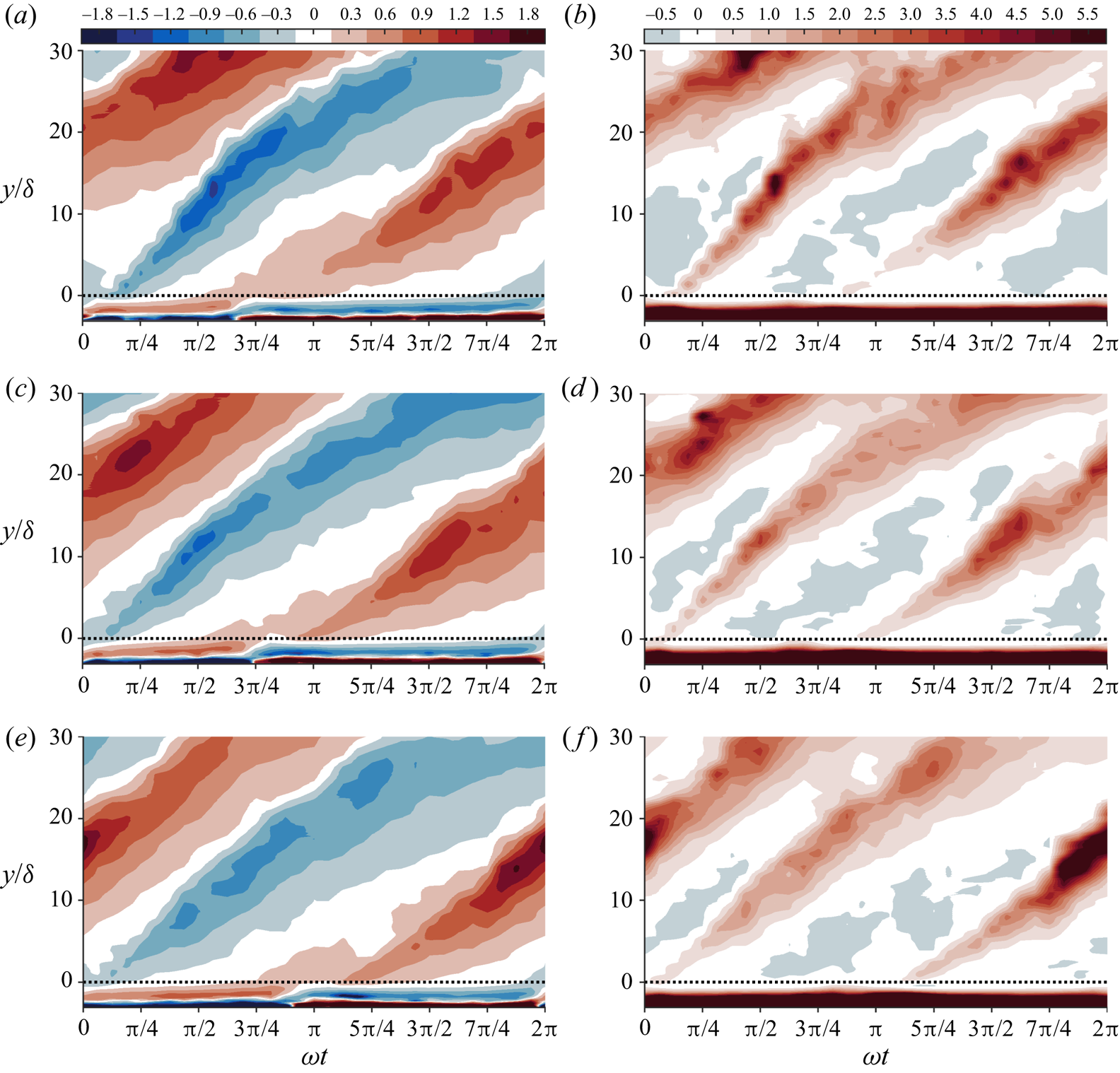
Figure 26. Intra-period and vertical distribution of  $S_{u'}$ (a,c,e) and
  $K_{{e},u'}$ (b,d,f) for case SK0800 (a,b), CB0800 (c,d) and AS0800 (e,f). The dotted line denotes the vertical position of the highest roughness crest.
The data in figures 25 and 26 suggest that a relationship exists between the skewness and kurtosis of velocity fluctuations. Figure 27 shows  $K_{u'}$ and
  $K_{v'}$ as functions of
  $S_{u'}$ and
  $S_{v'}$, respectively, for experimental and numerical data from all flow cases. Numerical data outside the range
  $-1.45< y/\delta <30$ are omitted because at
  $y/\delta <-1.45$, less than half of the grid points are within the fluid, and at
  $y/\delta >30$, there is very little turbulence. Hence, higher-order statistics are not well converged at these elevations. The figure shows that almost all the experimental and numerical data fall inside the region above the parabolas indicated by a solid line. This is in reasonable agreement with the findings of Jovanović, Durst & Johansson (Reference Jovanović, Durst and Johansson1992) and van der A et al. (Reference van der A, Scandura and O'Donoghue2018), who obtained turbulence statistics that fall inside similar parabolas for smooth-wall turbulent boundary layer flow with steady and oscillatory ensemble-averaged velocity, respectively.Of note is the non-symmetric behaviour of the data points in figure 27(b). This is because above the roughness layer,
  $S_{v'}$ is almost always positive, and has small magnitude when occasionally negative. Significant negative values of
  $S_{v'}$ are seen inside the roughness layer. However, these values are associated with very large kurtosis. Note that the data in the lower portion of the roughness layer are omitted due to poor convergence, although the asymmetry of the plotted data is retained if these values are included.
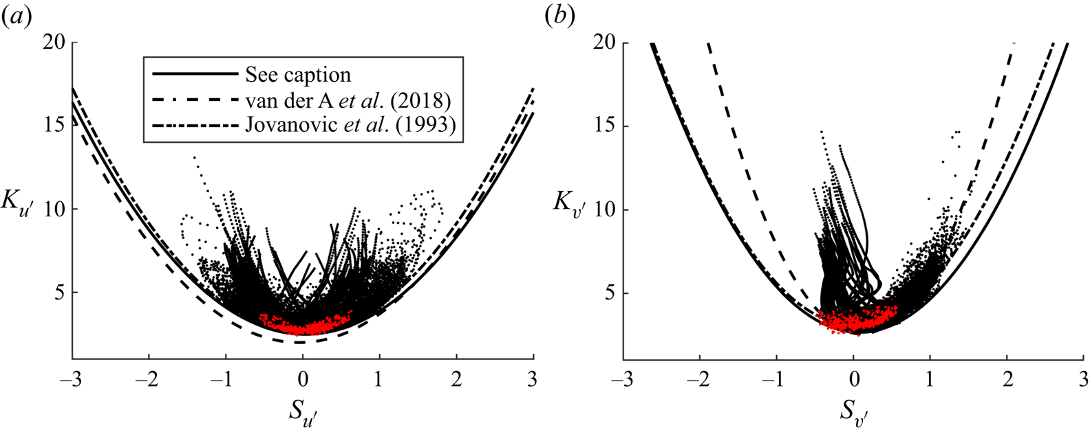
Figure 27. Relationship between  $K_{u'}$ and
  $S_{u'}$ (a) and
  $K_{v'}$ and
  $S_{v'}$ (b) for experimental data at
  $y=0.5$ and
  $y=3$ mm (red dots) for all flow conditions, and numerical data at
  $-1.45< y/\delta <30$ (black dots) for all flow conditions simulated using DNS. Equations for the parabolas indicated by the solid, dashed and dash-dotted lines are given in table 4.
Table 4. Equations for parabolas shown in figure 27.
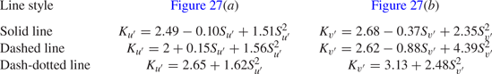
Figure 28 compares intra-period skewness and kurtosis of velocity fluctuations at  $y=3$ mm between cases AS0800 (DNS and experiment) and AS1549 (experiment only). The figure shows that the behaviour of the higher-order statistics is very similar at higher Reynolds number for the same flow shape (similar observations regarding the comparison of intra-period higher-order statistics between higher and lower Reynolds numbers can be made for the other flow shapes; not shown). However, some differences are apparent. The peaks in the magnitudes of the higher-order statistics for case AS1549 appear shifted slightly earlier in phase compared with case AS0800. This is likely due to the larger ensemble-averaged velocity magnitudes causing the initiation of new turbulence generation to occur sooner each half-cycle. The
  $S_{u'}$ values tend to be slightly closer to zero throughout the flow cycle for case AS1549 compared with case AS0800, except for a brief period after
  $S_{u'}$ crosses zero each half-cycle as a result of the faster initiation of new turbulence. Additionally, the peaks in
  $K_{u'}$ are smaller for case AS1549, and occur slightly earlier than for case AS0800. A possible reason for the peak streamwise higher-order statistic magnitudes remaining closer to Gaussian for a higher Reynolds number is that more energetic turbulence is generated during flow acceleration, increasing turbulent mixing and modulating the more extreme streamwise velocity fluctuations. Very little difference is seen in the higher-order statistics of vertical fluctuations between case AS0800 and AS1549, other than the aforementioned phase lead in the phases corresponding to peak magnitudes. Some scatter in the values of
  $K_{v'}$ is seen near
  $\omega t\approx {\rm \pi}$, but this is likely due to poorer convergence of measured statistics, since this phase coincides with flow reversal where LDA measurement reliability is lower because the rate at which seeding particles pass through the measurement volume is reduced.
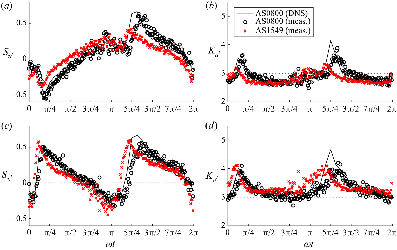
Figure 28. Comparison of streamwise and wall-normal higher-order statistics at  $y=3$ mm between cases AS0800 and AS1549. The dotted line denotes the Gaussian value of each statistic.
7.2. The PDFs of velocity fluctuations
For the practical application of the statistics of turbulence, such as the development of a stochastic sediment transport model, it is beneficial to obtain analytical expressions that describe the PDFs of the velocity fluctuations. Figures 29 and 30 show PDFs of  $u'$,
$u'$,  $v'$ and
  $w'$ normalised by their respective standard deviations for 8 phases at
  $y/\delta =1.02$ and
  $y/\delta =10.08$, respectively, for case SS0800 (similar findings are obtained for the other flow cases simulated using DNS; not shown). A total of 2.5 million data points are used to produce each histogram shown in the figure. The elevation
  $y/\delta =1.02$ is chosen because it is near the rough wall, close to where sediment transport mechanisms would be important for a mobile bed of sand or gravel, while also exhibiting noticeably non-Gaussian statistics for parts of the flow cycle. An elevation closer to
  $y=0$ is not selected because the statistics are very close to Gaussian throughout the flow cycle at
  $y=0$; see figure 25. The elevation
  $y/\delta =10.08$ is chosen because it corresponds to a vertical position where the statistics deviate more significantly from Gaussian at a wider range of phases, while still being at an elevation where TKE is significant for most of the cycle (see figure 21), ensuring that statistics are reasonably well converged.
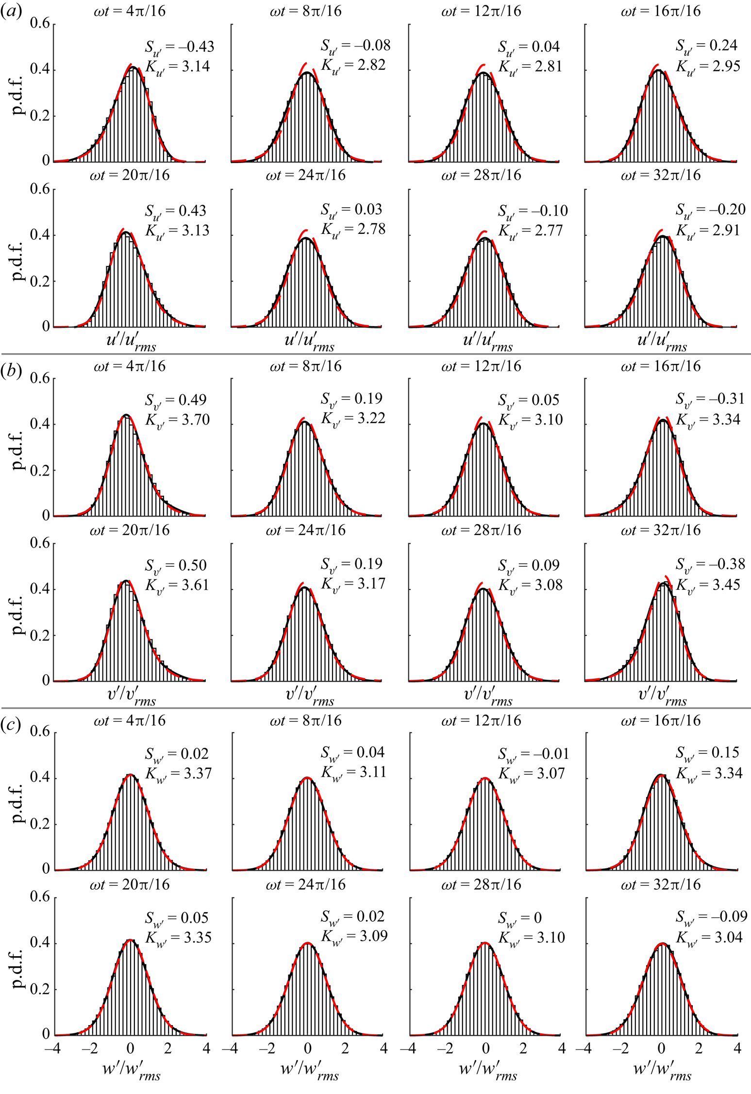
Figure 29. The PDFs of streamwise (a), wall-normal (b) and spanwise (c) velocity fluctuations normalised by their respective standard deviations for 8 phases at  $y/\delta =1.02$ for case SS0800 (DNS data). The solid black line shows the GC4 distribution, and the dashed red line shows the P4 distribution (PDFs of
  $u'/u'_{{rms}}$ and
  $v'/v'_{{rms}}$) or the P7 distribution (PDFs of
  $w'/w'_{{rms}}$).
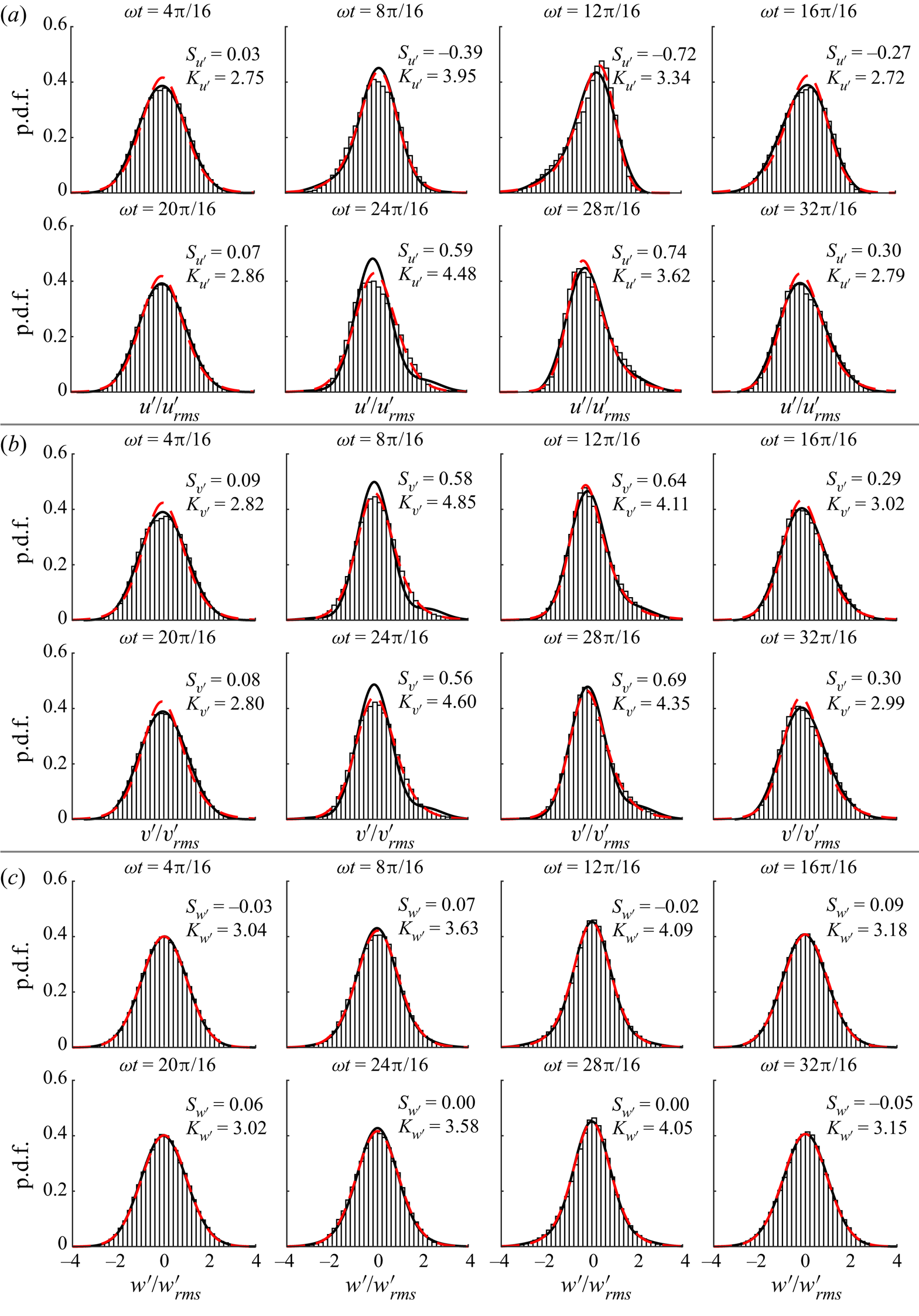
Figure 30. The PDFs of streamwise (a), wall-normal (b) and spanwise (c) velocity fluctuations normalised by their respective standard deviations for 8 phases at  $y/\delta =10.08$ for case SS0800 (DNS data). The solid black line shows the GC4 distribution, and the dashed red line shows the P4 distribution (PDFs of
  $u'/u'_{{rms}}$ and
  $v'/v'_{{rms}}$) or the P7 distribution (PDFs of
  $w'/w'_{{rms}}$).
The solid black line on the figures shows the fourth-order Gram–Charlier (GC4) distribution, given by
 \begin{equation} p_{{GC4}}(a)=\frac{\exp({-}a^{2}/2)}{\sqrt{2{\rm \pi}}}\left[1+\frac{S_{u_{i}'}}{3!}(a^3-3a)+ \frac{K_{u_{i}'}-3}{4!}(a^4-6a^2+3)\right], \end{equation}
where  $a=u_{i}'/u'_{i,{rms}}$. The GC4 distribution is convenient for practical application since it is a function of only two parameters that are equal to the skewness and kurtosis of the distribution. The red dashed line on the figures shows the Pearson type IV (P4) distribution given by
 \begin{align} p_{{P4}}(a) &= \frac{1}{b\beta_{{F}}(s-0.5,0.5)} \frac{|\varGamma_{{F}}(s+i\xi/2)|^{2}}{\varGamma_{{F}}(s)^2} \left[1+\left(\frac{a-\lambda}{b}\right)^{2}\right]^{{-}s} \nonumber\\ &\quad \times \exp\left[-\xi\tan^{{-}1}\left(\frac{a-\lambda}{b}\right)\right], \end{align}
where  $s$,
$s$,  $b$,
$b$,  $\xi$ and
  $\lambda$ are the parameters of the distribution,
  $\beta _{{F}}$ is the beta function and
  $\varGamma _{{F}}$ is the gamma function, for the PDFs of
  $u'/u_{{rms}}'$ and
  $v'/v_{{rms}}'$, and the modified Pearson type VII (P7) distribution given by
 \begin{equation} p_{{P7}}(a)=\frac{1}{\sqrt{2\gamma-3}\beta_{{F}}(\gamma-0.5,0.5)} \left[1+\left(\frac{a}{\sqrt{2\gamma-3}}\right)^{2}\right]^{-\gamma}, \end{equation}
where  $\gamma$ is the parameter of the distribution, for the PDFs of
  $w'/w_{{rms}}'$. Note that the P4 and P7 distributions are equivalent when skewness is zero, as is approximately the case for the spanwise fluctuations throughout the cycle. Additionally, as
  $\gamma \rightarrow \infty$, (7.3) approaches a Gaussian distribution. For the present data, parameters
  $s$,
$s$,  $b$,
$b$,  $\xi$,
  $\lambda$ and
  $\gamma$ in (7.2) and (7.3) are estimated using the maximum likelihood method. Figure 31 shows the variation in the parameters of the P4 and P7 distributions through the cycle at
  $y/\delta =1.02$ and
  $y/\delta =10.08$. Note that
  $\gamma$ for the P7 distribution takes very large values (up to
  $O(10^{6})$) when the PDFs are nearly Gaussian. The upper
  $y$-axis limit of 50 is applied to show the
  $\gamma$ values at phases when excess kurtosis is significant. At phases when
  $\gamma \gtrsim 50$, the PDFs can be well approximated by a Gaussian distribution.
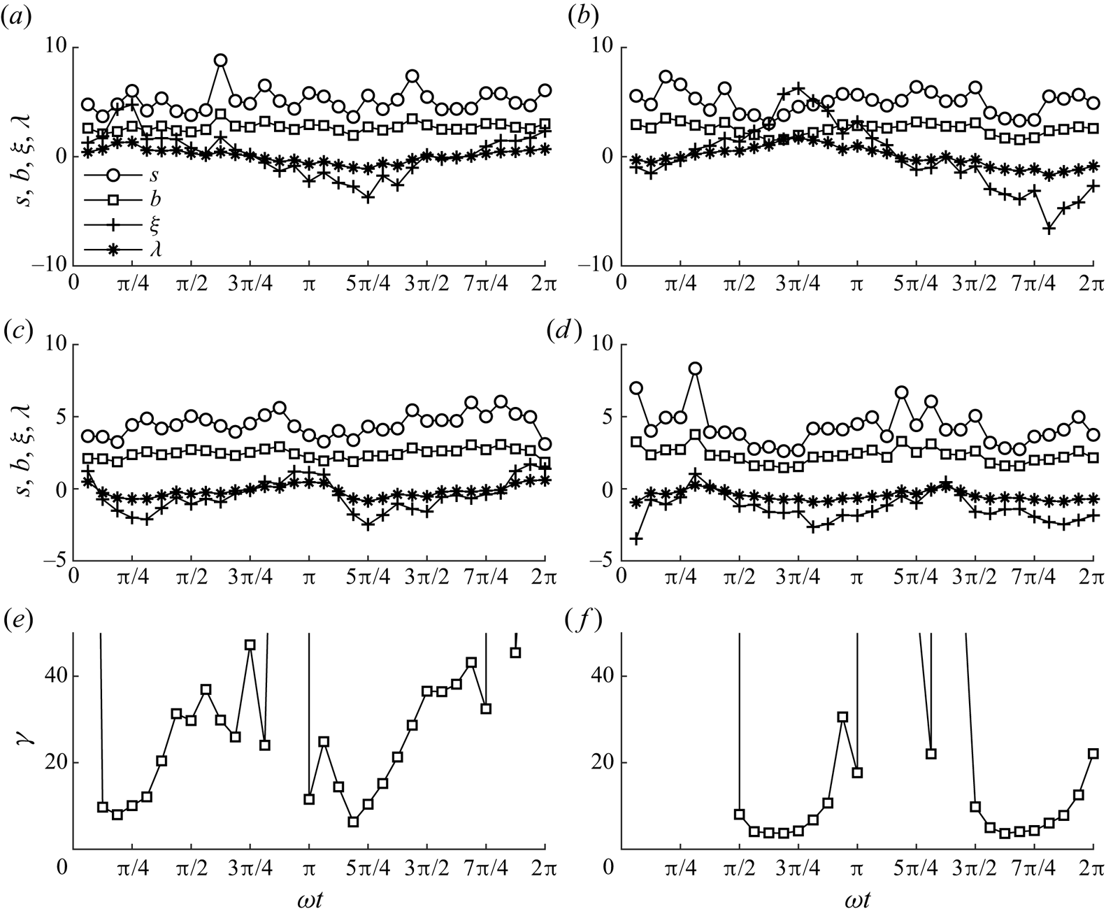
Figure 31. Intra-period variation in parameters of the Pearson distributions obtained from the maximum likelihood method for PDFs of  $u'/u'_{{rms}}$ (P4 distribution, a,b),
  $v'/v'_{{rms}}$ (P4 distribution, c,d) and
  $w'/w'_{{rms}}$ (P7 distribution, e,f) at
  $y/\delta =1.02$ (left) and
  $y/\delta =10.08$ (right) for case SS0800.
The GC4 distribution offers excellent agreement with the PDFs of all three fluctuating velocity components obtained from DNS throughout the cycle at  $y/\delta =1.02$ (see figure 29). The P4 distribution tends to slightly overestimate the peak of the PDFs of
  $u'/u'_{{rms}}$ and
  $v'/v'_{{rms}}$ but otherwise agrees well with the shape of the PDF. Very similar agreement is seen between the GC4 and P7 distributions for the PDF of
  $w'/w'_{{rms}}$. At
  $y/\delta =10.08$ (figure 30), similar observations can be made at phases when the PDFs do not deviate very significantly from Gaussian (
 $|S_{u_{i}'}|\lesssim 0.5$,
  $|K_{u_{i}'}-3|\lesssim 1.5$). However, at phases when the skewness and excess kurtosis of the fluctuations are large, e.g.
  $\omega t=24{\rm \pi} /16$, the shapes of the PDFs are better approximated by the P4 or P7 distribution compared with the GC4 distribution. In general, fair agreement is seen between the numerical PDFs and the GC4 distribution. Hence, the GC4 distribution represents a reasonable assumption for the shape of the PDF of velocity fluctuations in turbulent oscillatory flow above an irregular rough wall, and could be used as the basis for a stochastic sediment transport model in combination with empirical expressions for the skewness and kurtosis of velocity fluctuations. However, it is worth noting that the statistics investigated in the present study are averaged in space. Realistically, the pointwise statistics will vary in the vicinity of the roughness due to the inhomogeneity of the flow. For example, the skewness of fluctuations at a particular point in space close to the roughness could take a large value even if the spatially averaged skewness at the same elevation is relatively small. This effect could play an important role in sediment transport and should be the subject of future investigation.
8. Conclusion
High-precision measurements were conducted using LDA for 8 flow conditions covering 2 Reynolds numbers (taking the standard deviation of free-stream velocity as the characteristic velocity),  $R_{\delta,\sigma }=800$ and
  $R_{\delta,\sigma }=1549$, and 4 flow shapes: sinusoidal, skewed, combined (skewed and asymmetric) and asymmetric. Experimental measurements were complemented by DNS for practically identical flow conditions and roughness geometry to the 4 experimental conditions with
  $R_{\delta,\sigma }=800$. A summary of the main results is as follows:
(i) Values of equivalent sandgrain roughness length
$k_{s}$ and distance to the zero-displacement plane $d'$ obtained by comparison of the DNS data with the law of the wall are in fair agreement with the empirical expression of Flack et al. (Reference Flack, Schultz and Barros2020). In terms of $d_{50}$, obtained $k_{s}$ and $d'$ differ from values reported in previous studies of rough turbulent oscillatory flow. This is likely due to the reduced porosity of the present roughness compared with previous studies, and that the $y$-axis origin is taken to be at the level of the highest roughness crest rather than a representative crest level.(ii) Boundary layer thickness
$\delta _{{bl}}(t)$ at the phase of maximum free-stream velocity is in good agreement with previous literature in general, but falls below the trend for case SK0800, probably due to the reduced duration of the positive half-cycle, limiting time available for boundary layer growth. The maximum boundary layer thickness is found to be larger during the negative and positive half-cycle for purely skewed and asymmetric flows, respectively. The bottom phase lead $\phi _{0}$ is in the range $19.7^{\circ }\leq \phi _{0}\leq 21.4^{\circ }$ for all experimental and numerical cases and is in good agreement with the trend of previous literature and the expression of Humbyrd (Reference Humbyrd2012). Additionally, experimental and numerical friction factor $f_{{w}}$ agrees well with the trend of previous studies and the expressions of Swart (Reference Swart1974) and Humbyrd (Reference Humbyrd2012).(iii) Novel evidence of Prandtl's secondary flows of the second kind in oscillatory flows that manifest as secondary current cells with average spanwise spacing
$L_{z}/4$ is obtained. The secondary flows are transient in nature, appearing strongest during the first half of the decelerating phase of the positive half-cycle for each flow.(iv) Turbulence structures visualised using isosurfaces of the
$\lambda _{2}$ parameter at phases corresponding to peak free-stream velocity are similar to the dense, complex, broken structures inclined in the streamwise direction reported by Ghodke & Apte (Reference Ghodke and Apte2018b), suggesting significant flow isotropisation near the roughness. However, at phases corresponding to lower free-stream velocity magnitude, coherent horseshoe structures are identified, indicating a reduced degree of isotropy.(v) Of the normal components of Reynolds stress, the streamwise component is largest, followed by the spanwise and then the wall-normal components. Vertical profiles of Reynolds stress exhibit a peak just below the elevation of the highest roughness crest. The peak is sharp during flow acceleration, becoming wider and taller at peak free-stream velocity, then smaller in magnitude during flow deceleration. Similar observations are made for the vertical profiles of dispersive stress, except dispersive stress components vanish a short distance above the roughness, and the peaks occur at a slightly lower elevation of
$y/\delta \approx -1$.(vi) Using Lumley's triangle, the Reynolds stress tensor is seen to be close to circular near the bottom of the roughness layer, becoming a prolate spheroid at the top of the roughness layer, and an ellipse far above the roughness. The eccentricity of the ellipse varies between flow shapes due to the variable residual streamwise turbulence from the negative flow half-cycle. The dispersive stress tensor is nearly one-dimensional near the bottom of the roughness layer, becoming an eccentric prolate spheroid towards the top of the roughness layer that becomes increasingly circular above the roughness.
(vii) Bursts of TKE are generated each half-cycle and are convected upwards. For skewed flows, the burst is shorter but more intense during the first half-cycle, and for asymmetric flows the differences in acceleration magnitude between each half-cycle result in the peak TKE occurring earlier in the first half-cycle compared with the second half-cycle. Similar observations are made for WKE, except WKE is negligible outside the roughness layer.
(viii) A steady streaming that extends into the free-stream, similar in magnitude to the streaming observed by Scandura (Reference Scandura2007) over a smooth wall, is generated in flow cases with non-zero
$ {\textit {Sk}}_{\infty }$ and $ {\textit {As}}_{\infty }$. The streaming magnitude is largest in case CB0800, followed by case SK0800 and AS0800.(ix) Regions corresponding to non-Gaussian turbulence statistics are observed that originate near the top of the roughness layer and travel upwards, becoming further from Gaussian at higher elevations. Turbulence statistics inside the roughness layer are also observed to be highly non-Gaussian. Near the highest roughness crest, statistics are fairly close to Gaussian throughout the flow cycle.
(x) A relationship between kurtosis and skewness of velocity fluctuations similar to the relationships reported by Jovanović et al. (Reference Jovanović, Durst and Johansson1992) and van der A et al. (Reference van der A, Scandura and O'Donoghue2018) is also seen in the present study for experimental and numerical data from all flow cases.
(xi) Intra-period skewness and kurtosis of velocity fluctuations do not differ significantly between lower and higher Reynolds number, though the peaks in skewness and kurtosis of fluctuations occur earlier each half-cycle and take values closer to Gaussian when Reynolds number is larger.
(xii) The PDFs of velocity fluctuations are shown to agree reasonably closely with the GC4 distribution when
$|S_{u_{i}'}|\lesssim 0.5$, $|K_{u_{i}'}-3|\lesssim 1.5$. When statistics deviate further from Gaussian, the streamwise and wall-normal fluctuation PDFs are more closely approximated by a P4 distribution, with spanwise fluctuation PDFs better described by a P7 distribution.


Supplementary data
Further details regarding this study can be found in Dunbar (Reference Dunbar2022).
Acknowledgements
This work was conducted as part of the first author's PhD project and is also included in Dunbar (Reference Dunbar2022). The authors are grateful for the support of the technical staff at the University of Aberdeen, particularly Fluids Lab technicians R. Gillanders and J. Milne. Additionally, the authors are grateful to Dr S. Cameron and Dr M. Stewart for assistance with the design and manufacture of the experimental and numerical roughness, and Professor V. Nikora for his suggestion to look for evidence of secondary flows.
Funding
The PhD project from which this work is derived was funded by the Carnegie Trust for the Universities of Scotland (D.D., grant no. PHD00771). P.S. acknowledges the support received from the University of Catania by funding the research project ’Valutazione del rischio idraulico in sistemi complessi (VARIO)’.
Declaration of interests
The authors report no conflict of interest.
Data availability statement
The phase-averaged experimental and numerical datasets presented in this paper are openly available at https://dx.doi.org/10.5281/zenodo.7348895.


 Open access