


1. Introduction
The legitimacy of the Navier–Stokes equation is not questioned. It has a strong representativeness of real flows in many situations where the concept of the continuous medium applies. Incompressible flows, two-phase flows, variable density flows, linear waves or shock waves are all examples where the observations coincide with the solutions of the Navier–Stokes equation (Landau & Lifshitz Reference Landau and Lifshitz1959; Batchelor Reference Batchelor1967; Newton Reference Newton1990).
However, if the solutions of this equation can be qualified as conforming to reality, one can wonder about the choices that have been made for more than two centuries in the construction of this edifice that the equations of fluid mechanics represent today. Indeed, it is useful to go back to Galileo to understand the path taken by I. Newton, H. Navier, G.G. Stokes, A. Einstein and their successors in the elaboration of the laws of classical mechanics. The transposition of the theory of relativity to mechanics comes up against the necessary identification of the relationship between the velocities included in the Lorentz factor and that of the Mach number; if, for the first theory, the velocity cannot exceed the celerity of light, the passage of the threshold from a subsonic flow to a supersonic flow is a reality. In their book on fluid mechanics, Landau & Lifshitz (Reference Landau and Lifshitz1959) underline the necessity to ensure the conformity of the laws of fluid dynamics with those of special relativity. They use the quadrivector formalism of the energy-momentum tensor while keeping the concepts of classical mechanics and thermodynamics, density, pressure, and so on to obtain a wave equation after simplifications. However, attempts to render the Navier–Stokes equation relativistic in a naive way, using for that the Lorentz transformation and the classical basis of continuum mechanics, have remained unsuccessful (Geroch Reference Geroch1995; Granik & Chapline Reference Granik and Chapline1996; Wang Reference Wang2022). Finally, important questions remain, such as the existence and regularity of solutions of the Navier–Stokes equation in three space dimensions with a large time constant (Tao Reference Tao2019).
If the Navier–Stokes equation represents the most adapted and most used form to understand Newtonian viscous fluid flows, many approaches have been developed over time to find exact or approximate solutions. In fact, all the current concepts of the continuous medium type come from analytical mechanics applying the principles of differential and integral calculus developed by I. Newton and G.W. Leibniz and then by J.L. Lagrange. Discrete points of view, mimicking the properties of matter such as lattice methods of gas, lattice Boltzmann methods, close to the concepts of the kinetic theory of gases, have successfully modelled the behaviour of fluids in flow. Variational approaches are applied in the case where the Lagrangian is discontinuous (Scholle Reference Scholle2004; Scholle & Marner Reference Scholle and Marner2017; Marner et al. Reference Marner, Scholle, Herrmann and Gaskell2019); they enable us to recover the classical Navier–Stokes equations to represent incompressible and compressible flows, including shock waves. Like the stochastic variational description, these formulations remain within the context of continuum mechanics, where the quantities treated – density, momentum, energy – are those of classical mechanics.
The formalism presented in this framework is both a discrete approach, insofar as space and time are reduced to finite horizons, and a continuous approach when it reduces these quantities to zero in a homothetic way to make a differential equation appear. It is in this last sense that it can be identified as an alternative to the Navier–Stokes equation. The principle of the derivation of a new law of motion is based on the notion of conservation of integral energy, i.e. the integration on a finite length support of the intrinsic acceleration of a particle or a material medium. In classical mechanics, acceleration is considered as an ordinary quantity when it is not the derivative of velocity, itself a relative quantity. However, acceleration is considered here as an absolute quantity and it is the velocity that becomes relative by the introduction of a constant during its integration; this is not the same thing at all. Moreover, its successive derivatives have no physical interest. In Newtonian mechanics, this quantity is the ratio between force and mass, but neither of these two quantities has absolute physical meaning in the sense that they cannot be defined intrinsically. The choice of mass to describe Galileo's weak equivalence principle, where inertial mass is equal to gravitational mass, introduces a superfluous notion; indeed, this principle discussed in detail below represents only the equality of gravitational and inertial accelerations. It is this principle that will be extended in this new formulation, namely that the intrinsic acceleration of a particle or a material medium is equal to the sum of the accelerations imposed on it. Newton's second law becomes a law of conservation of acceleration. It is autonomous and does not require adjoint equations as for the Navier–Stokes equation which necessarily associates the conservation of mass equation. It is also not necessary to join an energy conservation equation because the acceleration integrated on a segment is already an expression of the mechanical energy. It does not contain any constitutive law, only the longitudinal and transverse velocities describe the physical medium.
Another pillar of the construction of discrete mechanics is based on the Helmholtz–Hodge decomposition; this orthogonal decomposition of any vector is adapted to acceleration by eliminating the harmonic component divergence-free and curl-free which makes it indeterminate for any vector in space. To eliminate this component, it is necessary to reconsider the notion of Galilean relativity, which is only related to the invariance of the equations for a constant rectilinear velocity motion by its extension to uniform expansion and rotation motions. This extended Galilean invariance then allows us to decompose the acceleration into two terms, one curl-free and the other without divergence; these are respectively the gradient of the scalar potential and the curl of the vector potential of the proper acceleration. These two potentials are energies per unit mass respectively representative of the compression and rotation effects. They are also actions in the Lagrangian sense, each being composed of a potential energy and a kinetic energy. The derivation of the law of motion is thus formed by two Lagrangians whose sum is the total energy, the integral over a segment of the acceleration. We thus directly find the three fundamental invariances of Noether's theorem: (i) time invariance; (ii) invariance by translation and (iii) invariance by rotation. Each of them corresponds to an energy conservation property. The inertia term is itself described by a Helmholtz–Hodge decomposition giving to the law of motion a great coherence and specific properties.
The new form of the law of motion is a nonlinear wave equation. The compression and rotation effects are indeed related to the longitudinal and transverse velocities in a form close to the Navier–Lamé equation. The main difference between an elastic solid and a viscous fluid is due to the absence of transverse propagation in the Newtonian fluid model. Indeed, the viscous term of the Navier–Stokes equation presents a paradox at very small time constants which is lifted if propagation is considered to replace the so-called momentum diffusion. This mechanism is replaced by a transverse propagation followed by a dissipation of energy in the form of heat. The equation of motion obtained strictly reproduces the phenomena at large time constants of the Navier–Stokes equation but lifts the paradox at small scales of time and space. From then on, this law is transformed into a wave equation whose relativistic character is easy to demonstrate. This property has become indispensable if one considers that the equation of motion harmonizes with the other laws of modern physics.
Indeed, the construction of the proposed formalism is based on the concepts introduced by Maxwell (Reference Maxwell1865) to found electromagnetism, a dynamic assembly of the laws of electrodynamics and magnetism discovered by H.C. Ørsted, A.-M. Ampère and M. Faraday; he unified these different laws by introducing a link in time. The creation of a magnetic field by a current and its reverse phenomenon are indeed due to a dynamic entanglement using intertwined circuits in the variable regime. As in electromagnetism, the compression effects in mechanics are described by a direct flow created by a pressure or scalar potential difference and the effects induced by the circulation of a flow on a closed contour surrounding the main circuit. This set can be schematized by two structures of the differential geometry, a primal structure supporting the polar vectors and a dual structure expressing the axial vectors.
The formalism adopted in this context does not deviate from those that have been developed over time in mechanics. The solutions obtained by this approach are strictly the same as those of the Navier–Stokes equation in the common ranges of their respective validities. The objective is to extend the representativeness of the laws of fluid mechanics to new constraints while respecting of course the principles of physics.
2. Main objections to the Navier–Stokes equation
The Navier–Stokes equation is the most emblematic equation in fluid mechanics. Its various formulations adapted to many fields of physics, from the notion of cosmological fluids to the study of microfluidics, have given it an undeniable status of legitimacy. However, its applications in sometimes extreme conditions lead to question the assumptions adopted for its derivation. In the same way, the progress of physics and mathematics over the last few centuries has led to the integration of certain concepts into new forms of fluid mechanics equations. This section addresses the question of the validity of certain assumptions made over time and not questioned since. To discuss these assumptions in detail, the Navier–Stokes equation is formulated in terms of a rotation equation; although this form can be found in many textbooks, it can be compared with the proposed formulation.
The equations of fluid mechanics are presented in multiple formulations depending on the problem at hand; they are often associated with energy conservation laws in one form or another, enthalpy, internal energy, entropy, etc. Let us consider one of the most classical forms, omitting the additional laws:
 \begin{equation} \left. \begin{array}{c} \displaystyle{ \rho \left( \dfrac{\partial {\boldsymbol V}}{\partial t} + {\boldsymbol V} \boldsymbol{\cdot} \boldsymbol{\nabla} {\boldsymbol V} \right) ={-} \boldsymbol{\nabla} p + \boldsymbol{\nabla} ( \lambda \boldsymbol{\nabla} \boldsymbol{\cdot} {\boldsymbol V}) + \boldsymbol{\nabla} \boldsymbol{\cdot} ( \mu ( \boldsymbol{\nabla} {\boldsymbol V} + \nabla^t {\boldsymbol V} )) } \\ \displaystyle{ \dfrac{{\rm d} \rho}{{\rm d} t} ={-} \rho \boldsymbol{\nabla} \boldsymbol{\cdot} {\boldsymbol V} } \end{array}\right\},\end{equation}
where  $\rho$ is the density, and $\lambda$ and $\mu$ the Lamé coefficients of the fluid. The adjoint law, conservation of mass, is strictly necessary; indeed, the vector Navier–Stokes equation is not self-contained even for incompressible flows. The divergence of the strain rate tensor $\boldsymbol{\mathsf{D}}$ can be developed to show the rotation rate. Since the Lamé coefficients are variable quantities depending on other quantities, the divergence of the Cauchy stress tensor is written:
 \begin{equation} \left. \begin{array}{c}
\displaystyle{ \boldsymbol{\nabla} \boldsymbol{\cdot}
\boldsymbol{\sigma} = \boldsymbol{\nabla}
\boldsymbol{\cdot} \left( - p \boldsymbol I + \lambda
\boldsymbol{\nabla} \boldsymbol{\cdot} {\boldsymbol v}
\boldsymbol I + 2 \mu \boldsymbol{\mathsf{D}} \right) } \\
\displaystyle{ \boldsymbol{\nabla} \boldsymbol{\cdot}
\boldsymbol{\sigma} ={-} \boldsymbol{\nabla} ( p - (\lambda
\!+\! 2 \mu) \boldsymbol{\nabla} \boldsymbol{\cdot}
{\boldsymbol V} ) - \mu \boldsymbol{\nabla} \!\times\!
\boldsymbol{\nabla} \!\times\! {\boldsymbol V} \!+\!
\boldsymbol{\nabla} \boldsymbol{\cdot} {\boldsymbol V}
\boldsymbol{\nabla} \lambda \!+\! \boldsymbol{\nabla} \mu
\boldsymbol{\cdot} ( \boldsymbol{\nabla} {\boldsymbol V}
+ \nabla^t {\boldsymbol V} )} \end{array}
\right\}.\end{equation}
\begin{equation} \left. \begin{array}{c}
\displaystyle{ \boldsymbol{\nabla} \boldsymbol{\cdot}
\boldsymbol{\sigma} = \boldsymbol{\nabla}
\boldsymbol{\cdot} \left( - p \boldsymbol I + \lambda
\boldsymbol{\nabla} \boldsymbol{\cdot} {\boldsymbol v}
\boldsymbol I + 2 \mu \boldsymbol{\mathsf{D}} \right) } \\
\displaystyle{ \boldsymbol{\nabla} \boldsymbol{\cdot}
\boldsymbol{\sigma} ={-} \boldsymbol{\nabla} ( p - (\lambda
\!+\! 2 \mu) \boldsymbol{\nabla} \boldsymbol{\cdot}
{\boldsymbol V} ) - \mu \boldsymbol{\nabla} \!\times\!
\boldsymbol{\nabla} \!\times\! {\boldsymbol V} \!+\!
\boldsymbol{\nabla} \boldsymbol{\cdot} {\boldsymbol V}
\boldsymbol{\nabla} \lambda \!+\! \boldsymbol{\nabla} \mu
\boldsymbol{\cdot} ( \boldsymbol{\nabla} {\boldsymbol V}
+ \nabla^t {\boldsymbol V} )} \end{array}
\right\}.\end{equation}After some rearrangements, the Navier–Stokes equation becomes
 \begin{equation} \left. \begin{array}{c}
\displaystyle{ \rho \dfrac{{\rm d} {\boldsymbol V} }{{\rm
d} t } ={-} \boldsymbol{\nabla} ( p - (\lambda \!+\! 2 \mu)
\boldsymbol{\nabla} \boldsymbol{\cdot} {\boldsymbol V} )
- \mu \boldsymbol{\nabla} \times \boldsymbol{\nabla} \times
{\boldsymbol V} \!+\! \boldsymbol{\nabla} \boldsymbol{\cdot}
{\boldsymbol V} \boldsymbol{\nabla} \lambda \!+\!
\boldsymbol{\nabla} \mu \boldsymbol{\cdot} (
\boldsymbol{\nabla} {\boldsymbol V} \!+\! \nabla^t {\boldsymbol
V} ) } \\ \displaystyle{ \dfrac{{\rm d} \rho}{{\rm d} t}
={-} \rho \boldsymbol{\nabla} \boldsymbol{\cdot}
{\boldsymbol V} } \end{array}
\right\}.\end{equation}
\begin{equation} \left. \begin{array}{c}
\displaystyle{ \rho \dfrac{{\rm d} {\boldsymbol V} }{{\rm
d} t } ={-} \boldsymbol{\nabla} ( p - (\lambda \!+\! 2 \mu)
\boldsymbol{\nabla} \boldsymbol{\cdot} {\boldsymbol V} )
- \mu \boldsymbol{\nabla} \times \boldsymbol{\nabla} \times
{\boldsymbol V} \!+\! \boldsymbol{\nabla} \boldsymbol{\cdot}
{\boldsymbol V} \boldsymbol{\nabla} \lambda \!+\!
\boldsymbol{\nabla} \mu \boldsymbol{\cdot} (
\boldsymbol{\nabla} {\boldsymbol V} \!+\! \nabla^t {\boldsymbol
V} ) } \\ \displaystyle{ \dfrac{{\rm d} \rho}{{\rm d} t}
={-} \rho \boldsymbol{\nabla} \boldsymbol{\cdot}
{\boldsymbol V} } \end{array}
\right\}.\end{equation} When the flow can be considered incompressible and with constant viscosities, i.e.  $\boldsymbol {\nabla } \boldsymbol {\cdot } {\boldsymbol V} = 0$, and $\mu = cte$ and $\lambda = cte$, (2.3) simplifies and becomes the frequently used classical form:
 \begin{equation} \left. \begin{array}{c} \displaystyle{ \rho \left( \dfrac{\partial {\boldsymbol V}}{\partial t} + \dfrac{1}{2} \boldsymbol{\nabla} ( |{\boldsymbol V} |^2 ) - {\boldsymbol V} \times \boldsymbol{\nabla} \times {\boldsymbol V} \right) ={-} \boldsymbol{\nabla} p - \boldsymbol{\nabla} \times ( \mu \boldsymbol{\nabla} \times {\boldsymbol V} )} \\ \displaystyle{ \boldsymbol{\nabla} \boldsymbol{\cdot} {\boldsymbol V} = 0 } \end{array} \right\} .\end{equation}
 The density  $\rho$ remains a variable property, for example, as a function of temperature and pressure. Whatever the methodology adopted to solve this system of equations, it is necessary to link the density and the pressure by a state law. Indeed, the number of unknowns and equations leads to close the system by a relation between these quantities. The simplification of (2.3) into (2.4) supposes that the constraint $\boldsymbol {\nabla } \boldsymbol {\cdot } {\boldsymbol V} = 0$ is guaranteed; a priori, this is not the case, it is a condition which is simply desired. In fact, it is the grouping $(\lambda + 2 \mu ) \boldsymbol {\nabla } \boldsymbol {\cdot } {\boldsymbol V}$ which must be considered because this term is of the order of magnitude of the pressure and the other terms of the equation, so the more $(\lambda + 2 \mu )$ takes important values, the more the divergence is reduced. The values of these two viscosities attributed to fluids, in particular the Stokes hypothesis, do not intrinsically ensure the incompressibility of the flow.
2.1. Stokes hypothesis
The Navier–Stokes equation for a Newtonian fluid shows the two Lamé coefficients,  $\lambda$ the compressive viscosity and $\mu$ the shear viscosity. To assign a value to $\lambda$ in the stress tensor, G.G. Stokes proposed a hypothesis linking the two Lamé coefficients in a relation $\eta = \lambda + 2/3 \mu$, where $\eta$ is named the apparent viscosity. This value of apparent viscosity is usually identified as zero and in other cases, it is the compression viscosity which is set to zero, a value obtained by solving the Boltzmann equation for monoatomic gases at very low pressure. If $\eta = 0$, the Stokes hypothesis leads to the relation $3 \lambda + 2 \mu = 0$; as $\mu$ is a positive measurable quantity, it follows that $\lambda$ can take negative values which seems unacceptable if one grants to this term the role of a viscosity. Indeed, many authors have tried to measure the value of $\lambda$ for dense gases or liquids and the values obtained are very disparate. It turns out that this assumption of Stokes is erroneous, including for monoatomic gases (Gad-El-Hak Reference Gad-El-Hak1995; Rajagopal Reference Rajagopal2013).
The Navier–Stokes equation (2.3) presents the grouping  $(\lambda + 2 \mu )$ associated with quantities related to compression such as the pressure $p$ and the divergence of the velocity $\boldsymbol {\nabla } \boldsymbol {\cdot } {\boldsymbol V}$. This grouping of the two Lamé coefficients defines a single property, compressibility or rather its inverse multiplied by a time constant $\textrm {d} t$, $\textrm {d} t/ \chi _T = (\lambda + 2 \mu )$. This expression is to be compared with the elastic coefficients of a solid where the modulus of compressional waves is equal to $M = (\lambda + 2 \mu )$, where $\lambda$ and $\mu$ are the Lamé coefficients of the elastic solid. The equivalence between fluid and solid is expressed by the displacement $\boldsymbol U = {\boldsymbol V} \, \textrm {d} t$. The isostatic modulus of elasticity $K = 1 / \chi _T$ defines in the same way the grouping $(\lambda + 2/3 \mu )$. Its perfectly measurable value for water is of the order of $K = 2 10^6 \ \textrm {Pa}$ and, as its dynamic viscosity is equal to $\mu \approx 10^{-3}$, it is easy to find $\lambda \approx K = 2 10^6 \ \textrm {Pa}$ and to see that Stokes’ law is false. Compression viscosity is the subject of numerous studies aimed at improving this notion. The one promoted by Ash, Zardadkhan & Zuckerwar (Reference Ash, Zardadkhan and Zuckerwar2011), Zuckerwar & Ash (Reference Zuckerwar and Ash2006) and Zuckerwar & Ash (Reference Zuckerwar and Ash2009) introduces two terms into the Navier–Stokes equation, the traditional volume viscosity term and a second independent term, called the pressure relaxation term; the latter term is proportional to the material time derivative of the pressure gradient. However, this approach retains the classical formalism of the Navier–Stokes equations.
By construction, there can be only two independent coefficients to represent each of the different effects, the compressive effects by the compressibility coefficient  $\chi _T$ and the shear effects by the dynamic viscosity $\mu$. The 81 coefficients of the elasticity tensor $\boldsymbol{\mathsf{C}}$ are indeed reduced to two coefficients for an isotropic fluid considering a sequence of rotations and symmetries, ${\mathsf{C}}_{12} = \lambda$ and ${\mathsf{C}}_{44} = 2 \mu$. The value of $\lambda$ is deduced from $\lambda + 2/3 \mu$ introduced in (2.1) and has strictly no influence on the behaviour of the Navier–Stokes equation; given the ratio $\mu / K \approx 10^{-3} / 10^6$, this represents a hypercompressible medium. This is the reason why the law of conservation of mass is added. It introduces in a roundabout way the real compressibility of a medium even for a gas where the ratio becomes $\mu / K \approx 10^{-5} / 10^5$ for air in normal conditions. For an isentropic flow, the determining parameter is its velocity $c_s = \sqrt {\rho \chi _s}$, where $\chi _s$ is its isentropic compressibility. In conclusion, the system (2.1) formed by the Navier–Stokes equation and its adjoint, the conservation of mass, does not require to assign a value to $\lambda$ for both compressible and incompressible flows. It should be noted that if the value of the compressional viscosity such as $\lambda = 1/ \chi _T$ were adopted in the Navier–Stokes equation (2.1), the explicit recourse to mass conservation would become unnecessary. Indeed, the operator $\boldsymbol {\nabla } ( \lambda \boldsymbol {\nabla } \boldsymbol {\cdot } {\boldsymbol V} )$ would immediately ensure the conservation of mass; in particular, a very high value of $\lambda$ would lead to implicitly impose $\boldsymbol {\nabla } \boldsymbol {\cdot } {\boldsymbol V} = 0$, the constraint which describes an incompressible flow.
2.2. Divergence and curl of material derivative
The application of the divergence and curl operators on the vector Navier–Stokes equation is particularly important because it generates second-order terms, some of which have a questionable physical meaning, especially in the case where the density is variable; this case is discarded in the remainder of this section.
The material derivative of the Navier–Stokes equation (2.1) is equal to  $\textrm {d} {\boldsymbol V} / \textrm {d} t = \partial {\boldsymbol V} / \partial t + {\boldsymbol \kappa }$, where ${\boldsymbol \kappa }$ represents the inertia; in mechanics of the continuous mediums, this is written indifferently ${\boldsymbol V} \boldsymbol {\cdot } \boldsymbol {\nabla } {\boldsymbol V}$, $\boldsymbol {\nabla } \boldsymbol {\cdot } ( {\boldsymbol V} \otimes {\boldsymbol V} ) - {\boldsymbol V} \boldsymbol {\nabla } \boldsymbol {\cdot } {\boldsymbol V}$ or $\boldsymbol {\nabla } ( | {\boldsymbol V} |^2 / 2) - {\boldsymbol V} \times \boldsymbol {\nabla } \times {\boldsymbol V}$; this last term is none other than the Lamb vector $\boldsymbol{\mathcal{L}} = - {\boldsymbol V} \times {\boldsymbol \omega }$ with ${\boldsymbol \omega } = \boldsymbol {\nabla } \times {\boldsymbol V}$, the vorticity vector. Let us consider the first term of this last form by posing $\phi _i = | {\boldsymbol V} |^2 / 2$, the inertial potential; its divergence is equal to $\boldsymbol {\nabla } \boldsymbol {\cdot } \boldsymbol {\nabla } \phi _i = \nabla ^2 \phi _i$ and its null curl, $\boldsymbol {\nabla } \times \boldsymbol {\nabla } \phi _i = 0$.
 \begin{equation} \left. \begin{array}{c}
\displaystyle{ \boldsymbol{\nabla} \boldsymbol{\cdot}
\left( \dfrac{{\rm d} {\boldsymbol V}}{{\rm d} t} \right)
\equiv \dfrac{\partial }{\partial t} \boldsymbol{\nabla}
\boldsymbol{\cdot} {\boldsymbol V} + {\boldsymbol V}
\boldsymbol{\cdot} \boldsymbol{\nabla} (
\boldsymbol{\nabla} \boldsymbol{\cdot} {\boldsymbol V} )
+ \nabla^2 \phi_i + ( \boldsymbol{\nabla}
\boldsymbol{\cdot} {\boldsymbol V} )^2 - 2 I_2 } \\
\displaystyle{ \boldsymbol{\nabla} \times \left(
\dfrac{{\rm d} {\boldsymbol V}}{{\rm d} t} \right) \equiv
\dfrac{\partial }{\partial t} \boldsymbol{\nabla} \times
{\boldsymbol V} + {\boldsymbol V} \boldsymbol{\cdot}
\boldsymbol{\nabla} ( \boldsymbol{\nabla} \times
{\boldsymbol V} ) - \boldsymbol{\nabla} \times {\boldsymbol
V} \boldsymbol{\cdot} \boldsymbol{\nabla} {\boldsymbol V}
}
\end{array}\right\},\end{equation}
\begin{equation} \left. \begin{array}{c}
\displaystyle{ \boldsymbol{\nabla} \boldsymbol{\cdot}
\left( \dfrac{{\rm d} {\boldsymbol V}}{{\rm d} t} \right)
\equiv \dfrac{\partial }{\partial t} \boldsymbol{\nabla}
\boldsymbol{\cdot} {\boldsymbol V} + {\boldsymbol V}
\boldsymbol{\cdot} \boldsymbol{\nabla} (
\boldsymbol{\nabla} \boldsymbol{\cdot} {\boldsymbol V} )
+ \nabla^2 \phi_i + ( \boldsymbol{\nabla}
\boldsymbol{\cdot} {\boldsymbol V} )^2 - 2 I_2 } \\
\displaystyle{ \boldsymbol{\nabla} \times \left(
\dfrac{{\rm d} {\boldsymbol V}}{{\rm d} t} \right) \equiv
\dfrac{\partial }{\partial t} \boldsymbol{\nabla} \times
{\boldsymbol V} + {\boldsymbol V} \boldsymbol{\cdot}
\boldsymbol{\nabla} ( \boldsymbol{\nabla} \times
{\boldsymbol V} ) - \boldsymbol{\nabla} \times {\boldsymbol
V} \boldsymbol{\cdot} \boldsymbol{\nabla} {\boldsymbol V}
}
\end{array}\right\},\end{equation}
where  $I_2$ is the second invariant of the tensor $\boldsymbol {\nabla } {\boldsymbol V}$ and where the first two terms of the right-hand members of these two relations represent respectively the material derivative of the divergence and the curl of the velocity, $\textrm {d} (\boldsymbol {\nabla } \boldsymbol {\cdot } {\boldsymbol V})/ \textrm {d} t$ and $\textrm {d} (\boldsymbol {\nabla } \times {\boldsymbol V})/ \textrm {d} t$. The divergence of the Lamb vector is composed of the flexion and enstrophy terms. These two terms are interpreted as properties of turbulent flows Hamman, Klewick & Kirby (Reference Hamman, Klewick and Kirby2008).
The first relation of (2.5) can be simplified in the case of an incompressible flow,  $\boldsymbol {\nabla } \boldsymbol {\cdot } {\boldsymbol V} = 0$; there remains the Laplacian of the scalar potential but also the second tensor invariant $\boldsymbol {\nabla } {\boldsymbol V}$. The latter is expressed by a planar surface orthogonal to the unit vector $\boldsymbol n$ of figure 2 such that $\boldsymbol n = \boldsymbol t \times \boldsymbol m$, where $\boldsymbol t$ and $\boldsymbol m$ are the unit vectors of the considered plane; if $u$ and $v$ are the components of the velocity in this plane, the term $I_2$ is the exterior product $\nabla _s u \wedge \nabla _s v$, where $s$ is the gradient operator on the considered surface. It is then possible to define a pseudo-vector $\boldsymbol{\mathcal{I}}$ whose each component would be associated with each plane of normal $\boldsymbol n$. This invariant $I_2$ has no reason to be zero even at zero divergence. This scalar is zero on the volume $\varOmega$ but not locally like the other invariants of the continuum mechanics (Tesch Reference Tesch2013). From then on, it appears that the constraint $I_2 = 0$ becomes a compatibility condition to ensure locally $\boldsymbol {\nabla } \boldsymbol {\cdot } {\boldsymbol V} = 0$ in the search for a strong solution.
The application of the curl operator to the material derivative of the velocity is written in a general way as
 \begin{equation} \boldsymbol{\nabla} \times \left( \frac{{\rm d} {\boldsymbol V}}{{\rm d} t} \right) \equiv \frac{\partial {\boldsymbol \omega} }{\partial t} + {\boldsymbol V} \boldsymbol{\cdot} \boldsymbol{\nabla} {\boldsymbol \omega} - {\boldsymbol \omega} \boldsymbol{\cdot} \boldsymbol{\nabla} {\boldsymbol V} ,\end{equation}
where  ${\boldsymbol \omega } = \boldsymbol {\nabla } \times {\boldsymbol V}$ is the vorticity vector. The first two terms of the second member represent its material derivative $\textrm {d} {\boldsymbol \omega } / \textrm {d} t$. In two dimensions of space, ${\boldsymbol V}$ and ${\boldsymbol \omega }$ are orthogonal and their scalar product is zero.
 \begin{equation} \displaystyle{ \boldsymbol{\nabla} \times \left( \frac{{\rm d} {\boldsymbol V}}{{\rm d} t} \right) \equiv \frac{\partial {\boldsymbol \omega} }{\partial t} + {\boldsymbol V} \boldsymbol{\cdot} \boldsymbol{\nabla} {\boldsymbol \omega} } .\end{equation}
 This difference between the curl of the material derivative in two and three dimensions of space is an artefact due to the vector formulation of the equations of mechanics. Indeed, the curl of velocity  $\boldsymbol {\nabla } \times {\boldsymbol V}$ is a pseudo-vector or an axial vector which has meaning only when assigned to a surface of normal $\boldsymbol n$; it is defined by Stokes’ theorem and computed on the contour of the considered surface; the vector ${\boldsymbol \omega }$ has no meaning when defined at a point in the framework of the notion of continuous medium. For an inviscid fluid, (2.6) corresponds to the conservation of vorticity.
2.3. On the origins of fictitious forces
In classical mechanics, an inertial or Galilean frame of reference corresponds to a uniform rectilinear translation at constant velocity of a body on which no action is exerted; this is the principle of inertia or Newton's first law. A rotational motion at constant velocity is considered accelerated and a rotating frame of reference is considered non-inertial.
Let us see why constant velocity rotational motion induces a fictitious force in the Navier–Stokes equation. Let us consider the rotation vector  $\boldsymbol \varOmega$, the local velocity is then equal to ${\boldsymbol V}_{rot} = \boldsymbol \varOmega \times \boldsymbol r$ and let us restrict the problem to a rotation about the axis $Oz$ such that $\omega = \boldsymbol \varOmega \boldsymbol {\cdot } \boldsymbol e_z$. The inertia term is written as either ${\boldsymbol V} \boldsymbol {\cdot } \boldsymbol {\nabla } {\boldsymbol V}$ or $\boldsymbol {\nabla } ( | {\boldsymbol V} |^2 / 2 ) - {\boldsymbol V} \times \boldsymbol {\nabla } \times {\boldsymbol V}$, where the last term is the Lamb vector $\boldsymbol{\mathcal{L}}$. In cylindrical coordinates, the only non-zero component of the Navier–Stokes equation is the one following the $r$ coordinate. Since mechanical equilibrium is not assured in an inertial reference frame, the acceleration is expressed in a rotating reference frame where the centrifugal acceleration, $- \boldsymbol \varOmega \times \boldsymbol \varOmega \times \boldsymbol r$, can be written as
 \begin{equation} {\rho \omega^2 r \boldsymbol e_r - 2 \rho \omega^2 r \boldsymbol e_r ={-} \rho \omega^2 r \boldsymbol e_r} ,\end{equation}
where the two terms on the left-hand side of (2.8) represent inertia in a Galilean reference frame and the term on the right-hand side corresponds to a fictitious centrifugal force. All the other terms, in particular the viscous terms, are zero a priori.
The necessary presence of this fictitious centrifugal force to establish mechanical equilibrium is due to the formulation of the equations of mechanics in a global Cartesian reference frame. To establish that a vector equation or vector is zero, it is necessary that all three of its components are zero simultaneously. First of all, we must notice that the equilibrium expressed by (2.8) is only supported by the following terms  $\boldsymbol e_r$. The first term is the gradient of $| {\boldsymbol V} |^2 / 2$ and the second term is also the gradient of a centrifugal potential ${\boldsymbol \omega }^2 r^2 / 2$. Therefore, the Lamb vector $\boldsymbol{\mathcal{L}} = - {\boldsymbol V} \times \boldsymbol {\nabla } \times {\boldsymbol V}$ can only be the gradient of a function of $r$ identical to the two other terms. This view of the mechanical equilibrium of a uniform rotational motion is questionable. Indeed, no constraint applies in the orthoradial direction $\boldsymbol e_{\theta }$, whereas common sense leads us to think that an acceleration along $\theta$ contributes to ensure the mechanical equilibrium.
The origin of the fictitious forces in the Navier–Stokes equation is due to the form of the apparent acceleration in the rotating reference frame which gives rise to three fictitious accelerations, the centrifugal acceleration, the Coriolis acceleration and the Euler acceleration corresponding to that of the rotating reference frame. However, it is necessary to dissociate the case of a uniform rotational motion from the problem of the change of reference frame where a velocity field is added to the local velocity of the material medium to facilitate the obtaining of solutions. One should also not confuse the dynamic actions to be performed to obtain a fixed motion with the motion itself, which is a purely kinematic view. There is no legitimate reason to consider that uniform rotational motion, with zero divergence and constant curl, is a non-inertial problem. A particle on its circular path continues its motion without bringing into play any other accelerations or forces that are specifically related to a change in direction or velocity.
The point of view developed below consists in considering that the equation of motion filters out certain uniform motions including constant velocity rotation, i.e. that it is invariant to a rotation defined by the velocity field  $\boldsymbol \varOmega \times \boldsymbol r$; this would be an extension of Galileo's principle of inertia according to which a constant velocity rotation motion continues indefinitely if it is not subjected to any external action. This is not the case for the Navier–Stokes equation, whose inertia terms generate an artefact compensated by a fictitious centrifugal force.
2.4. A non-relativistic equation
The Navier–Stokes equation is, a priori, non-relativistic. Several attempts to make this equation satisfy the Lorentz invariance remain unsuccessful for different reasons. First of all, the physical properties, the density  $\rho$, the viscosity coefficients $\lambda$ and $\mu$, make the Lorentz transformation difficult to apply. The existence of nonlinearities in the inertia terms complicates this work. Finally, the conservation of mass outside the equation itself limits the chances of simply obtaining an equation of motion that is relativistic while preserving its properties at celerities much lower than the celerity of light $c_0$.
However, the system (2.1) has a hyperbolic character because of its ability to represent longitudinal waves of celerity  $c_l$. It translates very correctly linear and nonlinear waves such as shock waves. The transposition between sound waves and light waves is not only formal; swell, acoustic and Hertzian waves are of the same nature but, of course, the propagation properties depend on the considered frequencies. One phenomenon allows us to understand the legitimacy of the comparison between acoustic waves and light waves, which is the limitation of the celerity of matter to the celerity of the medium on a straight trajectory, $c_l$ for fluids and $c_0$ for light in vacuum. In a shock tube, the solution of Euler's equation is of the form $\boldsymbol x = \pm c_l t$, where $\boldsymbol x$ is the abscissa of the wave front, and the velocity cannot exceed the celerity of sound in the fluid. The conclusions drawn by A. Einstein from the experiment of A.A. Michelson and E.W. Morlay on the non-existence of the cosmological aether at the end of the 19th century are that the speed of light is an impassable value and that it is the same in any inertial reference frame. These two observations, perfectly established in fluid mechanics and special relativity, lead to the question of a unique formalism. However, the Navier–Stokes equation is not a wave equation, even if we disregard the nonlinearity due to the inertial terms.
Another difficulty is related to viscous effects which have no equivalents in special relativity where the propagation of gravitational waves of celerity equal to  $c_0$ is of the same nature as the propagation effects of polarizable transverse waves in solid mechanics. The viscous term $\mu \nabla ^2 {\boldsymbol V}$ or its equivalent $\boldsymbol {\nabla } \times ( \mu \boldsymbol {\nabla } \times {\boldsymbol V} )$ is thus not the appropriate form to represent these transverse waves of celerity $c_t$. The Navier–Stokes equation reflects the fact that, even if these waves exist, they are instantaneously dissipated; this instantaneous character is not admissible in physics as there is always a time constant even very small which ensures the transition for the attenuation of transverse waves in viscous Newtonian fluids. The diffusion of the transverse momentum implies its dissipation. From this point of view, the phenomena of longitudinal and transverse propagation in elastic solids governed by the Navier–Lamé equation are more compatible with the relativistic formalism. Indeed, if fluid mechanics and solid mechanics are supposed to be federated within continuum mechanics, it is clear that the equations remain different.
So why is it important to look for an equation that is as representative of viscous flows as it is of light propagation? The Navier–Stokes equations have hardly evolved for more than two centuries while very important discoveries have been made in physics during this time. Maxwell's equation is relativistic and it is necessary that the equation of fluid motion be relativistic one day. Cosmology has introduced the notion of cosmological fluid by integrating the expansion of the Universe in the Euler equations. This notion of expansion is still absent from the current equations of classical mechanics where Galileo's invariance becomes insufficient. In the same way, the equivalence between mass and energy of special relativity is a pillar of physics that is neglected. The current equations of mechanics are based on the conservation of mass but also on the conservation of energy duplicated by an equation of motion which also expresses a conservation of energy. These equations are overabundant and the number of variables used is also excessive. These observations deserve special attention and a thorough examination to reduce the number of equations, variables and even the number of fundamental units in which they are expressed.
3. Principles of new formalism
3.1. Maxwell's idea
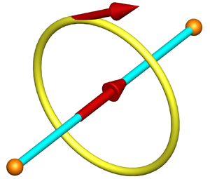
The new formalism's derivation of the law of motion is based on modelling physical phenomena in a single direction in space, that of the segment  $\varGamma$ oriented by the unit vector $\boldsymbol t$ shown in figure 1. The segment $\varGamma$, of length $\textrm {d} h$ called the discrete horizon, is bounded by two vertices $a$ and $b$. The velocity of a particle or material medium along this rectilinear segment cannot exceed the celerity $c_l$ of wave propagation in a medium, for example, the celerity $c_0$ of light in a vacuum. These elements allow us to define the time lapse $\textrm {d} t$ between the equilibrium instant $t^o$ and the current instant $t = t^o + \textrm {d} t$ by the relation $\textrm {d} h = c_l \, \textrm {d} t$. The system is in mechanical equilibrium at time $t^o$, and the law of motion predicts the solution at time $t^o + \textrm {d} t$. The quantities $\textrm {d} h$ and $\textrm {d} t$ are those that will restrict the application of the law of motion to the evolution of a physical system whose space and time scales are arbitrary. Interactions in a multi-dimensional vision of space are achieved by cause and effect, through the connection of other segments via vertices; the family of segments known as the primal structure will be denoted $\varGamma ^*$. This restriction of modelling to one dimension of space suggests the abandonment of very important notions of classical mechanics, such as one-point derivation, integration and, more generally, the abandonment of mathematical analysis.

Figure 1. Native discrete mechanics model: a rectilinear segment  $\varGamma$ of length $\textrm {d} h = [a,b]$ oriented along the unit vector $\boldsymbol t$ forms the primal structure. The dual contour $\varDelta$ positively oriented by $\boldsymbol n$ is such that $\boldsymbol t \boldsymbol {\cdot } \boldsymbol n = 0$. Acceleration $\boldsymbol \gamma$ and velocity ${\boldsymbol v}$ are vectors carried by the $\varGamma$ oriented segment; scalar potential $\phi$ is assigned to its ends and vector potential $\boldsymbol \psi$ is fixed on the $\varDelta$ contour.
The predecessors of J.C. Maxwell, of electrodynamics and magnetism, contributed with him to an exceptional discovery represented by the circulation of a direct current on a conductor  $\varGamma$ and an induced current in a loop $\varDelta$ when the regime is variable in time; the electric and magnetic fields generated by the variable currents can be reversed. Figure 1 therefore represents the dual structure $\varDelta$ oriented by the unit vector $\boldsymbol n$ such that Maxwell's corkscrew rule is respected; the unit vectors are orthogonal by construction, $\boldsymbol t \boldsymbol {\cdot } \boldsymbol n = 0$. The acceleration vectors $\boldsymbol \gamma$ and the velocity ${\boldsymbol v}$ are carried by the segment $\varGamma$, the scalars $\phi$ by the vertices of the primary structure and the pseudo-vectors $\boldsymbol \psi$ by $\boldsymbol n$.
By abandoning the global reference frame  $\mathbb {R}^3(x,y,z)$ and the notion of reference frame change, we have to build a model compatible with the local reference frame alone. This is constructed in such a way as to be able to sum the contributions of direct and induced currents on the $\varGamma$ segment alone. The direct current is produced by a potential difference between the $a$ and $b$ vertices, and the induced current on $\varGamma$ is produced, in variable regime, by the circulation of a current in the $\varDelta$ loop. The physical modelling of all phenomena is therefore performed on the $\varGamma$ segment alone. The direct effects of compression are carried by this segment in the form of the gradient of a scalar potential, and the induced effects are fixed by the dual curl of the vector potential, which projects the result onto this same segment. Each of the accelerations related to the phenomena of compression, rotation, diffusion, dissipation, gravitation, capillarity, $\ldots$ will contribute to a sum defined as a scalar on the oriented segment equal to the intrinsic acceleration of the particle or material medium under consideration.
The Maxwell-based approach to modelling all mechanical phenomena gives the discrete equation of motion very different properties from those of the Navier–Stokes equation. The latter does not propagate waves naturally, and only its combination with the continuity equation can reproduce shock waves. The discrete law of motion is intrinsically a wave equation; it possesses the attributes of a wave equation, notably that of being naturally relativistic. This quality applies not only to the propagation of light at celerity  $c_0$, but also to the propagation of any type of wave.
3.2. Primal and dual geometric structures
The control volume used by classical mechanics to derive the Navier–Stokes equation is replaced by two structures, primal and dual, illustrated in figure 2. The primary structure corresponds to the segment  $\varGamma$ with ends $a$ and $b$, and a length $\textrm {d} h = [a,b]$. This distance is called the discrete horizon, because a disturbance emitted at one end can only be felt at the other after a time $\textrm {d} t = \textrm {d} h / c_l$, where $c_l$ is the celerity of the wave in question, whether swell, sound or light. This segment is connected to other segments by their extremities, forming a family $\varGamma ^*$, which constitutes the primary mesh by flat surfaces $\mathcal {S}$ which are polygons with any number of sides. These surfaces in turn form polyhedral volumes that tessellate the entire physical domain under study. The dual structure is formed by a closed contour $\varDelta$ oriented along the vector $\boldsymbol n$ defining the facets of the dual volume $\varOmega$ whose boundaries $\partial \varOmega$ are the dual surfaces. The vectors $\boldsymbol t$ and $\boldsymbol n$, respecting Maxwell's corkscrew rule, are orthogonal by construction. Here $\varGamma$ and $\varDelta$ are contours similar to the electrical circuits of electromagnetism, including direct and induced currents.

Figure 2. Primal and dual structures mimicking the entanglement of electromagnetism between direct and induced currents; each segment  $\varGamma$ of length $\textrm {d} h = [a,b]$ is oriented by a unit vector $\boldsymbol t$. The normals to the facets $\mathcal {S}$ are also oriented along $\boldsymbol n$ with $\boldsymbol n \boldsymbol {\cdot } \boldsymbol t = 0$. The scalar potential $\phi$ is defined on each vertex of this primitive structure and the vector potential $\boldsymbol \psi$ is carried by $\boldsymbol n$. The acceleration $\boldsymbol \gamma$ and velocity ${\boldsymbol v}$ are expressed on the segment $\varGamma$, orthogonal to the dual surface $\mathcal {D}$ defined by its contour $\varDelta$.
Differential geometry allows us to establish the existence of four differential operators that exchange information between primal and dual geometric structures. The first is the discrete gradient operator,  $\boldsymbol {\nabla } \phi$, which is the restriction of the classical gradient $(\nabla ^e \phi \boldsymbol {\cdot } \boldsymbol t) \boldsymbol t$ to its only component on $\varGamma$. The primal curl operator $\boldsymbol {\nabla } \times {\boldsymbol v}$ calculated as the circulation of the vector ${\boldsymbol v}$ on the family of segments $\varGamma ^*$ projects the result onto the normal $\boldsymbol n$. The velocity divergence $\boldsymbol {\nabla } \boldsymbol {\cdot } {\boldsymbol v}$ represents the sum of fluxes across the dual surface $\mathcal {D}$, the result of which is assigned to the segment vertices. Finally, the dual curl $\boldsymbol {\nabla } \otimes \boldsymbol \psi$ is also calculated as the flux over $\varDelta$ and the result is projected onto the segment $\varGamma$. Note that the notion of tensor does not exist in discrete mechanics, and that a vector is itself a scalar assigned to an oriented segment. This allows us to unambiguously assign the symbol $\boldsymbol {\nabla } \otimes$ to the dual curl, since the tensor product no longer exists in the formalism presented. These four discrete differential operators are the only ones to describe all mechanical phenomena within a single law of motion.
The compression energy per unit mass  $\phi$ calculated from the flux through $\partial \varOmega$ by the Green–Ostrogradski theorem is assigned to the vertex $a$ of the primitive structure. The rotational energy $\boldsymbol \psi$ is calculated on the primitive facets $\mathcal {S}$ and supported by the normal $\boldsymbol n$ to them. The operator $\boldsymbol {\nabla } \phi$ represents the flow through the dual-contour facet $\varDelta$, while $\boldsymbol {\nabla } \otimes \boldsymbol \psi$ translates the flow through the primitive-contour facet $\varGamma ^*$. Both operators are carried by the single segment $\varGamma$. This formulation in potentials has multiple properties, such as $\boldsymbol {\nabla } \times \boldsymbol {\nabla } \phi = 0$ and $\boldsymbol {\nabla } \boldsymbol {\cdot } \boldsymbol {\nabla } \otimes \boldsymbol \psi = 0$, which mimic those of the continuous medium, whatever the polyhedral tessellation chosen.
The acceleration  $\boldsymbol \gamma$, a quantity considered as absolute, is associated with the segment $\varGamma$, it is both a component of the acceleration vector of space and a scalar defined on the segment oriented by $\boldsymbol t$. Similarly, the velocity vector ${\boldsymbol v}$ is a component of the vector ${\boldsymbol V}$ of space and a scalar assigned to the oriented segment $\varGamma$; but velocity, unlike acceleration, is a relative quantity whose meaning is derived from acceleration by an integration, ${\boldsymbol v} = {\boldsymbol v}^o + \boldsymbol \gamma \, \textrm {d} t$, where ${\boldsymbol v}^o$ is the velocity defined by mechanical equilibrium at time $t^o$. The current velocity ${\boldsymbol v}$ has no meaning if ${\boldsymbol v}^o$ is not fixed; it cannot therefore appear as an absolute value in an equation of motion. This condition is respected in the time derivative $\partial {\boldsymbol v} / \partial t \approx ( {\boldsymbol v} - {\boldsymbol v}^o)/ \textrm {d} t$ but must also be respected in the other terms of this equation by applying the appropriate operators.
The principle of causality is one of the pillars of discrete mechanics. This formulation suggests that the existence of two distant reference frames in which the laws of mechanics apply simultaneously is excluded. Interactions between local reference frames are only possible through a cause and effect relationship through the common vertices of the primitive structure. The only way to consider the possibility of accounting for long-distance phenomena is to define the relation between the two distant reference frames by eliminating rotational effects and using the relation  $\textrm {d} h = c_0 \, \textrm {d} t$ to account for propagation. In the case where rotational effects are present or the properties are variables, for example, the celerities $c_l$ or $c_t$, it becomes impossible to predict any motion at distance.
From a more technical point of view, the presented formulation is similar to some approaches coming from differential geometry, in particular,the methods of discrete exterior calculus (Meyer et al. Reference Meyer, Desbrun, Schröder and Barr2003; Desbrun et al. Reference Desbrun, Hirani, Leok and Marsden2005; Mohamed, Hirani & Samtaney Reference Mohamed, Hirani and Samtaney2016; Crane & Wardetzky Reference Crane and Wardetzky2018). The mimetic methods initiated by Shashkov (Reference Shashkov1996), Hyman & Shashkov (Reference Hyman and Shashkov1997) and Lipnikov, Manzini & Shashkov (Reference Lipnikov, Manzini and Shashkov2014) based on orthogonal decomposition theorems are widely used to solve Maxwell or Navier–Stokes equations.
3.3. Conservation of acceleration
The concept of momentum, sometimes presented as a principle, expresses that the material derivative of the product of mass and velocity  $\boldsymbol p = m {\boldsymbol V}$ is equal to the sum of the forces $\boldsymbol F_i$, $\textrm {d} ( m {\boldsymbol V}) / \textrm {d} t = \boldsymbol F_i$. In continuum mechanics, however, it is expressed as the product of density and velocity $\boldsymbol q = \rho {\boldsymbol V}$ and the second member becomes the sum of forces per unit volume $\boldsymbol f_i$, $\rho \, \textrm {d} {\boldsymbol V} / \textrm {d} t = \boldsymbol f_i$. The latter expression of the concept of conservation of momentum leads to the non-conservative form of the Navier–Stokes equation. In the case of variable-density flows, this introduces the difficulty of defining the density $\rho$. Whatever its form, the notion of momentum raises a major objection. In an inertial reference frame, velocity ${\boldsymbol V}$ is a relative quantity, and any constant velocity ${\boldsymbol V}_0$ is removed from the system of equations. However, this is not the case for the momentum $\boldsymbol p = m {\boldsymbol V}_0$ because $m$ can vary in time and space. The same is true for kinetic energy $E_k = m {\boldsymbol V}_0^2 / 2$. The quantities $\boldsymbol p$ and $E_k$ do not satisfy, a priori, the principle of relativity. They are even used in absolute terms to study elastic collisions between bodies, adopting the conservations of momentum $\textrm {d} \boldsymbol p / \textrm {d} t = 0$ and energy $\textrm {d} E_k / \textrm {d} t = 0$ at the instants preceding and following impact.
The principle of relativity must be applied to all quantities – velocity, of course, but also all other quantities used to describe a physical law for uniform rectilinear motion. Galilean relativity has been extended to all rotational motions (Caltagirone Reference Caltagirone2023), which means that all uniform motions can be excluded from the equation of motion. The only physical quantity that can be considered absolute is acceleration. If we denote  $\boldsymbol \gamma = \textrm {d} {\boldsymbol v} / \textrm {d} t$ the intrinsic acceleration of a body with or without mass, and $\boldsymbol h$ the sum of the accelerations applied to it, the fundamental law of dynamics can be stated as follows:
 \begin{equation} {\boldsymbol \gamma = \boldsymbol h},\end{equation}
and this law is the primary form of the equation of motion, expressed in energy per unit of mass and length.
The laws of classical mechanics are based on the conservation of mass  $m$ or density $\rho$, momentum $(\rho {\boldsymbol v})$ and energy $E$, supplemented by constitutive laws, such as a state law. They are expressed in a three-dimensional inertial reference frame $\mathbb {R}^3(x,y,z)$. In the general case, the Navier–Stokes equations have the following unknowns: (i) the three components of velocity; (ii) density; (iii) pressure and (iv) energy per unit volume $e$, i.e. six unknowns. In continuum mechanics, the number of equations must be equal to the number of unknowns: (i) the three components of the Navier–Stokes equation; (ii) the continuity equation; (iii) a state law and (iv) the energy equation.
Discrete mechanics drastically reduces the number of variables to just one, the acceleration  $\boldsymbol \gamma$, a scalar quantity attached to the segment $\gamma$. The velocity on this same segment is deduced by the relativity principle ${\boldsymbol v} = {\boldsymbol v}^o + \boldsymbol \gamma \, \textrm {d} t$, where ${\boldsymbol v}^o$ is the velocity calculated at time $t^o$. The operators divergence $\boldsymbol {\nabla } \boldsymbol {\cdot } {\boldsymbol v}$ and primal curl $\boldsymbol {\nabla } \times {\boldsymbol v}$ allow us to deduce explicitly the scalar $\phi$ and vector $\boldsymbol \psi$ potentials. The latter quantity, despite its name, is a scalar assigned to each of the oriented primal facets $\mathcal {S}$ of the normal $\boldsymbol n$. The formulation is therefore defined by the triplet $({\boldsymbol v}, \phi, \boldsymbol \psi )$ but from the acceleration $\boldsymbol \gamma$ alone. The constitutive laws as such are abandoned, and only the celerities $c_l$ and $c_t$ need to be known; these quantities are independent of the formulation. Extension to a larger dimension of space is achieved by connecting structures, an example of which is given in figure 2, through their common vertices. The interconnected segments form $\mathcal {S}$ facets of any number of sides, and these facets in turn form $\varOmega$ plane-faced polyhedra that tessellate the physical domain. The potentials $\phi ^o$ and $\boldsymbol \psi ^o$ are defined only in relation to constants. Their absolute values can only be known if their initial values at time $t = 0$ are themselves estimated. Although this is possible in some cases, these values are generally not measurable, and it is their deviation from their values at a given time $t^o$ that will enable us to predict the evolution of a system from an equation of motion. In short, the equations for conservation of momentum, mass and energy, together with a law of state, are replaced by a single law of acceleration. This drastic reduction in the number of variables and the number of unknowns is in line with the principle of parsimony, also known as Occam's razor, sometimes enunciated in physics. The term ‘razor’ refers to the distinction between two formulations leading to the same conclusions, eliminating unnecessary assumptions.
Acceleration is the total energy per unit mass and per unit length, so there is no need for another energy conservation equation. For example, heat transfer phenomena, in particular heat diffusion, will be introduced into the equation of motion itself (Caltagirone Reference Caltagirone2020a) in the form of a potential  $h = c_p T$, the enthalpy. If certain other physical phenomena are already modelled, they will be introduced in the form of specific potentials, e.g. capillary energy per unit mass, $\phi _c = \sigma \kappa$, where $\sigma$ is the surface tension per unit mass and $\kappa$ the local curvature of the interface; this potential $\phi _c$ is naturally added to the scalar potential $\phi ^o$.
The proposal formulated here is based on a return to Galileo's weak equivalence principle (WEP), which expresses the equivalence between the mass associated with gravity and that associated with the inertia of a body. This principle, taken up by I. Newton, was translated into the principle of inertia, the first law of his work. Mass appears in each of the members of his second law applied to gravitation,  $m \boldsymbol{\gamma} = m \boldsymbol g$, where $\boldsymbol \gamma$ is the acceleration of the body and $\boldsymbol g$ is the acceleration of gravity. Later, special relativity established the equivalence between mass and energy, formalized by A. Einstein's famous formula $E = m c_0^2$, where $c_0$ is the celerity of light. Despite this equivalence, the theory of special and general relativity refers to mass. This notion of mass persists to this day in many classical laws of physics. Similarly, the concept of momentum is still anchored in classical mechanics, including relativity theory, where the notions of mass and momentum are omnipresent. This concept is intimately linked to the non-acceleration of the motions it represents, and denies a priori the existence of wave propagation in the medium (swell, acoustic waves or light).
The point of view adopted revisits WEP by postulating the conservation of acceleration and therefore the conservation of energy on a segment. The law of discrete mechanics states that the acceleration of a particle or material medium is equal to the sum of the accelerations applied to it. The abandonment of other basic concepts, notably that of the global frame of reference, necessitates the creation of another geometric structure, that of a local frame of reference based on J.C. Maxwell's remarkable idea of unifying electrodynamics and magnetism (Maxwell Reference Maxwell1865).
3.4. Concept of physical homology
Mechanics has developed over time, building up a series of coherent quantities of its own. The fact that there are currently seven units to describe them in the International System of Units (SI units) shows the amount of synthesis required to achieve unification. It is therefore necessary to drastically reduce the number of these quantities. This objective is suggested by the following observation: all physical quantities that include mass in the list of units describing them, always include it in the first order, without exception. It is therefore possible to express an equivalent quantity in units of mass. For example,  $E = m c_0^2$ becomes $\phi = E / m = c_0^2$, energy per unit mass. This expression does not represent the equivalence between energy and mass; here, mass is merely a factor of proportionality. The equivalence of mass and energy is a reality, but not expressed by this formula. It is then possible to reduce the number of fundamental units for expressing the unified quantities of physics. By dividing each quantity by its mass, we deduce an equivalent quantity per unit of mass. In fact, only two fundamental units are needed to describe the unified quantities: length and time, the SI system's metres and seconds.
Analysis of the mechanical phenomena associated with the reference frame of figure 1 leads to a minimal number of fundamental variables: (i) the acceleration  $\boldsymbol \gamma$ and velocity ${\boldsymbol v}$ of the fluid on $\varGamma$; (ii) the scalar potential $\phi$, an energy per unit mass and (iii) the vector potential $\boldsymbol \psi$, also an energy per unit mass. Two other quantities represent fundamental physical characteristics: longitudinal velocity $c_l$ and transverse velocity $c_t$. These two quantities are properties of the medium and will not be modelled; they will simply be known and may depend on the other fundamental variables. The variables $({\boldsymbol v}, \phi, \boldsymbol \psi )$ and the properties of the media $(c_l, c_t)$ are the only quantities necessary and sufficient to model all physical phenomena for the classical fields of mechanics. All these quantities can only be expressed in two fundamental units: length and time. This reduction of mechanical quantities and units opens the way to possible analogies between apparently different phenomena.
Let us look at a few phenomena that are a priori disjoint in classical physics. To begin with, let us consider the velocity of the photon compared with the celerity limitation of a fluid in a pipe, the phenomenon of sonic blockage. Experiments by Michelson & Morley (Reference Michelson and Morley1887) show that the celerity of light in vacuum  $c_0$ is invariant with respect to the direction of propagation. Light is represented both as a wave and as massless particles, the photons, which have a priori a velocity equal to the celerity $c_0$. Consider a gas injected into a tube of constant cross-section from a converging channel; the velocity of the gas increases in the converging channel, but is limited in the tube by the local celerity $c_l$, whatever the pressure difference maintained between upstream and downstream of the tube. This phenomenon of sonic blockage is well explained by Hugoniot's theorem, established in the 19th century. So, in the case of directional motion, the particles – photon or gas – are limited to a velocity equal to the celerity of the medium. Other considerations concerning the need for a material medium for sound propagation in gases are linked to the very different orders of magnitude of wave propagation celerities in the two media. The solutions of the mechanical equations, Euler or Navier–Stokes, and the results of special relativity that lead to the phenomenon of sound blocking are the same. The result obtained in discrete mechanics (Caltagirone Reference Caltagirone2023) for a uniformly accelerated particle whose velocity is limited by the celerity of the medium is also consistent with those of the first formulations. These phenomena belong to the same physics as homology.
3.5. Mass-energy equivalence
The equivalence between mass and energy is a reality not only in special relativity but also for all the laws of physics. The use of both concepts is of course possible, which is practised in classical mechanics, but this redundancy leads to keep physical quantities in excess of what is strictly necessary. Energy is a broader concept than mass and it is natural to keep the latter, especially since there is another form of energy not represented by mass, that linked to angular momentum. The examination of all the quantities of physics shows that those which are expressed in function of the mass always make it appear at the first order. It is then possible to express all the quantities of physics in terms of only two fundamental units, length and time.
The equivalence principle is often interpreted from the famous formula of special relativity  $E = m c_0^2$, where $E$ is the energy, $m$ is the relativistic mass and $c_0$ is the celerity of light in vacuum. This expression is in fact only a proportionality between energy and mass; the important thing is that the energy per unit mass $\phi = E / m$ is equal to the celerity squared, $\phi = c_0^2$. The equivalence of two quantities in physics is defined when they obey the same laws, those of conservation of one and the other. Note that the conservation of mass is also expressed in terms of density, $\textrm {d} \rho / \textrm {d} t = - \rho \boldsymbol {\nabla } \boldsymbol {\cdot } {\boldsymbol v}$. In his theory of bivelocity hydrodynamics, Brenner (Reference Brenner2012, Reference Brenner2013) dissociates mass fluxes due to diffusion from volume fluxes. A simple example shows that a volume diffusion flux is potentially viable even in the absence of a mass flux.
In the theory of relativity, the equivalence between mass and energy actually concerns only part of the latter, namely compression energy. The law of discrete motion is made up of two orthogonal terms, the gradient of the scalar potential, which represents the effects of compression, and the dual curl of the vector potential, which is linked to rotational energy; the sum of these two terms is none other than the acceleration itself. The principle of equivalence of mass and energy must therefore be extended to include rotational effects.
Let us first consider the elementary volume  $\varOmega$ centred on the vertex $a$ delimited by its surface $\partial \varOmega$ schematized in figure 2. The energy balance of compression is fixed by the evolution of energy per unit mass, the scalar potential $\phi$; when we follow the volume in its motion, the material derivative of the volume integral is written as
 \begin{equation} \frac{{\rm d} }{{\rm d} t} \int_{\varOmega} \phi \, {\rm d} v ={-} \int_{\mathcal{S}} \phi {\boldsymbol v} \boldsymbol{\cdot} \boldsymbol n \, {\rm d} s = \quad\Longleftrightarrow\quad \frac{{\rm d} \phi}{{\rm d} t} ={-} \phi \boldsymbol{\nabla} \boldsymbol{\cdot} {\boldsymbol v} , \end{equation}
where the surface integral is the convective flux of the  $\phi$ potential across it. The Green–Ostrogradski theorem leads to a local form of the compression energy balance equivalent to that of mass conservation $\textrm {d} \rho / \textrm {d} t = - \rho \boldsymbol {\nabla } \boldsymbol {\cdot } {\boldsymbol v}$. The integrations on the volume $\varOmega$ and on the surface $\mathcal {S}$ are applied here as discrete operations that mimic the integrals of the continuous medium. The formal equivalence between compression energy and mass (or density) is formally demonstrated.
There is thus a formal equivalence between mass and energy even if these two quantities are not expressed with the same units. It is necessary to recall that  $\phi$ as well as $m$ represent only the compression energy defined by the operator $\boldsymbol {\nabla } \boldsymbol {\cdot } {\boldsymbol v}$. The equivalence (3.2) then allows us to leave aside mass and density to express the laws of physics by equivalent laws where the quantities are defined per unit of mass, this transformation does not change the meaning of the classical laws.
The second component of acceleration corresponds to rotational energy per unit mass  $\boldsymbol \psi$. In continuum mechanics, mass is for translational motion what the moment of inertia is for rotational motion. This moment of inertia is denoted $J_{\varGamma }$, where $\varGamma$ is the axis of rotation. The energy per unit mass of a rotating body is initially equal to $\boldsymbol \psi ^o$; it is also expressed in $m^2 s^{-2}$ in SI units. The balance of the rotational energy, i.e. its evolution in time, is given by the law (3.3). While the kinetic energy of translation $Ec = m {\boldsymbol V}^2 / 2$ in classical mechanics, the rotational energy is equal to $Er = J_{\varGamma } {\boldsymbol \omega }^2 / 2$. This duality is found for the energies per unit mass of compression $\phi$ and of rotation $\boldsymbol \psi$. The mass energy is only one aspect of the mechanical energy, it must be associated with the compression energy in a close way. However, there is still a difficulty on why these energies are closely related, indeed compression is associated with the divergence operator, $\boldsymbol {\nabla } \boldsymbol {\cdot } {\boldsymbol v}$, and rotation to $\boldsymbol {\nabla } \times {\boldsymbol v}$; the first one is a scalar and the second one a pseudo-vector. In fact, it is not these two operators that allow direct energy exchanges but the operators $\boldsymbol {\nabla } (\boldsymbol {\nabla } \boldsymbol {\cdot } {\boldsymbol v})$ and $\boldsymbol {\nabla } \otimes ( \boldsymbol {\nabla } \times {\boldsymbol v} )$ that reproject the result on the same segment $\varGamma$.
The increase in the moment of inertia is only associated with the rotation velocity contributed by the external medium. Its material derivative is the angular momentum  $\boldsymbol L$ and the equilibrium established in classical mechanics is expressed by the equation $\textrm {d} J_{\varGamma } / \textrm {d} t = - J_{\varGamma } \boldsymbol {\nabla } \times {\boldsymbol v}$. In discrete mechanics, the equilibrium on the vector potential $\boldsymbol \psi$ is as follows:
 \begin{equation} \frac{{\rm d} }{{\rm d} t} \int_{\mathcal{S}} \boldsymbol \psi \, {\rm d} s ={-} \int_{\varGamma^*} \boldsymbol \psi {\boldsymbol v} \times \boldsymbol n \, {\rm d} s \quad\Longleftrightarrow\quad \frac{{\rm d} \boldsymbol \psi}{{\rm d} t} ={-} \psi \boldsymbol{\nabla} \times {\boldsymbol v},\end{equation}
where  $\varGamma ^*$ is the family of segments delimiting the surface $\mathcal {S}$. The discrete version of Stokes’ theorem then defines a local conservation equation for rotational energy per unit mass. Unlike classical mechanics, where $\rho$ and $J_{\varGamma }$ have no unitary meaning, $\phi$ and $\boldsymbol \psi$ are two quantities that are expressed with the same units, the former being assigned to the vertices of the primal structure and the latter to the facets of $\mathcal {S}$. The equivalence between the moment of inertia $J_{\varGamma }$ and the rotational energy $\boldsymbol \psi$ is formally established. Applying the dual curl to the potential vector $\boldsymbol {\nabla } \otimes \boldsymbol \psi$ defines the angular acceleration.
These local laws (3.2) and (3.3) are the basis for modelling scalar and real potentials at time  $t = t^o + \textrm {d} t$, $\phi = \phi ^o + d \phi$ and $\boldsymbol \psi = \boldsymbol \psi ^o + \textrm {d} \boldsymbol \psi$ from their values at time $t^o$. Recall that potentials are related to longitudinal $c_l$ and transverse $c_t$ celerities by the equalities $\phi = c_l^2$ and $\boldsymbol \psi = c_t^2$ when velocities are equal to the respective celerities of these waves. In short, if the velocity ${\boldsymbol v}$ is equal to the celerity of the waves in a medium, the potential considered ( $\phi$ or $\boldsymbol \psi$) is equal to the squared celerity; if the velocity ${\boldsymbol v}$ is smaller, the celerity will retain its value but the potential will be proportional to the velocity. Generally speaking, $\phi = {\boldsymbol v} c_l$ and $\boldsymbol \psi = {\boldsymbol v} c_t$. On a straight trajectory, the velocity of a particle cannot exceed its celerity, ${\boldsymbol v} \leq c_l$, but on a circular trajectory, the problem remains open.
Since special relativity on the equivalence of energy and mass, the question of the conservation of mass within the equations of mechanics does not arise any more. However, why keep both notions? All theories of mechanics include mass in the equations even though energy is fundamentally present in the equation of motion, whether it is expressed in terms of momentum or acceleration. The total energy  $E$ per unit mass is reflected by the integral over the length $\textrm {d} h = [a,b]$ of the segment $\varGamma$:
 \begin{equation} E = \int_a^b \boldsymbol \gamma \boldsymbol{\cdot} \boldsymbol t \, {\rm d} l,\end{equation}
where the ratio  $E/\textrm {d} h$ is the average acceleration on the segment. This quantity can be interpreted as a discrete quantity, or local when $\textrm {d} h \rightarrow 0$. From this point of view, this boundary crossing is similar to the assumption of a continuous medium when the control volume tends to zero. The total energy is defined at a constant $E^o$ which corresponds to the energy already present in the system at time $t^o$. Taking into account the partition on the compression and rotation accelerations, the total energy is the sum $E = E_c + E_r$. This expression opens the possibility of exchanges between the compressive and rotational accelerations in the conservation of the total energy. In conclusion, the choice of energy instead of mass is perfectly justified because mass is only a part of energy.
Another argument in favour of this choice is the reduction of the fundamental units to express the quantities of physics. At present, seven quantities constitute the group of fundamental units, namely the metre (m), the kilogram (kg), the second (s), the ampere (A), the Kelvin (K), the candela (cd) and the mole (mol). Examination of the list of units in which all the quantities of physics that depend on mass are expressed, without exclusion, reveals that the latter appears only at first order. It is therefore possible to define these same quantities by the unit of mass without changing the meaning of the laws of physics. For example, the force becomes a force per unit mass or an acceleration. Other commonly used units such as Kelvin, the unit of temperature, can be interpreted in terms of energy, for example by using the enthalpy  $h = c_p T$, where $c_p$ is the mass heat at constant pressure. After careful analysis, SI units can be replaced by equivalents that are groupings of two and only two fundamental units, those of a length and a time.
The abandonment of the mass simplifies considerably the derivation of the equation of motion. It is made possible by the non-standard concepts adopted: (i) the conservation of acceleration on an axis; (ii) the use of a local reference frame and the abandonment of the global inertial reference frame and (iii) the replacement of the concept of mass by that of energy. Although mass is a practical quantity in everyday life, it is not universal enough to represent all forms of energy. More than a century after the construction of special relativity, mass is still present in many laws of physics. A. Einstein himself kept this quantity to establish the laws of relativistic mechanics from the works of H. Lorentz and H. Poincaré. In fluid mechanics, it is present in the Euler and Navier–Stokes equations and associated with the acceleration to give  $\boldsymbol q = m {\boldsymbol V}$, the momentum. The conservation of momentum becomes the conservation of acceleration; more precisely, it is the interpretation of the WEP that directly introduces this concept. In the absence of mass, the few difficulties expressed in special relativity about massless particles like the photon disappear; the photon has no mass but has energy, acceleration but no momentum. This observation simplifies some relations of relativistic mechanics. It removes some artefacts of this theory, in particular, the differentiation between the rest mass $m_0$ and the moving mass $m = \gamma m_0$, where $\gamma = 1/ \sqrt {1 - {\boldsymbol v}^2 / c_0^2}$ is the Lorentz factor; the mass $m$ becomes infinite when ${\boldsymbol v} \rightarrow c_0$ which is debatable. Similarly, the length contraction and time dilation of the relativity theory appear here as ad hoc hypotheses. If the results of special relativity and general relativity are correct, the reasons for this conformity with the observations are of another nature (Caltagirone Reference Caltagirone2023). The formulation presented here considers that space and time are conserved by translation, which gives it conservation properties.
3.6. Helmholtz–Hodge decomposition of acceleration
The Helmholtz–Hodge decomposition of the intrinsic acceleration of a particle with or without mass or of a material medium differs in essence from that of a vector in mathematics or a velocity in physics. Galileo's principle of inertia removes any hope of defining an absolute velocity. Since its definition is written  ${\boldsymbol v} = {\boldsymbol v}^o + \boldsymbol \gamma \, \textrm {d} t$ with $\textrm {d} t = t - t^o$, where $t^o$ is the initial time, it would be necessary to know ${\boldsymbol v}^o$ the initial absolute velocity which is impossible. If ${\boldsymbol v}^o$ is arbitrarily fixed, then it becomes possible to know the current velocity as a function of the velocity at time $t^o$ provided that the acceleration is an absolute quantity. Even if in mathematics the successive derivatives of the position $\boldsymbol x$ are legitimate, the acceleration $\boldsymbol \gamma = \textrm {d}^2 \boldsymbol x / \textrm {d} t^2$ can be considered as an absolute quantity. Indeed, it is measurable at any place and at any time in an intrinsic way, in the absence of any external reference frame.
In the general case of any vector or velocity, the Helmholtz–Hodge decomposition reveals three terms (Denaro Reference Denaro2003; Bhatia et al. Reference Bhatia, Norgard, Pascucci and Bremer2013; Caltagirone Reference Caltagirone2021c): the first one is the gradient of a scalar potential  $\varPhi$ curl-free, the second one is the dual curl of a vector potential $\boldsymbol \varPsi$ without divergence, and the last one is a function $\boldsymbol{\mathcal{H}}$ curl-free and divergence-free:
 \begin{equation} {\boldsymbol V} ={-} \boldsymbol{\nabla} \varPhi + \boldsymbol{\nabla} \times \boldsymbol \varPsi + \boldsymbol{\mathcal{H}}.\end{equation}
The mathematical properties of this decomposition are well known; it should be noted that this decomposition is not unique and that the solution depends on the boundary conditions. Its use is extended to fluid mechanics to ensure the incompressibility constraint by projecting the solution of a prediction step on a space with zero divergence (Bell, Colella & Glaz Reference Bell, Colella and Glaz1989; Caltagirone & Breil Reference Caltagirone and Breil1999; Guermond, Minev & Shen Reference Guermond, Minev and Shen2006). It is also widely used in computer graphics (Desbrun et al. Reference Desbrun, Hirani, Leok and Marsden2005).
The problem posed here is to know whether or not there exists a  $\boldsymbol{\mathcal{H}}$ function curl-free and divergence-free when the Helmholtz–Hodge decomposition is applied to the acceleration. To obtain a two-term decomposition, it is necessary to discard the harmonic components of the velocity field for the exterior $\mathbb {R}^3$ problem. The problem, formulated in this new context, consists in finding the general form of the velocity field ${\boldsymbol v}$ such that $\nabla ^2 {\boldsymbol v} = 0$ including at infinity. It is therefore necessary to find the velocity field ${\boldsymbol v}$ such that $\boldsymbol {\nabla } \boldsymbol {\cdot } {\boldsymbol v} = cte$ and that $\boldsymbol {\nabla } \times {\boldsymbol v} = cte$. In all generality, the velocity field corresponding to these constraints is of the form:
 \begin{equation} {\boldsymbol v} = {\boldsymbol v}_0 + a \boldsymbol r + \boldsymbol{\varOmega} \times \boldsymbol r ,\end{equation}
where  ${\boldsymbol v}_0$, $a$ and $\boldsymbol \varOmega$ are constants. The field ${\boldsymbol v}_0$ represents a uniform stationary flow corresponding to the Galilean invariance, $a \boldsymbol r$ represents a uniform expansion motion and $\boldsymbol {\varOmega } \times \boldsymbol r$ is a rotation field.
When  $\boldsymbol r$ increases indefinitely, the local velocity also tends towards infinity and the principle fixed in special relativity by A. Einstein is no longer satisfied, the velocity exceeds the celerity of light. In fact, the condition adopted in mathematics of a zero field at infinity or of a zero rotational velocity in physics are only artefacts. The choice of a global frame of reference where the laws of physics apply at any point of this frame of reference is an inadmissible interpretation. It is preferable to affirm that the laws of physics apply for any extended local inertial reference frame. The notion of extension of Galilean invariance corresponds to the consideration of the two other motions of expansion ${\boldsymbol v}_{exp}$ and rotation ${\boldsymbol v}_{rot}$ of the expression (3.6). This field is stationary, i.e. $\partial {\boldsymbol v} / \partial t = 0$; this term of the material acceleration can indeed be non-zero, only the uniformity in space of the acceleration is considered here. Let us now examine how this field can be non-zero and lead to a zero acceleration by applying the following operators:
 \begin{equation} \left. \begin{array}{c}
{\boldsymbol v}_{exp} = {\boldsymbol v}_0 + a \boldsymbol
r, \quad {\boldsymbol v}_{rot} = \boldsymbol{\varOmega}
\times \boldsymbol r \\ \boldsymbol{\nabla}
\boldsymbol{\cdot} {\boldsymbol v}_{exp} = a, \quad
\boldsymbol{\nabla} \times {\boldsymbol v}_{rot} = 2
\boldsymbol{\varOmega} \\ \boldsymbol{\nabla} \times
{\boldsymbol v}_{exp} = 0, \quad \boldsymbol{\nabla}
\boldsymbol{\cdot} {\boldsymbol v}_{rot} = 0 \\
\boldsymbol{\nabla} ( \boldsymbol{\nabla}
\boldsymbol{\cdot} {\boldsymbol v}_{exp} ) = 0, \quad
\boldsymbol{\nabla} \otimes ( \boldsymbol{\nabla} \times
{\boldsymbol v}_{rot} ) = 0 \end{array}
\right\}.\end{equation}
\begin{equation} \left. \begin{array}{c}
{\boldsymbol v}_{exp} = {\boldsymbol v}_0 + a \boldsymbol
r, \quad {\boldsymbol v}_{rot} = \boldsymbol{\varOmega}
\times \boldsymbol r \\ \boldsymbol{\nabla}
\boldsymbol{\cdot} {\boldsymbol v}_{exp} = a, \quad
\boldsymbol{\nabla} \times {\boldsymbol v}_{rot} = 2
\boldsymbol{\varOmega} \\ \boldsymbol{\nabla} \times
{\boldsymbol v}_{exp} = 0, \quad \boldsymbol{\nabla}
\boldsymbol{\cdot} {\boldsymbol v}_{rot} = 0 \\
\boldsymbol{\nabla} ( \boldsymbol{\nabla}
\boldsymbol{\cdot} {\boldsymbol v}_{exp} ) = 0, \quad
\boldsymbol{\nabla} \otimes ( \boldsymbol{\nabla} \times
{\boldsymbol v}_{rot} ) = 0 \end{array}
\right\}.\end{equation} The sequence (3.7) shows how uniform velocity fields are filtered by the operators  $\boldsymbol {\nabla } ( \boldsymbol {\nabla } \boldsymbol {\cdot } {\boldsymbol v} )$ and $\boldsymbol {\nabla } \otimes ( \boldsymbol {\nabla } \times {\boldsymbol v} )$, the latter being accelerations. It is of course necessary that this result be applicable to all terms of the equation of motion, including the inertia terms. If these conditions are verified, the intrinsic acceleration of a particle with or without mass or of a material medium can be written:
 \begin{equation} \boldsymbol \gamma ={-} \boldsymbol{\nabla} \phi + \boldsymbol{\nabla} \otimes \boldsymbol \psi ,\end{equation}
a two-term Helmholtz–Hodge decomposition of the acceleration.
The Helmholtz–Hodge decomposition of a space vector (3.5) in the continuous medium concept contains the sum of vectors whose meanings may be confusing,  $\boldsymbol{\nabla} \varPhi$ and $\boldsymbol {\nabla } \times \boldsymbol \varPsi$ are not of the same nature; $\boldsymbol {\nabla } \varPhi$ is indeed a real or polar vector like ${\boldsymbol V}$ and $\boldsymbol {\nabla } \times \boldsymbol \varPsi$ is a pseudo-vector or axial vector whereas $\boldsymbol{\mathcal{H}}$ is undefined. The discrete formulation associated with the primal and dual structures makes the Helmholtz–Hodge decomposition (3.8) more precise, and the classical curl is replaced by the dual curl $\boldsymbol {\nabla } \otimes$. Thus, the acceleration carried by $\varGamma$ is the sum of the gradient of a scalar and the dual curl which projects the result, obtained by Stokes’ theorem from the circulation on $\varDelta$ of the vector $\boldsymbol \psi$, on the same segment $\varGamma$. The decomposition (3.8) is then the simple addition of three scalars on the segment oriented by $\boldsymbol t$. This relation translates well the physical concept of electromagnetism where the current in a conductor is due to two and only two contributions: (i) the direct current associated with an electric potential difference at the ends of the conductor, $\boldsymbol {\nabla } \phi$ and (ii) the current induced by the circulation of a current in a loop surrounding the conductor, $\boldsymbol {\nabla } \otimes \boldsymbol \psi$. The decomposition (3.8) is locally orthogonal (Caltagirone & Vincent Reference Caltagirone and Vincent2020; Caltagirone Reference Caltagirone2021a) although the two terms of this decomposition are carried by the same segment $\varGamma$ which physically induces the impossibility of a direct transfer of a compressional energy into a rotational one in the stationary regime. Here again the analogy with electromagnetism is obvious; the current in the outer loop can only produce an induced current in the main conductor if this current is variable in time.
The interior Laplace problem such that  $\nabla ^2 {\boldsymbol v} = 0$, where ${\boldsymbol v}$ is the velocity defined inside the domain $\varOmega$, can also arise if a subdomain $\varOmega _v \subset \varOmega$ is the vacuum in the classical sense by excluding the quantum mechanical properties of it. Let us suppose that $\varOmega$ is a closed metallic cavity, a hollow sphere for example, in which the vacuum would have been initially realized. If this sphere is placed in the terrestrial gravity field, it falls freely under the effect of the terrestrial acceleration, and it would be incoherent to attribute to the vacuum a zero velocity and to leave it in its initial position. The $\varOmega _v$ field is dragged in this fall and it is necessary to attribute to it a velocity, the celerity of the vacuum ${\boldsymbol v}_v$ and also a displacement $\boldsymbol x_v$. The velocity field ${\boldsymbol v}_v$ is then the solution of the Laplace equation $\nabla ^2 {\boldsymbol v} = 0$, where the boundary conditions are those corresponding to the velocity of the envelope of the sphere.
The Helmholtz–Hodge decomposition is not a fundamental principle when applied to a vector field in mathematics or to a velocity in fluid mechanics. However, these are subject to the principle of relativity, they are only defined up to a harmonic field, a uniform translation velocity  ${\boldsymbol v}_0$ for Galilean relativity. The extension of the classical inertial frame of reference to movements of dilation and rotation opens the way to the derivation of an equation of motion free of relative movements requiring the use of fictitious forces or accelerations. In a way, it would be reasonable to abandon any inclination to describe distant physics; if it is true that the laws of physics are the same everywhere, it is essential that the principle of causality applies, that is to say that the interactions take place from cause to effect, from a local reference frame to another.
3.7. Inertia
The nonlinear inertia terms, in an Eulerian approach of motion, are specific to fluid mechanics, to the Euler and Navier–Stokes equations. They give these equations particular mathematical properties which limit the search for analytical solutions. They are responsible for the bifurcation of solutions that no longer have the property of uniqueness when the constraints imposed are important; this is the case of the appearance of instabilities in certain flows leading to turbulence. The form of the nonlinear terms comes from the work of J.L. Lagrange and L. Euler on the representation of the derivative of the velocity as a function of time when the particle is followed or not during its motion. Continuum mechanics introduces, with respect to the material derivative for solids, the properties of indifference by change of reference frame and invariance by superposition with a uniform motion; some authors speak of objectivity, a notion introduced by Truesdell (Reference Truesdell1977). The problem of representing the material derivative in fluid is different but the idea of material indifference remains. The state of constraint cannot depend on the change of reference frame adopted, in particular for a rotation of the latter. In the framework of the proposed formulation, a rotation of the  $\varGamma$ axis should not introduce any dependence on the angle of rotation. In other words, the rotation on $2 {\rm \pi}$ of the inertial terms must leave the material derivative invariant. The form of the intrinsic acceleration adopted in the new formulation is then written (Caltagirone Reference Caltagirone2020b):
 \begin{equation} \boldsymbol \gamma \equiv \frac{{\rm d} {\boldsymbol v}}{{\rm d} t} = \frac{\partial {\boldsymbol v}}{\partial t} + \boldsymbol{\nabla} \left( \frac{| {\boldsymbol v} |^2}{2} \right) - \boldsymbol{\nabla} \otimes \left( \frac{| {\boldsymbol v} |^2}{2} \boldsymbol n \right) = \frac{\partial {\boldsymbol v}}{\partial t} + {\boldsymbol \kappa} .\end{equation}
 If we consider a uniform rotational motion  ${\boldsymbol v} = {\boldsymbol \omega } \times \boldsymbol r$, where $\omega = {\boldsymbol \omega } \boldsymbol {\cdot } \boldsymbol n$ is the component of the rotation vector associated with the plane orthogonal to $\boldsymbol n$, the inertia vector expressed in a classical inertial frame of reference will be written as ${\boldsymbol \kappa } = \omega ^2 r \boldsymbol e_r - \omega ^2 r \boldsymbol e_{\theta }$, but this classical mechanics approach to fixing the equilibrium by component is not appropriate. In the new formalism, we express that a radial acceleration is compensated by an orthoradial acceleration, which is perfectly justified from the physical point of view. To give a trivial image, consider the swelling or bursting of a tree trunk over time; the best way to compensate for this is to surround it with a steel ring that will support the orthoradial stresses. In general, the fictitious acceleration in one direction can be replaced by another in an orthogonal direction, but this is not possible in classical mechanics where the equilibrium is imposed by the direction. It is easy to verify that this uniform rotational motion is filtered out for the viscous term expressed as a dual curl. Thus the intrinsic acceleration differs significantly from its classical expression in continuum mechanics but the theoretical solutions of the discrete mechanics equation and the Navier–Stokes equations are strictly the same even when inertial effects are important. The same observation is valid for numerical simulations (Caltagirone Reference Caltagirone2021b).
The calculation of the divergence and gradient of the intrinsic acceleration (3.9) can be usefully compared with that of continuum mechanics. By positing  $\boldsymbol {\nabla } \phi _i = | {\boldsymbol v} |^2 / 2$, the Bernoulli potential, and taking into account the properties of discrete operators which mimic those of continuous operators, namely $\boldsymbol {\nabla } \boldsymbol {\cdot } (\boldsymbol {\nabla } \otimes {\boldsymbol v}) = 0$ and $\boldsymbol {\nabla } \times (\boldsymbol {\nabla } \boldsymbol {\cdot } {\boldsymbol v}) = 0$, we obtain
 \begin{equation} \left. \begin{array}{c}
\displaystyle{ \boldsymbol{\nabla} \boldsymbol{\cdot}
\left( \dfrac{{\rm d} {\boldsymbol v}}{{\rm d} t} \right)
\equiv \dfrac{{\rm d} }{{\rm d} t} \boldsymbol{\nabla}
\boldsymbol{\cdot} {\boldsymbol v} + \nabla^2 \phi_i } \\
\displaystyle{ \boldsymbol{\nabla} \times \left(
\dfrac{{\rm d} {\boldsymbol v}}{{\rm d} t} \right) \equiv
\dfrac{{\rm d} }{{\rm d} t} \boldsymbol{\nabla} \times
{\boldsymbol v} + \nabla^2 \left( \phi_i \boldsymbol n
\right) } \end{array}
\right\},\end{equation}
\begin{equation} \left. \begin{array}{c}
\displaystyle{ \boldsymbol{\nabla} \boldsymbol{\cdot}
\left( \dfrac{{\rm d} {\boldsymbol v}}{{\rm d} t} \right)
\equiv \dfrac{{\rm d} }{{\rm d} t} \boldsymbol{\nabla}
\boldsymbol{\cdot} {\boldsymbol v} + \nabla^2 \phi_i } \\
\displaystyle{ \boldsymbol{\nabla} \times \left(
\dfrac{{\rm d} {\boldsymbol v}}{{\rm d} t} \right) \equiv
\dfrac{{\rm d} }{{\rm d} t} \boldsymbol{\nabla} \times
{\boldsymbol v} + \nabla^2 \left( \phi_i \boldsymbol n
\right) } \end{array}
\right\},\end{equation}
taking into account the property  $\boldsymbol {\nabla } \boldsymbol {\cdot } ( \phi _i \boldsymbol n ) = 0$.
The expressions in (3.10) differ significantly from their equivalents in continuous medium (2.5). The presence of the second invariant  $I_2$ of the tensor $\boldsymbol {\nabla } {\boldsymbol V}$ is a non-zero quantity even when $\boldsymbol {\nabla } \boldsymbol {\cdot } {\boldsymbol V} = 0$. It turns out that $I_2 = 0$ is a compatibility condition introduced by the tensor description of the inertia or the form of the Lamb vector which is not a curl.
4. Derivation of equation of motion
The derivation of the discrete law of motion on a segment  $\varGamma$ is immediately restricted: (i) to a time lapse $\textrm {d} t$ compatible with the observed phenomenon and (ii) to the discrete horizon $\textrm {d} h = c \, \textrm {d} t$. Indeed, the ambition to represent physical phenomena in a global inertial frame of reference over large time constants must be abandoned. If these are wave-like, as is the case here, it is impossible to predict the long-term evolution of a system. The current time $t = t^o + \textrm {d} t$ is then defined in relation to the mechanical equilibrium reached at an earlier instant $t^o$. Similarly, since velocity is a relative quantity, it is given by the relation ${\boldsymbol v} = {\boldsymbol v}^o + \boldsymbol \gamma \, \textrm {d} t$ in which $\boldsymbol \gamma$ is the intrinsic acceleration, the only absolute quantity.
The potentials  $\phi$ and $\boldsymbol \psi$ are defined at the current time $t$ but only those of the mechanical equilibrium at time $t^o$ are known, i.e. $\phi ^o$ and $\boldsymbol \psi ^o$ named retarded potentials following the example of those of electromagnetism (Liénard Reference Liénard1898). The latter are the compression and rotation energies per unit mass at time $t^o$:
 \begin{equation} \phi^o ={-} \int_0^{t^o} c_l^2 \boldsymbol{\nabla} \boldsymbol{\cdot} {\boldsymbol v} \, {\rm d} \tau, \quad \boldsymbol \psi^o ={-} \int_0^{t^o} c_t^2 \boldsymbol{\nabla} \times {\boldsymbol v} \, {\rm d} \tau ,\end{equation}
where the current potentials are deduced from the retarded potentials by the increments  $\textrm {d} \phi = \phi - \phi ^o$ and $\textrm {d} \boldsymbol \psi = \boldsymbol \psi - \boldsymbol \psi ^o$. These retarded potentials represent the energies present at the initial time in the physical system. In the absence of these values, they will be taken equal to zero because these potentials are defined only to a constant. The increments $\textrm {d} \phi$ and $\textrm {d} \boldsymbol \psi$ are defined from the equivalence relations (3.2) and (3.3), $\textrm {d} \phi = \phi \, \textrm {d} t \boldsymbol {\nabla } \boldsymbol {\cdot } {\boldsymbol v}$ and $\textrm {d} \boldsymbol \psi = \boldsymbol \psi \, \textrm {d} t \boldsymbol {\nabla } \times {\boldsymbol v}$, in the case where the scalar and vector potentials are equal to their respective celerities; in the general case, they are modelled from the longitudinal $c_l$ and transverse $c_t$ celerities, and the operators representing compression and rotation. The squared celerities are energies per unit mass and the groupings $\textrm {d} t \boldsymbol {\nabla } \boldsymbol {\cdot } {\boldsymbol v}$ and $\textrm {d} t \boldsymbol {\nabla } \times {\boldsymbol v}$ are dimensionless. The local equation of motion is then written:
 \begin{equation} \frac{\partial {\boldsymbol v}}{\partial t} ={-} \boldsymbol{\nabla} \left( \phi^o + \frac{| {\boldsymbol v}|^2}{2} - c_l^2 \, {\rm d} t \boldsymbol{\nabla} \boldsymbol{\cdot} {\boldsymbol v} \right) + \boldsymbol{\nabla} \otimes \left( \boldsymbol \psi^o + \frac{| {\boldsymbol v}|^2}{2} \boldsymbol n - c_t^2 \, {\rm d} t \boldsymbol{\nabla} \times {\boldsymbol v} \right) + \boldsymbol h_s , \end{equation}
where the acceleration  $\boldsymbol h_s$ represents the possible source terms.
The law of motion (4.2) is an integro-differential equation when the retarded potentials (4.1a,b) are inserted. Its integration is complex but can be replaced by explicit updates deduced from their definitions. The intrinsic acceleration  $\boldsymbol \gamma$ is the material derivative of velocity, $\textrm {d} {\boldsymbol v} / \textrm {d} t$, and the only unknown in the problem is velocity itself. Since acceleration is energy per unit mass and length, it replaces the equations of classical mechanics, the Navier–Stokes equation, conservation of mass, conservation of energy and a law of state. Once the velocity ${\boldsymbol v}$ has been obtained, the scalar and vector potentials are deduced explicitly:
 \begin{equation} {\rm \text{updates}\ }
\left\{ \begin{array}{l} { \alpha_l \phi^o - c_l^2 \, {\rm
d} t \boldsymbol{\nabla} \boldsymbol{\cdot} \left(
{\boldsymbol v} - {\boldsymbol v}^o \right) \longmapsto
\phi^o } \\ { \alpha_t \boldsymbol \psi^o - c_t^2 \, {\rm
d} t \boldsymbol{\nabla} \times \left( {\boldsymbol v} -
{\boldsymbol v}^o \right) \longmapsto \boldsymbol \psi^o }
\\ { {\boldsymbol v}^o + \boldsymbol \gamma \, {\rm d} t
\longmapsto {\boldsymbol v}^o } \\ { \boldsymbol u^o +
{\boldsymbol v}^o \, {\rm d} t \longmapsto \boldsymbol u^o
} \end{array} \right.
,\end{equation}
\begin{equation} {\rm \text{updates}\ }
\left\{ \begin{array}{l} { \alpha_l \phi^o - c_l^2 \, {\rm
d} t \boldsymbol{\nabla} \boldsymbol{\cdot} \left(
{\boldsymbol v} - {\boldsymbol v}^o \right) \longmapsto
\phi^o } \\ { \alpha_t \boldsymbol \psi^o - c_t^2 \, {\rm
d} t \boldsymbol{\nabla} \times \left( {\boldsymbol v} -
{\boldsymbol v}^o \right) \longmapsto \boldsymbol \psi^o }
\\ { {\boldsymbol v}^o + \boldsymbol \gamma \, {\rm d} t
\longmapsto {\boldsymbol v}^o } \\ { \boldsymbol u^o +
{\boldsymbol v}^o \, {\rm d} t \longmapsto \boldsymbol u^o
} \end{array} \right.
,\end{equation}
where the symbol  $\longmapsto$ denotes the replacement of the quantity known at time $t^o$ by the current quantity. The update of the velocity ${\boldsymbol v}$ can be done directly when solving the equation of motion. The displacement $\boldsymbol u$ can also be eventually computed by updating it. Even if $\boldsymbol \gamma$ is the main variable considered as an absolute quantity, it is the velocity ${\boldsymbol v}$ which is the unknown of the equation of motion.
The law (4.2) is an equation for the propagation of longitudinal and transverse waves in non-dissipative media. Real media dissipate these waves to very different degrees. It is necessary to take these dissipations into account by introducing an attenuation factor for longitudinal waves  $\alpha _l$ and similarly $\alpha _t$ for transverse waves. It should be noted that the latter possess the property of polarization, and are in fact associated with the potential vector $\boldsymbol \psi$ oriented along the vector $\boldsymbol n$ in figure 1. For fluids, the attenuation of longitudinal waves is relatively limited and depends on their frequency. Transverse waves, however, attenuate very rapidly, since the order of magnitude of their lifetime is of the order of $\tau \approx 10^{-11}\ \textrm {s}$. For viscous Newtonian fluids, the transverse wave propagation term $c_t^2 \, \textrm {d} t \boldsymbol {\nabla } \times {\boldsymbol v}$ must be replaced by $\nu \boldsymbol {\nabla } \times {\boldsymbol v}$, where $\nu$ is the kinematic viscosity. Attenuation factors and $\nu$ are, like celerities, quantities which may depend on other variables but which can only be known locally and in time; no constitutive law is built into the system of discrete mechanics equations.
The physical notion of viscosity depends on the time interval  $\textrm {d} t$ between the examination of two mechanical equilibria. For the moment, this transition between propagation and dissipation of transverse waves is an open question. In the general case of a viscoelastic medium with variable properties, the law of motion (4.2) seems to be appropriate even for elastic media where it appears as a nonlinear alternative to the Navier–Lamé equation. The hyperbolic nature of this equation gives it specific properties allowing it to describe the behaviour of compressible flows. The particular case of incompressible flows is treated by not imposing $\boldsymbol {\nabla } \boldsymbol {\cdot } {\boldsymbol v} = 0$ but by noticing that the grouping $\textrm {d} t c_l^2 \boldsymbol {\nabla } \boldsymbol {\cdot } {\boldsymbol v}$ is of the same order of magnitude as all the other terms of the equation; it is thus by choosing the real celerity $c_l$ of the fluid and the duration of the phenomenon to be simulated that the divergence will be defined. The divergence will be weaker as the velocity $c_l$ will be higher. Note that the velocities $c_l$ and $c_t$ depend on the physics to be represented, from the swell to the propagation of acoustic waves, including the propagation of light if $c_l = c_0$. The choice of time $\textrm {d} t$ depends only on the physics to represent, for example, from $\textrm {d} t \approx 10^{20}\ \textrm {s}$ to simulate a stationary solution to $\textrm {d} t \approx 10^{-20}\ \textrm {s}$ to simulate the propagation of light.
The transverse velocity of an elastic solid  $c_t$ is perfectly defined and measurable from the moduli of elasticity as well as its longitudinal velocity $c_l$, these two quantities are of the same order of magnitude. In the case of a purely viscous fluid, $c_t$ has no definite value. The work of H. Navier and G.G. Stokes has formalized, from the Euler equation, the introduction of the notion of viscosity within the equation of motion. Whatever its form, the viscous term corresponds to the notion of momentum diffusion which generates a short time paradox; a flow sheared from a state of rest theoretically causes a perturbation that extends to infinity and the shear stress is itself infinite at the initial instant. Equation (4.2) and the updates (4.3) propose a different view. The equation is always hyperbolic which induces that the velocity of any perturbation is limited to the transverse celerity and it is the update of the vector potential that is only affected by the viscous dissipation through the attenuation factor $\alpha _t$. To remain in a framework compatible with classical notions, the kinematic viscosity replaces $\textrm {d} t c_t^2$ and the alternative law of the incompressible Navier–Stokes equation would be
 \begin{equation} \frac{{\rm d} {\boldsymbol v}}{{\rm d} t} ={-} \boldsymbol{\nabla} ( \phi^o - r \boldsymbol{\nabla} \boldsymbol{\cdot} {\boldsymbol v} ) - \boldsymbol{\nabla} \otimes ( \nu \boldsymbol{\nabla} \times {\boldsymbol v} ),\end{equation}
where the parameter  $r$ providing the incompressibility constraint is of the order of magnitude of $1 / \boldsymbol {\nabla } \boldsymbol {\cdot } {\boldsymbol v}$. This form of the equation can be compared with the rotational formulation of the Navier–Stokes equation (2.4); the decoupling of velocity and pressure is one of the main differences with the abandonment of the notion of mass.
The boundary conditions of a viscous fluid flow problem cannot concern the velocity variable. Indeed, the principle of relativity excludes fixing an absolute velocity inside the physical domain  $\varOmega$ or at its boundaries $\partial \varOmega$. Only accelerations can be fixed a priori in the form of a gradient of a scalar potential $\boldsymbol {\nabla } \phi _s$ or of a curl dual of a vector potential $\boldsymbol {\nabla } \otimes \boldsymbol \psi _s$, where $\phi _s$ and $\boldsymbol \psi _s$ are defined on the limits. These conditions, of the same nature as the other terms of the equation of motion (4.2), are naturally integrated in the two terms of the second member of this equation.
4.1. Sources potentials
The source term  $\boldsymbol h_s$ describes the additional terms associated with the various effects affecting the intrinsic acceleration of the particle or material medium. These effects can be gravitational, mass, capillary, rotational flows, etc. In all cases, these accelerations are written in the form of a Helmholtz–Hodge decomposition:
 \begin{equation} \boldsymbol \gamma_s ={-} \boldsymbol{\nabla} \phi_s + \boldsymbol{\nabla} \otimes \boldsymbol \psi_s ,\end{equation}
where  $\phi _s$ and $\boldsymbol \psi _s$ are the potentials corresponding to the described phenomenon. For example, $\phi _c = \sigma \kappa$ is the capillary potential where $\sigma$ is the surface tension per unit mass and $\kappa$ the curvature of the surface, and $\boldsymbol \psi _c = \sigma \kappa \boldsymbol n$ the vector capillary potential. The terrestrial gravitational effects are materialized by $\phi _g = \mathcal {G} M / r$ and $\boldsymbol \psi _g = \phi _g \boldsymbol n$, where $\mathcal {G}$ is the universal gravitational constant, $M$ the mass of the Earth and $r$ the position of the particle or medium under consideration. All other potential contributions to the externally imposed accelerations will have the same form.
The important difference with the classical form of these terms is that each contribution is expressed in two terms, the first one curl-free and the second one divergence-free; both terms are carried by the same  $\varGamma$ segment. The abandonment of the global orthogonal frame of reference of continuum mechanics is compensated by a local frame of reference integrating direct and induced effects which can express a property of anisotropy. These two contributions can add up or cancel each other out. Let us consider, for example, the case of capillary effects where $\phi _c = \sigma _l \kappa _l$ and $\boldsymbol \psi _c = \sigma _t \kappa _t \boldsymbol n$, where the subscripts $l$ and $t$ characterize the longitudinal and transverse directions. In the case of a spherical drop of radius $r$, the effects are cumulative and the potential is equal to $\phi ^o = 2 \sigma \kappa$ and in the case of a surface of zero mean curvature, a catenoid, for example, $\phi ^o = 0$. This approach clarifies the mean curvature approach whose definition can be interpreted differently.
The equation of motion (4.2) is declined for a flow governed by a particular source term and  ${\boldsymbol v}_s$ becomes the velocity generated by it. The specific equation is written:
 \begin{equation} \frac{{\rm d} {\boldsymbol v}_s}{{\rm d} t} ={-} \boldsymbol{\nabla} ( \phi^o - d_s \boldsymbol{\nabla} \boldsymbol{\cdot} {\boldsymbol v}_s ) + \boldsymbol{\nabla} \otimes ( \boldsymbol \psi^o - d_s \boldsymbol{\nabla} \times {\boldsymbol v}_s ), \end{equation}
where  $d_s$ expressed in $\textrm {m}^2 \ \textrm {s}^{-1}$ is the equivalent of a diffusion coefficient; for example, in the case of capillary flows, this coefficient is equal to $d_s = \sigma \kappa$.
In no case, the velocity corresponding to the source term is added to that of the global flow. In general, whatever the order of magnitude of the velocities, the principle of velocity relativity applies and simple additivity is forbidden. However, the energies per unit mass and the accelerations are added, for example, the equilibrium potential  $\phi ^o$ becomes $\phi ^o + \phi _s$.
4.2. Conservation properties and invariances
The conservations of total energy associated with acceleration  $\boldsymbol \gamma$ and those of compression and rotation energies intrinsic to the law (4.2) of discrete mechanics follow directly from this. They refer to Noether's theorem; this theorem (Noether Reference Noether1918; Byers Reference Byers1998; Kosmann-Schwarzbach Reference Kosmann-Schwarzbach2011) associates a conserved quantity with each symmetry. The theorem applies only to theories described by a Lagrangian or a Hamiltonian. The Lagrangian formulation of the laws consists in deriving the laws of motion from a single principle, the principle of least action; it states that the dynamics of a physical quantity, or field, can be deduced from a single quantity called action. The action can be, for example, the integral along a trajectory of the difference between kinetic energy and potential energy.
The law of motion (4.2) is not directly derived from Lagrange's formalism for a number of reasons: (i) the discrete formulation is derived from Maxwell's founding idea; (ii) the actions associated with Lagrangians are kinetic energy and potential energy are not the only ones; (iii) mass is always present in Lagrangian mechanics is an abandoned notion and (iv) invariants are formulated in terms of accelerations.
To clarify the nature of the phenomena present in (4.2) of accelerated motion, let us write it in the form:
 \begin{equation} \frac{\partial {\boldsymbol v}}{\partial t} ={-} \boldsymbol{\nabla} \left( \phi^o + \frac{| {\boldsymbol v} |^2}{2} - c_l^2 \, {\rm d} t \boldsymbol{\nabla} \boldsymbol{\cdot} {\boldsymbol v} \right) + \boldsymbol{\nabla} \otimes \left( \boldsymbol \psi^o + \frac{| {\boldsymbol v} |^2}{2} \boldsymbol n - c_t^2 \, {\rm d} t \boldsymbol{\nabla} \times {\boldsymbol v} \right) . \end{equation}
For each of the two terms on the right-hand side devoted to compression and rotation, there are three terms that represent the following:
(1) Internal energy per unit mass $\phi ^o$; this scalar quantity, which can be confused with compression potential energy, materializes the energy stored or released over time. If the velocity is zero, this quantity becomes constant over time and, to modify its value, it will be necessary to establish a flux of matter; this term models the internal interactions and cohesion of matter;
(2) Kinetic energy per unit mass
$| {\boldsymbol v}|^2 / 2$; this nonlinear term represents inertia. If velocity increases, part of the total energy will be converted into kinetic energy;(3) Compressive energy per unit mass
$( - c_l^2 \, \textrm {d} t \boldsymbol {\nabla } \boldsymbol {\cdot } {\boldsymbol v} )$. It is this term that enables the transfer of internal energy into kinetic energy or its inverse, whatever the medium considered, gas, liquid or solid.


The rotation term in (4.7) has the same structure as the compression term. The internal energy of rotation is  $\boldsymbol \psi ^o$, $| {\boldsymbol v}|^2 / 2 \boldsymbol n$ its kinetic energy and $( - c_t^2 \, \textrm {d} t \boldsymbol {\nabla } \times {\boldsymbol v} )$ refers to the transformation of internal energy into kinetic energy. When the rotational inertia term is reintegrated into the material derivative, it becomes the acceleration $\boldsymbol \gamma$; this is the total energy per unit of mass and length. If velocity varies over time, at least one of the kinetic energy terms related to $\boldsymbol {\nabla } \boldsymbol {\cdot } {\boldsymbol v}$ or $\boldsymbol {\nabla } \times {\boldsymbol v}$ is non-zero; if both were zero, motion would be represented by a harmonic function rejected outright by the equation of motion. For time-varying motion, the two acceleration terms $- \boldsymbol {\nabla } \phi + \boldsymbol {\nabla } \otimes \boldsymbol \psi = \boldsymbol \gamma$ are intertwined. Compression energy can then be transformed into rotation energy, or vice versa.
We better perceive the concept introduced by J.C. Maxwell where the direct and induced effects are intertwined only if the the velocity depends on time. Otherwise, the equality of a gradient and a dual curl is necessarily a harmonic function  $\boldsymbol{\mathcal{H}}$:
 \begin{equation} \left. \begin{array}{c@{}}
- \boldsymbol{\nabla} ( \phi^o_B - c_l^2 \, {\rm d} t
\boldsymbol{\nabla} \boldsymbol{\cdot} {\boldsymbol v} )
= \boldsymbol{\mathcal{H}} , \\ \boldsymbol{\nabla} \otimes (
\boldsymbol \psi^o_B - c_t^2 \, {\rm d} t
\boldsymbol{\nabla} \times {\boldsymbol v} ) = \boldsymbol{\mathcal{H}}
, \end{array}
\right\}\end{equation}
\begin{equation} \left. \begin{array}{c@{}}
- \boldsymbol{\nabla} ( \phi^o_B - c_l^2 \, {\rm d} t
\boldsymbol{\nabla} \boldsymbol{\cdot} {\boldsymbol v} )
= \boldsymbol{\mathcal{H}} , \\ \boldsymbol{\nabla} \otimes (
\boldsymbol \psi^o_B - c_t^2 \, {\rm d} t
\boldsymbol{\nabla} \times {\boldsymbol v} ) = \boldsymbol{\mathcal{H}}
, \end{array}
\right\}\end{equation}
where  $\phi ^o_B = \phi ^o + | {\boldsymbol v} |^2 / 2$, the Bernoulli scalar potential and $\boldsymbol \psi ^o_B = \boldsymbol \psi ^o + | {\boldsymbol v} |^2 / 2 \boldsymbol n$, its vector potential.
Applying the divergence operator to the first expression of (4.8) and the primal curl operator to the second allows us to eliminate  $\boldsymbol{\mathcal{H}}$ and leads to the Poisson equations, $\nabla ^2 \phi ^o_B = \boldsymbol s_1$ and $\nabla ^2 \boldsymbol \psi ^o_B = \boldsymbol s_2$, where $\boldsymbol s_1$ and $\boldsymbol s_2$ are functions of the velocity ${\boldsymbol v}$. The entanglement of compression and rotation effects is eliminated as well as the harmonic function but these equations remain nonlinear which reduces the interest of these forms.
Equation (4.7) is presented as the sum of two Lagrangians representing respectively the compression and rotation effects. The quantities  $\phi ^o_B$ and $\boldsymbol \psi ^o_B$ are potential energies defined at a constant, and the terms in $\textrm {d} t c_l^2 \boldsymbol {\nabla } \boldsymbol {\cdot } {\boldsymbol v}$ and $\textrm {d} t c_t^2 \boldsymbol {\nabla } \times {\boldsymbol v}$ are the internal energies per unit mass of translational and rotational motions. The respective differences between the potential and kinetic energies can thus be considered as actions. Each of the two terms constitutes an oscillator where potential and kinetic energies can be exchanged for stationary motion. The exchanges between the accelerations defined by the two terms of the right-hand side of (4.7) are only possible if the derivative in time is not zero.
The theorem of Kosmann-Schwarzbach (Reference Kosmann-Schwarzbach2011) established at the beginning of the 20th century refers to concepts which are still today those of continuum mechanics like the notion of momentum  $\boldsymbol q = m {\boldsymbol V}$. Although the equivalence of mass and energy had already been established by the theory of relativity, the latter continues to exhibit both notions, thus creating difficulties of interpretation, for example, for massless particles, the photons. The abandonment of the notions of mass, force and momentum in the presented formulation establishes somewhat different invariances and symmetries than those usually presented as consequences of Noether's theorem. Table 1 presents the equivalences between the conserved quantities and the symmetries of the law of motion. The Lagrangian formalism is not applied in the present context. The law of conservation of acceleration is first established on the basis of the conservation of the total energy, and then it is seen that the resulting form is formed of Lagrangians. The three invariances in table 1 each correspond to the three terms of the law (4.7).
Table 1. Invariances and symmetries of the discrete formulation.

One essential aspect differentiates Noether's theory from the invariances of discrete mechanics. For example, for the compression term alone in (4.7), the latter brings out both actions, the compression energy per unit mass  $\phi ^o$ and the kinetic energy per unit mass $| {\boldsymbol v} |^2 / 2$, but also a third term not included in the Lagrangian formalism. It is, however, fundamental to the exchange of energy in accelerated motion. The elementary compression energy per unit volume is defined by the product $\textrm {d} \phi = v dp$, where $v$ is the specific volume, or by $dp / \rho$, but the pressure increment is equal to $dp = - \textrm {d} t / \chi _T \boldsymbol {\nabla } \boldsymbol {\cdot } {\boldsymbol v}$. Its equivalent potential is $\textrm {d} \phi = - \textrm {d} t / ( \rho \chi _T ) \boldsymbol {\nabla } \boldsymbol {\cdot } {\boldsymbol v}$ or $\textrm {d} \phi = - c_l^2 \, \textrm {d} t \boldsymbol {\nabla } \boldsymbol {\cdot } {\boldsymbol v}$. The order of magnitude of this last term is $\textrm {d} \phi \approx c_l {\boldsymbol v}$, while that of kinetic energy is ${\boldsymbol v}^2$. We can therefore see that the transfer cannot be reduced to two actions involving potential and kinetic energies when the motion is accelerated.
The term  $\textrm {d} t c_l^2 \boldsymbol {\nabla } \boldsymbol {\cdot } {\boldsymbol v}$ physically translates the transfer of kinetic energy into internal energy and vice versa, locally and instantaneously. Thermodynamics or classical mechanics cannot reflect the nonlinear wave aspects inherent in accelerated motion. The scalar potential $\phi ^o$ for compression effects and its equivalent, the vector potential $\boldsymbol \psi ^o$ for rotation, are the energies per unit mass stored or restored over time from a reference time $t^o$. Like the other relative quantities, they are defined only in relation to constants. They are respectively representations of the mass $m$ and of the moment of inertia $J_{\varGamma }$ associated with the axis $\varGamma$. Mass can be transformed into expansion energy if the right conditions are met, with a value that cannot exceed $m c_0^2$. However, these compression-expansion phenomena are not only present at high energies, they also govern flows in the presence of shock waves, as well as turbulence in fluids. The three compression terms, $( \phi ^o + | {\boldsymbol v} |^2/2 - c_l^2 \, \textrm {d} t \boldsymbol {\nabla } \boldsymbol {\cdot } {\boldsymbol v} )$, and their equivalents for rotation, are the fundamental constituents of the evolution of any physical system. The potential $\phi ^o$ is in fact the internal energy of compression per unit mass, and $\boldsymbol \psi ^o$ its equivalent for rotation.
4.3. A relativistic equation of motion
A relativistic law of motion is not necessary when the velocities are much lower than the celerity of light  $c_0$ in vacuum. However, applications involving phenomena of very small or large temporal and spatial scales are multiplying with the progress of technologies combining various physics. However, the main argument is that the theory of relativity has existed for more than a century, and that this pillar of mechanics cannot be ignored.
We consider that an equation satisfies the principles of special relativity if the passage from the reference frame  $r$ to a reference frame $r'$ under the effect of a Lorentz transformation leaves this equation invariant. The demonstration is carried out by considering the transformation where the substance $r$ becomes $r' = \gamma ( r - v t )$ in the new reference frame and that the time $t$ becomes $t' = \gamma ( t - v r / c_0^2 )$, where $\gamma = 1 / \sqrt {1 - v^2 / c_0^2}$ is the Lorentz factor. This Lorentz transformation is incompatible with the Galileo transformation where $(r' = r - v t, t' = t)$. In fact, they are both necessary but fortunately they are different in nature. The Galilean transformation and now its extension to the uniform motion defined by (3.7) reflects the fact that it is impossible for us to know in which global frame of reference we are at a given time, so we must give up positioning ourselves in $\mathbb {R}^3$ space. The Lorentz transformation implicitly introduces the existence of a limit velocity which is the celerity of light in vacuum $c_0$ and the distance $r'$ travelled in the new reference frame is therefore reduced compared to the Galilean equivalent. Attempts to transform the Navier–Stokes equation into a relativistic equation are based on this Lorentz transformation. The factor $\gamma = 1 / \sqrt {1 - v^2 / c_0^2}$ introduced by Lorentz (Reference Lorentz1904) was obtained by considerations on the calculation of geodesics independently of the physical reasons for which the velocity of a particle or a material medium could not exceed the celerity of light. This constraint was added by A. Einstein by admitting that $c_0$ is the most important velocity of the Universe.
The demonstration that (4.2) is relativistic relies on its hyperbolic nature which translates into a wave equation. It is then easy to prove that it is invariant under a Lorentz transformation as for the Maxwell equations. Let us consider  $\boldsymbol u$, the displacement, which like the velocity ${\boldsymbol v}$ has meaning only in the direction fixed by the oriented vector $\boldsymbol t$, such that $\boldsymbol u = {\boldsymbol v} \, \textrm {d} t$, the time lapse $\textrm {d} t$ thus disappears from the equation. The formula of the vector calculus,
 \begin{equation} \nabla^2 \boldsymbol u = \boldsymbol{\nabla} ( \boldsymbol{\nabla} \boldsymbol{\cdot} \boldsymbol u ) - \boldsymbol{\nabla} \times \boldsymbol{\nabla} \times \boldsymbol u , \end{equation}
allows then to transform the equation of motion into a nonlinear wave equation:
 \begin{equation} \frac{1}{c^2} \frac{d^2 \boldsymbol u}{{\rm d} t^2} - \nabla^2 \boldsymbol u ={-} \boldsymbol{\nabla} \phi^o + \boldsymbol{\nabla} \times \boldsymbol \psi^o .\end{equation}
This form contains the classical d'Alembert's form of a linear wave equation (Stokes Reference Stokes1847):
 \begin{equation} \unicode{x25A1} \boldsymbol{u} \equiv \frac{1}{c^2} \frac{\partial^2 \boldsymbol u}{\partial t^2} - \nabla^2 \boldsymbol{u}. \end{equation}
 The application of the Lorentz transformation makes it possible to account for the invariance of this equation during the change of reference frame:  $\mathbb {R} \rightarrow \mathbb {R}'$:
 \begin{equation} { \frac{\partial^2}{\partial r^2} - \frac{1}{c^2} \frac{\partial^2 }{\partial t^2} = \gamma^2 \left( 1 - \frac{v^2}{c^2} \right) \frac{\partial^2}{\partial r'^2} - \frac{1}{c^2} \gamma^2 \left( 1 - \frac{v^2}{c^2} \right) \frac{\partial^2 }{\partial t'^2} } .\end{equation}
 In fact, the second member of (4.10) is none other than the displacement  $\boldsymbol u^o$ at time $t^o$ and the equation becomes
 \begin{equation} { \frac{1}{c^2} \frac{d^2 \boldsymbol u}{{\rm d} t^2} - \nabla^2 ( \boldsymbol u - \boldsymbol u^o ) = 0 } .\end{equation}
 It is a nonlinear wave equation where the nonlinearities are those of the inertia terms themselves. In this equation, the velocity is considered as a constant but this is not the case in aerodynamics where we have to go back to the primitive form (4.2) by affecting the real properties. The celerity of sound  $c_l$ depends indeed on the temperature or directly on the energy $\phi ^o$ in the new formulation. In the real cases, this nonlinearity of thermodynamic order is associated with the advection of the velocity field by itself. An initially sinusoidal wave thus undergoes a stiffening of it leading to a shock wave.
The approach based on the derivation of the discrete equation of motion is very different from the one adopted for the relativity theory. To highlight one of the consequences of the theory of relativity for which A. Einstein wished to follow in the footsteps of Newton, the second law of dynamics is modified by introducing the concept of moving mass. Suppose that an acceleration  $\boldsymbol h$ is applied to a particle initially at rest of mass $m_0$ in one direction of space. This problem is treated in textbooks on relativity theory and the solution relative to discrete mechanics is presented by Caltagirone (Reference Caltagirone2023). The difference in approach can be revealed by the two expressions for the equation of motion in special relativity (SR) and discrete mechanics (DM):
 \begin{equation} \left. \begin{array}{c} \displaystyle{SR : \ \dfrac{{\rm d} ( m {\boldsymbol v})}{{\rm d} t} = m_0 \boldsymbol h } \\ \displaystyle{DM : \ \dfrac{{\rm d} {\boldsymbol v}}{{\rm d} t} ={-} \boldsymbol{\nabla} \phi + \boldsymbol h } \end{array} \right\},\end{equation}
where the mass in motion is equal to  $m = m_0 \gamma$ with $\gamma = 1 / \sqrt {1 - {\boldsymbol v}^2 / c^2}$ the Lorentz factor and $m_0$ the mass at rest. When ${\boldsymbol v} \rightarrow c_0$, the mass in motion tends to infinity which is debatable, even as a view of the mind, the Universe itself is not infinite. The existence of two masses, one at rest and the other in motion, is disputed by specialists of the theory of relativity, in particular by Okun (Reference Okun1989, Reference Okun2009). The recourse to the existence of the concept of mass to include the principles of relativity is disconcerting if one considers with reason the equivalence of energy and mass. The abandonment of this concept in the derivation of the equation of motion in favour of that of energy per unit of mass removes from the outset the difficulties associated with it.
The first expression of (4.14) associated with special relativity allows us to understand how the velocity  ${\boldsymbol v}$ tends towards the celerity $c_0$; at the first instants of the motion by the application of a constant acceleration $\boldsymbol h$, the velocity increases linearly as a function of time as for a Newtonian approach, then the acceleration slows down and becomes null when $t \rightarrow \infty$ and the velocity ${\boldsymbol v} \rightarrow c_0$. The exposed formulation leads to the second expression of (4.14) which is based on a different principle: the source term $\boldsymbol h$ induces a linear velocity from the beginning of the motion but, in the course of time, the compression energy $\phi$ increases and the sum $- \boldsymbol {\nabla } \phi + \boldsymbol h$ tends to zero. The velocity becomes equal to $c_0$ when time increases. The two solutions are strictly identical.
Another aspect that deserves a detailed analysis is the invariance of certain quantities related to the symmetries defined by E. Noether. In particular, the invariance of time defines the conservation of acceleration and total energy. The space–time of special relativity leads to a consequence on the temporal homogeneity, that of time dilation; this apparent effect is due to the change of reference frame. The second way of (4.14) respects the time invariance by construction because the propagation of a wave is considered only in the framework of the local rectilinear reference frame  $a$ to $b$ and where the interactions between local reference frames are realized from cause to effect from the vertices where the energy is defined. Also, the notion of length contraction consistent with the notion of time disappears in the new formalism. Indeed, the velocity ${\boldsymbol v}$ never appears in a direct form and the concept of space–time is replaced by the divergence of the velocity $\boldsymbol {\nabla } \boldsymbol {\cdot } {\boldsymbol v}$, whereas the velocity in the Lorentz transformation appears as an absolute quantity and the principle of relativity of velocities applies. The concept of space–time in special relativity is closely related to light where $\textrm {d} h / \textrm {d} t = c_0$. In general, the length $\textrm {d} h$ and the time $\textrm {d} t$ are independent in mechanics. They are the only two quantities which describe all the other quantities of physics, as well as their units which express these quantities.
A recurrent question arises about the existence of supra-luminous velocities where, as in the case of flows, the velocity could be higher than the celerity of the wave. In physics, the photon always has a velocity equal to the celerity of light  $c_0$. This statement, as well as the absolute limitation of the velocity to $c_0$ by the theory of special relativity, is not in agreement with the laws of fluid mechanics where Hugoniot's theorem predicts the continuous passage from a subsonic flow to a supersonic flow or the reverse. The formulation of the law of dynamics in terms of acceleration (4.2) is independent of any reference to the medium considered, the velocity can be as well the celerity of sound $c_l$ as that of light. In fact, special relativity only considers the compression energy where the velocity cannot exceed the velocity of the medium as the velocity of a gas cannot exceed the velocity of sound in a shock tube. In the general case, for the profiles of an airplane or a nozzle, the velocity can exceed the threshold $c_l$ and the flow becomes supersonic.
5. Conclusion
The derivation of the law of motion (4.2) leads to an equation whose solutions are also those of the Navier–Stokes equation. Numerous theoretical solutions and numerical simulations on emblematic cases show indeed identical results in spite of the great differences of the formulations themselves. Like other approaches such as Lagrangian mechanics, or discrete approaches such as lattice Boltzmann methods which mimic small scale phenomena, it does not question the validity of the Navier–Stokes equation to represent fluid dynamics phenomena.
The approach proposed as an alternative to the continuum mechanics formulation differs significantly in substance. The notions of global inertial reference frame, continuous medium, one-point derivation, classical integration and analysis in general are set aside. The discrete character of the new initial approach allows, however, to return to a local equation comparable to the Navier–Stokes one. It consists of simple operators and scalar quantities assigned on an oriented segment; the notions of higher order tensors generating compatibility conditions are not necessary to translate the complexity of the modelled physics. The differential geometry approach gives it properties, some of which exactly mimic those of a continuous medium. The differential equation is only composed of operators whose application leads to the acceleration, considered as the only absolute quantity.
Beyond the technical aspects of the presented formulation, fundamental concepts have been revisited such as the equivalence of mass and energy; if this principle is accepted, the equation of motion is already a law of conservation of energy, so it is unnecessary to add a specific law of conservation of mass. The maintenance of the two concepts within the theory of relativity appears to be a paradox. Even if the Helmholtz–Hodge decomposition is not a principle, it is nevertheless one of the foundations of mathematical analysis and differential geometry; whether it applies to vectors or to quantities such as acceleration or velocity, it indeed establishes a requirement to any law of physics. Similarly, the concepts of special and general relativity are naturally imposed on these laws whether the velocities are very low or of the order of magnitude of the celerity of the medium; (4.2) is indeed relativistic and applies in a general way to any type of wave, from acoustic waves to light. Finally, the conformity of the proposed formulation to the theorem of E. Noether's theorem gives it conservation properties which are essential to the laws of mechanics.
Declaration of interest
The author reports no conflict of interest.
Data availability
The data that support the findings of this study are available within the article.


 Open access