


1. Introduction
The spreading of drops impacting hydrophobic surfaces is a paramount fluid mechanics phenomenon (Worthington Reference Worthington1883; Rein Reference Rein1993), which occurs in a large number of areas from inkjet-based bioprinting of cells, tissues and organs (Murphy & Atala Reference Murphy and Atala2020; Yumoto et al. Reference Yumoto, Hemmi, Sato, Kawashima, Arikawa, Ide, Hosokawa, Seo and Takeyama2020) to the production of capsules, beads and non-spherical particles resulting from the polymerisation of droplets through a liquid–air interface (Godefroid Reference Godefroid2019), raindrops and pesticide deposition (Yarin Reference Yarin2006), coating (Andrade, Osorio & Skurtys Reference Andrade, Osorio and Skurtys2013) and firefighting (Josserand & Thoroddsen Reference Josserand and Thoroddsen2016). In some of these processes, fluid drops tend to behave as viscoplastic materials: at lower stress levels, they act like a non-deformable solid and at stress levels higher than the characteristic yield stress  $\tau _0$, they deform like a complex (non-Newtonian) liquid (Balmforth, Frigaard & Ovarlez Reference Balmforth, Frigaard and Ovarlez2014; Thompson & Soares Reference Thompson and Soares2016; Jalaal, Kemper & Lohse Reference Jalaal, Kemper and Lohse2019; Valette et al. Reference Valette, Pereira, Riber, Sardo, Larcher and Hachem2021). More specifically, some of the microstructural interactions developed in these materials (intermolecular attractive and/or repulsive forces, friction, capillary bridges, among others) are translated at the macroscopic level through a yield-stress and a strain-rate-dependent viscosity $\eta$. The latter is commonly represented by the Herschel–Bulkley viscosity equation (only valid for flowing regions; Herschel & Bulkley Reference Herschel and Bulkley1926) according to which $\eta = k {\mid \boldsymbol {{\dot {\gamma }}} \mid }^{m-1} + \tau _0/{\mid \boldsymbol {{\dot {\gamma }}} \mid }$, where $k$ is the consistency index, $m$ is the flow index and ${\mid \boldsymbol {{\dot {\gamma }}} \mid }$ is the norm of the strain-rate tensor. The list of materials that can exhibit such a behaviour includes mineral dense suspensions (bentonite, kaolin, carbon black, toothpaste and granular suspensions; Luu & Forterre Reference Luu and Forterre2009; Guazzelli & Pouliquen Reference Guazzelli and Pouliquen2018; Dages et al. Reference Dages, Lidon, Pignon, Manneville and Gibaud2021; Ness, Seto & Mari Reference Ness, Seto and Mari2022), organic suspensions (Carbopol-based microgels, alginate suspensions, ketchup; Balmforth et al. Reference Balmforth, Frigaard and Ovarlez2014; Godefroid Reference Godefroid2019; Jalaal et al. Reference Jalaal, Kemper and Lohse2019), emulsions (mayonnaise; Zhang & Makse Reference Zhang and Makse2005; Derkach Reference Derkach2009; Tenorio-Garcia et al. Reference Tenorio-Garcia, Araiza-Calahorra, Simone and Sarkar2022) and foams (Cohen-Addad, Reinhard & Pitois Reference Cohen-Addad, Reinhard and Pitois2013).
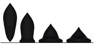
In contrast with Newtonian impacting drops (Yarin Reference Yarin2006; Josserand & Thoroddsen Reference Josserand and Thoroddsen2016), very few studies have been reported on the impact of viscoplastic drops (German & Bertola Reference German and Bertola2009; Luu & Forterre Reference Luu and Forterre2009; Kim & Baek Reference Kim and Baek2012; Luu & Forterre Reference Luu and Forterre2014; Blackwell et al. Reference Blackwell, Deetjen, Gaudio and Ewoldt2015; Oishi, Thompson & Martins Reference Oishi, Thompson and Martins2019; Jørgensen, Forterre & Lhuissier Reference Jørgensen, Forterre and Lhuissier2020; Sen, Morales & Ewoldt Reference Sen, Morales and Ewoldt2020), which emerges from their complex nature. Some of the differences between Newtonian and viscoplastic impact scenarios are illustrated in figure 1, where experimental snapshots show the spreading evolution of a water drop (figure 1a), as well as bentonite-in-water drops at three particle mass fractions  $\phi$: 0.5 (figure 1b), 0.55 (figure 1c) and 0.6 (figure 1d). The drops fall freely from a 5 mm diameter nozzle, hitting a hydrophilic acrylic plate (Quetzeri-Santiago et al. Reference Quetzeri-Santiago, Yokoi, Castrejon-Pita and Castrejon-Pita2019) at an impact velocity $U_0$ of $1.25\ {\rm m}\ {\rm s}^{-1}$. As $\phi$ increases, $5\ \mathrm {\mu }{\rm m}$ mineral particles aggregate in house-of-cards-like clusters mainly through electrostatic and Van der Waals interactions (Chafe & Bruyn Reference Chafe and Bruyn2005), building a microstructure that leads ultimately to the appearance of an increasing macroscopic yield stress of 5 Pa, 50 Pa and 500 Pa, respectively. As $\tau _0$ increases, the material resistance to surface-tension-induced deformations during the free fall becomes more pronounced. Consequently, its initial shape moves from spherical/quasi-spherical (figure 1a,b) to prolate-like (figure 1c,d) characterised not only by an initial diameter $D_0$ of 5 mm imposed by the nozzle, but also by an initial height $H_0$ of 12.5 mm. During the spreading process, the impacting kinetic energy is partially converted into surface energy, and partially dissipated by viscoplastic effects until the drop reaches its maximum spreading $D_{max}$ and minimum height $H_{min}$ at the instant $t_{max}$. Kelvin–Helmholtz instabilities induced by liquid–air interactions (Liu et al. Reference Liu, Lo, Li, Liu, Zhao and Xu2021) at low $\phi$ tend to be suppressed by dissipative effects at larger $\tau _0$, while $D_{max}$ decreases. At $\tau _0 = 500$ Pa, the drop exhibits the lowest final spreading level and preserves its top portion, i.e. its bottom part spreads like a viscous liquid, while its upper portion tends to behave like a solid. In these connections, an open issue arises: can one predict $D_{max}$, $H_{min}$ and $t_{max}$ for viscoplastic non-spherical impacting drops? This question is addressed in the present work.

Figure 1. Experimental snapshots showing the spreading evolution of a water drop (a) and bentonite-in-water drops at three particle mass fractions  $\phi$ (b–d). The yield stress $\tau _0$ increases with $\phi$: (a) $\phi =0$, $\tau _0 = 0$ Pa; (b) $\phi =0.5$, $\tau _0 = 5$ Pa; (c) $\phi =0.55$, $\tau _0 = 50$ Pa; and (d) $\phi =0.6$, $\tau _0 = 500$ Pa. The impact velocity is $U_0 = 1.25\ {\rm m}\ {\rm s}^{-1}$. The diameter of the drops is $D_0 = 5$ mm, and the height of the prolate ones is $H_0 = 12.5$ mm. The interval $\Delta t$ between two images is 1.9 ms.
The very few studies on impacting viscoplastic drops conducted up to now (Luu & Forterre Reference Luu and Forterre2009; Oishi et al. Reference Oishi, Thompson and Martins2019) specify that, under negligible surface tension effects, the maximum relative spreading  $D_{max}/D_0$ depends on two dimensionless parameters: the diameter- $m$-based Reynolds number defined for a Herschel–Bulkley fluid as ${{Re}_{m,D} = {\rho U_0^2}/{k (U_0/D_0)^m}}$ (the ratio of the kinetic to the viscous stress) and the plastic number defined as ${Pl} = {\tau _0}/{\rho U_0^2}$ (the ratio of the yield stress to the kinetic stress). More precisely, according to those studies, each ${{Re}_{m,D}}-{Pl}$ couple induces a unique $D_{max}/D_0$ regardless of the volume of the impacting object. This idea is experimentally explored in figure 2, where snapshots illustrate the spreading of three bentonite-in-water drops impacting a hydrophilic acrylic plate at ${{Re}_{m,D}} = 47$ and ${Pl} = 0.18$. In agreement with the reported theoretical arguments, both the top-line and middle-line drops exhibit similar spreading evolutions with a maximum relative spreading $D_{max}/D_0$ of 1.24, although their volumes differ. However, when increasing the volume of the middle-line drop through a simple height enhancement (see figure 2(c) for which $H_0/D_0 = 4$), one observes a distinct spreading dynamics with $D_{max}/D_0 = 1.91$. Such differences indicate that $H_0/D_0$ also plays a relevant role in the spreading dynamics, an effect not considered by the current theory (Luu & Forterre Reference Luu and Forterre2009). Note that aspect ratio effects are also observed when defining the Reynolds number based on the initial height of the drop, ${{Re}_{m,H} = {\rho U_0^2}/{k (U_0/H_0)^m}}$ (height- $m$-based Reynolds number), a result shown by figure 3, where mayonnaise drops with distinct $H_0/D_0$ impacting an acrylic plate at the same ${{Re}_{m,H}}-{Pl}$ exhibit different $D_{max}/D_0$.

Figure 2. Experimental snapshots illustrating the spreading time evolution of three bentonite-in-water drops impacting a hydrophilic acrylic plate at  ${{Re}_{m,D}} = 47$ and ${Pl} = 0.18$. The dimensionless interval $\Delta t^{\ast } = t/t_{max}$ between two images is 0.1428 ( $t_{max}$ being the instant at which the drop achieves its maximum spreading $D_{max}$). Clearly, regardless of the volume of the drop $V_{total}$, $D_{max}/D_0$ is an increasing function of $H_0/D_0$: (a) $V_{total} = 1.64 \times 10^{-8}\ {\rm m}^3$, $H_0/D_0 = 1$, $D_{max}/D_0 = 1.24$; (b) $V_{total} = 6.54 \times 10^{-8}\ {\rm m}^3$, $H_0/D_0 = 1$, $D_{max}/D_0 = 1.24$; (c) $V_{total} = 2.62 \times 10^{-7}\ {\rm m}^3$, $H_0/D_0 = 4$, $D_{max}/D_0 = 1.91$.

Figure 3. Experimental snapshots showing the spreading evolution of two prolate mayonnaise drops impacting an acrylic plate at  ${{Re}_{m,H}} = 18.6$ and ${Pl} = 0.126$. The dimensionless interval $\Delta t^{\ast } = t/t_{max}$ between two images is 0.3334 for the upper-line case, and 0.1667 ms for the bottom-line case. As observed, different initial aspect ratios induce distinct maximum relative spreading: (a) $H_0/D_0 = 3$, $D_{max}/D_0 = 2$; (b) $H_0/D_0 = 8$, ${D_{max}/D_0 = 2.6}$.
In this work, we highlight the fundamental role of viscoplastic drop shape in normal impact. More specifically, we extend the seminal work of Luu & Forterre (Reference Luu and Forterre2009) by analysing the drop initial aspect ratio effect on the spreading dynamics, maximum spreading, minimum height and spreading time of viscoplastic non-spherical drops impacting a solid hydrophilic surface. Our study is conducted through a mixed approach combining three-dimensional (3-D) numerical simulations and experiments. Numerical simulations based on an adaptive variational multi-scale method for two materials (viscoplastic drop and air) are performed and compared with experiments. The latter are either taken from existing literature or carried out with various yield-stress materials, such as Carbopol-based microgels, alginate suspensions, bentonite and kaolin colloidal suspensions, mayonnaise and ketchup. The results are explored in light of energy budget analyses and scaling laws, which stress the investigated problem's physical mechanisms. Lastly, they are summarised in a two-dimensional diagram linking the maximum diameter, minimum height and final shape of the drops with different flow spreading regimes through a single dimensionless parameter called here the impact number, the latter being a function of  ${{Re}_{m,D}}$, ${Pl}$ and $H_0/D_0$.
The organization of the paper is as follows. A detailed description of the physical formulation and the mixed experimental–numerical method is presented in § 2. Experimental/numerical results are discussed in § 3. Finally, conclusions and perspectives are drawn in the closing section.
2. Problem statement: experimental and numerical viscoplastic non-spherical drop impact on a solid
As illustrated in figures 1, 2 and 3, we consider both experimentally and numerically the normal impact of viscoplastic Herschel–Bulkley falling drops of initial diameter  $D_0$, initial height $H_0$, density $\rho$, consistency $k$, flow index $m$ and yield stress $\tau _0$ against a hydrophilic plate. The drop hits the plate at the instant $t_0$ exhibiting an impact velocity $U_0$. It then spreads radially, undergoing shear and wetting the solid surface before achieving a maximum diameter $D_{max}$ and a minimum height $H_{min}$ at the instant $t_{max}$. The eventual retraction of the drop induced by surface tension effects is not considered here. Splashing events are not taken into account either (Peters, Xu & Jaeger Reference Peters, Xu and Jaeger2013; Blackwell et al. Reference Blackwell, Deetjen, Gaudio and Ewoldt2015; Josserand & Thoroddsen Reference Josserand and Thoroddsen2016). The drop and the plate are surrounded by air whose density is $\rho _{air}$ and viscosity is $\eta _{air}$. Surface tension between the different phases of the system is denoted by $\sigma$.
The drop behaviour is described only through gravitational, inertial, capillary and viscoplastic Herschel–Bulkley parameters. Nevertheless, we show that such physical ingredients are sufficient to capture the main features observed in our experiments.
The important dimensionless quantities of the problem  $\varPi _i$ can be stressed by a classical dimensional analysis based on the Buckingham- $\varPi$ theorem with the following dimensional variables $H_0$, $D_0$, $U_0$, $g$,
$g$,  $\rho$, $k$,
$k$,  $m$,
$m$,  $\tau _0$ and $\sigma$. By doing so, one finds that
 \begin{align} \varPi_1 = \frac{H_0}{D_0},\quad \varPi_2 = \frac{k \left(U_0/D_0 \right)^m}{\rho U_0^2}, \quad \varPi_3 = \frac{\tau_0}{\rho U_0^2}, \quad \varPi_4 = \frac{\rho g D_0}{\rho U_0^2}, \quad \mathrm{and} \quad \varPi_5 = \frac{\sigma/D_0}{\rho U_0^2} , \end{align}
where  $\varPi _2 = 1/{{Re}_{m,D}}$, $\varPi _3 = {Pl}$, $\varPi _4 = 1/{Fr}$ (in which ${Fr}$ is the Froude number) and ${\varPi _5 = 1/{We}}$ (where ${We}$ is the Weber number). Since we consider here centimetric/millimetric drops for which $k$ and/or $\tau _0$ are/is relatively high, $\rho g D_0$ and $\sigma /D_0$ end up playing a marginal role in comparison to the other stress terms, i.e. $\varPi _4 \leq 0.1$ and $\varPi _5 \leq 0.01$ (this will be shown in detail in the following subsection). This particular problem can be explored with the first three dimensionless parameters listed above: $H_0/D_0$, ${{Re}_{m,D}}$ and ${Pl}$.
Alternatively, the important dimensionless quantities of the problem can be stressed by assuming that both the impacting gravitational potential energy of the drop ( ${\sim }\rho g H_0 (H_0 D_0^2)$), and its kinetic energy ( ${\sim }\rho U_0^2 (H_0 D_0^2)$) are partially dissipated by viscoplastic effects (estimated at first glance as ${\sim }k(U_0/H_0)^m D_0^3 + \tau _0 D_0^3$), as well as partially converted into surface energy (approximated as ${\sim }(\sigma /D_0) (H_0 D_0^2)$ at this stage of the present work) during the spreading process
 \begin{equation} \rho g H_0 \Big( H_0 D_0^2 \Big) + \rho U_0^2 \Big( H_0 D_0^2 \Big) \sim k \left( \frac{U_0}{H_0} \right)^m D_0^3 + \tau_0 D_0^3 + \frac{\sigma}{D_0} \Big( H_0 D_0^2 \Big) \end{equation}
(a better estimation of the right-hand side terms will be given in § 3). As underlined earlier, centimetric/millimetric drops for which  $k$ and/or $\tau _0$ are/is relatively high (such as those used here) lead to marginal $\rho g H_0 (H_0 D_0^2)$ and $\rho g H_0 (H_0 D_0^2)$ in comparison to the other energy terms. Furthermore, in the present work ${(k (U_0/H_0)^m + \tau _0) }/{(\sigma /D_0)} > 10$ (a point detailed in the following subsection). Thus, the above equation is rewritten as
 \begin{equation} \rho U_0^2 \sim k \left( \frac{U_0}{D_0} \right)^m \left( \frac{D_0}{H_0} \right)^{m+1} + \tau_0 \left( \frac{D_0}{H_0} \right) , \end{equation}
underlining that the impacting kinetic energy of the drop is mainly dissipated by both viscous and plastic effects during spreading. As a result, at least two spreading scenarios are expected to occur: inertio-viscous (balancing kinetic and viscous stresses) and inertio-plastic (balancing kinetic and yield stresses). By dividing the above equation by  $\rho U_0^2$ (driving stress), one finds that
 \begin{equation} 1 \sim \frac{1}{Re} \frac{D_0}{H_0} , \end{equation}
in which  ${Re}$ is the Reynolds number (similar to Blackwell et al. Reference Blackwell, Deetjen, Gaudio and Ewoldt2015; Thompson, Sica & de Souza Mendes Reference Thompson, Sica and de Souza Mendes2018; Sen et al. Reference Sen, Morales and Ewoldt2020). Clearly, (2.4) indicates that the drop spreading considered here is essentially a dissipative process exposed to shape effects. Finally, aiming to make our study directly comparable to the one conducted by Luu & Forterre (Reference Luu and Forterre2009), the right-hand side term of the above equation is divided into
 \begin{equation} 1 \sim \frac{1}{ {{Re}_{m,D}} } \left( \frac{D_0}{H_0} \right)^{m+1} + {Pl} \left( \frac{D_0}{H_0} \right) , \end{equation}
which underlines that the relevant dimensionless parameters of the problem are  ${{Re}_{m,D}}$, ${Pl}$ and $H_0/D_0$, as previously pointed out by Buckingham- $\varPi$-theorem-based analyses. Their effects on the spreading process will be highlighted in § 3.
2.1. Experimental approach
The experimental set-up for the investigation of the role of viscoplastic drop shape during impact is illustrated in figure 4. The viscoplastic drop of height  $H_0$ and diameter $D_0$ falls by gravity $\boldsymbol {g}$ from a nozzle and hits the solid acrylic plate at the instant $t_0$ at an impact velocity $U_0$. The drop aspect ratio is imposed by controlling the fluid volume within the nozzle, while $U_0$ is a function of the distance between the nozzle and the plate $H$ (
$H$ ( $U_0 \propto \sqrt {H}$). Impact events are experimentally recorded by a Optronis Cyclone 2-2000 high-speed camera ( $ O ( 10^{4} )$ frames per second) equipped with a Sigma 105 mm F2.8 DG OS HSM macro lens, and with the aid of a LED backlight panel. Initial drop diameters $D_0$ are in the range of 2–20 mm, while the initial drop heights $H_0$ vary from 2 mm to 40 mm, and the impact velocities $U_0$ vary from $1\ {\rm m}\ {\rm s}^{-1}$ to $4\ {\rm m}\ {\rm s}^{-1}$. The hydrophilic plate is acrylic (Quetzeri-Santiago et al. Reference Quetzeri-Santiago, Yokoi, Castrejon-Pita and Castrejon-Pita2019). A variety of fluids are used: sodium alginate in 40 % by weight zirconia-in-deionized-water solutions (A); Carbopol-based microgels (C); $5\ \mathrm {\mu }{\rm m}$ bentonite particles in deionized water (B-W); $5\ \mathrm {\mu }{\rm m}$ bentonite particles in 50 % by weight glycerol-in-deionized-water solution (B-G-W); $5\ \mathrm {\mu }{\rm m}$ kaolin particles in deionized water (K-W); Amora, Bénédicta and Hellmann's mayonnaises (M); and Amora, Nature and Heinz ketchups (K). Suspensions at different concentrations are prepared by following the procedures detailed in Luu & Forterre (Reference Luu and Forterre2009) and Godefroid (Reference Godefroid2019).

Figure 4. (a) Experimental set-up for the investigation of the role of viscoplastic drop shape in impact. The viscoplastic drop of height  $H_0$ and diameter $D_0$ falls by gravity $\boldsymbol {g}$ from a nozzle and hits the solid acrylic plate at the instant $t_0$ at an impact velocity $U_0$ ( $U_0$ being a function of the distance between the nozzle and the plate $H$;
$H$;  $U_0 \propto \sqrt {H}$). (b) After the impact, the drop spreads radially until it achieves a maximum diameter $D_{max}$ and a minimum height $H_{min}$ at the instant $t_{max}$. A ketchup drop is used for the illustrated impact event ( $U_0 = 1.25\ {\rm m}\ {\rm s}^{-1}$, $D_0 = 5$ mm, $H_0 = 7.5$ mm, $\rho = 1250\ {\rm kg}\ {\rm m}^{-3}$, $k = 10\ {\rm Pa}\ {\rm s}^{m}$, $m = 0.5$, $\tau _0 = 12$ Pa and $D_{max}/D_0 = 1.82$). It is recorded by a high-speed camera ( $ O ( 10^{4} )$ frames per second) with the aid of a LED backlight panel. A movie showing the mentioned impact event is available as a supplemental material at https://doi.org/10.1017/jfm.2023.926 (see supplementary movie 1).
Although the fluids listed above present a viscoplastic behaviour, they are of different natures and microstructures. This diversity allows for a variety of accessible yield stresses and flow behaviours (from viscoplastic to almost purely plastic suspensions). Mayonnaise (though in reality more complex than that) can be seen as an oil-in-water emulsion with micrometric-sized droplets (Ma & Barbosa-Cánovas Reference Ma and Barbosa-Cánovas1995a,Reference Ma and Barbosa-Cánovasb; Derkach Reference Derkach2009). Ketchup is a tomato paste that can be seen as a organic suspension (Bottiglieri et al. Reference Bottiglieri, de Sio, Fasanaro, Mojoli, Impembo and Castaldo1991; Coussot & Gaulard Reference Coussot and Gaulard2005; Koocheki et al. Reference Koocheki, Ghandi, Razavi, Mortazavi and Vasiljevic2009). Bentonite and kaolin in deionized water and in a glycerol-in-deionized-water solution, in turn, are clay suspensions made of micrometric sheet-like particles that interact between them thanks to van der Waals and electrostatic forces (Luu & Forterre Reference Luu and Forterre2009; Loisel et al. Reference Loisel, Abbas, Masbernat and Climent2015; Mwasame, Wagner & Beris Reference Mwasame, Wagner and Beris2016; Vázquez-Quesada & Ellero Reference Vázquez-Quesada and Ellero2016; Chun et al. Reference Chun, Kwon, Jung and Hyun2017; Tanner Reference Tanner2018; Lin et al. Reference Lin, Zhu, Wang, Chen, Phan-Thien and Pan2019). They can form house-of-cards structures, since the electric charges of the edges and the centres of the particles are different (in both water and glycerol-in-water solution). Arrangements can become more complex, depending on ion concentration in solution and pH (forming aggregates, pillars or more homogeneous structures). Yield stress emerges from the network percolation and is also dependent on solid concentration. In addition, Carbopol microgels are crosslinked acrylic acid polymers that swell in water (Coussot Reference Coussot2007; Paiu Reference Paiu2007; Balmforth et al. Reference Balmforth, Frigaard and Ovarlez2014). Finally, the alginate suspensions are composed of a charged biopolymer (alginate) and zirconia particles, which gives rise to a yield-stress fluid due to depletion interactions (Godefroid Reference Godefroid2019).
Solid content, pH and ion concentration play an important role in the rheological parameters of the used fluids. Although we do not plan to discuss relationships between rheology and microstructure in the present work, it is worth mentioning that we do characterise the fresh materials just before the impact experiments to ensure the use of accurate rheological parameter values.
The used fluids are rheologically characterised using an ARES-G2 rheometer (TA Instruments) equipped with a cone-plate geometry. Their relevant properties and concentrations are listed in table 1. Experimental data available in the literature are also considered. As indicated by the yield stress and the storage modulus  $G^{\prime }$ levels, these materials exhibit elasto-viscoplastic characteristics. Some of them are illustrated in figure 5 where the shear stress is displayed as a function of $| \boldsymbol {\dot {\gamma }} |$ (figure 5a), and $G^{\prime }$ is plotted as a function of the shear stress (figure 5b) for four samples: 57 % by weight bentonite-in-deionized-water (colloidal suspension; grey circles); 3 % by weight Carbopol microgel (polymers; blue triangles); Nature ketchup (organic suspension; red diamonds); and Amora mayonnaise (emulsion; green squares). However, except for the alginate drops, elasticity does not play a relevant role in the impact events studied here, which is underlined by comparing the estimated relaxation time $\lambda$ of the considered materials ( $\lambda \approx ( k/G^{\prime } )^{1/m}$; Luu & Forterre Reference Luu and Forterre2009) to the flow characteristic time $H_0/U_0$, i.e. ${De} = {( k/G^{\prime } )^{1/m}}/{ ( H_0/U_0 ) } < 1$, where ${De}$ is the Deborah number (we set specific values of $H_0$, $D_0$ and $U_0$ allowing ${De}$ to keep lower than 1). Nevertheless, the alginate suspensions used here can be slightly exposed to elastic effects since, for these drops, $1.68 \leq {De} \leq 6.7$. Moreover, although some of the used fluids can be affected by further non-Newtonian signatures, such as microstructural orientation/anisotropy and thixotropy (their mechanical properties can evolve at rest; see the Appendix for a brief discussion on thixotropy; Pignon, Magnin & Piau Reference Pignon, Magnin and Piau1996; Coussot Reference Coussot2005; Coussot et al. Reference Coussot, Roussel, Jarny and Chanson2005; Paiu Reference Paiu2007; Balmforth, Forterre & Pouliquen Reference Balmforth, Forterre and Pouliquen2009; Balmforth et al. Reference Balmforth, Frigaard and Ovarlez2014), none of these are taken into account given the size of our drops (millimetric/centimetric), the axisymmetric nature of the problem and its typical impact/spreading time scale (few ms; similar to Luu & Forterre Reference Luu and Forterre2009, Reference Luu and Forterre2014). Lastly, since most surface tension measurement methods are corrupted by the fluid yield stress and elasticity, we follow previous works (Luu & Forterre Reference Luu and Forterre2009; Jalaal et al. Reference Jalaal, Kemper and Lohse2019) and take pure water surface tension as an upper bound for the real $\sigma$ of our fluids, i.e. $\sigma < 0.072\ {\rm N}\ {\rm m}^{-1}$. As a result, one can show that, for the flow cases analysed here, the ratio of the viscoplastic stress to the capillary stress is always greater than 10, i.e. ${Ca} = ({k (U_0/H_0)^m + \tau _0 })/{(\sigma /D_0)} > 10$, where ${Ca}$ is the capillary number (except for alginate whose ${Ca}$ is around 1). In other words, surface tension plays a marginal role (which will be shown in detail in § 3) when compared with viscoplastic effects. In these connections, we have also neglected any wetting phenomenon (such as hysteresis and dissipation at the contact line) that may particularly affect the receding dynamics (Richard, Clanet & Quéré Reference Richard, Clanet and Quéré2002; de Gennes, Brochard-Wyart & Quéré Reference de Gennes, Brochard-Wyart and Quéré2005; Nigen Reference Nigen2005; Quéré Reference Quéré2008; Bonn et al. Reference Bonn, Eggers, Indekeu, Meunier and Rolley2009; Duez et al. Reference Duez, Ybert, Clanet and Bocquet2010; Carlson, Do-Quang & Amberg Reference Carlson, Do-Quang and Amberg2011).
Table 1. Details concerning the considered fluids for the experiments:  ${\rm A} = \text {sodium}$ alginate in 40 % by weight zirconia-in-deionized-water solutions; ${\rm C} = \text {Carbopol}$-based microgels; $\text {B-W} = 5\ \mathrm {\mu }{\rm m}$ bentonite particles in deionized water; $\text {B-G-W} = 5\ \mathrm {\mu }{\rm m}$ bentonite particles in 50 % by weight glycerol-in-deionized-water solution; $\text {K-W} = 5\ \mathrm {\mu }{\rm m}$ kaolin particles in deionized water; ${\rm M} = {\rm Amora}$, Bénédicta and Hellmann's mayonnaises; ${\rm K} = {\rm Amora}$, Nature and Heinz ketchups. Impact velocities $U_0$ vary from $1\ {\rm m}\ {\rm s}^{-1}$ to $4\ {\rm m}\ {\rm s}^{-1}$.


Figure 5. Rheological characterisation using an ARES-G2 rheometer (TA Instruments) equipped with a cone-plate geometry. We employ standard ramp shear tests over a range of  $10^{-3}\ {\rm s}^{-1}$ to $10^3\ {\rm s}^{-1}$ to obtain stress versus deformation rate levels (a) in addition to oscillatory tests at $10\ {\rm rad}\ {\rm s}^{-1}$ to obtain the storage modulus of the used fluids (b).
2.2. Numerical approach
Our multiphase computational approach is based on a general solver (CIMLIB-CFD, a parallel, finite element library; Coupez & Hachem Reference Coupez and Hachem2013) that takes into account the rheological behaviour of each fluid phase (viscoplastic drop and air; figure 6), as well as surface tension effects (Riber et al. Reference Riber, Valette, Mesri and Hachem2016; Pereira et al. Reference Pereira, Larcher, Hachem and Valette2019; Valette et al. Reference Valette, Hachem, Khalloufi, Pereira, Mackley and Butler2019; Pereira, Hachem & Valette Reference Pereira, Hachem and Valette2020; Valette et al. Reference Valette, Pereira, Riber, Sardo, Larcher and Hachem2021). More precisely, the momentum equation applied to the considered solenoidal flows ( $\boldsymbol {\nabla } \boldsymbol {\cdot } \boldsymbol {u} = 0$) reads
 \begin{equation} \rho \left( \frac{\partial \boldsymbol{u}}{\partial t} + \boldsymbol{u} \boldsymbol{\cdot} \boldsymbol{\nabla} \boldsymbol{u} - \boldsymbol{g} \right) ={-} \boldsymbol{\nabla} p + \boldsymbol{\nabla} \boldsymbol{\cdot} \boldsymbol{\tau} + \boldsymbol{f_{st}} , \end{equation}
in which  $\boldsymbol {u}$, $p$,
$p$,  $\boldsymbol {\tau }$, $\boldsymbol {\nabla }$, $\boldsymbol {g}$, $\boldsymbol {\nabla }\boldsymbol {\cdot }$ and $\boldsymbol {f_{st}}$ are, respectively, the velocity vector, the pressure, the extra-stress tensor, the gradient operator, the gravity vector, the divergence operator and a capillary term related to the surface tension force. The latter is defined as $\boldsymbol {f_{st}} = -\sigma \kappa \varPhi \boldsymbol {n}$, where $\sigma$, $\kappa$, $\varPhi$ and $\boldsymbol {n}$ are the surface tension, the curvature of the drop surface, the Dirac function locating the drop surface and its normal vector, respectively. In addition, the extra-stress tensor is given by $\boldsymbol {\tau } = \eta \boldsymbol {\dot {\gamma }}$, in which $\boldsymbol {\dot {\gamma }}$ represents the rate-of-strain tensor defined as $\boldsymbol {\dot {\gamma }} = ( \boldsymbol {\nabla } \boldsymbol {u} + \boldsymbol {\nabla } \boldsymbol {u}^T)$. The norm of $\boldsymbol {\dot {\gamma }}$ is called the deformation rate, being defined as $| \boldsymbol {\dot {\gamma }} | = ( \frac {1}{2} \boldsymbol {\dot {\gamma }}: \boldsymbol {\dot {\gamma }} ) ^{{1}/{2}}$. The complex drop viscosity $\eta$ is computed using a Herschel–Bulkley equation (Herschel & Bulkley Reference Herschel and Bulkley1926) combined with a Papanastasiou regularization (exponential parts in the following equation; Papanastasiou Reference Papanastasiou1987)
 \begin{equation} \eta
= k {\mid \boldsymbol{{\dot{\gamma}}} \mid}^{m-1} (
{1-{\rm e}^{{\mid -\boldsymbol{{\dot{\gamma}}}
\mid}/{\dot{\gamma_p}}}} )^{1-m} +
\frac{\tau_0}{{\mid \boldsymbol{{\dot{\gamma}}}
\mid}}( {1-{\rm e}^{{\mid -\boldsymbol{{\dot{\gamma}}}
\mid}/{\dot{\gamma_p}}}} ) ,
\end{equation}
\begin{equation} \eta
= k {\mid \boldsymbol{{\dot{\gamma}}} \mid}^{m-1} (
{1-{\rm e}^{{\mid -\boldsymbol{{\dot{\gamma}}}
\mid}/{\dot{\gamma_p}}}} )^{1-m} +
\frac{\tau_0}{{\mid \boldsymbol{{\dot{\gamma}}}
\mid}}( {1-{\rm e}^{{\mid -\boldsymbol{{\dot{\gamma}}}
\mid}/{\dot{\gamma_p}}}} ) ,
\end{equation}
where  ${\dot {\gamma _p}}$ is the cutoff deformation rate (fixed at ${\dot {\gamma _p}} = 10^{-6}\ {\rm s}^{-1}$) that allows us to bound the value of the viscosity for vanishing ${\mid \boldsymbol {{\dot {\gamma }}} \mid }$ below ${\dot {\gamma _p}}$.

Figure 6. Four different drop initial shapes are numerically considered: (a) spherical, (b) prolate,(c) cylindrical and (d) prismatic. Their initial aspect ratio  $H_0/D_0$ varies from 1 to 8. (e) Numerical configuration taken into account. The used mesh (composed of approximately $10^6$ elements) adapted around each interface (viscoplastic drop in red, and air in blue) and illustrated by the black lines. The drop of height $H_0$ and diameter $D_0$ falls by gravity and hits the solid plate at the instant $t_0$ at an impact velocity $U_0$. After the impact, the drop spreads until it achieves a maximum diameter $D_{max}$ and a minimum height $H_{min}$ at the instant $t_{max}$. A movie showing a typical numerical simulation is available as a supplemental material (see supplementary movie 2; $U_0 = 1.5\ {\rm m}\ {\rm s}^{-1}$, $D_0 = 3.15$ mm, $H_0 = 12.6$ mm, $\rho = 1585\ {\rm kg}\ {\rm m}^{-3}$, $k = 0.1\ {\rm Pa}\ {\rm s}^m$, $m = 1$, $\tau _0 = 948$ Pa).
Our numerical methods are based on a variational multi-scale approach combined with anisotropic mesh adaptation with highly stretched elements illustrated by the black lines in figure 6(e) (size of the smaller mesh elements  ${\sim }1\ \mathrm {\mu }{\rm m}$; Riber et al. Reference Riber, Valette, Mesri and Hachem2016; Valette et al. Reference Valette, Hachem, Khalloufi, Pereira, Mackley and Butler2019; Pereira et al. Reference Pereira, Larcher, Hachem and Valette2019, Reference Pereira, Hachem and Valette2020; Valette et al. Reference Valette, Pereira, Riber, Sardo, Larcher and Hachem2021). The time evolution of the drop surface is captured using a level-set function (Hachem et al. Reference Hachem, Khalloufi, Bruchon, Valette and Mesri2016).
The 3-D numerical configuration taken into account is illustrated in figure 6(e), where the mesh (composed of approximately  $10^6$ elements) is depicted, adapted around each interface. The corresponding zero isovalues for the level-set function are also shown (in red). Four different drop initial shapes are numerically considered, as displayed in figures 6(a)–6(d): spherical, prolate, cylindrical and prismatic. Their initial aspect ratio $H_0/D_0$ varies from 1 to 8. Furthermore, a wide range of drop rheological properties is explored, as detailed in table 2, while the impact velocity varies from $0.5\ {\rm m}\ {\rm s}^{-1}$ to $10\ {\rm m}\ {\rm s}^{-1}$. Concerning the air phase (blue region in figure 6), both viscosity $\eta _{air}$ and density $\rho _{air}$ are constant and respectively equal to $10^{-5}\ {\rm Pa}\ {\rm s}$ and $1\ {\rm kg}\ {\rm m}^{-3}$. Lastly, initial and boundary conditions for the flow equations are, respectively, initial vertical impact velocity $U_0$ within the drop, no-slip condition between the fluids and the impacted surface (bottom plate), and zero normal stress in the other walls of the domain.
Table 2. Details concerning the considered drops for the numerical simulations. Impact velocities  $U_0$ vary from $0.5\ {\rm m}\ {\rm s}^{-1}$ to $10\ {\rm m}\ {\rm s}^{-1}$.

3. Results and discussions
3.1. Spreading dynamics
Following the analyses stressed in figure 2, supplemental aspect ratio effects are given by 3-D numerical results in figure 7. The latter shows six numerical snapshots of the spreading process for eight viscoplastic drops at two  ${{Re}_{m,D}}-{Pl}$ couples: ${{Re}_{m,D}} = 50$ and ${Pl} = 0.6$ (figure 7a–d; left column); and ${{Re}_{m,D}} = 150$ and ${Pl} = 0.07$ (figure 7e–h; right column). The interval $\Delta t$ between two subsequent images correspond to 20 % of the necessary time to achieve the maximum spreading $t_{max}$ ( $\Delta t^{\ast } = \Delta t / t_{max} = 0.2$). The red surface in both the first and the last snapshot denotes the 3-D drop–air interface. Contours of the norm of the instantaneous velocity $| u(x, y, z, t) |$ (made dimensionless by the maximum instantaneous velocity $| u_{max}(t) |$) on the centre $x$–
$x$– $z$ plane are represented on the left side of the second through fifth snapshot of each displayed case. Yielded (flowing; $| \boldsymbol {\tau } | > \tau _0$; black) and unyielded (non-flowing; $| \boldsymbol {\tau } | \leq \tau _0$; grey) regions are illustrated on their right side. During the spreading process, the drops develop shear flow within the yielded regions as a result of the no-slip interactions between the solid surface and the viscoplastic material. The more ${{Re}_{m,D}}$ increases and ${Pl}$ decreases (moving from the left-column results to the right-column ones), the more the drops behave like a liquid and spread. Note also that for a fixed ${{Re}_{m,D}}-{Pl}$, (i) viscoplastic drops with different volumes but equal aspect ratios exhibit the same spreading dynamics (velocity field, yielded/unyielded regions and maximum relative spreading); and (ii) viscoplastic drops with distinct aspect ratios present contrasting spreading dynamics even when they exhibit the same volume, as observed by comparing figure 7(b) to figure 7(d), and/or figure 7( f) to figure 7(h). Additionally, the volume of unyielded regions is accentuated by the increase of $H_0/D_0$. More specifically, high aspect ratio drops tend to preserve their upper portion (solid-like portion), while their bottom part spreads like a liquid, dissipating the kinetic energy. Such a deformation localisation within the bottom portion of the material naturally leads to $D_{max}/D_0$ levels greater than those observed for smaller aspect ratio objects impacting at the same ${{Re}_{m,D}}-{Pl}$. Hence, $D_{max}/D_0$ appears as an increasing function of $H_0/D_0$. Obviously, once the kinetic energy is completely dissipated ( $| u(x, y, z, t) | = 0\ {\rm m}\ {\rm s}^{-1}$), the whole drop behaves like a solid, as highlighted by the grey region in the last snapshot of each case.

Figure 7. Six numerical snapshots of the spreading process for eight viscoplastic drops at two  ${{Re}_{m,D}}-{Pl}$ couples: ${{Re}_{m,D}} = 50$ and ${Pl} = 0.6$ (figure 7a–d; left column); ${{Re}_{m,D}} = 150$ and ${Pl} = 0.07$ (figure 7e–h; right column). The interval $\Delta t$ between two subsequent images corresponds to 20 % of the necessary time to achieve the maximum spreading $t_{max}$ ( $\Delta t^{\ast } = \Delta t / t_{max} = 0.2$). The drop volumes, their aspect ratio and their maximum relative spreading are respectively: (a) $V_{total} = 1.64 \times 10^{-8}\ {\rm m}^3$, $H_0/D_0 = 1$, $D_{max}/D_0 = 1.12$; (b) $V_{total} = 6.54 \times 10^{-8}\ {\rm m}^3$, $H_0/D_0 = 1$, $D_{max}/D_0 = 1.12$; (c) $V_{total} = 2.62 \times 10^{-7}\ {\rm m}^3$, $H_0/D_0 = 4$, $D_{max}/D_0 = 1.31$; (d) $V_{total} = 6.54 \times 10^{-8}\ {\rm m}^3$, $H_0/D_0 = 4$, $D_{max}/D_0 = 1.31$; (e) $V_{total} = 1.64 \times 10^{-8}\ {\rm m}^3$, $H_0/D_0 = 1$, $D_{max}/D_0 = 1.8$; ( f) $V_{total} = 6.54 \times 10^{-8}\ {\rm m}^3$, $H_0/D_0 = 1$, $D_{max}/D_0 = 1.8$; (g) $V_{total} = 2.62 \times 10^{-7}\ {\rm m}^3$, $H_0/D_0 = 4$, $D_{max}/D_0 = 2.58$; (h) $V_{total} = 6.54 \times 10^{-8}\ {\rm m}^3$, $H_0/D_0 = 4$, $D_{max}/D_0 = 2.58$. The red surface in both the first and the last snapshot indicates the 3-D drop–air interface. Contours of the norm of the instantaneous velocity $| u(x, y, z, t) |$ (made dimensionless by the maximum instantaneous velocity $| u_{max}(t) |$) on the centre $x$–
$x$– $z$ plane are represented on the left side of the second through fifth snapshot of each displayed case. Yielded (flowing; $| \boldsymbol {\tau } | > \tau _0$; black) and unyielded (non-flowing; $| \boldsymbol {\tau } | \leq \tau _0$; grey) regions are illustrated on their right side.
Aspect ratio effects are equally observed when considering the height-based Reynolds number  ${{Re}_{m,H}}$. In figure 8, six numerical snapshots illustrate the time evolution of spherical (figure 8a) and prolate drops (figure 8b,c) impacting at ${{Re}_{m,H}} = 150$ and ${Pl} = 0.07$. As in figure 7, contours of the norm of the instantaneous velocity $| u(x, y, z, t) |$ (made dimensionless by the maximum instantaneous velocity $| u_{max}(t) |$) on the centre $x$–
$x$– $z$ plane are represented on the left side of the second through fifth snapshot of each displayed case. Yielded (flowing; black) and unyielded (non-flowing; grey) regions are displayed on their right side. As observed by comparing figures 8(a) and 8(c), drops sharing the same volume but a distinct aspect ratio exhibit different velocity field, yielded/unyielded regions and maximum relative spreading. However, at a fixed aspect ratio, the drops present the same impact dynamics, regardless of their volume, as seen by examining figures 8(b) and 8(c).

Figure 8. Six numerical snaphots obtained at  ${{Re}_{m,H}} = 150$ and ${Pl} = 0.07$ illustrate the spreading evolution of spherical and prolate drops: (a) $V_{total} = 2.62 \times 10^{-7}\ {\rm m}^3$, $H_0/D_0 = 1$, $D_{max}/D_0 = 1.8$; (b) $V_{total} =1.64\ \times$ $ 10^{-8}\ {\rm m}^3$, $H_0/D_0 = 4$, $D_{max}/D_0 = 2.37$; (c) $V_{total} = 2.62 \times 10^{-7}\ {\rm m}^3$, $H_0/D_0 = 4$, $D_{max}/D_0 = 2.37$. The red surface in both the first and the last snapshot indicates the 3-D drop–air interface. Contours of the norm of the instantaneous velocity $| u(x, y, z, t) |$ (made dimensionless by the maximum instantaneous velocity $| u_{max}(t) |$) on the centre $x$–
$x$– $z$ plane are represented on the left side of the second through fifth snapshot of each displayed case. Yielded (flowing; black) and unyielded (non-flowing; grey) regions are illustrated on their right side.
Further aspect ratio effects are underlined by figure 9, in which the instantaneous volume fraction of unyielded regions  $V_{unyielded}/V_{total}\times 100[\%]$ is plotted as a function of $t/t_{max}$ for spherical (open symbols) and prolate numerical objects ( $H_0/D_0 = 4$; solid symbols). Subfigures are related to ${{Re}_{m,D}}-{Pl}$ couples: ${{Re}_{m,D}} = 50$ and ${Pl} = 0.6$ (figure 9a); ${{Re}_{m,D}} = 150$ and ${Pl} = 0.07$ (figure 9b); ${{Re}_{m,H}} = 150$ and ${Pl} = 0.07$ (figure 9c). Additionally, each symbol form (circle, triangle and diamond) indicates a specific drop volume $V_{total}$. Inset plots stressing the minimum $V_{unyielded}/V_{total}$ are also provided. At a fixed ${{Re}_{m,D}}-{Pl}$, drops with a similar aspect ratio exhibit equal $V_{unyielded}/V_{total}$ curves, regardless of their volume. Moreover, in each subfigure $V_{unyielded}/V_{total}$ appears as an increasing function of $H_0/D_0$. Such a result emerges from the fact that the augmentation of $H_0/D_0$ leads to a deformation localisation within the bottom part of the drop, while its upper part tends to remain unyielded. In the opposite sense, the increase of ${{Re}_{m,D}}$ and the decrease of ${Pl}$ favour the fluidization of the drop, as observed by examining figures 9(a) and 9(b). Hence, the drops tend to behave like a liquid when their impacting inertial stress increases with respect of the viscoplastic one.

Figure 9. Instantaneous volume fraction of unyielded regions  $V_{unyielded}/V_{total}\times 100[\%]$ plotted as a function of dimensionless time $t/t_{max}$ for spherical (open symbols) and prolate numerical objects ( $H_0/D_0 = 4$; solid symbols). For each subfigure, both the Reynolds number and the plastic number are kept fixed: (a) ${{Re}_{m,D}} = 50$ and ${Pl} = 0.6$, (b) ${{Re}_{m,D}} = 150$ and ${Pl} = 0.07$, and (c) ${{Re}_{m,H}} = 150$ and ${Pl} = 0.07$. Each symbol form indicates a specific drop volume $V_{total}$: $V_{total} = 1.64 \times 10^{-8}\ {\rm m}^3$ (circles); $V_{total} = 6.54 \times 10^{-8}\ {\rm m}^3$ (triangles); $V_{total} = 1.64 \times 10^{-7}\ {\rm m}^3$ (diamonds). Inset plots stressing the minimum $V_{unyielded}/V_{total}$ are also provided.
Another interesting aspect ratio effect is shown by figure 10, where the instantaneous relative diameter  $D(t)/D_0$ is plotted as a function of $t/t_{max}$ for spherical (figure 10a) and prolate drops with $H_0/D_0 = 4$ (figure 10b) and $H_0/D_0 = 8$ (figure 10c). Their volume is fixed at $V_{total} = 2.62 \times 10^{-7}\ {\rm m}^3$. In each subfigure, three ${{Re}_{m,D}}-{Pl}$ couples are explored: ${{Re}_{m,D}} = 80$ and ${Pl} = 0.002$ (grey circles); ${{Re}_{m,D}} = 80$ and ${Pl} = 0.03$ (blue triangles); and ${{Re}_{m,D}} = 80$ and ${Pl} = 0.7$ (red diamonds). First, at a constant aspect ratio, the drop spreading is mitigated by the increment of ${Pl}$. Additionally, the enlargement of $H_0/D_0$ leads to higher $D_{max}/D_0$ levels at a fixed ${{Re}_{m,D}}-{Pl}$ couple (compare, for instance, the grey circle curves in figures 10a, 10b and 10c). However, this effect tends to vanish when plasticity increases and, consequently, the drop tends to behave like a solid (note that the red diamond curves are close to one another, while the grey circle curves exhibit very different relative spreading levels). Hence, drops impacting at higher ${Pl}$ are less exposed to aspect ratio effects than those hitting the solid plate at ${Pl}$ close to 0 (fully viscous scenario).

Figure 10. Instantaneous relative diameter  $D(t)/D_0$ as a function of dimensionless time $t/t_{max}$ for spherical (a) and prolate numerical drops at $H_0/D_0 = 4$ (b) and $H_0/D_0 = 8$ (c). Their volume is fixed at $V_{total} = 2.62 \times 10^{-7}\ {\rm m}^3$. In each subfigure, three ${{Re}_{m,D}}-{Pl}$ couples are explored: ${{Re}_{m,D}} = 80$ and ${Pl} = 0.002$ (grey circles), ${{Re}_{m,D}} = 80$ and ${Pl} = 0.03$ (blue triangles), and ${{Re}_{m,D}} = 80$ and ${Pl} = 0.7$ (red diamonds).
3.2. Energy transfer analyses
Aiming to highlight the physical mechanism driving the aspect ratio effects presented above, we carry out energy budget analyses. More specifically, in figure 11, energy percentage curves are plotted as a function of  $t/t_{max}$: kinetic energy (blue triangles), surface energy (grey circles), gravitational energy (green squares) and dissipation (red diamonds). The latter is divided into two parts: viscous dissipation (orange triangles) and plastic dissipation (black asterisks). These terms are defined as $KE = (1/2) \int _{V}\rho {|\boldsymbol {u}|}^2\,{\rm d}V$ (kinetic energy), $SE = \int _{S} \sigma \,{\rm d}S$ (surface energy), $G = \int _{V} \rho g z \,{\rm d}V$ (gravitational energy), $W = \int _{t} \int _{V} k {| \boldsymbol {{\dot {\gamma }}} |}^{m+1} + \tau _0 {| \boldsymbol {{\dot {\gamma }}} |} \,{\rm d}V \,{\rm d}t$ (dissipation), $W_m = \int _{t} \int _{V} k {| \boldsymbol {{\dot {\gamma }}} |}^{m+1} \,{\rm d}V \,{\rm d}t$ (viscous dissipation) and $W_{\tau _0} = \int _{t} \int _{V} \tau _0 {| \boldsymbol {{\dot {\gamma }}} |} \,{\rm d}V\,{\rm d}t$ (plastic dissipation), where $V$ and $S$ denote the drop volume and surface, respectively (similar to Sanjay, Lohse & Jalaal Reference Sanjay, Lohse and Jalaal2021; Valette et al. Reference Valette, Pereira, Riber, Sardo, Larcher and Hachem2021). Each computed energy term is made dimensionless by the total energy of the system ( $= KE(t = t_0) + SE(t = t_0) + G(t = t_0) + W(t = t_0)$) and generically represented by variable $\varepsilon ^{*}$. Aspect ratio effects on the spreading dynamics are stressed using four different numerical drops: $H_0/D_0 = 1$ and $V_{total} = 6.54 \times 10^{-8}\ {\rm m}^3$ (first line); $H_0/D_0 = 1$ and $V_{total} = 2.62 \times 10^{-7}\ {\rm m}^3$ (second line); $H_0/D_0 = 4$ and $V_{total} = 2.62 \times 10^{-7}\ {\rm m}^3$ (third line); and $H_0/D_0 = 4$ and $V_{total} = 6.54 \times 10^{-8} {\rm m}^3$ (fourth line). For each one of them, three ${{Re}_{m,D}}-{Pl}$ couples are considered: ${{Re}_{m,D}} = 112.5$ and ${Pl} = 0.002$ (a,d,g,j); ${{Re}_{m,D}} = 112.5$ and ${Pl} = 0.05$ (b,e,h,k); and ${{Re}_{m,D}} = 112.5$ and ${Pl} = 0.5$ (c, f,i,l).

Figure 11. Energy percentage curves plotted as a function of dimensionless time  $t/t_{max}$: kinetic energy (blue triangles), surface energy (grey circles), gravitational energy (green squares) and dissipation (red diamonds). The latter is divided into two parts: viscous dissipation (orange triangles) and plastic dissipation (black asterisks). The computed terms are made dimensionless by the total energy of the system and generically represented by variable $\varepsilon ^{*}$. Aspect ratio effects on the spreading dynamics are pointed out with the aid of four different numerical drops: $H_0/D_0 = 1$ and $V_{total} = 6.54 \times 10^{-8}\ {\rm m}^3$ (first line); $H_0/D_0 = 1$ and $V_{total} = 2.62 \times 10^{-7}\ {\rm m}^3$ (second line); $H_0/D_0 = 4$ and $V_{total} = 2.62 \times 10^{-7}\ {\rm m}^3$ (third line); and $H_0/D_0 = 4$ and $V_{total} = 6.54 \times 10^{-8} {\rm m}^3$ (fourth line). For each of them, three ${{Re}_{m,D}}-{Pl}$ couples are considered: ${{Re}_{m,D}} = 112.5$ and ${Pl} = 0.002$ (a,d,g,j); ${{Re}_{m,D}} = 112.5$ and ${Pl} = 0.05$ (b,e,h,k); and ${{Re}_{m,D}} = 112.5$ and ${Pl} = 0.5$ (c, f,i,l).
For all 12 impact events displayed in figure 11, the drop kinetic energy is primarily dissipated during its spreading (note that both the surface energy and the gravitational one play a marginal role in comparison to the other energy terms, as mentioned in § 2). Nevertheless, the dissipative process exhibits particular signatures depending on  ${{Re}_{m,D}}$, ${Pl}$ and $H_0/D_0$. For the drops impacting at ${{Re}_{m,D}} = 112.5$ and ${Pl} = 0.002$, for example, plasticity is negligible and, consequently, dissipation is basically driven by the viscous stress ( $k {| \boldsymbol {{\dot {\gamma }}} |}^{m}$). However, when increasing ${Pl}$ to 0.05 and keeping ${{Re}_{m,D}}$ and $H_0/D_0$ fixed (middle-column results), plastic dissipation becomes comparable to the viscous one ( $\tau _0 {| \boldsymbol {{\dot {\gamma }}} |} \approx k {| \boldsymbol {{\dot {\gamma }}} |}^{m+1}$). Interestingly, the former becomes slightly dominant by increasing $H_0/D_0$ from 1 (spherical) to 4 (prolate), as highlighted by opposing the middle-column results above and below the black horizontal line. Such a result is rather in line with the augmentation of the unyielded volume fraction induced by the increase of aspect ratio exposed in figure 9. It clearly indicates that the shape of the drop affects the dissipative mechanism during the spreading. Logically, plastic effects are strengthened by the increase of ${Pl}$, eventually leading to a plasticity-driven dissipation, as shown by the third-column results. Lastly, it is worth noting that the volume of the drop does not affect the energy percentage curves displayed in figure 11, which can be observed by comparing the top-line curves with the second-line ones (and/or the third-line with the fourth-line curves) at fixed ${{Re}_{m,D}}$ and ${Pl}$.
Supplemental energy transfer analyses are conducted in figures 12 and 13, respectively, for spherical and  $H_0/D_0 = 4$ prolate numerical drops with the same volume $V_{total} = 2.62 \times 10^{-7}\ {\rm m}^3$. Each subfigure is related to a specific ${{Re}_{m,D}}-{Pl}$ couple: ${{Re}_{m,D}} = 112.5$ and ${Pl} = 0.002$ (figures 12a and 13a); ${{Re}_{m,D}} = 112.5$ and ${Pl} = 0.05$ (figures 12b and 13b); and ${{Re}_{m,D}} = 112.5$ and ${Pl} = 0.5$ (figures 12c and 13c). They are composed of six upper-line snapshots and six bottom-line snapshots ( $\Delta t^{\ast } = t/t_{max} = 0.2$). The first one shows the 3-D drop–air interface in red. From the second to the last upper-line snapshot, $| \boldsymbol {{\dot {\gamma }}} |/(U_0/H_0)$ contours are displayed on the left side of the centre $x$–
$x$– $z$ plane, while yielded (black) and unyielded (grey) regions are shown on the right side. Furthermore, from the second to the last bottom-line snapshot, the dissipative process is stressed by $k {|\boldsymbol {{\dot {\gamma }}}|}^{m+1}/(\rho U_0^3/H_0)$ and $\tau _0 {|\boldsymbol {{\dot {\gamma }}}|}/(\rho U_0^3/H_0)$ contours on the left and right side of the centre $x$–
$x$– $z$ plane, respectively. Logically, greater dissipation levels are observed within high deformation rate zones developed at the vicinities of the solid substrate due to the imposed no-slip condition. As ${Pl}$ moves from 0.002 to 0.5, dissipation switches from a viscous-dominated process to a plastic-dominated one, and tends to occur exclusively in the bottom portion of the drop, where the shear stresses overpass $\tau _0$. Such a localisation effect is also favoured by the augmentation of $H_0/D_0$ (figure 13b,c), since shear stresses tend to vanish far from the wall (in the upper portion of the drops) for any impact event. Note, for example, that more than 50 % of the prolate drop shown by the second snapshot in figure 13(a) exhibits a very low deformation rate (blue contour) against less than 25 % for the spherical drop displayed by the corresponding snapshot in figure 12(a). It is equally important to emphasise that the vicinities of the interfaces between yielded (liquid-like) and unyielded (solid-like) zones are characterised by low deformation rate levels, which naturally makes them plasticity-driven from a dissipative standpoint (plastic dissipation is proportional to ${| \boldsymbol {{\dot {\gamma }}} |}$, whereas viscous dissipation is comparable to ${| \boldsymbol {{\dot {\gamma }}} |}^{m+1}$). Hence, the growth of such interfaces induced by the increase of $H_0/D_0$ may lead to a swelling of the plastic dissipation, as observed by comparing spherical to prolate energy curves at a fixed ${{Re}_{m,D}}-{Pl}$ couple in figure 11. Lastly, despite the differences observed at low and high ${Pl}$, it is worth noting that, from an average viewpoint, the height of the dissipative layer remains comparable to $H_{min}$, as pointed out by the magenta dashed line in figures 12(b) and 13(b). For this reason, $H_{min}$ is used to estimate the mean viscous dissipation in the following subsection.

Figure 12. Spherical numerical drops ( $H_0/D_0 = 1$) with the same volume $V_{total} = 2.62 \times 10^{-7}\ {\rm m}^3$. Each subfigure is related to a specific ${{Re}_{m,D}}-{Pl}$ couple: (a) ${{Re}_{m,D}} = 112.5$ and ${Pl} = 0.002$; (b) ${{Re}_{m,D}} = 112.5$ and ${Pl} = 0.05$; (c) ${{Re}_{m,D}} = 112.5$ and ${Pl} = 0.5$. They are composed of six upper-line snapshots and six bottom-line snapshots ( $\Delta t^{\ast } = t/t_{max} = 0.2$). The first one shows the 3-D drop–air interface in red. From the second to the last upper-line snapshot, $| \boldsymbol {{\dot {\gamma }}} |/(U_0/H_0)$ contours are displayed on the left side of the centre $x$–
$x$– $z$ plane, while yielded (black) and unyielded (grey) regions are shown on the right side. Additionally, from the second to the last bottom-line snapshot, the dissipative process is stressed by $k {|\boldsymbol {{\dot {\gamma }}}|}^{m+1}/(\rho U_0^3/H_0)$ and $\tau _0 {|\boldsymbol {{\dot {\gamma }}}|}/(\rho U_0^3/H_0)$ contours on the left and right side of the centre $x$–
$x$– $z$ plane, respectively.

Figure 13. Prolate numerical drops ( $H_0/D_0 = 4$) with the same volume $V_{total} = 2.62 \times 10^{-7}\ {\rm m}^3$. Subfigures are related to specific ${{Re}_{m,D}}-{Pl}$ couples: (a) ${{Re}_{m,D}} = 112.5$ and ${Pl} = 0.002$; (b) ${{Re}_{m,D}} = 112.5$ and ${Pl= 0.05}$; (c) ${{Re}_{m,D}} = 112.5$ and ${Pl} = 0.5$. They are composed of six upper-line snapshots and six bottom-line snapshots ( $\Delta t^{\ast } = t/t_{max} = 0.2$). The first snapshot shows the 3-D drop–air interface in red. From the second to the last upper-line snapshot, $| \boldsymbol {{\dot {\gamma }}} |/(U_0/H_0)$ contours are displayed on the left side of the centre $x$–
$x$– $z$ plane, while yielded (black) and unyielded (grey) regions are shown on the right side. Additionally, from the second to the last bottom-line snapshot, the dissipative process is stressed by $k {|\boldsymbol {{\dot {\gamma }}}|}^{m+1}/(\rho U_0^3/H_0)$ and $\tau _0 {|\boldsymbol {{\dot {\gamma }}}|}/(\rho U_0^3/H_0)$ contours on the left and right side of the centre $x$–
$x$– $z$ plane, respectively.
3.3. Scaling laws: maximum spreading, spreading time, minimum height and final shape
Based on the energy transfer analyses conducted above, we propose scaling laws for  $D_{max}$ by considering at least two spreading regimes: inertio-viscous (figure 11a,d,g,j) and inertio-plastic (figure 11c, f,i,l). The scaling laws are developed in the following paragraph.
In the inertio-viscous spreading regime, the impacting kinetic energy of the drop ( ${\sim }\rho U_0^2 H_0 D_0^2$) is primarily dissipated by viscous effects ( ${\sim }k (U_c/H_{min})^m D_{max}^3$, where $U_c$ represents a characteristic dissipation velocity, which will be approximated, at first glance, as $U_0$). On the other hand, in the inertio-plastic spreading regime, the kinetic energy is mainly dissipated by plastic effects ( ${\sim }\tau _0 D_{max}^3$). Together with mass conservation ( $H_0 D_0^2 \sim H_{min} D_{max}^2$), we conclude that $D_{max}/D_0$ scales as $[ {{Re}_{m,D}} (H_0/D_0)^{m+1} ]^{1/{2m+3}}$ in the former scenario and $[ (1/{Pl})(H_0/D_0) ]^{1/3}$ in the latter. For the inertio-viscous scaling, aspect ratio effects on $D_{max}/D_0$ are amplified by the growth of ${{Re}_{m,D}}$. However, for the inertio-plastic scaling, the drop spreading becomes less exposed to aspect ratio effects as ${Pl}$ increases. Such tendencies are rather in line with the results brought up by figure 10. It is also worth noting that when working with spherical drops ( $H_0/D_0 = 1$) we recover scaling laws previously reported in the literature (Luu & Forterre Reference Luu and Forterre2009), i.e. ${{{Re}_{m,D}}}^{1/{2m+3}}$ (inertio-viscous spreading) and $(1/{Pl})^{1/3}$ (inertio-plastic spreading). Moreover, for Newtonian spherical drops, $m$ is equal to 1, and so $D_{max}/D_0 \sim {{{Re}_{m,D}}}^{1/5}$, as widely cited in the literature (Clanet et al. Reference Clanet, Béguin, Richard and Quéré2004; Laan et al. Reference Laan, de Bruin, Bartolo, Josserand and Bonn2014; Josserand & Thoroddsen Reference Josserand and Thoroddsen2016; Wildeman et al. Reference Wildeman, Visser, Sun and Lohse2016).
By equating the scaling laws presented above, we define the impact number  ${I} = (1/{Pl})^{1/3} (1/{{Re}_{m,D}})^{1/{2m+3}} (H_0/D_0)^{-m/{6m+9}} = 1$, a unifying dimensionless parameter for both the inertio-plastic and the inertio-viscous spreading that approaches to 1 at the transition between the mentioned regimes. In other words, regime transition is expected to occur at ${I} \approx 1$.
The validity of the above theoretical arguments is corroborated by figure 14, in which the rescaled maximum spreading  $(D_{max}/D_0) / [ {{Re}_{m,D}} (H_0/D_0)^{m+1} ]^{1/{2m+3}}$ is plotted as a function of ${I}$ not only for spherical, prolate, cylindrical and prismatic numerical objects but also for spherical and non-spherical experimental drops (asterisks; error bars are comparable to the size of the symbols). More specifically, in figure 14(a) the results are plotted using the impact number definition given by Luu & Forterre (Reference Luu and Forterre2009), $(1/{Pl})^{1/3} (1/{{Re}_{m,D}})^{1/{2m+3}}$, while in figure 14(b) the impact number developed in the present work is used. Comparing these subfigures, we clearly note that, when the aspect ratio effects are taken into account, the points collapse across a single path divided into three regions linked with three spreading regimes: inertio-plastic (I; ${I} \leq 1$; blue box); the inertio-viscous (II; ${I} \geq 3$; red box); and a mixed regime (III; $1 < {I} < 3$; white box), for which inertial, viscous and plastic effects all play an important role (the viscous dissipation is comparable to the plastic one). The mixed inertio-visco-plastic region is defined based on the detachment of the points from both the inertio-plastic scaling (black dash-dotted line) and the inertio-viscous one (black dotted line). Interestingly, for the impact number interval explored here ( $0.2 \leq {I} \leq 100$), the results can be fitted by the following Padé approximant (polynomial expression)
 \begin{equation} {P} = 0.9 \frac{ {I}^3 + {I}^2 + {I} }{ {I}^3 + {I}^2 + {I} + 1} , \end{equation}
which in turn is represented by the red line in figure 14(b). Padé approximants similar to that given in (3.1) are typically employed in drop impact works to represent master curves (Laan et al. Reference Laan, de Bruin, Bartolo, Josserand and Bonn2014; Josserand & Thoroddsen Reference Josserand and Thoroddsen2016). Hence,  $D_{max}/D_0$ can be predicted by the following equation:
 \begin{equation} \frac{D_{max}}{D_0} = {P} \left[ \left( \frac{H_0}{D_0} \right)^{m+1} {{Re}_{m,D}} \right]^{1/{2m+3}} . \end{equation}
Additionally, thanks to the mass conservation ( $\sqrt {H_0/H_{min}} \sim D_{max}/D_0$), we can plot the rescaled minimum height $\sqrt {H_0/H_{min}} / [ {{Re}_{m,D}} (H_0/D_0)^{m+1} ]^{1/{2m+3}}$ as a function of the impact number, as illustrated in figure 14(c). Once again, the points collapse across a single path divided into the three regimes mentioned previously (only numerical results related to prolate drops are shown, for clarity). In inertio-plastic impact events the upper part of the drop tends to preserve its initial shape, while its bottom portion spreads radially. As a result, prolate impacting objects exhibit a more conical shape at the end of the spreading process, as illustrated by the blue drop (see also figures 2c and 13c). However, as plastic effects are attenuated, and consequently ${I}$ increases, the drop final shape becomes flattened (pancake-like, in red), which characterises inertio-viscous impact events (see figures 4b and 13a).

Figure 14. (a) Rescaled maximum spreading plotted using the scaling laws and the impact number definition given by Luu & Forterre (Reference Luu and Forterre2009):  $(D_{max}/D_0) / [ {{Re}_{m,D}} ]^{1/{2m+3}}$ against $(1/{Pl})^{1/3} (1/{{Re}_{m,D}})^{1/{2m+3}}$. (b) Rescaled maximum spreading plotted using the scaling laws and the impact number definition taking the drop aspect ratio into account (present work): $(D_{max}/D_0) / [ {{Re}_{m,D}} (H_0/D_0)^{m+1} ]^{1/{2m+3}}$ against $(1/{Pl})^{1/3} (1/{{Re}_{m,D}})^{1/{2m+3}} (H_0/D_0)^{-m/{6m+9}}$. The symbols denote aspect ratio values (for the numerical simulations) or intervals (for the experiments; asterisks). (c) Rescaled minimum height as a function of the impact number (only numerical results related to prolate drops are plotted, for clarity). (d) Comparisons between the spreading time $t_{max}$ obtained from numerical simulations using prolate drops, and the one predicted by combining (3.4) and (3.2).
It is important to underline that, as observed by examining figure 14(a) with figure 14(b), the augmentation of  $H_0/D_0$ can induce an increase of more than 80 % in $D_{max}/D_0$, in respect to spherical objects. Additionally, although shape effects on the impact number stay relatively low even for the highest aspect ratio drop considered here ( ${<}15\,\%$ for $H_0/D_0 = 8$), they can eventually lead to spreading regime changes, especially for impact events at ${I}$ close to 1 and/or 3 (critical values giving the interfaces between the three impact zones illustrated in figure 14b,c). Hence, the role of drop shape in the impact/spreading process cannot be overestimated.
Lastly, an expression for the drop maximum spreading time is proposed through energy conservation arguments, by considering both the viscous and the plastic source of energy dissipation, i.e.
 \begin{equation} \rho U_0^2 H_0 D_0^2 \sim k (U_c/H_{min})^m D_{max}^3 + \tau_0 D_{max}^3 . \end{equation}
By defining the spreading time  $t_{max} = D_{max}/U_c$, and together with mass conservation ( $H_0 D_0^2 \sim H_{min} D_{max}^2$), we find that
 \begin{equation} t_{max} = \left[ \frac{Ak \left( \dfrac{D_{max}}{D_0} \right)^{3m+3} \left( \dfrac{D_0}{H_0} \right)^{m+1} }{B \rho U_0^2 - C\tau_0 \left( \dfrac{D_0}{H_0} \right) \left( \dfrac{D_{max}}{D_0} \right)^3 } \right]^{1/m} , \end{equation}
where  $A$,
$A$,  $B$ and $C$ are adjustable prefactors, and $D_{max}/D_0$ can be approximated as ${P}[ {{Re}_{m,D}} (H_0/D_0)^{m+1} ]^{1/{2m+3}}$ according to (3.2), ultimately giving us a predicted $t_{max}$. The latter is plotted against the measured $t_{max}$ in figure 14(d) for a wide range of $H_0/D_0$ with $A = 1.25$, $B = 0.4$ and $C = 1$ (for clarity, only numerical results are shown). As observed, both the predicted and the measured spreading time are in good agreement with each other.
In short, figure 14 emphasises that the viscoplastic drop-spreading dynamics is deeply affected by  $H_0/D_0$, which in turn reveals the potential of using drop shape to control spreading.
4. Concluding remarks and perspectives
In this paper we have experimentally and numerically studied the normal impact of viscoplastic drops on a solid plate under negligible capillary effects. We have extended the seminal work reported by Luu & Forterre (Reference Luu and Forterre2009) by highlighting the fundamental role of shape in the normal impact of viscoplastic drops. In this connection, spherical, prolate, cylindrical and prismatic drops have been analysed and their rheological behaviour was expressed through a classical Herschel–Bulkley constitutive equation. Supplemental non-Newtonian signatures such as microstructural orientation/anisotropy and thixotropy have not been considered.
High aspect ratio viscoplastic drops tend to preserve their upper portion (solid-like portion), while their bottom part spreads like a liquid, dissipating the kinetic energy. Such a deformation localisation within the bottom portion of the material naturally leads to  $D_{max}/D_0$ levels greater than those observed for smaller aspect ratio objects impacting at the same ${{Re}_{m,D}}-{Pl}$. Hence, $D_{max}/D_0$ appears as an increasing function of $H_0/D_0$.
In short, results show that the drop impacting kinetic energy is primarily dissipated through viscoplastic effects during the spreading process, giving rise to three flow regimes: (i) inertio-viscous (balancing kinetic and viscous stresses); (ii) inertio-plastic (balancing the kinetic stress and yield stress); and (iii) mixed inertio-visco-plastic (balancing kinetic and viscoplastic stresses). They are highly affected by the initial aspect ratio of the drop, and can be found using the impact number  ${I} = (1/{Pl})^{1/3} (1/{{Re}_{m,D}})^{1/{2m+3}} (H_0/D_0)^{-m/{6m+9}}$. The drop maximum spreading, minimum height, spreading time and final shape are all directly linked with the impact number as well.
Our study has direct applications in a number of impact-based situations, which includes spraying generation, firefighting, inkjet printing, atomization, viscoplastic water entry and 3-D printing of organs, tissues, prosthetics and electronic components, among others (Modak et al. Reference Modak, Kumar, Tripathy and Sen2020; Murphy & Atala Reference Murphy and Atala2020; Vijayavenkataraman et al. Reference Vijayavenkataraman, Yan, Lu, Wang and Fuh2018; Jalaal et al. Reference Jalaal, Kemper and Lohse2019; Lorenceau & Quéré Reference Lorenceau and Quéré2003; Bordoloi & Longmire Reference Bordoloi and Longmire2014; Ryu et al. Reference Ryu, Sen, Nam and Lee2017; Kumar et al. Reference Kumar, Tripathy, Nam, Lee and Sen2018; Soto et al. Reference Soto, Girard, Le Helloco, Binder, Quéré and Varanasi2018; Su et al. Reference Su, Luo, Chu, Cai, Le, Zhang and Chen2020). More specifically, the mentioned applications could benefit from the diagrams highlighted in figure 14, which ultimately could be used to predict and control the spreading dynamics (spreading time, maximum spreading, minimum height and final shapes) of prolate viscoplastic drops impacting on a solid surface (in purely viscoplastic scenarios).
Finally, in terms of perspectives, since complex fluids are highly diffused in industrial domains, it would be interesting to consider in future works supplemental non-Newtonian effects on the spreading dynamics, such as those related to elasticity and/or thixotropy. Similar analyses using bentonite suspensions at lower concentrations ( ${<}50\,\%$ and, consequently, $k \approx 0.01 \ {\rm Pa}\ {\rm s}^m$ and $\tau _0 < 50$ Pa) would be welcome as well since they could be used to explore supplemental spreading regimes balanced by the inertial stress, the capillary pressure and the yield stress.
Supplementary movies
Supplementary movies are available at https://doi.org/10.1017/jfm.2023.926.
Acknowledgements
We would like to thank Mrs C. Borgo for her great help with some of the experiments performed here, as well as Professor C. Ligoure (University of Montpellier) and Dr L. Ramos (University of Montpellier) for fruitful discussions.
Funding
The authors also would like to acknowledge the support from the UCA $^\mathrm {JEDI}$ program (IDEX of Université Côte d'Azur), the PSL Research University under the program ‘Investissements d'Avenir’ launched by the French government and implemented by the French National Research Agency (ANR) with the reference ANR-10-IDEX-0001-02 PSL, and the ANR for supporting the INNpact project under the ‘Jeunes chercheuses et jeunes chercheurs’ program.
Declaration of interests
The authors report no conflict of interest.
Appendix. Thixotropy
Aiming to underline thixotropic effects, we present in figure 15 three-step deformation rate rheological tests for the samples shown in figure 5: 57 % bentonite (figure 15a), 3 % Carbopol (figure 15b), ‘Nature’ ketchup (figure 15c) and ‘Amora’ mayonnaise (figure 15d). These tests were carried out using an ARES-G2 rheometer (TA Instruments) equipped with a cone-plate geometry. At each step, the shear viscosity is plotted as a function of time (over 60 s) at a specific deformation rate:  $0.1\ {\rm s}^{-1}$ at steps 1 and 3; and $100\ {\rm s}^{-1}$ at step 2. An acquisition rate of 10 points per second was chosen. As observed, thixotropic recovery time scales $t_{thixotropy}$ vary from $ O ( 10^0 )$ s (figure 15a–c) to $ O ( 10^1 )$ s (figure 15d), which is at least 100 times longer than the analysed impact events ( $t_{max} \approx O ( 10^{-2} )$ s). Hence, thixotropic effects have not been considered in our theoretical analyses. Nevertheless, since $t_{thixotropy} \gg t_{max}$, future numerical studies focusing on both the local and time evolution of the breakdown/recovery process during the drop spreading would be more than welcome.

Figure 15. Three-step deformation rate rheological tests: 57 % bentonite (a), 3 % Carbopol (b), ‘Nature’ ketchup (c) and ‘Amora’ mayonnaise (d). These tests were carried out using an ARES-G2 rheometer (TA Instruments) equipped with a cone-plate geometry. At each step, the shear viscosity is plotted as a function of time (over 60 s) at a specific deformation rate:  $0.1\ {\rm s}^{-1}$ at steps 1 and 3; and $100\ {\rm s}^{-1}$ at step 2. The black arrows indicate the recovery process.


