


1. Introduction
The secretary problem, also known as the game of Googol, the beauty contest problem, and the dowry problem, was formally introduced in [Reference Gardner8], while the first solution was obtained in [Reference Lindley12]. A widely used version of the secretary problem can be stated as follows: n individuals are ordered without ties according to their qualifications. They apply for a ‘secretary’ position, and are interviewed one by one, in a uniformly random order. When the tth candidate appears, she or he can only be ranked (again without ties) with respect to the $t-1$
already interviewed individuals. At the time of the tth interview, the employer must make the decision to hire the person present or continue with the interview process by rejecting the candidate; rejected candidates cannot be revisited at a later time. The employer succeeds only if the best candidate is hired. If only one selection is to be made, the question of interest is to determine a strategy (i.e. final rule) that maximizes the probability of selecting the best candidate.
$t-1$
already interviewed individuals. At the time of the tth interview, the employer must make the decision to hire the person present or continue with the interview process by rejecting the candidate; rejected candidates cannot be revisited at a later time. The employer succeeds only if the best candidate is hired. If only one selection is to be made, the question of interest is to determine a strategy (i.e. final rule) that maximizes the probability of selecting the best candidate.
In [Reference Lindley12] the problem was solved using algebraic methods with backward recursions, while [Reference Dynkin5] considered the process as a Markov chain. An extension of the secretary problem, known as the dowry problem with multiple choices (for simplicity, we refer to it as the dowry problem), was studied in [Reference Gilbert and Mosteller9]. In the dowry problem, $s>1$
candidates can be selected during the interview process, and the condition for success is that the selected group includes the best candidate. This review process can be motivated in many different ways: for example, the s-selection may represent candidates invited for a second round of interviews. In [Reference Gilbert and Mosteller9] we find a heuristic solution to the dowry problem, while [Reference Sakaguchi19] solved the problem using a functional-equation approach of the dynamic programming method.
$s>1$
candidates can be selected during the interview process, and the condition for success is that the selected group includes the best candidate. This review process can be motivated in many different ways: for example, the s-selection may represent candidates invited for a second round of interviews. In [Reference Gilbert and Mosteller9] we find a heuristic solution to the dowry problem, while [Reference Sakaguchi19] solved the problem using a functional-equation approach of the dynamic programming method.
In [Reference Gilbert and Mosteller9] the authors also offer various extensions to the secretary problem in many different directions. For example, they examine the secretary problem (single choice) when the objective is to maximize the probability of selecting the best or the second-best candidate, while the more generalized version of selecting one of the top $\ell$
candidates was considered in [Reference Gusein-Zade10]. Additionally in [Reference Gilbert and Mosteller9] the authors studied the full information game where the interviewer is allowed to observe the actual values of the candidates, which are chosen independently from a known distribution. Several other extensions have been considered in the literature, including the postdoc problem, for which the objective is to find the second-best candidate [Reference Gilbert and Mosteller9, Reference Rose18], and the problem of selecting all or one of the top
$\ell$
candidates was considered in [Reference Gusein-Zade10]. Additionally in [Reference Gilbert and Mosteller9] the authors studied the full information game where the interviewer is allowed to observe the actual values of the candidates, which are chosen independently from a known distribution. Several other extensions have been considered in the literature, including the postdoc problem, for which the objective is to find the second-best candidate [Reference Gilbert and Mosteller9, Reference Rose18], and the problem of selecting all or one of the top $\ell$
candidates when
$\ell$
candidates when $\ell$
choices are allowed [Reference Nikolaev16, Reference Tamaki21, Reference Tamaki22]. More recently, the problem has been considered under a model where interviews are performed according to a nonuniform distribution such as the Mallows or Ewens [Reference Crews, Jones, Myers, Taalman, Urbanski and Wilson3, Reference Jones11, Reference Liu and Milenkovic13, Reference Liu, Milenkovic and Moustakides14]. For more details regarding the history of the secretary problem, the interested reader may refer to [Reference Ferguson6, Reference Freeman7].
$\ell$
choices are allowed [Reference Nikolaev16, Reference Tamaki21, Reference Tamaki22]. More recently, the problem has been considered under a model where interviews are performed according to a nonuniform distribution such as the Mallows or Ewens [Reference Crews, Jones, Myers, Taalman, Urbanski and Wilson3, Reference Jones11, Reference Liu and Milenkovic13, Reference Liu, Milenkovic and Moustakides14]. For more details regarding the history of the secretary problem, the interested reader may refer to [Reference Ferguson6, Reference Freeman7].
The secretary problem with expert queries, an extension of the secretary problem with multiple choices, was introduced in [Reference Liu, Milenkovic and Moustakides14] and solved using combinatorial methods for a generalized collection of distributions that includes the Mallows distribution. In this extended version it is assumed that the decision-making entity has access to a limited number of infallible experts. When faced with a candidate in the interviewing process an expert, if queried, provides a binary answer of the form ‘the best’ or ‘not the best’. Queries to experts are frequently used in interviews as an additional source of information, and the feedback is usually valuable but is not necessarily accurate. This motivates the investigation of the secretary problem when the response of the expert is not deterministic (infallible) but may also be false. This can be modeled by assuming that the response of the expert is random. Actually, the response does not even have to be binary as in the random query model employed in [Reference Chien, Pan and Milenkovic2, Reference Mazumdar and Saha15] for the completely different problem of clustering. In our analysis we consider more than two possibilities which could reflect the level of confidence of the expert in their knowledge of the current candidate being the best or not. For example a four-level response could be of the form ‘the best with high confidence’, ‘the best with low confidence’, ‘not the best with low confidence’, or ‘not the best with high confidence’. As we will see, the analysis of the problem under a randomized expert model requires stochastic optimization techniques, and in particular results we are going to borrow from optimal stopping theory [Reference Peskir and Shiryaev17, Reference Shiryaev20].
The idea of augmenting the classical information of relative ranks with auxiliary random information (e.g. coming from a fallible expert) has also been addressed in [Reference Dutting, Lattanzi, Leme and Vassilvitskii4]. In this work the authors consider various stochastic models for the auxiliary information, which is assumed to become available to the decision maker with every new candidate. The goal is the same as in the classical secretary problem, namely to optimize the final termination time. This must be compared to the problem we are considering in our current work where auxiliary information becomes available only at querying times, which constitute a sequence of stopping times that must be selected optimally. Furthermore, at each querying time, using the extra information provided by the expert, we also need to decide, optimally, whether we should terminate the selection process at the querying time or continue to the next querying. Our problem formulation involves three different stochastic optimizations (i.e. sequence of querying times, decision whether to stop or continue at each querying time, final termination time), while the formulation in [Reference Dutting, Lattanzi, Leme and Vassilvitskii4] requires only the single optimization of the final termination time. We would like to emphasize that the optimization of the sequence of querying times and the optimization of the corresponding decision to stop or continue at each querying time is by no means a simple task. It necessitates careful analysis with an original mathematical methodology, constituting the main contribution of our work.
Finally, in [Reference Antoniadis, Gouleakis, Kleer and Kolev1] classical information is augmented with machine-learned advice. The goal is to assure an asymptotic performance guarantee of the value maximization version of the secretary problem (where we are interested in the actual value of the selection and not the order). As in the previous reference, there are no queries to an expert present and, as we pointed out, the analysis is asymptotic with no exact (non-asymptotic) optimality results as in our work.
2. Background
We begin by formally introducing the problem of interest along with our notation. Suppose the set $\{\xi_1,\ldots,\xi_n\}$
contains objects that are random uniform draws without replacement from the set of integers
$\{\xi_1,\ldots,\xi_n\}$
contains objects that are random uniform draws without replacement from the set of integers $\{1,\ldots,n\}$
. The sequence
$\{1,\ldots,n\}$
. The sequence $\{\xi_t\}_{t=1}^n$
becomes available sequentially and we are interested in identifying the object with value equal to 1, which is regarded as ‘the best’. The difficulty of the problem stems from the fact that the value
$\{\xi_t\}_{t=1}^n$
becomes available sequentially and we are interested in identifying the object with value equal to 1, which is regarded as ‘the best’. The difficulty of the problem stems from the fact that the value $\xi_t$
is not observable. Instead, at each time t, we observe the relative rank
$\xi_t$
is not observable. Instead, at each time t, we observe the relative rank $z_t$
of the object
$z_t$
of the object $\xi_t$
after it is compared to all the previous objects
$\xi_t$
after it is compared to all the previous objects $\{\xi_1,\ldots,\xi_{t-1}\}$
. If
$\{\xi_1,\ldots,\xi_{t-1}\}$
. If $z_t=m$
(where
$z_t=m$
(where $1\leq m\leq t$
) this signifies that in the set
$1\leq m\leq t$
) this signifies that in the set $\{\xi_1,\ldots,\xi_{t-1}\}$
there are
$\{\xi_1,\ldots,\xi_{t-1}\}$
there are $m-1$
objects with values strictly smaller than
$m-1$
objects with values strictly smaller than $\xi_t$
. As mentioned, at each time t we are interested in deciding between
$\xi_t$
. As mentioned, at each time t we are interested in deciding between $\{\xi_t=1\}$
and
$\{\xi_t=1\}$
and $\{\xi_t>1\}$
based on the information provided by the relative ranks
$\{\xi_t>1\}$
based on the information provided by the relative ranks $\{z_1,\ldots,z_t\}$
.
$\{z_1,\ldots,z_t\}$
.
Consider now the existence of an expert we may query. The purpose of querying at any time t is to obtain from the expert information about the current object being the best or not. Unlike all the articles in the literature that treat the case of deterministic expert responses, here, as mentioned in the introduction, we adopt a random response model. In the deterministic case the expert provides the exact answer to the question of interest and we obviously terminate the search if the answer is ‘ $\{\xi_t=1\}$
’. In our approach the corresponding response is assumed to be a random number
$\{\xi_t=1\}$
’. In our approach the corresponding response is assumed to be a random number $\zeta_t$
that can take M different values. The reason we allow more than two values is to model the possibility of different levels of confidence in the expert response. Without loss of generality we may assume that
$\zeta_t$
that can take M different values. The reason we allow more than two values is to model the possibility of different levels of confidence in the expert response. Without loss of generality we may assume that $\zeta_t\in\{1,\ldots,M\}$
, and the probabilistic model we adopt is
$\zeta_t\in\{1,\ldots,M\}$
, and the probabilistic model we adopt is
 \begin{equation} \mathbb{P}(\zeta_t=m \mid \xi_t=1) = \mathsf{p}(m), \quad \mathbb{P}(\zeta_t=m \mid \xi_t>1) = \mathsf{q}(m), \qquad m=1,\ldots,M,\end{equation}
where $\sum_{m=1}^M\mathsf{p}(m)=\sum_{m=1}^M\mathsf{q}(m)=1$
, to ensure that the expert responds with probability 1. These probabilities are considered prior information known to us and will aid us in making optimal use of the expert responses. As we can see, the probability of the expert generating a specific response depends on whether the true object value is 1 or not. Additionally, we assume that
$\sum_{m=1}^M\mathsf{p}(m)=\sum_{m=1}^M\mathsf{q}(m)=1$
, to ensure that the expert responds with probability 1. These probabilities are considered prior information known to us and will aid us in making optimal use of the expert responses. As we can see, the probability of the expert generating a specific response depends on whether the true object value is 1 or not. Additionally, we assume that $\zeta_t$
is statistically independent of any other past or future responses, relative ranks, and object values and, as we can see from our model, only depends on
$\zeta_t$
is statistically independent of any other past or future responses, relative ranks, and object values and, as we can see from our model, only depends on $\xi_t$
being equal to or greater than 1. It is clear that the random model is more general than its deterministic counterpart. Indeed, we can emulate the deterministic case by simply selecting
$\xi_t$
being equal to or greater than 1. It is clear that the random model is more general than its deterministic counterpart. Indeed, we can emulate the deterministic case by simply selecting $M=2$
and
$M=2$
and $\mathsf{p}(1)=1$
,
$\mathsf{p}(1)=1$
, $\mathsf{p}(2)=0$
,
$\mathsf{p}(2)=0$
, $\mathsf{q}(1)=0$
,
$\mathsf{q}(1)=0$
, $\mathsf{q}(2)=1$
, with
$\mathsf{q}(2)=1$
, with $\zeta_t=1$
corresponding to ‘
$\zeta_t=1$
corresponding to ‘ $\{\xi_t=1\}$
’ and
$\{\xi_t=1\}$
’ and $\zeta_t=2$
to ‘
$\zeta_t=2$
to ‘ $\{\xi_t>1\}$
’ with probability 1.
$\{\xi_t>1\}$
’ with probability 1.
In the case of deterministic responses it is evident that we gain no extra information by querying the expert more than once per object (the expert simply repeats the same response). Motivated by this observation we adopt the same principle for the random response model as well, namely, we allow at most one query per object. Of course, we must point out that under the random response model, querying multiple times for the same object makes perfect sense since the corresponding responses may be different. However, as mentioned, we do not allow this possibility in our current analysis. We discuss this point further in Remark 5 at the end of Section 3.
We study the case where we have available a maximal number K of queries. This means that for the selection process we need to define the querying times $\mathcal{T}_1,\ldots,\mathcal{T}_K$
with
$\mathcal{T}_1,\ldots,\mathcal{T}_K$
with $\mathcal{T}_K>\mathcal{T}_{K-1}>\cdots>\mathcal{T}_1$
(the inequalities are strict since we are allowed to query at most once per object) and a final time
$\mathcal{T}_K>\mathcal{T}_{K-1}>\cdots>\mathcal{T}_1$
(the inequalities are strict since we are allowed to query at most once per object) and a final time $\mathcal{T}_{\textrm{f}}$
where we necessarily terminate the search. It is understood that when
$\mathcal{T}_{\textrm{f}}$
where we necessarily terminate the search. It is understood that when $\mathcal{T}_{\textrm{f}}$
occurs, if there are any remaining queries, we simply discard them. As we pointed out, in the classical case of an infallible expert, when the expert informs that the current object is the best we terminate the search, while in the opposite case we continue with the next object. Under the random response model stopping at a querying time or continuing the search requires a more sophisticated decision mechanism. For this reason, with each querying time
$\mathcal{T}_{\textrm{f}}$
occurs, if there are any remaining queries, we simply discard them. As we pointed out, in the classical case of an infallible expert, when the expert informs that the current object is the best we terminate the search, while in the opposite case we continue with the next object. Under the random response model stopping at a querying time or continuing the search requires a more sophisticated decision mechanism. For this reason, with each querying time $\mathcal{T}_k$
we associate a decision function
$\mathcal{T}_k$
we associate a decision function $\mathcal{D}_{\mathcal{T}_k}\in\{0,1\}$
, where
$\mathcal{D}_{\mathcal{T}_k}\in\{0,1\}$
, where $\mathcal{D}_{\mathcal{T}_k}=1$
means that we terminate the search at
$\mathcal{D}_{\mathcal{T}_k}=1$
means that we terminate the search at $\mathcal{T}_k$
while
$\mathcal{T}_k$
while $\mathcal{D}_{\mathcal{T}_k}=0$
that we continue the search beyond
$\mathcal{D}_{\mathcal{T}_k}=0$
that we continue the search beyond $\mathcal{T}_k$
. Let us now summarize our components: The search strategy is comprised of the querying times
$\mathcal{T}_k$
. Let us now summarize our components: The search strategy is comprised of the querying times $\mathcal{T}_1,\ldots,\mathcal{T}_K$
, the final time
$\mathcal{T}_1,\ldots,\mathcal{T}_K$
, the final time $\mathcal{T}_{\textrm{f}}$
, and the decision functions
$\mathcal{T}_{\textrm{f}}$
, and the decision functions $\mathcal{D}_{\mathcal{T}_1},\ldots,\mathcal{D}_{\mathcal{T}_K}$
, which need to be properly optimized. Before starting our analysis let us make the following important remarks.
$\mathcal{D}_{\mathcal{T}_1},\ldots,\mathcal{D}_{\mathcal{T}_K}$
, which need to be properly optimized. Before starting our analysis let us make the following important remarks.
Remark 1. It makes no sense to query or terminate the search at any time t if we do not observe $z_t=1$
. Indeed, since our goal is to capture the object
$z_t=1$
. Indeed, since our goal is to capture the object $\xi_t=1$
, if this object occurs at t then it forces the corresponding relative rank
$\xi_t=1$
, if this object occurs at t then it forces the corresponding relative rank $z_t$
to become 1.
$z_t$
to become 1.
Remark 2. If we have queried at times $t_k>\cdots>t_1$
and there are still queries available (i.e.
$t_k>\cdots>t_1$
and there are still queries available (i.e. $k<K$
), then we have the following possibilities: (i) terminate the search at
$k<K$
), then we have the following possibilities: (i) terminate the search at $t_k$
; (ii) make another query after
$t_k$
; (ii) make another query after $t_k$
; and (iii) terminate the search after
$t_k$
; and (iii) terminate the search after $t_k$
without making any additional queries. Regarding case (iii) we can immediately dismiss it from the possible choices. Indeed, if we decide to terminate at some point
$t_k$
without making any additional queries. Regarding case (iii) we can immediately dismiss it from the possible choices. Indeed, if we decide to terminate at some point $t>t_k$
, then it is understandable that our overall performance will not change if at t we first make a query, ignore the expert response, and then terminate our search. Of course, if we decide to use the expert response optimally then we cannot perform worse than terminating at t without querying. Hence, if we make the kth query at
$t>t_k$
, then it is understandable that our overall performance will not change if at t we first make a query, ignore the expert response, and then terminate our search. Of course, if we decide to use the expert response optimally then we cannot perform worse than terminating at t without querying. Hence, if we make the kth query at $t_k$
it is preferable to obtain the expert response
$t_k$
it is preferable to obtain the expert response $\zeta_{t_k}$
and use it to decide whether we should terminate at
$\zeta_{t_k}$
and use it to decide whether we should terminate at $t_k$
or make another query after
$t_k$
or make another query after $t_k$
. Of course, if
$t_k$
. Of course, if $k=K$
, i.e. if we have exhausted all queries, then we decide between terminating at
$k=K$
, i.e. if we have exhausted all queries, then we decide between terminating at $t_K$
and employing the final time
$t_K$
and employing the final time $\mathcal{T}_{\textrm{f}}$
to terminate after
$\mathcal{T}_{\textrm{f}}$
to terminate after $t_K$
. We thus conclude that
$t_K$
. We thus conclude that $\mathcal{T}_{\textrm{f}}>\mathcal{T}_K>\cdots>\mathcal{T}_1$
.
$\mathcal{T}_{\textrm{f}}>\mathcal{T}_K>\cdots>\mathcal{T}_1$
.
Remark 3. Based on the previous remarks we may now specify the information each search component is related to. Denote by $\mathscr{Z}_t=\sigma\{z_1,\ldots,z_t\}$
the sigma-algebra generated by the relative ranks available at time t, and let
$\mathscr{Z}_t=\sigma\{z_1,\ldots,z_t\}$
the sigma-algebra generated by the relative ranks available at time t, and let $\mathscr{Z}_0$
be the trivial sigma-algebra. We then have that the querying time
$\mathscr{Z}_0$
be the trivial sigma-algebra. We then have that the querying time $\mathcal{T}_1$
is a
$\mathcal{T}_1$
is a $\{\mathscr{Z}_t\}_{t=0}^n$
-adapted stopping time where
$\{\mathscr{Z}_t\}_{t=0}^n$
-adapted stopping time where $\{\mathscr{Z}_t\}_{t=0}^n$
denotes the filtration generated by the sequence of the corresponding sigma-algebras. Essentially, this means that the events
$\{\mathscr{Z}_t\}_{t=0}^n$
denotes the filtration generated by the sequence of the corresponding sigma-algebras. Essentially, this means that the events $\{\mathcal{T}_1=t\}$
,
$\{\mathcal{T}_1=t\}$
, $\{\mathcal{T}_1>t\}$
,
$\{\mathcal{T}_1>t\}$
, $\{\mathcal{T}_1\leq t\}$
belong to
$\{\mathcal{T}_1\leq t\}$
belong to $\mathscr{Z}_t$
. More generally, suppose we fix
$\mathscr{Z}_t$
. More generally, suppose we fix $\mathcal{T}_{k}=t_k,\ldots,\mathcal{T}_1=t_1$
,
$\mathcal{T}_{k}=t_k,\ldots,\mathcal{T}_1=t_1$
, $\mathcal{T}_0=t_0=0$
, and for
$\mathcal{T}_0=t_0=0$
, and for $t>t_k$
we define
$t>t_k$
we define $\mathscr{Z}_t^k=\sigma\{z_1,\ldots,z_t,\zeta_{t_1},\ldots,\zeta_{t_k}\}$
with
$\mathscr{Z}_t^k=\sigma\{z_1,\ldots,z_t,\zeta_{t_1},\ldots,\zeta_{t_k}\}$
with $\mathscr{Z}_t^0=\mathscr{Z}_t$
, then the querying time
$\mathscr{Z}_t^0=\mathscr{Z}_t$
, then the querying time $\mathcal{T}_{k+1}$
is a
$\mathcal{T}_{k+1}$
is a $\{\mathscr{Z}_t^k\}_{t=t_k+1}^n$
-adapted stopping time where
$\{\mathscr{Z}_t^k\}_{t=t_k+1}^n$
-adapted stopping time where $\{\mathscr{Z}_t^k\}_{t=t_k+1}^n$
denotes the corresponding filtration. Indeed, we can see that the event
$\{\mathscr{Z}_t^k\}_{t=t_k+1}^n$
denotes the corresponding filtration. Indeed, we can see that the event $\{\mathcal{T}_{k+1}=t\}$
depends on the relative ranks
$\{\mathcal{T}_{k+1}=t\}$
depends on the relative ranks $\mathscr{Z}_t$
but also on the expert responses
$\mathscr{Z}_t$
but also on the expert responses $\{\zeta_{t_1},\ldots,\zeta_{t_k}\}$
available at time t. If we apply this definition for
$\{\zeta_{t_1},\ldots,\zeta_{t_k}\}$
available at time t. If we apply this definition for $k=K$
then
$k=K$
then $\mathcal{T}_{K+1}$
simply denotes the final time
$\mathcal{T}_{K+1}$
simply denotes the final time $\mathcal{T}_{\textrm{f}}$
. With the first k querying times fixed as before, we can also see that the decision function
$\mathcal{T}_{\textrm{f}}$
. With the first k querying times fixed as before, we can also see that the decision function $\mathcal{D}_{t_k}$
is measurable with respect to
$\mathcal{D}_{t_k}$
is measurable with respect to $\mathscr{Z}_{t_k}^k$
(and, therefore, also with respect to
$\mathscr{Z}_{t_k}^k$
(and, therefore, also with respect to $\mathscr{Z}_t^k$
for any
$\mathscr{Z}_t^k$
for any $t\geq t_k$
). This is true because at
$t\geq t_k$
). This is true because at $t_k$
, in order to decide whether to stop or continue the search we use all of the information available at time
$t_k$
, in order to decide whether to stop or continue the search we use all of the information available at time $t_k$
, which consists of the relative ranks and the existing expert responses (including, as pointed out,
$t_k$
, which consists of the relative ranks and the existing expert responses (including, as pointed out, $\zeta_{t_k}$
).
$\zeta_{t_k}$
).
We begin our analysis by presenting certain basic probabilities. They are listed in the following lemma.
Lemma 1.
For $n\geq t\geq t_1>0$
we have
$n\geq t\geq t_1>0$
we have
 \begin{align} \mathbb{P}(\xi_t,\ldots,\xi_1) = \frac{(n-t)!}{n!}, \quad \mathbb{P}(\mathscr{Z}_t) = \frac{1}{t!}, \quad \mathbb{P}(z_t\mid\mathscr{Z}_{t-1}) = \frac{1}{t} , \end{align}
 \begin{align} \mathbb{P}(\xi_{t_1}=1,\mathscr{Z}_t) = \frac{1}{(t-1)!n}\textbf{1}_{\{z_{t_1}=1\}}\mathbb{1}_{{t_1}+1}^t, \end{align}
 \begin{align} \mathbb{P}(\xi_t=1,\mathscr{Z}_t) = \frac{1}{(t-1)!n}\textbf{1}_{\{z_t=1\}}, \end{align}
where $\textbf{1}_A$
denotes the indicator function of the event A, and where, for
$\textbf{1}_A$
denotes the indicator function of the event A, and where, for $b\geq a$
, we define
$b\geq a$
, we define $\mathbb{1}_a^b=\prod_{\ell=a}^b\textbf{1}_{\{z_\ell>1\}}$
, while for
$\mathbb{1}_a^b=\prod_{\ell=a}^b\textbf{1}_{\{z_\ell>1\}}$
, while for $b<a$
we let
$b<a$
we let $\mathbb{1}_a^b=1$
.
$\mathbb{1}_a^b=1$
.
Proof. The first equality is well known and corresponds to the probability of selecting uniformly t values from the set $\{1,\ldots,n\}$
without replacement. The second and third equalities in (2) show that the ranks
$\{1,\ldots,n\}$
without replacement. The second and third equalities in (2) show that the ranks $\{z_t\}$
are independent and each
$\{z_t\}$
are independent and each $z_t$
is uniformly distributed in the set
$z_t$
is uniformly distributed in the set $\{1,\ldots,t\}$
. Because the event
$\{1,\ldots,t\}$
. Because the event $\{\xi_{t_1}=1\}$
forces the corresponding rank
$\{\xi_{t_1}=1\}$
forces the corresponding rank $z_{t_1}$
to become 1 and all subsequent ranks to be greater than 1, this fact is captured in (3) by the product of the indicators
$z_{t_1}$
to become 1 and all subsequent ranks to be greater than 1, this fact is captured in (3) by the product of the indicators $\textbf{1}_{\{z_{t_1}=1\}}\mathbb{1}_{{t_1}+1}^t$
. The equality in (4) computes the probability of the event
$\textbf{1}_{\{z_{t_1}=1\}}\mathbb{1}_{{t_1}+1}^t$
. The equality in (4) computes the probability of the event $\{\xi_t=1\}$
in combination with the rank values observed up to time t. The details of the proof can be found in the Appendix.
$\{\xi_t=1\}$
in combination with the rank values observed up to time t. The details of the proof can be found in the Appendix.
In the next lemma we present a collection of more advanced equalities as compared to the ones appeared in Lemma 1 where we also include expert responses. In these identities we will encounter the event $\{\mathscr{Z}_t^k,z_{t_k}=1\}$
that has the following meaning: When
$\{\mathscr{Z}_t^k,z_{t_k}=1\}$
that has the following meaning: When $t\geq t_k$
then
$t\geq t_k$
then $z_{t_k}$
is part of
$z_{t_k}$
is part of $\mathscr{Z}_t$
which in turn is part of
$\mathscr{Z}_t$
which in turn is part of $\mathscr{Z}_t^k$
. By including explicitly the event
$\mathscr{Z}_t^k$
. By including explicitly the event $\{z_{t_k}=1\}$
we simply state that we fix
$\{z_{t_k}=1\}$
we simply state that we fix $z_{t_k}$
to 1, while the remaining variables comprising
$z_{t_k}$
to 1, while the remaining variables comprising $\mathscr{Z}_t$
or
$\mathscr{Z}_t$
or $\mathscr{Z}_t^k$
are free to assume any value consistent with the constraints imposed on the relative ranks.
$\mathscr{Z}_t^k$
are free to assume any value consistent with the constraints imposed on the relative ranks.
Lemma 2.
For $n\geq t>t_k>\cdots>t_1>0$
we have
$n\geq t>t_k>\cdots>t_1>0$
we have
 \begin{align} \mathbb{P}(\xi_t=1\mid\mathscr{Z}_t^k) & = \frac{t}{n}\boldsymbol{1}_{\{z_t=1\}}, \end{align}
 \begin{align} \mathbb{P}(\xi_{t_k}=1\mid\mathscr{Z}_{t_k}^k) & = \frac{\mathsf{p}(\zeta_{t_k})t_k} {\mathsf{p}(\zeta_{t_k})t_k+\mathsf{q}(\zeta_{t_k})(n-t_k)}\textbf{1}_{\{z_{t_k}=1\}}, \end{align}
 \begin{align} \mathbb{P}(\zeta_{t_k}\mid\mathscr{Z}_{t_k}^{k-1},z_{t_k}=1) & = \mathsf{p}(\zeta_{t_k})\frac{t_k}{n}+\mathsf{q}(\zeta_{t_k})\bigg(1-\frac{t_k}{n}\bigg), \end{align}
 \begin{align} \mathbb{P}(z_t=1\mid\mathscr{Z}_{t-1}^k,z_{t_k}=1) & = \frac{1}{t}\bigg\{1 - \frac{\big(\mathsf{p}(\zeta_{t_k})-\mathsf{q}(\zeta_{t_k})\big)(t-1)} {\mathsf{p}(\zeta_{t_k})(t-1)+(n-t+1)\mathsf{q}(\zeta_{t_k})}\mathbb{1}_{t_k+1}^{t-1}\bigg\}. \end{align}
Proof. Equality (5) expresses the fact that the probability of interest depends only on the current rank while it is independent of previous ranks and expert responses. Equalities (6), (7), and (8) suggest that the corresponding probabilities are functions of only the most recent expert response and do not depend on the previous responses. In particular, in (8) we note the dependency structure that exists between $z_t$
and past information which is captured by the indicator
$z_t$
and past information which is captured by the indicator $\mathbb{1}_{t_k+1}^{t-1}$
. As we argue in the proof of Lemma 1, this indicator is a result of the fact that if
$\mathbb{1}_{t_k+1}^{t-1}$
. As we argue in the proof of Lemma 1, this indicator is a result of the fact that if $\xi_{t_k}=1$
then the ranks for times
$\xi_{t_k}=1$
then the ranks for times $t>t_k$
can no longer assume the value 1. The complete proof is presented in the Appendix.
$t>t_k$
can no longer assume the value 1. The complete proof is presented in the Appendix.
As we will see in the subsequent analysis, compared to the deterministic case, a more challenging decision structure will emerge under the random response model. In the deterministic model [Reference Gilbert and Mosteller9, Reference Liu, Milenkovic and Moustakides14], deciding to stop at a querying time is straightforward. If the expert responds with ‘ $\{\xi_t=1\}$
’ we stop, otherwise we continue our search. This strategy is not the optimum in the case of random responses since the expert does not necessarily provide binary responses and, more importantly, their responses can be faulty. As we are going to show, the optimal decision functions
$\{\xi_t=1\}$
’ we stop, otherwise we continue our search. This strategy is not the optimum in the case of random responses since the expert does not necessarily provide binary responses and, more importantly, their responses can be faulty. As we are going to show, the optimal decision functions $\mathcal{D}_{\mathcal{T}_1},\ldots,\mathcal{D}_{\mathcal{T}_K}$
have a more intriguing form which depends on the values of the expert response and their corresponding probabilities of occurrence. Identifying the optimal search components will be our main task in the next section.
$\mathcal{D}_{\mathcal{T}_1},\ldots,\mathcal{D}_{\mathcal{T}_K}$
have a more intriguing form which depends on the values of the expert response and their corresponding probabilities of occurrence. Identifying the optimal search components will be our main task in the next section.
3. Optimizing the success probability
To simplify our presentation we make a final definition. For $t_k>t_{k-1}>\cdots>t_1>t_0=0$
, we define the event
$t_k>t_{k-1}>\cdots>t_1>t_0=0$
, we define the event $\mathscr{B}_{t_1}^{t_k}=\{z_{t_k}=1,\mathcal{D}_{t_k}=0,\ldots,z_{t_1}=1,\mathcal{D}_{t_1}=0\}$
, with
$\mathscr{B}_{t_1}^{t_k}=\{z_{t_k}=1,\mathcal{D}_{t_k}=0,\ldots,z_{t_1}=1,\mathcal{D}_{t_1}=0\}$
, with $\mathscr{B}_{t_1}^{t_0}=\mathscr{B}_{t_1}^0$
denoting the whole sample space. From the definition we conclude that
$\mathscr{B}_{t_1}^{t_0}=\mathscr{B}_{t_1}^0$
denoting the whole sample space. From the definition we conclude that
 \begin{equation} \textbf{1}_{\mathscr{B}_{t_1}^{t_k}} = \prod_{\ell=1}^k\textbf{1}_{\{z_{t_\ell}=1\}}\textbf{1}_{\{\mathcal{D}_{t_\ell}=0\}} = \textbf{1}_{\{z_{t_k}=1\}}\textbf{1}_{\{\mathcal{D}_{t_k}=0\}}\textbf{1}_{\mathscr{B}_{t_1}^{t_{k-1}}}.\end{equation}
Basically, $\mathscr{B}_{t_1}^{t_k}$
captures the event of querying at
$\mathscr{B}_{t_1}^{t_k}$
captures the event of querying at $t_k,\ldots,t_1$
, after observing relative ranks equal to 1 (required by Remark 1) while deciding not to terminate the search at any of these querying instances. It is clear from Remark 3 that for
$t_k,\ldots,t_1$
, after observing relative ranks equal to 1 (required by Remark 1) while deciding not to terminate the search at any of these querying instances. It is clear from Remark 3 that for $t\geq t_k$
the indicator
$t\geq t_k$
the indicator $\textbf{1}_{\mathscr{B}_{t_1}^{t_k}}$
is measurable with respect to
$\textbf{1}_{\mathscr{B}_{t_1}^{t_k}}$
is measurable with respect to $\mathscr{Z}_t^k$
, because this property applies to each individual indicator participating in the product in (9).
$\mathscr{Z}_t^k$
, because this property applies to each individual indicator participating in the product in (9).
Consider now a collection of querying times and a final time satisfying $\mathcal{T}_{\textrm{f}}>\mathcal{T}_K>\cdots>\mathcal{T}_2>\mathcal{T}_1>\mathcal{T}_0=0$
and a corresponding collection of decision functions
$\mathcal{T}_{\textrm{f}}>\mathcal{T}_K>\cdots>\mathcal{T}_2>\mathcal{T}_1>\mathcal{T}_0=0$
and a corresponding collection of decision functions $\mathcal{D}_{\mathcal{T}_1},\ldots,\mathcal{D}_{\mathcal{T}_K}$
all conforming with Remark 3. Denote by
$\mathcal{D}_{\mathcal{T}_1},\ldots,\mathcal{D}_{\mathcal{T}_K}$
all conforming with Remark 3. Denote by $\mathbb{P}_{\mathsf{succ}}$
the success probability delivered by this combination, namely the probability of selecting the best object; then
$\mathbb{P}_{\mathsf{succ}}$
the success probability delivered by this combination, namely the probability of selecting the best object; then
 \begin{equation} \mathbb{P}_{\mathsf{succ}} = \sum_{k=1}^K \mathbb{P}\big(\xi_{\mathcal{T}_k}=1,\mathcal{D}_{\mathcal{T}_k}=1,\mathscr{B}_{\mathcal{T}_1}^{\mathcal{T}_{k-1}}\big) + \mathbb{P}\big(\xi_{\mathcal{T}_{\textrm{f}}}=1,\mathscr{B}_{\mathcal{T}_1}^{\mathcal{T}_K}\big),\end{equation}
where, as usual, for any sequence $\{x_n\}$
we define
$\{x_n\}$
we define $\sum_{k=a}^b x_n=0$
when
$\sum_{k=a}^b x_n=0$
when $b<a$
. The general term in the sum expresses the probability of the event where we did not terminate at the first
$b<a$
. The general term in the sum expresses the probability of the event where we did not terminate at the first $k-1$
querying times (this is captured by
$k-1$
querying times (this is captured by $\mathscr{B}_{\mathcal{T}_1}^{\mathcal{T}_{k-1}}$
, which contains the event of all previous decisions being 0) and we decided to terminate at the kth query (indicated by
$\mathscr{B}_{\mathcal{T}_1}^{\mathcal{T}_{k-1}}$
, which contains the event of all previous decisions being 0) and we decided to terminate at the kth query (indicated by $\mathcal{D}_{\mathcal{T}_k}=1$
). The single last term in (10) is the probability of the event where we did not terminate at any querying time (captured by
$\mathcal{D}_{\mathcal{T}_k}=1$
). The single last term in (10) is the probability of the event where we did not terminate at any querying time (captured by $\mathscr{B}_{\mathcal{T}_1}^{\mathcal{T}_K}$
) and we make use of the final time
$\mathscr{B}_{\mathcal{T}_1}^{\mathcal{T}_K}$
) and we make use of the final time $\mathcal{T}_{\textrm{f}}$
to terminate the search. Please note that in (10) we did not include the events
$\mathcal{T}_{\textrm{f}}$
to terminate the search. Please note that in (10) we did not include the events $\{z_{\mathcal{T}_{\textrm{f}}}=1\}$
or
$\{z_{\mathcal{T}_{\textrm{f}}}=1\}$
or $\{z_{\mathcal{T}_k}=1\}$
, although, as pointed out in Remark 1, we query or final-stop only at points that must satisfy this property. This is because these events are implied by the events
$\{z_{\mathcal{T}_k}=1\}$
, although, as pointed out in Remark 1, we query or final-stop only at points that must satisfy this property. This is because these events are implied by the events $\{\xi_{\mathcal{T}_k}=1\}$
and
$\{\xi_{\mathcal{T}_k}=1\}$
and $\{\xi_{\mathcal{T}_{\textrm{f}}}=1\}$
respectively, since
$\{\xi_{\mathcal{T}_{\textrm{f}}}=1\}$
respectively, since $\{\xi_{\mathcal{T}_{\textrm{f}}}=1\}\cap\{z_{\mathcal{T}_{\textrm{f}}}=1\}=\{\xi_{\mathcal{T}_{\textrm{f}}}=1\}$
, with a similar equality being true for any querying time.
$\{\xi_{\mathcal{T}_{\textrm{f}}}=1\}\cap\{z_{\mathcal{T}_{\textrm{f}}}=1\}=\{\xi_{\mathcal{T}_{\textrm{f}}}=1\}$
, with a similar equality being true for any querying time.
Let us now focus on the last term in (10) and apply the following manipulations:
 \begin{align} \mathbb{P}\big(\xi_{\mathcal{T}_{\textrm{f}}}=1,\mathscr{B}_{\mathcal{T}_1}^{\mathcal{T}_K}\big) & = \mathop{\sum^{n}\cdots\sum^{n}}_{t>t_K>\cdots>t_1>0}\!\!\! \mathbb{P}\big(\xi_{t}=1,\mathcal{T}_{\textrm{f}}=t,\mathcal{T}_K=t_K,\ldots,\mathcal{T}_1=t_1, \mathscr{B}_{t_1}^{t_K}\big) \nonumber \\[5pt] & = \mathop{\sum^{n}\cdots\sum^{n}}_{t>t_K>\cdots>t_1>0}\!\!\! \mathbb{E}\big[\textbf{1}_{\{\xi_{t}=1\}}\textbf{1}_{\{\mathcal{T}_{\textrm{f}}=t\}}\textbf{1}_{\{\mathcal{T}_K=t_k\}} \cdots \textbf{1}_{\{\mathcal{T}_1=t_1\}}\textbf{1}_{\mathscr{B}_{t_1}^{t_K}}\big] \nonumber \\[5pt] & = \mathop{\sum^{n}\cdots\sum^{n}}_{t>t_K>\cdots>t_1>0}\!\!\! \mathbb{E}\big[\mathbb{E}[\textbf{1}_{\{\xi_{t}=1\}}\mid\mathscr{Z}_t^K]\textbf{1}_{\{\mathcal{T}_{\textrm{f}}=t\}} \textbf{1}_{\{\mathcal{T}_K=t_k\}}\cdots\textbf{1}_{\{\mathcal{T}_1=t_1\}} \textbf{1}_{\mathscr{B}_{t_1}^{t_K}}\big] \nonumber \\[5pt] & = \mathop{\sum^{n}\cdots\sum^{n}}_{t>t_K>\cdots>t_1>0}\!\!\! \mathbb{E}\big[\mathbb{P}(\xi_{t}=1\mid\mathscr{Z}_t^K)\textbf{1}_{\{\mathcal{T}_{\textrm{f}}=t\}} \textbf{1}_{\{\mathcal{T}_K=t_k\}}\cdots\textbf{1}_{\{\mathcal{T}_1=t_1\}} \textbf{1}_{\mathscr{B}_{t_1}^{t_K}}\big] \nonumber \\[5pt] & = \mathop{\sum^{n}\cdots\sum^{n}}_{t>t_K>\cdots>t_1>0}\!\!\! \mathbb{E}\bigg[\frac{t}{n}\textbf{1}_{\{z_t=1\}}\textbf{1}_{\{\mathcal{T}_{\textrm{f}}=t\}} \textbf{1}_{\{\mathcal{T}_K=t_k\}}\cdots\textbf{1}_{\{\mathcal{T}_1=t_1\}} \textbf{1}_{\mathscr{B}_{t_1}^{t_K}}\bigg] \nonumber \\[5pt] & = \mathbb{E}\bigg[\frac{\mathcal{T}_{\textrm{f}}}{n}\textbf{1}_{\{z_{\mathcal{T}_{\textrm{f}}=1}\}} \textbf{1}_{\mathscr{B}_{\mathcal{T}_1}^{\mathcal{T}_{K}}}\bigg], \end{align}
where for the third equality we used the fact that the indicators $\textbf{1}_{\mathscr{B}_{t_1}^{t_K}}$
,
$\textbf{1}_{\mathscr{B}_{t_1}^{t_K}}$
, $\textbf{1}_{\{\mathcal{T}_{\textrm{f}}=t\}}$
, and
$\textbf{1}_{\{\mathcal{T}_{\textrm{f}}=t\}}$
, and $\textbf{1}_{\{\mathcal{T}_k=t_k\}}$
,
$\textbf{1}_{\{\mathcal{T}_k=t_k\}}$
, $k=1,\ldots,K$
, are measurable with respect to
$k=1,\ldots,K$
, are measurable with respect to $\mathscr{Z}_t^K$
and can therefore be placed outside the inner expectation, while for the second-last equality we used (5). If we substitute (11) into (10) we can rewrite the success probability as
$\mathscr{Z}_t^K$
and can therefore be placed outside the inner expectation, while for the second-last equality we used (5). If we substitute (11) into (10) we can rewrite the success probability as
 \begin{equation} \mathbb{P}_{\mathsf{succ}} = \sum_{k=1}^K\mathbb{P}\big(\xi_{\mathcal{T}_k}=1,\mathcal{D}_{\mathcal{T}_k}=1, \mathscr{B}_{\mathcal{T}_1}^{\mathcal{T}_{k-1}}\big) + \mathbb{E}\bigg[\frac{\mathcal{T}_{\textrm{f}}}{n}\textbf{1}_{\{z_{\mathcal{T}_{\textrm{f}}}=1\}} \textbf{1}_{\mathscr{B}_{\mathcal{T}_1}^{\mathcal{T}_{K}}}\bigg].\end{equation}
We can now continue with the task of optimizing (12) over all querying times $\mathcal{T}_1,\ldots,\mathcal{T}_K$
, the final time
$\mathcal{T}_1,\ldots,\mathcal{T}_K$
, the final time $\mathcal{T}_{\textrm{f}}$
, and the decision functions
$\mathcal{T}_{\textrm{f}}$
, and the decision functions $\mathcal{D}_{\mathcal{T}_1},\ldots,\mathcal{D}_{\mathcal{T}_K}$
. We will achieve this goal step by step. We start by conditioning on
$\mathcal{D}_{\mathcal{T}_1},\ldots,\mathcal{D}_{\mathcal{T}_K}$
. We will achieve this goal step by step. We start by conditioning on $\{\mathcal{T}_K=t_K,\ldots,\mathcal{T}_1=t_1,\mathscr{B}_{t_1}^{t_K}\}$
and first optimize over
$\{\mathcal{T}_K=t_K,\ldots,\mathcal{T}_1=t_1,\mathscr{B}_{t_1}^{t_K}\}$
and first optimize over $\mathcal{T}_{\textrm{f}}>t_K$
, followed by a second optimization over
$\mathcal{T}_{\textrm{f}}>t_K$
, followed by a second optimization over $\mathcal{D}_{\mathcal{T}_K}$
. This will result in an expression that depends on
$\mathcal{D}_{\mathcal{T}_K}$
. This will result in an expression that depends on $\mathcal{T}_1,\ldots,\mathcal{T}_K$
and
$\mathcal{T}_1,\ldots,\mathcal{T}_K$
and $\mathcal{D}_{\mathcal{T}_1},\ldots,\mathcal{D}_{\mathcal{T}_{K-1}}$
with a form which will turn out to be similar to (12) but with the sum reduced by one term. Continuing this idea of first conditioning on the previous querying times and the corresponding event
$\mathcal{D}_{\mathcal{T}_1},\ldots,\mathcal{D}_{\mathcal{T}_{K-1}}$
with a form which will turn out to be similar to (12) but with the sum reduced by one term. Continuing this idea of first conditioning on the previous querying times and the corresponding event $\mathscr{B}$
, we are going to optimize successively over the pairs
$\mathscr{B}$
, we are going to optimize successively over the pairs $(\mathcal{T}_{\textrm{f}},\mathcal{D}_{\mathcal{T}_K})$
,
$(\mathcal{T}_{\textrm{f}},\mathcal{D}_{\mathcal{T}_K})$
, $(\mathcal{T}_K,\mathcal{D}_{\mathcal{T}_{K-1}})$
, … ,
$(\mathcal{T}_K,\mathcal{D}_{\mathcal{T}_{K-1}})$
, … , $(\mathcal{T}_2,\mathcal{D}_{\mathcal{T}_1})$
, and then, finally, over
$(\mathcal{T}_2,\mathcal{D}_{\mathcal{T}_1})$
, and then, finally, over $\mathcal{T}_1$
. The outcome of this sequence of dependent optimizations is presented in the next theorem, which constitutes our main result. As expected, in this theorem we will identify the optimal version of all search components and also specify the overall optimal success probability.
$\mathcal{T}_1$
. The outcome of this sequence of dependent optimizations is presented in the next theorem, which constitutes our main result. As expected, in this theorem we will identify the optimal version of all search components and also specify the overall optimal success probability.
Theorem 1.
For $t=n,n-1,\ldots,1$
and
$t=n,n-1,\ldots,1$
and $k=K,K-1,\ldots,0$
, define recursively in t and k the deterministic sequences
$k=K,K-1,\ldots,0$
, define recursively in t and k the deterministic sequences $\{\mathcal{A}_t^k\}$
and
$\{\mathcal{A}_t^k\}$
and $\{\mathcal{U}_t^k\}$
by
$\{\mathcal{U}_t^k\}$
by
 \begin{align} \mathcal{A}_{t-1}^k & = \mathcal{A}_t^k\bigg(1-\frac{1}{t}\bigg) + \max\big\{\mathcal{U}_t^{k+1},\mathcal{A}_t^k\big\}\frac{1}{t}, \end{align}
 \begin{align} \mathcal{U}_t^{k} & = \sum_{m=1}^M\max\bigg\{\mathsf{p}(m)\frac{t}{n},\mathsf{q}(m)\mathcal{A}_t^k\bigg\}, \end{align}
initializing with $\mathcal{A}_n^k=0$
and
$\mathcal{A}_n^k=0$
and $\mathcal{U}_t^{K+1}=\frac{t}{n}$
. Then, for any collection of querying times and final time
$\mathcal{U}_t^{K+1}=\frac{t}{n}$
. Then, for any collection of querying times and final time $\mathcal{T}_1<\cdots<\mathcal{T}_K<\mathcal{T}_{\textrm{f}}$
and any collection of decision functions
$\mathcal{T}_1<\cdots<\mathcal{T}_K<\mathcal{T}_{\textrm{f}}$
and any collection of decision functions $\mathcal{D}_{\mathcal{T}_1},\ldots,\mathcal{D}_{\mathcal{T}_K}$
that conform with Remark 3, if we define for
$\mathcal{D}_{\mathcal{T}_1},\ldots,\mathcal{D}_{\mathcal{T}_K}$
that conform with Remark 3, if we define for $k=K,K-1,\ldots,0$
the sequence
$k=K,K-1,\ldots,0$
the sequence $\{\mathcal{P}_k\}$
by
$\{\mathcal{P}_k\}$
by
 \begin{equation} \mathcal{P}_k = \sum_{\ell=1}^{k}\mathbb{P}(\xi_{\mathcal{T}_\ell}=1,\mathcal{D}_{\mathcal{T}_\ell}=1, \mathscr{B}_{\mathcal{T}_1}^{\mathcal{T}_{\ell-1}}) + \mathbb{E}\big[\mathcal{U}_{\mathcal{T}_{k+1}}^{k+1}\textbf{1}_{\{z_{\mathcal{T}_{k+1}}=1\}} \textbf{1}_{\mathscr{B}_{\mathcal{T}_1}^{\mathcal{T}_{k}}}\big], \end{equation}
we have
 \begin{equation} \mathbb{P}_{\mathsf{succ}}=\mathcal{P}_{K}\leq\mathcal{P}_{K-1}\leq\cdots\leq\mathcal{P}_0\leq\mathcal{A}_0^0. \end{equation}
The upper bound $\mathcal{A}_0^0$
in (16) is independent of any search strategy and constitutes the maximal achievable success probability. This optimal performance can be attained if we select the querying times according to
$\mathcal{A}_0^0$
in (16) is independent of any search strategy and constitutes the maximal achievable success probability. This optimal performance can be attained if we select the querying times according to
 \begin{equation} \mathcal{T}_{k} = \min\big\{t>\mathcal{T}_{k-1} \colon \mathcal{U}_t^{k}\textbf{1}_{\{z_t=1\}} \geq \mathcal{A}_t^{k-1} \big\}, \end{equation}
and the decision functions to satisfy
 \begin{equation} \mathcal{D}_{\mathcal{T}_k}= \begin{cases} 1 & \text{if } \mathsf{p}(\zeta_{\mathcal{T}_k})({\mathcal{T}_k}/{n}) \geq \mathsf{q}(\zeta_{\mathcal{T}_k})\mathcal{A}_{\mathcal{T}_k}^k, \\[5pt] 0 & \text{if } \mathsf{p}(\zeta_{\mathcal{T}_k})({\mathcal{T}_k}/{n}) < \mathsf{q}(\zeta_{\mathcal{T}_k})\mathcal{A}_{\mathcal{T}_k}^k, \end{cases} \end{equation}
where $\zeta_{\mathcal{T}_k}$
is the response of the expert at querying time
$\zeta_{\mathcal{T}_k}$
is the response of the expert at querying time $\mathcal{T}_k$
.
$\mathcal{T}_k$
.
Proof. As mentioned, Theorem 1 constitutes our main result because we identify the optimal version of all the search components and the corresponding maximal success probability. In particular, we have (17) for the optimal querying times $\mathcal{T}_1,\ldots,\mathcal{T}_K$
and final time
$\mathcal{T}_1,\ldots,\mathcal{T}_K$
and final time $\mathcal{T}_{\textrm{f}}$
(we recall that
$\mathcal{T}_{\textrm{f}}$
(we recall that $\mathcal{T}_{\textrm{f}}=\mathcal{T}_{K+1}$
), while the optimal version of the decision functions is depicted in (18). The complete proof is presented in the Appendix.
$\mathcal{T}_{\textrm{f}}=\mathcal{T}_{K+1}$
), while the optimal version of the decision functions is depicted in (18). The complete proof is presented in the Appendix.
4. Simplified form of the optimal components
Theorem 1 offers explicit formulas for the optimal version of all search components. We recall that in the existing literature, querying and final stopping are defined in terms of very simple rules involving thresholds. For this reason in this section our goal is to develop similar rules for our search strategy. The next lemma identifies certain key monotonicity properties of the sequences introduced in Theorem 1 that will help us achieve this goal.
Lemma 3.
For fixed t the two sequences $\{\mathcal{A}_t^k\}$
and
$\{\mathcal{A}_t^k\}$
and $\{\mathcal{U}_t^k\}$
are decreasing in k, while for fixed k we have
$\{\mathcal{U}_t^k\}$
are decreasing in k, while for fixed k we have $\{\mathcal{A}_t^k\}$
decreasing and
$\{\mathcal{A}_t^k\}$
decreasing and $\{\mathcal{U}_t^k\}$
increasing in t. Finally, at the two end points we observe that
$\{\mathcal{U}_t^k\}$
increasing in t. Finally, at the two end points we observe that $\mathcal{A}_n^k\leq\mathcal{U}_n^{k+1}$
and
$\mathcal{A}_n^k\leq\mathcal{U}_n^{k+1}$
and $\mathcal{A}_0^k\geq\mathcal{U}_0^{k+1}$
.
$\mathcal{A}_0^k\geq\mathcal{U}_0^{k+1}$
.
Proof. With the help of this lemma we will be able to produce simpler versions of the optimal components. The complete proof can be found in the Appendix.
Let us use the results of Lemma 3 to examine (17) and (18). We note that (17) can be true only if $z_t=1$
. Under this assumption, and because of the increase of
$z_t=1$
. Under this assumption, and because of the increase of $\{\mathcal{U}_t^{k}\}$
and decrease of
$\{\mathcal{U}_t^{k}\}$
and decrease of $\{\mathcal{A}_t^{k-1}\}$
with respect to t, combined with their corresponding values at the two end points
$\{\mathcal{A}_t^{k-1}\}$
with respect to t, combined with their corresponding values at the two end points $t=0,n$
, we understand that there exists a time threshold
$t=0,n$
, we understand that there exists a time threshold $r_k$
such that
$r_k$
such that $\mathcal{U}_t^{k}\geq\mathcal{A}_t^{k-1}$
for
$\mathcal{U}_t^{k}\geq\mathcal{A}_t^{k-1}$
for $t\geq r_k$
while the inequality is reversed for
$t\geq r_k$
while the inequality is reversed for $t<r_k$
. The threshold
$t<r_k$
. The threshold $r_k$
can be identified beforehand by comparing the terms of the two deterministic sequences
$r_k$
can be identified beforehand by comparing the terms of the two deterministic sequences $\{\mathcal{U}_t^{k}\}$
and
$\{\mathcal{U}_t^{k}\}$
and $\{\mathcal{A}_t^{k-1}\}$
. With the help of
$\{\mathcal{A}_t^{k-1}\}$
. With the help of $r_k$
we can then equivalently write
$r_k$
we can then equivalently write $\mathcal{T}_k$
as
$\mathcal{T}_k$
as $\mathcal{T}_k=\min\{t\geq\max\{\mathcal{T}_{k-1}+1,r_k\}\colon z_t=1\}$
, namely, we make the kth query the first time after the previous querying time
$\mathcal{T}_k=\min\{t\geq\max\{\mathcal{T}_{k-1}+1,r_k\}\colon z_t=1\}$
, namely, we make the kth query the first time after the previous querying time $\mathcal{T}_{k-1}$
, but no sooner than the time threshold
$\mathcal{T}_{k-1}$
, but no sooner than the time threshold $r_k$
, that we encounter
$r_k$
, that we encounter $z_t=1$
. A similar conclusion applies to the final time
$z_t=1$
. A similar conclusion applies to the final time $\mathcal{T}_{\textrm{f}}$
where the corresponding threshold is
$\mathcal{T}_{\textrm{f}}$
where the corresponding threshold is $r_{\textrm{f}}=r_{K+1}$
.
$r_{\textrm{f}}=r_{K+1}$
.
Regarding (18), namely the decision whether to stop at the kth querying time or not, again because of the decrease of $\{\mathcal{A}_t^k\}$
(from Lemma 3) and the increase of
$\{\mathcal{A}_t^k\}$
(from Lemma 3) and the increase of $\{{t}/{n}\}$
with respect to t, and also the fact that
$\{{t}/{n}\}$
with respect to t, and also the fact that $\mathcal{A}_n^k=0$
and
$\mathcal{A}_n^k=0$
and $\mathcal{A}_0^k>0$
, we can conclude that there exist thresholds
$\mathcal{A}_0^k>0$
, we can conclude that there exist thresholds $s_k(m)$
,
$s_k(m)$
, $m=1,\ldots,M$
, that depend on the expert response
$m=1,\ldots,M$
, that depend on the expert response $\zeta_{\mathcal{T}_k}=m$
so that
$\zeta_{\mathcal{T}_k}=m$
so that $\mathsf{p}(m)({t}/{n})\geq \mathsf{q}(m)\mathcal{A}_t^k$
for
$\mathsf{p}(m)({t}/{n})\geq \mathsf{q}(m)\mathcal{A}_t^k$
for $t\geq s_k(m)$
, while the inequality is reversed when
$t\geq s_k(m)$
, while the inequality is reversed when $t<s_k(m)$
. The precise definition of
$t<s_k(m)$
. The precise definition of $s_k(m)$
is
$s_k(m)$
is $s_k(m)=\min\{t>0\colon\mathsf{p}(m)({t}/{n}) \geq \mathsf{q}(m)\mathcal{A}_t^k\}$
. With the help of the thresholds
$s_k(m)=\min\{t>0\colon\mathsf{p}(m)({t}/{n}) \geq \mathsf{q}(m)\mathcal{A}_t^k\}$
. With the help of the thresholds $s_k(m)$
, which can be computed beforehand, we can equivalently write the optimal decision as
$s_k(m)$
, which can be computed beforehand, we can equivalently write the optimal decision as
 \begin{equation*} \mathcal{D}_{\mathcal{T}_k} = \begin{cases} 1 & \text{if } \mathcal{T}_k \geq s_k(\zeta_{\mathcal{T}_k}), \\[5pt] 0 & \text{if } \mathcal{T}_k < s_k(\zeta_{\mathcal{T}_k}), \end{cases}\end{equation*}
where $\zeta_{\mathcal{T}_k}$
is the expert response at querying time
$\zeta_{\mathcal{T}_k}$
is the expert response at querying time $\mathcal{T}_k$
. In other words, if we make the kth query at time
$\mathcal{T}_k$
. In other words, if we make the kth query at time $\mathcal{T}_k$
and the expert responds with
$\mathcal{T}_k$
and the expert responds with $\zeta_{\mathcal{T}_k}$
, then if
$\zeta_{\mathcal{T}_k}$
, then if $\mathcal{T}_k$
is no smaller than the time threshold
$\mathcal{T}_k$
is no smaller than the time threshold $s_k(\zeta_{\mathcal{T}_k})$
we terminate the search. If
$s_k(\zeta_{\mathcal{T}_k})$
we terminate the search. If $\mathcal{T}_k$
is strictly smaller than
$\mathcal{T}_k$
is strictly smaller than $s_k(\zeta_{\mathcal{T}_k})$
then we continue to the next query (or final-stop if
$s_k(\zeta_{\mathcal{T}_k})$
then we continue to the next query (or final-stop if $k=K$
).
$k=K$
).
At this point we have identified the optimal versions of all components of the search strategy. In Table 1 we summarize the formulas we need to apply in order to compute the corresponding thresholds and also present the way these thresholds must be employed to implement the optimal search strategy.
Table 1. Optimal search strategy.

Remark 4. Even though it is not immediately evident from the previous analysis, the probabilistic descriptions of the querying times, final time, and decision functions enjoy a notable stationarity characteristic (also pointed out in [Reference Liu and Milenkovic13] for the infallible expert case). In particular, the form of the final time $\mathcal{T}_{\textrm{f}}$
is independent of the maximal number K of queries. This means that the threshold
$\mathcal{T}_{\textrm{f}}$
is independent of the maximal number K of queries. This means that the threshold $r_{\textrm{f}}$
does not depend on K, and it is in fact the same as the unique threshold of the classical secretary problem. The same observation applies to any querying time
$r_{\textrm{f}}$
does not depend on K, and it is in fact the same as the unique threshold of the classical secretary problem. The same observation applies to any querying time $\mathcal{T}_{K-k}$
and decision function
$\mathcal{T}_{K-k}$
and decision function $\mathcal{D}_{\mathcal{T}_{K-k}}$
. Their corresponding thresholds
$\mathcal{D}_{\mathcal{T}_{K-k}}$
. Their corresponding thresholds $r_{K-k}$
and
$r_{K-k}$
and $s_{K-k}(m)$
do not depend on K but only on k. This observation basically suggests that if we have identified the optimal components for some maximal value K and we are interested in decreasing K then we do not need to recompute the components. We simply start from the thresholds of the last querying time and decision function and go towards the first, and we stop when we have collected the desired number of components. Similarly, if we increase K then we keep the optimal components computed for the original smaller K and add more components in the beginning by applying the formulas of Table 1.
$s_{K-k}(m)$
do not depend on K but only on k. This observation basically suggests that if we have identified the optimal components for some maximal value K and we are interested in decreasing K then we do not need to recompute the components. We simply start from the thresholds of the last querying time and decision function and go towards the first, and we stop when we have collected the desired number of components. Similarly, if we increase K then we keep the optimal components computed for the original smaller K and add more components in the beginning by applying the formulas of Table 1.
Remark 5. Once more, we would like to emphasize that the search strategy presented in Table 1 is the optimum under the assumption that we allow at most one query per object. We should, however, point out that when the expert provides faulty answers it clearly makes sense to query more than once per object in order to improve our trust in the expert responses. Unfortunately, the corresponding analysis turns out to be significantly more involved compared to our current results, as we can easily confirm by considering the simple example of $K=2$
queries. For this reason, we believe, this more general setting requires separate consideration.
$K=2$
queries. For this reason, we believe, this more general setting requires separate consideration.
Remark 6. Being able to query does not necessarily guarantee a success probability that approaches 1. This limit is attainable only in the case of an infallible expert. Unfortunately, when responses may be wrong, we can improve the success probability but we can only reach a maximal value which is strictly smaller than 1 even if we query with every object (i.e. $K=n$
). To see this, consider the extreme case where the expert outputs
$K=n$
). To see this, consider the extreme case where the expert outputs $M=2$
values with uniform probabilities
$M=2$
values with uniform probabilities $\mathsf{p}(1)=\mathsf{p}(2)=\mathsf{q}(1)=\mathsf{q}(2)=0.5$
. It is clear that responses under this probabilistic model are completely useless for any number of queries. Hence, we expect the resulting optimal scheme to be equivalent to the classical secretary problem (with no queries) which (see [Reference Gilbert and Mosteller9]) enjoys a success probability that approximates the value
$\mathsf{p}(1)=\mathsf{p}(2)=\mathsf{q}(1)=\mathsf{q}(2)=0.5$
. It is clear that responses under this probabilistic model are completely useless for any number of queries. Hence, we expect the resulting optimal scheme to be equivalent to the classical secretary problem (with no queries) which (see [Reference Gilbert and Mosteller9]) enjoys a success probability that approximates the value ${\textrm{e}}^{-1}\approx0.3679$
for large n. Under the probabilistic response model, in order to experience success probabilities that approach 1, we conjecture that we must allow multiple queries per object and a maximal number K of queries which exceeds the number of objects, that is,
${\textrm{e}}^{-1}\approx0.3679$
for large n. Under the probabilistic response model, in order to experience success probabilities that approach 1, we conjecture that we must allow multiple queries per object and a maximal number K of queries which exceeds the number of objects, that is, $K>n$
. Of course, again, we need to exclude the uniform probability model because it continues to be equivalent to the classical secretary problem with no queries even when multiple queries per object are permitted.
$K>n$
. Of course, again, we need to exclude the uniform probability model because it continues to be equivalent to the classical secretary problem with no queries even when multiple queries per object are permitted.
Remark 7. One of our reviewers suggested a very interesting alternative to optimally decide whether to stop or continue after each query. Without loss of generality we may assume that the likelihood ratios satisfy ${\mathsf{p}(1)}/{\mathsf{q}(1)} \geq {\mathsf{p}(2)}/{\mathsf{q}(2)} \geq \cdots \geq {\mathsf{p}(M)}/{\mathsf{q}(M)}$
. Indeed, this is always possible by numbering the expert responses according to the rank of their corresponding likelihood ratios. Clearly, a larger ratio implies a higher likelihood for the object to be the best. For combinations of t and k let us define the threshold sequence
${\mathsf{p}(1)}/{\mathsf{q}(1)} \geq {\mathsf{p}(2)}/{\mathsf{q}(2)} \geq \cdots \geq {\mathsf{p}(M)}/{\mathsf{q}(M)}$
. Indeed, this is always possible by numbering the expert responses according to the rank of their corresponding likelihood ratios. Clearly, a larger ratio implies a higher likelihood for the object to be the best. For combinations of t and k let us define the threshold sequence $\{m_t^k\}$
by
$\{m_t^k\}$
by
 \begin{equation*} m_t^k= \left\{\begin{array}{c@{\quad}c} \text{arg}\max_m\{{\mathsf{p}(m)}/{\mathsf{q}(m)} \geq \mathcal{A}_t^k({n}/{t})\} & \text{when the inequality can be satisfied for some } m, \\[5pt] 0 & \text{when the inequality cannot be satisfied for any } m. \end{array} \right. \end{equation*}
Suppose now that we have followed the optimal strategy and we are at the kth querying time $\mathcal{T}_k$
with the expert responding with
$\mathcal{T}_k$
with the expert responding with $\zeta_{\mathcal{T}_k}$
. We can then propose the following alternative termination rule: Stop when
$\zeta_{\mathcal{T}_k}$
. We can then propose the following alternative termination rule: Stop when $\zeta_{\mathcal{T}_k}\leq m_{\mathcal{T}_k}^k$
and continue to the next query if
$\zeta_{\mathcal{T}_k}\leq m_{\mathcal{T}_k}^k$
and continue to the next query if $\zeta_{\mathcal{T}_k}> m_{\mathcal{T}_k}^k$
. Under the assumption of monotonicity of the likelihood ratios we can show that the two termination rules, namely the one presented here and the optimal one depicted in Table 1, produce exactly the same decisions regarding stopping after querying. With the help of the monotonicity properties of
$\zeta_{\mathcal{T}_k}> m_{\mathcal{T}_k}^k$
. Under the assumption of monotonicity of the likelihood ratios we can show that the two termination rules, namely the one presented here and the optimal one depicted in Table 1, produce exactly the same decisions regarding stopping after querying. With the help of the monotonicity properties of $\{\mathcal{A}_t^k\}$
established in Lemma 3, we can also demonstrate that the threshold sequence
$\{\mathcal{A}_t^k\}$
established in Lemma 3, we can also demonstrate that the threshold sequence $\{m_t^k\}$
is non-decreasing in t and k.
$\{m_t^k\}$
is non-decreasing in t and k.
5. Numerical example
Let us now apply the formulas of Table 1 to a particular example. We consider the case of $n=100$
objects where the expert outputs
$n=100$
objects where the expert outputs $M=2$
values. This means that the random response model contains the probabilities
$M=2$
values. This means that the random response model contains the probabilities $\mathsf{p}(m),\mathsf{q}(m)$
,
$\mathsf{p}(m),\mathsf{q}(m)$
, $m=1,2$
. We focus on the symmetric case
$m=1,2$
. We focus on the symmetric case $\mathsf{p}(1)=\mathsf{q}(2)$
, meaning that
$\mathsf{p}(1)=\mathsf{q}(2)$
, meaning that $\mathsf{p}(1)=1-\mathsf{p}(2)=1-\mathsf{q}(1)=\mathsf{q}(2)$
, which can be parametrized with the help of a single parameter
$\mathsf{p}(1)=1-\mathsf{p}(2)=1-\mathsf{q}(1)=\mathsf{q}(2)$
, which can be parametrized with the help of a single parameter $\mathsf{p}=\mathsf{p}(1)=\mathsf{q}(2)$
. We assign to
$\mathsf{p}=\mathsf{p}(1)=\mathsf{q}(2)$
. We assign to $\mathsf{p}$
the values
$\mathsf{p}$
the values $\mathsf{p}=0.5$
,
$\mathsf{p}=0.5$
, $0.6$
,
$0.6$
, $0.7$
,
$0.7$
, $0.8$
,
$0.8$
, $0.9$
,
$0.9$
, $0.95$
,
$0.95$
, $0.98$
, and 1, and allow a maximum of
$0.98$
, and 1, and allow a maximum of $K=10$
queries in order to observe the effectiveness of the optimal scheme. As mentioned, the case
$K=10$
queries in order to observe the effectiveness of the optimal scheme. As mentioned, the case $\mathsf{p}=1$
corresponds to the infallible expert, and consequently we expect to match the existing results in the literature. We also note that
$\mathsf{p}=1$
corresponds to the infallible expert, and consequently we expect to match the existing results in the literature. We also note that $\mathsf{p}=0.5$
corresponds to the uniform model and therefore expert responses contain no useful information so we expect our scheme to be equivalent to the optimal scheme of the classical secretary problem.
$\mathsf{p}=0.5$
corresponds to the uniform model and therefore expert responses contain no useful information so we expect our scheme to be equivalent to the optimal scheme of the classical secretary problem.
Using the formulas of Table 1 we compute the thresholds $r_{\textrm{f}},r_k$
,
$r_{\textrm{f}},r_k$
, $k=1,\ldots,K$
, and the decision thresholds
$k=1,\ldots,K$
, and the decision thresholds $s_k(m)$
,
$s_k(m)$
, $m=1,2$
,
$m=1,2$
, $k=1,\ldots,K$
. We can see the corresponding values in Table 2 accompanied by the optimal performance delivered by the optimal scheme for
$k=1,\ldots,K$
. We can see the corresponding values in Table 2 accompanied by the optimal performance delivered by the optimal scheme for $K=10$
queries. In Figure 1 we depict the evolution of the optimal performance for values of K ranging from
$K=10$
queries. In Figure 1 we depict the evolution of the optimal performance for values of K ranging from $K=0$
to
$K=0$
to $K=10$
, where
$K=10$
, where $K=0$
corresponds to the classical secretary problem. Indeed, as we can see from Figure 1, all the curves start from the same point which is equal to
$K=0$
corresponds to the classical secretary problem. Indeed, as we can see from Figure 1, all the curves start from the same point which is equal to $\mathbb{P}_{\mathsf{succ}}=0.371\,04$
, namely the maximal success probability in the classical case for
$\mathbb{P}_{\mathsf{succ}}=0.371\,04$
, namely the maximal success probability in the classical case for $n=100$
(see [Reference Gilbert and Mosteller9, Table 2]).
$n=100$
(see [Reference Gilbert and Mosteller9, Table 2]).
Table 2. Thresholds and optimal success probability for $n=100$
objects and
$n=100$
objects and $K=10$
queries.
$K=10$
queries.
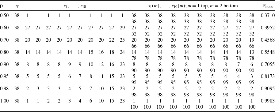

Figure 1. Success probability as a function of the number of queries K when $n=100$
objects and
$n=100$
objects and $M=2$
responses with symmetric probabilities
$M=2$
responses with symmetric probabilities $\mathsf{p}(1)=1-\mathsf{p}(2)=1-\mathsf{q}(1)=\mathsf{q}(2)=\mathsf{p}$
for
$\mathsf{p}(1)=1-\mathsf{p}(2)=1-\mathsf{q}(1)=\mathsf{q}(2)=\mathsf{p}$
for $\mathsf{p}=0.5,0.6,0.7,$ $0.8,0.9,0.95,0.98,1$
.
$0.8,0.9,0.95,0.98,1$
.
In Figure 1 we note the performance of the uniform case $\mathsf{p}=0.5$
which is constant, not changing with the number of queries. As we discussed, this is to be expected since, under the uniform model, expert responses contain no information. It is interesting in this case to compare our optimal scheme to the optimal scheme of the classical version. In the classical case with no queries we recall that the optimal search strategy consists in stopping the first time, but no sooner than
$\mathsf{p}=0.5$
which is constant, not changing with the number of queries. As we discussed, this is to be expected since, under the uniform model, expert responses contain no information. It is interesting in this case to compare our optimal scheme to the optimal scheme of the classical version. In the classical case with no queries we recall that the optimal search strategy consists in stopping the first time, but no sooner than $r_{\textrm{f}}=38$
, that we observe
$r_{\textrm{f}}=38$
, that we observe $z_t=1$
. When we allow queries with
$z_t=1$
. When we allow queries with $\mathsf{p}=0.5$
, as we can see, the querying thresholds
$\mathsf{p}=0.5$
, as we can see, the querying thresholds $r_1 ,\ldots , r_K$
are all equal to 1. This means that the first K times we encounter a relative rank equal to
$r_1 ,\ldots , r_K$
are all equal to 1. This means that the first K times we encounter a relative rank equal to $z_t=1$
we must query. However, stopping at any of the querying times happens only if the querying time is no smaller than
$z_t=1$
we must query. However, stopping at any of the querying times happens only if the querying time is no smaller than $s_k(m)=r_{\textrm{f}}=38$
. If all K queries are exhausted before time 38, then we use the terminal time
$s_k(m)=r_{\textrm{f}}=38$
. If all K queries are exhausted before time 38, then we use the terminal time $\mathcal{T}_{\textrm{f}}$
that has a threshold equal to
$\mathcal{T}_{\textrm{f}}$
that has a threshold equal to $r_{\textrm{f}}=38$
as well. Consequently, final-stopping occurs if we encounter a rank equal to 1 no sooner than
$r_{\textrm{f}}=38$
as well. Consequently, final-stopping occurs if we encounter a rank equal to 1 no sooner than $r_{\textrm{f}}$
. Combining carefully all the possibilities we conclude that we stop at the first time after and including
$r_{\textrm{f}}$
. Combining carefully all the possibilities we conclude that we stop at the first time after and including $r_{\textrm{f}}$
that we encounter a rank equal to 1. In other words, we match the classical optimal scheme.
$r_{\textrm{f}}$
that we encounter a rank equal to 1. In other words, we match the classical optimal scheme.
In the last row of Table 2 we have the case of an infallible expert. We know that the optimal decision with an infallible expert requires the termination of the search if the expert responds with ‘ $\{\xi_t=1\}$
’ and continuation of the search if the response is ‘
$\{\xi_t=1\}$
’ and continuation of the search if the response is ‘ $\{\xi_t>1\}$
’. In our setup, instead, we compare the querying time
$\{\xi_t>1\}$
’. In our setup, instead, we compare the querying time $\mathcal{T}_k$
to the threshold
$\mathcal{T}_k$
to the threshold $s_k(m)$
. From the table we see that
$s_k(m)$
. From the table we see that $s_k(1)=1$
,
$s_k(1)=1$
, $s_k(2)=n$
for all
$s_k(2)=n$
for all $k=1,\ldots,K$
. According to our model,
$k=1,\ldots,K$
. According to our model, $\zeta_{\mathcal{T}_k}=1$
corresponds with certainty (because
$\zeta_{\mathcal{T}_k}=1$
corresponds with certainty (because $\mathsf{p}=1$
) to
$\mathsf{p}=1$
) to $\xi_{\mathcal{T}_k}=1$
, and therefore if
$\xi_{\mathcal{T}_k}=1$
, and therefore if $\zeta_{\mathcal{T}_k}=1$
we see that we necessarily stop at
$\zeta_{\mathcal{T}_k}=1$
we see that we necessarily stop at $\mathcal{T}_k$
since
$\mathcal{T}_k$
since $\mathcal{T}_k\geq s_k(1)=1$
. On the other hand,
$\mathcal{T}_k\geq s_k(1)=1$
. On the other hand, $\zeta_{\mathcal{T}_k}=2$
corresponds with certainty to
$\zeta_{\mathcal{T}_k}=2$
corresponds with certainty to $\xi_{\mathcal{T}_k}>1$
, and when
$\xi_{\mathcal{T}_k}>1$
, and when $\zeta_{\mathcal{T}_k}=2$
occurs we can stop only if
$\zeta_{\mathcal{T}_k}=2$
occurs we can stop only if $\mathcal{T}_k\geq s_k(2)=n$
which is impossible (unless
$\mathcal{T}_k\geq s_k(2)=n$
which is impossible (unless $\mathcal{T}_k=n$
, where we necessarily stop since we have exhausted all objects). Therefore, when
$\mathcal{T}_k=n$
, where we necessarily stop since we have exhausted all objects). Therefore, when $\mathsf{p}=1$
our optimal scheme matches the optimal scheme of an infallible expert. This can be further corroborated by comparing our thresholds
$\mathsf{p}=1$
our optimal scheme matches the optimal scheme of an infallible expert. This can be further corroborated by comparing our thresholds $r_{\textrm{f}}=38$
and
$r_{\textrm{f}}=38$
and $r_{10}=23$
with the corresponding thresholds
$r_{10}=23$
with the corresponding thresholds $s^*,r^*$
in [Reference Gilbert and Mosteller9, Table∼3] and verifying that they are the same with the same success probability (in [Reference Gilbert and Mosteller9], there are tables only for
$s^*,r^*$
in [Reference Gilbert and Mosteller9, Table∼3] and verifying that they are the same with the same success probability (in [Reference Gilbert and Mosteller9], there are tables only for $K=0,1$
).
$K=0,1$
).
From Figure 1 we can also observe the fact we described in Remark 6, namely that there is an improvement in the success probability; however, the optimal value ‘saturates’ with the limiting value being strictly less than 1. An additional conclusion we can draw from this example is that the thresholds also converge to some limiting value. This means that, after some point, increasing K results in repeating the last thresholds and experiencing the same optimal performance. The only case which does not follow this rule and the probability of success converges to 1 as the number of queries increases is when $\mathsf{p}=1$
, which, as mentioned, corresponds to an infallible expert.
$\mathsf{p}=1$
, which, as mentioned, corresponds to an infallible expert.
A final observation regarding our example is the case where the value of the parameter $\mathsf{p}$
satisfies
$\mathsf{p}$
satisfies $\mathsf{p}<0.5$
. Using the formulas of Table 1 we can show that we obtain exactly the same results as using, instead of
$\mathsf{p}<0.5$
. Using the formulas of Table 1 we can show that we obtain exactly the same results as using, instead of $\mathsf{p}$
, the value
$\mathsf{p}$
, the value $1-\mathsf{p}>0.5$
. The only modification we need to make is to exchange the roles of
$1-\mathsf{p}>0.5$
. The only modification we need to make is to exchange the roles of $m=1$
and
$m=1$
and $m=2$
in the thresholds
$m=2$
in the thresholds $s_k(m)$
. We can see why this modification is necessary by considering the extreme case
$s_k(m)$
. We can see why this modification is necessary by considering the extreme case $\mathsf{p}=0$
corresponding to
$\mathsf{p}=0$
corresponding to $\mathbb{P}(\zeta_t=1\mid\xi_t=1)=0$
. Then, when
$\mathbb{P}(\zeta_t=1\mid\xi_t=1)=0$
. Then, when $M=2$
, it is of course true that
$M=2$
, it is of course true that $\mathbb{P}(\zeta_t=2\mid\xi_t=1)=1$
and, therefore, we now have that the value
$\mathbb{P}(\zeta_t=2\mid\xi_t=1)=1$
and, therefore, we now have that the value $\zeta_t=2$
corresponds with certainty to
$\zeta_t=2$
corresponds with certainty to $\{\xi_t=1\}$
. This exchange of roles between
$\{\xi_t=1\}$
. This exchange of roles between $m=1$
and
$m=1$
and $m=2$
continues to apply when
$m=2$
continues to apply when $0\leq\mathsf{p}<0.5$
.
$0\leq\mathsf{p}<0.5$
.
Appendix
Proof of Lemma
1. The validity of (2) is well known for any collection of values $\{\xi_t,\ldots,\xi_1\}$
under the uniform model without replacement, since
$\{\xi_t,\ldots,\xi_1\}$
under the uniform model without replacement, since $\xi_\ell$
takes one of
$\xi_\ell$
takes one of $n-\ell+1$
values, each with the same probability
$n-\ell+1$
values, each with the same probability ${1}/({n-\ell+1})$
. Suppose now that the collection
${1}/({n-\ell+1})$
. Suppose now that the collection $\{\xi_t,\ldots,\xi_1\}$
, when occurring sequentially, produces the sequence of ranks
$\{\xi_t,\ldots,\xi_1\}$
, when occurring sequentially, produces the sequence of ranks $\{z_t,\ldots,z_1\}$
where
$\{z_t,\ldots,z_1\}$
where $1\leq z_t\leq t\leq n$
. If we fix a collection
$1\leq z_t\leq t\leq n$
. If we fix a collection $\{z_t,\ldots,z_1\}$
of t ranks, making sure that they conform with the constraint
$\{z_t,\ldots,z_1\}$
of t ranks, making sure that they conform with the constraint $1\leq z_\ell\leq \ell$
, and also select t integers
$1\leq z_\ell\leq \ell$
, and also select t integers $1\leq i_1<i_2<\cdots<i_t\leq n$
as possible object values, then there is a unique way to assign these values to
$1\leq i_1<i_2<\cdots<i_t\leq n$
as possible object values, then there is a unique way to assign these values to $\{\xi_t,\ldots,\xi_1\}$
in order to produce the specified ranks. Indeed, we start with
$\{\xi_t,\ldots,\xi_1\}$
in order to produce the specified ranks. Indeed, we start with $\xi_t$
, to which we assign the
$\xi_t$
, to which we assign the $z_t$
th value from the set
$z_t$
th value from the set $\{i_1,\ldots,i_t\}$
, that is, the value
$\{i_1,\ldots,i_t\}$
, that is, the value $i_{z_t}$
. We remove this element from the set of values and then we proceed to
$i_{z_t}$
. We remove this element from the set of values and then we proceed to $\xi_{t-1}$
to which we assign the
$\xi_{t-1}$
to which we assign the $z_{t-1}$
th element from the new list of values, etc. This procedure generates the specified ranks from any subset of
$z_{t-1}$
th element from the new list of values, etc. This procedure generates the specified ranks from any subset of $\{1,\ldots,n\}$
of size t.
$\{1,\ldots,n\}$
of size t.
As we just mentioned, for fixed ranks $\{z_t,\ldots,z_1\}$
, any subset of t integers from the set
$\{z_t,\ldots,z_1\}$
, any subset of t integers from the set $\{1,\ldots,n\}$
can be uniquely rearranged and assigned to
$\{1,\ldots,n\}$
can be uniquely rearranged and assigned to $\{\xi_t,\ldots,\xi_1\}$
in order to generate the specified rank sequence. There are
$\{\xi_t,\ldots,\xi_1\}$
in order to generate the specified rank sequence. There are $\binom{n}{t}$
such possible combinations with each combination having a probability of occurrence equal to
$\binom{n}{t}$
such possible combinations with each combination having a probability of occurrence equal to ${(n-t)!}/{n!}$
. Multiplying the two quantities yields the second equality in (2), from which we can then deduce that
${(n-t)!}/{n!}$
. Multiplying the two quantities yields the second equality in (2), from which we can then deduce that $\mathbb{P}(z_t\mid\mathscr{Z}_{t-1})={\mathbb{P}(z_t,\ldots,z_1)} / {\mathbb{P}(z_{t-1},\ldots,z_1)} = {1}/{t}$
and prove the third equality in (2).
$\mathbb{P}(z_t\mid\mathscr{Z}_{t-1})={\mathbb{P}(z_t,\ldots,z_1)} / {\mathbb{P}(z_{t-1},\ldots,z_1)} = {1}/{t}$
and prove the third equality in (2).
Consider now (3). If $\xi_{t_1}=1$
this forces
$\xi_{t_1}=1$
this forces $z_{t_1}=1$
and all ranks for times larger than
$z_{t_1}=1$
and all ranks for times larger than $t_1$
to be necessarily larger than 1. This is expressed through the indicator
$t_1$
to be necessarily larger than 1. This is expressed through the indicator $\textbf{1}_{\{z_{t_1}=1\}}\mathbb{1}_{t_1+1}^t = \textbf{1}_{\{z_{t_1}=1\}}\big(\prod_{\ell=t_1+1}^t\textbf{1}_{\{z_\ell>1\}}\big)$
. With
$\textbf{1}_{\{z_{t_1}=1\}}\mathbb{1}_{t_1+1}^t = \textbf{1}_{\{z_{t_1}=1\}}\big(\prod_{\ell=t_1+1}^t\textbf{1}_{\{z_\ell>1\}}\big)$
. With $\xi_{t_1}=1$
and
$\xi_{t_1}=1$
and $z_{t_1}=1$
let us fix the remaining ranks in
$z_{t_1}=1$
let us fix the remaining ranks in $\mathscr{Z}_t$
, assuring they are consistent with the constraint imposed for times larger than
$\mathscr{Z}_t$
, assuring they are consistent with the constraint imposed for times larger than $t_1$
and also recalling that
$t_1$
and also recalling that $z_\ell$
must take values in the set
$z_\ell$
must take values in the set $\{1,\ldots,\ell\}$
. We can now see that we are allowed to select the values of
$\{1,\ldots,\ell\}$
. We can now see that we are allowed to select the values of $t-1$
objects from a pool of
$t-1$
objects from a pool of $n-1$
integers (since the value 1 is already assigned to
$n-1$
integers (since the value 1 is already assigned to $\xi_{t_1}$
). This generates
$\xi_{t_1}$
). This generates $\binom{n-1}{t-1}$
combinations, and each combination, including also the fact that
$\binom{n-1}{t-1}$
combinations, and each combination, including also the fact that $\xi_{t_1}=1$
, has a probability of occurrence equal to
$\xi_{t_1}=1$
, has a probability of occurrence equal to ${(n-t)!}/{n!}$
. If we multiply the two quantities then we obtain (3). Applying (3) for
${(n-t)!}/{n!}$
. If we multiply the two quantities then we obtain (3). Applying (3) for $t_1=t$
(possible since
$t_1=t$
(possible since $t\geq t_1$
) and using the fact that by definition
$t\geq t_1$
) and using the fact that by definition $\mathbb{1}_{t+1}^t=1$
, we obtain (4). This concludes the proof of the lemma.
$\mathbb{1}_{t+1}^t=1$
, we obtain (4). This concludes the proof of the lemma.
Proof of Lemma 2. We begin with (5), and we note that
 \begin{equation} \mathbb{P}(\xi_t=1\mid\mathscr{Z}_t^k) = \frac{\mathbb{P}(\xi_t=1,\mathscr{Z}_t^k)}{\mathbb{P}(\mathscr{Z}_t^k)} = \frac{\mathbb{P}(\xi_t=1,\mathscr{Z}_t^k)}{\mathbb{P}(\mathscr{Z}_t^k)}\textbf{1}_{\{z_t=1\}}, \end{equation}
where the last equality is due to the fact that $\xi_t=1$
forces
$\xi_t=1$
forces $z_t$
to become 1 as well, and therefore the numerator is 0 if
$z_t$
to become 1 as well, and therefore the numerator is 0 if $z_t\neq1$
. This property is captured with the indicator
$z_t\neq1$
. This property is captured with the indicator $\textbf{1}_{\{z_t=1\}}$
. We can now write
$\textbf{1}_{\{z_t=1\}}$
. We can now write
 \begin{align*} \mathbb{P}(\xi_t=1,\mathscr{Z}_t^k) & = \mathbb{P}(\xi_t=1,\mathscr{Z}_{t}^k,\xi_{t_k}=1) + \mathbb{P}(\xi_t=1,\mathscr{Z}_{t}^k,\xi_{t_k}>1) \\[5pt] & = \mathbb{P}(\xi_t=1,\mathscr{Z}_{t}^k,\xi_{t_k}>1) \\[5pt] & =\mathbb{P}(\xi_t=1,\zeta_{t_k},\mathscr{Z}_{t}^{k-1},\xi_{t_k}>1) \\[5pt] & = \mathbb{P}(\xi_t=1,\zeta_{t_k},\mathscr{Z}_{t}^{k-1}\mid\xi_{t_k}>1)\mathbb{P}(\xi_{t_k}>1) \\[5pt] & = \mathbb{P}(\zeta_{t_k}\mid\xi_{t_k}>1) \mathbb{P}(\xi_t=1,\mathscr{Z}_{t}^{k-1}\mid\xi_{t_k}>1)\mathbb{P}(\xi_{t_k}>1) \\[5pt] & = \mathsf{q}(\zeta_{t_k})\mathbb{P}(\xi_t=1,\mathscr{Z}_{t}^{k-1},\xi_{t_k}>1) \\[5pt] & = \mathsf{q}(\zeta_{t_k})\{\mathbb{P}(\xi_t=1,\mathscr{Z}_{t}^{k-1}) - \mathbb{P}(\xi_t=1,\mathscr{Z}_{t}^{k-1},\xi_{t_k}=1)\} \\[5pt] & = \mathsf{q}(\zeta_{t_k})\mathbb{P}(\xi_t=1,\mathscr{Z}_{t}^{k-1}), \end{align*}
where $\mathsf{q}(\zeta_{t_k})$
, following the model in (1), denotes the probability of the expert responding with the value
$\mathsf{q}(\zeta_{t_k})$
, following the model in (1), denotes the probability of the expert responding with the value $\zeta_{t_k}$
given that
$\zeta_{t_k}$
given that $\xi_{t_k}>1$
. We also observe that the second and last equalities are true due to the fact that the fourth is impossible for two objects at different time instances to have the same value, while the fourth equality is true because, according to our model, when we condition on
$\xi_{t_k}>1$
. We also observe that the second and last equalities are true due to the fact that the fourth is impossible for two objects at different time instances to have the same value, while the fourth equality is true because, according to our model, when we condition on $\{\xi_{t_k}>1\}$
then
$\{\xi_{t_k}>1\}$
then $\zeta_{t_k}$
is independent of all ranks, other responses, and other object values.
$\zeta_{t_k}$
is independent of all ranks, other responses, and other object values.
In order to modify the denominator in (19), due to the indicator $\textbf{1}_{\{z_t=1\}}$
in the numerator it is sufficient to analyze the denominator by fixing
$\textbf{1}_{\{z_t=1\}}$
in the numerator it is sufficient to analyze the denominator by fixing $z_t=1$
. Specifically,
$z_t=1$
. Specifically,
 \begin{align*} \mathbb{P}(\mathscr{Z}_{t}^k,z_t=1) & = \mathbb{P}(\mathscr{Z}_{t}^k,z_t=1,\xi_{t_k}=1) + \mathbb{P}(\mathscr{Z}_{t}^k,z_t=1,\xi_{t_k}>1) \\[5pt] & = \mathbb{P}(\mathscr{Z}_{t}^k,z_t=1,\xi_{t_k}>1) \\[5pt] & = \mathbb{P}(\zeta_{t_k},\mathscr{Z}_{t}^{k-1},z_t=1,\xi_{t_k}>1) \\[5pt] & = \mathbb{P}(\zeta_{t_k}\mid\xi_{t_k}>1)\mathbb{P}(\mathscr{Z}_{t}^{k-1},z_t=1,\xi_{t_k}>1) \\[5pt] & = \mathsf{q}(\zeta_{t_k})\{\mathbb{P}(\mathscr{Z}_{t}^{k-1},z_t=1) - \mathbb{P}(\mathscr{Z}_{t}^{k-1},z_t=1,\xi_{t_k}=1)\} \\[5pt] & = \mathsf{q}(\zeta_{t_k})\mathbb{P}(z_t=1,\mathscr{Z}_{t}^{k-1}), \end{align*}
where in the third and the last equalities we used the fact that for $t>t_k$
we cannot have
$t>t_k$
we cannot have $z_t=1$
when
$z_t=1$
when $\xi_{t_k}=1$
because this requires
$\xi_{t_k}=1$
because this requires $\xi_t<\xi_{t_k}$
which is impossible since
$\xi_t<\xi_{t_k}$
which is impossible since $\xi_{t_k}=1$
. Dividing the numerator by the denominator proves that
$\xi_{t_k}=1$
. Dividing the numerator by the denominator proves that
 \begin{equation*} \mathbb{P}(\xi_t=1\mid\mathscr{Z}_t^k) = \frac{\mathbb{P}(\xi_t=1,\mathscr{Z}_{t}^{k-1})}{\mathbb{P}(z_t=1,\mathscr{Z}_{t}^{k-1})}\textbf{1}_{\{z_t=1\}} = \frac{\mathbb{P}(\xi_t=1,\mathscr{Z}_t^{k-1})}{\mathbb{P}(\mathscr{Z}_t^{k-1})}\textbf{1}_{\{z_t=1\}} = \mathbb{P}(\xi_t=1\mid\mathscr{Z}_t^{k-1})\textbf{1}_{\{z_t=1\}}. \end{equation*}
In other words, given that a new relatively best object appears, the probability that it is the best of all the objects is conditionally independent of the previous expert response. Applying this equality repeatedly, we conclude that
 \begin{equation} \mathbb{P}(\xi_t=1\mid\mathscr{Z}_t^k) = \mathbb{P}(\xi_t=1\mid\mathscr{Z}_t^0)\textbf{1}_{\{z_t=1\}} = \mathbb{P}(\xi_t=1\mid\mathscr{Z}_t)\textbf{1}_{\{z_t=1\}}, \end{equation}
namely, the conditional probability is independent of all past expert responses. Combining the second equality in (2) with (4), we can now show that
 \begin{align*} \mathbb{P}(\xi_t=1\mid\mathscr{Z}_t) = \frac{\mathbb{P}(\xi_t=1,\mathscr{Z}_t)}{\mathbb{P}(\mathscr{Z}_t)} = \frac{({1}/({(t-1)!n}))\textbf{1}_{\{z_t=1\}}}{{1}/{t!}} = \frac{t}{n}\textbf{1}_{\{z_t=1\}}, \end{align*}
which, if substituted into (20), proves (5) and suggests that the desired conditional probability $\mathbb{P}(\xi_t=1\mid\mathscr{Z}_t^k)$
depends only on t and
$\mathbb{P}(\xi_t=1\mid\mathscr{Z}_t^k)$
depends only on t and $z_t$
and not on
$z_t$
and not on $\mathscr{Z}_{t-1}^k$
, namely the previous ranks and previous expert responses.
$\mathscr{Z}_{t-1}^k$
, namely the previous ranks and previous expert responses.
To show (6) we observe that
 \begin{align*} \mathbb{P}(\xi_{t_k}=1\mid\mathscr{Z}_{t_k}^k) = \frac{\mathbb{P}(\xi_{t_k}=1,\mathscr{Z}_{t_k}^k)}{\mathbb{P}(\mathscr{Z}_{t_k}^k)}. \end{align*}
For the numerator, using similar steps to before, we can write
 \begin{align*} \mathbb{P}(\xi_{t_k}=1,\mathscr{Z}_{t_k}^k) & = \mathbb{P}(\xi_{t_k}=1,\zeta_{t_k},\mathscr{Z}_{t_k}^{k-1}) \\[5pt] & = \mathsf{p}(\zeta_{t_k})\mathbb{P}(\xi_{t_k}=1,\mathscr{Z}_{t_k}^{k-1}) \\[5pt] & = \mathsf{p}(\zeta_{t_k})\mathbb{P}(\xi_{t_k}=1\mid\mathscr{Z}_{t_k}^{k-1})\mathbb{P}(\mathscr{Z}_{t_k}^{k-1}) \\[5pt] & = \mathsf{p}(\zeta_{t_k})\frac{t_k}{n}\textbf{1}_{\{z_{t_k}=1\}}\mathbb{P}(\mathscr{Z}_{t_k}^{k-1}), \end{align*}
where for the second equality we first conditioned on $\{\xi_{t_k}=1\}$
and used the fact that
$\{\xi_{t_k}=1\}$
and used the fact that $\zeta_{t_k}$
is independent of any other information, while for the last equality we applied (5).
$\zeta_{t_k}$
is independent of any other information, while for the last equality we applied (5).
Similarly, for the denominator we have
 \begin{align} \mathbb{P}(\mathscr{Z}_{t_k}^k) & = \mathbb{P}(\zeta_{t_k},\mathscr{Z}_{t_k}^{k-1}) \nonumber \\[5pt] & = \mathbb{P}(\xi_{t_k}=1,\zeta_{t_k},\mathscr{Z}_{t_k}^{k-1}) + \mathbb{P}(\xi_{t_k}>1,\zeta_{t_k},\mathscr{Z}_{t_k}^{k-1}) \nonumber \\[5pt] & = \mathsf{p}(\zeta_{t_k})\mathbb{P}(\xi_{t_k}=1,\mathscr{Z}_{t_k}^{k-1}) + \mathsf{q}(\zeta_{t_k})\mathbb{P}(\xi_{t_k}>1,\mathscr{Z}_{t_k}^{k-1}) \nonumber \\[5pt] & = \{\mathsf{p}(\zeta_{t_k})\mathbb{P}(\xi_{t_k}=1\mid\mathscr{Z}_{t_k}^{k-1}) + \mathsf{q}(\zeta_{t_k})\mathbb{P}(\xi_{t_k}>1\mid\mathscr{Z}_{t_k}^{k-1})\} \mathbb{P}(\mathscr{Z}_{t_k}^{k-1}) \nonumber \\[5pt] & = \bigg\{\mathsf{p}(\zeta_{t_k})\frac{t_k}{n}\textbf{1}_{\{z_{t_k}=1\}} + \mathsf{q}(\zeta_{t_k})\bigg(1-\frac{t_k}{n}\textbf{1}_{\{z_{t_k}=1\}}\bigg)\bigg\} \mathbb{P}(\mathscr{Z}_{t_k}^{k-1}), \end{align}
where for the last equality we applied the same idea we used in the last equality of the numerator. Dividing the numerator by the denominator and using the fact that in the numerator we have the indicator $\textbf{1}_{\{z_{t_k}=1\}}$
, it is easy to verify that we obtain the expression appearing in (6).
$\textbf{1}_{\{z_{t_k}=1\}}$
, it is easy to verify that we obtain the expression appearing in (6).
To prove (7), we have
 \begin{align*} \mathbb{P}(\zeta_{t_k}\mid\mathscr{Z}_{t_k}^{k-1},z_{t_k}=1) & = \frac{\mathbb{P}(\zeta_{t_k},\mathscr{Z}_{t_k}^{k-1},z_{t_k}=1)}{\mathbb{P}(\mathscr{Z}_{t_k}^{k-1},z_{t_k}=1)} \\[5pt] & = \frac{\mathbb{P}(\mathscr{Z}_{t_k}^{k},z_{t_k}=1)}{\mathbb{P}(\mathscr{Z}_{t_k}^{k-1},z_{t_k}=1)} = \mathsf{p}(\zeta_{t_k})\frac{t_k}{n}+\mathsf{q}(\zeta_{t_k})\bigg(1-\frac{t_k}{n}\bigg), \end{align*}
where for the last equality we used (21) and applied it for $z_{t_k}=1$
.
$z_{t_k}=1$
.
Let us now demonstrate (8), which is the relationship that distinguishes our random model from the classical infallible expert case. We observe that
 \begin{align*} \mathbb{P}(z_t=1\mid\mathscr{Z}_{t-1}^k,z_{t_k}=1) = \frac{\mathbb{P}(z_t=1,\mathscr{Z}_{t-1},z_{t_k}=1,\zeta_{t_k},\ldots,\zeta_{t_1})} {\mathbb{P}(\mathscr{Z}_{t-1},z_{t_k}=1,\zeta_{t_k},\ldots,\zeta_{t_1})}. \end{align*}
As before, for the numerator we can write
 \begin{align*} \mathbb{P}(z_t=1,\mathscr{Z}_{t-1},z_{t_k}=1,\zeta_{t_k},\ldots,\zeta_{t_1}) & = \mathbb{P}(z_t=1,\mathscr{Z}_{t-1},z_{t_k}=1,\zeta_{t_k},\ldots,\zeta_{t_1},\xi_{t_1}>1) \\[5pt] & = \mathbb{P}(z_t=1,\mathscr{Z}_{t-1},z_{t_k}=1,\zeta_{t_k},\ldots,\zeta_{t_2},\xi_{t_1}>1)\mathsf{q}(\zeta_{t_1})\\[5pt] & = \mathbb{P}(z_t=1,\mathscr{Z}_{t-1},z_{t_k}=1,\zeta_{t_k},\ldots,\zeta_{t_2})\mathsf{q}(\zeta_{t_1}). \end{align*}
For the denominator, due to the constraint $z_{t_k}=1$
, we can follow similar steps to the numerator and show that
$z_{t_k}=1$
, we can follow similar steps to the numerator and show that
 \begin{align*} \mathbb{P}(\mathscr{Z}_{t-1},z_{t_k}=1,\zeta_{t_k},\ldots,\zeta_{t_1}) = \mathbb{P}(\mathscr{Z}_{t-1},z_{t_k}=1,\zeta_{t_k},\ldots,\zeta_{t_2})\mathsf{q}(\zeta_{t_1}). \end{align*}
Dividing the numerator by the denominator yields
 \begin{align*} \frac{\mathbb{P}(z_t=1,\mathscr{Z}_{t-1},z_{t_k}=1,\zeta_{t_k},\ldots,\zeta_{t_1})} {\mathbb{P}(\mathscr{Z}_{t-1},z_{t_k}=1,\zeta_{t_k},\ldots,\zeta_{t_1})} = \frac{\mathbb{P}(z_t=1,\mathscr{Z}_{t-1},z_{t_k}=1,\zeta_{t_k},\ldots,\zeta_{t_2})} {\mathbb{P}(\mathscr{Z}_{t-1},z_{t_k}=1,\zeta_{t_k},\ldots,\zeta_{t_2})}, \end{align*}
which suggests that the first ratio does not depend on $\zeta_{t_1}$
. Following similar steps we can remove all previous expert responses one by one, and prove that
$\zeta_{t_1}$
. Following similar steps we can remove all previous expert responses one by one, and prove that
 \begin{align*} \mathbb{P}(z_t=1\mid\mathscr{Z}_{t-1}^k,z_{t_k}=1) = \frac{\mathbb{P}(z_t=1,\mathscr{Z}_{t-1},z_{t_k}=1,\zeta_{t_k})}{\mathbb{P}(\mathscr{Z}_{t-1},z_{t_k}=1,\zeta_{t_k})}, \end{align*}
namely, the conditional probability depends only on the most recent expert response. It is possible now to obtain more suitable expressions for the numerator and the denominator. We start with the numerator and apply steps similar to above. Specifically,
 \begin{align*} \mathbb{P}(z_t=1,\mathscr{Z}_{t-1},z_{t_k}=1,\zeta_{t_k}) & = \mathbb{P}(z_t=1,\mathscr{Z}_{t-1},z_{t_k}=1,\zeta_{t_k},\xi_{t_k}>1) \\[5pt] & = \mathbb{P}(z_t=1,\mathscr{Z}_{t-1},z_{t_k}=1)\mathsf{q}(\zeta_{t_k}) = \frac{1}{t!}\mathsf{q}(\zeta_{t_k}), \end{align*}
where for the last expression we used the second equality in (2) after observing that $\{z_t=1,\mathscr{Z}_{t-1},z_{t_k}=1\}$
is simply
$\{z_t=1,\mathscr{Z}_{t-1},z_{t_k}=1\}$
is simply $\mathscr{Z}_t$
with two of its elements fixed to 1.
$\mathscr{Z}_t$
with two of its elements fixed to 1.
For the denominator, we can similarly write
 \begin{align*} \mathbb{P}(\mathscr{Z}_{t-1},z_{t_k}=1,\zeta_{t_k}) & = \mathbb{P}(\mathscr{Z}_{t-1},z_{t_k}=1,\zeta_{t_k},\xi_{t_k}=1) + \mathbb{P}(\mathscr{Z}_{t-1},z_{t_k}=1,\zeta_{t_k},\xi_{t_k}>1) \\[5pt] & = \mathbb{P}(\mathscr{Z}_{t-1},z_{t_k}=1,\xi_{t_k}=1)\mathsf{p}(\zeta_{t_k}) + \mathbb{P}(\mathscr{Z}_{t-1},z_{t_k}=1,\xi_{t_k}>1)\mathsf{q}(\zeta_{t_k}) \\[5pt] & = \mathbb{P}(\mathscr{Z}_{t-1},z_{t_k}=1,\xi_{t_k}=1)\mathsf{p}(\zeta_{t_k}) \\[5pt] & \quad + \{\mathbb{P}(\mathscr{Z}_{t-1},z_{t_k}=1) - \mathbb{P}(\mathscr{Z}_{t-1},z_{t_k}=1,\xi_{t_k}=1)\}\mathsf{q}(\zeta_{t_k}) \\[5pt] & = \bigg\{\frac{1}{(t-2)!n}\mathbb{1}_{t_k+1}^{t-1}\bigg\}\mathsf{p}(\zeta_{t_k}) + \bigg\{\frac{1}{(t-1)!}-\frac{1}{(t-2)!n}\mathbb{1}_{t_k+1}^{t-1}\bigg\}\mathsf{q}(\zeta_{t_k}), \end{align*}
where to obtain the last expression we applied the second equality of (2) combined with (3) after observing that by fixing $z_{t_k}=1$
the product
$z_{t_k}=1$
the product $\textbf{1}_{\{z_{t_k}=1\}}\mathbb{1}_{t_k+1}^{t-1}$
produced by (3) becomes
$\textbf{1}_{\{z_{t_k}=1\}}\mathbb{1}_{t_k+1}^{t-1}$
produced by (3) becomes $\mathbb{1}_{t_k+1}^{t-1}$
. Dividing the numerator by the denominator we can verify that the resulting ratio matches the right-hand side of (8) for the two possible values of
$\mathbb{1}_{t_k+1}^{t-1}$
. Dividing the numerator by the denominator we can verify that the resulting ratio matches the right-hand side of (8) for the two possible values of $\mathbb{1}_{t_k+1}^{t-1}$
, namely 0 or 1. This completes the proof of Lemma 2.
$\mathbb{1}_{t_k+1}^{t-1}$
, namely 0 or 1. This completes the proof of Lemma 2.
Proof of Theorem
1. We first note that $\mathbb{P}_{\mathsf{succ}}=\mathcal{P}_{K}$
, where
$\mathbb{P}_{\mathsf{succ}}=\mathcal{P}_{K}$
, where $\mathcal{P}_{K}$
satisfies (15) for
$\mathcal{P}_{K}$
satisfies (15) for $k=K$
and
$k=K$
and $\mathcal{U}_t^{K+1}={t}/{n}$
. Consider now the general form of
$\mathcal{U}_t^{K+1}={t}/{n}$
. Consider now the general form of $\mathcal{P}_k$
defined in (15). We focus on the last term, which we intend to optimize with respect to
$\mathcal{P}_k$
defined in (15). We focus on the last term, which we intend to optimize with respect to $\mathcal{T}_{k+1}$
. Observe that
$\mathcal{T}_{k+1}$
. Observe that
 \begin{align} \mathbb{E} &\Big[\mathcal{U}_{\mathcal{T}_{k+1}}^{k+1}\textbf{1}_{\{z_{\mathcal{T}_{k+1}}=1\}} \textbf{1}_{\mathscr{B}_{\mathcal{T}_1}^{\mathcal{T}_{k}}}\Big] \nonumber \\[5pt] & = \mathop{\sum^{n}\cdots\sum^{n}}_{t_k>\cdots>t_1>0}\mathbb{E}\Big[\mathcal{U}_{\mathcal{T}_{k+1}}^{k+1} \textbf{1}_{\{z_{\mathcal{T}_{k+1}}=1\}}\textbf{1}_{\{\mathcal{T}_{k+1}>t_k\}} \textbf{1}_{\{\mathcal{T}_k=t_k\}}\cdots\textbf{1}_{\{\mathcal{T}_1=t_1\}} \textbf{1}_{\mathscr{B}_{t_1}^{t_{k}}}\Big] \nonumber \\[5pt] & = \mathop{\sum^{n}\cdots\sum^{n}}_{t_k>\cdots>t_1>0}\mathbb{E}\Big[\mathbb{E}\big[ \mathcal{U}_{\mathcal{T}_{k+1}}^{k+1}\textbf{1}_{\{z_{\mathcal{T}_{k+1}}=1\}}\mid\mathscr{Z}_{t_k}^k\big] \textbf{1}_{\{\mathcal{T}_{k+1}>t_k\}}\textbf{1}_{\{\mathcal{T}_k=t_k\}}\cdots\textbf{1}_{\{\mathcal{T}_1=t_1\}} \textbf{1}_{\mathscr{B}_{t_1}^{t_{k}}}\Big], \end{align}
where, in the last equality, as we point out in Remark 3, the indicators $\textbf{1}_{\{\mathcal{T}_{k+1}>t_k\}}$
,
$\textbf{1}_{\{\mathcal{T}_{k+1}>t_k\}}$
, $\textbf{1}_{\{\mathcal{T}_k=t_k\}}$
, … ,
$\textbf{1}_{\{\mathcal{T}_k=t_k\}}$
, … , $\textbf{1}_{\{\mathcal{T}_1=t_1\}}$
,
$\textbf{1}_{\{\mathcal{T}_1=t_1\}}$
, $\textbf{1}_{\mathscr{B}_{t_1}^{t_{k}}}$
are measurable with respect to
$\textbf{1}_{\mathscr{B}_{t_1}^{t_{k}}}$
are measurable with respect to $\mathscr{Z}_{t_k}^k$
and, consequently, can be placed outside the inner expectation.
$\mathscr{Z}_{t_k}^k$
and, consequently, can be placed outside the inner expectation.
We could isolate the inner expectation and optimize it by solving the optimal stopping problem
 \begin{equation} \max_{\mathcal{T}_{k+1}>t_{k}}\mathbb{E}\big[\mathcal{U}_{\mathcal{T}_{k+1}}^{k+1} \textbf{1}_{\{z_{\mathcal{T}_{k+1}}=1\}}|\mathscr{Z}_{t_k}^k\big] \end{equation}
with respect to $\mathcal{T}_{k+1}$
. Unfortunately, the proposed optimization turns out to be unnecessarily involved, resulting in an optimal reward which is a complicated expression of the information
$\mathcal{T}_{k+1}$
. Unfortunately, the proposed optimization turns out to be unnecessarily involved, resulting in an optimal reward which is a complicated expression of the information $\mathscr{Z}_{t_k}^k$
. After careful examination, and recalling from (9) that
$\mathscr{Z}_{t_k}^k$
. After careful examination, and recalling from (9) that $\textbf{1}_{\mathscr{B}_{t_1}^{t_{k}}}$
contains the indicator
$\textbf{1}_{\mathscr{B}_{t_1}^{t_{k}}}$
contains the indicator $\textbf{1}_{\{z_{t_k}=1\}}$
, it is sufficient to consider the case where
$\textbf{1}_{\{z_{t_k}=1\}}$
, it is sufficient to consider the case where $z_{t_k}$
is fixed to the value 1. This constraint considerably simplifies our analysis and is the main reason we have developed the equalities (7) and (8) in Lemma 2. We also recall that
$z_{t_k}$
is fixed to the value 1. This constraint considerably simplifies our analysis and is the main reason we have developed the equalities (7) and (8) in Lemma 2. We also recall that $z_{t_k}=1$
, according to Remark 1, is a prerequisite for querying at
$z_{t_k}=1$
, according to Remark 1, is a prerequisite for querying at $t_k$
.
$t_k$
.
After this observation, we replace (22) with the alternative relationship
 \begin{align*}\mathbb{E}\Big[\mathcal{U}_{\mathcal{T}_{k+1}}^{k+1}\textbf{1}_{\{z_{\mathcal{T}_{k+1}}=1\}} \textbf{1}_{\mathscr{B}_{\mathcal{T}_1}^{\mathcal{T}_{k}}}\Big] = \,\,\,\,\,\,\,\,\,\,\,\,\,\,\,\,\,\,\,\,\,\,\,\,\,\,\,\,\,\,\,\,\,\,\,\,\,\,\,\,\,\,\,\,\,\,\,\,\,\,\,\,\,\,\,\,\,\,\,\,\,\,\,\,\,\,\,\,\,\,\,\,\,\,\,\,\,\,\,\,\,\,\,\,\,\,\,\,\,\,\,\,\,\,\,\,\,\,\,\,\,\,\,\,\,\,\,\,\,\,\,\,\,\,\,\,\,\,\,\,\,\,\,\,\,\,\,\,\,\,\,\,\,\,\,\,\,\,\,\,\,\,\,\,\,\,\,\,\,\,\,\,\,\\[5pt] \mathop{\sum^{n}\cdots\sum^{n}}_{t_k>\cdots>t_1>0}\mathbb{E}\Big[\mathbb{E}\big[ \mathcal{U}_{\mathcal{T}_{k+1}}^{k+1}\textbf{1}_{\{z_{\mathcal{T}_{k+1}}=1\}}\mid\mathscr{Z}_{t_k}^k,z_{t_k}=1\big] \textbf{1}_{\{\mathcal{T}_{k+1}>t_k\}}\textbf{1}_{\{\mathcal{T}_k=t_k\}}\cdots\textbf{1}_{\{\mathcal{T}_1=t_1\}} \textbf{1}_{\mathscr{B}_{t_1}^{t_{k}}}\Big]. \end{align*}
Again, we emphasize that we are allowed to make this specific conditioning because the value $z_{t_k}=1$
is imposed by the indicator
$z_{t_k}=1$
is imposed by the indicator $\textbf{1}_{\{z_{t_k}=1\}}$
contained in
$\textbf{1}_{\{z_{t_k}=1\}}$
contained in $\textbf{1}_{\mathscr{B}_{t_1}^{t_{k}}}$
. Let us now isolate the inner expectation in (24) and consider the following optimal stopping problem in place of (23):
$\textbf{1}_{\mathscr{B}_{t_1}^{t_{k}}}$
. Let us now isolate the inner expectation in (24) and consider the following optimal stopping problem in place of (23):
 \begin{equation} \max_{\mathcal{T}_{k+1}>t_{k}}\mathbb{E}\big[\mathcal{U}_{\mathcal{T}_{k+1}}^{k+1} \textbf{1}_{\{z_{\mathcal{T}_{k+1}}=1\}}\mid\mathscr{Z}_{t_k}^k,z_{t_k}=1\big]. \end{equation}
Following [Reference Peskir and Shiryaev17, Reference Shiryaev20], for $t>t_k$
we need to define the sequence of optimal rewards
$t>t_k$
we need to define the sequence of optimal rewards $\{\mathcal{R}_t^k\}$
, where
$\{\mathcal{R}_t^k\}$
, where
 \begin{equation} \mathcal{R}_t^k = \max_{\mathcal{T}_{k+1}\geq t}\mathbb{E}\big[\mathcal{U}_{\mathcal{T}_{k+1}}^{k+1} \textbf{1}_{\{z_{\mathcal{T}_{k+1}}=1\}}\mid\mathscr{Z}_t^k,z_{t_k}=1\big]. \end{equation}
From optimal stopping theory we have that $\{\mathcal{R}_t^{k}\}$
satisfies the backward recursion
$\{\mathcal{R}_t^{k}\}$
satisfies the backward recursion
 \begin{equation} \mathcal{R}_t^k = \max\big\{\mathcal{U}_t^{k+1}\textbf{1}_{\{z_t=1\}}, \mathbb{E}\big[\mathcal{R}_{t+1}^k\mid\mathscr{Z}_t^k,z_{t_k}=1\big]\big\}, \end{equation}
which must be applied for $t=n,n-1,\ldots,t_k+1$
and initialized with
$t=n,n-1,\ldots,t_k+1$
and initialized with $\mathcal{R}_{n+1}^k=0$
. We recall that
$\mathcal{R}_{n+1}^k=0$
. We recall that $t_k$
is excluded from the possible values of
$t_k$
is excluded from the possible values of $\mathcal{T}_{k+1}$
since we require
$\mathcal{T}_{k+1}$
since we require $\mathcal{T}_{k+1}>t_k$
.
$\mathcal{T}_{k+1}>t_k$
.
In order to find an explicit formula for the reward, we use the definition of the sequence $\{\mathcal{A}_t^k\}$
from (13) and we introduce a second sequence
$\{\mathcal{A}_t^k\}$
from (13) and we introduce a second sequence $\{\mathcal{B}_{t}^k(m)\}$
satisfying the backward recursion
$\{\mathcal{B}_{t}^k(m)\}$
satisfying the backward recursion
 \begin{align} \mathcal{B}_{t-1}^k(m) & = \mathcal{B}_{t}^k(m)\bigg(1-\frac{1}{t}\bigg) \nonumber \\[5pt] & \quad + \big(\mathcal{A}_t^k\!+\!\mathcal{B}_{t}^k(m)-\max\{\mathcal{U}_t^{k+1},\mathcal{A}_t^k\}\big) \frac{1}{t}\frac{\big(\mathsf{p}(m)-\mathsf{q}(m)\big)(t-1)}{\mathsf{p}(m)(t-1)+\mathsf{q}(m)(n-t+1)}, \end{align} $t=n,\ldots,t_k$
,
$t=n,\ldots,t_k$
, $m=1,\ldots,M$
, which is initialized with
$m=1,\ldots,M$
, which is initialized with $\mathcal{B}_{n}^k(m)=0$
. Actually, we are interested in the expected reward
$\mathcal{B}_{n}^k(m)=0$
. Actually, we are interested in the expected reward $\mathcal{V}_{t}^k = \mathbb{E}[\mathcal{R}_{t+1}^k\mid\mathscr{Z}_t^k,z_{t_k}=1]$
for which we intend to show, using (backward) induction, that
$\mathcal{V}_{t}^k = \mathbb{E}[\mathcal{R}_{t+1}^k\mid\mathscr{Z}_t^k,z_{t_k}=1]$
for which we intend to show, using (backward) induction, that
 \begin{equation} \mathcal{V}_{t}^k=\mathcal{A}_t^k+\mathcal{B}_{t}^k(\zeta_{t_k})\mathbb{1}_{t_{k}+1}^t. \end{equation}
Indeed, we have that (29) is true for $t=n$
since both the right- and left-hand sides are 0. Assume our claim is true for t; then we will show that it is also valid for
$t=n$
since both the right- and left-hand sides are 0. Assume our claim is true for t; then we will show that it is also valid for $t-1$
. Using (27) we can write
$t-1$
. Using (27) we can write
 \begin{align*} \mathcal{R}_{t}^k & = \max\{\mathcal{U}_t^{k+1},\mathcal{V}_{t}^k\}\textbf{1}_{\{z_t=1\}}+\mathcal{V}_{t}^k\textbf{1}_{\{z_t>1\}} \\[5pt] & = \max\{\mathcal{U}_t^{k+1},\mathcal{A}_t^k+\mathcal{B}_{t}^k(\zeta_{t_k})\mathbb{1}_{t_{k}+1}^t\} \textbf{1}_{\{z_t=1\}} + \big(\mathcal{A}_t^k+\mathcal{B}_{t}^k(\zeta_{t_k})\mathbb{1}_{t_{k}+1}^t\big)\textbf{1}_{\{z_t>1\}} \\[5pt] & = \max\{\mathcal{U}_t^{k+1},\mathcal{A}_t^k\}\textbf{1}_{\{z_t=1\}} + \big(\mathcal{A}_t^k+\mathcal{B}_{t}^k(\zeta_{t_k})\mathbb{1}_{t_{k}+1}^{t-1}\big)\textbf{1}_{\{z_t>1\}}. \end{align*}
Taking expectations on both sides conditioned on $\{\mathscr{Z}_{t-1}^k,z_{t_k}=1\}$
, using (8), and rearranging terms, it is not complicated to verify that
$\{\mathscr{Z}_{t-1}^k,z_{t_k}=1\}$
, using (8), and rearranging terms, it is not complicated to verify that $\mathcal{V}_{t-1}^k$
is also equal to
$\mathcal{V}_{t-1}^k$
is also equal to $\mathcal{A}_{t-1}^k+\mathcal{B}_{t-1}^k(\zeta_{t_k})\mathbb{1}_{t_{k}+1}^{t-1}$
, provided that
$\mathcal{A}_{t-1}^k+\mathcal{B}_{t-1}^k(\zeta_{t_k})\mathbb{1}_{t_{k}+1}^{t-1}$
, provided that $\{\mathcal{A}_t^k\}$
and
$\{\mathcal{A}_t^k\}$
and $\{\mathcal{B}_{t}^k(m)\}$
are defined by (13) and (28), respectively.
$\{\mathcal{B}_{t}^k(m)\}$
are defined by (13) and (28), respectively.
Let us now return to the optimization problem in (25). According to our analysis, the optimal reward satisfies
 \begin{equation} \max_{\mathcal{T}_{k+1}>t_k}\mathbb{E}\big[\mathcal{U}_{\mathcal{T}_{k+1}}^{k+1}\textbf{1}_{\{z_{\mathcal{T}_{k+1}}=1\}}\mid \mathscr{Z}_{t_k}^k,z_{t_k}=1\big] = \mathcal{V}_{t_k}^k = \mathcal{A}_{t_k}^k + \mathcal{B}_{t_k}^k(\zeta_{t_k})\mathbb{1}_{t_{k}+1}^{t_{k}} = \mathcal{A}_{t_{k}}^k + \mathcal{B}_{t_{k}}^k(\zeta_{t_k}), \end{equation}
since, according to our definition, $\mathbb{1}_a^b=1$
when
$\mathbb{1}_a^b=1$
when $a>b$
.
$a>b$
.
The next step consists in finding a more convenient expression for the sum $\mathcal{A}_t^k+\mathcal{B}_{t}^k(m)$
. Again, using backward induction we prove that
$\mathcal{A}_t^k+\mathcal{B}_{t}^k(m)$
. Again, using backward induction we prove that
 \begin{equation} \mathcal{B}_{t}^k(m) = \mathcal{A}_t^k \frac{\big(\mathsf{q}(m)-\mathsf{p}(m)\big)t}{\mathsf{p}(m)t+\mathsf{q}(m)(n-t)}. \end{equation}
Clearly, for $t=n$
this expression is true since both sides are 0. We assume it is true for t, and we show that it is valid for
$t=n$
this expression is true since both sides are 0. We assume it is true for t, and we show that it is valid for $t-1$
. Indeed, if we substitute (31) into the definition in (28), then, after some straightforward manipulations, we end up with the equality
$t-1$
. Indeed, if we substitute (31) into the definition in (28), then, after some straightforward manipulations, we end up with the equality
 \begin{align*} \mathcal{B}_{t-1}^k(m) = \bigg\{\mathcal{A}_t^k\bigg(1-\frac{1}{t}\bigg) + \max\{\mathcal{U}_t^{k+1},\mathcal{A}_t^k\}\frac{1}{t}\bigg\} \frac{(\mathsf{q}(m)-\mathsf{p}(m))(t-1)}{\mathsf{p}(m)(t-1)+\mathsf{q}(m)(n-t+1)}, \end{align*}
which, with the help of (13), proves the induction. Substituting (31) into (30) provides a more concise expression for the optimal reward,
 \begin{equation} \max_{\mathcal{T}_{k+1}>t_k}\mathbb{E}\big[\mathcal{U}_{\mathcal{T}_{k+1}}^{k+1} \textbf{1}_{\{z_{\mathcal{T}_{k+1}}=1\}}\mid\mathscr{Z}_{t_k}^k,z_{t_k}=1\big] = \mathcal{A}_{t_k}^k\frac{\mathsf{q}(\zeta_{t_k})n}{\mathsf{p}(\zeta_{t_k})t_k+\mathsf{q}(\zeta_{t_k})(n-t_k)}, \end{equation}
which depends only on the most recent expert response $\zeta_{t_k}$
. Using (32), we obtain the following (attainable) upper bound for (22):
$\zeta_{t_k}$
. Using (32), we obtain the following (attainable) upper bound for (22):
 \begin{align} \mathbb{E}\Big[\mathcal{U}_{\mathcal{T}_{k+1}}^{k+1}\textbf{1}_{\{z_{\mathcal{T}_{k+1}}=1\}} \textbf{1}_{\mathscr{B}_{\mathcal{T}_1}^{\mathcal{T}_{k}}}\Big] & \leq \mathbb{E}\bigg[\mathcal{A}_{\mathcal{T}_k}^k \frac{\mathsf{q}(\zeta_{\mathcal{T}_k})n} {\mathsf{p}(\zeta_{\mathcal{T}_k})\mathcal{T}_k+\mathsf{q}(\zeta_{\mathcal{T}_k})(n-\mathcal{T}_k)} \textbf{1}_{\mathscr{B}_{\mathcal{T}_1}^{\mathcal{T}_{k}}}\bigg] \nonumber \\[5pt] & = \mathbb{E}\bigg[\mathcal{A}_{\mathcal{T}_k}^k \frac{\mathsf{q}(\zeta_{\mathcal{T}_k})n} {\mathsf{p}(\zeta_{\mathcal{T}_k})\mathcal{T}_k+\mathsf{q}(\zeta_{\mathcal{T}_k})(n-\mathcal{T}_k)} \textbf{1}_{\{z_{\mathcal{T}_k}=1\}}\textbf{1}_{\{\mathcal{D}_{\mathcal{T}_k}=0\}} \textbf{1}_{\mathscr{B}_{\mathcal{T}_1}^{\mathcal{T}_{k-1}}}\bigg]. \end{align}
The optimal performance, according to optimal stopping theory, can be achieved by the stopping time $\mathcal{T}_{k+1} = \min\{t>t_k\colon\mathcal{U}_t^{k+1}\textbf{1}_{\{z_t=1\}} \geq \mathcal{A}_t^k+\mathcal{B}_{t}^k(\zeta_{t_k})\mathbb{1}_{t_{k}+1}^t\}$
. The previous stopping rule gives the impression that the optimal
$\mathcal{T}_{k+1} = \min\{t>t_k\colon\mathcal{U}_t^{k+1}\textbf{1}_{\{z_t=1\}} \geq \mathcal{A}_t^k+\mathcal{B}_{t}^k(\zeta_{t_k})\mathbb{1}_{t_{k}+1}^t\}$
. The previous stopping rule gives the impression that the optimal $\mathcal{T}_{k+1}$
depends on the expert response value
$\mathcal{T}_{k+1}$
depends on the expert response value $\zeta_{t_k}$
. However, we observe that the only way we can stop is if
$\zeta_{t_k}$
. However, we observe that the only way we can stop is if $z_t=1$
, which forces the indicator
$z_t=1$
, which forces the indicator $\mathbb{1}_{t_{k}+1}^t$
to become 0. Consequently, the optimal version of
$\mathbb{1}_{t_{k}+1}^t$
to become 0. Consequently, the optimal version of $\mathcal{T}_{k+1}$
is equivalent to
$\mathcal{T}_{k+1}$
is equivalent to $\mathcal{T}_{k+1}=\min\{t>t_k\colon\mathcal{U}_t^{k+1}\textbf{1}_{\{z_t=1\}}\geq \mathcal{A}_t^k\}$
, which is independent of
$\mathcal{T}_{k+1}=\min\{t>t_k\colon\mathcal{U}_t^{k+1}\textbf{1}_{\{z_t=1\}}\geq \mathcal{A}_t^k\}$
, which is independent of $\zeta_{t_k}$
and proves (17).
$\zeta_{t_k}$
and proves (17).
We conclude that the solution of the optimization problem introduced in (25) resulted in the identification of the optimal querying times $\mathcal{T}_1,\ldots,\mathcal{T}_K$
and the optimal final time
$\mathcal{T}_1,\ldots,\mathcal{T}_K$
and the optimal final time $\mathcal{T}_{\textrm{f}}$
(since
$\mathcal{T}_{\textrm{f}}$
(since $\mathcal{T}_{\textrm{f}}=\mathcal{T}_{K+1}$
). Let us now see how we can optimize the remaining elements of our search strategy, namely, the decision functions
$\mathcal{T}_{\textrm{f}}=\mathcal{T}_{K+1}$
). Let us now see how we can optimize the remaining elements of our search strategy, namely, the decision functions $\mathcal{D}_{\mathcal{T}_1},\ldots,\mathcal{D}_{\mathcal{T}_K}$
. Consider the last component of the sum in (15), which can be written as
$\mathcal{D}_{\mathcal{T}_1},\ldots,\mathcal{D}_{\mathcal{T}_K}$
. Consider the last component of the sum in (15), which can be written as
 \begin{align} \mathbb{P} &\big(\xi_{\mathcal{T}_k}=1,\mathcal{D}_{\mathcal{T}_k}=1, \mathscr{B}_{\mathcal{T}_1}^{\mathcal{T}_{k-1}}\big) \nonumber \\[5pt] & = \mathop{\sum^{n}\cdots\sum^{n}}_{t_k>\cdots>t_1>0}\mathbb{E}\Big[\textbf{1}_{\{\xi_{t_k}=1\}} \textbf{1}_{\{\mathcal{T}_k=t_k\}}\cdots\textbf{1}_{\{\mathcal{T}_1=t_1\}}\textbf{1}_{\{\mathcal{D}_{t_k}=1\}} \textbf{1}_{\mathscr{B}_{t_1}^{t_{k-1}}}\Big] \nonumber \\[5pt] & = \mathop{\sum^{n}\cdots\sum^{n}}_{t_k>\cdots>t_1>0}\mathbb{E}\Big[\mathbb{P}(\xi_{t_k}=1\mid \mathscr{Z}_{t_k}^k)\textbf{1}_{\{\mathcal{T}_k=t_k\}}\cdots\textbf{1}_{\{\mathcal{T}_1=t_1\}} \textbf{1}_{\{\mathcal{D}_{t_k}=1\}}\textbf{1}_{\mathscr{B}_{t_1}^{t_{k-1}}}\Big] \nonumber \\[5pt] & = \mathop{\sum^{n}\cdots\sum^{n}}_{t_k>\cdots>t_1>0}\mathbb{E}\bigg[ \frac{\mathsf{p}(\zeta_{t_k})t_k}{\mathsf{p}(\zeta_{t_k})t_k+\mathsf{q}(\zeta_{t_k})(n-t_k)} \textbf{1}_{\{z_{t_k}=1\}}\textbf{1}_{\{\mathcal{T}_k=t_k\}}\cdots\textbf{1}_{\{\mathcal{T}_1=t_1\}} \textbf{1}_{\{\mathcal{D}_{t_k}=1\}}\textbf{1}_{\mathscr{B}_{t_1}^{t_{k-1}}}\bigg] \nonumber \\[5pt] & = \mathbb{E}\bigg[\frac{\mathsf{p}(\zeta_{\mathcal{T}_k})\mathcal{T}_k} {\mathsf{p}(\zeta_{\mathcal{T}_k})\mathcal{T}_k+\mathsf{q}(\zeta_{\mathcal{T}_k})(n-\mathcal{T}_k)} \textbf{1}_{\{z_{\mathcal{T}_k}=1\}}\textbf{1}_{\{\mathcal{D}_{\mathcal{T}_k}=1\}} \textbf{1}_{\mathscr{B}_{\mathcal{T}_1}^{\mathcal{T}_{k-1}}}\bigg]. \end{align}
The second equality is true because we condition on $\mathscr{Z}_t^k$
and, since all indicator functions are measurable with respect to this sigma-algebra they can be placed outside the inner expectation, which gives rise to the conditional probability. For the third equality we simply apply (6). If we now add the two parts analyzed in (33) and (34), we can optimize the sum with respect to
$\mathscr{Z}_t^k$
and, since all indicator functions are measurable with respect to this sigma-algebra they can be placed outside the inner expectation, which gives rise to the conditional probability. For the third equality we simply apply (6). If we now add the two parts analyzed in (33) and (34), we can optimize the sum with respect to $\mathcal{D}_{\mathcal{T}_k}$
. In particular,
$\mathcal{D}_{\mathcal{T}_k}$
. In particular,
 \begin{align} \mathbb{P}(\xi_{\mathcal{T}_k}=1,\mathcal{D}_{\mathcal{T}_k}=1, & \mathscr{B}_{\mathcal{T}_1}^{\mathcal{T}_{k-1}}) + \mathbb{E}\Big[\mathcal{U}_{\mathcal{T}_{k+1}}^{k+1}\textbf{1}_{\{z_{\mathcal{T}_{k+1}}=1\}} \textbf{1}_{\mathscr{B}_{\mathcal{T}_1}^{\mathcal{T}_{k}}}\Big] \nonumber \\[5pt] & \leq \mathbb{E}\bigg[ \frac{\mathsf{p}(\zeta_{\mathcal{T}_k})\mathcal{T}_k} {\mathsf{p}(\zeta_{\mathcal{T}_k})\mathcal{T}_k+\mathsf{q}(\zeta_{\mathcal{T}_k})(n-\mathcal{T}_k)} \textbf{1}_{\{z_{\mathcal{T}_k}=1\}}\textbf{1}_{\{\mathcal{D}_{\mathcal{T}_k}=1\}} \textbf{1}_{\mathscr{B}_{\mathcal{T}_1}^{\mathcal{T}_{k-1}}}\bigg] \nonumber \\[5pt] & \quad + \mathbb{E}\bigg[\mathcal{A}_{\mathcal{T}_k}^k\frac{\mathsf{q}(\zeta_{\mathcal{T}_k})n} {\mathsf{p}(\zeta_{\mathcal{T}_k})\mathcal{T}_k+\mathsf{q}(\zeta_{\mathcal{T}_k})(n-\mathcal{T}_k)} \textbf{1}_{\{z_{\mathcal{T}_k}=1\}}\textbf{1}_{\{\mathcal{D}_{\mathcal{T}_k}=0\}} \textbf{1}_{\mathscr{B}_{\mathcal{T}_1}^{\mathcal{T}_{k-1}}}\bigg] \nonumber \\[5pt] & \leq \mathbb{E}\bigg[ \frac{\max\{\mathsf{p}(\zeta_{\mathcal{T}_k}){\mathcal{T}_k}/{n}, \mathsf{q}(\zeta_{\mathcal{T}_k})\mathcal{A}_{\mathcal{T}_k}^k\}} {\mathsf{p}(\zeta_{\mathcal{T}_k}){\mathcal{T}_k}/{n} + \mathsf{q}(\zeta_{\mathcal{T}_k})(1-({\mathcal{T}_k}/{n}))}\textbf{1}_{\{z_{\mathcal{T}_k}=1\}} \textbf{1}_{\mathscr{B}_{\mathcal{T}_1}^{\mathcal{T}_{k-1}}}\bigg]. \end{align}
We attain the last upper bound if we select $\mathcal{D}_{\mathcal{T}_k}=1$
(i.e. stop) when
$\mathcal{D}_{\mathcal{T}_k}=1$
(i.e. stop) when $\mathsf{p}(\zeta_{\mathcal{T}_k}){\mathcal{T}_k}/{n} \geq \mathsf{q}(\zeta_{\mathcal{T}_k})\mathcal{A}_{\mathcal{T}_k}^k$
and
$\mathsf{p}(\zeta_{\mathcal{T}_k}){\mathcal{T}_k}/{n} \geq \mathsf{q}(\zeta_{\mathcal{T}_k})\mathcal{A}_{\mathcal{T}_k}^k$
and $\mathcal{D}_{\mathcal{T}_k}=0$
(i.e. continue to the next query or final time if
$\mathcal{D}_{\mathcal{T}_k}=0$
(i.e. continue to the next query or final time if $k=K$
) when the inequality is reversed. This clearly establishes (18) and identifies the optimal version of the decision functions.
$k=K$
) when the inequality is reversed. This clearly establishes (18) and identifies the optimal version of the decision functions.
As we can see, the upper bound in (35) is written in terms of the expert response $\zeta_{\mathcal{T}_k}$
. In order to obtain an expression which has the same form as the one in (15) we need to average out this random variable. We note that
$\zeta_{\mathcal{T}_k}$
. In order to obtain an expression which has the same form as the one in (15) we need to average out this random variable. We note that
 \begin{align} & \mathbb{E}\bigg[ \frac{\max\big\{\mathsf{p}(\zeta_{\mathcal{T}_k}){\mathcal{T}_k}/{n}, \mathsf{q}(\zeta_{\mathcal{T}_k})\mathcal{A}_{\mathcal{T}_k}^k\big\}} {\mathsf{p}(\zeta_{\mathcal{T}_k}){\mathcal{T}_k}/{n} + \mathsf{q}(\zeta_{\mathcal{T}_k})(1-({\mathcal{T}_k}/{n}))}\textbf{1}_{\{z_{\mathcal{T}_k}=1\}} \textbf{1}_{\mathscr{B}_{\mathcal{T}_1}^{\mathcal{T}_{k-1}}}\bigg] \nonumber \\[5pt] & = \mathop{\sum^{n}\cdots\sum^{n}}_{t_k>\cdots>t_1>0}\mathbb{E}\bigg[ \frac{\max\big\{\mathsf{p}(\zeta_{t_k}){t_k}/{n}, \mathsf{q}(\zeta_{t_k})\mathcal{A}_{t_k}^k\big\}} {\mathsf{p}(\zeta_{t_k}){t_k}/{n}+\mathsf{q}(\zeta_{t_k})(1-({t_k}/{n}))}\textbf{1}_{\{z_{t_k}=1\}} \textbf{1}_{\{\mathcal{T}_k=t_k\}}\cdots\textbf{1}_{\{\mathcal{T}_1=t_1\}} \textbf{1}_{\mathscr{B}_{t_1}^{t_{k-1}}}\bigg] \nonumber \\[5pt] & = \mathop{\sum^{n}\cdots\sum^{n}}_{t_k>\cdots>t_1>0}\sum_{m=1}^M\mathbb{E}\bigg[ \frac{\max\big\{\mathsf{p}(m){t_k}/{n},\mathsf{q}(m)\mathcal{A}_{t_k}^k\big\}} {\mathsf{p}(m){t_k}/{n}+\mathsf{q}(m)(1-({t_k}/{n}))}\textbf{1}_{\{\zeta_{t_k}=m\}} \textbf{1}_{\{z_{t_k}=1\}}\textbf{1}_{\{\mathcal{T}_k=t_k\}}\cdots\textbf{1}_{\{\mathcal{T}_1=t_1\}} \textbf{1}_{\mathscr{B}_{t_1}^{t_{k-1}}}\bigg] \nonumber \\[5pt] & = \mathop{\sum^{n}\cdots\sum^{n}}_{t_k>\cdots>t_1>0}\sum_{m=1}^M \frac{\max\big\{\mathsf{p}(m){t_k}/{n},\mathsf{q}(m)\mathcal{A}_{t_k}^k\big\}} {\mathsf{p}(m){t_k}/{n}+\mathsf{q}(m)(1-({t_k}/{n}))} \mathbb{E}\Big[\textbf{1}_{\{\zeta_{t_k}=m\}}\textbf{1}_{\{z_{t_k}=1\}} \textbf{1}_{\{\mathcal{T}_k=t_k\}}\cdots\textbf{1}_{\{\mathcal{T}_1=t_1\}} \textbf{1}_{\mathscr{B}_{t_1}^{t_{k-1}}}\Big], \end{align}
with the last equality being true because the ratio is deterministic. Consider the last expectation separately. Because of the existence of the indicator $\textbf{1}_{\{z_{t_k}=1\}}$
, we can write
$\textbf{1}_{\{z_{t_k}=1\}}$
, we can write
 \begin{align*} \mathbb{E}\Big[\textbf{1}_{\{\zeta_{t_k}=m\}} & \textbf{1}_{\{z_{t_k}=1\}}\textbf{1}_{\{\mathcal{T}_k=t_k\}}\cdots\textbf{1}_{\{\mathcal{T}_1=t_1\}} \textbf{1}_{\mathscr{B}_{t_1}^{t_{k-1}}}\Big] \\[5pt] & = \mathbb{E}\Big[\mathbb{P}(\zeta_{t_k}=m\mid\mathscr{Z}_{t_k}^{k-1},z_{t_k}=1) \textbf{1}_{\{z_{t_k}=1\}}\textbf{1}_{\{\mathcal{T}_k=t_k\}}\cdots\textbf{1}_{\{\mathcal{T}_1=t_1\}} \textbf{1}_{\mathscr{B}_{t_1}^{t_{k-1}}}\Big] \\[5pt] & = \mathbb{E}\bigg[\bigg\{\mathsf{p}(m)\frac{t_k}{n}+\mathsf{q}(m)\bigg(1-\frac{t_k}{n}\bigg)\bigg\} \textbf{1}_{\{z_{t_k}=1\}}\textbf{1}_{\{\mathcal{T}_k=t_k\}}\cdots\textbf{1}_{\{\mathcal{T}_1=t_1\}} \textbf{1}_{\mathscr{B}_{t_1}^{t_{k-1}}}\bigg] \\[5pt] & = \bigg\{\mathsf{p}(m)\frac{t_k}{n}+\mathsf{q}(m)\bigg(1-\frac{t_k}{n}\bigg)\bigg\} \mathbb{E}\Big[\textbf{1}_{\{z_{t_k}=1\}}\textbf{1}_{\{\mathcal{T}_k=t_k\}}\cdots \textbf{1}_{\{\mathcal{T}_1=t_1\}}\textbf{1}_{\mathscr{B}_{t_1}^{t_{k-1}}}\Big]. \end{align*}
According to Remark 3, all indicators are $\{\mathscr{Z}_{t_k}^{k-1},z_{t_k}=1\}$
-measurable and this allowed us in the first equation to position them outside the inner expectation, which resulted in the conditional probability. For the second equation we used (7). Substituting into (36) we obtain
$\{\mathscr{Z}_{t_k}^{k-1},z_{t_k}=1\}$
-measurable and this allowed us in the first equation to position them outside the inner expectation, which resulted in the conditional probability. For the second equation we used (7). Substituting into (36) we obtain
 \begin{align} &\mathbb{E}\bigg[ \frac{\max\big\{\mathsf{p}(\zeta_{\mathcal{T}_k}){\mathcal{T}_k}/{n}, \mathsf{q}(\zeta_{\mathcal{T}_k})\mathcal{A}_{\mathcal{T}_k}^k\big\}} {\mathsf{p}(\zeta_{\mathcal{T}_k}){\mathcal{T}_k}/{n} + \mathsf{q}(\zeta_{\mathcal{T}_k})(1-({\mathcal{T}_k}/{n}))}\textbf{1}_{\{z_{\mathcal{T}_k}=1\}} \textbf{1}_{\mathscr{B}_{\mathcal{T}_1}^{\mathcal{T}_{k-1}}}\bigg] \nonumber \\[5pt] & = \mathop{\sum^{n}\cdots\sum^{n}}_{t_k>\cdots>t_1>0} \Bigg(\sum_{m=1}^M\max\bigg\{\mathsf{p}(m)\frac{t_k}{n},\mathsf{q}(m)\mathcal{A}_{t_k}^k\bigg\}\Bigg) \mathbb{E}\Big[\textbf{1}_{\{z_{t_k}=1\}}\textbf{1}_{\{\mathcal{T}_k=t_k\}}\cdots \textbf{1}_{\{\mathcal{T}_1=t_1\}}\textbf{1}_{\mathscr{B}_{t_1}^{t_{k-1}}}\Big] \nonumber \\[5pt] & = \mathop{\sum^{n}\cdots\sum^{n}}_{t_k>\cdots>t_1>0}\mathcal{U}_{t_k}^k \mathbb{E}\Big[\textbf{1}_{\{z_{t_k}=1\}}\textbf{1}_{\{\mathcal{T}_k=t_k\}}\cdots \textbf{1}_{\{\mathcal{T}_1=t_1\}}\textbf{1}_{\mathscr{B}_{t_1}^{t_{k-1}}}\Big] \nonumber \\[5pt] & = \mathop{\sum^{n}\cdots\sum^{n}}_{t_k>\cdots>t_1>0} \mathbb{E}\Big[\mathcal{U}_{t_k}^k\textbf{1}_{\{z_{t_k}=1\}}\textbf{1}_{\{\mathcal{T}_k=t_k\}}\cdots\textbf{1}_{\{\mathcal{T}_1=t_1\}}\textbf{1}_{\mathscr{B}_{t_1}^{t_{k-1}}}\Big] = \mathbb{E}\Big[\mathcal{U}_{\mathcal{T}_k}^k\textbf{1}_{\{z_{\mathcal{T}_k}=1\}} \textbf{1}_{\mathscr{B}_{\mathcal{T}_1}^{\mathcal{T}_{k-1}}}\Big], \end{align}
where we recall that $\mathcal{U}_t^k$
is deterministic and defined in (14).
$\mathcal{U}_t^k$
is deterministic and defined in (14).
As we have seen, the sum of the two terms in (35) is optimized in (37). A direct consequence of this optimization is the following inequality:
 \begin{align*} \mathcal{P}_k & = \sum_{\ell=1}^{k}\mathbb{P}\big(\xi_{\mathcal{T}_\ell}=1,\mathcal{D}_{\mathcal{T}_\ell}=1, \mathscr{B}_{\mathcal{T}_1}^{\mathcal{T}_{\ell-1}}\big) + \mathbb{E}\Big[\mathcal{U}_{\mathcal{T}_{k+1}}^{k+1}\textbf{1}_{\{z_{\mathcal{T}_{k+1}}=1\}} \textbf{1}_{\mathscr{B}_{\mathcal{T}_1}^{\mathcal{T}_{k}}}\Big] \\[5pt] & = \sum_{\ell=1}^{k-1}\mathbb{P}(\xi_{\mathcal{T}_\ell}=1,\mathcal{D}_{\mathcal{T}_\ell}=1, \mathscr{B}_{\mathcal{T}_1}^{\mathcal{T}_{\ell-1}}) \\[5pt] & \qquad\quad + \mathbb{P}\Big(\xi_{\mathcal{T}_k}=1,\mathcal{D}_{\mathcal{T}_k}=1, \mathscr{B}_{\mathcal{T}_1}^{\mathcal{T}_{k-1}}\Big) + \mathbb{E}\Big[\mathcal{U}_{\mathcal{T}_{k+1}}^{k+1}\textbf{1}_{\{z_{\mathcal{T}_{k+1}}=1\}} \textbf{1}_{\mathscr{B}_{\mathcal{T}_1}^{\mathcal{T}_{k}}}\Big] \\[5pt] & \leq \sum_{\ell=1}^{k-1}\mathbb{P}\Big(\xi_{\mathcal{T}_\ell}=1,\mathcal{D}_{\mathcal{T}_\ell}=1, \mathscr{B}_{\mathcal{T}_1}^{\mathcal{T}_{\ell-1}}\Big) + \mathbb{E}\Big[\mathcal{U}_{\mathcal{T}_{k}}^{k}\textbf{1}_{\{z_{\mathcal{T}_{k}}=1\}} \textbf{1}_{\mathscr{B}_{\mathcal{T}_1}^{\mathcal{T}_{k-1}}}\Big] = \mathcal{P}_{k-1}, \end{align*}
namely $\mathcal{P}_k\leq\mathcal{P}_{k-1}$
. Repeated application of this fact for
$\mathcal{P}_k\leq\mathcal{P}_{k-1}$
. Repeated application of this fact for $k=K,\ldots,1$
proves (16), except for the last inequality. In other words, we have
$k=K,\ldots,1$
proves (16), except for the last inequality. In other words, we have $\mathbb{P}_{\mathsf{succ}}=\mathcal{P}_K\leq\mathcal{P}_{K-1}\leq\cdots\leq\mathcal{P}_0= \mathbb{E}[\mathcal{U}_{\mathcal{T}_1}^1]$
. The last expectation can be further optimized with respect to
$\mathbb{P}_{\mathsf{succ}}=\mathcal{P}_K\leq\mathcal{P}_{K-1}\leq\cdots\leq\mathcal{P}_0= \mathbb{E}[\mathcal{U}_{\mathcal{T}_1}^1]$
. The last expectation can be further optimized with respect to $\mathcal{T}_1$
using our results from (26) for
$\mathcal{T}_1$
using our results from (26) for $k=0$
. In fact, the corresponding optimization is far simpler than the general case considered in (26) because there is no query response available and therefore the elements of the sequences
$k=0$
. In fact, the corresponding optimization is far simpler than the general case considered in (26) because there is no query response available and therefore the elements of the sequences $\{\mathcal{B}_t^0(m)\}$
are equal to 0. This also implies that the corresponding optimal average reward, from (29), is equal to
$\{\mathcal{B}_t^0(m)\}$
are equal to 0. This also implies that the corresponding optimal average reward, from (29), is equal to $\mathcal{A}_t^0$
, which establishes the last inequality in (16) and concludes the proof of our main theorem.
$\mathcal{A}_t^0$
, which establishes the last inequality in (16) and concludes the proof of our main theorem.
Proof of Lemma
3. Let us first prove $\mathcal{A}_t^k\leq\mathcal{A}_t^{k-1}$
. We will show this fact using backward induction. To show its validity for
$\mathcal{A}_t^k\leq\mathcal{A}_t^{k-1}$
. We will show this fact using backward induction. To show its validity for $k=K$
we note from (14) that
$k=K$
we note from (14) that
 \begin{align*} \mathcal{U}_t^K=\sum_{m=1}^M\max\bigg\{\mathsf{p}(m)\frac{t}{n},\mathsf{q}(m)\mathcal{A}_t^K\bigg\} \geq \sum_{m=1}^M\mathsf{p}(m)\frac{t}{n}=\frac{t}{n}=\mathcal{U}_t^{K+1}. \end{align*}
Applying (13) for $k=K$
and
$k=K$
and $k=K-1$
, using the previous inequality and the fact that
$k=K-1$
, using the previous inequality and the fact that $\mathcal{A}_n^K=\mathcal{A}_n^{K-1}=0$
, we can easily show using backward induction in t that
$\mathcal{A}_n^K=\mathcal{A}_n^{K-1}=0$
, we can easily show using backward induction in t that $\mathcal{A}_t^{K}\leq\mathcal{A}_t^{K-1}$
. Suppose now it is true for k, that is,
$\mathcal{A}_t^{K}\leq\mathcal{A}_t^{K-1}$
. Suppose now it is true for k, that is, $\mathcal{A}_t^k\leq\mathcal{A}_t^{k-1}$
; then we will show that
$\mathcal{A}_t^k\leq\mathcal{A}_t^{k-1}$
; then we will show that $\mathcal{A}_t^{k-1}\leq\mathcal{A}_t^{k-2}$
. From
$\mathcal{A}_t^{k-1}\leq\mathcal{A}_t^{k-2}$
. From $\mathcal{A}_t^k\leq\mathcal{A}_t^{k-1}$
and (14) we conclude that
$\mathcal{A}_t^k\leq\mathcal{A}_t^{k-1}$
and (14) we conclude that $\mathcal{U}_t^k\leq\mathcal{U}_t^{k-1}$
. Expressing
$\mathcal{U}_t^k\leq\mathcal{U}_t^{k-1}$
. Expressing $\mathcal{A}_t^{k-1}$
and
$\mathcal{A}_t^{k-1}$
and $\mathcal{A}_t^{k-2}$
with the help of (13), using the facts that
$\mathcal{A}_t^{k-2}$
with the help of (13), using the facts that $\mathcal{U}_t^k\leq\mathcal{U}_t^{k-1}$
and
$\mathcal{U}_t^k\leq\mathcal{U}_t^{k-1}$
and $\mathcal{A}_n^{k-1}=\mathcal{A}_n^{k-2}=0$
, we can again prove using backward induction in t that
$\mathcal{A}_n^{k-1}=\mathcal{A}_n^{k-2}=0$
, we can again prove using backward induction in t that $\mathcal{A}_t^{k-1}\leq\mathcal{A}_t^{k-2}$
, therefore completing the induction. The monotonicity in k of
$\mathcal{A}_t^{k-1}\leq\mathcal{A}_t^{k-2}$
, therefore completing the induction. The monotonicity in k of $\mathcal{U}_t^k$
is a direct consequence of (14) and of the same monotonicity of
$\mathcal{U}_t^k$
is a direct consequence of (14) and of the same monotonicity of $\mathcal{A}_t^k$
.
$\mathcal{A}_t^k$
.
To establish that $\{A_t^k\}$
is decreasing in t we use (13) and observe that
$\{A_t^k\}$
is decreasing in t we use (13) and observe that
 \begin{align*} \mathcal{A}_{t-1}^k-\mathcal{A}_t^k = \big(\max\big\{\mathcal{U}_t^{k+1},\mathcal{A}_t^k\big\}-\mathcal{A}_t^k\big)\frac{1}{t}\geq0, \end{align*}
which proves the desired inequality. Demonstrating that $\{\mathcal{U}_t^k\}$
is increasing in t requires more work. From the definition in (14) and using (13) to replace
$\{\mathcal{U}_t^k\}$
is increasing in t requires more work. From the definition in (14) and using (13) to replace $\mathcal{A}_{t-1}^k$
, we have
$\mathcal{A}_{t-1}^k$
, we have
 \begin{align*} \mathcal{U}_{t-1}^{k} & = \sum_{m=1}^M\max\bigg\{\mathsf{p}(m)\frac{t-1}{n},\mathsf{q}(m)\mathcal{A}_{t-1}^k\bigg\} \\[5pt] & = \sum_{m=1}^M\max\bigg\{\mathsf{p}(m)\frac{t}{n}\bigg(1-\frac{1}{t}\bigg), \mathsf{q}(m)\bigg[\mathcal{A}_t^k\bigg(1-\frac{1}{t}\bigg) + \max\{\mathcal{U}_t^{k+1},\mathcal{A}_t^k\}\frac{1}{t}\bigg]\bigg\} \\[5pt] & \leq \sum_{m=1}^M\bigg(\max\bigg\{\mathsf{p}(m)\frac{t}{n},\mathsf{q}(m)\mathcal{A}_t^k\bigg\} \bigg(1-\frac{1}{t}\bigg) + \mathsf{q}(m)\max\{\mathcal{U}_t^{k+1},\mathcal{A}_t^k\}\frac{1}{t}\bigg) \\[5pt] & = \mathcal{U}_t^k\bigg(1-\frac{1}{t}\bigg) + \max\big\{\mathcal{U}_t^{k+1},\mathcal{A}_t^k\big\}\frac{1}{t} \\[5pt] & = \mathcal{U}_t^k+\big(\max\big\{\mathcal{U}_t^{k+1},\mathcal{A}_t^k\big\} - \mathcal{U}_t^k\big)\frac{1}{t}, \end{align*}
with the inequality being true because $\max\{ad,bd+c\}\leq\max\{a,b\}d+c$
when
$\max\{ad,bd+c\}\leq\max\{a,b\}d+c$
when $c,d\geq0$
. To establish that
$c,d\geq0$
. To establish that $\mathcal{U}_{t-1}^k\leq\mathcal{U}_t^k$
it suffices to prove that
$\mathcal{U}_{t-1}^k\leq\mathcal{U}_t^k$
it suffices to prove that $\mathcal{U}_t^k\geq\max\{\mathcal{U}_t^{k+1},\mathcal{A}_t^k\}$
, namely that
$\mathcal{U}_t^k\geq\max\{\mathcal{U}_t^{k+1},\mathcal{A}_t^k\}$
, namely that $\mathcal{U}_t^k\geq\mathcal{U}_t^{k+1}$
(which we already know to be the case) and
$\mathcal{U}_t^k\geq\mathcal{U}_t^{k+1}$
(which we already know to be the case) and $\mathcal{U}_t^k\geq\mathcal{A}_t^k$
. To show the latter, from its definition in (14) we can see that
$\mathcal{U}_t^k\geq\mathcal{A}_t^k$
. To show the latter, from its definition in (14) we can see that $\mathcal{U}_t^k\geq\sum_{m=1}^M\mathsf{q}(m)\mathcal{A}_t^k=\mathcal{A}_t^k$
, and this establishes the desired result.
$\mathcal{U}_t^k\geq\sum_{m=1}^M\mathsf{q}(m)\mathcal{A}_t^k=\mathcal{A}_t^k$
, and this establishes the desired result.
To complete our proof we still need to show that $\mathcal{A}_n^k\leq\mathcal{U}_n^{k+1}$
and
$\mathcal{A}_n^k\leq\mathcal{U}_n^{k+1}$
and $\mathcal{A}_0^k\geq\mathcal{U}_0^{k+1}$
. We recall that
$\mathcal{A}_0^k\geq\mathcal{U}_0^{k+1}$
. We recall that $\mathcal{A}_n^k=0$
. On the other hand, from (14) we can see that
$\mathcal{A}_n^k=0$
. On the other hand, from (14) we can see that $\mathcal{U}_n^{k+1}=1$
, and therefore the first inequality is true. For the second, again from (14), we observe that
$\mathcal{U}_n^{k+1}=1$
, and therefore the first inequality is true. For the second, again from (14), we observe that $\mathcal{U}_0^{k+1}=\mathcal{A}_0^{k+1}$
and since we previously established that
$\mathcal{U}_0^{k+1}=\mathcal{A}_0^{k+1}$
and since we previously established that $\mathcal{A}_t^k$
is decreasing in k for fixed t, this proves the second inequality and concludes our proof.
$\mathcal{A}_t^k$
is decreasing in k for fixed t, this proves the second inequality and concludes our proof.
Acknowledgements
We are indebted to the anonymous reviewer whose comments helped us considerably improve the presentation of our results. We would like to particularly mention the decision mechanism proposed by our reviewer (presented in Remark 7) which constitutes a very interesting alternative for optimally deciding whether to terminate or continue after each querying.
Funding information
This work was supported by the US National Science Foundation under Grant CIF 1513373 through Rutgers University, also in part by the NSF grants NSF CCF 15-26875, The Center for Science of Information at Purdue University under contract number 239 SBC PURDUE 4101-38050, and by the DARPA molecular informatics program.
The research of X. Liu was supported by the Natural Science Foundation of the Jiangsu Higher Education Institutions of China (Grant No. 22KJB110025) and the Research Development Fund RDF-21-02-066 of Xi’an Jiaotong-Liverpool University.
Competing interests
There were no competing interests to declare which arose during the preparation or publication process of this article.


