


1. Introduction
Approximately 25 million head of live cattle (fed steers and heifers) are slaughtered annually in the United States (USDA NASS, n.d.a). Coupled with the annual slaughter of about 8 million head of non-fed cattle (mostly cull cows and bulls), about 19 billion pounds of retail beef products and almost an equal amount of cattle slaughtering byproducts are produced annually (USDA ERS, 2021). Annual revenues from the beef/cattle sector exceed that of other meat and non-meat agricultural sectors. In addition, the steer and heifer processing sector has remained relatively concentrated over the past two decades with a four-firm concentration ratio of 80-85% (MacDonald et al., Reference MacDonald, Ollinger, Nelson and Handy2000; USDA AMS, 2019).
The live cattle market has substantially changed over time. Over 100 years ago, cattle drives were used to move cattle from rural grazing areas to either railheads or directly to slaughtering facilities near population centers. Major stockyards eventually became terminal markets where cattle were traded by private treaty through commission companies. Later, live cattle were generally sold through organized auctions where purchasers (cattle processors) indicated their willingness to buy cattle at various prices during English auctions conducted by professional auctioneers. Of course, such auctions required the presence of both bidders and cattle, which is relatively costly. This is especially the case when transporting live cattle to an auction location, housing them for a few days, and then shipping those cattle to processing plants from an auction site.
Although some live cattle trades still result from personal visits to feedlots, much of the trade occurs using electronic technologies in which feedlot managers place live cattle that are ready for slaughter onto show lists. Processing companies then bid on those cattle either by telephone or digitally, and once price, quality, and logistical arrangements are agreed upon, cattle are trucked from feedlots to a winning bidder’s processing plant most often within 2 weeks of purchase. Most of these plants are no longer near population centers.
Cattle marketing processes have also changed over time. Figure 1 shows that between April 2004 and December 2021, the percentage of live cattle traded on a negotiated basis declined from 35–40% to 15–20% (USDA AMS, 2021). The percentage of processor-owned cattle was approximately 6% until about 2016 and has since decreased to about 2% (USDA AMS, 2021). Similarly, other forms of cattle procurement (i.e., negotiated cash dressed, negotiated grid, and forward contracts) have declined from about 35% to 20%.
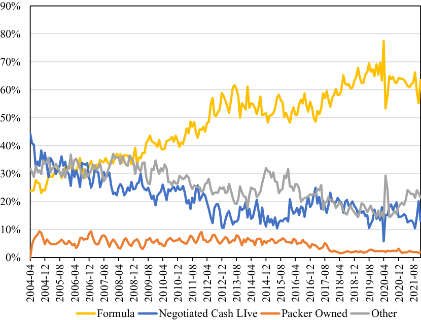
Figure 1. Percent of monthly fed cattle purchases by type, 2004–2021.
Concurrently, the use of formulas as a mechanism for trading live cattle has increased from 25% to between 60% and 70% over this time period. Processing companies have developed strategic alliances with, especially large, feedlot companies so that cattle are slated for delivery to a specific processing company and transaction prices are determined by an agreed-upon formula (Schroeder and Smith, Reference Schroeder and Smith2022). These formulas usually use publicly available negotiated cash sale prices as a base. The development of formula pricing has benefited buyers, sellers, and consumers (Koontz, Reference Koontz2015). Formula contracts often include more complicated pricing structures that compensate sellers based on the quality of individual animals—what is commonly referred to as value-based marketing. Formulas may include, for example, premiums and discounts for meat quality characteristics which are only revealed after animals are processed (e.g., grid pricing based on grades) and thereby incentivize production of higher quality cattle (Schroeder, Coffey, and Tonsor, Reference Schroeder, Coffey and Tonsor2021). Furthermore, formula pricing arrangements help facilitate supply chain management for both buyers and sellers (Schroeder and Smith, Reference Schroeder and Smith2022). For example, Moore (2021) notes that formulas provide market access for many smaller feedlot operations that would likely be bypassed by traditional negotiation processes.
Nonetheless, the decline in the percentage of cattle traded through a negotiated ask-bid process has raised concerns among some market participants (especially cattle producers) that the negotiated cash live cattle market has become too thin (Fischer and Outlaw, Reference Fischer and Outlaw2021). Specifically, questions are being asked as to whether the small percentage of negotiated live cattle transactions (which are used as the base for most formula transactions) lowers the price of formula cattle purchases below that suggested by supply and demand fundamentals. Some market participants have suggested that lower quality cattle are generally purchased through negotiated processes, which lowers the base for remaining higher quality, formula-based live cattle sales. In addition, because live cattle purchases represent the majority of cattle processing costs, concerns have been raised about whether thinning negotiated cash live cattle markets provide an opportunity for price manipulation by processors in an attempt to reduce cattle prices.
In response to these concerns, several Congressional actions are pending that, if implemented, will require that a fixed percentage of cattle be traded using negotiated processes. However, the current reliance on formulas has developed through market processes and reduced overall transaction costs (Koontz, Reference Koontz2015, p. 9). Mandating that minimum percentages of cattle be purchased using negotiated processes represents a substantial market intervention and will add costs to the cattle/beef sector.
We evaluate whether the use of other publicly available cattle or beef prices could be used in formulas as a means for meeting the spirit of proposed Congressional actions. We consider two possibilities: (1) Livestock Mandatory Reporting boxed beef prices and (2) Chicago Mercantile Exchange (CME) live cattle futures prices. Results indicate that live cattle futures prices are reasonable proxies for negotiated cash prices. Consequently, they could be used in addition to, or as a substitute for, directly negotiated prices to meet proposed minimum requirements while providing a less thin base for formula cattle pricing.
2. Literature Review
Recent concerns regarding price transparency and discovery in the fed cattle market are similar to those that have existed for decades (Fischer and Outlaw, Reference Fischer and Outlaw2021). Forty years ago, Ward (Reference Ward1981) noted that cattle producer groups had filed lawsuits that “… allege manipulation of wholesale carcass beef prices to artificially depress spot prices of fed cattle.” (p. 125). In addition, the four-firm steer and heifer packer concentration ratio increased from 36% in 1980 to 78% in 1992 (MacDonald et al., Reference MacDonald, Ollinger, Nelson and Handy2000). These concerns and changes in market structure resulted in a plethora of research regarding the relationships between beef and fed cattle prices as well as thinning markets in the cattle industry (Koontz and Ward, Reference Koontz and Ward2011; Koontz, Reference Koontz2015; Parcell, Reference Parcell2016; Pendell and Schroeder, Reference Pendell and Schroeder2006).
Several proposals have surfaced in recent years with the intent of addressing the thinning live cattle market issue. Senators Tester and Grassley introduced the “50/14” proposal (S.3693) in May 2020, which would have required that 50% of live cattle be procured through a negotiated process with those cattle being slaughtered within 14 days. The stated ambition of S.3693 was “To amend the Agricultural Marketing Act of 1946 to foster efficient markets and increase competition and transparency among packers that purchase livestock from producers.” The U.S. Cattlemen’s Association supported an alternative “30/14” proposal that would require cattle processing facilities to purchase 30% of their live cattle using negotiated cash markets for deliveries occurring within a 14-day period. Around the same time, the National Cattlemen’s Beef Association (NCBA) proposed the “75% Plan,” an ongoing monitoring framework geared towards industry self-regulation, rather than government mandates, as a solution to thinning live cattle cash markets. The NCBA (2020) proposal centered on voluntary packer commitments to procure a specific percentage of live cattle through negotiated processes. The stated goal was to ensure that the regional weekly volume of cattle traded using negotiated processes maintained a level of at least 75% of the “robust price discovery threshold” based on current suggestions proffered by the academic literature for at least 75% of the reporting weeks. However, the NCBA later withdrew their support for this approach and now opposes any legislative or regulatory action that would constrain transactions between cattle feeders and processors.
In September 2020, Senator Fischer introduced the Cattle Market Transparency Act of 2020 that sought to require the USDA to establish regional mandatory minimum thresholds of negotiated cash live cattle transactions and expand the amount of information available through Livestock Mandatory Reporting. A stated goal of the Act was to “…ensure there are a sufficient number of cash transactions to facilitate price discovery… .”Footnote 1 Congress held several hearings on the state of the livestock and beef packing industries in 2021 including the Senate Agriculture Committee on June 23, 2021, the Senate Judiciary Committee on July 28, 2021, and the House Agriculture Committee on July 28, 2021, and October 7, 2021.Footnote 2 These hearings included testimony from various industry stakeholders including cattle producers, cattle industry associations, meat processors, livestock auctions, academic researchers, and industry analysts. In November of 2021, Senators Fischer, Grassley, Tester, and Wyden announced a “compromise cattle market proposal” entitled The Cattle Price Discovery and Transparency Act of 2021 (S.3229).Footnote 3 The Act states that “A packer shall, with respect to a packer processing plant, purchase by negotiated purchase or negotiated grid purchase the percentage of cattle required by the regional mandatory minimum established for the region in which the packer processing plant is located.” The Act gained more than a dozen additional co-sponsors in the Senate and drew attention from the Biden administration.Footnote 4
Presumably, the intent of these proposals is to increase the sample size of negotiated prices so that the base used for formula pricing better reflects the true population mean price (i.e., the price that incorporates all supply and demand fundamentals). If the current negotiated live cattle market does not yield such information, then potential benefits from such actions exist. However, an often-overlooked outcome is that requiring cattle processors to procure a minimum percentage of cattle purchases through direct negotiations necessarily forces feedlot managers to sell the same percentage of cattle using that method. All of these proposals represent market interventions because they require an increase in the percentage of live cattle cash transactions. Currently, cash cattle transactions are used to trade less than 20% of all live cattle (Figure 1). Koontz (Reference Koontz2021) argues that such an approach would add substantial cattle marketing and procurement costs to the cattle/beef sector.
Publicly available commodity price reporting is a classic example of an informational public good that provides value to an economic system (Stigler, Reference Stigler1961). Public goods are both non-rivalrous and non-excludable and are often under-produced by private markets (Mankiw, Reference Mankiw2018). Nonetheless, the availability of price information improves resource allocation and market efficiencies, while reducing asymmetric information bias between buyers and sellers. Several solutions to the underproduction of public goods have been devised. In most cases, however, some type of collective action is required. Such action can be in the form of government legislation or regulation, but trade associations or community groups can also provide the collective action needed to solve public good problems. In some cases, collective action results in the formation of pseudo-markets that nudge outcomes closer to their socially optimal levels (e.g., tradeable fishing quotas, pollution permits, biofuel renewable identification numbers, Johnstone, 2013).
One attempt to provide the public good of cattle pricing is the U.S. Department of Agriculture’s Livestock Mandatory Reporting Act of 1999 (LMR). The purpose of the Act was to establish a process that publicly provides pricing information for cattle, swine, lambs, and meat products traded among private agents. Prior to LMR, a voluntary price reporting system was established by the Agricultural Marketing Act of 1946 (Koontz and Ward, Reference Koontz and Ward2011). The LMR legislation was initially implemented in 2001, lapsed in 2005, and reauthorized in 2015. In March 2022, Congress voted to extend the LMR authorization through September 2022 within the Consolidated Appropriations Act.Footnote 5 The LMR legislation requires participation by all federally inspected cattle processing companies that slaughter at least 125,000 head annually. Although hundreds of smaller plants slaughter cattle (some of them are not federally inspected), the minimum production metric encompasses the plants owned by the largest four packing companies which slaughter the majority of live cattle in the United States. To maintain firm confidentiality, the LMR includes a “3/70/20” guideline. The guideline restricts the provision of aggregated data if (1) there are not at least 3 reporting entities providing data at least 50% of the time over the most recent 60-day time period; (2) any single reporting entity provides more than 70% of the data over the most recent 60-day time period; and (3) a single reporting entity is the sole provider of data for any individual report more than 20% of the time over the most recent 60-day time period. The latter restriction often reduces the number of reported transactions in some regions.
The LMR requires cattle processors to submit live cattle purchase data to the U.S. Department of Agriculture’s Agricultural Marketing Service (AMS) twice daily—at 10:00 a.m. and 2:00 p.m. Eastern Time. Based on these data, AMS posts three different daily live cattle morning summaries as well as an afternoon negotiated price report for each of five major cattle feeding regions. The five regional reports group the major live cattle production states as (1) Colorado, (2) Iowa/Minnesota, (3) Kansas, (4) Nebraska, and (5) Texas/Oklahoma/New Mexico. In addition, the reports delineate price data based on various trading processes. That is, in addition to cattle traded on a live basis, prices are also reported for cattle traded on a dressed basis, quality grids, forward contracts, formulas, and packer ownership.
Koontz and Ward (Reference Koontz and Ward2011) provide a comprehensive review of LMR research. In general, they note that both benefits and costs have occurred relative to the previous voluntary system. Wachenheim and DeVuyst (Reference Wachenheim and DeVuyst2001) discuss the perceived need for mandatory price reporting and note that, prior to LMR, there was a “… widespread, albeit incomplete, agreement that the current system does not provide the necessary level of price transparency…” (p. 180). Koontz (Reference Koontz1999) noted that the voluntary price reporting system was relatively slow to reveal changing market conditions—perhaps because of strategic price reporting.
Pendell and Schroeder (Reference Pendell and Schroeder2006) investigate the impact of LMR on the integration of the five regional fed cattle markets. They find that the markets are highly cointegrated and moved together more closely following the introduction of LMR. More recently, Koontz (Reference Koontz2015) presents a variety of options that could be used to improve problems related to thin live cattle markets. In addition, he notes that the number of weekly LMR price reports was less than that required to obtain a reasonable measure of the population mean during 2014 in some regional markets. Likewise, Parcell (Reference Parcell2016) offers several ideas that could obviate the thin market problems created by the “3/70/20” rule.
Previous research has also considered the lead-lag relationships among live cattle cash prices, live cattle futures prices, and boxed beef prices (Jones et al., Reference Jones, Schroeder, Mintert and Brazle1992; Koontz, Garcia, and Hudson, Reference Koontz, Garcia and Hudson1990; Ward, Reference Ward1981). Using data from the 1960s to 1970s, Kolb and Gay (Reference Kolb and Gay1983) and Oellermann and Farris (Reference Oellermann and Farris1985) found that live cattle futures prices were good predictors of cash cattle prices and important to the price discovery process. More recently, Joseph et al. (2013) found that live cattle futures markets provide the most information for price determination in the fed cattle market. That is, live cattle futures prices lead cash prices, but the reverse is not true. Furthermore, cash cattle prices are solid predictors of boxed beef prices, but boxed beef prices play a minor role in cash cattle price discovery. Schroeder, Tonsor, and Coffey (Reference Schroeder, Tonsor and Coffey2019) note that futures and cash cattle markets are codependent and that information flows between them in both directions.
3. Data
Our research uses LMR live cattle data obtained from the USDA AMS. Price data for negotiated cash transactions for cattle sold live FOB (negotiated cash live) were obtained from report LM_154: National Weekly Direct Slaughter Cattle—Negotiated Purchases. Negotiated cash live prices are reported each Monday and represent a weighted average from transactions that occurred during the preceding week.
Boxed beef prices represent a weighted average of boxed beef cutout values (Livestock Marketing Information Center (LMIC), n.d.). The LMIC collects cutout value data as reported by USDA AMS. Cattle futures prices represent the Friday closing prices for the nearest CME live cattle futures contract for the period 4/16/2004 through 12/31/2021.
The resulting price series represent the week in which live cattle and boxed beef prices are actually reported (as opposed to the week in which the transactions that generated those prices actually occurred). Therefore, week t contains the Monday report for negotiated cash live cattle sold the previous week; Friday boxed beef prices that occur during week t; and the Friday closing price for the nearby live cattle futures contract during week t. The data encompass 925 weeks. During that time period, 30 Friday CME trading holidays occurred. For those weeks, Thursday CME live cattle futures closing prices were used. USDA AMS did not report LMR cash and boxed beef prices during the first three weeks of October 2013 because of a government shutdown. Because closing CME live cattle futures prices (which were reported in October 2013) are highly correlated with live cattle negotiated prices, the weekly percentage changes in futures prices for that month were applied to the live cattle negotiated prices and boxed beef prices to generate proxies for the missing data.
4. Research Approach
Several aspects of thinning negotiated cattle pricing require investigation. First, we evaluate the sample size needed in the negotiated cattle market to obtain a reasonable estimate of the population mean. Second, the data appear to indicate that a structural change among the price relationships may have occurred during the past several years. We quantitatively consider whether such changes have occurred. Third, we evaluate the adequacy of futures market prices and boxed beef prices to serve as proxies for negotiated cash live cattle prices. If either price is found to be a reasonable proxy for cash negotiated prices, then their use as a base for formula-priced cattle could alleviate some concerns regarding the thinning live cattle negotiated market.
4.1. Sample Size
Tomek (Reference Tomek1980) evaluated issues related to thin cattle markets by considering the sample size needed to estimate a population mean when its distribution is unknown. The approach uses Chebyshev’s inequality to produce the following equation:
 $${Pr } \left(\left| \overline{X}-\mu \right| \leq k\right)\geq 1-\left(\sigma ^{2} \over nk^{2}\right)$$
where Pr represents an arbitrary probability; $\overline{X}$
is the sample mean; μ is the unknown population mean; k is an arbitrary acceptable amount of error relative to the population mean; σ 2 is the population variance; and n is the sample size. To implement the equation, the value of
$\overline{X}$
is the sample mean; μ is the unknown population mean; k is an arbitrary acceptable amount of error relative to the population mean; σ 2 is the population variance; and n is the sample size. To implement the equation, the value of $\overline{X}$
is obtained from sample data, and σ 2 is approximated by its sample variance (s 2).
$\overline{X}$
is obtained from sample data, and σ 2 is approximated by its sample variance (s 2).
Solving equation (1) for sample size n results in:
 $$n={s^{2} \over \left(1-Pr\right)k^{2}}\,.$$
Note that the value of n represents the number of observed transactions needed to obtain a representative sample.Footnote 6 A single cattle price transaction usually represents the sale of a pen of cattle with numbers varying from 50 to 250 head. Koontz (Reference Koontz2015) suggests that a pen size of 100 head is representative of the industry. Hence, the number of required transactions calculated in equation (2) is multiplied by 100 for comparison with LMR-reported live cattle numbers. Therefore, equation (2) becomes:
 $$n={s^{2} \over \left(1-Pr\right)k^{2}}\times100\,.$$
Clearly, the value of n in equation (3) is highly sensitive to estimates of the sample variance. The selection of the time period for calculating a weekly sample variance is arbitrary. For example, the variance of weekly live cattle negotiated prices between April 2004 and December 2021 is 467. But, for shorter time periods, the variance is much smaller. Tomek (Reference Tomek1980) used first-differenced weekly prices (over an annual time period) to calculate a sample variance. He notes, “Because the price level need not be rediscovered, a variance based on the first-difference of prices is a sensible measure of the variability of the random variable in question” (p. 438). We use a rolling 26-week time period of first-differenced LMR cash negotiated prices to calculate a weekly price variance because cattle are often fed for a period of 180 days. Consequently, each weekly variance is calculated using the current week’s first-differenced price and those for 25 preceding weeks. After using one week for first-differencing and the next 25 weeks of price data to calculate the variance for the 27th week of the sample, the average of the remaining weekly variances is 6.05 and ranges from 1.25 to 22.59.
Another important element of equation (3) is the value of k. For example, if k is set equal to $1/cwt, equation (3) results in sample sizes in which the actual number of weekly negotiated cattle sales has been large enough to provide a representative sample in all but 9 weeks (1% of the time) between 2004 and 2021. However, if a value for k of $0.50/cwt is used, then the number of head traded through direct negotiations was not large enough to provide a representative sample in 24% of the weeks under consideration. Rather than use an arbitrary value of k, we solve equation (3) as:
 $$k=\sqrt{s^{2}\times 100 \over \left(1-Pr\right)\times n}\,.$$
Using the calculated weekly variances noted above for s 2, the actual weekly number of cattle sold using negotiations for the value of n and an arbitrary value for Pr of 0.95, we calculate a value of k using equation (4) for each week. This approach provides a weekly estimate of k using the revealed preferences of market participants over the past 18 years. The average weekly value of k is calculated to be $0.40/cwt with a range from $0.16/cwt to $1.66/cwt.
Returning to equation (3), we use each weekly value of s 2 and k, along with 0.95 for Pr, to calculate the weekly number of head needed to obtain a 95% probability that the weekly sample size provides a sample mean value that is within ± $0.40/cwt of the true population mean (i.e., representative of the weekly population). The average of these weekly sample sizes is 75,622 head, which represents about 19% of the average weekly number of cattle traded using all methods (391,382). The average weekly number of cattle traded using direct negotiations was 84,571 during the sample. On average, the weekly number of negotiated cattle sales was large enough to result in representative samples.
Nonetheless, substantial weekly variation occurs and is best represented graphically. The use of weekly data, however, renders a graphical representation that is visually incomprehensible. Therefore, the weekly sample sizes calculated using equation (3) were averaged within each month for illustrative purposes. Figure 2 shows the number of cattle sold using direct negotiations and the sample size needed to provide a representative sample (using k = 0.40 and Pr = 0.95). The number of cattle sold using direct negotiations was often smaller than the suggested sample size needed to obtain a representative sample. Given that the values of k and Pr are constants for each week in equation (3), variations in weekly representative sample sizes are the result of changes in weekly price variances. The results from equation (3) indicate that negotiated weekly cattle trades were not large enough to provide a representative sample 38% of the time since 2004 (and 70% of the time since 2014). Koontz (Reference Koontz2015) notes that the number of cattle sold through direct negotiations was often less than needed to obtain a representative sample at various times, but especially during 2014. Our updated sample indicates that this continued throughout most of 2015 through 2017. More recently, lower weekly price variation has reduced the required sample size so that the number of cattle sold through negotiations has been sufficient in most weeks based on our parameters. The exception has been increased price variation during 2020 caused by the COVID-19 pandemic and its associated market disruptions.
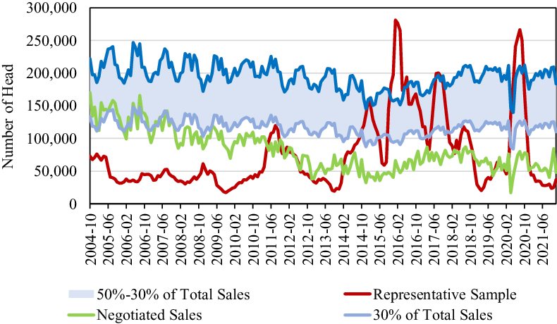
Figure 2. Monthly averages of weekly representative sample sizes, negotiated cattle sales, 30% of total cattle sales, and 50% of total cattle sales, 2004–2021.
In addition to the weekly representative sample size calculations and the actual number of head traded using direct negotiations, Figure 2 also presents the number of head that would have been traded using direct negotiations on a weekly basis (again, weekly averages within each month for ease of illustration) for two proposals—the U.S. Cattlemen’s Association’s suggested 30% rule and S.3693’s mandate of 50%. Because these fixed percentages are independent of price variation, the actual sample sizes were not large enough to provide representative samples in several weeks.Footnote 7 On the other hand, the 30% proposal provides a weekly sample size that is larger than needed 81% of the time (59% of the time since 2014). The 50% proposal provides a sample that is larger than needed 92% of the time (84% of the time since 2014). Given that the costs of any fixed rule will be borne by participants across the cattle/beef industry, sample sizes should be no larger than needed to be representative of weekly populations to minimize the costs of market intervention.
The sample size calculations noted above assume that no differences exist among the quality of cattle sold using the various methods and also do not account for the potential regional differences that are the focus of S.3229. The robust weekly negotiated trade numbers suggested by the NCBA (2020) are as follows: Texas/Oklahoma/New Mexico, 13,000 head; Kansas, 21,000 head; Nebraska/Colorado, 36,000 head; and Iowa/Minnesota, 16,000 head. The total of these regional values is 86,000 head, which is similar to the average weekly sample size (75,622 head) obtained from equation (3). Nonetheless, any fixed percentage rule abstracts from changes in price variability over time.
Table 1 shows that, relative to the 2004–2015 period, the Texas/Oklahoma/New Mexico region’s weekly number of cattle that were negotiated on a live basis declined substantially after 2015. Kansas and Colorado experienced moderate declines, while Nebraska experienced a negligible increase. Since 2015, the Colorado reporting region had 125 weeks in which no data are reported because of confidentiality reasons. Given that the Texas/Oklahoma/New Mexico region accounts for an average of 20–25% of cattle feeding annually, the reduction in live cash negotiations in this region is a primary concern regarding thin cattle markets (USDA NASS, n.d.b).
Table 1. Regional average weekly negotiated cash and total live cattle sales

a The LMR reports add Missouri to the Minnesota/Iowa region for these data.
b The average total weekly steer and heifer slaughter values were calculated for each state using the U.S. monthly percentage of steer and heifers slaughtered relative to total slaughter (USDA NASS, n.d.a). This percentage was applied to the monthly total cattle slaughter for each state (USDA Livestock Slaughter, annual summaries). The state values were then aggregated to the defined LMR regions, and weekly averages were obtained for each month and then averaged for each of the indicated time periods. The Minnesota/Iowa/Missouri region values could not be calculated because disclosure rules prevent the data from being published.
4.2. Price Relationships
Figure 3 presents monthly averages of weekly LMR negotiated cash live prices, cattle futures prices, and boxed beef prices. Clearly, negotiated live cattle prices closely follow CME cattle futures prices as the two data series are almost indistinguishable on a monthly basis. It appears that until recently, boxed beef prices followed a pattern similar to negotiated cash live cattle prices.
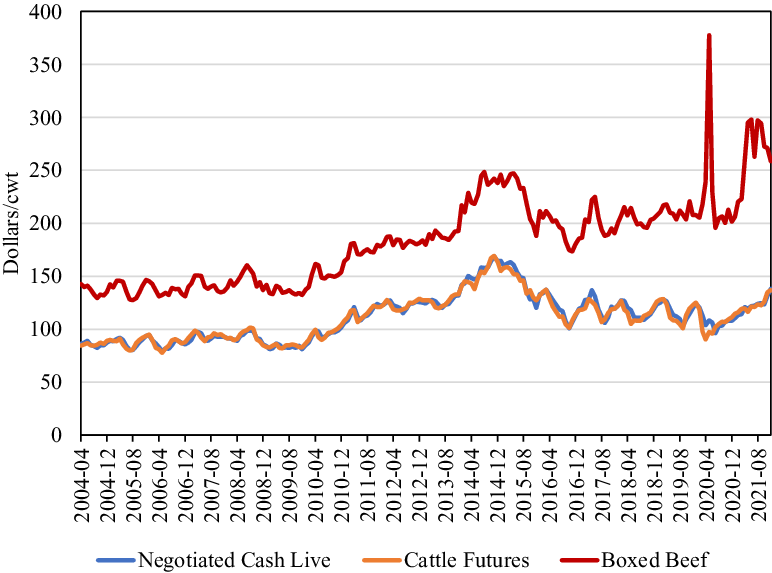
Figure 3. Monthly average negotiated cash live, cattle futures, and boxed beef prices, 2004–2021.
Table 2 presents the simple correlation coefficients for the three weekly price series: LMR-reported negotiated live cattle prices; Friday (or Thursday in the case of Friday holidays) closing values of nearby live cattle futures prices; and LMR-reported boxed beef prices. For the entire April 2004–December 2021 sample, cash prices are highly correlated with nearby futures prices (0.976) but much less so with boxed beef prices (0.774). Similarly, nearby futures prices and boxed beef prices have a correlation coefficient of 0.735.
Table 2. Weekly cash cattle, live cattle futures, and boxed beef price correlations

Figure 4 indicates that the difference between live cattle futures prices and negotiated live cattle prices (on a monthly basis) has generally varied around zero. However, the difference between boxed beef prices and negotiated live cattle prices has clearly trended upward over the past 14 years and, even more so, since the middle of the past decade. Thus, it may be that structural changes have occurred in the pricing system.
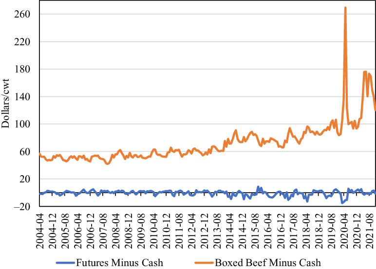
Figure 4. Difference between futures and boxed beef and cash prices, 2004–2021.
4.3. Structural Change Tests
We use an empirical fluctuation process (EFP) to test for a structural change in the relationship between negotiated cash live prices and both boxed beef and live cattle futures price. The EFP function from the R package “strucchange” computes optimal breakpoints based on recursive OLS estimates of the model regression coefficients (Zeileis et al., Reference Zeileis, Leisch, Hornik and Kleiber2002). Weekly average cattle prices tend to follow seasonal patterns so that we might expect structural changes in price relationships to occur over the course of a year rather than in any single week. Therefore, the EFP test was used to provide general guidance on the likelihood and time frame of structural change rather than to identify exact breakpoints (Zeileis et al., Reference Zeileis, Kleiber, Krämer and Hornik2003). A bandwidth test parameter of 0.2 was chosen to specify a minimum allowable structural segment length of one-fifth of the total data series.
Using these parameters, the EFP recursive test for negotiated cash and boxed beef prices (t-2) strongly suggests a single breakpoint using data from two different time periods: (1) a “pre-COVID” period from 2004 to 2019, and (2) the full period from 2004 to 2021. In both cases, the Bayesian Information Criterion (BIC) decreased by more than 10% for a single breakpoint relative to a no-breakpoint model. The EFP test estimated the single breakpoint to fall in June 2016 using pre-COVID data, and in June 2017 using data for the entire period. Models that included more than one breakpoint produced no substantial improvement (less than a 2% decrease) in the BIC for either time period. Similar tests conducted for negotiated cash and live cattle futures prices showed no significant evidence of structural change, producing less than a 3% overall decrease in BIC for any non-zero number of breakpoints. Results of the structural change tests were combined with other available information, including visual inspection of the three price series (Figure 3), price correlations (Table 2), and knowledge of events affecting the cattle industry during this time period.Footnote 8 After assessing these factors, our subsequent empirical analyses include a binary variable that represents a structural change in the market starting in 2016.
Table 2 presents simple price correlations for two subsamples based on the structural change tests. For the 2004–2015 subsample, all three correlation coefficients are equal to or greater than 0.975. For the 2016–2021 subsample, cash prices continue to be relatively highly correlated with futures prices (0.832). However, cash prices are much less correlated with boxed beef prices (0.214) during this period. And, futures prices are even less correlated with boxed beef prices (0.108). Consequently, the structural shift between boxed beef prices and both cash and futures prices noted above appears to be manifested in much lower price correlation coefficients since 2016.
4.4. Regression Models
The goal of our regression models is to find a metric that is a good predictor of live cattle negotiated prices. We investigate the potential for using LMR boxed beef price data as a proxy for LMR cash negotiated live cattle prices by estimating the following equation:
 $$\textit{PLIVE}_{t}=\alpha _{0}+\beta _{i} PBOX_{t-i}+\gamma _{1}D_{16}+\varepsilon _{t}$$
where PLIVEt is the weekly LMR cash negotiated live cattle price in week t; PBOX t − i is the weekly LMR price of boxed beef in i weeks preceding live cattle prices reported in week t; D 16 is a binary variable that represents the indicated structural change beginning in week 1 of 2016; ϵ t is an error term which may have autoregressive properties; and α 0, β i , and γ 1 are parameters to be estimated. It is important to note that LMR negotiated live cash cattle prices are reported on Monday of each week. However, the data used to produce the report are collected from the preceding week. Therefore, the lag length on the PBOX variable cannot begin later than week t-1 as it is that week’s price which is actually reported in the following week. Other longer lag lengths may better fit the data and will be investigated below.
To evaluate the potential for using CME Live Cattle Futures prices as a proxy for LMR cash negotiated live cattle prices, we estimate the following equation:
 $$\textit{PLIVE}_{t}=\alpha _{0}+\beta _{i} PFUT_{t-i}+\gamma _{1}D_{16}+\varepsilon _{t}$$
where PFUT t − i is the Friday (or Thursday in the case of Friday holidays) closing value of the nearby CME live cattle futures contract for i weeks preceding the live cattle price report in week t. Again, it is important to note that the price of live LMR negotiated cash cattle are reported on Monday of each week, and the data used to produce the report are collected during the preceding week. Therefore, the lag length on PFUT cannot begin later than week t-2, since the value of PFUT in time period t has not yet occurred. In addition, live cattle prices collected in week t-1 (but reported in week t) could not include information from PFUT in time period t-1 because we use Friday closing prices. Other longer lag lengths may better fit the data and will be investigated below.
5. Empirical Results
Based on Augmented Dickey-Fuller and Phillips-Perron unit root tests, the boxed beef price series is stationary, but the cash live cattle and futures market price data are not.Footnote 9 Because the cash live cattle price series is used as the dependent variable in equations (5) and (6), we test whether the data are cointegrated by considering the regression residuals in each model. We reject the null hypothesis of non-stationarity in both sets of residuals with p-values much smaller than 0.05. Hence, the regression equations represent cointegrating vectors, and we conclude that the regression results are not spurious.
Table 3 presents generalized least squares coefficient estimates for equation (5). Several lag lengths on boxed beef price were considered, but a lag of two weeks provided the best fit of the data. Finally, the Durbin-Watson statistic indicated the presence of autocorrelation. Hence, a first-order autocorrelation parameter was included in the regression, and robust standard errors were calculated for all coefficient estimates using the vcovHAC function in the R package “sandwich” (Zeileis, Reference Zeileis2004). The t-statistics for the coefficient estimates reported in Table 3 were computed using a heteroscedastic- and autocorrelation-consistent (HAC) covariance matrix. The estimated coefficient on boxed beef prices lagged two periods is highly significant and positive. The binary variable and the autoregressive error coefficient are both highly significant.
Table 3. Regression results

Notes: t-values are in parentheses.
The last column in Table 3 presents generalized least squares regression results of equation (6). The model with the best fit included futures prices lagged two weeks and the binary intercept shift variable. The futures price coefficient is positive and highly significant (with a standard error of 0.0159) as is the binary coefficient estimate. Note that the estimated coefficient on the lagged (t-2) futures market price is equal to 1.01. A t-test of the null hypothesis that the estimate of 1.01 is statistically different from 1.0 is clearly rejected (a t-value of 0.63). Hence, on a weekly basis, a $1/cwt change in live cattle futures price lagged by two weeks corresponds to a statistically identical change to contemporaneous negotiated live cattle cash prices. Consequently, live cattle futures prices are a solid proxy for the latter.
Based on the adjusted R-squared statistics, the live cattle futures model fits the data much better than the boxed beef model. Consequently, the root mean squared error of the live cattle futures model (3.2% of the mean of the dependent variable) is much smaller than the root mean squared error of the boxed beef model (11.3%). Hence, nearby live cattle futures prices lagged two weeks do a better job of predicting live cash prices than boxed beef prices lagged 2 weeks.
As noted above, the percentage of cattle traded via negotiated cash sales over the past several years has been relatively small. This raises concerns as to the usefulness of the regression models. That is, if the negotiated cash prices of the past few years are not representative of the population, then the value of the live cattle futures (or boxed beef) prices may be in question. The growing concerns about the negotiated cattle market becoming too thin seem to have risen as the percentage of cattle traded in this manner declined below 20%. It appears that industry participants did not believe the negotiated cash market was too thin as long as the percentage of these trades exceeded this level. In general, the percentage of cattle trade via cash negotiations declined below 20% during 2012 (and continues today). Therefore, we also estimated the previously described live cattle futures model using only data for 2004 through 2011. The regression results are almost identical to those reported in Table 3.Footnote 10
6. Conclusions
Some cattle producers and producer organizations have raised concerns regarding the methods used by beef processors to secure live cattle supplies. While packer ownership of live cattle has declined over the past few years, the percentage of live cattle procured through formula pricing has increased markedly. Consequently, the percentage of live cattle procured through traditional negotiations has declined from 35 to 40% 15 years ago to less than 20% today. In some weeks, however, the percentage is even lower. Furthermore, the historical trend raises concern about the ability of future negotiated cattle prices to represent supply and demand fundamentals along with concerns about potential price manipulation. Most formula pricing of cattle involves strategic alliances between feedlots and processors. In addition, publicly reported live cattle negotiated prices provide a base for many formula pricing agreements. If the negotiated cash market has become too thin, then supply and demand beef industry fundamentals may not be adequately reflected in the cattle market.
Several proposals have been offered to reduce the thinness of the live cattle market. Most mandate that a fixed percentage of cattle be traded each week through direct negotiations. Regardless of the selected fixed percentage, however, each represents an intervention between sellers and buyers of live cattle. Furthermore, the sample size needed to reasonably represent the population mean differs each week depending upon the variability of prices. Price variability is not considered by any of the proposed fixed percentage rules. Sellers and buyers have gravitated towards formula pricing because of cost advantages for both groups. An intervention in this market would, therefore, add costs to the beef production system, which harms beef consumers, cattle processors, and cattle producers.
Rather than legislating that a fixed percentage of live cattle must be traded using only direct negotiations, we propose allowing pricing methods and formulas that use a proxy for live cattle prices to be counted towards this fixed percentage. We find that live cattle futures prices have historically provided a close proxy to negotiated live cattle prices. In addition, live cattle futures prices are publicly available at a very low cost and result from hundreds of market participants incorporating information regarding supply and demand fundamentals. Of course, concerns regarding futures market price variability and convergence as contracts near expiration dates are well-founded. Nonetheless, our sample uses price data encompassing these situations. One could use the next nearby live cattle contract if nearness to an expiration date is a concern.
The concerns about the use of thinly traded negotiated prices in formula pricing contracts can be somewhat alleviated by using futures prices as the base for formula-priced cattle. This approach would allow the price of a liquid, actively traded market that has a low risk of price manipulation to be used as the base for formula prices. One would want such markets to be a reasonable reflection of supply and demand conditions. Our quantitative analyses show this to be the case. Consequently, allowing the use of formula transactions based on live cattle futures to contribute to proposed fixed percentages of negotiated cattle purchases would reduce the cost of proposed market interventions. The approach proposed in this paper allows market participants to retain their ability to use and benefit from formula pricing.
Industry participants who support a fixed percentage cash mandate have expressed concerns that formula prices are based on a negotiated cash market that is considered by many to be too thin. They surmise that, because only a few buyers are involved in the thin market, the potential exists for the manipulation of cash cattle prices. We have shown that live cattle futures prices can serve as a good proxy and potential substitute for cash live cattle prices as a base in formulas. In contrast to negotiated cash cattle prices reported through LMR, live cattle futures are traded in an independent futures exchange that is accessible to a much wider range of market participants and where current prices are reported almost instantly. Nonetheless, a further reduction in the use of cash live cattle trade could potentially alter the relationship between cattle futures prices and cash prices. A counterbalance to this problem, however, is that live cattle can be delivered as a means of settling futures contracts. Hence, the cash market is implicitly tied to the futures market even if the cash market thins further.
Finally, our proposed policy addendum does not improve price discovery in the cattle market. Such an improvement would likely require details regarding formula price contracts to be revealed, which would raise issues of confidentiality.Footnote 11 Nonetheless, allowing formula transactions based on either futures or boxed beef prices to count towards a minimum cash negotiation percentage does improve price transparency. That is, reductions in market uncertainty and the amelioration of concerns regarding price manipulation in thin markets bolster confidence in the market system. In addition, the use of futures prices facilitates a more direct hedging opportunity for cattle producers with respect to formula-priced cattle. If a fixed percentage of live cattle must be traded using negotiated live prices, we propose that formulas using live cattle futures prices as a base be allowed to meet this fixed percentage. In this way, cattle producers and processors have the option of using a less restrictive approach to trading live cattle while retaining the benefits of formula pricing.
Author Contributions
Conceptualization—G.W.B., K.S., B.C.
Methodology—G.W.B., K.S., B.C.
Formal Analysis—G.W.B., K.S., B.C.
Data Curation—G.W.B., K.S., B.C.
Writing-Original Draft—G.W.B.
Writing-Review and Editing—G.W.B., K.S., B.C.
Supervision—G.W.B.
Funding Acquisition—not applicable.
Financial Support
This research received no specific grant from any funding agency, commercial, or not-for-profit sectors.
Disclosures
The authors have no conflicts of interest to declare.


 Open access