


1. Introduction
Past research on the retail beef market has focused extensively on intrinsic attributes of meat, such as fat content or marbling, tenderness, and taste (Feuz et al., Reference Feuz, Umberger, Calkins and Sitz2004; Lusk and Parker, Reference Lusk and Parker2009; Lusk et al., Reference Lusk, Fox, Schroeder, Mintert and Koohmaraie2001; O’Quinn et al., Reference O’Quinn, Woerner, Engle, Chapman, Legako, Brooks, Belk and Tatum2016; Vierck et al., Reference Vierck, Gonzalez, Houser, Boyle and O’Quinn2019). Numerous studies have examined less tangible attributes such as geographic origin of production and traceability (Adalja et al., Reference Adalja, Hanson, Towe and Tselepidakis2015; Dobbs et al., Reference Dobbs, Jensen, Leffew, English, Lambert and Clark2016; Loureiro and Umberger, Reference Loureiro and Umberger2003); method of production such as conventional versus organic, grass feed, hormone free, and GM free (Evans, et al. Reference Evans, D’Souza, Collins, Brown and Sperow2011; Tonsor et al. Reference Tonsor, Schroeder, Fox and Biere2005); and additional labeling preferences indicating qualities such as safety (Lim et al., Reference Lim, Hu, Maynard and Goddard2013).
Among these attributes, meat color can influence consumer decisions. Pohlman et al. (Reference Pohlman, Pohlman, Anthony and Yang2019) demonstrated that consumers make quality inferences based in part on meat color, and a visual appraisal of beef, based primarily on color, is often more important to consumers than price. Research has shown the preferred color of beef is a bright cherry red (Carpenter, Cornforth, and Whittier, Reference Carpenter, Cornforth and Whittier2001; Killinger et al., Reference Killinger, Calkins, Umberger, Feuz and Eskridge2004; Ramanathan and Mancini, Reference Ramanathan and Mancini2018). Through prolonged exposure to oxygen, retail beef begins to discolor, turning brownish red to brown. Consumers often perceive this discoloration as a condition of “unwholesomeness” (Faustman and Cassens, Reference Faustman and Cassens1989), which decreases their willingness to pay (WTP) for the discolored beef (Feuz, Norwood, and Ramanathan, Reference Feuz, Norwood and Ramanathan2019; Grebitus et al., Reference Grebitus, Jensen, Roosen and Sebranek2013; Grebitus, Jensen, and Roosen, Reference Grebitus, Jensen and Roosen2013). As a result, beef cuts are marked down in price, faced and repackaged, ground, or discarded (Smith et al., Reference Smith, Morgan, Sofos and Tatum1996; Suman et al., Reference Suman, Hunt, Nair and Rentfrow2014). It is unknown which of these options is used most prevalantly by retailers. It is, however, common to find discolored beef cuts routinely marked down for quick sale at many grocery outlets. Retailers recognize that consumers have a lower WTP for discolored beef yet hope to minimize revenue loss by marking down the price rather than simply discarding.
Perhaps this marketing decision has been oversimplified. Discolored beef marked down in price and sold provides additional revenue that would otherwise be lost if the meat were discarded. However, what effect does marketing this discolored beef alongside nondiscolored (bright, cherry red) beef have on the value of the nondiscolored beef? Is there a spillover effect, whereby the presence of a discolored steak alters the perceived quality or value of nondiscolored steaks? It is conceivable that the spillover effect is negative, meaning the value of the nondiscolored steak falls because of the presence of a nearby discolored steak. If consumers perceive that poor meat management practices cause the discoloration, they might believe that those poor practices threaten the safety of all the meat in the store.
Conversely, the presence of a discolored steak might raise the perceived quality of the nondiscolored steak by making it seem more appealing by comparison. This would be a positive spillover effect. Another possibility would be that marketing discolored steaks alongside nondiscolored steaks may have no effect on consumer preferences for the nondiscolored steaks. Perhaps different subsets of consumers display all three reactions, with some liking the nondiscolored steak more, some less, and some the same. This research measures the direction and size of the spillover effect for consumers overall and for subsets of consumers.
We achieve this objective using two sets of data. One comes from an Internet survey of Americans (referred to as Study 1) in which respondents were asked directly how the presence of a discolored steak alters their perception of a nondiscolored steak. They were also asked an open-ended question regarding their perception on what causes discoloration, because this could influence the direction of the spillover effect. The second set of data comes from a controlled experiment (Study 2) in which subjects viewed three steaks in a choice set and rated the appeal of the most and least appealing steaks. By randomly varying whether a discolored steak is present in the choice sets, we are able to measure the spillover effect.
1.1. Literature on spillover effects
Although some economic models might explain the value of a good solely in terms of its own attributes, a wealth of studies have demonstrated how the attributes of dissimilar goods in a choice set can influence one another’s values. The marketing literature has devoted considerable resources to studying the “decoy” effect, also referred to as an “attraction” effect, whereby the addition of a third option alters a consumer’s preference for the two original items (Heath and Chatterjee, Reference Heath and Chatterjee1995; Sellers-Rubio and Nacolau-Gonzalbez, Reference Sellers-Rubio and Nacolau-Gonzalbez2015). Specifically, suppose there are two items, A and B. Some consumers prefer A, and some consumers prefer B. If a third product, C, is added that is dominated by A but not B across all attributes (e.g., both in terms of price and quality), then consumers will increase purchases of A. Likewise, if C is dominated by B but not A, then its presence will increase purchases of B.
To illustrate, suppose there are originally two steaks for sale, one of higher quality (rib eye) but also a higher price per pound and the other of lower quality (sirloin) and at a lower price per pound. If a discolored rib eye is added to the choice set at the same price as the nondiscolored rib eye, its presence could increase sales of the nondiscolored rib eye.
Other studies have documented a “compromise” effect: Consumers increase their perception of the value of an item if it is depicted as a moderate option rather than an extreme option (Levav, Kivetz, and Cho, Reference Levav, Kivetz and Cho2010). In this case, consumers might state their WTP for a low-quality sirloin steak as $5.00/lb. but then increase this WTP when a discolored sirloin steak is added to the choice set. Although the steak originally seemed “low” quality, the presence of the discolored steak now makes it seem a more “moderate” quality, thereby increasing its value to consumers.
Both the attraction and compromise effects are more likely to occur when consumers are less familiar with the good and its attributes (Levav, Kivetz, and Cho, Reference Levav, Kivetz and Cho2010). The extent to which the attributes are meaningful also influences decoy effects. If steak grades like Select, Choice, and Prime are less meaningful to consumers, they are more likely to exhibit the decoy effect (Ratneshwar, Shocker, and Steward, Reference Ratneshwar, Shocker and Steward1987), though this might be defined by some researchers as less familiarity.
The value of a good can be dependent on other goods in a choice set in cases where consumers exhibit bounded rationality and must employ cognitive effort and heuristics to arrive at a choice. That is, consumers are not just choosing the good that they most prefer, they are actively trying to decide which one they prefer the most from a choice set, and they make this decision based partly on environmental cues. The presence of a discolored steak in a choice set might provide cues the individual uses to infer the quality of other nondiscolored steaks. If a person associates discoloration with poor management, he or she might infer that the nondiscolored steaks, though appearing safe to eat, have also been managed poorly and could thus pose safety hazards. This would cause the person to reduce the value he or she places on nondiscolored steaks in the presence of discolored steaks.
There is reasonable evidence to suggest that the presence of discolored steaks affects the value consumers place on nondiscolored steaks. The preceding paragraph suggests that a discolored steak reduces the value of its nondiscolored neighbors, whereas the decoy and compromise effects suggest the opposite. Alternatively, the effects could offset one another such that a discolored steak has no impact on surrounding nondiscolored steaks. Determining the direction and magnitude of the spillover effect of marketing discolored beef together with nondiscolored beef can provide evidence for which of these marketing phenomena, if any, occurs in this situation.
2. Methods and data
2.1. Study 1
Is there a spillover effect, whereby the presence of a discolored steak makes nondiscolored steaks more or less appealing? One way of answering this simply is to pose the question to consumers through a survey. In fall 2017, we administered an Internet survey to a sample of 2,598 U.S. respondents acquired by Survey Sampling International using Qualtrics software. The sample was intended to be representative of all U.S. consumers, and the sample demographics generally fit the desired population reasonably well.Footnote 1
Among the questions asked was one concerning the spillover effect. Subjects were shown a picture of two steaks—one discolored and the other nondiscolored—and were explicitly asked how the discolored steak affected their perception of the quality of the nondiscolored steak. Figure 1 illustrates the question as asked in the survey (question order was randomized across respondents). By analyzing how responses to the two questions differ across respondents, we can begin to understand potential spillover effects.
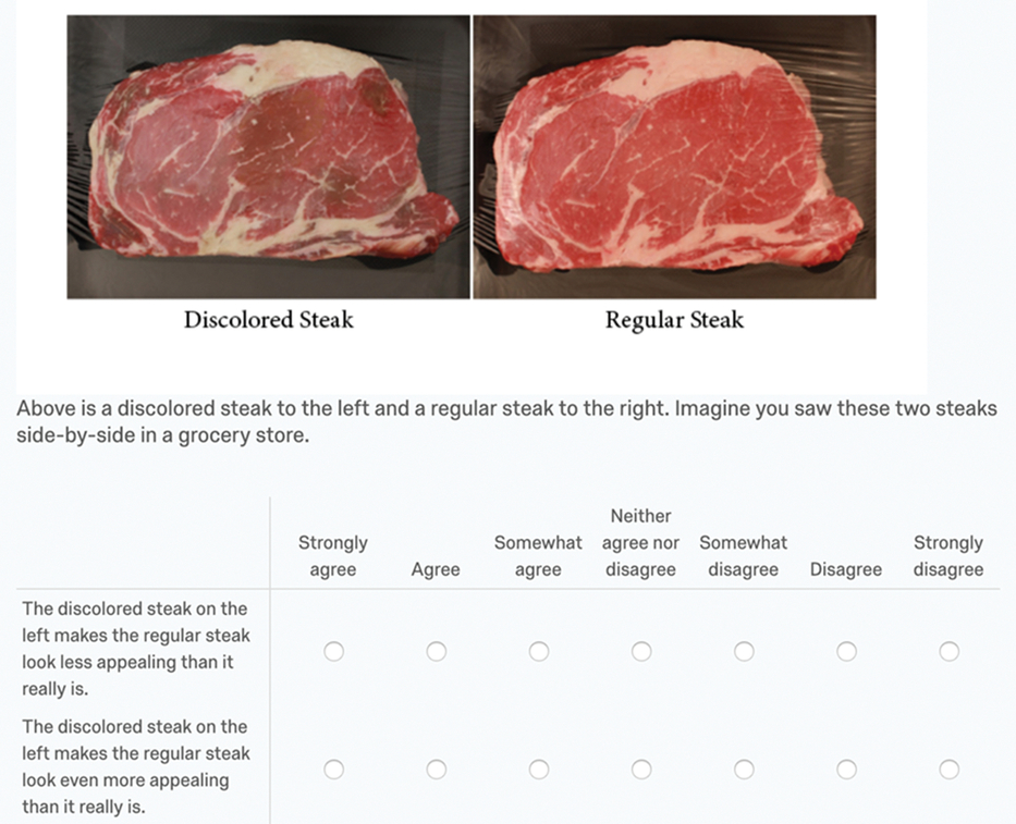
Figure 1. Grid-style question from nationwide consumer survey.
The survey also posed an open-ended question: “What do you believe causes discoloration in raw beef? Please answer in your own words using at least one sentence.” By analyzing the content of the answers, we can assess whether people believe discoloration to be caused by a factor that could affect all other beef products or by a factor unique to each individual beef item, thereby allowing us to determine whether the reasons for discoloration should suggest the presence of a spillover effect. Additionally, respondents were asked what they do with discolored meat at home and whether they believe grocery stores should sell discolored meat, which aids us in understanding whether discoloration is seen as a systemic management problem that would affect the value of all meat sold in the store.
2.2. Study 2
The second study consisted of a controlled in-person experiment in which subjects were asked to rate the appeal of a set of steaks, with some participant choice sets containing a discolored steak and others containing only nondiscolored steaks. The experiment was conducted on March 12, 2018, at the Robert M. Kerr Food and Agricultural Products Center on the Oklahoma State University campus. In total, 118 people participated in the experiment, though 1 subject did not complete the entire questionnaire, resulting in 117 observations. Subjects were recruited by sending out e-mail invitations to the Division of Agricultural Sciences and Natural Resources at Oklahoma State University. Additionally, a sign was placed on the sidewalk adjacent to the building where the experiment was held, inviting people to participate. Key demographic variables of participants were collected and compared with the U.S. population demographics. Table A2 in the Appendix summarizes the sample demographics. Additional discussion on how well the survey sample fit the targeted demographics is also included in the Appendix.
Three Choice rib-eye steaks, approximately 3.5-inches thick, were purchased from a local meat purveyor. Four days before the experiment was held, the steaks were cut horizontally through the center to yield six steaks to be used in the experiment. By cutting the steaks in this fashion, each steak could be paired with a nearly identical or mirror-image counterpart steak, reducing variability between the steaks and helping to eliminate confounding variables in the experiment. Three of the nonpaired steaks were promptly vacuum-sealed and placed in a dark cooler until the day of the experiment. The other three steaks were placed on foam trays with absorbent pads and wrapped with PVC film (oxygen-permeable polyvinyl chloride fresh meat film). After packaging, the steaks were placed in a coffin-style open display case maintained at 2°C ± 1 under continuous lighting for 4 days. During these 4 days, the steaks became increasingly discolored, as would naturally occur in a retail display when approaching the “sell-by” date. For additional information about the level of discoloration of these steaks and how discoloration was measured, see Table A3 in the Appendix.
On the day of the experiment, approximately 30 minutes before participants arrived (just long enough for the fresh beef to bloom and assume a bright cherry-red color) the vacuum-sealed steaks were removed from the dark cooler and packaged in the same way as the discolored steaks. We then had three nondiscolored and three discolored steaks to be used in the treatments.
There were two treatments for the experiment, with approximately half of the participants randomly receiving each treatment. In the discolored treatment, three steaks were presented in the retail-style cooler, just as they would be found at a retail store ready for purchase. Two participants at a time were escorted to the retail cooler. Two of the steaks presented were nondiscolored steaks, whereas the other was discolored; all three were randomly chosen and varied for each set of two participants. In the nondiscolored treatment, all three steaks were nondiscolored. Subjects were randomly assigned to the discolored/nondiscolored treatments by regularly rotating the treatments throughout the experiment. The order in which the steaks were displayed was also randomized.
Each participant was initially given “Survey Sheet 1” to complete (see Figure A1 in the Appendix for an example of the survey sheet). At the top of the first page, participants were instructed to first carefully observe the three steaks in front of them. Then they were asked to determine which steak they liked the most/least (randomly assigned to consider most or least) and, with their chosen steak in mind, indicate the extent to which they agreed or disagreed with the statements that followed. The questionnaire did not actually ask subjects to indicate which steaks were their most and least favorite but rather to make their selections in their own minds and respond to the statements about their selection. We assume (because all steaks were virtually identical except for color) that a discolored steak was never the most favored steak. The second page of “Survey Sheet 1” was identical to the first, except that participants were instructed to respond to the statements while considering the opposite choice, most or least liked steak. The 12 statements (6 statements times two sets of questions) on “Survey Sheet 1” are as follows:
1. The quality of this rib-eye steak is high.
2. I would seriously consider purchasing this steak.
3. If offered at a reasonable price, people would purchase this steak.
4. Most people would like the taste of this steak.
5. I would purchase this steak for ($X) per pound. (X varied randomly by $0.25 increments from $5.00 to $15.00.)
6. I would purchase this steak for ($X) per pound. (X varied randomly by $0.25 increments from $5.00 to $15.00.)
Each of the statements was followed by a 7-point Likert scale of agreement options (from 1 = strongly disagree to 7 = strongly agree).
After completing “Survey Sheet 1,” the two participants were escorted away from the retail cooler and given “Survey Sheet 2” to complete, which collected the demographic information summarized in Table A2 (see Appendix). Upon completion of “Survey Sheet 2,” participants were given $10 in appreciation for their participation. Table 1 summarizes the responses to the statements for both the most and least liked steaks.
Table 1. Summary of responses to questionnaire statements
a Price per pound varied randomly by $0.25 increments from $5.00 to $15.00.
The questionnaire results are analyzed as follows: First, we performed a factor analysis on all six statements to discern the number of latent factors that might influence response patterns (see Table A4 in the Appendix). This analysis is needed to determine the most appropriate methodology for analyzing the data. Although the factor analysis finds that a single factor explains responses to all statements (suggesting that the responses to the Likert scales for all six statements can be summed to create one variable denoting steak desirability), we chose to aggregate statements 1–4 and statements 5 and 6 separately for analysis. We do this for three reasons: First, the sizes of the factor loadings differ between these sets of statements. Second, the statements are different in nature. Third, by analyzing the combined statements 5 and 6 separately, we can estimate WTP for each steak type (most vs. least preferred).
The objective of Study 2 is to determine how the presence of a discolored steak influences the appeal and value of the nondiscolored steak. We analyze the response patterns to statements 1–4 by first summing the scores and then analyzing how this sum changes when a discolored steak is included in a choice set using a finite mixture regression model (FMM). The scores can be summed to create one variable because there is only one latent factor influencing their value. The model can be represented as
 $${S_{i,c}} = {\alpha _{0,c}} + {\alpha _{1,c}}\left( {{D_i}} \right) + {X_i}{\beta _c} + {e_{i,c}},$$
where Si,c is the sum of the response to statements 1–4 for participants’ most liked steak; Di is an indicator variable that equals 1 if a discolored steak is present and 0 otherwise; Xi is a vector of demographic variables; ei,c is an error term; and α 0,c, α 1,c, and β c are parameters to be estimated. Subscript c refers to classes of individuals. If a regular regression is used, then all individuals belong to one class, c = 1, and all respondents share the same parameter estimates. However, an FMM allows for two classes, c = 1 or 2, each of which possesses its own distinct parameter estimates.Footnote 2
The spillover effect depends on the value and statistical significance of the α 1,c parameter. If positive, individuals in this class find the nondiscolored steak more appealing in the presence of a discolored steak. If negative, the opposite is true. If α 1,c is not statistically significant, then the presence of a discolored steak does not influence the appeal of the nondiscolored steak. We use the FMM to capture heterogeneity in the spillover effect. For example, the first-class respondents might be associated with a positive spillover effect, α 1,1 > 0, whereas the second-class demonstrates a negative spillover effect, α 1,2 < 0.
Statements 5 and 6 concern respondents’ willingness to purchase the steak at a stated price, and variations in their answers in response to price variations allow us to calculate their maximum WTP for the chosen steak by using an ordered logit model. The responses to these two statements are assumed to be generated from the random utility model, specified as
 $${U_{i,c}} = {\alpha _{1,c}}\left( {{D_i}} \right) - {\gamma _c}\left( {{P_i}} \right) + {X_i}{\beta _c} + {e_{i,c}},$$
where U i,c is the latent utility generated from being able to purchase the best steak at price P i; α 1,c, γ c, and β c are parameters to be estimated; and the other variables are as previously defined in equation (1). Intercepts are not needed in the model because they are implicitly reflected in the threshold parameters. An ordered logit model allows us to estimate the parameters in equation (2). The change in the value of the nondiscolored steak in the presence of the discolored steak is then calculated as
 $$WT{P_c} = {{{\alpha _{1,c}}} \over { - {\gamma _c}}}.$$
If α 1,c is positive, then consumers are willing to pay more for the nondiscolored steak when a discolored steak is present; if negative, then they will pay less. If α 1,c is not statistically significant, then the steak’s value is unchanged. As before, subscript c indicates that the change in the steak’s value may vary by respondent class.
3. Results
3.1. Study 1
Internet survey respondents were asked to look at two steaks, one discolored and one nondiscolored, and then indicate whether the presence of the discolored steak made the nondiscolored steak more or less appealing by answering the two scale questions shown in Figure 1. Depending on how they answered, their answers might indicate that it makes the nondiscolored steak (1) more appealing or (2) less appealing, or (3) that the results might be ambiguous.
The results (see Figure 2) suggest that many more people believe they will find the nondiscolored steak more appealing given the presence of a discolored steak than those who believe they would find it less appealing. A considerable portion of respondents answered ambiguously, however, suggesting that they were unsure about how their perceptions would change. The ambiguous responses may result from some people who answered the questions haphazardly and some who might have been confused. They may also result from some who neither agree nor disagree that the presence of a discolored steak makes the nondiscolored steak more appealing but either disagree or agree that it makes the nondiscolored steak look less appealing. Because a number of people do not have an unambiguous opinion, and because the question asks about conscious or stated opinions, the second study is necessary to more fully evaluate both consumer preferences and possible spillover effects.
Figure 2. Summary results of survey question about appeal of steak.
We analyzed answers to the open-ended question regarding the cause of meat discoloration by visually inspecting the answers and summarizing their content. Of 2,596 answers, 991 correctly described the cause of discoloration as oxidation (though of course the language used varied). Many respondents actually used the word “oxidation,” while others referred to exposure to air. About 340 described a process suggesting the meat is going bad and is unsafe, including responses indicating that bacteria causes discoloration (123 actually used the word “bacteria”). Some correctly identified oxidation as the culprit but also mentioned that it makes the meat “go bad,” and these responses counted in both the 991 responses and the 340 responses. Others used the word “spoiled” or the phrase “go bad.” Many respondents provided answers that were hard to categorize, like “time” or suggesting that no dye was added to the meat.
Overall, these responses suggest that a large number of people understand the cause of discoloration and that a minority of individuals explicitly associate discoloring with food safety concerns. However, just because a person does not explicitly refer to a food safety concern does not mean that no concern is present. A person who believes oxidation to be the cause of discoloring may assume that oxidation occurs because the meat was left out and exposed to the air longer than it should have been, giving bacteria more opportunities to colonize the meat. Indeed, even though only 13% of people explicitly listed a food safety concern (and less than that indicated the presence of bacteria), in a separate question, 55% of the 1,762 people who had experienced problems with meat discoloration at home said that they usually throw such meat out, with 45% saying they usually eat it. This suggests that about half of respondents either associate discoloration with food safety concerns or simply do not eat discolored meat because of its appearance. Also, when asked whether stores should sell discolored meat, more respondents said no (49%) than those who said yes (24%), with the remainder being unsure.
Even though many individuals understand the cause of discoloring and food scientists may not consider this cause to pose a direct safety concern, many individuals believe that greater exposure to oxygen also indicates greater exposure to pathogens. Despite the perceived safety concerns, close to 60% of respondents said the discolored meat makes the nondiscolored meat more appealing. This begs the question of what individuals mean by “more appealing.” It could mean that the nondiscolored steak now has a lower overall value because of a possible systemic management problem but a higher relative value compared with the discolored steak. Alternatively, it could mean that the nondiscolored steak actually has a higher overall value. Does “more appealing” refer to a higher overall value or a higher relative value? Study 1 cannot answer this question, but Study 2 can.
3.2. Study 2
We first look at the results of the combined statements 1–4 model for participants’ most preferred steak and then turn to the results of the combined statements 5 and 6 model. We first estimated equation (1) assuming homogeneous preferences (only one latent class) using ordinary least squares both with and without weighting and with and without the demographic control variables and compared the results (see Table A5 in the Appendix). As no major differences were noted in the results of these estimated models, we relaxed the assumption of homogeneous preferences and estimated the FMM, allowing multiple latent classes with no demographic control variables and no weighting. Because the classes are unobserved (latent), there is no way to know how many classes exist.
Many methods have been developed to select the number of classes to be used, but no consensus has emerged regarding which of these methods performs best. One prevalent method involves minimizing the Akaike information criterion (AIC) and the Bayesian information criterion (BIC). Generally, the FMM is estimated using multiple classes. By comparing the AIC and BIC among the models, the one with the best fit (lowest AIC/BIC) is selected. As this method has been used extensively in the literature and is relatively simple to implement, we follow this approach to select the number of classes. We estimate equation (1) assuming both one and two classes. Attempts to estimate the model with three classes failed to converge, and we therefore compare only the models with one and two classes. The AIC and BIC are 535.46 and 543.75, respectively, for the combined statement 1–4 one-class model (no weighting or demographic controls) and 521.54 and 540.88, respectively, for the two-class model. The marginally lower AIC and BIC for the two-class model favors its use over the one-class model.
It is also important when comparing FMMs to look at the significance of the coefficient for the class variable in the multinomial logit class model (used to predict the probability of belonging to each class). In the two-class model, the coefficient for the second class is estimated as 2.05, indicating that there is an estimated higher probability of being in the second class relative to being in the first class (P = 0.042). This significant coefficient for the second class, combined with the lower AIC and BIC, would suggest that the two-class model is preferred to the one-class model for the combined statement 1–4 model. Table 2 displays the results from the two-class FMM estimated for combined statements 1–4.
Table 2. Results of combined statements 1–4 two-class finite mixture model
Note: Akaike information criterion, 521.54; Bayesian information criterion, 540.88.
With the objective of this research in mind, the main coefficient of interest is for the discolor variable. From the results of the two-class FMM, we see that the coefficient for discolor is not significant in the first class but positive and significant in the second class (alpha = 0.05). This indicates that for at least a subset of the population, we would expect the presence of a discolored steak in the choice set to have a positive spillover effect on the preferences for the steak a person likes most. When we estimate the latent class marginal probability for each class, we find that we would expect 11.41% of people to belong to the first class and 88.59% to belong to the second class. This indicates that for a large majority of people, we would expect that the inclusion of a discolored steak in their choice set would increase the appeal of their most preferred steak. This finding supports the results from Study 1. Although the appeal of a person’s preferred steak may increase when marketed together with a nondiscolored steak, we still have not answered the question of whether this increased appeal translates into added value. To answer this question, we need to model the combined statements 5 and 6 and calculate the WTP premium or discount for a participant’s preferred steak when the choice set includes a discolored option.
3.3. WTP estimates
As discussed previously, the data-generating process for the combined statements 5 and 6 is best represented using an ordered logit model. Table 3 summarizes the results of the model assuming one class (homogeneous preferences). We again relaxed the homogeneous preference assumption and estimated a two-class FMM, but the model failed to converge with two classes using an ordered logit model. Using least squares regression with two classes, the model converges, but the classes were not found to be significant (the coefficient for the second-class variable in the multinomial logit class model was not significant). For this reason, we revert to discussing only the results from a one-class model. Table A6 (see Appendix) reports the results from the two-class FMM (least squares).
Table 3. Ordered logit results for statements 5 and 6
Note: Threshold parameters are not shown.
a Demographic controls include dummy variables for gender; six levels of age, income, and steak-purchasing frequency; primary shopper; and five levels of household size.
The estimated coefficients for the price variables in the model both with and without demographic controls are negative and significant. This indicates that as the price ($/lb.) for the participants’ most preferred steak increases, we would expect their utility to decrease. The positive sign on the coefficient for the discolor variable indicates that we would expect a participant’s utility from the most preferred steak to increase in the presence of a discolored steak in the choice set. However, this coefficient is not statistically significant. Using the results from the model without demographic controls, we would expect consumers to pay an additional premium of $0.27 [WTP = −(0.1046/−0.3827) = 0.2733] for their most preferred steak given that a discolored steak is present in the choice set. However, because the coefficient for discolor is not statistically significant, we cannot say with confidence that the actual premium would be different from 0. We would not expect marketing a discolored steak together with a nondiscolored steak to have a significant effect on consumers’ WTP for their preferred steak.
4. Summary and conclusions
4.1. Limitations
These results are not without limitations. Because we did not use actual purchase data, respondents’ choices may contain hypothetical bias. As with any stated preference method, perhaps the largest concern comes from recognizing a lack of consistency that can exist between hypothetical behavior and behavior with real economic consequences (Penn and Hu, Reference Penn and Hu2018). Although many methods have been developed to reduce hypothetical bias in stated preference research (Blackburn, Harrison, and Rutström, Reference Blackburn, Harrison and Rutström1994; Champ et al., Reference Champ, Bishop, Brown and McCollum1997; Fox et al., Reference Fox, Shogren, Hayes and Kliebenstein1998), it can perhaps never be fully eliminated with certainty without moving to revealed preference methods. Although discolored meat is not routinely sold in large quantities, additional research in this area may benefit from attempting to coordinate with retailers and collect beef purchasing data to avoid hypothetical bias and improve the validity of results.
The pictures of the steaks in Study 1 were different from the steaks used in Study 2. To better benchmark the study findings, it would have been better to use pictures of the actual steaks used in Study 2 for the Study 1 survey. Because Study 1 was completed prior to Study 2, this was not possible.
4.2. Conclusions
The nationwide survey of U.S. consumers used in Study 1 indicated that nondiscolored steak may appeal more (positive spillover) to consumers when displayed next to discolored steaks. The in-person controlled experiment used in Study 2 supports the results of Study 1. For a large subset of consumers, we would expect the presence of a discolored steak in the choice set to have a positive spillover effect on the appeal of the consumers’ most preferred steak. However, this positive spillover in appeal does not seem to carry through to a positive spillover in value. When evaluating WTP, we found no significant evidence that WTP for a consumer’s preferred steak would change as a result of being displayed with nondiscolored beef present. Thus, although the overall appeal of the preferred steak may increase when displayed next to discolored beef, we do not expect consumer WTP to be effected. This would suggest that as retailers continue to attempt to minimize waste and lost revenue from discolored beef, they should continue to develop internal protocols as to what to do with discolored beef, whether that be discounting the price, grinding it for hamburger, using it in prepared foods (i.e., deli products), or simply discarding it. The results of this study do not suggest that retailers should expect any negative impacts on consumer WTP from marketing discolored beef together with nondiscolored beef.
As consumers have been shown to view discolored beef as unwholesome, more resources should be concentrated on consumer education in this area. As consumers become better educated and understand beef coloring more fully, we could expect less waste from discoloration. Additionally, it may be worth pushing for consumer acceptance of vacuum-sealed beef in the United States. Vacuum sealing greatly extends the shelf life of retail beef, but the color of vacuum-sealed beef remains a dark purple as it is not exposed to oxygen and thus does not have a chance to bloom and take on the bright cherry-red color preferred by U.S. consumers. Additional marketing and consumer education would be needed to help consumers recognize the benefits of vacuum sealing.
Financial support
This research received no specific grant from any funding agency or commercial or not-for-profit sectors.
Conflict of interest
None.
Appendix
Sample demographics
Compared with the general U.S. population (U.S. Census Bureau, 2018), our sample for Study 1 is representative in terms of gender and income demographics. In 2017, the U.S. population was estimated to be 50.8% female, with a median income of $55,322. However, age and educational attainment in our sample may be slightly misrepresented. In 2017, 87% of the U.S. population (age ≥25) had at least a high school diploma, while 30.3% had at least a bachelor’s degree; our sample has a slightly higher average education level. The median age of the U.S. population is 37.7, consistent with our sample. Of course, our sample was truncated to only those above 18 years of age, so the median age would naturally be overstated relative to the U.S. population median age. Additionally, our sample appears to have a slightly higher percentage of those in the 18–25 age group and in the 50–65 group.
Comparing our sample demographics for Study 2 with the U.S. population reveals that our sample has a higher percentage of females, with lower median income and median age. This results from the experiment being held on a university campus, where those choosing to participate in the experiment tend to be of a lower age and income. Though the sample appears to represent the population reasonably well, the use of a convenience sample on a college campus is a limitation.
Steak discoloration
On the day of the Study 2 experiment (after the discolored steaks had sat in the retail cooler for 4 days), we measured both reflectance spectra from 400 to 700 nm (10 nm increments) and CIE (International Commission on Illumination) a* values—which indicate redness—on each steak at three random locations using a HunterLab MiniScan XE Plus spectrophotometer; the subsamples were then averaged. A higher value indicates brighter red color, whereas a lower value indicates less red color. We calculated discoloration or percentage of metmyoglobin—the pigment that gives brown color—using American Meat Science Association (2012) equations. A higher number indicates more discoloration, and a lower number indicates less discoloration. We also documented the discoloration using a Canon DSLR camera.
Factor analysis
For the most desired steak, the loadings are considerably higher for the first four statements than the last two. This is understandable, as the first four statements are simple overall appraisals of the steak, whereas the last two statements also ask the consumer to evaluate the steaks relative to a random price. This additional information of price, and its random nature, ensures that unique factors will have a greater impact on their responses, reducing the extent to which the latent factor explains their responses.
The loadings are high for all six statements with regard to the least desired steak, suggesting just one latent construct (appraisal of the steak) performs well at explaining all responses. The loadings for the last two statements do not fall as much as they do for the most desired steak. This is perhaps because the least desired steak is often discolored, and consumers pay less attention to its price.
Model comparison for statements 1–4
The combined statements 1–4 model is estimated in four different ways assuming only one class. We first used an unweighted regression without demographic controls, followed by a weighted regression (without demographic controls) to encourage both the discolored and the nondiscolored treatments (which have slight differences in their demographic composition) to display response patterns, as if their demographics were identical to the demographics for the entire sample. We then repeated the two regressions with demographic controls, including binary variables for gender; six levels of age, income, and steak-purchasing frequency; whether they were the primary shopper; and five levels of household size. If the four models provided qualitatively different results, we would have used the same four versions for the model with two classes. However, because the results for all four models were similar, we used an unweighted model without demographic controls for the FMM.
With the objective of this research in mind, the main coefficient of interest is for the discolor variable. The results show this coefficient is positive and relatively small for all four of the models that we estimated (unweighted, weighted, unweighted with demographic controls, and weighted with demographic controls). However, discolor is not shown to be significant at the alpha = 0.05 level for any of the models, indicating the presence of a discolored steak in the choice set does not have a significant spillover effect on an individual’s preferences for the steak he or she likes most. However, it is still important to consider the possibility of unobserved heterogeneous preferences. For this reason, we relaxed the condition of homogeneous preferences and allowed estimation of multiple latent classes of respondents.
Table A1. Study 1 summary statistics of survey respondents
Table A2. Study 2 questionnaire respondent descriptive statistics
Notes: Single asterisk (*) indicates significant difference (alpha = 0.05) from the nondiscolored treatment proportion.
Table A3. Color characteristics of bright-red and discolored steak on day of study 2
Note: CIE, International Commission on Illumination.
Table A4. Summary of factor analysis loadings
Table A5. Regression results for statements 1–4
Notes: P values (in parentheses) were calculated using robust standard errors. Weights were acquired from a raking/sample-balancing algorithm, ensuring that the weighted demographic averages for the discolored treatment and the nondiscolored treatment individually matched the demographic average for the sample as a whole for the gender, age, frequency of steak purchases, household size, and primary shopper variables. Demographic controls included dummy variables for gender; six levels of age, income, and steak-purchasing frequency; primary shopper; and five levels of household size.
Table A6. Results of combined statements 5 and 6 two-class finite mixture model

Notes: Akaike information criterion, 813.69; Bayesian information criterion, 844.78.
Figure A1. Example survey statement and response format.


 Open access