


1. Introduction
The U.S. Department of Agriculture (USDA) estimates that, by the year 2050, agricultural output must increase 60% from current levels to feed an estimated world population of 9 billion people (USDA, 2015). However, production increases in erosive watersheds may result in increased nonpoint-source (NPS) pollution, sediment loading, and eutrophication of lakes and reservoirs downstream from agricultural production (Fallon and Smolen, Reference Fallon and Smolen1998). Downstream pollution from agricultural practices can impose production and environmental costs on others such as downstream recreationists or municipal users of water. When producers fail to pay for these costs, it is termed a negative externality (Tietenberg and Lewis, Reference Tietenberg and Lewis2008). The principal approach in the United States toward NPS pollution from agricultural lands that occurs at multiple sites along the landscape has been to subsidize adoption of conservation practices or provide payments for land retirement, rather than taxing inputs such as nitrogen and fertilizer (Shortle et al., Reference Shortle, Ribaudo, Horan and Blanford2012).
The primary objective and unique contribution of this study was to rank and determine the relative importance of motivations for absentee landowners and agricultural producers to adopt conservation practices. The term producers is used to encompass different types of farm operators such as ranchers and farmers. To analyze the relative importance of the preferences for these two groups, best-worst scaling (also called maximum difference scaling) was used (Finn and Louviere, Reference Finn and Louviere1992). This method was conducted using six common reasons for adoption of conservation practices ranging from profit motivations to altruistic intentions for protection of off-farm ecosystems. A secondary objective was to discover if nonfarming/absentee landowners (NFALs) rank the reasons for conservation practice adoption differently than agricultural producers. The use of the best-worst methodology to rank and compare motivations for conservation and stewardship is a unique contribution to such literature, because it has not been used before and the method simulates the decision-making process in that it forces the respondent to make a choice of one set of least and most preferred options. In addition, this methodology is used to examine differences in values that drive adoption of conservation measures between absentee landowners and agricultural producers. These findings may apply to many other watersheds in the United States as well.
Since the Great Depression and Dust Bowl era, the United States has developed multiple conservation programs. Currently, states and the U.S. federal government employ a variety of conservation programs such as the Conservation Reserve Program (CRP), Conservation Stewardship Program (CSP), and Environmental Quality Incentives Program (EQIP). In 1985, the CRP was developed and is often considered the first program that focuses on natural resource conservation predominantly (Cain and Lovejoy, Reference Cain and Lovejoy2004). These programs may retire land from production and provide monetary incentives, cost-share payments, and/or technical assistance to landowners and producers so they will adopt conservation practices or retire land from production. These programs have been effective in reducing nutrient loading and erosion in some areas of the United States (Osmond et al., Reference Osmond, Meals, Hoag, Arabi, Luloff, Jennings, McFarland, Spooner, Sharpley and Line2012). However, in areas where water bodies are listed as impaired, such as the Fort Cobb Reservoir Watershed (FCRW; Oklahoma Department of Environmental Quality, 2014a), site-specific methods and programs must be explored to meet local goals (Osmond et al., Reference Osmond, Meals, Hoag, Arabi, Luloff, Jennings, McFarland, Spooner, Sharpley and Line2012). Understanding what benefits from practices are preferred is vital to provide more effective conservation policies and land tenancy agreements. This research will inform policy makers about how to understand motivations for conservation adoption held by producers and NFALs.
2. Background
The FCRW of southwestern Oklahoma consists of 314 square miles and is part of the larger Red-Washita watershed. As of 2005, approximately 89% of the FCRW land area was devoted to the agricultural production of row crops such as wheat, other grains, peanuts, cotton, and pasture (Starks et al., Reference Starks, Daniel, Moriasi and Steiner2011). The soils in the FCRW consist of fine sandy loam soils, which are highly erosive; these soil characteristics together with current agricultural practices on upland areas increase erosion, sediment loading, and stream bank and channel instability, which in turn contribute to sediment loading and eutrophication in the Fort Cobb Reservoir (Guertault, Miller, and Fox, Reference Guertault, Miller and Fox2016).
To offset erosion in the FCRW, a series of conservation programs and practices have been deployed (Oklahoma Conservation Commission [OCC], 2014). The federal government offers conservation programs such as CRP, CSP, or EQIP to offset production losses or expenses for retiring marginally productive lands or adopting new tillage or cropping systems (USDA, Farm Service Agency [FSA], 2016). Those farms enrolled in CRP receive annual rent payments to remove a portion of their sensitive land from production and adopting conservation practices, such as planting native plant species (USDA-FSA, 2015). Farms enrolled in EQIP are given financial and technical assistance when planning and adopting conservation methods (USDA, Natural Resources Conservation Service [NRCS], 2015b). Farms enrolled in the CSP may receive two payment types: one is for adopting less erosive crop rotations; the other is for adopting new conservation methods (USDA-NRCS, 2015a). Our survey sample shows that landowners and NFALs in the FCRW are most commonly enrolled in CSP, EQIP, and CRP. These issues are of concern for not only governmental agencies, but also local landowners as evidenced by both the public discussion and communication concerning conservation payments and options in venues such as extension meetings, radio broadcasts, newspaper articles, and newsletters (OCC, 2009).
As of 2013, the suite of government conservation programs had not reduced sediment loading in the FCRW to targeted levels, as evidenced by the NRCS, OCC, and Oklahoma Department of Environmental Quality listing the FCRW as a focal point for applying more effective conservation practices (Oklahoma Department of Environmental Quality, 2014b). Furthermore, the U.S. Environmental Protection Agency named the FCRW as a water quality priority watershed for 2001–2007 (OCC, 2014). In 2001, the OCC implemented a “319 project” funded by the state and federal governments to improve water quality through a variety of best management practices in conjunction with incentive payments (OCC, 2009). Despite these focused efforts, water quality downstream remains impaired according to the Oklahoma Department of Environmental Quality 303d list (Oklahoma Department of Environmental Quality, 2014b).
3. Literature Review
In 2001, the cost of production losses from soil erosion in the United States was estimated to be $37.6 billion (Uri, Reference Uri2000). However, finding an appropriate number for the estimate of off-farm or downstream costs is more elusive in that this often involves using nonmarket valuation in order to find the location-specific costs (Steiner et al., Reference Steiner, McLaughlin, Faeth, Janke, Barnett, Barnett, Payne and Steiner1995).
The costs associated with off-site pollution of water resources such as sediment loading and eutrophication represent negative externalities. These negative effects are not paid for by the owners of the farmland. Instead, downstream users such as recreationists and municipal systems face the costs. Because producers and NFALs do not pay all costs associated with their activities, incentives provided by the government may be appropriate to best protect society's goals and to nudge producers and landowners to reduce external effects of production caused by current agricultural management practices (Valentin, Bernardo, and Kastens, Reference Valentin, Bernardo and Kastens2004).
Much research over the past several decades has focused on producers and the determinants of their adoption decisions (Prokopy et al., Reference Prokopy, Floress, Klotthor-Weinkauf and Baumgart-Getz2008). Although this is important, considerably less research has focused on NFALs and their land stewardship practices and preferences. Yet, the amount of agricultural land owned by absentee/nonfarming entities is increasing, and these NFALs behave differently given economic stimuli than do producers (Brady and Nickerson, Reference Brady and Nickerson2009). An NFAL is the owner of land on which agricultural products such as grain or cattle are produced, but who does not directly operate this production activity; instead, the land is leased to other agricultural producers. As the amount of land owned by NFALs increases, absentee owners become less involved in adoption and other management decisions. Therefore, implementation of conservation practices is expected to decrease (Soule, Tegene, and Weibe, Reference Soule, Tegene and Weibe2000).
Education and outreach efforts are generally not as effective with NFALs compared with producers. The Great Lakes Basin Absentee Landowners Project has demonstrated that new educational and outreach efforts tailored to NFALs can work (Petrzelka, Buman, and Ridgely, Reference Petrzelka, Buman and Ridgely2009). Perhaps the most convincing evidence that NFALs make adoption decisions differently than producers is that their interests are not always aligned. NFALs prefer cash rents over share-rent agreements, and producers vice versa (Boumtje, Barry, and Ellinger, Reference Boumtje, Barry and Ellinger2001). Under a cash-rent contract, the producer rents the land from the owner by paying a set cash amount for using that land for a specified period of time. Under a share-rent contract, the producer is allowed to use the land in exchange for giving the landowner a contractually specified amount of the crop yield after the contract period is complete. As a result, NFALs have a stronger incentive to adopt conservation practices than renting producers. Thus, conflicts between the contract participants may arise over time because producers are motivated to a greater extent by short-run profit. The absentee landowner is more concerned with the productive value of the land over time (Boumtje, Reference Boumtje1999). Varble, Secchi, and Druschke (Reference Varble, Secchi and Druschke2015) give further evidence that land tenure affects adoption decisions. They find that producers who own only part of the land that they have in production are less likely to adopt than producers who own all of their land.
Ervin and Ervin (Reference Ervin and Ervin1982) suggest that producers use a logical approach during conservation decisions and undergo a generalized three-stage process. The first stage is identifying that a problem exists. The second stage is where the producer decides whether to adopt a conservation practice. The third stage is where the decision is made concerning what level of adoption is necessary. Camboni and Napier (Reference Camboni and Napier1993) also assert that producers adopt conservation methods through logical reasoning and implement practices only if they are viewed as profitable, affordable, and necessary. Yet not all conservation practices improve profit and help the environment (Gedikoglu and McCann, Reference Gedikoglu and McCann2012; Osmond et al., Reference Osmond, Meals, Hoag, Arabi, Luloff, Jennings, McFarland, Spooner, Sharpley and Line2012). Gedikoglu and McCann define four types of agricultural practices. The four practice types discussed in the article are lose-lose, profit oriented, environmentally oriented, and win-win. Focusing on the latter three, the environmentally oriented practice benefits the farm ecosystem but decreases profit. The profit-oriented practice hurts the environment but increases profit. Finally, the win-win practice both helps the environment and increases profit. For example, an environmentally oriented practice could be simply not fertilizing within 100 feet of the edge of a field, which helps reduce NPS pollutants, but this practice decreases profit (Gedikoglu and McCann, Reference Gedikoglu and McCann2012). Ghazalian, Larue, and West (Reference Ghazalian, Larue and West2009) found that membership in an agroenvironmental club and having an organic certification were significant in adoption of more expensive manure injection practices, an environmentally oriented practice. A win-win practice could be the use of manure nutrient testing and manure spreader calibration (Gedikoglu and McCann, Reference Gedikoglu and McCann2012). A profit-oriented practice could be considered adoption of Roundup Ready crops such as soybeans, because this practice does not necessarily help the environment unless it reduces pesticides but does increase profit (Gedikoglu and McCann, Reference Gedikoglu and McCann2012). According to Camboni and Napier (Reference Camboni and Napier1993), it is unlikely that an environmentally oriented practice would be implemented, because it would not be considered profitable or necessary from the producers’ point of view if they are not concerned with external effects of production activities. Federal and state governments provide various incentives to farmers in order to help them afford to adopt conservation practices that reduce external effects (USDA, 2015). Surprisingly, Kalaitzandonakes and Monson (Reference Kalaitzandonakes and Monson1994) found that for CRP participants in Missouri, attitudes had no significant effect on future enrollment, but that economic factors such as risk, debt, and the discount rate were significantly likely to increase enrollment.
Past attempts at providing incentives to farmers to reduce negative externalities have helped reduce erosion and nutrient loading in some areas but have been less successful in others (Osmond et al., Reference Osmond, Meals, Hoag, Arabi, Luloff, Jennings, McFarland, Spooner, Sharpley and Line2012). This suggests that an incentive system overhaul is warranted to provide effective conservation programs (Camboni and Napier, Reference Camboni and Napier1993; Dobbs and Pretty, Reference Dobbs and Pretty2004; Osmond et al., Reference Osmond, Meals, Hoag, Arabi, Luloff, Jennings, McFarland, Spooner, Sharpley and Line2012; Shortle et al., Reference Shortle, Ribaudo, Horan and Blanford2012), or that stronger economic incentives will need to be provided (Rahelizatova and Gillespie, Reference Rahelizatovo and Gillespie2004). This situation is exacerbated by increasing percentages of NFALs, who behave differently concerning economic incentives than owner-operators and thus are also less likely to adopt practices or enroll in conservation programs (Brady and Nickerson, Reference Brady and Nickerson2009). Furthermore, the problem is further confounded because many heirs have never been directly involved in agriculture (Soule, Tegene, and Weibe, Reference Soule, Tegene and Weibe2000).
Past literature focuses primarily on producers. Considerably less research has attempted to discover how and why NFALs make conservation decisions. Although the literature supports that the primary reason farmers adopt practices is profit driven (Camboni and Napier, Reference Camboni and Napier1993; Cary and Wilkinson, Reference Cary and Wilkinson1997; Tosakana et al., Reference Tosakana, Van Tassell, Wulfhorst, Boll, Mahler, Brooks and Kane2010), evidence suggests that NFALs have different motivations and reasons to adopt conservation practices (Brady and Nickerson, Reference Brady and Nickerson2009). Recent literature suggests that understanding producers’ attitudes toward conservation and stewardship is important for future conservation practice implementation (Osmond et al., Reference Osmond, Meals, Hoag, Arabi, Luloff, Jennings, McFarland, Spooner, Sharpley and Line2012; Ribaudo, Reference Ribaudo2015), and the same is true for NFALs (Brady and Nickerson, Reference Brady and Nickerson2009).
4. Conceptual Framework and Hypothesis
Maximum difference scaling is used to rank the relative importance of a nonspecific conservation practice during adoption decisions from most preferred to least preferred. Attitudes concerning stewardship and conservation are represented by the following variables. If the “practice benefits the farm ecosystem” (PBFE), it is assumed the decision maker is concerned with protecting the productive capacity of the farm over time, which represents a win-win environmentally oriented practice described by Gedikoglu and McCann (Reference Gedikoglu and McCann2012). This likely reflects the traditional producer mind-set in that many farmers assert that if they take care of the land, it will take care of them in return. The variable “the practice improves profit” (IMPPROFIT) is included to represent a practice that is expected to increase the profitability of the operation (Tosakana et al., Reference Tosakana, Van Tassell, Wulfhorst, Boll, Mahler, Brooks and Kane2010). An example of this type of practice is the adoption of Roundup Ready soybeans (Gedikoglu and McCann, Reference Gedikoglu and McCann2012). If the “practice benefits the ecosystem downstream” (PBED), the decision maker is assumed to consider the consequences to others and the environment both on and off the production site, similar to the environmentally oriented practice of not fertilizing regions adjacent to field edges as described by Gedikoglu and McCann (Reference Gedikoglu and McCann2012). Two variables are used to represent practice risk. If the “practice is similar to the way a farming family has farmed in the past” (LIKEOLD), the practice is assumed not to represent a significant amount of change in the operational aspects of the farm. Maintaining conventional practices may appear less risky (Marra, Pannell, and Ghadim, Reference Marra, Pannell and Ghadim2003; Rahelizatovo and Gillespie, Reference Rahelizatovo and Gillespie2004). Similarly, the variable “neighbors have shown the practice works” (NEIGHBOR) represents acceptance of change (Marra, Pannell, and Ghadim, Reference Marra, Pannell and Ghadim2003; Rahelizatovo and Gillespie, Reference Rahelizatovo and Gillespie2004). “Government cost share or subsidy is provided” (GS) is included to determine how effective or desirable a government conservation program is for adoption decisions.
One hypothesis is that the most important benefit from a conservation decision will be that the practice improves profit (IMPPROFIT). The second most important benefit of a conservation practice will be if a government subsidy is provided (GS), because this offsets revenue loss and provides sustainable financial flows to the producer. The third most important factor will be if the practice benefits the farm ecosystem (PBFE). This is likely important because many recognize that if they take care of the land, the land will provide more production and nonproduction benefits on the farm such as yield and hunting. Fourth will be the hypothesis that if neighbors have shown the practice works (NEIGHBORS), farmers value this because it represents less risk than if they were the first to try a new practice (Marra, Pannell, and Ghadim, Reference Marra, Pannell and Ghadim2003; Rahelizatovo and Gillespie, Reference Rahelizatovo and Gillespie2004). The attribute representing that a practice is similar to those used by the family farming operation in the past (LIKEOLD) will be ranked fifth. This is likely because of the relatively small change in operational methods and hence the perception of reduced risk of this type of adoption decision. Finally, the least important of all the categories will be if the practice benefits the ecosystem downstream (PBED). The reason is that this scenario does not necessarily directly and positively benefit the producer in any way, and the costs are paid by those downstream.
For NFALs, it was hypothesized that the order and ranking would be significantly different from producers (Brady and Nickerson, Reference Brady and Nickerson2009). The interests of the two groups were not the same as evidenced by land rent contract preferences. Producers prefer crop-share rental contracts over cash rents, and NFALs prefer cash-rent contracts (Boumtje, Barry, and Ellinger, Reference Boumtje, Barry and Ellinger2001). If in fact producers are acting in their best interest, this would imply NFALs are likely making decisions that increase profit and transfer risk to producers (Boumtje, Reference Boumtje1999). It was hypothesized that NFALs will prefer PBFE over IMPPROFIT. Furthermore, landlords have a greater interest than tenants concerning long-term conservation practice adoption (Boumtje, Reference Boumtje1999).
Both producers and NFALs are pooled into one model to test whether the two groups have significantly different rankings based on a log-likelihood ratio test. One hypothesis was that because both groups were expected to rank the benefits or attributes of a conservation practice differently, this model would allow for the demonstration of the statistical difference of the groups when making adoption decisions. This could also show how ignoring ownership and operation characteristics results in a misrepresentation of rankings for conservation adoption.
5. Methods and Procedures
A pilot survey was conducted at an agricultural extension program in Oklahoma in 2014. Twenty-three Oklahoman agricultural producers completed the pilot survey. Based on the responses of these producers, the survey was revised with a minor clarification of the instructions for the best-worst choice set. Respondents from the pilot survey indicated they were confused concerning these questions and thus they completed this portion of the survey improperly. The improper responses were deleted, and the best-worst choice set was formatted more clearly to include bolded instructions.
There was no available list of producers in the FCRW; therefore, PvPlus software (County Records Inc., 2017) was used to access landowner records to generate a list of all owners of parcels greater than 50 acres in size in the FCRW. There were 1,370 land parcels that were privately held. After accounting for multiple parcel owners, a list of 648 owners was identified (PvPlus; County Records Inc., 2017).
Using a modified Dillman method with no incentive provided (Dillman, Smyth, and Christian, Reference Dillman, Smyth and Christian2009), a mail survey was sent to the 648 titleholders in October 2014. A postcard reminder was sent 15 days postsurvey. A second mailing of the survey with instructions to forward the survey to the producer on the agricultural property was conducted in November 2014 and sent to all nonrespondents. To verify if the respondents were NFALs or producers, the respondents were asked if they owned agricultural land and also if they operate that agricultural land themselves. If the respondent indicated that he or she owned agricultural land but did not operate the land, the respondent was assumed to be an NFAL. If the respondent indicated that he or she produced an agricultural commodity, whether or not he or she owned land, the respondent was assumed to be a producer.
There were 132 respondents composed of 50.8% farmers and ranchers, which grouped together are termed producers, and 49.2% absentee landowners in the watershed. Data from the USDA were utilized to estimate how representative the responses might be of the FCRW. The watershed is located in three of Oklahoma's counties: Caddo, Custer, and Washita. Using the USDA's 2012 Census of Agriculture for these three counties (USDA-NASS, 2012a, 2012b, 2012c), the mean farm size was approximately 615 acres. Because 284 square miles of this watershed was used for agricultural production (Garbrecht, Starks, and Moriasi, Reference Garbrecht, Starks and Moriasi2008), this land area was converted to acres and then divided by the average farm size, for the three counties. Using this method, there are approximately 296 farms and ranches in the FCRW yielding an estimated 22.6% for the producer representation.
To estimate the NFAL response rate, the total number of acres owned by NFAL respondents from the survey in the FCRW was divided by the total acres of agricultural land in the FCRW from the USDA's 2012 Census of Agriculture multiplied by the percentage of land owned by NFAL in the watershed (USDA-NASS, 2012a, 2012b). NFAL respondents indicated they owned 34,060 acres in the FCRW; there are 181,760 total acres of agricultural land in the watershed, of which 48.6% is owned by NFALs (2012 Census of Agriculture). Therefore, the NFAL response rate may be approximated by the following:
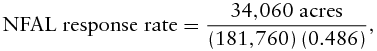 $$\begin{equation}
{\rm{NFAL\ response\ rate}} = \frac{{{34,}{060}\ {\rm{acres}}}}{{\left( {{181,}{760}} \right)\left( {0.486} \right)}},
\end{equation}$$
$$\begin{equation}
{\rm{NFAL\ response\ rate}} = \frac{{{34,}{060}\ {\rm{acres}}}}{{\left( {{181,}{760}} \right)\left( {0.486} \right)}},
\end{equation}$$
which yielded an estimate that 38.5% of NFALs in the watershed responded.
Respondents sometimes chose to skip questions, or others skipped the choice sets altogether on mail surveys. A total of 41 of the 67 producers and 36 of the 65 NFALs completed the best-worst section. Therefore, the overall response rate for this choice experiment was estimated to be 13.8% for producers and 21.3% for NFALs.
This response rate may be considered low and may be because of a variety of factors, including the use of an indirect list of property owners from an assessor's database, how we estimated the response rate based on agricultural census data, the administration of the survey by mail, or that fall is often a busy time for producers in the FCRW. Fall coincides with activities such as the optimal hard red winter wheat planting dates of late September through October (Epplin, Hossain, and Krenzer, Reference Epplin, Hossain and Krenzer2000) and the November Thanksgiving holiday. Furthermore, surveys of small businesses often have low response rates (Dennis, Reference Dennis2003); farmers and ranchers may be considered small businesses.
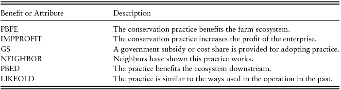
This study is part of a multidisciplinary research project conducted by a team of scientists from the USDA Agricultural Research Service in El Reno, Oklahoma, and from Oklahoma State University's Biosystems and Agricultural Engineering and Agricultural Economics departments. Using the literature review and input from the multidisciplinary grant team, six benefits or characteristics of a generic conservation practice were identified and included in the model. In Table 1, the benefits and characteristics of each attribute included in the best-worst scaling choice experiment are given with variable names and descriptions.
Table 1. Conservation Method Benefits and Attributes
6. Empirical Model
Finn and Louviere (Reference Finn and Louviere1992) first introduced the maximum difference scaling method, also called the best-worst scaling method. The method has since become an increasingly popular tool in many fields, including agricultural economics (Flynn et al., Reference Flynn, Louviere, Peters and Coast2007; Lusk and Briggeman, Reference Lusk and Briggeman2009; Lusk and Parker, Reference Lusk and Parker2009). The best-worst method forces the respondent to make a trade-off during each choice set, which more closely approximates how people make decisions and avoids bias caused from personal perception during analysis (Finn and Louviere, Reference Finn and Louviere1992). The terms best and worst in “best-worst” are not meant to convey that one attribute is always best and one always worst; rather, the terms refers to one attribute being least preferred and one being most preferred.
In this study, the respondents were asked to rank the most important reason for adoption of a conservation practice and the least important reason for choosing a practice in six separate choice sets. The first five choice sets included three reasons to adopt a conservation practice. In each of these five choice sets, the respondent was instructed to select a reason for conservation practice adoption that was the most preferred and another of the three choices that was the least preferred reason for adoption. In the last question, all six reasons were present. The fifth choice set containing six reasons for adoption of conservation allows the respondent to choose the reason for adoption that is their most preferred reason and the least preferred reason for adoption relative to all other possible reasons in the experiment. The respondents’ choices do not imply that certain conservation methods are better or more effective than others but reflect the perceptions of which reasons are most important to the respondents.
Maximum difference scaling is a way to elicit and rank preferences or attributes, the reasons for adoption in this study. Each respondent sees several choice sets that vary in the number of choices in each set, the present-absent design, or may use a balance complete block design (BIBD). In a BIBD, each choice set has the same number of choices, and each choice is represented the same number of times throughout the experiment. The present-absent design includes different numbers of choices in one or more choice sets. An example of a choice set from this survey is given in Figure 1. In each choice set, the respondent is asked to select the most important or most preferred attribute and also to choose the least important or least preferred attribute present in the choice set as a reason for adopting a conservation practice. Once the respondents complete all choice sets, their responses allow for an attribute to be ranked relative to the other attributes. Thus, results are given on a ratio scale. On the ratio scale, comparison of results between sample populations becomes much easier because there is one and only one way to make a choice, which eliminates perception bias concerning levels in other methods such as discrete choice experiments (Flynn and Louviere, Reference Flynn, Louviere, Peters and Coast2007).
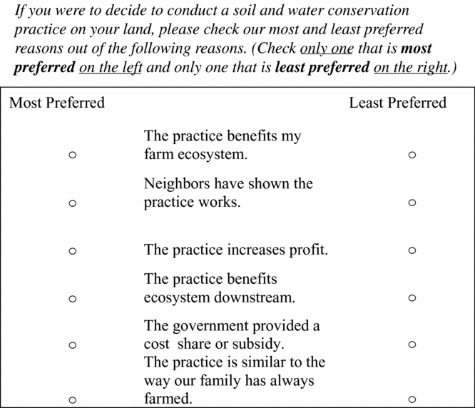
Figure 1. Example of Best-Worst Scaling Choice Set
In Table 1, the six benefits and characteristics of a conservation practice included in the model are described and listed. A 26 present/absent orthogonal design is used to design the choice sets; five of the choice sets include three benefits received from a conservation practice, and the last choice set includes all choices included in the experiment. The variable, “Practice benefits the ecosystem downstream” was slightly overrepresented in the design, because an attempt was made to discover how important an obvious externality is to landowners during adoption decisions. Both producers and NFALs were asked to choose which benefits of a conservation practice were most important or least important to them when making adoption decisions on their farm or farmland.
The best and worst choice (most and least preferred) reason to adopt a conservation practice in a choice set may be thought of as producers’ or NFALs’ preferences regarding incentives and the utility derived from adopting a practice on their operation or farmland, given programs such as CRP, CSP, EQIP, and so forth, or no program at all. Following Finn and Louviere (Reference Finn and Louviere1992) and Lusk and Briggeman (Reference Lusk and Briggeman2009), let λ j be the location of the Jth value on the scale of relative importance of the benefits or attributes of a conservation practice adopted, and the real or true level of importance of this λ j be Iij = λ j + ε ij , where ε ij is the error term such that it takes an extreme value distribution. The probability that the ith producer or NFAL chooses to maximize the distance between j and k—that is, as the best and worst out of J benefits of a conservation practice—is the probability that the difference in Iij and Iik is the greatest of all other possible values J(J − 1) − 1 possible differences in that choice set. Therefore, a model utilizing the conditional logit may be used:
 $$\begin{equation}
{\rm{Prob}}\left( {j\ {\rm{is\ most\ and}}\ k\ {{\rm least\ preferred}}} \right){\rm{\ }} = {\rm{\ }}\frac{{{e^{{\lambda _j} - {\lambda _k}}}}}{{\mathop \sum \nolimits_{l = 1}^j \mathop \sum \nolimits_{m = 1}^j \begin{array}{*{20}{c}} {{e^{{\lambda _l} - {\lambda _m}}}}&{ - J} \end{array}}},
\end{equation}$$
$$\begin{equation}
{\rm{Prob}}\left( {j\ {\rm{is\ most\ and}}\ k\ {{\rm least\ preferred}}} \right){\rm{\ }} = {\rm{\ }}\frac{{{e^{{\lambda _j} - {\lambda _k}}}}}{{\mathop \sum \nolimits_{l = 1}^j \mathop \sum \nolimits_{m = 1}^j \begin{array}{*{20}{c}} {{e^{{\lambda _l} - {\lambda _m}}}}&{ - J} \end{array}}},
\end{equation}$$
where m represents the benefits the producer or NFAL are presented but did not choose from the choice sets. Each best-worst possible pair is coded in SAS, using Proc MDC, where 1 is entered into the appropriate cell in a column representing the choice if chosen (SAS Institute, 2012). One variable, LIKEOLD, is dropped from the model to avoid perfect collinearity among the variables; this is the variable of comparison.
7. Results and Discussion
The descriptive statistics for producers are given in Table 2. According to the USDA's 2012 Census of Agriculture for Caddo, Washita, and Custer Counties (USDA-NASS, 2012a, 2012b, 2012c), approximately 51.4% of the land area is owned by agricultural producers and 48.6% is owned by NFAL. This indicates that the proportion of NFAL and producer respondents from our sample is consistent with the USDA statistics given that 50.8% of respondents are producers and 49.2% of respondents are NFALs. Because this survey includes both ranchers and farmers of crops such as grains, cotton, and soybeans and does not target farmers of specific crops, any respondent producing agricultural commodities or products is termed a producer. The average farm operation for producers responding to the best-worst choice set is 1,012 acres, and the average amount of farmland owned is 639 acres, with a median acreage of 400 acres (Table 2). The average farmer has 30.1 years production agriculture experience, and approximately 15% of respondents are female. Producers identify by race as 92.7% white and 7.3% Native American. Average annual total farm revenue is $138,780 per annum, with a median of $122,500. Sixty-one percent of producers participate in at least one conservation program. The summary statistics of the sample data were compared with the average values found in the USDA's 2012 Census of Agriculture for Caddo, Custer, and Washita Counties (USDA-NASS, 2012a, 2012b, 2012c), which bound the Fort Cobb Watershed. According to the USDA, in 2012 the average total farm revenue was $107,906 per annum. The average age of a producer was 57 years, and 95.9% of the farming population was white, 3.3% was Native American, 0.8% identified as another race, and 7.4% was female. The average farm size in acres for these three counties was 615 acres. Overall, the survey data from the FCRW included operations slightly larger than the average farm size indicated in the USDA's 2012 Census of Agriculture for both measures in land mass and total revenue. Females were overrepresented by approximately double compared with the data from the USDA data. Assuming the average beginning age upon entrance to the production agriculture sector was 23, allowing for postsecondary education attainment, then the age of the average farmer was very close to those listed in the USDA data. The distribution of respondents’ identification to racial group was also similar to the USDA's 2012 Census of Agriculture.
Table 2. Descriptive Statistics for Producers in the Fort Cobb Reservoir Watershed in 2014Footnote a
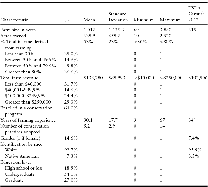
a n = 41 with exception of education variables, where n = 37.
b Source: U.S. Department of Agriculture's (USDA) 2012 Census of Agriculture.
c USDA producer experience is calculated assuming an average age of entry at 23 years.
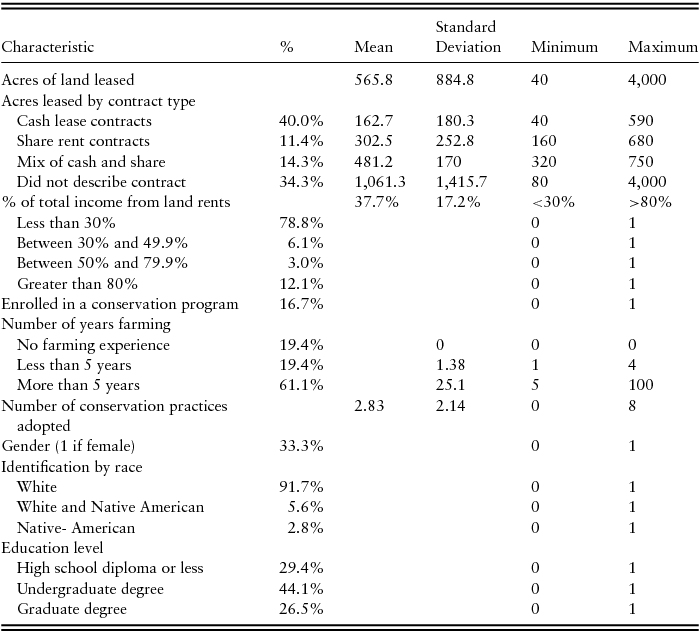
The descriptive statistics for the NFAL are given in Table 3. There were no publicly available data with which to compare the demographics of NFAL in the sample. Of those responding, the average amount of farmland leased was approximately 566 acres, with a median value of 198 acres. Forty percent of respondents indicated they rent the land on a cash-rent basis. Eleven percent stated they use a share-rent contract, 14% percent lease farmland using both cash-rent and share-rent contracts, and 34% did not specify the nature of the lease agreement. Most NFALs receive less than 30% of their total income from rents and only 17% own land enrolled in a conservation program. Approximately 19% indicated they had no farming experience, and 19% indicated they had less than 5 years of farming experience. Female respondents represented 33% of the NFAL sample, and the distribution of racial identification was similar to the makeup of the producers. Less than one-third of the respondents indicated that the highest level of education they had obtained was a high school diploma or less, while 44% had completed undergraduate studies, and almost 27% had obtained a graduate degree. We can hypothesize that because the higher education levels of producers versus NFALs were similar (80.1% and 70.6% have undergraduate or higher degrees, respectively), lack of educational attainment was not the reason for NFALs being less likely to value government subsidies. However, the NFALs had a much higher proportion of less or completely inexperienced farmers and women for whom we tentatively hypothesize that off-farm opportunities were greater, meaning conservation payments were of less importance.
Table 3. Descriptive Statistics for Nonfarming Absentee Landowners, Fort Cobb Watershed
The watershed does not appear to follow the national trend in which NFALs are increasing over time; instead, they remained relatively constant in the FCRW. Approximately 48.6% of land in the FCRW was owned by NFALs (USDA's 2012 Census of Agriculture). The USDA's Census of Agriculture in 2002 and 2007 indicate that 48% and 46% of the area was owned by NFALs (USDA-NASS, 2002, 2012d). Even though the FCRW does not follow the national trend that NFALs are increasing over time, because they represent almost 50% of the landownership in the area they are an important to consider when developing appropriate agricultural policy.
Table 4 gives the raw data describing the choices made by all individuals in each model. The entries in the “Best” column indicate how many times the respondents chose that benefit or characteristic of a conservation practice as most preferred, and the entries in the “Worst” column give the total number of times that variable was chosen as the least preferred. By simple visual inspection of this table, one will see that producers chose IMPPROFIT more times than any other choice as the most preferred reason to adopt a conservation practice, so intuitively one may come to the conclusion that IMPPROFIT is the most preferred reason to adopt a conservation practice for producers overall. However, this intuitive conclusion is not always correct. A somewhat simplified explanation of the power of the best-worst method for this type of application is that in essence this method considers the distances between the likelihood of a specific reason or attribute being chosen as most preferred and least preferred and uses this distance as a “weighting” of that factor and its importance relative to all other choices. This point is illustrated in Table 5 in that the results of the best-worst econometric model show that the intuitive conclusion concerning IMPPROFIT is incorrect and that producers actually prefer PBFE as the most preferred reason to adopt a conservation practice.
Table 4. Frequency of Best or Worst Rating for Each Attribute
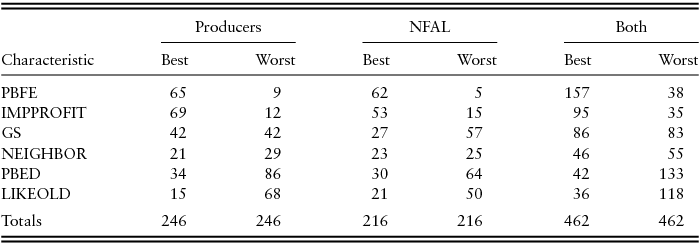
Notes: NFAL, nonfarming/absentee landowners.
Table 5. Relative Importance of Soil and Water Conservation Attributes
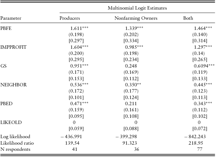
Notes: Asterisks (*, **, ***) represent the 90%, 95%, and 99% confidence levels, respectively. Standard errors are reported in parentheses. No standard error reported for the dropped variable LIKEOLD. Importance scores are in square brackets. Log likelihood test statistic was 11.9; the chi-square critical value for the 95% level is 11.1.
The model estimates are given in Table 5. For the multinomial logit (MNL) estimates, the higher the parameter estimate, the more preferred the benefit or attribute of the conservation method was compared with other benefits and attributes with a lower MNL parameter value. Standard errors are reported in parentheses. Importance scores are given in brackets and may be interpreted as the fraction of each group that would choose that category as the most important relative to the other options. The preferences are given a numerical ranking, and the importance score is converted to a percentage in Table 6. This importance score in percentage form may be interpreted as the percentage of members of the respective group expected to choose the attribute or benefit as most preferred.
Table 6. Preference Shares by Producer, Nonfarming Landowner, and Pooled Model

Notes: Asterisks (*, **, ***) represent the 90%, 95%, and 99% confidence levels, respectively. Relative rank reported with numerals 1–6. Importance scores are converted to percentage and presented with % following the numeral.
The producers and NFALs have different preference orders compared with each other. The difference in preference rankings and order is shown in Figure 2, along with the difference in the magnitude of the MNL estimates between the two groups. Figure 3 graphically presents the importance scores, which are percent of the respondents who prefer each attribute as the most desirable reason to adopt a conservation practice. The importance score is calculated as follows:
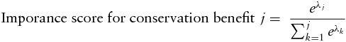 $$\begin{equation}
{\rm{Imporance\ score\ for\ conservation\ benefit}}\ j = \ \frac{{{e^{{\lambda _j}}}}}{{\mathop \sum \nolimits_{k = 1}^j {e^{{\lambda _k}}}}}
\end{equation}$$
$$\begin{equation}
{\rm{Imporance\ score\ for\ conservation\ benefit}}\ j = \ \frac{{{e^{{\lambda _j}}}}}{{\mathop \sum \nolimits_{k = 1}^j {e^{{\lambda _k}}}}}
\end{equation}$$
where, λ j is the MNL estimate for the jth benefit of a characteristic of a conservation practice and λ k represents the MNL estimates for the kth benefits and characteristics of conservation practices. The importance score may be interpreted as the expected proportion of the population that would choose that benefit or characteristic of a conservation practice as most preferred.
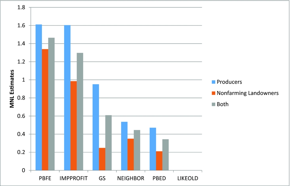
Figure 2. Best-Worst Multinomial Logit (MNL) Relative Importance Estimates
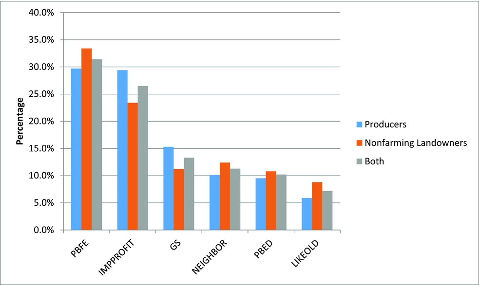
Figure 3. Preference Shares for Highest Importance of Attributes
Brady and Nickerson (Reference Brady and Nickerson2009) assert that producers and absentee landowners respond differently to incentives. In the study, the likelihood ratio test yields a test statistic of 11.9 for the pooled model, and the critical value associated with the 95% level with five parameter values is 11.1. Therefore, the log-likelihood test shows that at the 95% level, producers and NFALs have different preferences during adoption than producers, supporting the hypothesis that producers and NFALs have significantly different overall preference orderings (Table 6).
The importance score may be interpreted as the proportion of the population that will choose that benefit or characteristic of a conservation practice as most important. The most important factor for both producers and NFALs when making adoption decisions was whether the practice benefits the farm ecosystem (PBFE). Although this result conflicts with the hypothesis that IMPPROFIT would be the most desirable benefit derived from a practice for producers, the importance score indicates that only 0.3% of producers in the FCRW chose this category over profit. This likely reflects the common colloquialism that if “you take care of the land, it will take care of you.” However, despite the ranking of the two choices being the same, NFALs have a much larger margin between the PBFE and IMPPROFIT. The NFALs choose the PBFE as the most desirable characteristic of an adoption decision by a 10% margin over IMPPROFIT. This may indicate that NFALs are more interested in the long-run profitability of the enterprise based on both profit and ecosystem benefits than agricultural producers.
To further demonstrate the differences between the two groups, the order of the rankings of the next two attributes are not the same; although it is of note that GS is not found to be significant for NFALs, the order is still important. Producers rank GS and NEIGHBOR as the third and fourth best choices, respectively. The importance score for GS is chosen as most important 15.3% of the time, and NEIGHBOR 10.1% of the time. NFALs rank these attributes in an opposite fashion than the producers in that they prefer NEIGHBOR 12.4% of the time over 11.2% for GS. This may indicate that information, incentives, and educational efforts concerning government programs fail to motivate or reach NFALs as effectively as producers who live in the FCRW, which reinforces the findings of Petrzelka, Buman, and Ridgely (Reference Petrzelka, Buman and Ridgely2009).
One hypothesis was that the least important reason to adopt a practice for both groups was if the practice benefits the ecosystem downstream. Although the order of PBED and LIKEOLD is not the same as the hypotheses, these two characteristics both come in last. PBED came in as the fifth most important factor with 9.5% of producers and 10.8% of NFALs choosing this as the most important factor, although for NFALs the MNL estimate was not significant compared with the dummy variable LIKEOLD. LIKEOLD was least preferred, with 5.9% of producers and 8.8% of NFALs choosing this attribute as the best reason to adopt a practice. Although the low ranking of PBED for both groups is discouraging, at least both groups are also not interested in maintaining older, status quo methods that may contribute to erosion.
8. Summary and Conclusions
The findings of this study are useful for educational efforts geared toward engaging absentee landowners. Furthermore, findings are useful for policy makers when developing new incentive types for both producers and NFALs. The study shows agricultural producers value protecting the environment both on- and off-farm. This indicates they are aware that conventional farming methods may negatively affect the environment. Many prefer stewardship to practices that are not likely to be environmentally sustainable.
Benefit to one's own farm ecosystem is the primary reason both producers and NFALs support adoption of a specific practice. For the most part, producers view practice adoption differently than absentee owners. A larger proportion of producers are driven by short-run profit considerations than nonfarming absentee landowners. Producers rank a government subsidy or cost share as the third most important reason for adopting new methods. NFALs rank government subsidy as the fourth best reason, although in the MNL estimate it proved insignificant compared with the dropped dummy variable. This result suggests that government subsidies and cost shares benefit absentee landowners less than producers, or that NFALs are not aware of the on-farm benefits of the conservation programs. Absentee owners are more interested in the long-term rents obtained from the land than producers whose incentives are tied more strongly to the present (Boumtje et al., Reference Boumtje, Barry and Ellinger2001).
Therefore, to provide appropriate and effective incentives to both groups, this research supports the findings of Camboni and Napier (Reference Camboni and Napier1993), Dobbs and Pretty (Reference Dobbs and Pretty2004), and Shortle et al. (Reference Shortle, Ribaudo, Horan and Blanford2012) in the assertion that the current incentive system may need restructuring. Programs may be developed and tailored to the preferences of the land tenure groupings. This will encourage both groups to reduce external production effects caused from current agricultural practices and reduce production losses caused by outdated methods. To the extent that further research indicates some conventional practices cause negative externalities, the results of this study support the need for education programs to target both producers and landowners. As a result, the benefits of government-supported conservation programs could enhance participation rates, thus reducing the losses society.


 Open access