


1. Introduction
In indirect laser driven inertial confinement fusion (ICF), laser–plasma interaction between the laser and the hohlraum wall produces X-rays, and the X-rays drive the pellet to implosion[Reference Brueckner and Jorna1–Reference Lindl3]. It is easy to achieve uniform irradiation of the target surface due to repeated absorption and re-emission of X-rays constrained by the hohlraum. However, there is a transition time to achieve uniform irradiation. The better the initial irradiation uniformity is, the shorter the transition time is. So obtaining high uniformity of the initial irradiation is the key to achieving implosion[Reference Hauer, Suter, Delamater, Ress, Powers, Magelssen, Harris, Landen, Lindmann and Hsing4,Reference Tsakiris5] . As initial irradiation evenness is determined by the optical intensity distribution on the hohlraum[Reference Nakamura, Kondo, Nishimura, Endo, Shiraga, Miyamoto, Kato and Nakai6,Reference Lai and Feng7] , it is necessary to study the optical intensity distribution on the hohlraum wall. At the same time, the parametric instability process in the laser–plasma interaction (LPI) affects the laser–hohlraum target coupling efficiency and further influences the laser–pellet coupling efficiency, which creates a negative impact on the laser fusion[Reference Kruer and Dawson8,Reference Sprangle, Esarey and Ting9] . The LPI process is a key link in the laser fusion research, which is closely related to the initial laser conditions[Reference Froula, Divol, London, Berger, Döppner, Meezan, Ralph, Ross, Suter and Glenzer10]. Therefore, extensive research about the optical field distribution on the hohlraum wall[Reference Xu and Lv11–Reference Huang, Yao, Zhao, Zhang, Wu and Gao15] and related LPI process[Reference Gibbon and Förster16–Reference Umstadter20] is being carried out both here and aboard. However, usually only the steady state in the flat period of a flat-topped pulse is considered. The flat-topped pulse is treated as an ideal rectangular function. But the flat-topped pulse in actual ICF physics experiments has a rising edge of picosecond (ps) order. And physics experiments are generally more concerned about the features at the rising edge of the pulse period. Because of the oblique incidence to the hohlraum, there is a time difference of picosecond order between different hohlraum wall positions. So the pulse laser’s irradiating to the hohlraum wall is actually a push-broom process. The optical field changes swiftly during the rising edge and the instant optical intensity distribution on the hohlraum wall becomes quite different from the steady state. This kind of difference may bring great impact on the LPI physical process. Without consideration of this difference, there will be such a big deviation compared to the physical truth, which may keep us away from a deeper understanding and finer analysis of related physical problems. Accordingly, using a conventional fast Fourier transform (FFT) method combined with the chromatography principle[Reference Huang, Yao, Zhao, Zhang, Wu and Gao15], the spatial distribution changes of the optical field over time are analyzed in detail, which aims to provide a simple but finer and more comprehensive model of spatio-temporal optical intensity for LPI research.
2. Model and theory
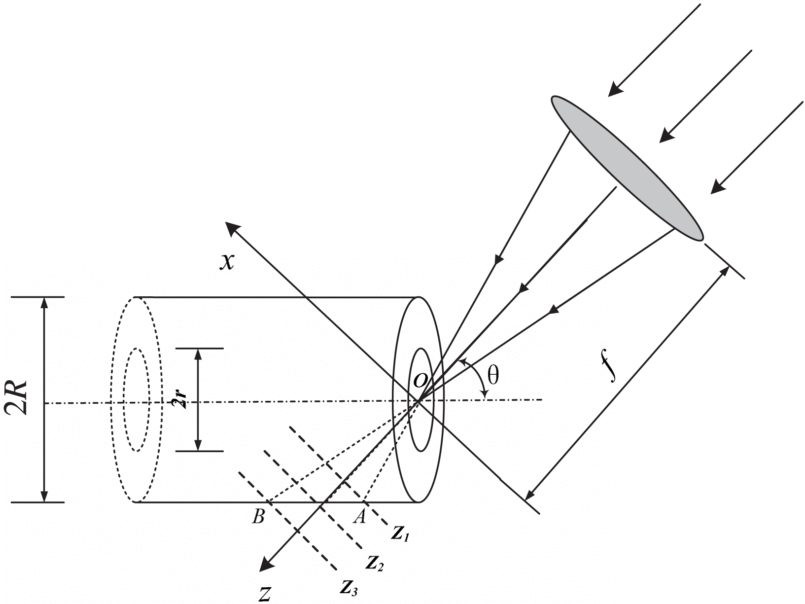
According to the national ignition facility’s target chamber structure model, the parameters of the final target chamber structure are as follows: laser wavelength  $\lambda = 0. 351~\unicode[.5,0][STIXGeneral,Times]{x03BC} \text{m} $, beam size $400~\mathrm{mm} \times 400~\mathrm{mm} $, 10-order super-Gaussian beam with waist radius $\omega = 160~\mathrm{mm} $. After passing through a lens with focal length $f= 7700~\mathrm{mm} $, the laser beam passes through the orifice with diameter $2r= 3. 5~\mathrm{mm} $ into a cylindrical target chamber with diameter $2R= 15~\mathrm{mm} $, as shown in Figure 1. Here the optical field distribution on the inclined cylindrical surface ( $\theta = 23. 5{{}^\circ} $) is mainly of interest. According to the calculation model based on chromatography theory from the literature[Reference Huang, Yao, Zhao, Zhang, Wu and Gao15], we calculate the multi-plane optical field to fit the optical field on the cylindrical surface. Divide the diffractive area into enough near planes perpendicular to the light propagation direction, as shown in Figure 1. The optical field is calculated in each plane to get a homogenized three-dimensional diffraction field data grid at equal intervals in $x, y$, and $z$ directions. Finally, in accordance with the principle of ‘the most adjacent’ principle, the optical field on the cylindrical surface is fitted from three-dimensional data[Reference Huang, Yao, Zhao, Zhang, Wu and Gao15]. The $z$-direction represents the beam propagation direction (i.e., the focusing lens central axis), the $x$-direction is perpendicular to the $z$-direction in the paper plane, and the $y$-direction is perpendicular to the paper plane.

Figure 1. Diagram of ICF target chamber device and chromatography.
Based on the model shown in Figure 1, when the angle between the optical axis and the cylindrical axis equals  $23. 5{{}^\circ} $, the distance between $A$ and
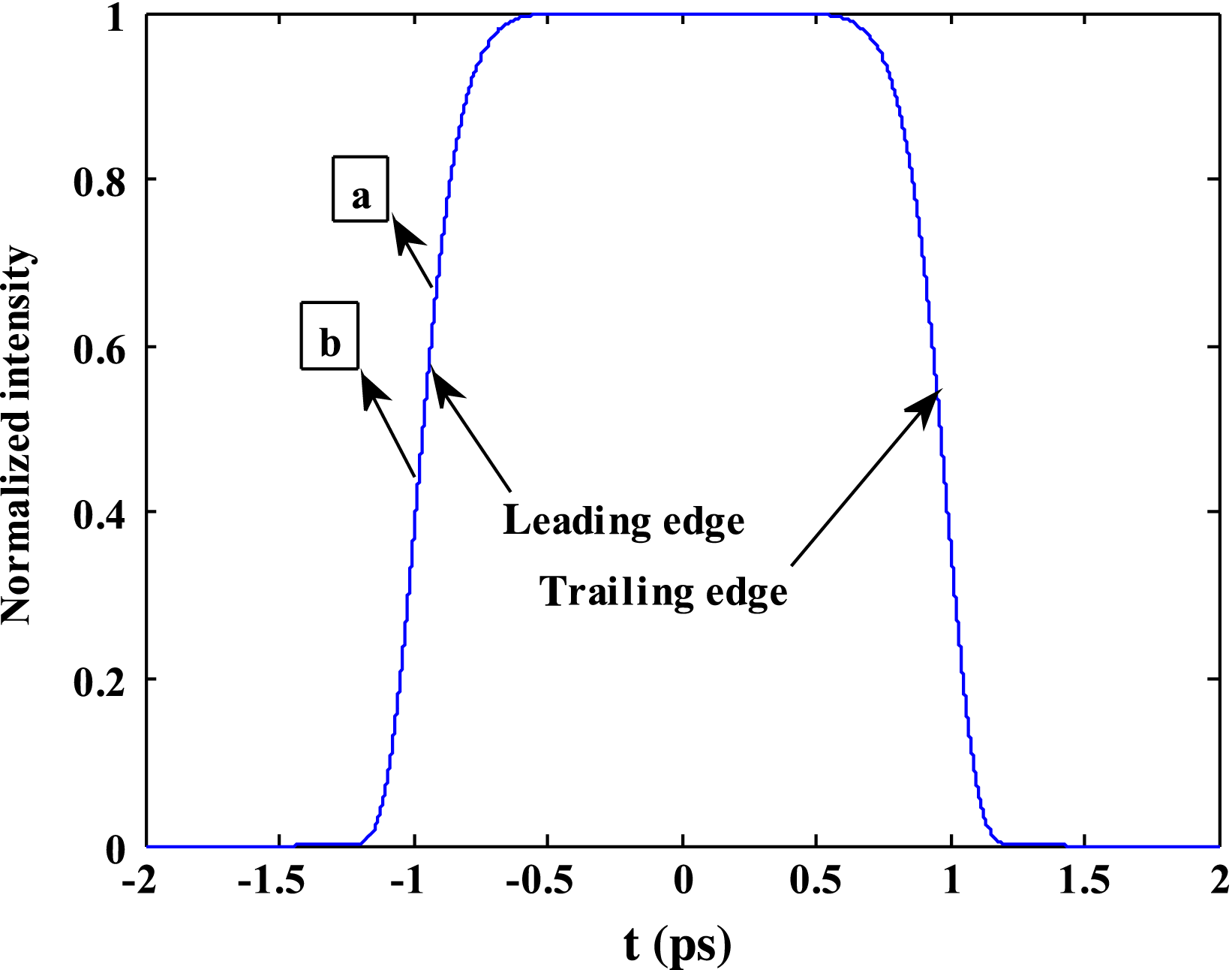
  $B$ along the optical axis is 2.25 mm, and the corresponding time difference is approximately 7.64 ps. So, taking into account of the propagation characteristics of the pulse time, there is a certain time delay between different positions. If the pulse is divided into a series of time sequences, at the same moment different time sequences arrive at different spatial positions on the wall of hohlraum. As shown in Figure 2, in a flat-topped pulse, at the same instant the remote location $B$ corresponds to the front pulse sequence position of point $b$ and the closer position $A$ corresponds to point $a$. The intensities of different pulse sequences are different. As for the rising edge, the optical intensity of sequence $b$ is larger than that of sequence $a$; then it is deduced that at the same time the optical intensity of the pulse sequence corresponding to position $A$ is bigger than that of $B$. During the rising edge of a picosecond order in a flat-topped pulse, optical intensity differences between $A$ and $B$ due to a time delay of picosecond rate will become more obvious.
Figure 2. Pulse sequences corresponding to positions  $A$ and $B$ at the same instant.
3. Simulation and analysis
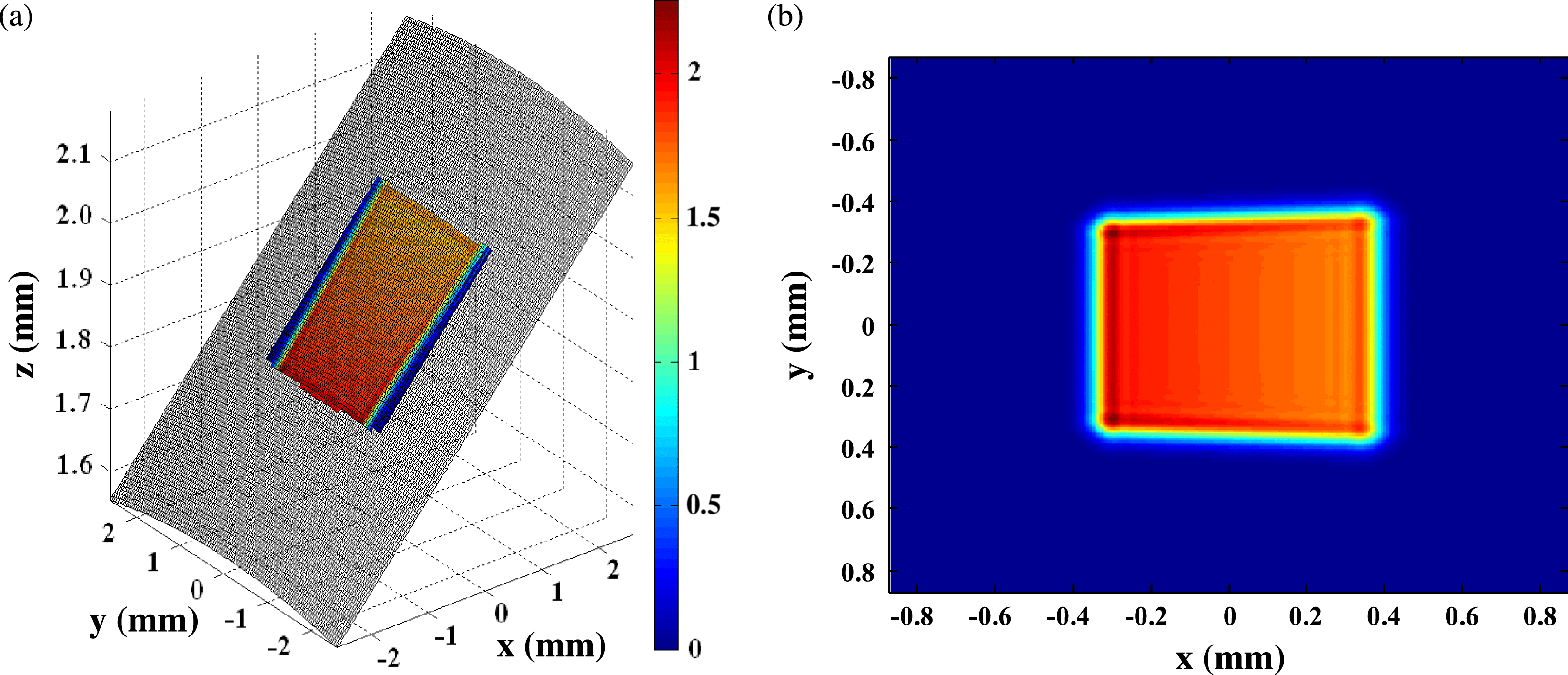
Based on the above model and computing method, first the optical field in the steady state is analyzed. The three-dimensional intensity distribution on the cylindrical surface is shown in Figure 3(a). For convenience of analysis, the projection view of the cylindrical optical field in  $xoy$ plane is shown in Figure 3(b). It is shown that the projection shape is not rectangular, but similar to a trapezoid.
Figure 3. (a) Optical field distribution on the cylindrical surface; (b) projection in  $xoy$ plane.
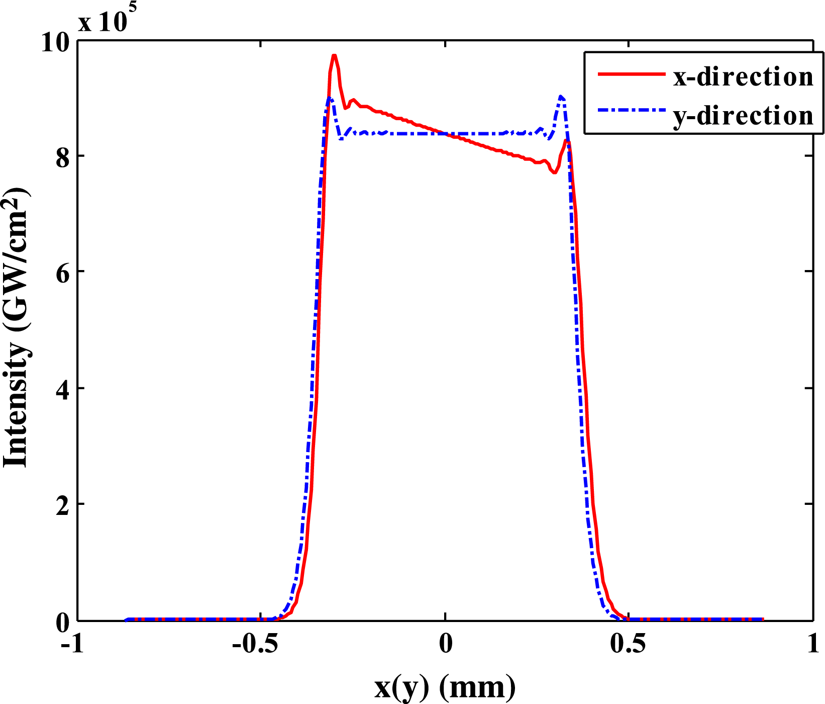
The optical field distribution both at  $y= 0$ and $x= 0$ extracted from the projection is shown in Figure 4. As can be seen, the optical intensity distribution along the $y$-direction distribution is symmetric and the optical intensity distribution along the $x$-direction is asymmetric. When the super-Gaussian beam is focused through a lens, the minimum spot size and the maximum intensity are obtained at the focal point. With increasing distance away from focus of the lens, the beam size is increased and the optical intensity is decreased, so an asymmetric distribution appears in the $x$-direction.
Figure 4. Optical intensity distribution along the  $x$ and $y$ directions.
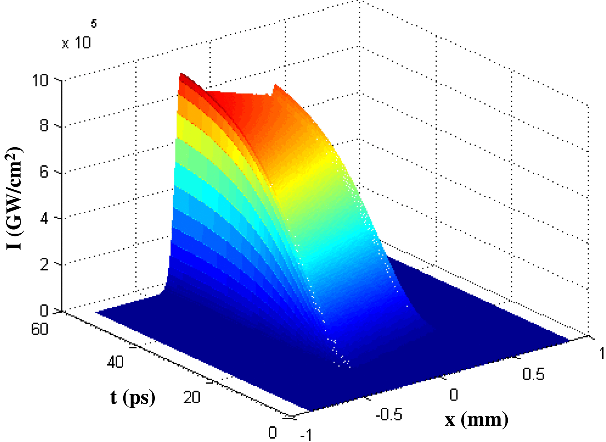
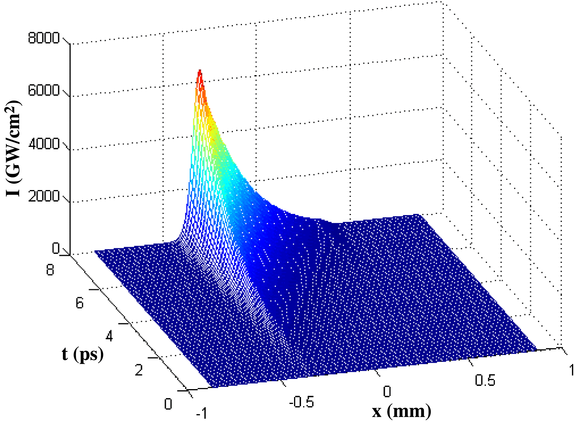
When considering the temporal characteristics of the laser pulse, 50-order super-Gaussian pulses with pulse width  $T$ of 1 ns and a rising edge of approximately 50 ps are taken as examples. The optical field distribution changes with time on the hohlraum wall are simulated, as shown in Figure 5. We extract the optical field distribution along the $x$-direction in the first 8 ps, and the results are shown in Figure 6. At the same instant, when the distance from the lens is less (smaller $x$), the optical intensity is stronger. The time delay between $A$ and $B$ is approximately 7.6 ps. In the initial 7.6 ps of the pulse, the intensity of position $A$ increases rapidly over time, but light reaches position $B$ at a later time with quite a small optical intensity. This is because the rising edge of this pulse is very steep; even though the time delay of 7.6 ps is very short, the intensity of position $A$ still experiences a huge increase. This leads to a big difference of the optical intensity between positions $A$ and $B$ at the rising edge of the initial 7.6 ps. As a result, the energy deposited in position $A$ is much larger than in position $B$ in the initial 7.6 ps. After the initial 7.6 ps, the optical intensity at position $B$ starts to increase as time goes on and the difference between $A$ and $B$ becomes gradually smaller. If we only consider the steady state of the optical field distribution to analyze the laser–plasma interactions and other related physical processes, there will be a obvious deviation from the actual situation. The change in the distribution of the optical field along the
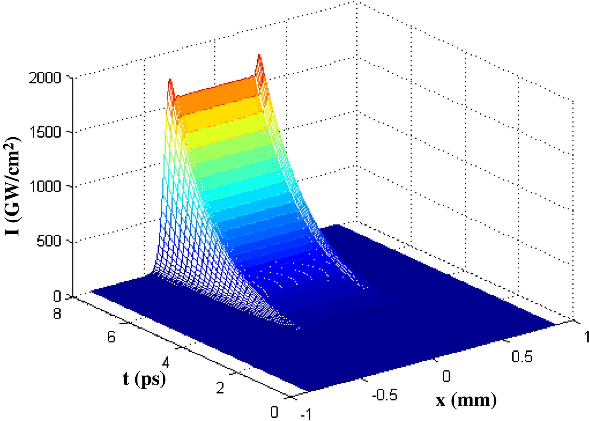
  $y$-direction within the initial 8 ps is shown in Figure 7. As is analyzed above, the optical intensity distribution along the $y$-direction is symmetrical. The intensity for each position increases as time goes on, but the overall distribution does not change over time.
Combining the optical field changes over time in both the  $x$ and $y$ directions, we can see that the optical distribution on the hohlraum wall is a complex spatio-temporal evolutional process. In Figures 5–7, $t$ represents different instances in the rising edge of pulses while $I$ represents the optical intensity.
Figure 5. Spatio-temporal intensity distribution along the  $x$-direction on the rising edge.
Figure 6. Spatio-temporal distribution along the  $x$-direction in the initial 8 ps.
Figure 7. Spatio-temporal distribution along the  $y$-direction in the initial 8 ps.
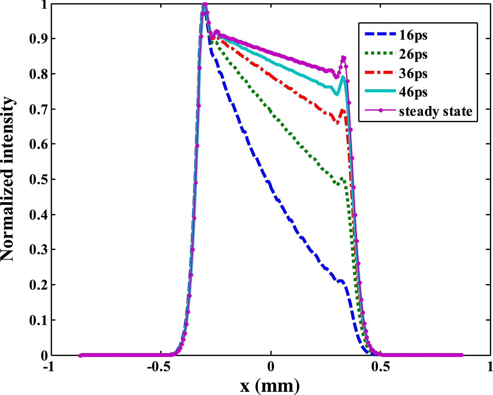
Because of the particularity of spatial and temporal changes in the  $x$-direction of the optical field, the optical field along the $x$-direction is carefully analyzed in the following. Parameter ${t}_{0} $ represents the pulse sequence in a pulse when it reaches position $A$ in the hohlraum wall. Compare the optical field in the steady state and unsteady state with different ${t}_{0} $ on the rising edge in Figure 8, where ${t}_{0} $ represents 16, 26, 36, 46 ps and a steady-state situation. Figure 8 shows how the instantaneous optical field distribution changes in different moments of the rising edge. The optical intensity of position $B$ is gradually approaching that of position $A$, and the whole optical field distribution tends to a steady-state distribution over time. In order to evaluate changes in the degree of inclination of the optical field distribution, we define the relative ratio $(R)$ of the optical intensity of positions $B$ and $A$ as follows:
 $$\begin{eqnarray}R= {I}_{B} / {I}_{A} ,\end{eqnarray}$$
 where  ${I}_{B} $ and ${I}_{A} $ represent the intensity of position $B$ and the intensity of position $A$, respectively.
When  $R$ is small, the intensity difference between $A$ and $B$ is greater and the optical field distribution is more tilted. When $R$ is large, the optical field distribution is more flat. For the steady state,
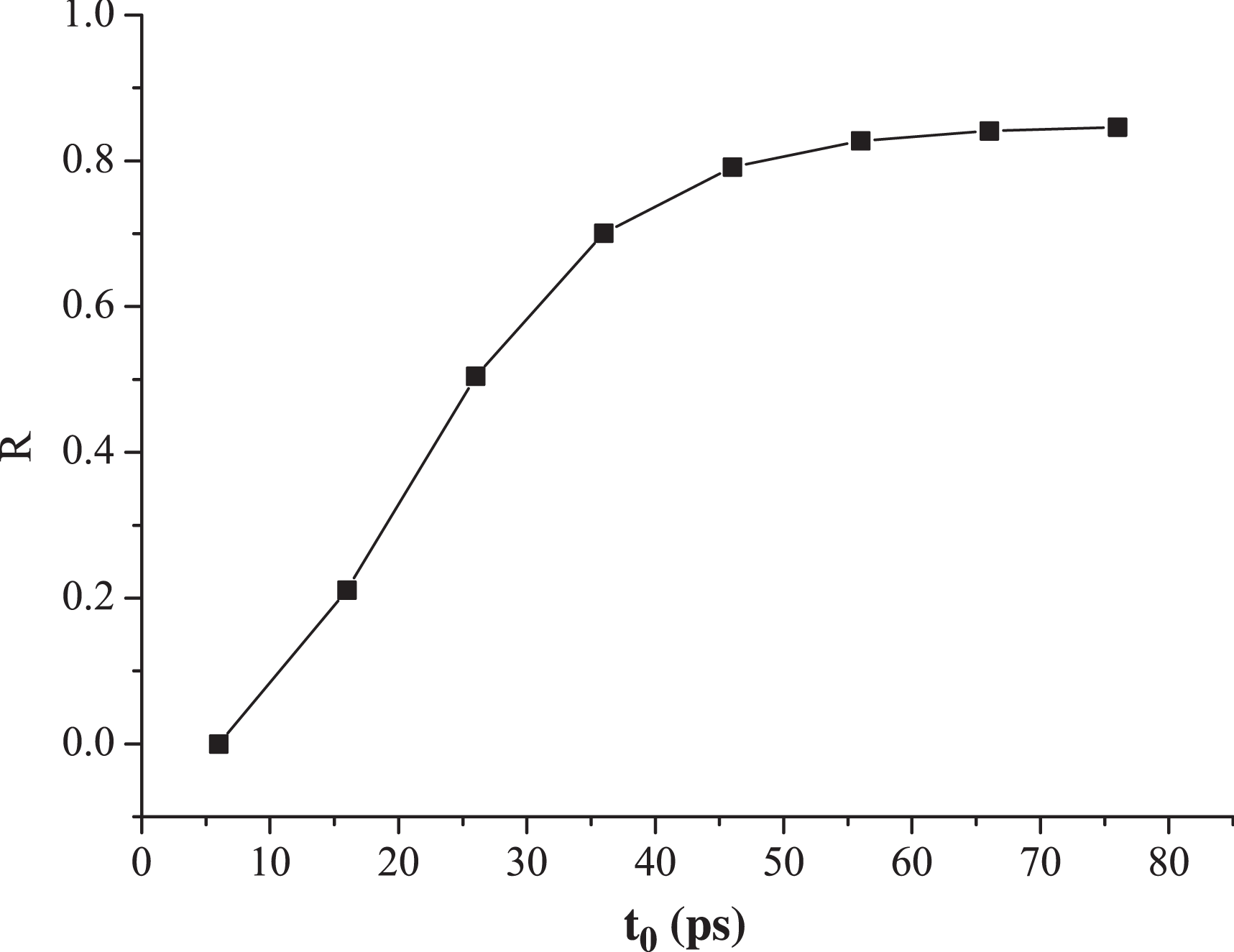
  $R$ equals 0.849. Figure 9 shows how $R$ changes with different ${t}_{0} $ on the rising edge, which reflects the degree of inclination of the optical field at different moments. As time goes by, $R$ gradually becomes larger and approaches a steady state, which means that the optical field is more and more flat. In other words, the optical field distribution tilts more seriously in the earlier moments on the rising edge and the optical field distribution is much closer to the steady-state distribution in the later moments.
Figure 8. Optical field distribution along the  $x$-direction at different moments of the rising edge.
Figure 9. Relative ratio of the optical field at different moments of the rising edge.
When different pulse sequences reach the hohlraum wall, the instantaneous optical field distribution changes a lot. Compared to the steady-state distribution, the optical intensity in the front position is larger than in the rear position and  $R$ gradually becomes larger at the rising edge. But in the flat-top region of the pulse, the optical field distribution is the same as that in he steady state, and the distribution does not change over time. As temporal characteristics of the rising pulse affect the optical field distribution a lot, the effect of steepness of the rising edge on the optical field changes over time is studied in the following research. We regard the rising edge model as a simple linear model,
 $$\begin{eqnarray}I= {I}_{0t} / {t}_{d} ,\end{eqnarray}$$
 where  ${t}_{d} $ is the length of the rising edge of the pulse. In order to focus on the role of time delay of different positions on the hohlraum wall and ignore the impact of different initial optical intensity on the optical field distribution on the rising edge, we choose to simulate the optical field at time
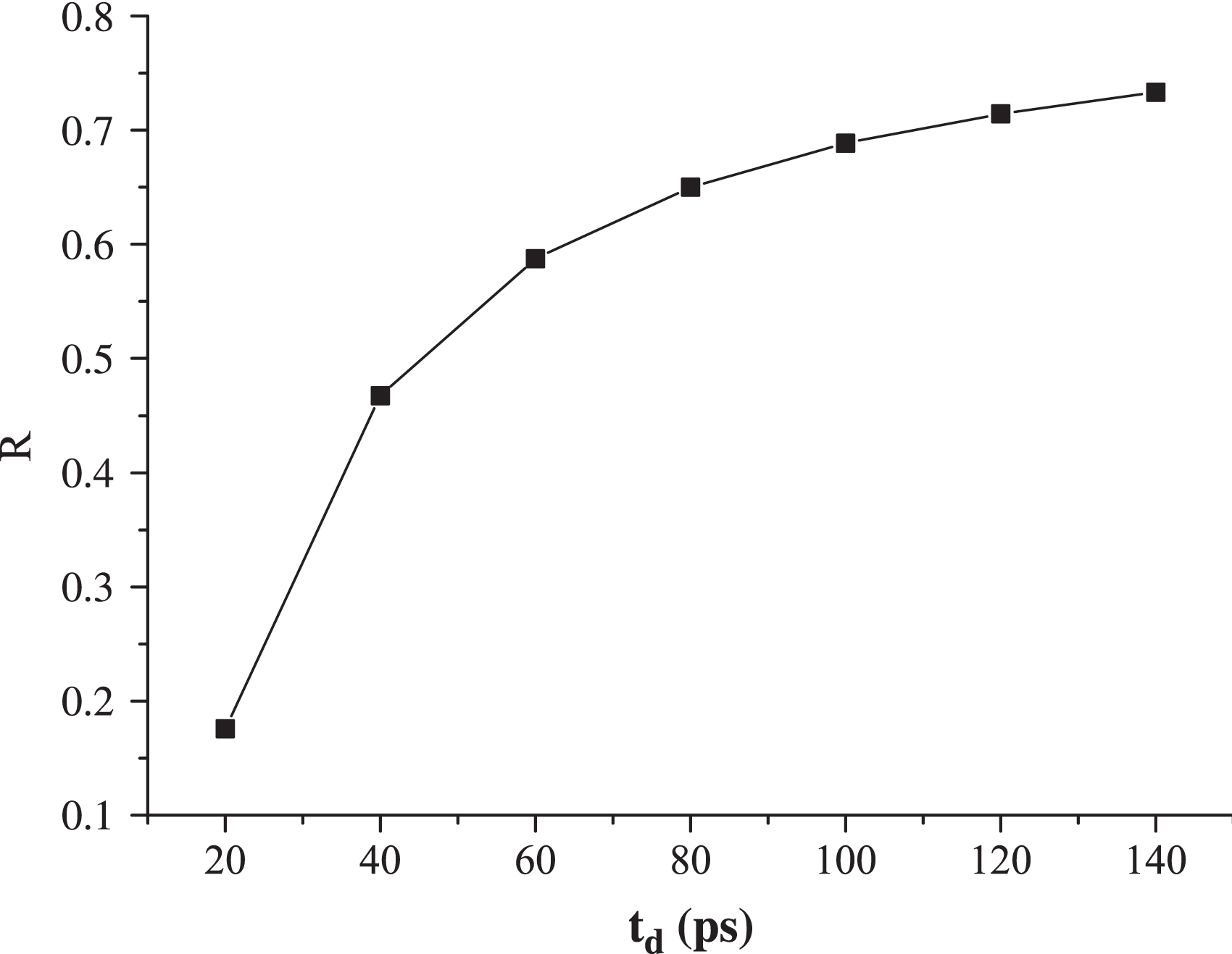
  ${t}_{0} = {t}_{d} / 2$ with different time length of rising edge, shown in Figure 10. We can see from the picture that, when ${t}_{d} $ is larger, the relative ratio $R$ is bigger and the optical intensity distribution is more flat and much closer to the steady state. When ${t}_{d} $ is smaller, the difference between the optical field distribution on the rising edge and the steady state is greater, which means that the optical field distribution changes more intensely with time. This is because, when the rising edge is much steeper, the optical field of the pulse changes more rapidly over time itself and the initial intensity difference of the pulse sequence caused by the arriving time difference is greater, resulting in a greater difference between the optical field distribution on the rising edge and the steady state. If the rising edge width is too long, this kind of spatio-temporal effect is too weak to be noticed.
Figure 10. Relative ratio of the optical field with different  ${t}_{d} $.
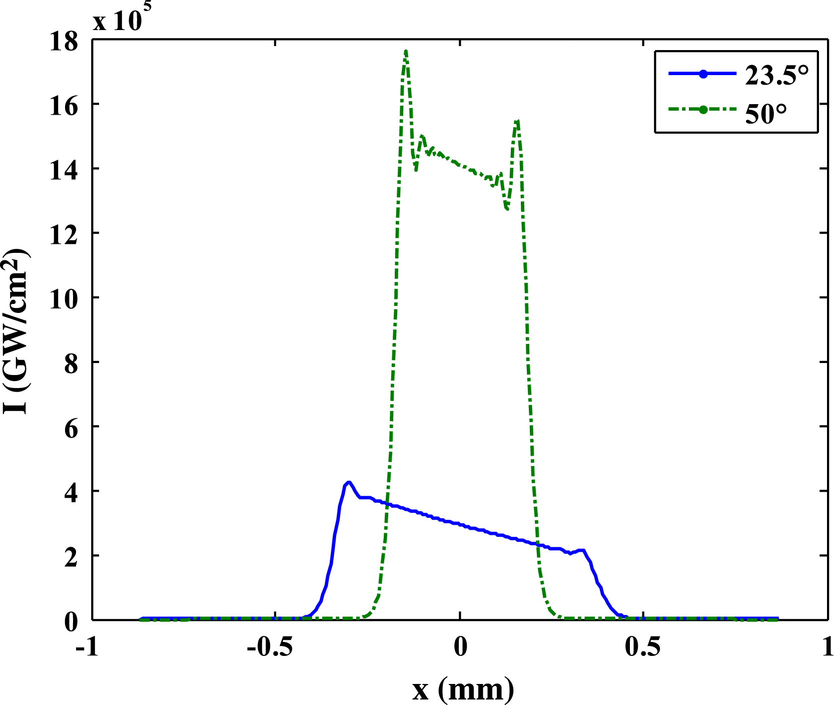
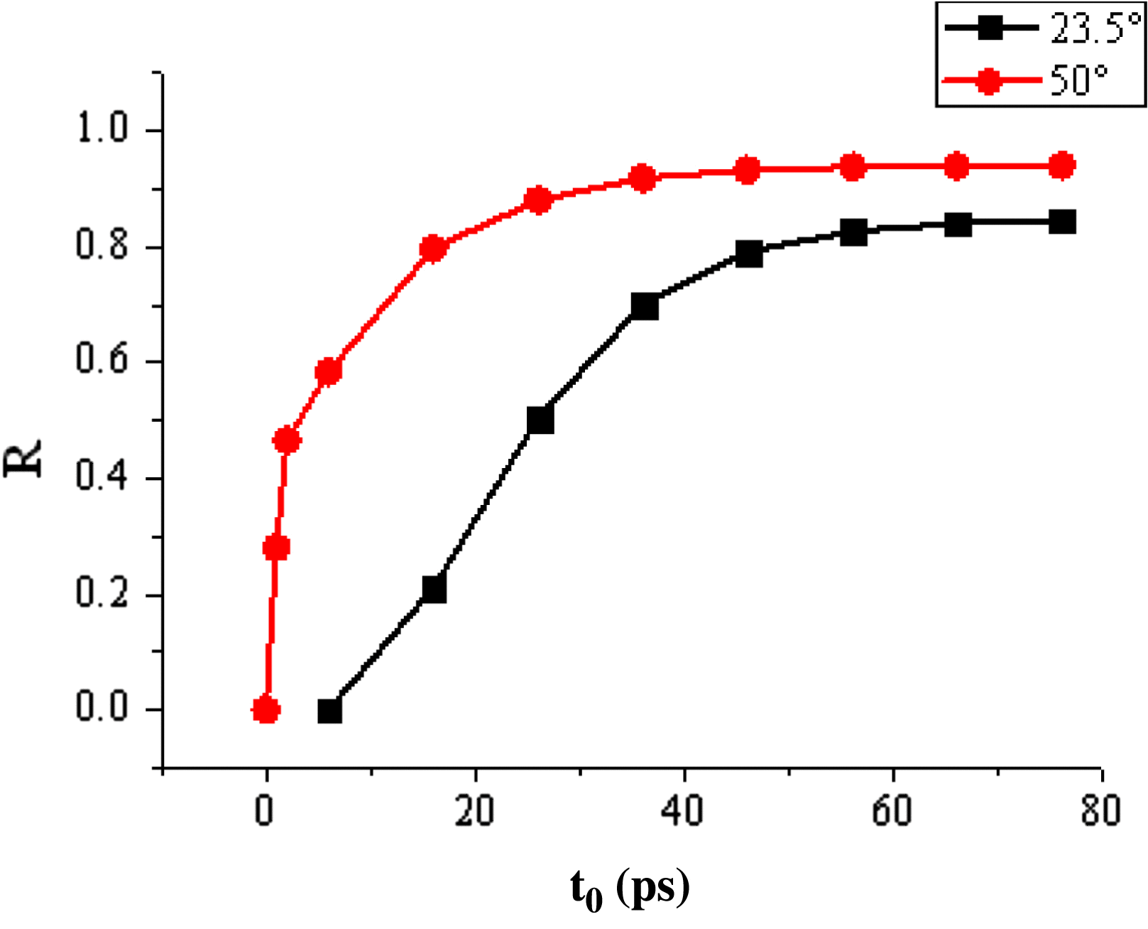
Incidentally, the incident light has different angles ( $\theta )$ of inclination with respect to the central axis of the hohlraum, the inner ring of 23.5°and 30°, and the outer ring of 44.5°and 50°. For the above-mentioned discussion, the optical field on the inner ring of 23.5° is analyzed as an example. Actually, the optical field on the inner and outer rings and its evolution at the rising edge are different. For different inclination angles, the laser strikes different locations on the hohlraum wall with various power densities and time delays; thus their temporal and spatial distributions are disparate. Specifically, when $\theta $ is smaller (for inner ring), the average power density on the hohlraum wall is smaller, as shown in Figure 11. And the time delay for different positions on the hohlraum wall is greater; thus the difference of optical field distribution at the same instance between the rising edge and the steady state is bigger and the spatio-temporal evolution of the optical intensity tends to the steady state more slowly, as shown in Figure 12. Therefore the spatio-temporal effect is more significant.
Figure 11. Optical field distribution for different inclination angles at the same instance.
Figure 12. Relative ratio of the optical field at the rising edge for different inclination angles.
4. Conclusion
To conclude, based on the time delay of an oblique incident laser reaching different positions on the hohlraum wall, the optical field evolution over time on the hohlraum wall at a rising edge of a pulse is analyzed by FFT and a chromatographic principle. Results show that the spatial distribution at the rising edge is more tilted than the steady-state distribution. The optical field distribution changes rapidly over time at a rising edge of picosecond order and ultimately tends to the steady state. When the rising edge is steeper, the optical field varies more quickly with time, and the distribution on the rising edge tilts more seriously with a bigger difference from the steady state. The effect of different angles of inclination is also analyzed, showing that the effect is more obvious with smaller angle. The method used for the rising pulse is also applicable to the falling edge of the pulse, which is not explained here due to limited space. Research on the spatial and temporal evolutional characteristics of the optical field on the hohlraum wall provide a finer spatial and temporal intensity model for the research of laser–plasma interaction, which is helpful to the understanding and analysis of relevant physical problems. The shorter the time scale, the more severe the temporal and spatial variation of the optical field at the rising edge, which also provides appropriate reference for shorter time scale physics research.
Acknowledgement
This work is supported by NSFC under Grand Nos 11104296 and 61205212.

 Open access