


1 Introduction
High peak-power lasers open the door to strong-field physics such as plasma acceleration[Reference Ditmire, Bless, Dyer, Edens, Grigsby, Hays, Madison, Maltsev, Colvin, Edwards, Lee, Patel, Price, Remington, Sheppherd, Wootton, Zweiback, Liang and Kielty1, Reference Danson, Hillier, Hopps and Neely2]. So far, laser facilities based on chirped-pulse amplification (CPA) can achieve focused intensity of
 $10^{21}~\text{W}/\text{cm}^{2}$
or higher[Reference Wang, Wang, Rockwood, Luther, Hollinger, Curtis, Calvi, Menoni and Rocca3, Reference Kiriyama, Pirozhkov, Nishiuchi, Fukuda, Ogura, Sagisaka, Miyasaka, Mori, Sakaki, Dover, Kondo, Koga, Esirkepov, Kando and Kondo4]. Such an intensity exceeds the typical ionization threshold (
$10^{21}~\text{W}/\text{cm}^{2}$
or higher[Reference Wang, Wang, Rockwood, Luther, Hollinger, Curtis, Calvi, Menoni and Rocca3, Reference Kiriyama, Pirozhkov, Nishiuchi, Fukuda, Ogura, Sagisaka, Miyasaka, Mori, Sakaki, Dover, Kondo, Koga, Esirkepov, Kando and Kondo4]. Such an intensity exceeds the typical ionization threshold (
 ${\sim}10^{11}~\text{W}/\text{cm}^{2}$
) of the target by ten orders of magnitude, and can lead laser–plasma interactions well into the relativistic optics regime where ionized electrons oscillate close to the light speed[Reference Mourou, Tajima and Bulanov5]. To avoid pre-ionization of the target, noise intensity at the leading edge of main pulse must be controlled below the ionization threshold[Reference Wagner, Bedacht, Ortner, Roth, Tauschwitz, Zielbauer and Bagnoud6–Reference MacPhee, Divol, Kemp, Akli, Beg, Chen, Chen, Hey, Fedosejevs, Freeman, Henesian, Key, Le Pape, Link, Ma, Mackinnon, Ovchinnikov, Patel, Phillips, Stephens, Tabak, Town, Tsui, Van Woerkom, Wei and Wilks8]. Thus, the knowledge of noise intensity in an extended temporal range prior to the main pulse is crucial for enabling clean laser–plasma interactions. In practice, noise is often characterized by pulse contrast, which is a ratio relative to the main pulse intensity. Obviously, the contrast, required by strong-field physics experiments, increases with the peak power. For petawatt lasers, for example, the pulse contrast should reach
${\sim}10^{11}~\text{W}/\text{cm}^{2}$
) of the target by ten orders of magnitude, and can lead laser–plasma interactions well into the relativistic optics regime where ionized electrons oscillate close to the light speed[Reference Mourou, Tajima and Bulanov5]. To avoid pre-ionization of the target, noise intensity at the leading edge of main pulse must be controlled below the ionization threshold[Reference Wagner, Bedacht, Ortner, Roth, Tauschwitz, Zielbauer and Bagnoud6–Reference MacPhee, Divol, Kemp, Akli, Beg, Chen, Chen, Hey, Fedosejevs, Freeman, Henesian, Key, Le Pape, Link, Ma, Mackinnon, Ovchinnikov, Patel, Phillips, Stephens, Tabak, Town, Tsui, Van Woerkom, Wei and Wilks8]. Thus, the knowledge of noise intensity in an extended temporal range prior to the main pulse is crucial for enabling clean laser–plasma interactions. In practice, noise is often characterized by pulse contrast, which is a ratio relative to the main pulse intensity. Obviously, the contrast, required by strong-field physics experiments, increases with the peak power. For petawatt lasers, for example, the pulse contrast should reach
 $10^{10}$
approximately. Accurate measurement of such a high contrast is the prerequisite to explore unknown noise mechanisms and optimize the laser systems.
$10^{10}$
approximately. Accurate measurement of such a high contrast is the prerequisite to explore unknown noise mechanisms and optimize the laser systems.
Commercially available delay-scanning cross-correlator (DSCC), e.g., Sequoia (Amplitude Technology, France), can resolve such high contrasts and thereby is the workhorse for characterizing the pulse contrast currently[Reference Hong, Hou, Nees, Power and Mourou9–Reference Divall and Ross11]. However, the DSCC is appropriate only for highly repetitive lasers, and typically takes tens of thousands of pulses for one full measurement. The consumed time is usually tens of minutes for 1-kHz lasers, and increases to several hours if the laser repetition rate is
 ${\sim}10~\text{Hz}$
. It is extremely inefficient for the DSCC to measure the petawatt lasers operating at a low repetition rate (
${\sim}10~\text{Hz}$
. It is extremely inefficient for the DSCC to measure the petawatt lasers operating at a low repetition rate (
 ${\leqslant}10~\text{Hz}$
) or even single shot[Reference Danson, Hillier, Hopps and Neely2–Reference Kiriyama, Pirozhkov, Nishiuchi, Fukuda, Ogura, Sagisaka, Miyasaka, Mori, Sakaki, Dover, Kondo, Koga, Esirkepov, Kando and Kondo4, Reference Sung, Lee, Yoo, Yoon, Lee, Yang, So, Jang, Lee and Nam12, Reference Nakamura, Mao, Gonsalves, Vincenti, Mittelberger, Daniels, Magana, Toth and Leemans13]. This determines that the DSCC could hardly be applied for the real-time optimization of laser systems, and is only suitable to evaluate the contrast parameter after construction. Moreover, the scanning and averaging diagnostic scheme cannot resolve the shot-to-shot variation of the zero-mean random noise such as the optical parameter superfluorescence[Reference Manzoni, Moses, Kärtner and Cerullo14], and may not provide sufficient contrast parameters for physical experiments.
${\leqslant}10~\text{Hz}$
) or even single shot[Reference Danson, Hillier, Hopps and Neely2–Reference Kiriyama, Pirozhkov, Nishiuchi, Fukuda, Ogura, Sagisaka, Miyasaka, Mori, Sakaki, Dover, Kondo, Koga, Esirkepov, Kando and Kondo4, Reference Sung, Lee, Yoo, Yoon, Lee, Yang, So, Jang, Lee and Nam12, Reference Nakamura, Mao, Gonsalves, Vincenti, Mittelberger, Daniels, Magana, Toth and Leemans13]. This determines that the DSCC could hardly be applied for the real-time optimization of laser systems, and is only suitable to evaluate the contrast parameter after construction. Moreover, the scanning and averaging diagnostic scheme cannot resolve the shot-to-shot variation of the zero-mean random noise such as the optical parameter superfluorescence[Reference Manzoni, Moses, Kärtner and Cerullo14], and may not provide sufficient contrast parameters for physical experiments.
Single-shot cross-correlator (SSCC) is the most promising device for real-time contrast characterization. The idea of SSCC is to create a sufficiently large temporal window by using only one single laser pulse. Unlike the DSCC with a mechanical delay line, the SSCC normally realizes single-shot measurement based on time-to-space encoding and a multi-element detector. Historically, the reported dynamic range of SSCC was limited to
 ${\sim}10^{6}$
for a long time[Reference Collier, Hernandez-Gomez, Allott, Danson and Hall15–Reference He, Zhu, Wang, Cheng, Zou, Wu and Xie23], which is far from the
${\sim}10^{6}$
for a long time[Reference Collier, Hernandez-Gomez, Allott, Danson and Hall15–Reference He, Zhu, Wang, Cheng, Zou, Wu and Xie23], which is far from the
 $10^{10}$
requirement of petawatt lasers. Besides, the use of time-to-space encoding may convert the scattering and stray reflection in SSCC into extra temporal noise during the measurement. The artificial noise during measurement can be as large as
$10^{10}$
requirement of petawatt lasers. Besides, the use of time-to-space encoding may convert the scattering and stray reflection in SSCC into extra temporal noise during the measurement. The artificial noise during measurement can be as large as
 $10^{-6}$
–
$10^{-6}$
–
 $10^{-8}$
of the main pulse, which will severely degrade the measurement fidelity[Reference Wang, Yuan, Ma and Qian24]. This fidelity issue, however, has not drawn attention due to the limited dynamic range of SSCC.
$10^{-8}$
of the main pulse, which will severely degrade the measurement fidelity[Reference Wang, Yuan, Ma and Qian24]. This fidelity issue, however, has not drawn attention due to the limited dynamic range of SSCC.
We devote to developing an SSCC toward its applications by solving the challenges therein[Reference Wang, Yuan, Ma and Qian24–Reference Qian, Ma, Yuan, Wang, Wang, Xie and Zhu32]. At current stage, our SSCC can reach the required dynamic range of
 $10^{10}$
with a temporal window of 50–70 ps, a sub-ps resolution and a high fidelity[Reference Wang, Ma, Wang, Yuan, Xie, Ge, Liu, Yuan, Zhu and Qian33]. The overall performance makes it qualified for the real-time contrast characterization of petawatt lasers. With the developed SSCC prototypes, we have successfully conducted in situ measurements on five sets of petawatt laser facilities in China[Reference Wang, Ouyang, Ma, Yuan, Xu and Qian34–Reference Yu, Xu, Liu, Li, Li, Liu, Li, Wu, Yang, Yang, Wang, Leng, Li and Xu37]. In this paper, we will review our strategies to develop a practical SSCC. We first introduce the working principle of SSCC briefly in Section 2, and then concentrate on the enabling technologies that support the high-dynamic-range SSCC in Section 3. Section 4 presents the integration of these key technologies and associated applications of the SSCC prototypes. Finally, we discuss the prospect of extending the SSCC to spatiotemporal cross-correlator (STCC) and summarize the review.
$10^{10}$
with a temporal window of 50–70 ps, a sub-ps resolution and a high fidelity[Reference Wang, Ma, Wang, Yuan, Xie, Ge, Liu, Yuan, Zhu and Qian33]. The overall performance makes it qualified for the real-time contrast characterization of petawatt lasers. With the developed SSCC prototypes, we have successfully conducted in situ measurements on five sets of petawatt laser facilities in China[Reference Wang, Ouyang, Ma, Yuan, Xu and Qian34–Reference Yu, Xu, Liu, Li, Li, Liu, Li, Wu, Yang, Yang, Wang, Leng, Li and Xu37]. In this paper, we will review our strategies to develop a practical SSCC. We first introduce the working principle of SSCC briefly in Section 2, and then concentrate on the enabling technologies that support the high-dynamic-range SSCC in Section 3. Section 4 presents the integration of these key technologies and associated applications of the SSCC prototypes. Finally, we discuss the prospect of extending the SSCC to spatiotemporal cross-correlator (STCC) and summarize the review.
2 Working principle of SSCC
Nonlinear cross-correlation is a common method to measure the intensity contrast of ultrafast pulses in time domain. If the pending test (PT) pulse and sampling pulse have intensity profiles of
 $I(t)$
and
$I(t)$
and
 $S(t)$
, respectively, their cross-correlation function
$S(t)$
, respectively, their cross-correlation function
 $C(t)$
is defined as
$C(t)$
is defined as
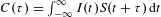 $C(\unicode[STIX]{x1D70F})=\int _{-\infty }^{\infty }I(t)S(t+\unicode[STIX]{x1D70F})\,\text{d}t$
, where
$C(\unicode[STIX]{x1D70F})=\int _{-\infty }^{\infty }I(t)S(t+\unicode[STIX]{x1D70F})\,\text{d}t$
, where
 $\unicode[STIX]{x1D70F}$
is the relative temporal delay between them. The measured cross-correlation function will simply represent the profile of the PT pulse when the sampling pulse has a much higher contrast than the PT pulse. Such a clean sampling pulse is usually generated via second-harmonic generation (SHG) of the replica of PT pulse. This kind of cross-correlation is sometimes called third-order autocorrelation, described equivalently by
$\unicode[STIX]{x1D70F}$
is the relative temporal delay between them. The measured cross-correlation function will simply represent the profile of the PT pulse when the sampling pulse has a much higher contrast than the PT pulse. Such a clean sampling pulse is usually generated via second-harmonic generation (SHG) of the replica of PT pulse. This kind of cross-correlation is sometimes called third-order autocorrelation, described equivalently by
 $A(\unicode[STIX]{x1D70F})=\int _{-\infty }^{\infty }I(t)I^{2}(t+\unicode[STIX]{x1D70F})\,\text{d}t$
.
$A(\unicode[STIX]{x1D70F})=\int _{-\infty }^{\infty }I(t)I^{2}(t+\unicode[STIX]{x1D70F})\,\text{d}t$
.
At present, the DSCC is the workhorse for most contrast measurements[Reference Hong, Hou, Nees, Power and Mourou9–Reference Divall and Ross11]. It gates the PT pulse through instantaneous nonlinear interaction with a clean sampling pulse. The temporal contrast of PT pulse is obtained by recording the cross-correlation signal with variable delay
 $\unicode[STIX]{x1D70F}$
between the interacting pulses [Figure 1(a)]. The delay-scanning configuration allows a highly sensitive photomultiplier (PMT) to detect the cross-correlation signal in sequence, thus a dynamic range of
$\unicode[STIX]{x1D70F}$
between the interacting pulses [Figure 1(a)]. The delay-scanning configuration allows a highly sensitive photomultiplier (PMT) to detect the cross-correlation signal in sequence, thus a dynamic range of
 ${>}10^{10}$
can be achieved. Its measurement temporal window, determined by the range of delay line, can reach hundreds of picoseconds and even up to several nanoseconds. A full measurement often needs a large amount of laser shots.
${>}10^{10}$
can be achieved. Its measurement temporal window, determined by the range of delay line, can reach hundreds of picoseconds and even up to several nanoseconds. A full measurement often needs a large amount of laser shots.

Figure 1. Schematic diagrams of DSCC and three versions of SSCC. (a) DSCC, in which the temporal window is determined by the delay-scanning line. (b) Noncollinear SSCC, in which the PT and sampling pulses are nonlinearly mixed in a noncollinear configuration. Its temporal window is determined by the noncollinear angle and beam width. (c) SSCC based on a pulse replicator, in which a sequence of spatially shifted and temporal delayed sampling pulses are created to nonlinearly mix with the PT pulse. It has a large temporal window of
 ${\sim}200~\text{ps}$
and a temporal resolution of
${\sim}200~\text{ps}$
and a temporal resolution of
 ${\sim}6~\text{ps}$
. (d) SSCC based on a diffraction grating, in which the tilted pulse front of sampling pulse maps the temporal intensity profile of PT pulse into the spatial intensity profile of generated correlation signal. Its temporal window is determined by the tilting angle of sampling pulse front and the beam width. T, PT pulse; S, sampling pulse; C, correlation signal; NC, nonlinear crystal;
${\sim}6~\text{ps}$
. (d) SSCC based on a diffraction grating, in which the tilted pulse front of sampling pulse maps the temporal intensity profile of PT pulse into the spatial intensity profile of generated correlation signal. Its temporal window is determined by the tilting angle of sampling pulse front and the beam width. T, PT pulse; S, sampling pulse; C, correlation signal; NC, nonlinear crystal;
 $\unicode[STIX]{x1D70F}$
, time delay of S relative to T.
$\unicode[STIX]{x1D70F}$
, time delay of S relative to T.
In contrast to DSCC, SSCC performs a full cross-correlation measurement by using a single pulse. Several versions of SSCC have been proposed to create an equivalent range of the delay
 $\unicode[STIX]{x1D70F}$
(i.e., the temporal window), as shown in Figures 1(b)–1(d). A noncollinear interaction configuration between the PT and sampling beams is widely used[Reference Collier, Hernandez-Gomez, Allott, Danson and Hall15–Reference Ginzburg, Didenko, Konyashchenko, Lozhkarev, Luchinin, Lutsenko, Mironov, Khazanov and Yakovlev17]. As shown in Figure 1(b), the noncollinear intersection of the beams on the crystal surface leads to different temporal delays at different transverse locations. In this way, the PT pulse intensity at different time
$\unicode[STIX]{x1D70F}$
(i.e., the temporal window), as shown in Figures 1(b)–1(d). A noncollinear interaction configuration between the PT and sampling beams is widely used[Reference Collier, Hernandez-Gomez, Allott, Danson and Hall15–Reference Ginzburg, Didenko, Konyashchenko, Lozhkarev, Luchinin, Lutsenko, Mironov, Khazanov and Yakovlev17]. As shown in Figure 1(b), the noncollinear intersection of the beams on the crystal surface leads to different temporal delays at different transverse locations. In this way, the PT pulse intensity at different time
 $\unicode[STIX]{x1D70F}$
is encoded into the intensity of correlating signal at different transverse location
$\unicode[STIX]{x1D70F}$
is encoded into the intensity of correlating signal at different transverse location
 $x$
, which is known as the time-to-space encoding. An array detector such as charge-coupled device (CCD) is needed to record the spatial profile of the generated correlation signal. In this configuration, the temporal window of measurement is determined by the intersection angle and beam width. Second-harmonic generation of the PT pulse generates sampling pulse with duration comparable to that of the PT pulse and enhanced contrast as well. Such a sampling pulse duration is acceptable to resolve the noise distribution in a large temporal window that is much larger than the pulse duration. Besides, owing to a large noncollinear angle (
$x$
, which is known as the time-to-space encoding. An array detector such as charge-coupled device (CCD) is needed to record the spatial profile of the generated correlation signal. In this configuration, the temporal window of measurement is determined by the intersection angle and beam width. Second-harmonic generation of the PT pulse generates sampling pulse with duration comparable to that of the PT pulse and enhanced contrast as well. Such a sampling pulse duration is acceptable to resolve the noise distribution in a large temporal window that is much larger than the pulse duration. Besides, owing to a large noncollinear angle (
 ${\sim}40^{\circ }$
) and relatively thin crystal (1–2 mm), the actual temporal resolution in our SSCC is smeared approximately to 1 ps, which is still acceptable in resolving the noise pedestal distributed in a quite large temporal window.
${\sim}40^{\circ }$
) and relatively thin crystal (1–2 mm), the actual temporal resolution in our SSCC is smeared approximately to 1 ps, which is still acceptable in resolving the noise pedestal distributed in a quite large temporal window.
Pulse-front tilting is another configuration that can establish continuously varying time delay based on a single pulse, as shown in Figure 1(d)[Reference Oba, Sun, Mazurenko and Fainman18–Reference Shah, Johnson, Shimada and Hegelich20]. Pulse-front tilting can be realized by using a grating or prism. Similar to Figure 1(b), the time-to-space encoding may be achieved even if the beams are collinear. In principle, both the beam slanting and pulse-front tilting, i.e., the combination of Figures 1(b) and 1(d), can be adopted to further enhance the temporal window of measurement. In addition, the large temporal window in SSCC can also be achieved via a pulse replicator as shown in Figure 1(c)[Reference Dorrer, Bromage and Zuegel21]. It creates variable delays
 $\unicode[STIX]{x1D70F}$
through multiple internal reflections of the sampling pulse in a pulse replicator constituted by a high reflector and a partial reflector. The pulse replicator generates a sequence of temporally delayed and spatially shifted sampling pulses that can be mixed with the PT pulse in a nonlinear crystal. It maps the PT pulse profile, in a discrete manner, into a spatially dispersed one that can be recorded by an array detector. Although it can be favorable in a large temporal window of SSCC, the discrete nature of time-to-space encoding limits the temporal resolution due to the thickness of the replicator.
$\unicode[STIX]{x1D70F}$
through multiple internal reflections of the sampling pulse in a pulse replicator constituted by a high reflector and a partial reflector. The pulse replicator generates a sequence of temporally delayed and spatially shifted sampling pulses that can be mixed with the PT pulse in a nonlinear crystal. It maps the PT pulse profile, in a discrete manner, into a spatially dispersed one that can be recorded by an array detector. Although it can be favorable in a large temporal window of SSCC, the discrete nature of time-to-space encoding limits the temporal resolution due to the thickness of the replicator.
The noncollinear configuration of SSCC shown in Figure 1(b) is more superior in practice due to its simplicity and being easy to use. The correlating signal can be easily picked out due to the noncollinear arrangement. In the following parts, we will focus on this specific configuration and discuss its relevant technologies in detail, including dynamic range, temporal window, temporal resolution and measurement fidelity.
3 Key enabling technologies
3.1 Phase-matching manipulation for large temporal window
Temporal window refers to the achievable delay range between the PT and sampling pulses in an SSCC. In practical applications, a temporal window larger than 50 ps is usually required to match the response limits of a fast photodiode and an oscilloscope, and a temporal resolution of
 ${\sim}1~\text{ps}$
is needed to resolve fine-structured noise. Figure 2(a) shows a typical noncollinear SSCC based on sum-frequency generation (SFG) using a bulk nonlinear crystal. According to its geometrical relations, the temporal window
${\sim}1~\text{ps}$
is needed to resolve fine-structured noise. Figure 2(a) shows a typical noncollinear SSCC based on sum-frequency generation (SFG) using a bulk nonlinear crystal. According to its geometrical relations, the temporal window
 $\unicode[STIX]{x0394}T$
of this SFG-SSCC equals the sum of time delay for the PT pulse through
$\unicode[STIX]{x0394}T$
of this SFG-SSCC equals the sum of time delay for the PT pulse through
 $\overline{BE}$
and that for the sampling pulse through
$\overline{BE}$
and that for the sampling pulse through
 $\overline{AD}$
, which can be calculated by
$\overline{AD}$
, which can be calculated by
 $$\begin{eqnarray}\displaystyle \unicode[STIX]{x0394}T=W/c\cdot (n_{T}\cdot \sin \unicode[STIX]{x1D6FC}+n_{S}\cdot \sin \unicode[STIX]{x1D6FD}), & & \displaystyle\end{eqnarray}$$
where
 $W$
is the transverse width of beam intersection region,
$W$
is the transverse width of beam intersection region,
 $c$
is the light speed in vacuum,
$c$
is the light speed in vacuum,
 $n_{T}\;(n_{S})$
is the refractive index of PT (sampling) pulse and
$n_{T}\;(n_{S})$
is the refractive index of PT (sampling) pulse and
 $\unicode[STIX]{x1D6FC}\;(\unicode[STIX]{x1D6FD})$
is the inner cross-angle between the PT (sampling) and correlation beams. Clearly shown by Equation (1), the temporal window
$\unicode[STIX]{x1D6FC}\;(\unicode[STIX]{x1D6FD})$
is the inner cross-angle between the PT (sampling) and correlation beams. Clearly shown by Equation (1), the temporal window
 $\unicode[STIX]{x0394}T$
is determined by the beam aperture and noncollinear angle. As
$\unicode[STIX]{x0394}T$
is determined by the beam aperture and noncollinear angle. As
 $W$
is ultimately limited by the available crystal aperture, further enhancement of temporal window depends on the increase of angles
$W$
is ultimately limited by the available crystal aperture, further enhancement of temporal window depends on the increase of angles
 $\unicode[STIX]{x1D6FC}$
and
$\unicode[STIX]{x1D6FC}$
and
 $\unicode[STIX]{x1D6FD}$
. However, the angles
$\unicode[STIX]{x1D6FD}$
. However, the angles
 $\unicode[STIX]{x1D6FC}$
and
$\unicode[STIX]{x1D6FC}$
and
 $\unicode[STIX]{x1D6FD}$
are connected to the phase-matching (PM) condition. An efficient SFG requires the phase mismatch,
$\unicode[STIX]{x1D6FD}$
are connected to the phase-matching (PM) condition. An efficient SFG requires the phase mismatch,
 $\unicode[STIX]{x0394}\unicode[STIX]{x1D711}=\unicode[STIX]{x0394}\boldsymbol{k}\boldsymbol{\cdot }\boldsymbol{r}$
, to be minimized. The corresponding wave-vector mismatch is given by
$\unicode[STIX]{x0394}\unicode[STIX]{x1D711}=\unicode[STIX]{x0394}\boldsymbol{k}\boldsymbol{\cdot }\boldsymbol{r}$
, to be minimized. The corresponding wave-vector mismatch is given by
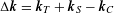 $\unicode[STIX]{x0394}\boldsymbol{k}=\boldsymbol{k}_{T}+\boldsymbol{k}_{S}-\boldsymbol{k}_{C}$
, where
$\unicode[STIX]{x0394}\boldsymbol{k}=\boldsymbol{k}_{T}+\boldsymbol{k}_{S}-\boldsymbol{k}_{C}$
, where
 $\boldsymbol{k}_{T}$
,
$\boldsymbol{k}_{T}$
,
 $\boldsymbol{k}_{S}$
and
$\boldsymbol{k}_{S}$
and
 $\boldsymbol{k}_{C}$
are the wave vectors of the PT, sampling, and correlation pulses, respectively.
$\boldsymbol{k}_{C}$
are the wave vectors of the PT, sampling, and correlation pulses, respectively.
 $\unicode[STIX]{x0394}\boldsymbol{k}$
can be decomposed into parallel and perpendicular components relative to the direction of
$\unicode[STIX]{x0394}\boldsymbol{k}$
can be decomposed into parallel and perpendicular components relative to the direction of
 $\boldsymbol{k}_{C}$
:
$\boldsymbol{k}_{C}$
:
 $\unicode[STIX]{x0394}k_{\Vert }=k_{T}\cos \unicode[STIX]{x1D6FC}+k_{S}\cos \unicode[STIX]{x1D6FD}-k_{C}$
,
$\unicode[STIX]{x0394}k_{\Vert }=k_{T}\cos \unicode[STIX]{x1D6FC}+k_{S}\cos \unicode[STIX]{x1D6FD}-k_{C}$
,
 $\unicode[STIX]{x0394}k_{\bot }=k_{T}\sin \unicode[STIX]{x1D6FC}-k_{S}\sin \unicode[STIX]{x1D6FD}$
. Obviously, owing to the PM condition requirement (
$\unicode[STIX]{x0394}k_{\bot }=k_{T}\sin \unicode[STIX]{x1D6FC}-k_{S}\sin \unicode[STIX]{x1D6FD}$
. Obviously, owing to the PM condition requirement (
 $\unicode[STIX]{x0394}k_{\Vert }=0$
and
$\unicode[STIX]{x0394}k_{\Vert }=0$
and
 $\unicode[STIX]{x0394}k_{\bot }=0$
),
$\unicode[STIX]{x0394}k_{\bot }=0$
),
 $\unicode[STIX]{x1D6FC}$
and
$\unicode[STIX]{x1D6FC}$
and
 $\unicode[STIX]{x1D6FD}$
cannot be set arbitrarily.
$\unicode[STIX]{x1D6FD}$
cannot be set arbitrarily.

Figure 2. PM manipulation and crystal design for noncollinear SSCC. (a) SFG cross-correlation with wide slanting interaction beams.
 $\unicode[STIX]{x1D6FC}\;(\unicode[STIX]{x1D6FD})$
, intersection angle between T (S) and C within NC;
$\unicode[STIX]{x1D6FC}\;(\unicode[STIX]{x1D6FD})$
, intersection angle between T (S) and C within NC;
 $W$
, transverse width of intersecting region between T and S;
$W$
, transverse width of intersecting region between T and S;
 $L$
, longitudinal length of NC. (b) Plot for the analysis of temporal resolution.
$L$
, longitudinal length of NC. (b) Plot for the analysis of temporal resolution.
 $\boldsymbol{k}_{T},\boldsymbol{k}_{S}$
and
$\boldsymbol{k}_{T},\boldsymbol{k}_{S}$
and
 $\boldsymbol{k}_{C}$
are the wave vectors of T, S and C. (c) QPM design in a PPLN crystal with a poling period of
$\boldsymbol{k}_{C}$
are the wave vectors of T, S and C. (c) QPM design in a PPLN crystal with a poling period of
 $\unicode[STIX]{x1D6EC}$
.
$\unicode[STIX]{x1D6EC}$
.
 $\boldsymbol{k}_{\unicode[STIX]{x1D6EC}}$
, the grating
$\boldsymbol{k}_{\unicode[STIX]{x1D6EC}}$
, the grating
 $k$
-vectors provided by PPLN. (d) Lateral cross-correlation supported by high-order QPM.
$k$
-vectors provided by PPLN. (d) Lateral cross-correlation supported by high-order QPM.
 $\unicode[STIX]{x1D70E}$
, beam diameter of S. Its temporal window is limited by the width of PPLN crystal, while its temporal resolution is limited by the beam size
$\unicode[STIX]{x1D70E}$
, beam diameter of S. Its temporal window is limited by the width of PPLN crystal, while its temporal resolution is limited by the beam size
 $\unicode[STIX]{x1D70E}$
.
$\unicode[STIX]{x1D70E}$
.
To mitigate the angle limitation in noncollinear PM, we introduce additional control degrees of freedom. First, the wavelength of sampling pulse can be chosen on demand. We have theoretically and experimentally verified that the increase of sampling wavelength can support larger noncollinear angle and hence larger temporal window[Reference Ma, Yuan, Wang, Zhang, Zhu and Qian26, Reference Qian, Ma, Yuan, Wang, Zhang and Zhu27], as shown in Figure 3(a). Either an optical parametric amplifier (OPA) or a supercontinuum generation (SCG) process, pumped by the replica of PT pulse, can be adopted to generate the required clean long-wavelength sampling pulse[Reference Ma, Yuan, Wang, Zhu and Qian38, Reference Filip, Tóth and Leemans39]. Compared to the conventional short-wavelength SHG sampling, the long-wavelength sampling can increase the wavelength of correlation signal as well, which can better match the spectral range of the low loss and high sensitivity of the fiber-based detection system (see Section 3.2).

Figure 3. (a) Calculated maximum noncollinear angle of SFG (dashed curve) and temporal window (solid curve) with a dependence of sampling wavelength in bulk
 $\text{LiNbO}_{3}$
(black curves) and PPLN (red curves) crystals, respectively, for the SSCC configuration shown in Figure 2(a). (b) Calculated noncollinear angle (dashed curve) and temporal window (solid curve) on the poling period of PPLN for the SSCC configuration in Figure 2(d). Black (red) curves, the first (third)-order QPM. Cross-correlation trace when the width of the narrow sampling beam is set to be (c)
$\text{LiNbO}_{3}$
(black curves) and PPLN (red curves) crystals, respectively, for the SSCC configuration shown in Figure 2(a). (b) Calculated noncollinear angle (dashed curve) and temporal window (solid curve) on the poling period of PPLN for the SSCC configuration in Figure 2(d). Black (red) curves, the first (third)-order QPM. Cross-correlation trace when the width of the narrow sampling beam is set to be (c)
 $150~\unicode[STIX]{x03BC}\text{m}$
and (d)
$150~\unicode[STIX]{x03BC}\text{m}$
and (d)
 $70~\unicode[STIX]{x03BC}\text{m}$
. Inset is the corresponding CCD image of correlation signal. The PT pulse is the output of a 50-fs Ti:sapphire regenerative amplifier.
$70~\unicode[STIX]{x03BC}\text{m}$
. Inset is the corresponding CCD image of correlation signal. The PT pulse is the output of a 50-fs Ti:sapphire regenerative amplifier.
Besides, we may employ quasi-phase matching (QPM) instead of birefringent PM to further release the angle limitation [Figure 2(c)]. QPM, relying on a periodically poled crystal design, can introduce a grating
 $k$
-vector to the PM condition,
$k$
-vector to the PM condition,
 $k_{\unicode[STIX]{x1D6EC}}=2\unicode[STIX]{x1D70B}m/\unicode[STIX]{x1D6EC}$
, where
$k_{\unicode[STIX]{x1D6EC}}=2\unicode[STIX]{x1D70B}m/\unicode[STIX]{x1D6EC}$
, where
 $\unicode[STIX]{x1D6EC}$
is the poling period and
$\unicode[STIX]{x1D6EC}$
is the poling period and
 $m$
is the QPM order. In this case, the parallel component of wave-vector mismatch becomes
$m$
is the QPM order. In this case, the parallel component of wave-vector mismatch becomes
 $\unicode[STIX]{x0394}k_{\Vert }=k_{T}\cos \unicode[STIX]{x1D6FC}\,+\,k_{S}\cos \unicode[STIX]{x1D6FD}-k_{C}-2\unicode[STIX]{x1D70B}m/\unicode[STIX]{x1D6EC}$
. As a result, the PM condition can be manipulated by the two additional parameters of
$\unicode[STIX]{x0394}k_{\Vert }=k_{T}\cos \unicode[STIX]{x1D6FC}\,+\,k_{S}\cos \unicode[STIX]{x1D6FD}-k_{C}-2\unicode[STIX]{x1D70B}m/\unicode[STIX]{x1D6EC}$
. As a result, the PM condition can be manipulated by the two additional parameters of
 $m$
and
$m$
and
 $\unicode[STIX]{x1D6EC}$
. Generally, a shorter period
$\unicode[STIX]{x1D6EC}$
. Generally, a shorter period
 $\unicode[STIX]{x1D6EC}$
and/or a larger order
$\unicode[STIX]{x1D6EC}$
and/or a larger order
 $m$
(only odd integer is valid) leads to a larger temporal window [see Figure 3(b)]. By using a periodically poled lithium niobate (PPLN) crystal with
$m$
(only odd integer is valid) leads to a larger temporal window [see Figure 3(b)]. By using a periodically poled lithium niobate (PPLN) crystal with
 $\unicode[STIX]{x1D6EC}=6~\unicode[STIX]{x03BC}\text{m}$
and
$\unicode[STIX]{x1D6EC}=6~\unicode[STIX]{x03BC}\text{m}$
and
 $m=1$
, for example, we achieved a temporal window per unit
$m=1$
, for example, we achieved a temporal window per unit
 $W$
of
$W$
of
 ${\sim}45~\text{ps}/\text{cm}$
for the SSCC with a sampling wavelength of
${\sim}45~\text{ps}/\text{cm}$
for the SSCC with a sampling wavelength of
 $3.3~\unicode[STIX]{x03BC}\text{m}$
[Reference Ma, Yuan, Wang, Zhang, Zhu and Qian26]. A larger temporal window of
$3.3~\unicode[STIX]{x03BC}\text{m}$
[Reference Ma, Yuan, Wang, Zhang, Zhu and Qian26]. A larger temporal window of
 ${\sim}70~\text{ps}/\text{cm}$
was achieved by using a high-order QPM (e.g.,
${\sim}70~\text{ps}/\text{cm}$
was achieved by using a high-order QPM (e.g.,
 $m=3,5$
)[Reference Ma, Wang, Yuan, Xie, Zhu and Qian28]. A unique lateral cross-correlator with
$m=3,5$
)[Reference Ma, Wang, Yuan, Xie, Zhu and Qian28]. A unique lateral cross-correlator with
 $\unicode[STIX]{x1D6FC}+\unicode[STIX]{x1D6FD}=\unicode[STIX]{x1D70B}/2$
can be realized by high-order QPM owing to its strong capability in compensating phase mismatch, as shown in Figure 2(d). In such a lateral cross-correlator, the sampling pulse is allowed to impinge the PPLN crystal from a lateral surface.
$\unicode[STIX]{x1D6FC}+\unicode[STIX]{x1D6FD}=\unicode[STIX]{x1D70B}/2$
can be realized by high-order QPM owing to its strong capability in compensating phase mismatch, as shown in Figure 2(d). In such a lateral cross-correlator, the sampling pulse is allowed to impinge the PPLN crystal from a lateral surface.
Ideal time-to-space encoding requires a one-to-one correspondence between the time delay
 $\unicode[STIX]{x1D70F}$
and the transverse location
$\unicode[STIX]{x1D70F}$
and the transverse location
 $x$
. This relation is strictly satisfied only on the input surface and then messes up inside the crystal. Such an effect of crystal length
$x$
. This relation is strictly satisfied only on the input surface and then messes up inside the crystal. Such an effect of crystal length
 $L$
on the temporal resolution can be understood with the aid of Figure 2(b). Suppose that the PT beam slice
$L$
on the temporal resolution can be understood with the aid of Figure 2(b). Suppose that the PT beam slice
 $\text{T}_{1}$
and sampling beam slice
$\text{T}_{1}$
and sampling beam slice
 $\text{S}_{1}$
arrive at the point
$\text{S}_{1}$
arrive at the point
 $G$
at the same time (i.e.,
$G$
at the same time (i.e.,
 $\unicode[STIX]{x1D70F}=0$
). They will produce the correlation signal at the main peak, which propagates perpendicularly to the crystal rear surface and emits away from the point
$\unicode[STIX]{x1D70F}=0$
). They will produce the correlation signal at the main peak, which propagates perpendicularly to the crystal rear surface and emits away from the point
 $F$
. Ideally, the intensity of beam light
$F$
. Ideally, the intensity of beam light
 $GF$
only corresponds to the correlation signal at
$GF$
only corresponds to the correlation signal at
 $\unicode[STIX]{x1D70F}=0$
. Unfortunately, it also includes the contributions of correlation signals at
$\unicode[STIX]{x1D70F}=0$
. Unfortunately, it also includes the contributions of correlation signals at
 $\unicode[STIX]{x1D70F}\neq 0$
. As shown in Figure 2(b), for example, the correlation signal between beam slices
$\unicode[STIX]{x1D70F}\neq 0$
. As shown in Figure 2(b), for example, the correlation signal between beam slices
 $\text{T}_{2}$
and
$\text{T}_{2}$
and
 $\text{S}_{2}$
also propagates along
$\text{S}_{2}$
also propagates along
 $GF$
. Thus, the maximum time delay difference is determined by the outmost pair of beam slices as
$GF$
. Thus, the maximum time delay difference is determined by the outmost pair of beam slices as
 $$\begin{eqnarray}\displaystyle \unicode[STIX]{x1D6FF}\unicode[STIX]{x1D70F}=L/c\cdot (n_{T}\cdot \cos \unicode[STIX]{x1D6FC}-n_{S}\cdot \cos \unicode[STIX]{x1D6FD}). & & \displaystyle\end{eqnarray}$$
 $\unicode[STIX]{x1D6FF}\unicode[STIX]{x1D70F}$
reveals the time ambiguity in time-to-space encoding, and is defined as the temporal resolution of the correlation process. According to Equation (2), the temporal resolution also depends on the noncollinear angles
$\unicode[STIX]{x1D6FF}\unicode[STIX]{x1D70F}$
reveals the time ambiguity in time-to-space encoding, and is defined as the temporal resolution of the correlation process. According to Equation (2), the temporal resolution also depends on the noncollinear angles
 $\unicode[STIX]{x1D6FC}$
and
$\unicode[STIX]{x1D6FC}$
and
 $\unicode[STIX]{x1D6FD}$
. Numerical calculations demonstrate that the increase of noncollinear angle (aiming for a larger temporal window) will degrade the temporal resolution. Equations (1) and (2) reveal an inherent trade-off between the temporal window and resolution. It should be noted that the unique lateral cross-correlation shown in Figure 2(d) may break this trade-off, as its temporal resolution is determined by the width
$\unicode[STIX]{x1D6FD}$
. Numerical calculations demonstrate that the increase of noncollinear angle (aiming for a larger temporal window) will degrade the temporal resolution. Equations (1) and (2) reveal an inherent trade-off between the temporal window and resolution. It should be noted that the unique lateral cross-correlation shown in Figure 2(d) may break this trade-off, as its temporal resolution is determined by the width
 $\unicode[STIX]{x1D70E}$
of sampling beam rather than the crystal length
$\unicode[STIX]{x1D70E}$
of sampling beam rather than the crystal length
 $L$
[Reference Ma, Wang, Yuan, Xie, Zhu and Qian28], as shown in Figures 3(c) and 3(d). Due to the limited fiber channels
$L$
[Reference Ma, Wang, Yuan, Xie, Zhu and Qian28], as shown in Figures 3(c) and 3(d). Due to the limited fiber channels
 $N$
in the fiber array (see Section 3.2), the sampling temporal resolution is ultimately limited to
$N$
in the fiber array (see Section 3.2), the sampling temporal resolution is ultimately limited to
 $\unicode[STIX]{x0394}T/N$
. So, the relation between
$\unicode[STIX]{x0394}T/N$
. So, the relation between
 $\unicode[STIX]{x0394}T$
and
$\unicode[STIX]{x0394}T$
and
 $\unicode[STIX]{x1D6FF}\unicode[STIX]{x1D70F}$
can be optimized by matching the correlation resolution
$\unicode[STIX]{x1D6FF}\unicode[STIX]{x1D70F}$
can be optimized by matching the correlation resolution
 $\unicode[STIX]{x1D6FF}\unicode[STIX]{x1D70F}$
with the sampling resolution, i.e.,
$\unicode[STIX]{x1D6FF}\unicode[STIX]{x1D70F}$
with the sampling resolution, i.e.,
 $\unicode[STIX]{x1D6FF}\unicode[STIX]{x1D70F}=\unicode[STIX]{x0394}T/N$
.
$\unicode[STIX]{x1D6FF}\unicode[STIX]{x1D70F}=\unicode[STIX]{x0394}T/N$
.

Figure 4. (a) Schematic diagram of high-sensitivity parallel detection system based on fiber array and PMT. Inset shows the widely used CCD-based parallel detection system. NF, neutral filter. (b) System photograph after packaging. (c) A measurement example of pulse contrast with a dynamic range of
 $10^{10}$
. Reference pulses I, II and III on the correlation trace are achieved by multiple Fresnel reflections of the sampling laser within a 1.1-mm-thick BK7 glass plate.
$10^{10}$
. Reference pulses I, II and III on the correlation trace are achieved by multiple Fresnel reflections of the sampling laser within a 1.1-mm-thick BK7 glass plate.
3.2 High-sensitivity parallel detection for high dynamic range
The dynamic range of an SSCC is defined by the ratio between the maximum and minimum detectable intensities. As the upper limit is restricted by the laser damage of optical elements and thus is fixed to some extent, the dynamic range is mainly limited by the sensitivity of detector used in SSCC. The time-to-space encoding in SSCC precludes the use of single-element PMT detector and necessitates a multi-element detector. The CCD, as a commercial multi-element detector, is extensively used in the majority of SSCC investigations[Reference Collier, Hernandez-Gomez, Allott, Danson and Hall15–Reference He, Zhu, Wang, Cheng, Zou, Wu and Xie23]. However, it has a much poorer sensitivity compared to the known most sensitive PMT detector. As a result, it limits the typical dynamic range of SSCC to about
 $10^{6}$
, much lower than the dynamic range of
$10^{6}$
, much lower than the dynamic range of
 ${>}10^{10}$
obtainable by DSCC with a PMT detector.
${>}10^{10}$
obtainable by DSCC with a PMT detector.
In order to apply sensitive PMT into the SSCC, we proposed and demonstrated an ‘adapter’ that can convert the spatially parallel signal into temporally serial signal[Reference Zhang, Qian, Yuan, Zhu, Wen and Xu29, Reference Qian, Zhang, Yuan and Zhu30]. The adapter to PMT is constituted by 100 fiber channels with different lengths, as shown in Figure 4(a). These fibers are integrated together into a one-dimensional (1D) fiber array by a high precision V-groove technique at one end, and bundled at the other end. The spatially parallel signal will be first sampled by the fiber array into 100 channels of sub-signals. Due to the length increment between adjacent fibers, each sub-signal will be delayed sequentially, thus delivered successively out of the fiber bundle. The time delay (
 $\unicode[STIX]{x0394}t$
) between adjacent sub-signals is determined by the increment of fiber length (
$\unicode[STIX]{x0394}t$
) between adjacent sub-signals is determined by the increment of fiber length (
 $\unicode[STIX]{x0394}l$
) and the refractive index of fiber core (
$\unicode[STIX]{x0394}l$
) and the refractive index of fiber core (
 $n$
),
$n$
),
 $\unicode[STIX]{x0394}t=\unicode[STIX]{x0394}l\cdot n/c$
.
$\unicode[STIX]{x0394}t=\unicode[STIX]{x0394}l\cdot n/c$
.
 $\unicode[STIX]{x0394}t$
should be larger than the response time of PMT to resolve all the 100 sub-signals. For the PMT with a typical response time of 1 ns, the optimal length increment of fiber channels
$\unicode[STIX]{x0394}t$
should be larger than the response time of PMT to resolve all the 100 sub-signals. For the PMT with a typical response time of 1 ns, the optimal length increment of fiber channels
 $\unicode[STIX]{x0394}l$
should be approximately 1–1.5 m.
$\unicode[STIX]{x0394}l$
should be approximately 1–1.5 m.
The invented detection system shown in Figure 4(a) combines a parallel-to-serial mapping of fiber adapter and a high sensitivity of PMT. To accommodate a high dynamic range and ensure a linear response of PMT, a series of variable attenuators may be used to reduce the signal intensities in different fiber channels. Therefore, the fiber-based adapter in practice is often composed of two parts as shown in Figure 4(b). The open ends of these fibers are covered with FC connectors. Normally, the two parts are connected correspondingly with 100 flanges with negligible loss. If needed, fiber attenuators instead of flanges can be used to connect with the corresponding fiber channels. The fiber-based structure used in the detection system facilitates the introduction of variable attenuations for parallel signals. As a comparison, it is more difficult to fabricate the required spatially varying neutral-density filters for CCDs as shown by the inset of Figure 4(a)[Reference Collier, Hernandez-Gomez, Allott, Danson and Hall15–Reference Dorrer, Bromage and Zuegel21]. A band-pass filter at the correlation signal wavelength is added between the fiber bundle and PMT to block the PT and sampling components.
This high-sensitivity parallel detection system promotes the dynamic range of SSCC up to
 $3\times 10^{10}$
, comparable to that of a DSCC, as shown in Figure 4(c)[Reference Wang, Ma, Wang, Yuan, Xie, Ge, Liu, Yuan, Zhu and Qian33]. By inserting a 1.1-mm-thick BK7 plate in the sampling arm, as a demonstration, we can create three equally spaced spikes via multiple Fresnel reflections in the trailing edge of sampling pulse, which will translate into three artificial spikes on the side of correlation trace that corresponds to the leading edge of PT pulse. The evidence for capturing the third replica with a relative intensity of
$3\times 10^{10}$
, comparable to that of a DSCC, as shown in Figure 4(c)[Reference Wang, Ma, Wang, Yuan, Xie, Ge, Liu, Yuan, Zhu and Qian33]. By inserting a 1.1-mm-thick BK7 plate in the sampling arm, as a demonstration, we can create three equally spaced spikes via multiple Fresnel reflections in the trailing edge of sampling pulse, which will translate into three artificial spikes on the side of correlation trace that corresponds to the leading edge of PT pulse. The evidence for capturing the third replica with a relative intensity of
 ${\sim}10^{-9}$
clearly demonstrates the high dynamic range of the SSCC.
${\sim}10^{-9}$
clearly demonstrates the high dynamic range of the SSCC.
3.3 Disturbed noise reduction for high fidelity measurement
The high-sensitivity parallel detection system enhances the detectability for the noise background of PT pulse. On the other hand, it is also sensitive enough to resolve the disturbing or artificial noise produced during the SSCC measurement, such as scattering noise and artificial reflection spikes as illustrated in Figure 5 [Reference Wang, Yuan, Ma and Qian24, Reference Qian, Wang, Yuan, Ma and Xie25]. These disturbing noises may degrade measurement fidelity. It is difficult for a CCD-based SSCC to resolve such measurement noises due to its limited sensitivity. Furthermore, a high dynamic range cannot be practically achieved before the disturbing noise is eliminated or reduced substantially. Note, the disturbing noise such as scattering noise is inherently related to the time-to-space encoding in an SSCC, which does not exist in a conventional DSCC.

Figure 5. Schematic plots for the formation of the SSCC-related artifacts and the methods to remove them. (a) Artificial noise pedestal caused by air scattering of the correlation signal; (b) scattering noise suppression by using a stripe filter. FA, fiber array. SF, stripe filter. (c) The first kind of artificial spikes caused by stray reflection of sampling pulse. (d) A PPLN configuration capable of removing the first kind of artificial spikes. (e) The second kind of artificial spike caused by stray reflection of the correlation signal. (f) Scheme of removing the second kind of artificial spike by controlling the PM condition.
The disturbing noise can be revealed by comparing the correlation trace of SSCC with that of DSCC. Figure 6 summarizes the measurement results of a commercial femtosecond Ti:sapphire regenerative amplifier (details can refer to Ref. [Reference Wang, Yuan, Ma and Qian24]). Typically, an extra pedestal appears on the SSCC trace [black curve in Figure 6(a)], compared to the DSCC trace [red curve in Figure 6(a)]. This pedestal can be attributed to the Rayleigh scattering of the correlation signal by the air gap between the crystal and fiber array, especially by the signal peak [Figure 5(a)]. Owing to the time-to-space encoding, the spatially dispersed scattering background will lead to a pedestal on the correlation trace, even if the PT pulse itself is background-free. The scattering intensity is approximately
 $10^{-8}$
–
$10^{-8}$
–
 $10^{-6}$
of the signal peak[Reference Wang, Ma, Yuan, Tang, Zhou, Xie and Qian40], higher than the system detection limit of
$10^{-6}$
of the signal peak[Reference Wang, Ma, Yuan, Tang, Zhou, Xie and Qian40], higher than the system detection limit of
 $10^{-10}$
. The detection limit may be recovered if we attenuate the signal peak by a factor of at least
$10^{-10}$
. The detection limit may be recovered if we attenuate the signal peak by a factor of at least
 $10^{4}$
. We fabricated a stripe filter that has a transmission of
$10^{4}$
. We fabricated a stripe filter that has a transmission of
 $10^{-4}$
within a 2-mm-wide coating area. Such a stripe filter was placed just behind the crystal with its center aligning to the peak of correlation signal, as shown in Figure 5(b). After dramatic depression of the scattering noise, the true noise pedestal of PT pulse can be well resolved [blue curve in Figure 6(a)].
$10^{-4}$
within a 2-mm-wide coating area. Such a stripe filter was placed just behind the crystal with its center aligning to the peak of correlation signal, as shown in Figure 5(b). After dramatic depression of the scattering noise, the true noise pedestal of PT pulse can be well resolved [blue curve in Figure 6(a)].

Figure 6. Measured correlation traces. (a) Measured SSCC traces before (black curve) and after (blue curve) the elimination of the scattering noise using a stripe filter. Red curve shows the DSCC trace for the same PT pulse as a comparison. The two spikes around
 $+15~\text{ps}$
and
$+15~\text{ps}$
and
 $-15~\text{ps}$
are caused by Fresnel reflections of the PT and sampling pulses between the crystal surfaces. Their intensities are comparable because the crystal refractive indexes at the wavelengths of PT and sampling pulses are nearly the same. (b) SSCC traces measured with the designed PPLN crystal with
$-15~\text{ps}$
are caused by Fresnel reflections of the PT and sampling pulses between the crystal surfaces. Their intensities are comparable because the crystal refractive indexes at the wavelengths of PT and sampling pulses are nearly the same. (b) SSCC traces measured with the designed PPLN crystal with
 $L_{1}=1~\text{mm},L_{2}=2~\text{mm}$
. The black and red curves correspond to the PM conditions of (
$L_{1}=1~\text{mm},L_{2}=2~\text{mm}$
. The black and red curves correspond to the PM conditions of (
 $\unicode[STIX]{x1D6FC}=20^{\circ }$
,
$\unicode[STIX]{x1D6FC}=20^{\circ }$
,
 $\unicode[STIX]{x1D6FD}=44^{\circ }$
) and (
$\unicode[STIX]{x1D6FD}=44^{\circ }$
) and (
 $\unicode[STIX]{x1D6FC}=4^{\circ }$
,
$\unicode[STIX]{x1D6FC}=4^{\circ }$
,
 $\unicode[STIX]{x1D6FD}=78^{\circ }$
), respectively. The red trace has a higher fidelity by removing the two artificial spikes at
$\unicode[STIX]{x1D6FD}=78^{\circ }$
), respectively. The red trace has a higher fidelity by removing the two artificial spikes at
 $-2~\text{ps}$
and
$-2~\text{ps}$
and
 $-4~\text{ps}$
, caused by reflection of correlation signal, to the trailing edge of main pulse.
$-4~\text{ps}$
, caused by reflection of correlation signal, to the trailing edge of main pulse.
As can be seen from Figure 6(a), there are two extra spikes around
 $\pm 15~\text{ps}$
on the SSCC traces compared to the DSCC trace, which can be regarded as measurement artifacts. The artificial spike at the trailing edge of the main pulse is obviously caused by the stray reflection of PT pulse between the crystal surfaces. However, it is hard, at the first sight, to understand the origin of the artificial spike at the leading edge of the main pulse. Actually, it is caused by the stray reflection of sampling pulse between the crystal surfaces [Figure 5(c)]. This type of artificial noise exists in various cross-correlators including DSCCs. Coating the crystal with anti-reflecting film may help reduce this type of artifacts, but can hardly remove them and will degrade the ultrahigh dynamic range. We propose a solution to eliminate this kind of artifacts. As shown in Figure 5(c), the time interval
$\pm 15~\text{ps}$
on the SSCC traces compared to the DSCC trace, which can be regarded as measurement artifacts. The artificial spike at the trailing edge of the main pulse is obviously caused by the stray reflection of PT pulse between the crystal surfaces. However, it is hard, at the first sight, to understand the origin of the artificial spike at the leading edge of the main pulse. Actually, it is caused by the stray reflection of sampling pulse between the crystal surfaces [Figure 5(c)]. This type of artificial noise exists in various cross-correlators including DSCCs. Coating the crystal with anti-reflecting film may help reduce this type of artifacts, but can hardly remove them and will degrade the ultrahigh dynamic range. We propose a solution to eliminate this kind of artifacts. As shown in Figure 5(c), the time interval
 $\unicode[STIX]{x0394}t$
between the first-order artificial spike and the main peak is determined by the crystal length
$\unicode[STIX]{x0394}t$
between the first-order artificial spike and the main peak is determined by the crystal length
 $L$
,
$L$
,
 $\unicode[STIX]{x0394}t=2n_{\text{S}}L/c$
. If
$\unicode[STIX]{x0394}t=2n_{\text{S}}L/c$
. If
 $L$
is large enough to let
$L$
is large enough to let
 $\unicode[STIX]{x0394}t$
be larger than the temporal window
$\unicode[STIX]{x0394}t$
be larger than the temporal window
 $\unicode[STIX]{x0394}T$
, the first-order artificial spike (and also the high-order ones) will move out of the temporal window. However, as implied by Equation (2), the increase of crystal length will degrade the temporal resolution as well. From this point of view, the measurement fidelity and temporal resolution is also a trade-off in SSCC with a bulk crystal. This trade-off can be readily released by the QPM design as shown in Figure 5(d). The crystal can be designed as a combination of a short poled portion (
$\unicode[STIX]{x0394}T$
, the first-order artificial spike (and also the high-order ones) will move out of the temporal window. However, as implied by Equation (2), the increase of crystal length will degrade the temporal resolution as well. From this point of view, the measurement fidelity and temporal resolution is also a trade-off in SSCC with a bulk crystal. This trade-off can be readily released by the QPM design as shown in Figure 5(d). The crystal can be designed as a combination of a short poled portion (
 $L_{1}$
) and a long unpoled portion (
$L_{1}$
) and a long unpoled portion (
 $L_{2}$
). The temporal resolution
$L_{2}$
). The temporal resolution
 $\unicode[STIX]{x1D6FF}\unicode[STIX]{x1D70F}$
is then determined only by the poled portion (
$\unicode[STIX]{x1D6FF}\unicode[STIX]{x1D70F}$
is then determined only by the poled portion (
 $L_{1}$
), whereas the temporal location
$L_{1}$
), whereas the temporal location
 $\unicode[STIX]{x0394}t$
of pre-artifact is determined by the whole crystal length (
$\unicode[STIX]{x0394}t$
of pre-artifact is determined by the whole crystal length (
 $L_{1}+L_{2}$
). Therefore, the pre-artifacts can be tuned far away from the main pulse by increasing
$L_{1}+L_{2}$
). Therefore, the pre-artifacts can be tuned far away from the main pulse by increasing
 $L_{2}$
, whereas a high resolution can be ensured by maintaining a short
$L_{2}$
, whereas a high resolution can be ensured by maintaining a short
 $L_{1}$
[black curve in Figure 6(b)].
$L_{1}$
[black curve in Figure 6(b)].
The increase of whole crystal length makes the SSCC more easily affected by the second kind of artificial spikes, which is caused by stray reflection of correlation signal between the crystal surfaces [see the two spikes just before the main pulse on the black trace shown in Figure 6(b)]. As shown in Figure 5(e), the generated SFG correlation signal is reflected for several times between the crystal surfaces, thus extra spikes will impose on the correlation trace if the SFG beam is not perpendicular to the crystal. The spike locations are determined by the propagation angle of the SFG beam and the length of the crystal. These artificial spikes may immerse in the main peak if the crystal is not long enough. However, in the crystal design shown in Figure 5(d), they can be easily removed owing to the longer crystal. Thanks to the QPM structure, we can shift and delay this kind of artifact far away after the main peak by appropriate parameters setting, as illustrated in Figures 5(f) and 6(b). Thus, proper QPM design may tune both kinds of artifacts out of the temporal window.
4 Instrumentation and applications
4.1 Integration of the key technologies
Here in above, we have introduced several key technologies fulfilling the major demands of a practical SSCC, i.e., high dynamic range, large temporal window, high resolution and high fidelity. A prototype of SSCC is schematically shown in Figure 7(a), which includes three units, i.e., sampling pulse generation, a cross-correlation process and a parallel detection system. The clean sampling pulse can be generated by various nonlinear processes. For example, SHG of the PT pulse can be adopted as a short-wavelength sampling pulse, whereas OPA or SCG process can generate a long-wavelength sampling pulse.

Figure 7. (a) Schematic diagram of noncollinear SSCC. BS, beam splitter;
 $\text{L}_{1}$
, imaging lens;
$\text{L}_{1}$
, imaging lens;
 $\text{L}_{2}$
, focusing lens. (b) SSCC measurement (red curve) versus Sequoia measurement (blue curve). Tiny spikes at
$\text{L}_{2}$
, focusing lens. (b) SSCC measurement (red curve) versus Sequoia measurement (blue curve). Tiny spikes at
 $-27~\text{ps}$
and
$-27~\text{ps}$
and
 $-32~\text{ps}$
, appearing on the red trace were the artifacts caused by the two beam splitters used in SSCC.
$-32~\text{ps}$
, appearing on the red trace were the artifacts caused by the two beam splitters used in SSCC.
The cross-correlation unit undertakes the time-to-space encoding, and determines the main performance of SSCC. Both the PT and sampling beams should be wide enough in the plane (
 $x$
–
$x$
–
 $z$
) of noncollinear PM to support a large temporal window. The beam widths in another transverse dimension (
$z$
) of noncollinear PM to support a large temporal window. The beam widths in another transverse dimension (
 $y$
) can be designed for proper intensities. Both beams in the
$y$
) can be designed for proper intensities. Both beams in the
 $y$
direction should be focused upon the crystal by cylindrical lenses or mirrors. QPM crystals as well as conventional bulk crystals are applicable for the cross-correlation. In a real single-shot environment, bulk crystals may work better than QPM crystals in the aspect of output stability, since QPM crystals typically have a small thickness (e.g., 0.5 mm), which may not overlap with the beams in the
$y$
direction should be focused upon the crystal by cylindrical lenses or mirrors. QPM crystals as well as conventional bulk crystals are applicable for the cross-correlation. In a real single-shot environment, bulk crystals may work better than QPM crystals in the aspect of output stability, since QPM crystals typically have a small thickness (e.g., 0.5 mm), which may not overlap with the beams in the
 $y$
direction. Therefore, the SSCCs developed for PW laser applications adopt the cross-correlation configuration shown in Figure 2(a) with large aperture
$y$
direction. Therefore, the SSCCs developed for PW laser applications adopt the cross-correlation configuration shown in Figure 2(a) with large aperture
 $\unicode[STIX]{x03B2}$
-BBO crystals. The spatial location of the signal pulse peak out of the crystal can be adjusted by the delay line built in the arm of the PT pulse. For revealing the prepulse features, the main peak is often tuned toward the rear edge of the temporal window.
$\unicode[STIX]{x03B2}$
-BBO crystals. The spatial location of the signal pulse peak out of the crystal can be adjusted by the delay line built in the arm of the PT pulse. For revealing the prepulse features, the main peak is often tuned toward the rear edge of the temporal window.
In principle, the noncollinear cross-correlation based on time-to-space encoding requires uniform PT and sampling beams to avoid overestimation of noise. However, the cross-correlation measurement of pulse contrast is very different from the well-known measurement of femtosecond pulse duration. The noise pedestal has fluctuations in the picosecond time scale and also varies orders of magnitude within a large temporal window (
 ${\sim}70~\text{ps}$
in our device). Therefore, the requirement on uniform interacting beams is not so rigid. For instance, typical intensity modulations of diffraction ripples are
${\sim}70~\text{ps}$
in our device). Therefore, the requirement on uniform interacting beams is not so rigid. For instance, typical intensity modulations of diffraction ripples are
 ${\sim}36\%$
at maximum[Reference Siegman41], which may result in
${\sim}36\%$
at maximum[Reference Siegman41], which may result in
 ${\sim}1.36{-}2.5$
times noise overestimation at a specific temporal position, but is still acceptable to the largely varied noise pedestal. It is generally regarded that there is little difference between the high-contrast levels of
${\sim}1.36{-}2.5$
times noise overestimation at a specific temporal position, but is still acceptable to the largely varied noise pedestal. It is generally regarded that there is little difference between the high-contrast levels of
 $1\times 10^{10}$
and
$1\times 10^{10}$
and
 $2.5\times 10^{10}$
, for instance. In addition, the noncollinear cross-correlation is implemented only in the
$2.5\times 10^{10}$
, for instance. In addition, the noncollinear cross-correlation is implemented only in the
 $\mathit{x}$
-dimension, and the beam focusing in the
$\mathit{x}$
-dimension, and the beam focusing in the
 $y$
-dimension can reduce the effect of near-field diffraction and thus the noise overestimation.
$y$
-dimension can reduce the effect of near-field diffraction and thus the noise overestimation.
The generated spatially dispersed correlation signal is collected by the high-sensitivity parallel detection system. To suppress the effect of air scattering on the fidelity, a stripe filter is added just behind the crystal as described in Section 3.3. In the next step, an imaging lens and a focusing lens are used to couple the correlation signal into 100 fibers. A PMT successively converts the 100 optical signals into electrical pulses that can be displayed on a high speed oscilloscope. After data acquisition and calibration, one may retrieve the profile of the PT pulse.
As a demonstration, the SSCC was used to characterize the pulses cleaned by a cross-polarized wave generation (XPW) device. A dynamic range of
 $3\times 10^{10}$
was achieved [Figure 7(b)], which is appropriate for characterizing the pulse contrast of petawatt lasers. Furthermore, we have made a comparison between the measurement results of the SSCC and a commercial DSCC (i.e., Sequoia). The two results show an excellent agreement in terms of the noise background, temporal spikes and the main pulse, as shown in Figure 7(b). The SSCC also successfully measured the pulse contrast of a 200 TW femtosecond Ti:sapphire laser operating at 10 Hz[Reference Wang, Ma, Wang, Yuan, Xie, Ge, Liu, Yuan, Zhu and Qian33].
$3\times 10^{10}$
was achieved [Figure 7(b)], which is appropriate for characterizing the pulse contrast of petawatt lasers. Furthermore, we have made a comparison between the measurement results of the SSCC and a commercial DSCC (i.e., Sequoia). The two results show an excellent agreement in terms of the noise background, temporal spikes and the main pulse, as shown in Figure 7(b). The SSCC also successfully measured the pulse contrast of a 200 TW femtosecond Ti:sapphire laser operating at 10 Hz[Reference Wang, Ma, Wang, Yuan, Xie, Ge, Liu, Yuan, Zhu and Qian33].
4.2 Installation and initialization
In this section, we simply introduce how to install the SSCC in single-shot laser situation, and emphasize on how to quickly set the proper attenuations for achieving high dynamic range. The SSCC employs two types of attenuation. The first type is the stripe filter behind the correlating crystal for suppressing the scattering noise. The second type is the attenuators in the fiber channels for tuning the output signal from fiber bundle within the dynamic range of PMT. In order to ensure linear response, we keep all the sub-signals within a relative range of
 ${\sim}10^{3}$
, although the typical dynamic range of PMT is about
${\sim}10^{3}$
, although the typical dynamic range of PMT is about
 $10^{5}$
. Here, we illustrate the procedure for presetting the two types of attenuation by a virtual example of the PT pulse, as shown in Figure 8(a).
$10^{5}$
. Here, we illustrate the procedure for presetting the two types of attenuation by a virtual example of the PT pulse, as shown in Figure 8(a).

Figure 8. (a) An exemplary PT pulse profile with a strong prepulse and a noise pedestal around the main pulse. (b)–(d) Presetting procedure for the attenuations of SSCC aiming at measuring the PT pulse shown in (a).
As the PT pulse profile is unknown in advance, we first insert a piece of neutral-density filter before the fiber array, whose attenuation should be initially selected to be high enough and be reduced step by step in order to protect the PMT. Suppose such an external filter with a
 $10^{5}$
attenuation is properly set, then one can determine the spatial locations of the main pulse and one prepulse by using the first laser shot of test. As the generated correlation signals, at these two locations, are intense enough to produce scattering noise, both of them should be attenuated by additional stripe filters. Based on the first-shot test measurement, two stripe filters with attenuation of
$10^{5}$
attenuation is properly set, then one can determine the spatial locations of the main pulse and one prepulse by using the first laser shot of test. As the generated correlation signals, at these two locations, are intense enough to produce scattering noise, both of them should be attenuated by additional stripe filters. Based on the first-shot test measurement, two stripe filters with attenuation of
 $10^{6}$
(i.e., over the dynamic range of PMT) and
$10^{6}$
(i.e., over the dynamic range of PMT) and
 $10^{4}$
(i.e., over the relative sub-signal range of
$10^{4}$
(i.e., over the relative sub-signal range of
 $10^{3}$
) are inserted at the spatial locations of the main pulse and the prepulse, respectively. After setting the stripe filters, we lower the attenuation of neutral-density filter from
$10^{3}$
) are inserted at the spatial locations of the main pulse and the prepulse, respectively. After setting the stripe filters, we lower the attenuation of neutral-density filter from
 $10^{5}$
to
$10^{5}$
to
 $10^{2}$
, a reduction factor same to the relative sub-signal range of
$10^{2}$
, a reduction factor same to the relative sub-signal range of
 $10^{3}$
. At this moment, we are ready for the second laser shot of test. For the PT pulse example shown in Figure 8(a), noise pedestal exists around the main pulse, and thus attenuators in the fiber channels are needed. As the external neutral-density filter will be removed away finally, attenuation of
$10^{3}$
. At this moment, we are ready for the second laser shot of test. For the PT pulse example shown in Figure 8(a), noise pedestal exists around the main pulse, and thus attenuators in the fiber channels are needed. As the external neutral-density filter will be removed away finally, attenuation of
 $10^{2}$
at least or higher for the fiber channels around the main pulse is required. We can remove the external neutral filter when the fiber attenuators are well set. Finally, we further check if the sub-signal amplitude in each fiber channel has been adjusted appropriately by a third laser shot of test.
$10^{2}$
at least or higher for the fiber channels around the main pulse is required. We can remove the external neutral filter when the fiber attenuators are well set. Finally, we further check if the sub-signal amplitude in each fiber channel has been adjusted appropriately by a third laser shot of test.
The step-by-step method introduced in Figure 8 allows the complete presetting of attenuations associated in the SSCC only by three laser shots of test, although 100 fiber channels are involved. After this initialization, the SSCC can start working online as a real-time monitor for pulse contrast. At current stage, it needs about twenty minutes to read out and process the 100 sub-signals artificially for each measurement. In next step, we plan to develop a real-time data processor for our SSCC.

Figure 9. Two application examples of the SSCC prototypes. (a) Picture of the 1053-nm version and (b) contrast measurement result for the SG-II Nd:glass petawatt laser. (c) Picture of the 800-nm version and (d) contrast measurement result for the SULF-5 PW Ti:sapphire laser.
4.3 In situ applications on petawatt laser facilities
Until now, we have developed five SSCC prototypes for the petawatt facilities in China with two typical examples shown in Figure 9. These SSCCs include two wavelength versions, the 1053-nm version [Figure 9(a)] and the 800-nm version [Figure 9(c)]. Since the year of 2014, the 1053-nm version has been operating on the SG-II Nd:glass petawatt laser at Shanghai Institute of Optics and Fine Mechanics (SIOM), Chinese Academy of Sciences (CAS)[Reference Ouyang, Cui, Zhu, Zhu and Zhu35]. Four other sets of the 800-nm version have been applied successively on the 1-PW Ti:sapphire laser at SIOM of CAS, the 1-PW Ti:sapphire laser at Institute of Physics (IOP) of CAS, the 5-PW OPCPA laser at Laser Fusion Research Center (LFRC) of China Academy of Engineering Physics (CAEP)[Reference Zeng, Zhou, Zuo, Zhu, Su, Wang, Wang, Huang, Jiang, Jiang, Guo, Xie, Zhou, Wu, Mu, Peng and Jing36] and the 5-PW Ti:sapphire laser at Shanghai Superintense Ultrafast Laser Facility (SULF) of CAS[Reference Yu, Xu, Liu, Li, Li, Liu, Li, Wu, Yang, Yang, Wang, Leng, Li and Xu37]. All these laser facilities operate in a single-shot mode, which are appropriate sources for testing the performance of the SSCCs. All the SSCCs have succeeded in measuring the pulse contrast with a dynamic range of
 $10^{10}$
, with one example shown in Figure 9(d). Besides, the SSCCs can also be used as real-time monitors for the optimization of laser operation. With the aid of the SSCC, pulse contrast of the SG-II PW laser facility has been improved from
$10^{10}$
, with one example shown in Figure 9(d). Besides, the SSCCs can also be used as real-time monitors for the optimization of laser operation. With the aid of the SSCC, pulse contrast of the SG-II PW laser facility has been improved from
 $10^{4}$
initially to
$10^{4}$
initially to
 $10^{8}$
actually [Figure 9(b)], which is the reported highest pulse contrast among the Nd:glass petawatt lasers worldwide[Reference Ouyang, Cui, Zhu, Zhu and Zhu35].
$10^{8}$
actually [Figure 9(b)], which is the reported highest pulse contrast among the Nd:glass petawatt lasers worldwide[Reference Ouyang, Cui, Zhu, Zhu and Zhu35].
In these SSCCs, the large-size
 $\unicode[STIX]{x03B2}$
-BBO crystals are adopted, which may support a temporal window of 50 ps for the 800-nm version and 70 ps for the 1053-nm version, respectively. Extension of temporal window can be realized via splicing several single-shot measurement results, with successive increment of the relative delay by adjusting the delay line built in the arm of PT pulse. The delay increment should be less than the single-shot temporal window, such that the data in the overlapped part of adjacent measurements can be used as calibration base, assuming shot-to-shot fluctuation is negligible. Such a multi-shot measurement scheme can extend the measurement temporal range to
$\unicode[STIX]{x03B2}$
-BBO crystals are adopted, which may support a temporal window of 50 ps for the 800-nm version and 70 ps for the 1053-nm version, respectively. Extension of temporal window can be realized via splicing several single-shot measurement results, with successive increment of the relative delay by adjusting the delay line built in the arm of PT pulse. The delay increment should be less than the single-shot temporal window, such that the data in the overlapped part of adjacent measurements can be used as calibration base, assuming shot-to-shot fluctuation is negligible. Such a multi-shot measurement scheme can extend the measurement temporal range to
 ${>}100~\text{ps}$
, which is limited by the range of the delay line. The results shown in Figures 9(b) and 9(d) are obtained both by using two shots. The successful applications verify the feasibility and practicability of the SSCCs. Besides, it can be easily extended to other laser wavelengths. Actually, the SSCC will show better measurement performance in mid-IR spectral region since the longer wavelength of correlation signal matches the detection system better in this case.
${>}100~\text{ps}$
, which is limited by the range of the delay line. The results shown in Figures 9(b) and 9(d) are obtained both by using two shots. The successful applications verify the feasibility and practicability of the SSCCs. Besides, it can be easily extended to other laser wavelengths. Actually, the SSCC will show better measurement performance in mid-IR spectral region since the longer wavelength of correlation signal matches the detection system better in this case.
5 Discussion and Conclusion
The aim of pulse-contrast measurement is to reveal the noise background and prepulse spikes at the leading edge of the main pulse, and hence to judge whether it is below the ionization threshold of the target. Most current SSCCs characterize laser pulses in the near-field, whereas targets are normally located in the far-field (i.e., at the focus). One question arises: whether the near-field measurement results can correctly reflect the pulse contrast on the target? The answer to this question depends on the spatiotemporal (ST) nature of noise. For noises without ST coupling, such as amplified spontaneous emission and optical parametric superfluorescence, the noise characteristics in the far-field can be well revealed by near-field measurements. However, the noise generated in the pulse stretcher and compressor of a CPA system usually exhibits ST coupling characteristics due to the involved angular dispersion[Reference Bromage, Dorrer and Jungquist42–Reference Li, Miyanaga and Kawanaka44]. The conventional SSCC and DSCC, lack of spatial resolving ability, will not be applicable for measuring such ST noise. Full characterization of ST noise requires two-dimensional (2D) measurements.
For this purpose, the SSCC can be extended from the temporal domain to the ST domain[Reference Ma, Yuan, Wang, Wang, Xie, Zhu and Qian31, Reference Qian, Ma, Yuan, Wang, Wang, Xie and Zhu32], as shown in Figure 10(c). The PT beam is focused in the
 $x$
-dimension, in which the angular dispersions of the stretcher and compressor present, on the surface of nonlinear crystal, whereas the sampling beam remains wide in the
$x$
-dimension, in which the angular dispersions of the stretcher and compressor present, on the surface of nonlinear crystal, whereas the sampling beam remains wide in the
 $x$
-dimension to create variable delays [Figure 10(b)]. In the
$x$
-dimension to create variable delays [Figure 10(b)]. In the
 $y$
-dimension, both the PT and sampling beams are wide, and the conventional noncollinear configuration results in a single-shot temporal window [Figure 10(a)]. The generated 2D correlation pattern is imaged onto the fiber array. Compared to the SSCC shown in Figure 7(a), the imaging system in the STCC has two differences. The imaging lens in the STCC is a spherical lens to realize 2D imaging. Besides, there is no focusing lens before the fiber array for maintaining spatial resolution. If a 1D fiber array is used in the STCC, it should be translated along the
$y$
-dimension, both the PT and sampling beams are wide, and the conventional noncollinear configuration results in a single-shot temporal window [Figure 10(a)]. The generated 2D correlation pattern is imaged onto the fiber array. Compared to the SSCC shown in Figure 7(a), the imaging system in the STCC has two differences. The imaging lens in the STCC is a spherical lens to realize 2D imaging. Besides, there is no focusing lens before the fiber array for maintaining spatial resolution. If a 1D fiber array is used in the STCC, it should be translated along the
 $\unicode[STIX]{x1D703}_{x}$
direction to record the temporal contrast at different
$\unicode[STIX]{x1D703}_{x}$
direction to record the temporal contrast at different
 $\unicode[STIX]{x1D703}_{x}$
. When the fiber array is fixed at
$\unicode[STIX]{x1D703}_{x}$
. When the fiber array is fixed at
 $\unicode[STIX]{x1D703}_{x}=0$
, it can record the far-field on-axis contrast, which is more relevant for high-field experiments[Reference Lu, Wang, Leng, Guo, Peng, Li, Xu, Xu and Qi45]. To realize a complete single-shot STCC, a 2D fiber array should be used to record the 2D correlation image.
$\unicode[STIX]{x1D703}_{x}=0$
, it can record the far-field on-axis contrast, which is more relevant for high-field experiments[Reference Lu, Wang, Leng, Guo, Peng, Li, Xu, Xu and Qi45]. To realize a complete single-shot STCC, a 2D fiber array should be used to record the 2D correlation image.

Figure 10. Schematic diagram of spatiotemporal cross-correlator (STCC).
In conclusion, we have discussed the recent progress of SSCCs developed by our group. We have improved the measurement performance based on the key technologies, such as PM manipulation by QPM, high-sensitivity parallel detection scheme based on fiber array and PMT and suppression of disturbed noises during the measurement. By integrating these techniques, we have developed several SSCC prototypes, which have been successfully applied in five sets of petawatt laser facilities in China. These SSCCs not only measure but also help improve the pulse contrast of laser facilities. Our SSCC devices with a high dynamic range of
 $10^{10}$
have already satisfied the requirement of current petawatt lasers, and higher dynamic range of
$10^{10}$
have already satisfied the requirement of current petawatt lasers, and higher dynamic range of
 ${\sim}10^{12}$
is currently under investigation for future 100-PW lasers. The next SSCC version will consist of two cross-correlators that may separately characterize the main pulse in a small window (10 ps) and the noise pedestal in a large window (100 ps), so that a higher temporal resolution (100 fs) for the main pulse can be anticipated. Besides, a high dynamic range of
${\sim}10^{12}$
is currently under investigation for future 100-PW lasers. The next SSCC version will consist of two cross-correlators that may separately characterize the main pulse in a small window (10 ps) and the noise pedestal in a large window (100 ps), so that a higher temporal resolution (100 fs) for the main pulse can be anticipated. Besides, a high dynamic range of
 $10^{12}$
might be possible based on the combination of higher sensitivity PMT and low-noise electrical amplifier.
$10^{12}$
might be possible based on the combination of higher sensitivity PMT and low-noise electrical amplifier.
Acknowledgements
This work was partially supported by the National Natural Science Foundation of China (NSFC) (Nos. 61705128, 61727820, and 91850203), Shanghai Sailing Program (No. 17YF1409100), and Natural Science Foundation of Shanghai (No. 17ZR1414000). We appreciate Dongfang Zhang for his early contributions to the parallel detection system, Yongzhi Wang for the noise reduction methods and high dynamic measurement, Xiaoping Ouyang for providing the measurement data of Figure 9(b), and Yi Xu for providing the measurement data of Figure 9(d). We also acknowledge the institutions of SIOM, IOP and LFRC for their applications of our SSCCs.


 Open access