


1. Introduction
Laser-driven inertial fusion energy is one of the most promising approaches for the sustainable generation of electrical power. Research on laser-driven inertial confinement fusion (ICF) has resulted in the world’s largest laser systems, such as NIF and LMJ [Reference Haynam, Wegner, Auerbach, Bowers, Dixit, Erbert, Heestand, Henesian, Hermann, Jancaitis, Manes, Marshall, Mehta, Menapace, Moses, Murray, Nostrand, Orth, Patterson, Sacks, Shaw, Spaeth, Sutton, Williams, Widmayer, White, Yang and Van Wonterghem1, Reference Ebrardt and Chaput2]. While single-shot facilities can be used to study the basic physics and technology of laser fusion, they are not applicable for the continuously operated power plants of the future. Recent studies have shown that diode-pumped solid-state lasers (DPSSLs) are the most promising laser systems to reach the requirements for such a driver, namely multi-100 kJ energy of ns pulses, multi-Hz repetition rates and high wall-plug efficiencies between 10% and 15%[Reference Chanteloup, Albach, Lucianetti, Ertel, Banerjee, Mason, Hernandez-Gomez, Collier, Hein, Wolf, Körner and Garrec3, Reference Erlandson, Aceves, Bayramian, Bullington, Beach, Boley, Caird, Deri, Dunne, Flowers, Henesian, Manes, Moses, Rana, Schaffers, Spaeth, Stolz and Telford4]. The HiLASE team is developing an  ${\mathrm{Yb}}^{{3+}}$:YAG gain medium based concept for a $100\ {\rm J}/10\ {\rm Hz}$ DPSSL amplifier that could potentially be scaled to the kJ regime[Reference Sawicka, Divoky, Novak, Lucianetti, Rus and Mocek5–Reference Slezak, Lucianetti, Divoky, Sawicka and Mocek7]. While there are several projects around the world that are trying to achieve the same goal[Reference Novo, Albach, Vincent, Arzakantsyan and Chanteloup8–Reference Hein, Kaluza, Bodefeld, Siebold, Podleska, Sauerbrey, Schwoerer, Magill and Beleites11], HiLASE is expected to be completed in May 2015 and it will be the world’s highest pulse energy short pulse (2–10 ns) DPSSL at 100 J and 1–10 Hz.
In this paper, we examine the predicted performance of a kJ-class HiLASE laser which is based on a gas-cooled slab-stack architecture. It uses multiple thin slabs of  ${\mathrm{Yb}}^{{3+}}$:YAG gain medium, face-cooled with high-pressure streaming helium gas[Reference Divoky, Sikocinski, Pilar, Lucianetti, Sawicka, Slezak and Mocek12, Reference Ertel, Banerjee, Mason, Phillips, Siebold, Hernandez-Gomez and Collier13]. The goal of this paper is to provide an amplifier design for the kJ-class laser architecture that minimizes accumulated nonlinear phase (B integral), thermally induced wavefront aberrations and stress birefringence. In Section 2, we describe our model for the calculation of output energy. In Section 3, we describe the HiLASE laser concept and show calculations performed using our energetics modeling. In Section 4, we present the results from the MIRO model used to determine the temporal profile of the output beam and the evolution of the amplified beam as it propagates through the optical system. In Section 5, we show thermal modeling results, including optimization of optical path difference (OPD) and thermally induced stress birefringence. In Section 6, we present the optimized structure parameters of deformable mirrors (DMs) for wavefront correction. Finally, we present our modeling results for frequency conversion in Section 7.
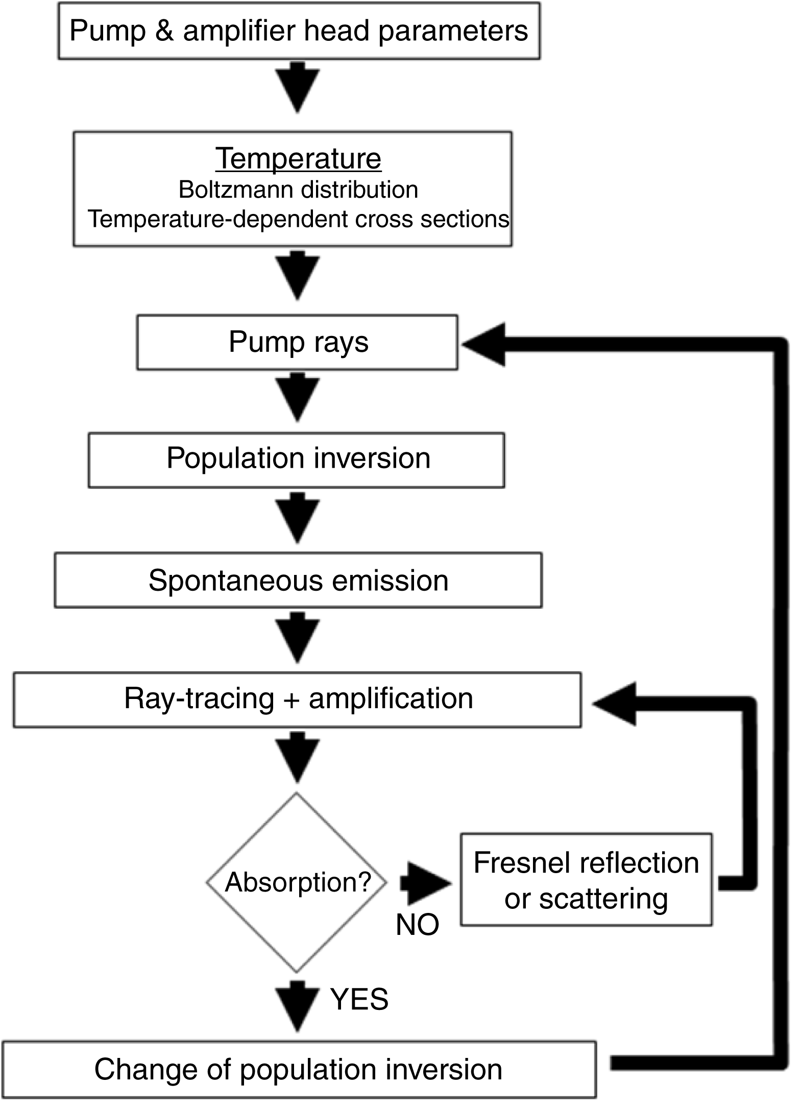
Figure 1. A schematic flow diagram of the model.
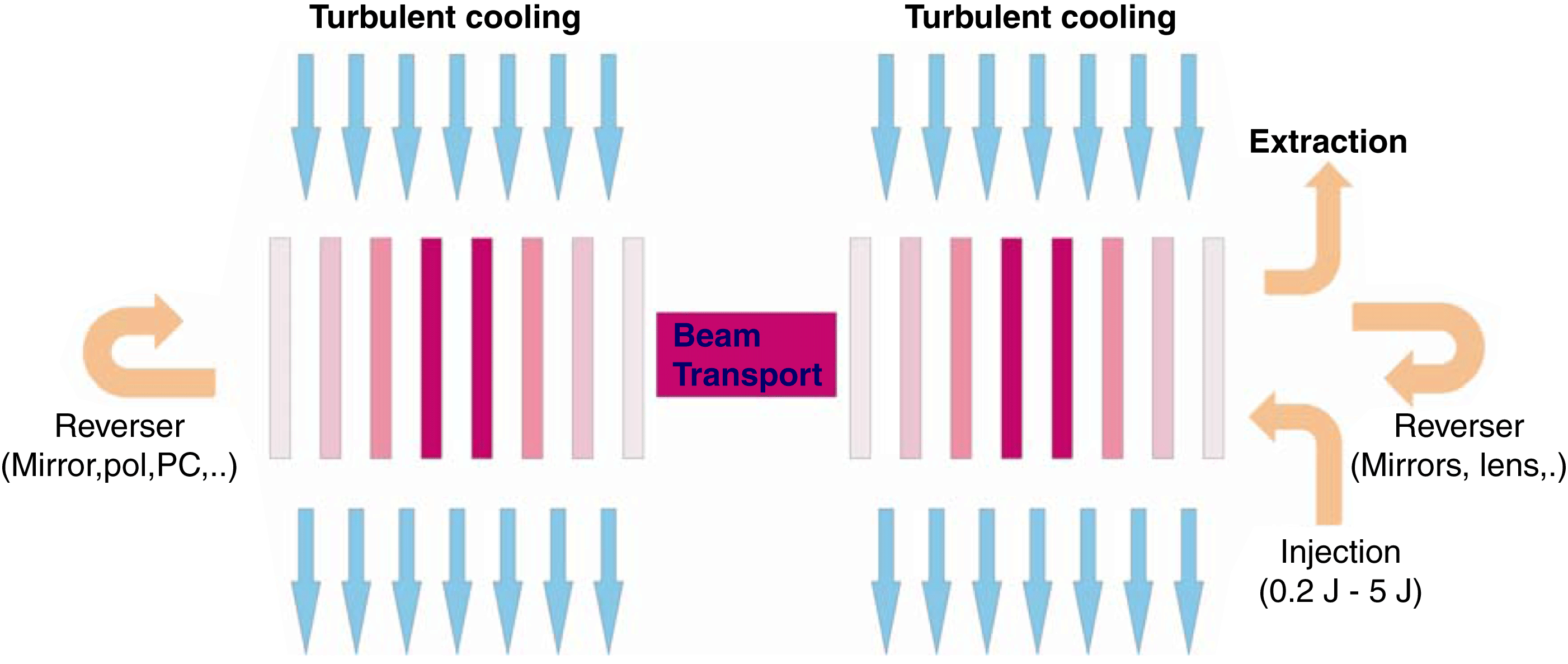
Figure 2. Block diagram of the HiLASE kJ laser (two-head configuration).
2. Energetics modeling
To quantitatively assess energy storage and amplified spontaneous emission (ASE) losses within the laser active material in multi-slab geometry, a numerical model has been developed[Reference Sawicka, Divoky, Novak, Lucianetti, Rus and Mocek5]. Figure 1 shows a flow chart of the code. At the beginning, the parameters of the amplifier head are specified including the temperature of operation. The population of each laser level is calculated from the Boltzmann distribution. For a given temperature, wavelength-dependent emission and absorption cross sections are uploaded from the database. Each slab is divided into pixels, which contain information about the total number of active ions. The information about the excited fraction of ions is also stored in the memory. The slabs will absorb polychromatic pump radiation proportionally to the number of non-excited active ions and the wavelength resolved absorption cross-section.
Based on the excited ion density, the spontaneously emitted photons are generated in the form of rays. Each ray is traced through the slab and the number of photons is changed after the ray undergoes amplification or absorption. At the same time, the excited ion density in appropriate cells is also recalculated. Photons that are not absorbed in the cladding propagate up to the side edge of the slab. The probability of reflection at the edge is calculated from the Fresnel equations for the incident angle of the ray. If photons are reflected back, they pass through the absorptive layer again and, if they are not absorbed, they propagate back to the gain medium and decrease the stored energy[Reference Sawicka, Divoky, Lucianetti and Mocek6].
3. Amplifier concept and simulations
For our kJ-class HiLASE laser, we have chosen to model an amplifier with the characteristics derived from the previous ASE and thermal study[Reference Sawicka, Divoky, Lucianetti and Mocek6, Reference Slezak, Lucianetti, Divoky, Sawicka and Mocek7], i.e., eight 1 cm thick  ${\mathrm{Yb}}^{{3+}}$:YAG slabs with transverse dimensions of 14 cm $\times $ 14 cm. A 2 cm wide ${\mathrm{Cr}}^{\mathrm{4+}}$:YAG absorptive cladding ( $a=1.1\ {\mathrm{cm}}^{-1}$ at 1030 nm) around the edge of each slab was also included to further suppress ASE and prevent unwanted parasitic oscillations. The edges of the cladding were modeled as roughened surfaces which scatter rays. The optimized doping concentrations for the eight-slab amplifier were 0.29, 0.38, 0.56, and 0.85 at.%. The super-Gaussian pump dimensions were kept at 14 cm $\times $ 14 cm which corresponded to a total pump area of 196 ${\rm cm}^{2}$. The operating temperature was allowed to vary between 160 and 240 K. Two different beamline concepts are considered here. In the first concept, the output from a low-energy preamplifier (0.2–5 J) is sent to the main kJ amplifier consisting of two identical heads (Figure 2).
In the second design, the laser beam is preamplified up to a 100 J level and then sent to a single kJ laser head (Figure 3).

Figure 3. Block diagram of the HiLASE kJ laser (single-head configuration).
To find out how the energy is stored in the amplifier, a time-resolved calculation was conducted. In this case, the two-head design was considered. Figures 4–6 show the extractable energy as a function of time for different pump intensities at temperatures of 160, 200, and 240 K.
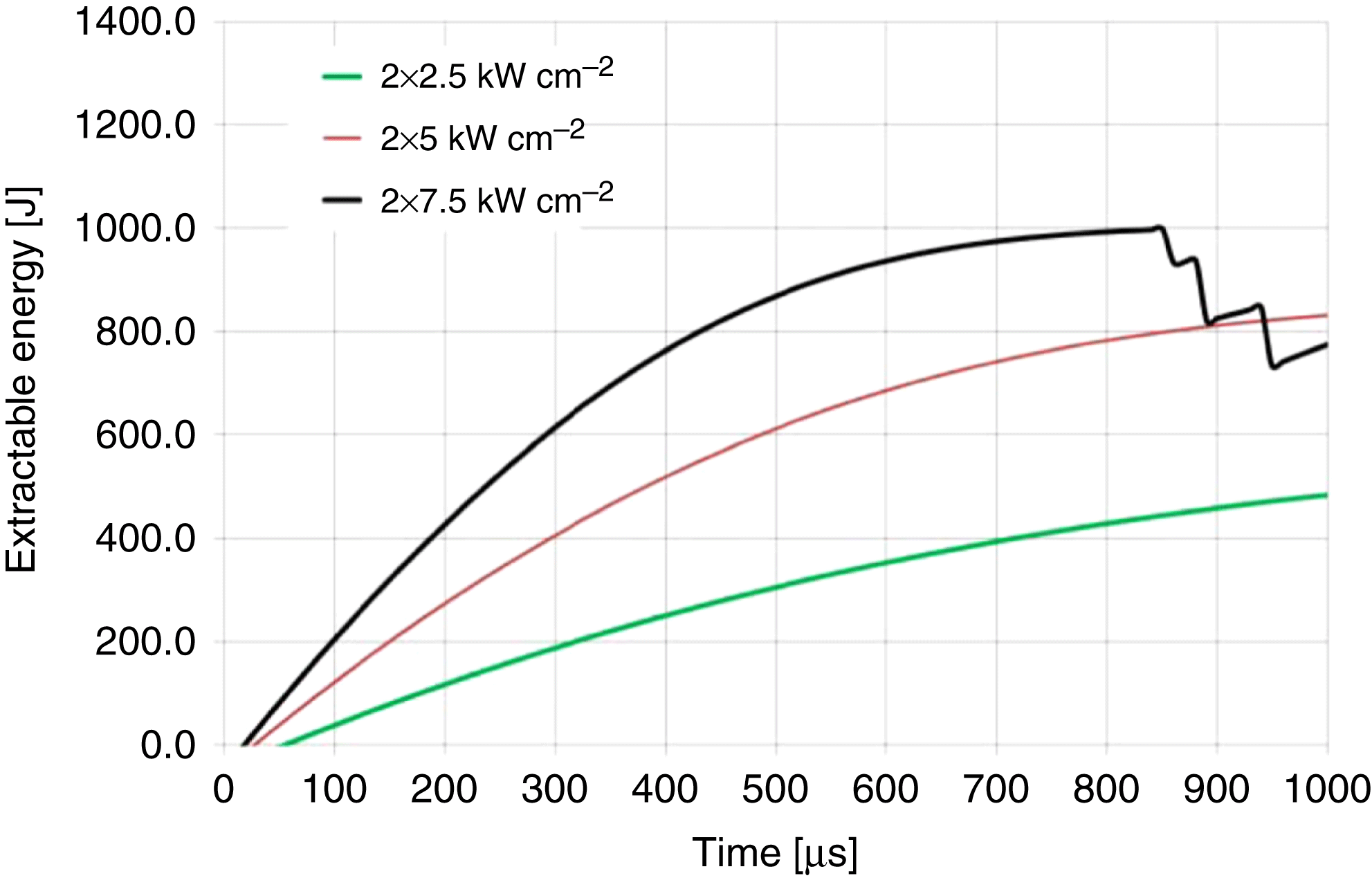
Figure 4. The time-resolved extractable energy in the HiLASE slab for different pump intensities ( $T = 160$ K).
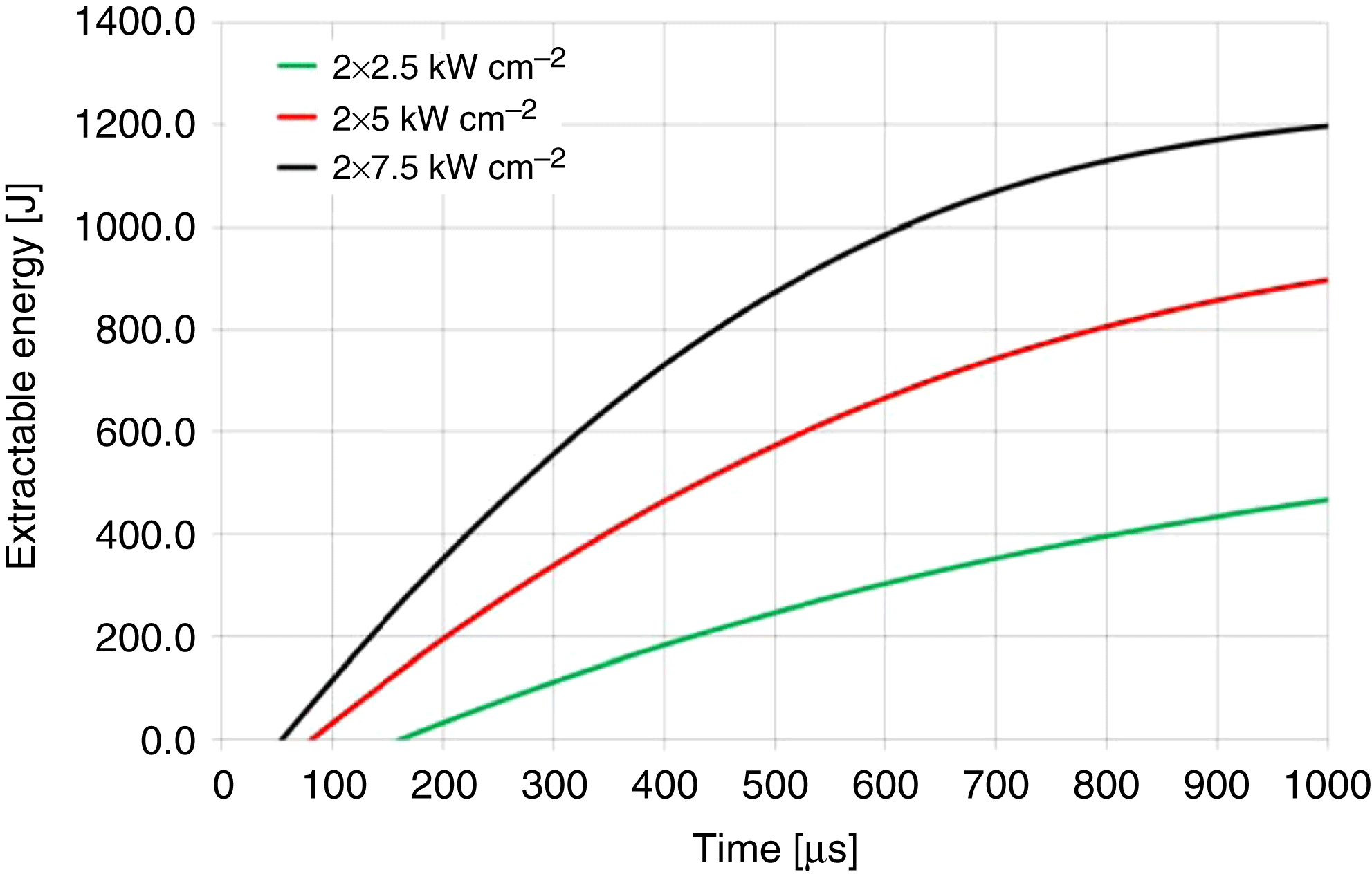
Figure 5. The time-resolved extractable energy in the HiLASE slab for different pump intensities ( $T = 200$ K).
Large values of the ASE saturate the gain and the pump duration of 1 ms is too long for effective energy storage at low temperatures (see Figure 4). It is noted that an extractable energy of more than 1 kJ can be obtained for pump durations of 1 ms and temperatures greater than 200 K. In addition, there is an optimal temperature for which the extractable energy is the highest. For higher pump intensities, the excitation of the gain medium is higher and the temperature-dependent emission cross section plays a significant role. If the temperature is increasing, the emission cross section of the Yb:YAG is decreasing and therefore the ASE losses are also decreasing. Therefore, the optimal temperature is shifting towards higher temperatures with increasing pump intensity. The extractable energy is the stored energy minus the energy bound to the lower laser level due to the three-level nature of the  ${\mathrm{Yb}}^{{3+}}$:YAG (energy needed for the gain medium to stay transparent). The extractable energy as a function of temperature was calculated for different pump intensities for a single amplifier head (Figure 7).

Figure 6. The time-resolved extractable energy in the HiLASE slab for different pump intensities ( $T = 240$ K).

Figure 7. The extractable energy as a function of the operating temperature for different pump intensities.
The storage efficiency was calculated as the ratio between the absorbed energy and the extractable energy (Figure 8). Higher pump intensity causes higher ASE losses. Therefore, at lower temperatures the storage efficiency decreases with increase of pump intensity.

Figure 8. The storage efficiency as a function of the operating temperature for different pump intensities.
Based on the previous results, an operating temperature of 200 K and a pump duration of 1 ms were selected. The following figures give an indication of the evolution of the energy generated after each pass through the pair of amplifiers (Figures 9 and 10) or single amplifier (Figures 11 and 12) at 200 K.

Figure 9. The evolution of the extracted energy for different input energies at 200 K (two heads, 20% optical losses per round trip pass). The total pump intensity was  $2 \times 10\ {\rm kW}\ {\rm cm}^{-2}$.

Figure 10. The evolution of the extracted energy for different input energies at 200 K (two heads, 16% optical losses per round trip pass). The total pump intensity was  $2 \times 10\ {\rm kW}\ {\rm cm}^{-2}$.

Figure 11. The evolution of the extracted energy for different input energies at 200 K (one head, 18% optical losses per round trip pass). The total pump intensity was  $15\ {\rm kW}\ {\rm cm}^{-2}$.

Figure 12. The evolution of the extracted energy for different input energies at 200 K (one head, 10% optical losses per round trip pass). The total pump intensity was  $15\ {\rm kW}\ {\rm cm}^{-2}$.
It is noted that an output energy of 0.92 kJ can be reached in the single-head design with reasonably low values of optical losses (10%) and an operating temperature of 200 K. In this case, the input beam can be provided by next-generation high-energy-class (HEC)-DPSSL facilities with output energies in the range of 100–150 J[Reference Novo, Albach, Vincent, Arzakantsyan and Chanteloup8, Reference Divoky, Sikocinski, Pilar, Lucianetti, Sawicka, Slezak and Mocek12, Reference Ertel, Banerjee, Mason, Phillips, Siebold, Hernandez-Gomez and Collier13].

Figure 13. The MIRO model used to calculate the temporal shape, spatial shape, and B integral of the HiLASE kJ laser.
4. Beam propagation
In order to carry out fundamental calculations on how a HiLASE kJ laser would operate, a MIRO model has been constructed for the two-head configuration. These calculations are based on previous modeling results for the two-head design for a 100 J-class HiLASE amplifier[Reference Divoky, Sikocinski, Pilar, Lucianetti, Sawicka, Slezak and Mocek12]. We assumed that all surfaces are anti-reflection coated with a reflectivity of 0.5%, and all optical elements are made of appropriate material, i.e., fused silica ( $n_{2}=3e^{-20}\ \mathrm{m}^{2}\ \mathrm{W}^{-1}$) for the lenses and windows of the spatial filters, DKDP ( $n_{2}=10e^{-20}\ \mathrm{m}^{2}\ \mathrm{W}^{-1}$) for the Pockels cell, ${\mathrm{Yb}}^{{3+}}$:YAG ( $n_{2}=7e^{-20}\ \mathrm{m}^{2}\ \mathrm{W}^{-1}$) for the laser slabs, and sapphire ( $n_{2}=3e^{-20}\ \mathrm{m}^{2}\ \mathrm{W}^{-1}$) for the amplifier head windows. The internal transmission is assumed to be 100% for the lenses, windows, and slabs and 99% for the DKDP Pockels cells. The graphical representation of the MIRO model is shown in Figure 13.

Figure 14. Input, output, and desired temporal profiles of the MIRO model for the HiLASE kJ laser.
The quality of each component corresponded to  $\lambda /10$ at 1030 nm. The calculation was run with a spatial resolution of $50\ \mu {\rm m}$ and a temporal resolution of 30 ps. The MIRO model included only thermal aberrations. The aim of the calculation was to optimize the input pulse shape as well as to evaluate diffraction and non-linear phase accumulation (breakup integral) in the beam. The initial modeling concentrated on achieving a top-hat temporal output pulse profile. The input pulse profile was obtained by an iteration method. At each step, the input pulse was multiplied by the ratio between the output pulse and the desired output pulse. The optimized input and output temporal profiles of the MIRO model are shown in Figure 14.
Advanced temporal pulse shaping is therefore required on the front end seed source to achieve the desired top-hat pulse profile. Two B integral types are calculated with MIRÓ. The first B integral is reset to zero in each spatial filter where the beam passes through. The second is the accumulated B integral which is the sum of B integrals in all sections between spatial filters. For an input pulse energy of 4 J and a pump intensity of  $10\ {\rm kW}\ {\rm cm}^{-2}$, the evolution of the B integral and the accumulated B integral is shown in Figure 15 after four passes. It is noted that the maximum values of the B integrals are calculated to be 0.75 and 3.3, respectively.

Figure 15. The evolution of the B integral and accumulated B integral upon beam propagation in the HiLASE kJ laser.
Figures 16(a)–(c) show the beam profile, the phase and the phase after subtraction of defocus and tilt in the MIRO model after four passes at 1.1 kJ.
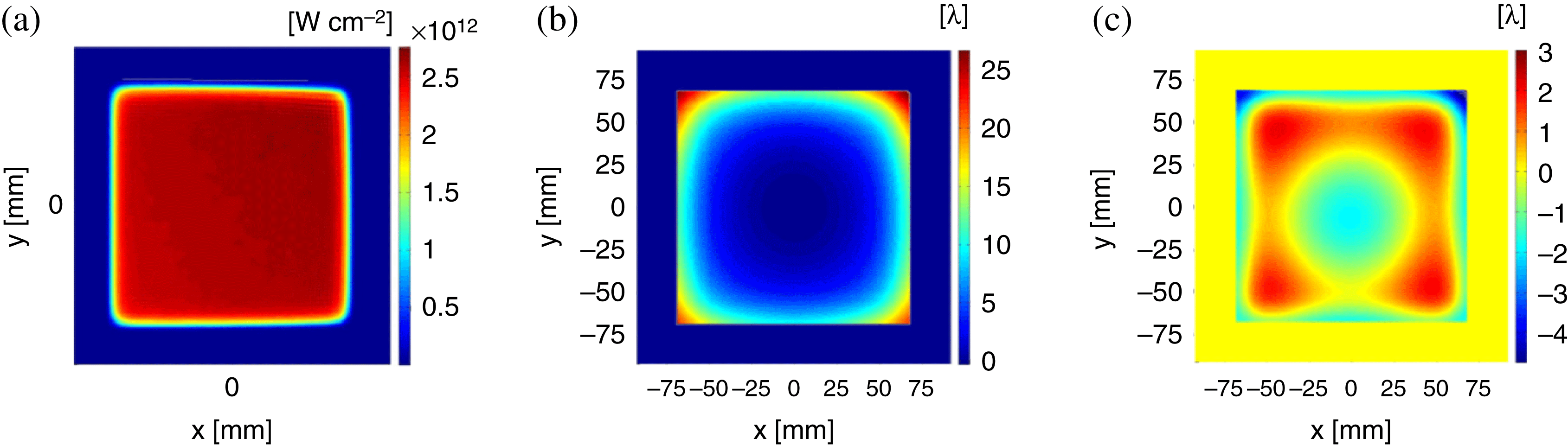
Figure 16. (a) Beam profile, (b) and (c) phase after subtraction of defocus and tilt of the output beam.

Figure 17. (a) The stress- and temperature-induced OPD after a single pass through the laser head (after one pass through eight slabs). (b) The depolarization of the beam after a single pass through the head caused by stress-induced birefringence. The  ${\mathrm{Cr}}^{4+}$:YAG cladding thickness was 20 mm.
The diffraction pattern in the beam is caused by shift of the beam due to large aberrations in the system and clipping of the beam. This can be remedied by decreasing the beam size considerably or by adding wavefront correction after each pass by implementing a DM in the laser chain (like NIF and LMJ). An optimized MIRO model which also includes the manufacturing defects of the optical components will be required in the future to provide a detailed understanding of the operational parameters of an optimized HiLASE laser design.
5. Thermal modeling
Substantial analysis has been performed in order to optimize the Yb:YAG gain medium size, coolant flow rates, arrangement of pumped and unpumped regions, and absorbing materials for properly designed (doping/width) cladding. The laser slabs are cooled by forced flow of He gas with a temperature of 190 K and a pressure of 5 bar. The model assumes that the energy deposition is the same for all slabs, which is a fair approximation given the stepped doping profile. A 3D finite-element method (FEM) using Comsol Multiphysics software was chosen to model the thermal effects in the amplifiers and the fluid dynamics of the helium flow. The calculation takes into account the temperature changes of the material parameters[Reference Aggarwal, Ripin, Ochoa and Fan14–Reference Ueda, Bisson, Yagi, Takaichi, Shirakawa, Yanagitani and Kaminskii16], the turbulent flow of the He and the resulting spatial variation of the heat transfer coefficient. The model is then used to calculate all mechanical stresses in the laser slab and birefringence depolarization losses for eight slabs according to the approach described in [Reference Bullington, Sutton, Bayramian, Caird, Deri, Erlandson and Henesian17]. The stress- and temperature-induced OPD and depolarization after one pass through eight slabs (i.e. one laser head) are shown in Figure 17. This figure shows a maximum OPD value of 8.9 waves and an average depolarization of 36.6%.
It is found that the thermal OPD and average depolarization can be substantially reduced by increasing the size of the cladding, and even more drastically by inserting a thin layer of undoped YAG around the gain medium[Reference Slezak, Lucianetti, Divoky, Sawicka and Mocek7] with the two-stepped doping profile of the  ${\mathrm{Cr}}^{4+}$:YAG cladding. The geometry and zone layout used for heat deposition modeling in the HiLASE amplifier (single and double clad configurations) are shown in Figure 18.

Figure 18. The geometry and zone layout used for heat deposition modeling in the HiLASE amplifier slab.

Figure 19. (a) The calculated OPD and (b) the depolarization loss due to eight slabs. A 3 mm layer of undoped YAG and two 25 mm Cr:YAG layers of cladding with different doping levels were added around the gain medium.
Table 1 summarizes the results of the three different layouts under consideration, i.e., single, enlarged single and double clad geometries. The enlarged single geometry had a cladding width of 53 mm, i.e., the same total cladding width as the double clad geometry consisting of a 3 mm layer of undoped YAG and two 25 mm layers of cladding with different doping levels.
Table 1. The Gain Medium and Cladding Dimensions used for Simulation of HiLASE Square Amplifiers.
Table 2. Thermal Results for HiLASE Square Amplifiers (Single, Enlarged Single, and Double Clad).
Figure 19 shows the total OPD and depolarization due to eight slabs in the double clad geometry.
Table 2 summarizes the thermal results for the single, enlarged single and double clad geometries. These results include the maximal temperature reached within the slab volume,  $T_{\mathrm{max}}$, the average temperature, $\langle T\rangle $, the total depolarization loss, $\gamma $, due to eight slabs (one amplifier head), the peak-to-valley (P-V) value of the OPD due to eight slabs, and the total eight-slab OPD with tilt and defocus subtracted.
The double clad geometry showed the minimum depolarization losses and OPD values. It should be noted that the tilted OPD profile in the double clad geometry is due to the helium gas flow which generates a transverse dependence of the heat transfer coefficient. However, the magnitude of the aberrations is well within the correction capability of the current DMs used for adaptive optics (AO)[Reference Pilar, Divoky, Sikocinski, Kmetik, Slezak, Lucianetti, Bonora and Mocek18]. These results suggest that a cryogenic helium gas approach coupled with properly designed (doping/width) cladding materials should be able to provide sufficient cooling capacity while introducing minimal optical distortions and thermal depolarization for operation of a kJ-class amplifier.
6. Wavefront correction
The calculated wavefront of the beam at the output of the laser system (see Figure 16) was corrected by a numerical model of a DM. We consider the worst condition for the amplifier of placing the DM after the last pass. The reliability of the wavefront correction code was verified experimentally in a slab simulator[Reference Pilar, Divoky, Sikocinski, Kmetik, Slezak, Lucianetti, Bonora and Mocek18]. The simulation was performed for a variable number of actuators from  $5\times 5$ to $8\times 8$. The numerical model for wavefront correction calculates influence functions from a plate equation describing bending of the thin face sheet for each individual actuator of the DM. Figure 20 shows the actuator layout of the DM, where ‘c’ is the size of the active region (or beam size) which is also characterized by the size ‘a’ of the actuators. The results have been calculated for different values of the ${\rm b}/{\rm c}$ ratio and stroke of the DM.

Figure 20. The actuator layout of the DM.
The deformation of the mirror is computed as a superposition of influence functions and the algorithm minimizes the OPD rms value. Figure 21 shows the residual rms values of the OPD as a function of the stroke after correction by the DM with  $6\times 6$ and $8\times 8$ actuators.

Figure 21. Residual rms values of the OPD as a function of the stroke after correction by the DM.
It is noted that the residual rms value after correction is more influenced by the  ${\rm b}/{\rm c}$ ratio than by the actuator density. Therefore, optimization of the DM requires large-area actuators outside the active region, i.e. large ${\rm b}/{\rm c}$ values rather than high actuator density. It should be noted that the larger the stroke is, the smaller the dynamic range used by the AO system will be. The DM is able to achieve numerical correction of the initial aberrations, as shown in Figure 22 ( ${\rm b}/{\rm c} = 0.43$, ${\rm stroke} = 12\ \mu {\rm m}$). The OPD after subtraction of defocus and tilt and the OPD corrected by the DM are shown in Figure 22. The rms value of the OPD was reduced from 0.56 waves down to 0.070 waves.

Figure 22. (a) The output wavefront calculated in MIRO and shown in Figure 16(a) after subtraction of tilt and defocus. (b) The residual wavefront after correction by the DM with  $8\times 8$ actuators ( ${\rm b}/{\rm c} = 0.43$, ${\rm stroke} = 12\ \mu {\rm m}$).
The corresponding far-field images before and after wavefront correction are shown in Figures 23(b) and (c). Figure 23(a) shows the far field with an ideal flat wavefront. The Strehl ratios of the aberrated and corrected beams are 0.083 and 0.971, respectively.

Figure 23. (a) Far field with ideal flat wavefront. (b) Far-field image before correction by the DM. (c) Far-field image after correction with  $8\times 8$ actuators ( ${\rm b}/{\rm c} = 0.43$, ${\rm stroke} = 12\ \mu {\rm m}$).
7. Frequency conversion
Frequency conversion of the fundamental wavelength at 1030 nm to the second and third harmonic wavelengths of 515 and 343 nm allows for more efficient absorption of laser energy by the deuterium–tritium target. In this section, we present the modeling results for the second harmonic generation (SHG) and third harmonic generation (THG) conversion efficiency. It is proposed to use LBO crystal for frequency conversion due to its excellent nonlinear properties and recently demonstrated large crystal sizes[Reference Hu, Zhao, Yue and Hu19]. RTP is also an interesting material for frequency conversion[Reference Oseledchik, Pisarevzsy, Prosvirnin, Starshenko and Svitanko20]. To the best of our knowledge, however, no multi-J/few-Hz operation of large-size RTP crystals has been reported so far. In addition, green absorption in RTP is much stronger than in LBO. Although the size of the LBO crystals that has been used in our calculations exceeds the currently available size, we believe that the required apertures will become available in the near future. The numerical simulations were performed using home-written code based on a three-wave interaction model, in which the symmetrized split-step method was used for calculations. A grid of  $128\times 128\times 128$ points was used for the 3D simulations. The spatial profile was assumed to be square shaped with dimensions of $140\ {\rm mm}\times 140\ {\rm mm}$. The intensity profile in the simulations was assumed to be ideal, i.e., to be defined by a super-Gaussian function of the 20th order for the spatial profile and of the eighth order for the temporal profile. To accommodate such a laser beam comfortably, the aperture of the LBO crystal was set to $160\ {\rm mm} \times 160\ {\rm mm}$. Since the shape of the pulse ideally ensures uniform intensity distribution in time and space, very high conversion efficiencies are easily achievable if significant wavefront distortions are absent. Figure 24 shows that SHG can achieve up to 90% conversion efficiency and even higher. In this calculation, the LBO crystal was oriented for type-I SHG, $XY$-plane, $\varphi =13.78^{\circ }$. We have assumed a fundamental wavelength pulse energy of 1 kJ, which corresponds to $1.32\ {\rm GW}\ {\rm cm}^{-2}$ peak intensity.

Figure 24. The SHG efficiency for different LBO thickness values.
As can be seen from Figure 24, the optimal LBO crystal thickness is close to 13 mm, with a theoretical conversion efficiency of more than 95%. For the case of THG, we investigated the most common setup where the second harmonic is first generated in LBO crystal (type-I,  $\sim $5 mm) with $\sim $60% efficiency. Then the pulses of both the first harmonic (FH) and the second harmonic are mixed in a second LBO crystal (type-II, o $+$ e
$+$ e  $=$ o) for sum-frequency generation (SFG). The second LBO crystal was oriented for type-II nonlinear interaction, $YZ$ plane, $\theta = 50.1^{\circ }$. The total THG conversion efficiency is shown in Figure 25. Several curves, representing different SHG conversion efficiencies in the first stage of the setup, are presented. In the optimized case, the maximum third harmonic output is obtained at $\sim $63% SHG conversion.

Figure 25. The THG efficiency for different LBO thickness values.
Angular and temperature acceptance are important parameters in the case of high energy and high average power operation. In the case of LBO type-I SHG at 1030 nm, we have calculated the angular acceptance using the Sellmeier equations to be 3.42 mrad cm (which yields 2.63 mrad for 13 mm crystal). For the THG via SFG in the given conditions, the angular acceptance was calculated to be 3.09 mrad cm (2.38 mrad for 13 mm crystal). For the temperature acceptance calculation, we currently rely on values provided by SNLO software, recalculated for the full width at half maximum (FWHM) of the  ${\rm sinc}^{2}(\Delta kL/2)$ function: 6.36 K cm for SHG and 3.19 K cm for THG (for 13 mm crystal 4.89 and 2.45 K accordingly). The acceptance values calculated above are useful for the comparison of different nonlinear crystals. However, in order to evaluate the actual angular tolerance of the crystal for a given pulse, we have also performed a numerical full 3D simulation for a set of angles in the vicinity of optimal phase matching. The simulation shows that the crystal detuning tolerance in this case is 0.93 mrad. We define this number as the FWHM level for the conversion efficiency function. The same simulation was performed for the second LBO crystal of 11.5 mm length, in which the third harmonic was generated via SFG, and it was shown that the crystal detuning tolerance in this case was 1.57 mrad. These simulations show that the output efficiency is more sensitive to angular detuning in the case of high efficiency of the frequency conversion processes and fundamental pulse depletion, in comparison to angular acceptance values calculated from the Sellmeier equations. It is noted that when phase and amplitude distortions become significant, the efficiency of the nonlinear process is expected to decrease. A more extensive model of the frequency convertor which includes amplitude or phase noise will be developed.
Acknowledgements
This work benefitted from the support of the Czech Republic’s Ministry of Education, Youth and Sports to the HiLASE (CZ.1.05/2.1.00/01.0027), DPSSLasers (CZ.1.07/2.3.00/20.0143), and Postdok (CZ.1.07/2.3.00/30.0057) projects, co-financed by the European Regional Development Fund. This research was supported by grant RVO 68407700. The authors would like to thank Dr. Audrius Zaukevicius from Vilnius Unversity for kindly providing his code for nonlinear interaction simulations.


 Open access