


1 Introduction
1.1 The Fargues–Fontaine curve
Let E be a local field and let C be a perfectoid field of characteristic p. For each such pair
 $(E,C)$
, Fargues and Fontaine have defined an E-scheme that we will denote by
$(E,C)$
, Fargues and Fontaine have defined an E-scheme that we will denote by
 ${\mathit {FF}}_E(C)$
– it is denoted by
${\mathit {FF}}_E(C)$
– it is denoted by
 $X_{C,E}$
in [Reference Fargues and FontaineFF, Def. 6.5.1]. It is in no sense a ‘curve over E’ or even a variety: it is not of finite type over E or over any other field. A scheme that is not of finite type over some base cannot be smooth or proper in the usual sense ([Reference Dieudonne and GrothendieckEGA, Vol 4, §17; Vol 2, §5]) and yet
$X_{C,E}$
in [Reference Fargues and FontaineFF, Def. 6.5.1]. It is in no sense a ‘curve over E’ or even a variety: it is not of finite type over E or over any other field. A scheme that is not of finite type over some base cannot be smooth or proper in the usual sense ([Reference Dieudonne and GrothendieckEGA, Vol 4, §17; Vol 2, §5]) and yet
 ${\mathit {FF}}_E(C)$
resembles a closed Riemann surface in some peculiar ways:
${\mathit {FF}}_E(C)$
resembles a closed Riemann surface in some peculiar ways:
-
• It is noetherian of Krull dimension 1. Moreover, it is regular, so that the local ring at each closed point of
 ${\mathit {FF}}_E(C)$
has a discrete valuation.
${\mathit {FF}}_E(C)$
has a discrete valuation. -
• A nonzero rational function f (that is, a section of
$\mathcal {O}_{{\mathit {FF}}}$
over the generic point) has
$v(f) \neq 0$
for at most finitely many of these valuations v and
$\sum _v v(f) = 0$
.


In fact,
 ${\mathit {FF}}_E(C)$
even resembles the Riemann sphere: one has
${\mathit {FF}}_E(C)$
even resembles the Riemann sphere: one has
 $H^1(\mathcal {O}_{FF}) = 0$
, and if C is algebraically closed, then
$H^1(\mathcal {O}_{FF}) = 0$
, and if C is algebraically closed, then
 $\operatorname {Pic}({\mathit {FF}}_E(C)) = \mathbf {Z}$
.
$\operatorname {Pic}({\mathit {FF}}_E(C)) = \mathbf {Z}$
.
There are some contrasts with the Riemann sphere:
 ${\mathit {FF}}_E(C)$
has indecomposable vector bundles of higher rank and for algebraically closed C its étale fundamental group is naturally isomorphic to the absolute Galois group of E. Fargues has a program to apply these properties of
${\mathit {FF}}_E(C)$
has indecomposable vector bundles of higher rank and for algebraically closed C its étale fundamental group is naturally isomorphic to the absolute Galois group of E. Fargues has a program to apply these properties of
 ${\mathit {FF}}_E(C)$
to the local Langlands correspondence [Reference FarguesFa].
${\mathit {FF}}_E(C)$
to the local Langlands correspondence [Reference FarguesFa].
When
 $E = \mathbf {Q}_p$
,
$E = \mathbf {Q}_p$
,
 ${\mathit {FF}}_E(C)$
is an important object in p-adic cohomology – it was introduced to organise some of the structures of p-adic Hodge theory. When
${\mathit {FF}}_E(C)$
is an important object in p-adic cohomology – it was introduced to organise some of the structures of p-adic Hodge theory. When
 $E = \mathbf {F}_p(\!(z)\!)$
, the analogous structures are those of Hartl [Reference HartlH]. We have nothing to say about
$E = \mathbf {F}_p(\!(z)\!)$
, the analogous structures are those of Hartl [Reference HartlH]. We have nothing to say about
 ${\mathit {FF}}_{\mathbf {Q}_p}(C)$
, but we are able to touch
${\mathit {FF}}_{\mathbf {Q}_p}(C)$
, but we are able to touch
 ${\mathit {FF}}_{\mathbf {F}_p(\!(z)\!)}(C)$
with mirror symmetry.
${\mathit {FF}}_{\mathbf {F}_p(\!(z)\!)}(C)$
with mirror symmetry.
1.2 Homological mirror symmetry
Homological mirror symmetry (HMS) is a framework for relating Lagrangian Floer theory on a symplectic manifold to the homological algebra of coherent sheaves on a scheme – often, a scheme that is seemingly unrelated to the symplectic manifold.
What symplectic structure could be mirror to
 ${\mathit {FF}}_{\mathbf {F}_p(\!(z)\!)}(C)$
? We suggest the answer is a 2-dimensional torus. There is already a very well-studied mirror relationship between the symplectic torus and the Tate elliptic curve (over
${\mathit {FF}}_{\mathbf {F}_p(\!(z)\!)}(C)$
? We suggest the answer is a 2-dimensional torus. There is already a very well-studied mirror relationship between the symplectic torus and the Tate elliptic curve (over
 $\mathbf {Z}(\!(t)\!)$
), which we review in Section 2. To get the Fargues–Fontaine curve in place of the Tate curve, we introduce two changes:
$\mathbf {Z}(\!(t)\!)$
), which we review in Section 2. To get the Fargues–Fontaine curve in place of the Tate curve, we introduce two changes:
-
1. We couple Lagrangian Floer theory to a locally constant sheaf of rings on the torus – the fibre of this sheaf of rings has characteristic p and going around one of the circles is the pth power map. (Going around the other circle is the identity map.)
-
2. We set the Novikov parameter (this is the element
$t \in \mathbf {Z}(\!(t)\!)$
in the ground ring of the Tate curve) to
$t = 1$
– symplectically, this is sort of like studying the limit as the symplectic form goes to
$0$
.


Both of these manoeuvres are unusual in symplectic geometry. The first turns out to be straightforward, so that one obtains a Fukaya
 $A_{\infty }$
-category with the usual properties. The second is much more delicate and touches some folklore questions about ‘convergent power series Floer homology’.
$A_{\infty }$
-category with the usual properties. The second is much more delicate and touches some folklore questions about ‘convergent power series Floer homology’.
1.3 Lagrangian Floer theory on the torus
Let T be a
 $2$
-dimensional torus, which we present as a quotient of
$2$
-dimensional torus, which we present as a quotient of
 $\mathbf {R}^2$
by
$\mathbf {R}^2$
by
 $\mathbf {Z}^2$
and endow with the standard symplectic form
$\mathbf {Z}^2$
and endow with the standard symplectic form
 $dx\,dy$
. For each integer m, let
$dx\,dy$
. For each integer m, let
 $L_{(m)} \subset T$
denote the image of the line in
$L_{(m)} \subset T$
denote the image of the line in
 $\mathbf {R}^2$
through the origin of slope
$\mathbf {R}^2$
through the origin of slope
 $-m$
. Let
$-m$
. Let
 $L_{(\infty )}$
denote the image of the vertical line through the origin. We orient
$L_{(\infty )}$
denote the image of the vertical line through the origin. We orient
 $L_{(m)}$
from left to right and
$L_{(m)}$
from left to right and
 $L_{(\infty )}$
from top to bottom. The figure shows
$L_{(\infty )}$
from top to bottom. The figure shows
 $L_{(0)}$
,
$L_{(0)}$
,
 $L_{(\infty )}$
and
$L_{(\infty )}$
and
 $L_{(3)}$
in a fundamental domain of T:
$L_{(3)}$
in a fundamental domain of T:

If
 $m_1> m_0$
, then
$m_1> m_0$
, then
 $L_{(m_1)}$
and
$L_{(m_1)}$
and
 $L_{(m_0)}$
meet transversely in
$L_{(m_0)}$
meet transversely in
 $(m_1 - m_0)$
points. Lagrangian Floer theory gives algebraic structures to the free modules
$(m_1 - m_0)$
points. Lagrangian Floer theory gives algebraic structures to the free modules
 $$ \begin{align} \mathrm{CF}(L_{(m_0)}, L_{(m_1)}) := \bigoplus_{x \in L_{(m_0)} \cap L_{(m_1)}} \Lambda, \end{align} $$
where
 $\Lambda $
is a suitable ring, about which more in Subsection 1.6. ‘
$\Lambda $
is a suitable ring, about which more in Subsection 1.6. ‘
 $\mathrm {CF}$
’ stands for ‘Floer cochains’. The orientations of
$\mathrm {CF}$
’ stands for ‘Floer cochains’. The orientations of
 $L_{(m_0)}, L_{(m_1)}$
endow (1.3.1) with a
$L_{(m_0)}, L_{(m_1)}$
endow (1.3.1) with a
 $\mathbf {Z}/2$
-grading (which can be lifted to a
$\mathbf {Z}/2$
-grading (which can be lifted to a
 $\mathbf {Z}$
-grading by making some additional topological choices) and
$\mathbf {Z}$
-grading by making some additional topological choices) and
 $\mathrm {CF}^*(L_{(m_0)},L_{(m_1)})$
supports a differential of degree
$\mathrm {CF}^*(L_{(m_0)},L_{(m_1)})$
supports a differential of degree
 $+1$
(Subsection 2.5). In the case at hand, these gradings are concentrated in a single degree 0 and the differential is zero.
$+1$
(Subsection 2.5). In the case at hand, these gradings are concentrated in a single degree 0 and the differential is zero.
We will return to the differential in Subsection 1.15 (and a little in Subsection 1.5), but to start we will be very interested in the ‘triangle product’
 $$ \begin{align} \mathrm{CF}(L_{(m_1)},L_{(m_2)}) \times \mathrm{CF}(L_{(m_0)},L_{(m_1)}) \to \mathrm{CF}(L_{(m_0)},L_{(m_2)}) \end{align} $$
whose value on
 $(x_1,x_2) \in (L_{(m_1)} \cap L_{(m_2)}) \times (L_{(m_0)} \cap L_{(m_1)})$
is the summation
$(x_1,x_2) \in (L_{(m_1)} \cap L_{(m_2)}) \times (L_{(m_0)} \cap L_{(m_1)})$
is the summation
 $$ \begin{align} \sum_{y \in L_{(m_0)} \cap L_{(m_2)}} y \left(\sum_{u \in \mathcal{M}(y,x_2,x_1)} \pm t^{\mathrm{area}(u)} \right). \end{align} $$
The inner sum is infinite: it is indexed by the set of rigid pseudoholomorphic triangles
 $$ \begin{align} u:\Delta^2 \to T \end{align} $$
with vertices at
 $x_1,x_2,y$
and one edge each along
$x_1,x_2,y$
and one edge each along
 $L_{(m_2)},L_{(m_1)},L_{(m_0)}$
. The sign in
$L_{(m_2)},L_{(m_1)},L_{(m_0)}$
. The sign in
 $\pm t^{\mathrm {area}(u)}$
depends on u and on the choice of a spin structure on each of the oriented
$\pm t^{\mathrm {area}(u)}$
depends on u and on the choice of a spin structure on each of the oriented
 $1$
-manifolds
$1$
-manifolds
 $L_{(m_i)}$
; see Subsection 2.4. In the present case it is possible to make those choices so that the signs are identically
$L_{(m_i)}$
; see Subsection 2.4. In the present case it is possible to make those choices so that the signs are identically
 $+1$
.
$+1$
.
1.4 Dehn twist
There is a canonical identification of
 $\mathrm {CF}(L_{(m)},L_{(n)})$
with
$\mathrm {CF}(L_{(m)},L_{(n)})$
with
 $\mathrm {CF}(L_{(0)},L_{(n-m)})$
, induced by
$\mathrm {CF}(L_{(0)},L_{(n-m)})$
, induced by
 $$ \begin{align*} (x,y) \mapsto (x,y-mx) \end{align*} $$
the m-fold Dehn twist around
 $L_{(\infty )}$
. An old suggestion of Seidel’s [Reference ZaslowZ] is to use this identification to package the triangle products as a graded ring structure on the sum
$L_{(\infty )}$
. An old suggestion of Seidel’s [Reference ZaslowZ] is to use this identification to package the triangle products as a graded ring structure on the sum
 $$ \begin{align} \Lambda \oplus \bigoplus_{m = 1}^{\infty} \mathrm{CF}(L_{(0)},L_{(m)}). \end{align} $$
The multiplication on (1.4.1) is associative and commutative for nontrivial reasons. The associativity is a consequence of a very general Floer-theoretic argument that studies
 $1$
-dimensional moduli spaces of pseudoholomorphic quadrilaterals (Subsection 2.11), and the commutativity is a consequence of a more particular observation about the Dehn twist [Reference ZaslowZ, §3].
$1$
-dimensional moduli spaces of pseudoholomorphic quadrilaterals (Subsection 2.11), and the commutativity is a consequence of a more particular observation about the Dehn twist [Reference ZaslowZ, §3].
1.5 The Floer cohomology of
$(L_{(0)},L_{(0)})$
In (1.4.1), we have inserted the unit of the ring by hand (the summand
 $\Lambda $
, which we place in degree 0), but this can also be motivated Floer-theoretically. The definition of
$\Lambda $
, which we place in degree 0), but this can also be motivated Floer-theoretically. The definition of
 $\mathrm {CF}$
in (1.3.1) is not the right one when
$\mathrm {CF}$
in (1.3.1) is not the right one when
 $L_{(m_0)} = L_{(m_1)}$
or for any other pair that do not meet transversely. But if
$L_{(m_0)} = L_{(m_1)}$
or for any other pair that do not meet transversely. But if
 $\phi = \{\phi ^s\}_{s \in \mathbf {R}}$
is a general Hamiltonian isotopy, then
$\phi = \{\phi ^s\}_{s \in \mathbf {R}}$
is a general Hamiltonian isotopy, then
 $$ \begin{align*} \mathrm{CF}(\phi^s L_{(0)},L_{(0)}) := \bigoplus_{x \in \phi^s L_{(0)} \cap L_{(0)}} x \cdot \Lambda, \end{align*} $$
together with its differential, gives a cochain complex whose cohomology groups do not depend on
 $\phi $
. These cohomology groups are
$\phi $
. These cohomology groups are
 $\mathbf {Z}/2$
-graded, and the
$\mathbf {Z}/2$
-graded, and the
 $\Lambda $
piece of (1.4.1) is naturally identified with
$\Lambda $
piece of (1.4.1) is naturally identified with
 $\mathrm {HF}^0(L_{(0)},L_{(0)})$
; cf. Subsection 2.12.
$\mathrm {HF}^0(L_{(0)},L_{(0)})$
; cf. Subsection 2.12.
1.6 Novikov ring
$\Lambda $
and Floer theory relative to a divisor

There is some flexibility in choosing the ground ring
 $\Lambda $
, but it should contain a ring of constants (let us use C for this ring – later on it will be the same as the C of Subsection 1.1) a parameter t and all necessary powers of it and it should carry a topology in which all the sums (1.4.1) converge. The conventional choice is the Novikov ring, which we will denote by
$\Lambda $
, but it should contain a ring of constants (let us use C for this ring – later on it will be the same as the C of Subsection 1.1) a parameter t and all necessary powers of it and it should carry a topology in which all the sums (1.4.1) converge. The conventional choice is the Novikov ring, which we will denote by
 $\Lambda _C$
:
$\Lambda _C$
:
 $$ \begin{align} \Lambda_C =\left\{\sum_{i = 0}^{\infty} a_i t^{\lambda_i} \mid a_i \in C, \lambda_i \in \mathbf{R} \text{ and } \lim_{i \to \infty} \lambda_i = \infty\right\}. \end{align} $$
We can shrink those coefficients to
 $C[\![t]\!]$
by the following device of Seidel’s, called Floer theory ‘relative to a divisor’. Rather than computing the area of the triangles u, we fix a basepoint
$C[\![t]\!]$
by the following device of Seidel’s, called Floer theory ‘relative to a divisor’. Rather than computing the area of the triangles u, we fix a basepoint
 $D \in T^2$
(in general, a symplectic divisor
$D \in T^2$
(in general, a symplectic divisor
 $D \subset T^2$
) and use the cardinality of
$D \subset T^2$
) and use the cardinality of
 $u^{-1}(D)$
in place of symplectic area. If D is in the first quadrant and extremely close to
$u^{-1}(D)$
in place of symplectic area. If D is in the first quadrant and extremely close to
 $(0,0)$
, then this cardinality is given by a simple formula which is independent of D unless the triangle u is extremely acute – let us write
$(0,0)$
, then this cardinality is given by a simple formula which is independent of D unless the triangle u is extremely acute – let us write
 $\mathrm {area}_{\mathbf {Z}}(u)$
for this discretised notion of area. With some additional care, by letting
$\mathrm {area}_{\mathbf {Z}}(u)$
for this discretised notion of area. With some additional care, by letting
 $D \to (0,0)$
(see [Reference Lekili and PerutzLPe2, §7.2.3] and [Reference Lekili and PerutzLPe2, Prop. 9.1]), we get a graded ring
$D \to (0,0)$
(see [Reference Lekili and PerutzLPe2, §7.2.3] and [Reference Lekili and PerutzLPe2, Prop. 9.1]), we get a graded ring
 $$ \begin{align} C[\![t]\!] \cdot 1 \oplus \bigoplus_{m = 1}^{\infty} \mathrm{CF}(L_{(0)},L_{(m)}). \end{align} $$
1.7 Theorem [Reference Lekili and PerutzLPe2]
The
 $C[\![t]\!]$
-scheme
$C[\![t]\!]$
-scheme
 $$ \begin{align} \operatorname{Proj}\left(C[\![t]\!] \cdot 1 \oplus \bigoplus_{m = 1}^{\infty} \mathrm{CF}(L_{(0)}, L_{(m)})\right) \end{align} $$
is isomorphic to
 $E_{\mathrm {Tate}} \times _{\mathbf {Z}[\![t]\!]} C[\![t]\!]$
; the Tate elliptic curve over
$E_{\mathrm {Tate}} \times _{\mathbf {Z}[\![t]\!]} C[\![t]\!]$
; the Tate elliptic curve over
 $C[\![t]\!]$
whose Weierstrass equation is
$C[\![t]\!]$
whose Weierstrass equation is
 $$ \begin{align*} y^2 + xy = x^3 - b_2 x - b_3 \end{align*} $$
where
 $b_2,b_3 \in \mathbf {Z}[\![t]\!]$
are the series
$b_2,b_3 \in \mathbf {Z}[\![t]\!]$
are the series
 $$ \begin{align} b_2 = \sum_{n = 1}^{\infty} 5n^3 \frac{t^n}{1-t^n} \qquad b_3 = \sum_{n =1}^{\infty} \left(\frac{7n^5 + 5n^3}{12}\right) \frac{t^n}{1-t^n}. \end{align} $$
1.8 Theta series
The relationship between (1.6.2) and functions on the Tate elliptic curve is more transparent when those functions are described in terms of
 $\theta $
-series. Set
$\theta $
-series. Set
 $$ \begin{align} \theta_{m,k} := \sum_{i = -\infty}^{\infty} t^{m \frac{i (i-1)}{2}+ k i}\, z^{mi + k}; \qquad \theta_{m,k}^{\mathrm{abs}} := \sum_{i = -\infty}^{\infty} t^{(mi+k)^2/(2m)} z^{mi+k}. \end{align} $$
The simplest of these series is the Jacobi function
 $$ \begin{align*} \theta_{1,0} = \sum_{i = -\infty}^{\infty} t^{\frac{i(i-1)}{2}} z^i = (1+z) \prod_{i = 1}^{\infty} \left[(1-t^i)(1+t^i z)(1+t^i z^{-1})\right]. \end{align*} $$
The other
 $\theta _{m,k}$
are obtained by a change of variables from
$\theta _{m,k}$
are obtained by a change of variables from
 $\theta _{1,0}$
. These series are doubly infinite in z, but in formally expanding the product of two of them, the coefficient of
$\theta _{1,0}$
. These series are doubly infinite in z, but in formally expanding the product of two of them, the coefficient of
 $z^i t^j$
has only finitely many nonzero contributions. The
$z^i t^j$
has only finitely many nonzero contributions. The
 $C[\![t]\!]$
-linear span of the
$C[\![t]\!]$
-linear span of the
 $\theta _{m,k}$
(respectively the
$\theta _{m,k}$
(respectively the
 $\Lambda _C$
-linear span the
$\Lambda _C$
-linear span the
 $\theta ^{\mathrm {abs}}_{m,k}$
) is closed under multiplication and graded by m and is isomorphic as a graded ring to (1.6.2) (or (1.4.1) in the absolute case). The isomorphisms send
$\theta ^{\mathrm {abs}}_{m,k}$
) is closed under multiplication and graded by m and is isomorphic as a graded ring to (1.6.2) (or (1.4.1) in the absolute case). The isomorphisms send
 $(k/m,0) \in L_{(0)} \cap L_{(m)}$
to
$(k/m,0) \in L_{(0)} \cap L_{(m)}$
to
 $\theta _{m,k}$
or to
$\theta _{m,k}$
or to
 $\theta ^{\mathrm {abs}}_{m,k}$
.
$\theta ^{\mathrm {abs}}_{m,k}$
.
1.9 Fukaya category and homological mirror symmetry
The triangle product (1.3.2) resembles a composition law in a category. It is part of a sequence of structures on the
 $\mathrm {CF}(L,L')$
,
$\mathrm {CF}(L,L')$
,
 $$ \begin{align} \mu_n:\mathrm{CF}(L_{n-1},L_n) \times \cdots \times \mathrm{CF}(L_0,L_1) \to \mathrm{CF}(L_0,L_n), \end{align} $$
that are obtained by summing over the
 $(n+1)$
-gons with sides along
$(n+1)$
-gons with sides along
 $L_0,L_1,\ldots ,L_n$
(Subsection 2.7). When one takes extra care to treat sets of Lagrangians that are not transverse (Subsection 2.12), these structures define an
$L_0,L_1,\ldots ,L_n$
(Subsection 2.7). When one takes extra care to treat sets of Lagrangians that are not transverse (Subsection 2.12), these structures define an
 $A_{\infty }$
-category. After passing to a triangulated envelope and splitting idempotents, we will call any of these
$A_{\infty }$
-category. After passing to a triangulated envelope and splitting idempotents, we will call any of these
 $A_{\infty }$
-structures a ‘Fukaya category’ and denote it by
$A_{\infty }$
-structures a ‘Fukaya category’ and denote it by
 $\mathrm {Fuk}(T)$
(in the absolute case) or
$\mathrm {Fuk}(T)$
(in the absolute case) or
 $\mathrm {Fuk}(T,D)$
(in the relative case).
$\mathrm {Fuk}(T,D)$
(in the relative case).
Kontsevich’s homological mirror symmetry conjecture, specialised to T, asks for a quasi-equivalence between
 $\mathrm {Fuk}(T)$
and the derived category of coherent sheaves on an elliptic curve. A version of this for complex elliptic curves was obtained in [Reference Polishchuk and ZaslowPoZa]. When
$\mathrm {Fuk}(T)$
and the derived category of coherent sheaves on an elliptic curve. A version of this for complex elliptic curves was obtained in [Reference Polishchuk and ZaslowPoZa]. When
 $C = \mathbf {Z}$
, Theorem 1.7, together with a generation result for
$C = \mathbf {Z}$
, Theorem 1.7, together with a generation result for
 $\mathrm {Fuk}(T,D)$
[Reference Lekili and PerutzLPe2, §6.3], constitute ‘homological mirror symmetry over
$\mathrm {Fuk}(T,D)$
[Reference Lekili and PerutzLPe2, §6.3], constitute ‘homological mirror symmetry over
 $\mathbf {Z}$
’:
$\mathbf {Z}$
’:
 $$ \begin{align*} \mathrm{Fuk}(T,D) \cong D^b(\operatorname{Coh}(E_{\mathrm{Tate}})). \end{align*} $$
The structure sheaf of
 $E_{\mathrm {Tate}}$
is the image of
$E_{\mathrm {Tate}}$
is the image of
 $L_{(0)}$
under this equivalence.
$L_{(0)}$
under this equivalence.
1.10 F-fields
Let
 $\underline {\Lambda }$
be a local system of rings on T, so that at each point
$\underline {\Lambda }$
be a local system of rings on T, so that at each point
 $x \in T$
we are given a ring
$x \in T$
we are given a ring
 $\underline {\Lambda }_x$
and along each path
$\underline {\Lambda }_x$
and along each path
 $\gamma $
from x to y we are given a ring isomorphism
$\gamma $
from x to y we are given a ring isomorphism
 $$ \begin{align} \nabla \gamma:\underline{\Lambda}_x \stackrel{\sim}{\to} \underline{\Lambda}_y. \end{align} $$
Suppose that each ring
 $\underline {\Lambda }_x$
has the structures that we asked for in Subsection 1.6: it contains a ring of constants (we can denote it by
$\underline {\Lambda }_x$
has the structures that we asked for in Subsection 1.6: it contains a ring of constants (we can denote it by
 $\underline {C}_x$
) and distinguished elements of the form
$\underline {C}_x$
) and distinguished elements of the form
 $t^a$
and carries a topology. The maps (1.10.1) should be continuous and carry each
$t^a$
and carries a topology. The maps (1.10.1) should be continuous and carry each
 $\underline {C}_x$
to
$\underline {C}_x$
to
 $\underline {C}_y$
but leave the elements of the form
$\underline {C}_y$
but leave the elements of the form
 $t^a$
alone (
$t^a$
alone (
 $\nabla \gamma (t^a) = t^a)$
.
$\nabla \gamma (t^a) = t^a)$
.
We will develop a version of Floer theory ‘with coefficients in
 $\underline {\Lambda }$
’. As in Subsection 1.6, we could work either relative to a divisor or absolutely. In the relative case, we would take
$\underline {\Lambda }$
’. As in Subsection 1.6, we could work either relative to a divisor or absolutely. In the relative case, we would take
 $\underline {\Lambda } := \underline {C}[\![t]\!]$
, where
$\underline {\Lambda } := \underline {C}[\![t]\!]$
, where
 $\underline {C}$
is a locally constant sheaf of rings. In the absolute case, we would take
$\underline {C}$
is a locally constant sheaf of rings. In the absolute case, we would take
 $\underline {\Lambda } := \Lambda _{\underline {C}}$
(1.6.1).
$\underline {\Lambda } := \Lambda _{\underline {C}}$
(1.6.1).
In the example of interest to us, the sheaf of rings is pulled back from
 $S^1$
, along the projection map
$S^1$
, along the projection map
 $$ \begin{align} \mathfrak{f}:T \to S^1. \end{align} $$
Then
 $\underline {\Lambda }$
is determined by a ring C and an automorphism (the monodromy around the base
$\underline {\Lambda }$
is determined by a ring C and an automorphism (the monodromy around the base
 $S^1$
)
$S^1$
)
 $\sigma $
of C. It induces an automorphism of
$\sigma $
of C. It induces an automorphism of
 $C[\![t]\!]$
and of
$C[\![t]\!]$
and of
 $\Lambda _C$
that fixes each
$\Lambda _C$
that fixes each
 $t^a$
. We are interested in the case when C is perfect of characteristic p and
$t^a$
. We are interested in the case when C is perfect of characteristic p and
 $\sigma $
is the pth root map.
$\sigma $
is the pth root map.
The map (1.10.2) (and the monodromy map
 $\sigma $
) is just for book-keeping, but it also has an ‘occult’ interpretation, in a way fitting in to the old analogy between number fields and 3-manifolds and between primes and knots. The generator in the fundamental group of the base circle
$\sigma $
) is just for book-keeping, but it also has an ‘occult’ interpretation, in a way fitting in to the old analogy between number fields and 3-manifolds and between primes and knots. The generator in the fundamental group of the base circle
 $S^1$
and the Frobenius in the absolute Galois group of
$S^1$
and the Frobenius in the absolute Galois group of
 $\mathbf {F}_p$
act on C in the same way: by pth powers. See [Reference TreumannT] for a little bit more about this. There is also a natural map from the set of closed points of
$\mathbf {F}_p$
act on C in the same way: by pth powers. See [Reference TreumannT] for a little bit more about this. There is also a natural map from the set of closed points of
 ${\mathit {FF}}_E(C)$
(for
${\mathit {FF}}_E(C)$
(for
 $E = \mathbf {F}_p(\!(z)\!)$
or any other local field) to
$E = \mathbf {F}_p(\!(z)\!)$
or any other local field) to
 $S^1$
, and in some sense this article explores the idea that the SYZ mechanism for mirror symmetry could apply (Subsection 4.5).
$S^1$
, and in some sense this article explores the idea that the SYZ mechanism for mirror symmetry could apply (Subsection 4.5).
1.11 Lagrangian Floer theory – coupled to
$\underline {\Lambda }$

Let us put
 $$ \begin{align} \mathrm{CF}(L_{(m_0)},L_{(m_1)};\underline{\Lambda}) := \bigoplus_{x \in L_{(m_0)} \cap L_{(m_1)}} \underline{\Lambda}_x. \end{align} $$
Lagrangian Floer theory coupled to
 $\underline {\Lambda }$
concerns algebraic structures on (1.11.1); for instance, a triangle product
$\underline {\Lambda }$
concerns algebraic structures on (1.11.1); for instance, a triangle product
 $$ \begin{align} \mathrm{CF}(L_{(m_1)},L_{(m_2)};\underline{\Lambda}) \times \mathrm{CF}(L_{(m_0)},L_{(m_1)};\underline{\Lambda}) \to \mathrm{CF}(L_{(m_0)},L_{(m_2)};\underline{\Lambda}). \end{align} $$
In some sense, (1.11.1) is another free
 $\Lambda $
-module on the intersection points
$\Lambda $
-module on the intersection points
 $L_{(m_0)} \cap L_{(m_1)}$
but with many different
$L_{(m_0)} \cap L_{(m_1)}$
but with many different
 $\Lambda $
-module structures. The product (1.11.2) is not
$\Lambda $
-module structures. The product (1.11.2) is not
 $\Lambda $
-bilinear with respect to any of them. To define it, we give its value on a pair
$\Lambda $
-bilinear with respect to any of them. To define it, we give its value on a pair
 $$ \begin{align} (x_2 \cdot b,x_1 \cdot a) \in \mathrm{CF}(L_{(m_1)},L_{(m_2)};\underline{\Lambda}) \times \mathrm{CF}(L_{(m_0)},L_{(m_1)};\underline{\Lambda}) \end{align} $$
for any
 $a \in \underline {\Lambda }_{x_1}$
and
$a \in \underline {\Lambda }_{x_1}$
and
 $b \in \underline {\Lambda }_{x_2}$
and extend bi-additively (or, more precisely,
$b \in \underline {\Lambda }_{x_2}$
and extend bi-additively (or, more precisely,
 $\Lambda _{\mathbf {Z}}$
-bilinearly). The value on
$\Lambda _{\mathbf {Z}}$
-bilinearly). The value on
 $(x_2 \cdot b,x_1 \cdot a)$
is
$(x_2 \cdot b,x_1 \cdot a)$
is
 $$ \begin{align} \sum_{y \in L_{(m_0)} \cap L_{(m_2)}} y \sum_{u \in \mathcal{M}(y,x_2,x_1)} \pm t^{\mathrm{area}(u) \text{ or } \mathrm{area}_{\mathbf{Z}}(u)} \nabla \gamma_2(b \nabla \gamma_1(a \nabla \gamma_0(1))) \end{align} $$
where
 $\gamma _0:y \to x_1$
,
$\gamma _0:y \to x_1$
,
 $\gamma _1:x_1 \to x_2$
and
$\gamma _1:x_1 \to x_2$
and
 $\gamma _2:x_2 \to y$
are the three sides of the triangle u, appearing in counterclockwise order.
$\gamma _2:x_2 \to y$
are the three sides of the triangle u, appearing in counterclockwise order.

The
 $\pm $
signs in the formula (1.11.4) are the same as they are in (1.3.3); in particular, one can arrange that they are identically
$\pm $
signs in the formula (1.11.4) are the same as they are in (1.3.3); in particular, one can arrange that they are identically
 $+1$
.
$+1$
.
When the monodromy of
 $\underline {\Lambda }$
around
$\underline {\Lambda }$
around
 $L_{(\infty )}$
is trivial – equivalently, when
$L_{(\infty )}$
is trivial – equivalently, when
 $\underline {\Lambda }$
is pulled back along (1.10.2) – it is possible to package these triangle products into a graded ring structure:
$\underline {\Lambda }$
is pulled back along (1.10.2) – it is possible to package these triangle products into a graded ring structure:
 $$ \begin{align} \bigoplus_{m = 1}^{\infty} \mathrm{CF}(L_{(0)},L_{(m)};\underline{\Lambda}). \end{align} $$
1.12 Theorem
For each
 $a \in C$
and each pair of integers
$a \in C$
and each pair of integers
 $m,k$
with
$m,k$
with
 $m> k \geq 0$
, let
$m> k \geq 0$
, let
 $\theta _{m,k}[a]$
denote the formal series
$\theta _{m,k}[a]$
denote the formal series
 $$ \begin{align*} \theta_{m,k}[a] := \sum_{i = -\infty}^{\infty} t^{m\frac{i(i-1)}{2}+ki} z^{mi+k} \sigma^i(a) \end{align*} $$
Let
 $\theta ^{\mathrm {abs}}_{m,k}[a]$
denote the formal series
$\theta ^{\mathrm {abs}}_{m,k}[a]$
denote the formal series
 $$ \begin{align*} \theta^{\mathrm{abs}}_{m,k}[a] := \sum_{i = -\infty}^{\infty} t^{\frac{1}{2m} (m i +k)^2} z^{mi+k} \sigma^i(a). \end{align*} $$
Then the relative (respectively absolute) version of (1.11.5) is isomorphic, as a ring-without-unit, to the
 $\mathbf {Z}[\![t]\!]$
-linear span of the
$\mathbf {Z}[\![t]\!]$
-linear span of the
 $\theta _{m,k}[a]$
(respectively to the
$\theta _{m,k}[a]$
(respectively to the
 $\Lambda _{\mathbf {Z}}$
-linear span of the
$\Lambda _{\mathbf {Z}}$
-linear span of the
 $\theta ^{\mathrm {abs}}_{m,k}[a]$
).
$\theta ^{\mathrm {abs}}_{m,k}[a]$
).
1.13 Specialisations of t
Fix a commutative ring C and an automorphism
 $\sigma $
; cf. (1.10.2). The groups (1.11.1) are linear over
$\sigma $
; cf. (1.10.2). The groups (1.11.1) are linear over
 $\Lambda _C^{\sigma }$
in the absolute case and over
$\Lambda _C^{\sigma }$
in the absolute case and over
 $C^{\sigma }[\![t]\!]$
in the relative case. We will discuss the specialisations
$C^{\sigma }[\![t]\!]$
in the relative case. We will discuss the specialisations
 $t = 0$
and
$t = 0$
and
 $t = 1$
. The case
$t = 1$
. The case
 $t = 0$
we treat only briefly in Subsection 4.1 – the absolute case is not of interest, while the relative case is parallel to the ‘large volume limit’ of T and its mirror relationship with the nodal cubic curve at the ‘large complex structure limit’.
$t = 0$
we treat only briefly in Subsection 4.1 – the absolute case is not of interest, while the relative case is parallel to the ‘large volume limit’ of T and its mirror relationship with the nodal cubic curve at the ‘large complex structure limit’.
The case
 $t = 1$
is more delicate. There is a class of symplectic manifolds and Lagrangian submanifolds (for instance, monotone Lagrangians in a Fano manifold, or in a genus 2 surface) for which setting
$t = 1$
is more delicate. There is a class of symplectic manifolds and Lagrangian submanifolds (for instance, monotone Lagrangians in a Fano manifold, or in a genus 2 surface) for which setting
 $t = 1$
is unproblematic, but the torus does not belong to this class. And, indeed, the series (1.3.3), (1.7.2) do not converge, in any Archimedean or non-Archimedean ring, when
$t = 1$
is unproblematic, but the torus does not belong to this class. And, indeed, the series (1.3.3), (1.7.2) do not converge, in any Archimedean or non-Archimedean ring, when
 $t = 1$
.
$t = 1$
.
An F-field can repair some (but only some) of the convergence. Define
 $$ \begin{align} \mathrm{CF}(L_{(m_0)},L_{(m_1)};\underline{C}) = \bigoplus_{x \in L_{(m_0)} \cap L_{(m_1)}} \underline{C}_x. \end{align} $$
Setting
 $t = 1$
in (1.11.4) suggests, in a formal way, a map
$t = 1$
in (1.11.4) suggests, in a formal way, a map
 $$ \begin{align*} \mathrm{CF}(L_{(m_1)},L_{(m_2)};\underline{C}) \times \mathrm{CF}(L_{(m_0)},L_{(m_1)};\underline{C}) \dashrightarrow \mathrm{CF}(L_{(m_0)},L_{(m_2)};\underline{C}). \end{align*} $$
When C is complete with respect to a norm
 $|\cdot |$
,
$|\cdot |$
,
 $\sigma $
is the pth root map and
$\sigma $
is the pth root map and
 $m_0 < m_1 < m_2$
, this map has a nontrivial domain of convergence. In particular, it defines a multiplication on
$m_0 < m_1 < m_2$
, this map has a nontrivial domain of convergence. In particular, it defines a multiplication on
 $$ \begin{align} \bigoplus_{m> 0} \mathrm{CF}(L_{(0)},L_{(m)};\underline{\mathfrak{m}}) \end{align} $$
where
 $\mathfrak {m} = \{x \in C : |x| < 1\}$
.
$\mathfrak {m} = \{x \in C : |x| < 1\}$
.
1.14 The Fargues–Fontaine graded ring
A perfect field of characteristic p, complete with respect to a norm
 $|\cdot |$
, is since [Reference ScholzeSc] known as a ‘perfectoid field of characteristic p’. Suppose
$|\cdot |$
, is since [Reference ScholzeSc] known as a ‘perfectoid field of characteristic p’. Suppose
 $(C,|\cdot |)$
is such a field and suppose furthermore that C is algebraically closed. Let
$(C,|\cdot |)$
is such a field and suppose furthermore that C is algebraically closed. Let
 $E = \mathbf {F}_p(\!(z)\!)$
and let
$E = \mathbf {F}_p(\!(z)\!)$
and let
 $B \supset E$
be the set of bi-infinite formal series
$B \supset E$
be the set of bi-infinite formal series
 $\sum _{i \in \mathbf {Z}} b_i z^i \in \prod _{i \in \mathbf {Z}} C z^i$
with coefficients
$\sum _{i \in \mathbf {Z}} b_i z^i \in \prod _{i \in \mathbf {Z}} C z^i$
with coefficients
 $b_i \in C$
and which obey
$b_i \in C$
and which obey
 $$ \begin{align} \forall r \in (0,1) \qquad |b_i| r^i \to 0 \text{ as } |i| \to \infty. \end{align} $$
This ring B coincides with what is called
 $B_{(0,1)}$
in [Reference Fargues and FontaineFF, Ex. 1.6.5] and what is called
$B_{(0,1)}$
in [Reference Fargues and FontaineFF, Ex. 1.6.5] and what is called
 $\mathcal {O}_{\mathbf {R}^1}((0,1))$
in [Reference Kontsevich and SoibelmanKS, Def. 21].
$\mathcal {O}_{\mathbf {R}^1}((0,1))$
in [Reference Kontsevich and SoibelmanKS, Def. 21].
The automorphism
 $\varphi :B \to B$
given by
$\varphi :B \to B$
given by
 $$ \begin{align} \varphi:\left(\sum c_i z^i\right) \mapsto \sum c_i^p z^i \qquad (\text{i.e. } \varphi(f(z)) = f(z^{1/p})^p) \end{align} $$
cuts B into ‘eigenspaces’
 $ B^{\varphi = z^n} := \left \{f \in B \mid \varphi (f) = z^n f \right \} $
. The Fargues–Fontaine curve attached to
$ B^{\varphi = z^n} := \left \{f \in B \mid \varphi (f) = z^n f \right \} $
. The Fargues–Fontaine curve attached to
 $(E,C)$
is
$(E,C)$
is
 $$ \begin{align} {\mathit{FF}}_E(C):=\operatorname{Proj}\left(\bigoplus_{n = 0}^{\infty} B^{\varphi = z^n}\right). \end{align} $$

1.15 Annuli
The degree 0 piece
 $B^{\varphi = 1}$
of the Fargues–Fontaine graded ring (1.14.3) is isomorphic to E (
$B^{\varphi = 1}$
of the Fargues–Fontaine graded ring (1.14.3) is isomorphic to E (
 $= \mathbf {F}_p(\!(z)\!)$
in our case). The theorem (1.14.4) does not explain how this part arises Floer-theoretically. As in Subsection 1.5, it should come from the Floer cohomology of
$= \mathbf {F}_p(\!(z)\!)$
in our case). The theorem (1.14.4) does not explain how this part arises Floer-theoretically. As in Subsection 1.5, it should come from the Floer cohomology of
 $L_{(0)}$
against itself – a version of Floer cohomology with the F-field turned on – but the usual rules for making sense of the nontransverse intersection
$L_{(0)}$
against itself – a version of Floer cohomology with the F-field turned on – but the usual rules for making sense of the nontransverse intersection
 $L_{(0)} \cap L_{(0)}$
have to be revisited when
$L_{(0)} \cap L_{(0)}$
have to be revisited when
 $t = 1$
.
$t = 1$
.
As we mentioned in Subsection 1.5 and review in Subsection 2.13, the usual rules involve choosing a Hamiltonian isotopy
 $\{\phi ^s\}_{s \in \mathbf {R}}$
so that
$\{\phi ^s\}_{s \in \mathbf {R}}$
so that
 $\phi ^s L_{(0)}$
and
$\phi ^s L_{(0)}$
and
 $L_{(0)}$
do meet transversely. The problem that we encounter is that the quasi-isomorphism type of
$L_{(0)}$
do meet transversely. The problem that we encounter is that the quasi-isomorphism type of
 $\mathrm {CF}(\phi ^s L_{(0)},L_{(0)};\underline {C})$
, with its bigon differential, is no longer independent of
$\mathrm {CF}(\phi ^s L_{(0)},L_{(0)};\underline {C})$
, with its bigon differential, is no longer independent of
 $\phi $
. One still has natural maps between cochain complexes for different
$\phi $
. One still has natural maps between cochain complexes for different
 $\phi $
, but they are not quasi-isomorphisms: the usual formula for the necessary cochain homotopies does not converge.
$\phi $
, but they are not quasi-isomorphisms: the usual formula for the necessary cochain homotopies does not converge.
This is a well-known problem with ‘convergent power series Floer cohomology’. It is discussed in print in [Reference Cho and OhChOh, p.3] and [Reference AurouxAur2, §4.2] and perhaps elsewhere, but there is not much theory available for addressing it. Still, we take the following point of view (which is only heuristic):
‘Continuation’ – that is, the independence of the Hamiltonian displacement
 $\phi $
– fails because there are pseudoholomorphic annuli in T that have one side on
$\phi $
– fails because there are pseudoholomorphic annuli in T that have one side on
 $\phi ^s L_{(0)}$
and the other side on
$\phi ^s L_{(0)}$
and the other side on
 $L_{(0)}$
.
$L_{(0)}$
.
For instance, Ozsváth and Szabó stick to ‘admissible’ Heegaard diagrams to avoid problems with annuli like these [Reference Ozsváth and SzabóOzSz, §4.2.2]. The problem they pose in Lagrangian Floer theory is closely related to the problem that closed gradient orbits pose in circle-valued Morse theory [Reference Hutchings and LeeHuLe]. There is some speculation about incorporating them directly into Floer-theoretic invariants in [Reference AurouxAur2].
1.16 Loud Floer cochains
If L and
 $L'$
are in different homology classes, there are no annuli between them. But there are infinitely many annuli between
$L'$
are in different homology classes, there are no annuli between them. But there are infinitely many annuli between
 $\phi ^s L_{(0)}$
and
$\phi ^s L_{(0)}$
and
 $L_{(0)}$
for any
$L_{(0)}$
for any
 $\phi $
. If we fix an ‘autonomous’
$\phi $
. If we fix an ‘autonomous’
 $\phi $
, then we can get these under control by considering larger and larger s: for s large, all of the annuli between
$\phi $
, then we can get these under control by considering larger and larger s: for s large, all of the annuli between
 $\phi ^s L_{(0)}$
and
$\phi ^s L_{(0)}$
and
 $L_{(0)}$
have large area. For instance,
$L_{(0)}$
have large area. For instance,

Some of the constructions of [Reference LeeLee] have inspired us here. The complexes
 $\mathrm {CF}(\phi ^s L_{(0)},L_{(0)};\underline {C})$
for different s do not all have the same cohomology, but there are natural cochain maps
$\mathrm {CF}(\phi ^s L_{(0)},L_{(0)};\underline {C})$
for different s do not all have the same cohomology, but there are natural cochain maps
 $$ \begin{align*} \mathrm{CF}(\phi^s L_{(0)},L_{(0)};\underline{C}) \to \mathrm{CF}(\phi^{s'} L_{(0)},L_{(0)};\underline{C}) \end{align*} $$
whenever
 $s'> s$
. We will study the colimit of this filtered diagram. For large s, the picture of
$s'> s$
. We will study the colimit of this filtered diagram. For large s, the picture of
 $\phi ^s L_{(0)}$
is a sine wave with large amplitude (wrapped up around the torus). We call
$\phi ^s L_{(0)}$
is a sine wave with large amplitude (wrapped up around the torus). We call
 $$ \begin{align} \mathrm{CF}_{\mathrm{loud}}(L_{(0)},L_{(0)};\underline{C}) := \varinjlim_s \mathrm{CF}(\phi^s L_{(0)},L_{(0)};\underline{C}) \end{align} $$
the loud Floer cochains on
 $(L_{(0)},L_{(0)})$
. The name was suggested to us by Johnson-Freyd. Now our point of view is the following:
$(L_{(0)},L_{(0)})$
. The name was suggested to us by Johnson-Freyd. Now our point of view is the following:
By shouting infinitely loud, all of the annuli break, along with whatever problems they posed for noninvariance.
We will not try to make this precise, but for a somewhat analogous precedent in the setting of periodic orbits, see what is called the ‘Latour trick’ in [Reference HutchingsHutc]. The Latour trick breaks up the periodic orbits of a closed
 $1$
-form by adding a large multiple of an exact
$1$
-form by adding a large multiple of an exact
 $1$
-form. One could equivalently think of pushing the graph of the closed
$1$
-form. One could equivalently think of pushing the graph of the closed
 $1$
-form, for a long time, by the Hamiltonian flow of a primitive for the exact form. A large finite multiple of the exact form suffices to break up all the periodic orbits, while in (1.16.1) one has to pass to the limit, but maybe ‘shouting loud’ is not a worse metaphor for one process than for the other.
$1$
-form, for a long time, by the Hamiltonian flow of a primitive for the exact form. A large finite multiple of the exact form suffices to break up all the periodic orbits, while in (1.16.1) one has to pass to the limit, but maybe ‘shouting loud’ is not a worse metaphor for one process than for the other.
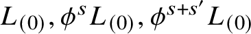
We will show that the triangles with sides on
 $L_{(0)}, \phi ^s L_{(0)}, \phi ^{s+s'} L_{(0)}$
induce a multiplication on
$L_{(0)}, \phi ^s L_{(0)}, \phi ^{s+s'} L_{(0)}$
induce a multiplication on
 $\mathrm {CF}_{\mathrm {loud}}(L_{(0)},L_{(0)};\underline {C})$
and on
$\mathrm {CF}_{\mathrm {loud}}(L_{(0)},L_{(0)};\underline {C})$
and on
 $\mathrm {HF}_{\mathrm {loud}}(L_{(0)},L_{(0)};\underline {C})$
. Our construction of this multiplication is quite crude: a better analysis would follow the construction of an
$\mathrm {HF}_{\mathrm {loud}}(L_{(0)},L_{(0)};\underline {C})$
. Our construction of this multiplication is quite crude: a better analysis would follow the construction of an
 $A_{\infty }$
-structure on wrapped Floer cochains [Reference Abouzaid and SeidelAS], which we expect to apply here and give a richer structure. But our computations give an isomorphism of rings
$A_{\infty }$
-structure on wrapped Floer cochains [Reference Abouzaid and SeidelAS], which we expect to apply here and give a richer structure. But our computations give an isomorphism of rings
 $$ \begin{align} \mathrm{HF}^0_{\mathrm{loud}}(L_{(0)},L_{(0)};\underline{C}) \cong C^{\sigma}[z,z^{-1}]. \end{align} $$
When
 $\sigma $
is the pth root map, this is the Laurent polynomial ring
$\sigma $
is the pth root map, this is the Laurent polynomial ring
 $\mathbf {F}_p[z,z^{-1}]$
, a dense subring of
$\mathbf {F}_p[z,z^{-1}]$
, a dense subring of
 $\mathbf {F}_p(\!(z)\!)$
.
$\mathbf {F}_p(\!(z)\!)$
.
One can similarly define
 $\mathrm {HF}_{\mathrm {loud}}(L_{(m)},L_{(m)};\underline {C})$
and a ring structure on it, for any
$\mathrm {HF}_{\mathrm {loud}}(L_{(m)},L_{(m)};\underline {C})$
and a ring structure on it, for any
 $m \in \mathbf {Q}$
. One gets the same answer (1.16.2) when m is an integer. For
$m \in \mathbf {Q}$
. One gets the same answer (1.16.2) when m is an integer. For
 $m = d/r$
, we expect but will not prove that
$m = d/r$
, we expect but will not prove that
 $\mathrm {HF}^0_{\mathrm {loud}}$
is a dense subring of an
$\mathrm {HF}^0_{\mathrm {loud}}$
is a dense subring of an
 $r^2$
-dimensional division algebra over
$r^2$
-dimensional division algebra over
 $\mathbf {F}_p(\!(z)\!)$
whose invariant is
$\mathbf {F}_p(\!(z)\!)$
whose invariant is
 $m+\mathbf {Z} \in \mathbf {Q}/\mathbf {Z}$
. The indecomposable vector bundles on the Fargues–Fontaine curve are classified by
$m+\mathbf {Z} \in \mathbf {Q}/\mathbf {Z}$
. The indecomposable vector bundles on the Fargues–Fontaine curve are classified by
 $\mathbf {Q}$
, and those division algebras arise as their endomorphism rings [Reference Fargues and FontaineFF, Thm. 8.2.10].
$\mathbf {Q}$
, and those division algebras arise as their endomorphism rings [Reference Fargues and FontaineFF, Thm. 8.2.10].
2 Some Floer-theoretic background
In this section we review some of Floer theory, making what simplifications are possible when the target manifold is a 2d torus T.
2.1 J-holomorphic polygons
Let
 $D \subset \mathbf {C}$
be the closed unit disk in the complex plane. We denote by
$D \subset \mathbf {C}$
be the closed unit disk in the complex plane. We denote by
 $D^{\circ }$
the open unit disk and
$D^{\circ }$
the open unit disk and
 $\partial D = D - D^{\circ }$
the boundary of D. Let
$\partial D = D - D^{\circ }$
the boundary of D. Let
 $\mathbf {z} = (z_0,\ldots ,z_n)$
denote an ordered
$\mathbf {z} = (z_0,\ldots ,z_n)$
denote an ordered
 $(n+1)$
-tuple of points in
$(n+1)$
-tuple of points in
 $\partial D$
. We require that the points of
$\partial D$
. We require that the points of
 $\mathbf {z}$
are pairwise distinct and that the counterclockwise arc subtending
$\mathbf {z}$
are pairwise distinct and that the counterclockwise arc subtending
 $z_{i-1}$
and
$z_{i-1}$
and
 $z_i$
(or
$z_i$
(or
 $z_n$
and
$z_n$
and
 $z_0$
) does not contain any other point of
$z_0$
) does not contain any other point of
 $\mathbf {z}$
.
$\mathbf {z}$
.
Let
 $L_0,L_1,\ldots ,L_n$
be an
$L_0,L_1,\ldots ,L_n$
be an
 $(n+1)$
-tuple of 1-dimensional submanifolds of T and let
$(n+1)$
-tuple of 1-dimensional submanifolds of T and let
 $(x_0,\ldots ,x_n)$
be a tuple of points in T with
$(x_0,\ldots ,x_n)$
be a tuple of points in T with
 $$ \begin{align*} x_0 \in L_0 \cap L_n, \qquad x_1 \in L_1 \cap L_0, \qquad \ldots,\qquad x_n \in L_n \cap L_{n-1}. \end{align*} $$
We write
 $\mathcal {W}(x_0,\ldots ,x_n)$
for the set of pairs
$\mathcal {W}(x_0,\ldots ,x_n)$
for the set of pairs
 $(\mathbf {z},u)$
where
$(\mathbf {z},u)$
where
 $u:D \to T$
is a continuous map, smooth away from
$u:D \to T$
is a continuous map, smooth away from
 $\mathbf {z}$
, that carries
$\mathbf {z}$
, that carries
 $z_i$
to
$z_i$
to
 $x_i$
and that maps the counterclockwise arc between
$x_i$
and that maps the counterclockwise arc between
 $z_i$
and
$z_i$
and
 $z_{i+1}$
into
$z_{i+1}$
into
 $L_i$
. It carries a topology in which a sequence
$L_i$
. It carries a topology in which a sequence
 $(\mathbf {z}_i,u_i)$
converges
$(\mathbf {z}_i,u_i)$
converges
 $(\mathbf {z},u)$
if
$(\mathbf {z},u)$
if
 $\mathbf {z}_i \to \mathbf {z}$
in
$\mathbf {z}_i \to \mathbf {z}$
in
 $(\partial D)^{\times (n+1)}$
and
$(\partial D)^{\times (n+1)}$
and
 $u_i \to u$
in a suitable Sobolev space.
$u_i \to u$
in a suitable Sobolev space.
Fix an almost complex structure J on T. A polygon
 $(\mathbf {z},u) \in \mathcal {W}(x_0,\ldots ,x_n)$
is called J-holomorphic if the differential of u is
$(\mathbf {z},u) \in \mathcal {W}(x_0,\ldots ,x_n)$
is called J-holomorphic if the differential of u is
 $\mathbf {C}$
-linear on each tangent space of the interior
$\mathbf {C}$
-linear on each tangent space of the interior
 $D^{\circ }$
. Write
$D^{\circ }$
. Write
 $\widetilde {\mathcal {M}}(x_0,\ldots ,x_n)\subset \mathcal {W}(x_0,\ldots ,x_n)$
for the subspace of J-holomorphic polygons. The group
$\widetilde {\mathcal {M}}(x_0,\ldots ,x_n)\subset \mathcal {W}(x_0,\ldots ,x_n)$
for the subspace of J-holomorphic polygons. The group
 $\mathrm {PSL}_2(\mathbf {R})$
of biholomorphisms of
$\mathrm {PSL}_2(\mathbf {R})$
of biholomorphisms of
 $D^{\circ }$
acts on
$D^{\circ }$
acts on
 $\widetilde {\mathcal {M}}$
by reparametrisation and we denote the quotient by
$\widetilde {\mathcal {M}}$
by reparametrisation and we denote the quotient by
 $\mathcal {M}(x_0,\ldots ,x_n)$
.
$\mathcal {M}(x_0,\ldots ,x_n)$
.
2.2 Transversely cut criteria
Each connected component of
 $\mathcal {M}(x_0,\ldots ,x_n)$
is labelled by a nonnegative integer called the analytic index of the component (or of any map in the component). In case the conditions that cut
$\mathcal {M}(x_0,\ldots ,x_n)$
is labelled by a nonnegative integer called the analytic index of the component (or of any map in the component). In case the conditions that cut
 $\widetilde {\mathcal {M}}$
out of
$\widetilde {\mathcal {M}}$
out of
 $\mathcal {W}$
are transverse in a sense that we will not review here, each component is a topological manifold and the analytic index coincides with the dimension of this component. A formula for this dimension is given below (2.3.1). When the ‘transversely cut’ condition is satisfied, we call the components of dimension 0 rigid polygons.
$\mathcal {W}$
are transverse in a sense that we will not review here, each component is a topological manifold and the analytic index coincides with the dimension of this component. A formula for this dimension is given below (2.3.1). When the ‘transversely cut’ condition is satisfied, we call the components of dimension 0 rigid polygons.
The ‘transversely cut’ condition is satisfied whenever the
 $(L_0,\ldots ,L_n)$
are in general position – that is, whenever the
$(L_0,\ldots ,L_n)$
are in general position – that is, whenever the
 $L_i$
are pairwise transverse and
$L_i$
are pairwise transverse and
 $L_i \cap L_j \cap L_k$
is empty. On T or another surface, this triple intersection condition can be relaxed [Reference SeidelSe2, Lem. 13.2]; for instance,
$L_i \cap L_j \cap L_k$
is empty. On T or another surface, this triple intersection condition can be relaxed [Reference SeidelSe2, Lem. 13.2]; for instance,
 $\mathcal {M}$
is transversely cut in a neighbourhood of u as soon as u is not constant. Even some constant maps u are transversely cut; for instance, if
$\mathcal {M}$
is transversely cut in a neighbourhood of u as soon as u is not constant. Even some constant maps u are transversely cut; for instance, if
 $(L_0,L_1,L_2)$
are pairwise transverse, then at any triple intersection point
$(L_0,L_1,L_2)$
are pairwise transverse, then at any triple intersection point
 $x \in L_0 \cap L_1 \cap L_2$
, the tangent lines
$x \in L_0 \cap L_1 \cap L_2$
, the tangent lines
 $(T_x L_0,T_x L_1,T_x L_2)$
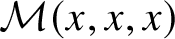
come in either clockwise or counterclockwise order. A constant map
$(T_x L_0,T_x L_1,T_x L_2)$
come in either clockwise or counterclockwise order. A constant map
 $D \to L_0 \cap L_1 \cap L_2$
contributes to
$D \to L_0 \cap L_1 \cap L_2$
contributes to
 $\mathcal {M}(x,x,x)$
if and only if they come in clockwise order:
$\mathcal {M}(x,x,x)$
if and only if they come in clockwise order:

An example of a nontransversely cut quadrilateral in T (necessarily constant) is analyzed in [Reference Lekili and PerutzLPe1, Thm. 8]. We will encounter some nontransversely cut triangles in Subsection 4.9.
2.3 Maslov index of an intersection point
Let
 $(L,L')$
be an ordered pair of connected 1-dimensional submanifolds of T and fix an orientation of both L and
$(L,L')$
be an ordered pair of connected 1-dimensional submanifolds of T and fix an orientation of both L and
 $L'$
. Suppose that L and
$L'$
. Suppose that L and
 $L'$
meet transversely at the point x; then we define
$L'$
meet transversely at the point x; then we define
 $\mathrm {mas}(x) \in \mathbf {Z}/2$
by the rule indicated in the diagram:
$\mathrm {mas}(x) \in \mathbf {Z}/2$
by the rule indicated in the diagram:

If L and
 $L'$
are not homologous to zero, one may lift the Maslov index to a
$L'$
are not homologous to zero, one may lift the Maslov index to a
 $\mathbf {Z}$
-valued invariant by equipping L and
$\mathbf {Z}$
-valued invariant by equipping L and
 $L'$
(and T) with gradings; see [Reference Lekili and PerutzLPe2, §6]. Let us denote this
$L'$
(and T) with gradings; see [Reference Lekili and PerutzLPe2, §6]. Let us denote this
 $\mathbf {Z}$
-valued Maslov index by
$\mathbf {Z}$
-valued Maslov index by
 $\mathrm {mas}_{\mathbf {Z}}(x)$
. A formula for the dimension near
$\mathrm {mas}_{\mathbf {Z}}(x)$
. A formula for the dimension near
 $u \in \mathcal {M}(x_0,\ldots ,x_n)$
is
$u \in \mathcal {M}(x_0,\ldots ,x_n)$
is
 $$ \begin{align} \mathrm{mas}_{\mathbf{Z}}(x_0) - \mathrm{mas}_{\mathbf{Z}}(x_1) - \cdots - \mathrm{mas}_{\mathbf{Z}}(x_n). \end{align} $$
2.4 Sign of a rigid polygon
By making some additional choices, one may attach a sign to each rigid polygon with boundary on
 $(L_0,\ldots ,L_n)$
– in other words, one may define a map
$(L_0,\ldots ,L_n)$
– in other words, one may define a map
 $$ \begin{align} \mathcal{M}(x_0,\ldots,x_n) \to \{1,-1\}. \end{align} $$
We recall the recipe for (2.4.1) given in [Reference SeidelSe1, §7] – it depends on the choice of orientation for each
 $L_i$
and on the additional data of a basepoint
$L_i$
and on the additional data of a basepoint
 $\star _i \in L_i$
in each
$\star _i \in L_i$
in each
 $L_i$
. One requires that
$L_i$
. One requires that
 $\star _i \notin L_j$
for any
$\star _i \notin L_j$
for any
 $j \neq i$
. The point
$j \neq i$
. The point
 $\star _i$
endows
$\star _i$
endows
 $L_i$
with a nontrivial spin structure (also known as bounding or Neveu–Schwarz spin structure) which is trivialised away from
$L_i$
with a nontrivial spin structure (also known as bounding or Neveu–Schwarz spin structure) which is trivialised away from
 $\star _i$
.
$\star _i$
.
If
 $u\vert _{\partial D}:\partial D \to \cup _{i = 0}^n L_i$
preserves the counterclockwise orientation of D, the sign is
$u\vert _{\partial D}:\partial D \to \cup _{i = 0}^n L_i$
preserves the counterclockwise orientation of D, the sign is
 $+1$
or
$+1$
or
 $-1$
according to whether one encounters an even or odd number of stars going around
$-1$
according to whether one encounters an even or odd number of stars going around
 $\partial D$
– that is, it is
$\partial D$
– that is, it is
 $(-1)^{\#u^{-1}\{\star _0,\ldots ,\star _n\}}$
. Changing the orientation of
$(-1)^{\#u^{-1}\{\star _0,\ldots ,\star _n\}}$
. Changing the orientation of
 $L_0$
does not change this sign, changing the orientation of
$L_0$
does not change this sign, changing the orientation of
 $L_n$
changes the signs by
$L_n$
changes the signs by
 $(-1)^{\mathrm {mas}(x_0) + \mathrm {mas}(x_n)}$
and changing the orientation of any of the other
$(-1)^{\mathrm {mas}(x_0) + \mathrm {mas}(x_n)}$
and changing the orientation of any of the other
 $L_i$
changes the sign by
$L_i$
changes the sign by
 $(-1)^{\mathrm {mas}(x_i)}$
.
$(-1)^{\mathrm {mas}(x_i)}$
.
For short, we will sometimes write
 $$ \begin{align} (-1)^{|x|}:=(-1)^{\mathrm{mas}(x)}. \end{align} $$
2.5 Floer cochain complexes
Let t be a formal variable and let
 $\mathbf {Z}[t^{\mathbf {R}_{\geq 0}}]$
denote the semigroup algebra of
$\mathbf {Z}[t^{\mathbf {R}_{\geq 0}}]$
denote the semigroup algebra of
 $\mathbf {R}_{\geq 0}$
; that is, the group of finite
$\mathbf {R}_{\geq 0}$
; that is, the group of finite
 $\mathbf {Z}$
-linear combinations of symbols of the form
$\mathbf {Z}$
-linear combinations of symbols of the form
 $t^a$
, where
$t^a$
, where
 $a \in \mathbf {R}_{\geq 0}$
, with the multiplication
$a \in \mathbf {R}_{\geq 0}$
, with the multiplication
 $t^a t^b = t^{a+b}$
. Let
$t^a t^b = t^{a+b}$
. Let
 $\Lambda $
be a
$\Lambda $
be a
 $\mathbf {Z}[t^{\mathbf {R}_{\geq 0}}]$
-algebra. In a moment we will take
$\mathbf {Z}[t^{\mathbf {R}_{\geq 0}}]$
-algebra. In a moment we will take
 $\Lambda $
to be the Novikov completion of
$\Lambda $
to be the Novikov completion of
 $\mathbf {Z}[t^{\mathbf {R}_{\geq 0}}]$
, but the differential in
$\mathbf {Z}[t^{\mathbf {R}_{\geq 0}}]$
, but the differential in
 $\mathrm {CF}(L,L')$
is given by a finite sum, so that in this section it might as well be
$\mathrm {CF}(L,L')$
is given by a finite sum, so that in this section it might as well be
 $\mathbf {Z}[t^{\mathbf {R}_{\geq 0}}]$
itself.
$\mathbf {Z}[t^{\mathbf {R}_{\geq 0}}]$
itself.
When L and
 $L'$
intersect transversely, then we let
$L'$
intersect transversely, then we let
 $$ \begin{align} \mathrm{CF}(L,L') := \bigoplus_{x \in L \cap L'} \Lambda. \end{align} $$
The choice of orientation for L and
 $L'$
endows this group with a
$L'$
endows this group with a
 $\mathbf {Z}/2$
-grading,
$\mathbf {Z}/2$
-grading,
 $$ \begin{align*} \mathrm{CF} = \mathrm{CF}^0 \oplus \mathrm{CF}^1, \qquad \text{where } \mathrm{CF}^i(L,L') := \bigoplus_{x | \mathrm{mas}(x) = i} \Lambda. \end{align*} $$
Further equipping L and
 $L'$
with stars (Subsection 2.4) gives us the bigon differential
$L'$
with stars (Subsection 2.4) gives us the bigon differential
 $$ \begin{align} \mu_1:\mathrm{CF}^i(L,L') \to \mathrm{CF}^{i+1}(L,L'): x \mapsto \sum_{y \mid \mathrm{mas}(y) = i+1} y \left(\sum_{u \in \mathcal{M}(x,y)} \pm t^{\mathrm{area}(u)}\right) \end{align} $$
where the sign is given in Subsection 2.4 and
 $\mathrm {area}(u):=\int _D u^* (dx\, dy)$
. The inner sum is finite. A general argument using nonrigid bigons shows that
$\mathrm {area}(u):=\int _D u^* (dx\, dy)$
. The inner sum is finite. A general argument using nonrigid bigons shows that
 $\mu _1 \mu _1 = 0$
– this is a case of the
$\mu _1 \mu _1 = 0$
– this is a case of the
 $A_{\infty }$
-relations (Subsection 2.11). In T, this can be proved more simply by lifting the grading from
$A_{\infty }$
-relations (Subsection 2.11). In T, this can be proved more simply by lifting the grading from
 $\mathbf {Z}/2$
to
$\mathbf {Z}/2$
to
 $\mathbf {Z}$
: the
$\mathbf {Z}$
: the
 $\mathbf {Z}$
-grading is always concentrated in only two degrees.
$\mathbf {Z}$
-grading is always concentrated in only two degrees.
We have just described the ‘absolute’ Floer cochain complex. After fixing a point
 $D \in T$
, not on L or
$D \in T$
, not on L or
 $L'$
, we also have a ‘relative to D’ complex in which
$L'$
, we also have a ‘relative to D’ complex in which
 $\Lambda $
in (2.5.1) can be shrunk to
$\Lambda $
in (2.5.1) can be shrunk to
 $\mathbf {Z}[t]$
(or another
$\mathbf {Z}[t]$
(or another
 $\mathbf {Z}[t]$
-algebra) and the expression
$\mathbf {Z}[t]$
-algebra) and the expression
 $t^{\mathrm {area}(u)}$
in is replaced by
$t^{\mathrm {area}(u)}$
in is replaced by
 $t^{\#u^{-1}(D)}$
.
$t^{\#u^{-1}(D)}$
.
2.6 Example – special Lagrangians
We will call a circle
 $L \subset T$
a ‘special Lagrangian’ if it is the image under
$L \subset T$
a ‘special Lagrangian’ if it is the image under
 $\mathbf {R}^2 \to T$
of a straight line. If that straight line has the form
$\mathbf {R}^2 \to T$
of a straight line. If that straight line has the form
 $y+mx = b$
, then we will call m the slope of the special Lagrangian; otherwise, we say L has slope
$y+mx = b$
, then we will call m the slope of the special Lagrangian; otherwise, we say L has slope
 $\infty $
. Thus, the possible slopes are
$\infty $
. Thus, the possible slopes are
 $m \in \mathbf {Q} \cup \{\infty \}$
. If L is special with finite slope, let us call the orientation under the parametrisation
$m \in \mathbf {Q} \cup \{\infty \}$
. If L is special with finite slope, let us call the orientation under the parametrisation
 $x \mapsto (x,b-mx)$
the ‘default orientation’.
$x \mapsto (x,b-mx)$
the ‘default orientation’.
If
 $L \neq L'$
are two special Lagrangians, of finite slopes m and
$L \neq L'$
are two special Lagrangians, of finite slopes m and
 $m'$
, then they meet transversely in a set of cardinality
$m'$
, then they meet transversely in a set of cardinality
 $|nd' - n'd|$
, if
$|nd' - n'd|$
, if
 $m = n/d$
and
$m = n/d$
and
 $m' = n'/d'$
. All of the intersection points are in a single Maslov degree; with the default orientations, these degrees are
$m' = n'/d'$
. All of the intersection points are in a single Maslov degree; with the default orientations, these degrees are
 $$ \begin{align*} \mathrm{CF}(L,L') = \begin{cases} \mathrm{CF}^0(L,L') & \text{if}\ m'> m \\ \mathrm{CF}^1(L,L') & \text{if}\ m' < m. \end{cases} \end{align*} $$
There are no bigons and the differential (2.5.2) is zero.
2.7 Polygon maps
Suppose that
 $(L_0,\ldots ,L_n)$
are in sufficiently general position that all of the
$(L_0,\ldots ,L_n)$
are in sufficiently general position that all of the
 $\mathcal {M}(x_0,\ldots ,x_n)$
are transversely cut. The
$\mathcal {M}(x_0,\ldots ,x_n)$
are transversely cut. The
 $(n+1)$
-gon map is a multilinear map
$(n+1)$
-gon map is a multilinear map
 $$ \begin{align} \mu_n:\mathrm{CF}^{i_n}(L_{n-1},L_n) \times \cdots \times \mathrm{CF}^{i_1}(L_0,L_1) \to \mathrm{CF}^{i_1+\cdots+i_n + 2 - n}(L_0,L_n) \end{align} $$
which carries
 $(x_n,x_{n-1},\ldots ,x_1)$
to
$(x_n,x_{n-1},\ldots ,x_1)$
to
 $$ \begin{align} \sum_{y} y \left(\sum_{u \in \mathcal{M}(y,x_1,x_2,\ldots,x_n)} \pm t^{\mathrm{area}(u)}\right). \end{align} $$
It is not defined until the
 $L_i$
are equipped with orientations and stars. Furthermore, the inner sum in (2.7.2) is usually infinite, so
$L_i$
are equipped with orientations and stars. Furthermore, the inner sum in (2.7.2) is usually infinite, so
 $\Lambda $
should carry a topology in which it converges. The standard choice for
$\Lambda $
should carry a topology in which it converges. The standard choice for
 $\Lambda $
is one of
$\Lambda $
is one of
 $\Lambda ^0$
or
$\Lambda ^0$
or
 $\Lambda ^0[t^{-1}]$
, where
$\Lambda ^0[t^{-1}]$
, where
 $\Lambda ^0$
is the Novikov ring
$\Lambda ^0$
is the Novikov ring
 $$ \begin{align} \Lambda^0 = \Lambda_{\mathbf{Z}}^0 =\left\{\sum_{i = 0}^{\infty} a_i t^{\lambda_i} \mid a_i \in \mathbf{Z}, \lambda_i \in \mathbf{R}_{\geq 0} \text{ and } \lim_{i \to \infty} \lambda_i = \infty\right\}. \end{align} $$
The fact that
 $\Lambda ^0$
can be taken to have
$\Lambda ^0$
can be taken to have
 $\mathbf {Z}$
-coefficients is a reflection of the fact that the moduli spaces
$\mathbf {Z}$
-coefficients is a reflection of the fact that the moduli spaces
 $\mathcal {M}$
are not orbifolds – this holds for T and more generally for semipositive symplectic manifolds.
$\mathcal {M}$
are not orbifolds – this holds for T and more generally for semipositive symplectic manifolds.
In the relative setting, as long as D does not lie on any
 $L_i$
, we replace
$L_i$
, we replace
 $t^{\mathrm {area}(u)}$
with
$t^{\mathrm {area}(u)}$
with
 $t^{\#u^{-1}(D)}$
and (2.7.1) is multilinear over
$t^{\#u^{-1}(D)}$
and (2.7.1) is multilinear over
 $\mathbf {Z}[\![t]\!]$
.
$\mathbf {Z}[\![t]\!]$
.
2.8 Example – some triangle maps
Suppose
 $L_0,\ldots ,L_k$
are special Lagrangians of slopes
$L_0,\ldots ,L_k$
are special Lagrangians of slopes
 $$ \begin{align} m_0 < m_1 < \cdots < m_k < \infty. \end{align} $$
If
 $k \neq 2$
, then the set of rigid
$k \neq 2$
, then the set of rigid
 $(k+1)$
-gons with boundary on
$(k+1)$
-gons with boundary on
 $L_0,\ldots ,L_k$
is empty and the maps
$L_0,\ldots ,L_k$
is empty and the maps
 $$ \begin{align*} \mu_k:\mathrm{CF}(L_{k-1},L_k) \times \cdots \times \mathrm{CF}(L_0,L_1) \to \mathrm{CF}(L_0,L_k) \end{align*} $$
are zero – this is a consequence of Subsection 2.3.1. In other words, when (2.8.1) is satisfied,
 $\mu _2$
is the only interesting polygon map. In this section we explain how to compute
$\mu _2$
is the only interesting polygon map. In this section we explain how to compute
 $\mu _2$
in detail for Lagrangians of the form
$\mu _2$
in detail for Lagrangians of the form
 $L_{(m_0)}, L_{(m_1)},L_{(m_2)}$
(Subsection 1.3). These are the maps that can be packed into a product structure on
$L_{(m_0)}, L_{(m_1)},L_{(m_2)}$
(Subsection 1.3). These are the maps that can be packed into a product structure on
 $\bigoplus \mathrm {CF}(L_{(0)},L_{(m)})$
(Subsection 1.4), and our notation is adapted to describing this product structure.
$\bigoplus \mathrm {CF}(L_{(0)},L_{(m)})$
(Subsection 1.4), and our notation is adapted to describing this product structure.
One consequence of the vanishing of the
 $\mu _k$
for
$\mu _k$
for
 $k \neq 2$
is that this product is strictly associative (Subsection 2.11), and we can describe the product in terms of the theta functions. If (2.8.1) is not satisfied, then the maps
$k \neq 2$
is that this product is strictly associative (Subsection 2.11), and we can describe the product in terms of the theta functions. If (2.8.1) is not satisfied, then the maps
 $\mu _k$
do not all vanish for
$\mu _k$
do not all vanish for
 $k \geq 3$
– they can be written in terms of Hecke’s indefinite theta series [Reference PolishchukPoli].
$k \geq 3$
– they can be written in terms of Hecke’s indefinite theta series [Reference PolishchukPoli].
If
 $m_1 < m_2$
, there are
$m_1 < m_2$
, there are
 $m_2 - m_1$
intersection points between
$m_2 - m_1$
intersection points between
 $L_{(m_1)}$
and
$L_{(m_1)}$
and
 $L_{(m_2)}$
, each contributing a basis element to
$L_{(m_2)}$
, each contributing a basis element to
 $\mathrm {CF}(L_{(m_1)},L_{(m_2)})$
. Let us index those intersection points in the following way:
$\mathrm {CF}(L_{(m_1)},L_{(m_2)})$
. Let us index those intersection points in the following way:
 $$ \begin{align} \tau^{m_1}(x_{m_2 - m_1,\kappa}) := (\kappa,-m_2\kappa) \end{align} $$
where
 $\kappa \in \{0,\frac {1}{m_2 - m_1},\ldots , \frac {m_2 - m_1 - 1}{m_2 - m_1}\}$
and
$\kappa \in \{0,\frac {1}{m_2 - m_1},\ldots , \frac {m_2 - m_1 - 1}{m_2 - m_1}\}$
and
 $\tau $
denotes the Dehn twist map
$\tau $
denotes the Dehn twist map
 $$ \begin{align*} \tau:(x,y) \mapsto (x,y-x) \end{align*} $$
Fix an irrational number
 $\varepsilon $
and equip each
$\varepsilon $
and equip each
 $L_{(m)}$
with a star §2.4
$L_{(m)}$
with a star §2.4
 $$ \begin{align} \star_{(m)} = \star_{(m),\varepsilon} := (\varepsilon,-m\varepsilon). \end{align} $$
The Dehn twist carries
 $L_{(m)}$
to
$L_{(m)}$
to
 $L_{(m+1)}$
and preserves the stars. As
$L_{(m+1)}$
and preserves the stars. As
 $\varepsilon $
is irrational, the stars avoid the intersection points
$\varepsilon $
is irrational, the stars avoid the intersection points
 $L_{(m_1)} \cap L_{(m_2)}$
. We will compute the triangle maps
$L_{(m_1)} \cap L_{(m_2)}$
. We will compute the triangle maps
 $$ \begin{align*} \mathrm{CF}(L_{(m_1)},L_{(m_1+m_2)}) \times \mathrm{CF}(L_{(0)},L_{((m_1))}) \to \mathrm{CF}(L_{(0)},L_{(m_1+m_2)}) \end{align*} $$
by computing
 $\mu _2(\tau ^{m_1} x_{m_2,\kappa _2}, x_{m_1,\kappa _1})$
. For example,
$\mu _2(\tau ^{m_1} x_{m_2,\kappa _2}, x_{m_1,\kappa _1})$
. For example,
 $$ \begin{align} \mu_2(\tau x_{1,0},x_{1,0}) = \begin{cases} x_{2,0}\Big(\sum_{i \in \mathbf{Z}} t^{i^2}\Big) + x_{2,\frac{1}{2}}\Big(\sum_{i \in \mathbf{Z}} t^{(i+\frac{1}{2})^2}\Big) & \text{(absolute setting)} \\ x_{2,0}\Big(\sum_{i \in \mathbf{Z}} t^{i^2}\Big) + x_{2,\frac{1}{2}}\Big(\sum_{i \in \mathbf{Z}} t^{i(i+1)}\Big) & \text{(relative setting)}. \end{cases} \end{align} $$
Theorem. Let
 $$ \begin{align} E(\kappa_1,\kappa_2) = E_{m_1,m_2}(\kappa_1,\kappa_2) := \frac{m_1 \kappa_1 + m_2 \kappa_2}{m_1 + m_2} \end{align} $$
(which carries
 $\frac {1}{m_1} \mathbf {Z} \times \frac {1}{m_2} \mathbf {Z}$
into
$\frac {1}{m_1} \mathbf {Z} \times \frac {1}{m_2} \mathbf {Z}$
into
 $\frac {1}{m_1+m_2} \mathbf {Z}$
). Then in the absolute setting,
$\frac {1}{m_1+m_2} \mathbf {Z}$
). Then in the absolute setting,
 $\mu _2(\tau ^{m_1} x_{m_2,\kappa _2}, x_{m_1,\kappa _1})$
is given by
$\mu _2(\tau ^{m_1} x_{m_2,\kappa _2}, x_{m_1,\kappa _1})$
is given by
 $$ \begin{align} \mu_2(\tau^{m_1} x_{m_2,\kappa_2}, x_{m_1,\kappa_1}) = \sum_{\ell \in \mathbf{Z}} x_{m_1 + m_2,E(\kappa_1,\kappa_2 + \ell)} t^{(\ell+\kappa_2 - \kappa_1)^2/(2(\frac{1}{m_1} + \frac{1}{m_2}))}. \end{align} $$
Let the functions
 $\phi (s)$
and
$\phi (s)$
and
 $\lambda (u,v) = \lambda _{m_1,m_2}(u,v)$
be given by (cf. [Reference Lekili and PerutzLPe2, p. 83])
$\lambda (u,v) = \lambda _{m_1,m_2}(u,v)$
be given by (cf. [Reference Lekili and PerutzLPe2, p. 83])
 $$ \begin{align} \phi(s):= \lfloor s \rfloor s - \frac{1}{2} \lfloor s \rfloor \lfloor s+1 \rfloor; \qquad \lambda(u,v) := m_1 \phi(u) + m_2 \phi(v) - (m_1 + m_2) \phi(E(u,v)). \end{align} $$
Then in the relative setting,
 $\mu _2(\tau ^{m_1} x_{m_2,\kappa _2}, x_{m_1,\kappa _1})$
is given by
$\mu _2(\tau ^{m_1} x_{m_2,\kappa _2}, x_{m_1,\kappa _1})$
is given by
 $$ \begin{align} \mu_2(\tau^{m_1} x_{m_2,.\kappa_2},x_{m_1,\kappa_1}) = \sum_{\ell \in \mathbf{Z}} x_{m_1 + m_2,E(\kappa_1,\kappa_2 + \ell)} t^{\lambda(\kappa_1,\kappa_2+\ell)}, \end{align} $$
where we understand
 $x_{m_1+m_2,E(\kappa _1,\kappa _2+\ell )} := x_{m_1 + m_2,\kappa }$
if
$x_{m_1+m_2,E(\kappa _1,\kappa _2+\ell )} := x_{m_1 + m_2,\kappa }$
if
 $E(\kappa _1,\kappa _2+\ell ) = \kappa $
modulo
$E(\kappa _1,\kappa _2+\ell ) = \kappa $
modulo
 $1$
.
$1$
.
Proof. The index
 $\ell $
in either sum (2.8.6), (2.8.8) determines a triangle, two of whose vertices are at
$\ell $
in either sum (2.8.6), (2.8.8) determines a triangle, two of whose vertices are at
 $x_{m_1,\kappa _1}$
and
$x_{m_1,\kappa _1}$
and
 $\tau ^{m_1} x_{m_2,\kappa _2}$
. In the universal cover, the coordinates of all three vertices are
$\tau ^{m_1} x_{m_2,\kappa _2}$
. In the universal cover, the coordinates of all three vertices are
 $$ \begin{align*} (\kappa_1,0), \qquad (E(\kappa_1,\kappa_2+\ell),0), \qquad (\kappa_2+\ell,-m_1(\kappa_2 + \ell - \kappa_1)) \end{align*} $$
as in the diagram

On any of these triangles there are an even number of stars (2.8.3): for each
 $i \in \mathbf {Z}$
with
$i \in \mathbf {Z}$
with
 $\kappa _1 < \varepsilon + i < \kappa _2 + \ell $
there are exactly two stars whose x-coordinate (in the universal cover) is
$\kappa _1 < \varepsilon + i < \kappa _2 + \ell $
there are exactly two stars whose x-coordinate (in the universal cover) is
 $\varepsilon +i$
, one along
$\varepsilon +i$
, one along
 $L_{(m_1)}$
and the other along either
$L_{(m_1)}$
and the other along either
 $L_{(0)}$
or
$L_{(0)}$
or
 $L_{(m_1+m_2)}$
. Thus, every summand in the triangle has sign
$L_{(m_1+m_2)}$
. Thus, every summand in the triangle has sign
 $+1$
.
$+1$
.
The exponent of t in (2.8.6) is the area of the
 $\ell $
th triangle; that is,
$\ell $
th triangle; that is,
 $$ \begin{align*} \frac{1}{2} m_1(\kappa_2+\ell-\kappa_1) (E(\kappa_1, \kappa_2+\ell) - \kappa_1) =(\ell+\kappa_2-\kappa_1)^2 / (2(\frac{1}{m_1}+\frac{1}{m_2})). \end{align*} $$
The more complicated exponent of t in (2.8.8) is the lattice area (Subsection 1.6) of the same triangle, which coincides with the cardinality of
 $u^{-1}(D)$
when D is in the first quadrant very close to
$u^{-1}(D)$
when D is in the first quadrant very close to
 $(0,0)$
– see [Reference Lekili and PerutzLPe2].
$(0,0)$
– see [Reference Lekili and PerutzLPe2].
2.9 Theta functions
Let
 $\theta _{m,k}$
,
$\theta _{m,k}$
,
 $\theta ^{\mathrm {abs}}_{m,k}$
be as in (1.8.1):
$\theta ^{\mathrm {abs}}_{m,k}$
be as in (1.8.1):
 $$ \begin{align*} \theta_{m,k} := \sum_{i = -\infty}^{\infty} t^{m \frac{i (i-1)}{2}+ k i}\, z^{mi + k}, \qquad \theta^{\mathrm{abs}}_{m,k} := \sum_{i = -\infty}^{\infty} t^{(mi+k)^2/(2m)} z^{mi+k}. \end{align*} $$
The Jacobi theta function is
 $\theta _{1,0}$
and the others are obtained by a simple change of variables:
$\theta _{1,0}$
and the others are obtained by a simple change of variables:
 $$ \begin{align*} \theta_{m,k}(t,z) = z^k \theta_{1,0}(t^m,t^k z^m), \qquad \theta_{m,k}(t,t^{\frac{1}{2}} z) = t^{{k(m-k)}/(2m)}\theta_{m,k}^{\mathrm{abs}}(t,z). \end{align*} $$
Although these series are doubly infinite in z, when formally expanding the product of
 $\theta _{m,k}$
and
$\theta _{m,k}$
and
 $\theta _{m',k'}$
, only finitely many terms contribute to the coefficient of any monomial
$\theta _{m',k'}$
, only finitely many terms contribute to the coefficient of any monomial
 $z^e t^f$
– the same goes for
$z^e t^f$
– the same goes for
 $\theta ^{\mathrm {abs}}_{m,k}$
and
$\theta ^{\mathrm {abs}}_{m,k}$
and
 $\theta ^{\mathrm {abs}}_{m',k'}$
. This is a consequence of the convexity of the functions
$\theta ^{\mathrm {abs}}_{m',k'}$
. This is a consequence of the convexity of the functions
 $i \mapsto m \binom {i}{2}+ki$
and
$i \mapsto m \binom {i}{2}+ki$
and
 $i \mapsto (mi+k)^2/(2m)$
in the exponent of t. That the resulting series
$i \mapsto (mi+k)^2/(2m)$
in the exponent of t. That the resulting series
 $\theta _{m,k} \cdot \theta _{m',k'}$
or
$\theta _{m,k} \cdot \theta _{m',k'}$
or
 $\theta ^{\mathrm {abs}}_{m,k} \cdot \theta ^{\mathrm {abs}}_{m',k'}$
can be written as a linear combination of
$\theta ^{\mathrm {abs}}_{m,k} \cdot \theta ^{\mathrm {abs}}_{m',k'}$
can be written as a linear combination of
 $\theta _{m+m',0},\cdots ,\theta _{m+m',m+m'-1}$
is a standard but nontrivial fact about the theta functions. The formulas for these coefficients are the same as (2.8.8) and (2.8.6): putting
$\theta _{m+m',0},\cdots ,\theta _{m+m',m+m'-1}$
is a standard but nontrivial fact about the theta functions. The formulas for these coefficients are the same as (2.8.8) and (2.8.6): putting
 $\kappa _1 = k_1/m_1$
and
$\kappa _1 = k_1/m_1$
and
 $\kappa _2 = k_2/m_2$
,
$\kappa _2 = k_2/m_2$
,
 $$ \begin{align*} \theta_{m_2,k_2} \cdot \theta_{m_1,k_1} = \sum_{\ell \in \mathbf{Z}} \theta_{m_1 + m_2,E(\kappa_1,\kappa_2 + \ell)} t^{\lambda(\kappa_1,\kappa_2 + \ell)} \end{align*} $$
and
 $$ \begin{align*} \theta^{\mathrm{abs}}_{m_2,k_2} \cdot \theta^{\mathrm{abs}}_{m_1,k_1} = \sum_{\ell \in \mathbf{Z}} \theta^{\mathrm{abs}}_{m_1 + m_2,E(\kappa_1,\kappa_2 + \ell)} t^{(\ell+\kappa_2 - \kappa_1)^2/(2(\frac{1}{m_1} + \frac{1}{m_2}))}. \end{align*} $$
In other words, the map
 $x_{m,k} \mapsto \theta _{m,k}$
or
$x_{m,k} \mapsto \theta _{m,k}$
or
 $\theta ^{\mathrm {abs}}_{m,k}$
is a ring homomorphism. One may verify this directly (and we will do so in the next section when we turn on an F-field), but it is natural to ask what is the Floer-theoretic origin of these series. Each summand of (1.8.1) is indexed by a right triangle, with one vertex at
$\theta ^{\mathrm {abs}}_{m,k}$
is a ring homomorphism. One may verify this directly (and we will do so in the next section when we turn on an F-field), but it is natural to ask what is the Floer-theoretic origin of these series. Each summand of (1.8.1) is indexed by a right triangle, with one vertex at
 $x_{m,k/m}$
and sides along
$x_{m,k/m}$
and sides along
 $L_{(0)},L_{(m)},L_{(\infty )}$
. The exponent of t carries the area (or lattice area) of this right triangle and the exponent of z carries the number of times the vertical edge of the triangle wraps around
$L_{(0)},L_{(m)},L_{(\infty )}$
. The exponent of t carries the area (or lattice area) of this right triangle and the exponent of z carries the number of times the vertical edge of the triangle wraps around
 $L_{(\infty )}$
– this z can be interpreted as the monodromy of a rank 1 local system (Subsection 3.3). For instance, the right triangles contributing to
$L_{(\infty )}$
– this z can be interpreted as the monodromy of a rank 1 local system (Subsection 3.3). For instance, the right triangles contributing to
 $\theta _{2,1}$
have the form (for i positive)
$\theta _{2,1}$
have the form (for i positive)

2.10 The punctured torus, the large complex structure limit
Part of the motivation for relative Floer theory is to make sense of the specialisation
 $t = 0$
in the polygon sums. Setting
$t = 0$
in the polygon sums. Setting
 $t = 0$
has the effect of discarding the polygons that contribute a positive power of t, which in the relative case is the same as discarding the polygons that touch D. One gets the same effect by doing Floer theory for Lagrangians in the punctured torus
$t = 0$
has the effect of discarding the polygons that contribute a positive power of t, which in the relative case is the same as discarding the polygons that touch D. One gets the same effect by doing Floer theory for Lagrangians in the punctured torus
 $T - D$
. When
$T - D$
. When
 $T-D$
is equipped with the right symplectic structure, one with infinite area in a neighbourhood of D, this is called the ‘large volume limit’ of Floer theory.
$T-D$
is equipped with the right symplectic structure, one with infinite area in a neighbourhood of D, this is called the ‘large volume limit’ of Floer theory.
We can treat the Lagrangians
 $L_{(m)}$
as boundary conditions for triangles
$L_{(m)}$
as boundary conditions for triangles
 $u:\Delta ^2 \to T - D$
and sum over them to obtain a map
$u:\Delta ^2 \to T - D$
and sum over them to obtain a map
 $\mu _2$
as before, this time defined on the free
$\mu _2$
as before, this time defined on the free
 $\mathbf {Z}$
-modules spanned by
$\mathbf {Z}$
-modules spanned by
 $L_{(m_1)} \cap L_{(m_2)}$
. For instance,
$L_{(m_1)} \cap L_{(m_2)}$
. For instance,
 $$ \begin{align*} \mu_2(\tau x_{1,0},x_{1,0}) = x_{2,0} + x_{2,1/2} \cdot 2, \end{align*} $$
where
 $x_{2,0}$
comes from a constant map and the two copies of
$x_{2,0}$
comes from a constant map and the two copies of
 $x_{2,1/2}$
come from the two shaded triangles in the figure
$x_{2,1/2}$
come from the two shaded triangles in the figure

We also record
 $$ \begin{align*} \mu_2(\tau^2 x_{1,0},x_{2,0}) & = x_{3,0} + x_{3,1/3} + x_{3,2/3} \\ \mu_2(\tau^2 x_{1,0},x_{2,1/2}) & = x_{3,1/3} + x_{3,2/3} \\ \mu_2(\tau^3 x_{3,1/3},x_{3,2/3}) & = x_{6,3/6} \\ \end{align*} $$
and
 $$ \begin{align*} \mu_2(\tau^4 x_{2,1/2}, \mu_2(\tau^2 x_{2,1/2},x_{2,1/2})) = x_{6,3/6}. \end{align*} $$
If one sets
 $z = x_{1,0}$
,
$z = x_{1,0}$
,
 $x = x_{2,1/2}$
,
$x = x_{2,1/2}$
,
 $y = x_{3,2/3}$
, these equation imply in particular that
$y = x_{3,2/3}$
, these equation imply in particular that
 $$ \begin{align*} y^2 z + x^3 = xyz. \end{align*} $$
This is the equation for a nodal plane cubic curve – the ‘large complex structure limit’ that matches the large volume limit under mirror symmetry.
2.11
$A_{\infty }$
-relations

The moduli spaces
 $\mathcal {M}$
that parametrise nonrigid polygons are not usually compact. For example, suppose
$\mathcal {M}$
that parametrise nonrigid polygons are not usually compact. For example, suppose
 $L_0,L_1,L_2,L_3$
are as in the diagram
$L_0,L_1,L_2,L_3$
are as in the diagram

Denote the red-black, black-purple and purple-blue intersection points by f, g and h respectively and the blue-red intersection point by
 $hgf$
. Then
$hgf$
. Then
 $\mathcal {M}(hgf,f,g,h)$
includes the following one-parameter family of quadrilaterals:
$\mathcal {M}(hgf,f,g,h)$
includes the following one-parameter family of quadrilaterals:

They all have the same image closure but along the boundary may back-track along either the blue or the red line. Near the
 $\ast $
s, the map u is biholomorphic to the map from the upper half-plane to
$\ast $
s, the map u is biholomorphic to the map from the upper half-plane to
 $\mathbf {C}$
that sends z to
$\mathbf {C}$
that sends z to
 $z^2$
. At the extreme parameters, where the
$z^2$
. At the extreme parameters, where the
 $\ast $
reaches all the way to the black or purple line, there is no such J-holomorphic quadrilateral – so
$\ast $
reaches all the way to the black or purple line, there is no such J-holomorphic quadrilateral – so
 $\mathcal {M}$
is not compact – but each of those extremes is occupied by a pair of J-holomorphic triangles.
$\mathcal {M}$
is not compact – but each of those extremes is occupied by a pair of J-holomorphic triangles.
Since the quadrilaterals are not rigid, they do not contribute to
 $\mu _3(h,g,f)$
. But the triangles at the extremes are rigid; at one end they contribute to
$\mu _3(h,g,f)$
. But the triangles at the extremes are rigid; at one end they contribute to
 $\mu _2(g,f)$
and
$\mu _2(g,f)$
and
 $\mu _2(h,gf)$
and at the other end to
$\mu _2(h,gf)$
and at the other end to
 $\mu _2(h,g)$
and
$\mu _2(h,g)$
and
 $\mu _2(hg,f)$
. The interpolating family of quadrilaterals exhibits a relation between them.
$\mu _2(hg,f)$
. The interpolating family of quadrilaterals exhibits a relation between them.
More generally, there is a compactification (the Deligne–Mumford–Stasheff compactification) of
 $\mathcal {M}$
. When everything is transversely cut (Subsection 2.2), the compactification is a topological manifold-with-corners whose corners are indexed by tuples of rigid polygons. Equipping the
$\mathcal {M}$
. When everything is transversely cut (Subsection 2.2), the compactification is a topological manifold-with-corners whose corners are indexed by tuples of rigid polygons. Equipping the
 $L_i$
with orientations and stars induces an orientation on
$L_i$
with orientations and stars induces an orientation on
 $\mathcal {M}$
and its compactification – (2.4.1) is a special case of this orientation. The oriented compactification of
$\mathcal {M}$
and its compactification – (2.4.1) is a special case of this orientation. The oriented compactification of
 $\mathcal {M}$
is used in the proof (it essentially is the proof) of the following equations among the polygon maps
$\mathcal {M}$
is used in the proof (it essentially is the proof) of the following equations among the polygon maps
 $\mu _n$
:
$\mu _n$
:
 $$ \begin{align} \sum_{i+j = n+1} \sum_{\ell < i} (-1)^{|f_1|+\cdots+|f_\ell|-\ell} \mu_i(f_n,,\ldots,f_{\ell + j + 1},\mu_j(f_{\ell+j},\ldots,f_{\ell+1}),f_{\ell},\ldots,f_1) = 0. \end{align} $$
The algebraic structure formed by the
 $\mathrm {CF}(L,L')$
and the maps
$\mathrm {CF}(L,L')$
and the maps
 $\mu _n$
, subject to the relations (2.11.2), is called an ‘
$\mu _n$
, subject to the relations (2.11.2), is called an ‘
 $A_{\infty }$
-precategory’ in [Reference Kontsevich and SoibelmanKS, §4.3]. Each L is like an object and each
$A_{\infty }$
-precategory’ in [Reference Kontsevich and SoibelmanKS, §4.3]. Each L is like an object and each
 $f \in \mathrm {CF}(L,L')$
is like a morphism between objects. (2.11.2) expresses the fact that these morphism spaces are cochain complexes and that the composition law is associative up to chain homotopy in a strong sense. It falls short of being an
$f \in \mathrm {CF}(L,L')$
is like a morphism between objects. (2.11.2) expresses the fact that these morphism spaces are cochain complexes and that the composition law is associative up to chain homotopy in a strong sense. It falls short of being an
 $A_{\infty }$
-category; for instance, because
$A_{\infty }$
-category; for instance, because
 $\mathrm {CF}(L,L')$
is defined only when L and
$\mathrm {CF}(L,L')$
is defined only when L and
 $L'$
meet transversely, so
$L'$
meet transversely, so
 $\mathrm {CF}(L,L)$
is undefined and there is no ‘morphism’ that could play the role of the identity map. A standard way to address this problem is by analysing the sense in which
$\mathrm {CF}(L,L)$
is undefined and there is no ‘morphism’ that could play the role of the identity map. A standard way to address this problem is by analysing the sense in which
 $\mathrm {CF}(L,L')$
are invariant under Hamiltonian isotopies – Floer’s theory of continuation.
$\mathrm {CF}(L,L')$
are invariant under Hamiltonian isotopies – Floer’s theory of continuation.
2.12 Example – identity maps
There is a Floer cochain complex
 $\mathrm {CF}(L,L')$
, well-defined up to quasi-isomorphism, even if L and
$\mathrm {CF}(L,L')$
, well-defined up to quasi-isomorphism, even if L and
 $L'$
do not intersect transversely. In case
$L'$
do not intersect transversely. In case
 $L'$
meets both
$L'$
meets both
 $L_0$
and
$L_0$
and
 $L_1$
transversely, in the absolute setting (respectively relative setting) any Hamiltonian isotopy (respectively any Hamiltonian isotopy supported on the complement of D) induces a quasi-isomorphism between
$L_1$
transversely, in the absolute setting (respectively relative setting) any Hamiltonian isotopy (respectively any Hamiltonian isotopy supported on the complement of D) induces a quasi-isomorphism between
 $\mathrm {CF}(L_0,L')$
and
$\mathrm {CF}(L_0,L')$
and
 $\mathrm {CF}(L_1,L')$
(Subsection 2.13). One accesses
$\mathrm {CF}(L_1,L')$
(Subsection 2.13). One accesses
 $\mathrm {CF}(L,L')$
by perturbing L.
$\mathrm {CF}(L,L')$
by perturbing L.
We illustrate this in an example that fills in the zeroth graded piece of (1.4.1). Let
 $\phi ^s$
denote the flow of
$\phi ^s$
denote the flow of
 $H(x,y) = \sin (2 \pi x)$
; that is,
$H(x,y) = \sin (2 \pi x)$
; that is,
 $$ \begin{align} \phi^s(x,y) = (x,y - s \cos(2\pi x)). \end{align} $$
Then for
 $0 < s < 1$
,
$0 < s < 1$
,
 $\phi ^s L_{(0)}$
meets
$\phi ^s L_{(0)}$
meets
 $L_{(0)}$
transversely at the points
$L_{(0)}$
transversely at the points
 $x = (.25,0)$
and
$x = (.25,0)$
and
 $y = (.75,0)$
, so that
$y = (.75,0)$
, so that
 $\mathrm {CF}(\phi ^s L_{(0)},L_{(0)}) = \Lambda x \oplus \Lambda y$
. In a suitable fundamental domain, the picture is this:
$\mathrm {CF}(\phi ^s L_{(0)},L_{(0)}) = \Lambda x \oplus \Lambda y$
. In a suitable fundamental domain, the picture is this:

Equipping
 $L_{(0)}$
with its default orientation and
$L_{(0)}$
with its default orientation and
 $\phi ^s L_{(0)}$
with the orientation induced by
$\phi ^s L_{(0)}$
with the orientation induced by
 $\phi ^s:L_{(0)} \cong \phi ^s L_{(0)}$
, the Maslov degrees are
$\phi ^s:L_{(0)} \cong \phi ^s L_{(0)}$
, the Maslov degrees are
 $$ \begin{align} \mathrm{CF}^0(\phi^s L_{(0)},L_{(0)}) = x \Lambda \qquad \mathrm{CF}^1(\phi^s L_{(0)},L_{(0)}) = y\Lambda. \end{align} $$
There are two bigons contributing to the differential
 $\mu _1$
, of equal area A. Both bigons have input x and output y and their signs (Subsection 2.4) are opposite to each other (no matter where the stars are placed), so that the differential is
$\mu _1$
, of equal area A. Both bigons have input x and output y and their signs (Subsection 2.4) are opposite to each other (no matter where the stars are placed), so that the differential is
 $$ \begin{align*} \mu_1(x) = y(t^A - t^A) = 0. \end{align*} $$
Some variations of this computation are made in Subsection 2.14 and Subsection 3.5.
2.13 Continuation
Let
 $X_H$
denote the Hamiltonian vector field of a function
$X_H$
denote the Hamiltonian vector field of a function
 $H:[0,1] \times T \to \mathbf {R}$
and write
$H:[0,1] \times T \to \mathbf {R}$
and write
 $\phi ^s$
for its time s flow,
$\phi ^s$
for its time s flow,
 $\phi ^s:T \to T$
. Let us review how the quasi-isomorphism
$\phi ^s:T \to T$
. Let us review how the quasi-isomorphism
 $$ \begin{align} \mathrm{CF}(L,L') \to \mathrm{CF}(\phi^s L, L') \end{align} $$
works in the absolute setting. The map (2.13.1) goes back to [Reference FloerFl, Thm. 4]; our notation is closer to the appendix of [Reference AurouxAur1]. It is defined in terms of a set
 $\mathcal {M}(x,y,\phi ,\beta )$
of maps
$\mathcal {M}(x,y,\phi ,\beta )$
of maps
 $$ \begin{align*} u:[-\infty,\infty] \times [0,1] \to T \end{align*} $$
that obey the boundary conditions
 $$ \begin{align*} \begin{array}{rcl} u([-\infty,\infty] \times \{0\}) & \subset & L \\ \quad u([-\infty,\infty] \times \{1\}) & \subset & L' \end{array} \qquad u(\{\infty\} \times [0,1]) = \{x\} \qquad u(-\infty,\tau) = \phi^{s \cdot \tau}(y) \end{align*} $$
and (with analytic index zero; Subsection 2.2) Floer’s
 $X_H$
-perturbed J-holomorphic curve equation:
$X_H$
-perturbed J-holomorphic curve equation:
 $$ \begin{align} \partial u/\partial \sigma + J(\partial u/\partial \tau - \beta(\sigma) s X_H) = 0. \end{align} $$
Here
 $\beta $
(the ‘profile function’) is a monotone decreasing
$\beta $
(the ‘profile function’) is a monotone decreasing
 $\mathbf {R}$
-valued function on
$\mathbf {R}$
-valued function on
 $[-\infty ,\infty ]$
with
$[-\infty ,\infty ]$
with
 $\beta (\sigma ) = 1$
for
$\beta (\sigma ) = 1$
for
 $\sigma \ll 0$
and
$\sigma \ll 0$
and
 $\beta (\sigma ) = 0$
for
$\beta (\sigma ) = 0$
for
 $\sigma \gg 0$
. The formula for (2.13.1) is
$\sigma \gg 0$
. The formula for (2.13.1) is
 $$ \begin{align} x \mapsto \sum_{y \in \phi^s L \cap L'} y \sum_{u \in \mathcal{M}(x,y,\phi)} \pm t^{\text{topological energy of}\ u} \end{align} $$
where the ‘topological energy’ is (see Lemma 14.4.5 [Reference OhOh])
 $$ \begin{align*} \int u^* \omega + \int_{0}^{1} H(\tau, u(\infty, \tau)) d\tau - \int_{-\infty}^{\infty} \beta'(\sigma) s \int_0^1 (H_\tau \circ u) d\tau d\sigma. \end{align*} $$
This is sometimes a negative quantity, so we must allow
 $t^{-1} \in \Lambda $
.
$t^{-1} \in \Lambda $
.
The homotopy inverse to (2.13.1) is just the continuation map for the reversed flow
 $\phi ^{-s}$
. To describe the chain homotopy between the composite
$\phi ^{-s}$
. To describe the chain homotopy between the composite
 $$ \begin{align} \mathrm{CF}(\phi^s L,L') \to \mathrm{CF}(\phi^{-s} \phi^s L,L') = \mathrm{CF}(L,L') \to \mathrm{CF}(\phi^s L,L') \end{align} $$
and the identity map, let
 $B_r(\sigma )$
(for each
$B_r(\sigma )$
(for each
 $r> 0$
) be a function that vanishes on an interval of length r and that agrees up to translation of
$r> 0$
) be a function that vanishes on an interval of length r and that agrees up to translation of
 $\sigma $
with
$\sigma $
with
 $\beta (\sigma )$
when
$\beta (\sigma )$
when
 $\sigma $
is to the left of that interval and with
$\sigma $
is to the left of that interval and with
 $\beta (-\sigma )$
when
$\beta (-\sigma )$
when
 $\sigma $
is to the right of that interval. Then
$\sigma $
is to the right of that interval. Then
 $$ \begin{align} \Delta(y) = \sum_x x \sum_u \pm t^{\text{topological energy of}\ u}, \end{align} $$
where the inner sum is over strips
 $u:[-\infty ,\infty ] \times [0,1] \to T$
that solve (for some r, with index
$u:[-\infty ,\infty ] \times [0,1] \to T$
that solve (for some r, with index
 $-1$
)
$-1$
)
 $$ \begin{align*} \partial u/\partial \sigma + J(\partial u/\partial \tau - B_r(\sigma) s X_H) = 0 \qquad r \in \mathbf{R}_{\geq 0} \end{align*} $$
and that have
 $u(-,0) \subset L$
,
$u(-,0) \subset L$
,
 $u(-,1) \subset L'$
and
$u(-,1) \subset L'$
and
 $u(-\infty ,\tau ) = \phi ^{s\cdot \tau }(x)$
and
$u(-\infty ,\tau ) = \phi ^{s\cdot \tau }(x)$
and
 $u(\infty ,\tau ) = \phi ^{s\cdot \tau }(y)$
.
$u(\infty ,\tau ) = \phi ^{s\cdot \tau }(y)$
.
2.14 Example
Suppose that L and
 $L'$
are a pair of parallel, horizontal circles, at distance c apart. With
$L'$
are a pair of parallel, horizontal circles, at distance c apart. With
 $\phi ^s$
as in (2.12.1),
$\phi ^s$
as in (2.12.1),
 $\phi ^s(L) \cap L'$
is empty unless
$\phi ^s(L) \cap L'$
is empty unless
 $|s|> c$
. If
$|s|> c$
. If
 $|s|$
only slightly exceeds c, then
$|s|$
only slightly exceeds c, then
 $\phi ^s(L) \cap L'$
has two intersection points, say, x and y, as in the diagram:
$\phi ^s(L) \cap L'$
has two intersection points, say, x and y, as in the diagram:

Thus,
 $\mathrm {CF}(L,L') = 0$
, while (noting that there are two bigons in the right picture, a small one of area A and a large one of area
$\mathrm {CF}(L,L') = 0$
, while (noting that there are two bigons in the right picture, a small one of area A and a large one of area
 $A+c$
) and
$A+c$
) and
 $\mathrm {CF}(\phi ^s L, L') = x \Lambda \oplus y\Lambda $
, with differential
$\mathrm {CF}(\phi ^s L, L') = x \Lambda \oplus y\Lambda $
, with differential
 $$ \begin{align*} \mu_1(x) = y (t^{A} - t^{A+c}) \end{align*} $$
(see Subsection 2.4 for the signs).
As
 $\mathrm {CF}(L,L') = 0$
, the composite (2.13.4) is zero. By Floer’s theorem, the identity map on
$\mathrm {CF}(L,L') = 0$
, the composite (2.13.4) is zero. By Floer’s theorem, the identity map on
 $\mathrm {CF}(\phi ^s L,L')$
is chain homotopic to zero, with (2.13.5) supplying the contracting homotopy. Indeed, the contracting homotopy is the geometric series
$\mathrm {CF}(\phi ^s L,L')$
is chain homotopic to zero, with (2.13.5) supplying the contracting homotopy. Indeed, the contracting homotopy is the geometric series
 $$ \begin{align*} \Delta(y) = x \cdot (t^{-A} + t^{-A + c} + \cdots + t^{-A + nc} + \cdots). \end{align*} $$
The strip
 $u_n$
contributing the nth term in the series (of topological energy
$u_n$
contributing the nth term in the series (of topological energy
 $nc - A$
) stretches horizontally across
$nc - A$
) stretches horizontally across
 $n+2$
fundamental domains, crossing the boundary of the fundamental domain exactly
$n+2$
fundamental domains, crossing the boundary of the fundamental domain exactly
 $n+1$
times. Here is a picture of
$n+1$
times. Here is a picture of
 $u_0\vert _{\partial ([-\infty ,\infty ] \times [0,1])}$
and
$u_0\vert _{\partial ([-\infty ,\infty ] \times [0,1])}$
and
 $u_1\vert _{\partial ([-\infty ,\infty ] \times [0,1])}$
:
$u_1\vert _{\partial ([-\infty ,\infty ] \times [0,1])}$
:

3 Floer theory coupled to an F-field
In this section, we go over the constructions and calculations of Section 2, coupling all of the sums over polygons to a sheaf of rings
 $\underline {\Lambda }$
of the kind discussed in Subsection 1.10. We are interested in the case when
$\underline {\Lambda }$
of the kind discussed in Subsection 1.10. We are interested in the case when
 $\underline {\Lambda }$
is pulled back along the projection map
$\underline {\Lambda }$
is pulled back along the projection map
 $\mathfrak {f}:T \to S^1$
(1.10.2) and set up some notation for dealing with that case in Subsection 3.4.
$\mathfrak {f}:T \to S^1$
(1.10.2) and set up some notation for dealing with that case in Subsection 3.4.
3.1 Cochain complex
If L and
 $L'$
are two embedded circles in T, meeting transversely, let us write (just as in (1.11.1))
$L'$
are two embedded circles in T, meeting transversely, let us write (just as in (1.11.1))
 $$ \begin{align} \mathrm{CF}(L,L';\underline{\Lambda}) := \bigoplus_{x \in L \cap L'} \underline{\Lambda}_x. \end{align} $$
If
 $a \in \underline {\Lambda }_x$
and we wish to regard it as an element of (3.1.1), we will write it as
$a \in \underline {\Lambda }_x$
and we wish to regard it as an element of (3.1.1), we will write it as
 $x \cdot a$
. We equip (3.1.1) with a
$x \cdot a$
. We equip (3.1.1) with a
 $\mathbf {Z}/2$
-grading by equipping L and
$\mathbf {Z}/2$
-grading by equipping L and
 $L'$
with orientations, just as in Subsection 2.5. After further equipping L and
$L'$
with orientations, just as in Subsection 2.5. After further equipping L and
 $L'$
with stars, we define a differential
$L'$
with stars, we define a differential
 $$ \begin{align*} \mu_1:\mathrm{CF}^i(L,L';\underline{\Lambda}) \to \mathrm{CF}^{i+1}(L,L';\underline{\Lambda}) \end{align*} $$
by the following analog of (2.5.2):
 $$ \begin{align} x\cdot a \mapsto \sum_{y | \mathrm{mas}(y) = i+1} y \left(\sum_{u \in \mathcal{M}(y,x)} \pm t^{\mathrm{area}(u)} \nabla \gamma'\left(a \nabla \gamma(1_{\underline{\Lambda}_y})\right)\right), \end{align} $$
where
-
•
$\gamma :I \to L$
is the path along the L-side of the bigon u starting at y and ending at x, -
•
$\gamma ':I \to L'$
is the path along the
$L'$
-side of u starting at x and ending at y.


This differential does not obey anything like
 $\mu _1(xa ) = \mu _1(x)a$
– in fact,
$\mu _1(xa ) = \mu _1(x)a$
– in fact,
 $ \mu _1(x)a$
is typically undefined and, in general,
$ \mu _1(x)a$
is typically undefined and, in general,
 $\mu _1(x a)$
and
$\mu _1(x a)$
and
 $\mu _1(x)$
do not have any useful relationship with each other.
$\mu _1(x)$
do not have any useful relationship with each other.
We obtain a
 $\underline {\Lambda }$
-version of the continuation map (2.13.1)
$\underline {\Lambda }$
-version of the continuation map (2.13.1)
 $$ \begin{align} \mathrm{CF}(L,L';\underline{\Lambda}) \to \mathrm{CF}(\phi^s L,L';\underline{\Lambda}) \end{align} $$
by multiplying each summand of (2.13.3) by
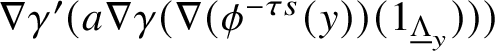 $\nabla \gamma '(a \nabla \gamma (\nabla (\phi ^{-\tau s}(y))(1_{\underline {\Lambda }_y})))$
, where
$\nabla \gamma '(a \nabla \gamma (\nabla (\phi ^{-\tau s}(y))(1_{\underline {\Lambda }_y})))$
, where
 $\gamma = u(\tau ,0)$
and
$\gamma = u(\tau ,0)$
and
 $\gamma ' = u(-\tau ,1)$
are the paths along L and
$\gamma ' = u(-\tau ,1)$
are the paths along L and
 $L'$
respectively and
$L'$
respectively and
 $\phi ^{-\tau s}(y)$
is the reverse of the trajectory from y to
$\phi ^{-\tau s}(y)$
is the reverse of the trajectory from y to
 $\phi ^s y$
; that is,
$\phi ^s y$
; that is,
 $$ \begin{align} \sum_{y \in \phi^s L \cap L'} y \sum_{u \in \mathcal{M}(x,y,\phi)} \pm t^{\text{topological energy of}\ u} \nabla \gamma'(a \nabla \gamma(\nabla (\phi^{-\tau s}(y))(1_{\underline{\Lambda}_y}))). \end{align} $$
The same recipe as Subsection 2.13 gives the homotopy inverse to (3.1.3), only replacing (2.13.5) by
 $$ \begin{align} a \cdot y \mapsto \sum_x x \sum_u \pm t^{\text{topological energy of}\ u} \nabla \gamma' \left(a \cdot \nabla (\phi^{\tau s} (y)) \nabla \gamma \nabla(\phi^{-\tau s}(x)) (1_{\underline{\Lambda}_x})\right). \end{align} $$
3.2 Polygon maps
Let
 $L_0,L_1,\ldots ,L_n$
be oriented, starred submanifolds of T as in Subsection 2.7. We define a variant of (2.7.1)
$L_0,L_1,\ldots ,L_n$
be oriented, starred submanifolds of T as in Subsection 2.7. We define a variant of (2.7.1)
 $$ \begin{align} \mu_n:\mathrm{CF}^{i_n}(L_{n-1},L_n;\underline{\Lambda}) \times \cdots \times \mathrm{CF}^{i_1}(L_0,L_1;\underline{\Lambda}) \to \mathrm{CF}^{i_1+\cdots+i_n + 2 - n}(L_0,L_n;\underline{\Lambda}) \end{align} $$
carrying
 $(x_n \cdot a_n,x_{n-1} \cdot a_{n-1},\ldots , x_1 \cdot a_1)$
(with each
$(x_n \cdot a_n,x_{n-1} \cdot a_{n-1},\ldots , x_1 \cdot a_1)$
(with each
 $a_i \in \underline {\Lambda }_{x_i}$
) to
$a_i \in \underline {\Lambda }_{x_i}$
) to
 $$ \begin{align} \sum_y y \left(\sum_u \pm t^{\mathrm{area}(u)} \nabla \gamma_n(a_n \nabla \gamma_{n-1} (a_{n-1} \cdots \nabla \gamma_2(a_2 \nabla \gamma_1(a_1\nabla(\gamma_0(1))\cdots))))\right), \end{align} $$
where u runs over the same set of rigid polygons as (2.7.1), the signs are just the same and
 $\gamma _i$
is the path along the boundary of u going from
$\gamma _i$
is the path along the boundary of u going from
 $x_i$
to
$x_i$
to
 $x_{i+1}$
or from
$x_{i+1}$
or from
 $x_{n-1}$
to
$x_{n-1}$
to
 $x_0$
.
$x_0$
.
Each connected component of the Deligne–Mumford–Stasheff compactification of the space of nonrigid polygons has the same vertices
 $x_0,\ldots ,x_n$
– that is, every u in that component has those same vertices. Moreover, the path from
$x_0,\ldots ,x_n$
– that is, every u in that component has those same vertices. Moreover, the path from
 $x_i$
to
$x_i$
to
 $x_{i+1}$
or from
$x_{i+1}$
or from
 $x_n$
to
$x_n$
to
 $x_0$
along u belongs to the same homotopy class, so that
$x_0$
along u belongs to the same homotopy class, so that
 $\nabla (\gamma _i):\Lambda _{x_i} \to \Lambda _{x_{i+1}}$
is locally constant in u. Thus, the
$\nabla (\gamma _i):\Lambda _{x_i} \to \Lambda _{x_{i+1}}$
is locally constant in u. Thus, the
 $A_{\infty }$
-relations among the (3.2.1) hold for the usual reasons:
$A_{\infty }$
-relations among the (3.2.1) hold for the usual reasons:
 $$ \begin{align} \sum_{i+j = n+1} \sum_{\ell < i} (-1)^{|x_1| + \cdots+ |x_{\ell}| - \ell} \mu_i(x_n a_n,\ldots, x_{\ell+j+1}a_{\ell+j+1},\mu_j(\cdots), x_\ell a_\ell,\ldots x_1 a_1) = 0. \end{align} $$
3.3 Local systems
We can put the formulas in Subsection 3.2 in context by considering local systems on the
 $L_i$
. For each i, let
$L_i$
. For each i, let
 $\mathcal {E}_i$
be a local system of
$\mathcal {E}_i$
be a local system of
 $\underline {\Lambda }\vert _{L_i}$
-modules on
$\underline {\Lambda }\vert _{L_i}$
-modules on
 $L_i$
. Then we define
$L_i$
. Then we define
 $$ \begin{align} \mathrm{CF}((L_i,\mathcal{E}_i),(L_{i+1},\mathcal{E}_{i+1});\underline{\Lambda}) = \bigoplus_{x \in L_i \cap L_{i+1}} \operatorname{Hom}(\mathcal{E}_{i,x},\mathcal{E}_{i+1,x}). \end{align} $$
The differential is modified by
 $$ \begin{align} \mu_1(xf:\mathcal{E}_{i,x} \to \mathcal{E}_{i+1,x}) = \sum y \sum_u \pm t^{\mathrm{area}(u)} \nabla \gamma' \circ f \circ \nabla \gamma \end{align} $$
(where
 $xf$
denotes f placed in the xth summand of (3.3.1)). In case
$xf$
denotes f placed in the xth summand of (3.3.1)). In case
 $\mathcal {E}_i = \underline {\Lambda }\vert _{L_i}$
is the trivial sheaf of modules, then
$\mathcal {E}_i = \underline {\Lambda }\vert _{L_i}$
is the trivial sheaf of modules, then
 $\operatorname {Hom}(\mathcal {E}_{i,x},\mathcal {E}_{i+1,x}) = \operatorname {Hom}(\underline {\Lambda }_x,\underline {\Lambda }_x)$
is naturally identified with
$\operatorname {Hom}(\mathcal {E}_{i,x},\mathcal {E}_{i+1,x}) = \operatorname {Hom}(\underline {\Lambda }_x,\underline {\Lambda }_x)$
is naturally identified with
 $\underline {\Lambda }_x$
and (3.3.2) coincides with (3.1.2).
$\underline {\Lambda }_x$
and (3.3.2) coincides with (3.1.2).
The polygon maps
 $$ \begin{align} &\mu_n:\mathrm{CF}((L_{n-1},\mathcal{E}_{n-1}),(L_n,\mathcal{E}_n);\underline{\Lambda}) \times \cdots \times \mathrm{CF}((L_0,\mathcal{E}_0),(L_1,\mathcal{E}_1);\underline{\Lambda}) \nonumber\\ &\qquad\qquad\qquad\qquad\qquad\qquad\qquad\qquad\qquad\qquad\qquad\to \mathrm{CF}((L_0,\mathcal{E}_0),(L_n,\mathcal{E}_n);\underline{\Lambda}) \end{align} $$
are defined by sending
 $(f_n,f_{n-1},\ldots ,f_1)$
to the formal expression
$(f_n,f_{n-1},\ldots ,f_1)$
to the formal expression
 $$ \begin{align} \sum_{y} y \left(\sum_{u \in \mathcal{M}(y,x_1,x_2,\ldots,x_n)} \pm t^{\mathrm{area}(u)}\nabla \gamma_n\circ f_n\circ \nabla\gamma_{n-1} \circ f_{n-1} \circ \cdots \circ \nabla \gamma_1 \circ f_1 \circ \nabla \gamma_0 \right). \end{align} $$
We have left the degrees in (3.3.3) off for typesetting reasons; they are the same as in (2.7.1). The formula (3.3.4) specialises to (3.2.2) in case
 $\mathcal {E}_i = \underline {\Lambda }\vert _{L_i}$
. In general, (3.3.4) can fail to converge, unless the following ‘unitarity’ condition is imposed on the
$\mathcal {E}_i = \underline {\Lambda }\vert _{L_i}$
. In general, (3.3.4) can fail to converge, unless the following ‘unitarity’ condition is imposed on the
 $\mathcal {E}_i$
:
$\mathcal {E}_i$
:
Each fibre of
 $\mathcal {E}_i$
is locally free of finite rank over
$\mathcal {E}_i$
is locally free of finite rank over
 $\underline {\Lambda }\vert _{L_i}$
and the monodromy preserves an
$\underline {\Lambda }\vert _{L_i}$
and the monodromy preserves an
 $\underline {\Lambda }^0\vert _{L_i}$
-lattice.
$\underline {\Lambda }^0\vert _{L_i}$
-lattice.
3.4 F-field
We would like to package the
 $\underline {\Lambda }$
-coupled triangle products among the
$\underline {\Lambda }$
-coupled triangle products among the
 $L_{(m)}$
into a graded ring, as in Subsection 1.4. The necessary natural isomorphism between
$L_{(m)}$
into a graded ring, as in Subsection 1.4. The necessary natural isomorphism between
 $\mathrm {CF}(L_{(m)},L_{(n)};\underline {\Lambda })$
and
$\mathrm {CF}(L_{(m)},L_{(n)};\underline {\Lambda })$
and
 $\mathrm {CF}(L_{(0)},L_{(n-m)};\underline {\Lambda })$
exists only when
$\mathrm {CF}(L_{(0)},L_{(n-m)};\underline {\Lambda })$
exists only when
 $\underline {\Lambda }$
is pulled back along the projection map
$\underline {\Lambda }$
is pulled back along the projection map
 $$ \begin{align} \mathfrak{f}:T \to S^1 :(x,y) + \mathbf{Z}^2 \mapsto x + \mathbf{Z}. \end{align} $$
To make this explicit, let
 $\sigma :C \to C$
be a ring automorphism, where C is commutative. We also let
$\sigma :C \to C$
be a ring automorphism, where C is commutative. We also let
 $\sigma $
denote induced automorphism of
$\sigma $
denote induced automorphism of
 $C[\![t]\!]$
or of
$C[\![t]\!]$
or of
 $\Lambda _C$
, with
$\Lambda _C$
, with
 $\sigma (t^a) = t^a$
. We are mainly interested in the case that
$\sigma (t^a) = t^a$
. We are mainly interested in the case that
 $$ \begin{align} C\ \text{perfect of characteristic}\ p, \quad \sigma(c) = c^{1/p}, \end{align} $$
in which case, if
 $f(t) = \sum c_a t^a$
belongs to
$f(t) = \sum c_a t^a$
belongs to
 $C[\![t]\!]$
or to
$C[\![t]\!]$
or to
 $\Lambda _C$
, then we can write
$\Lambda _C$
, then we can write
 $\sigma (f)(t) = f(t^p)^{1/p}$
. The quotient
$\sigma (f)(t) = f(t^p)^{1/p}$
. The quotient
 $$ \begin{align} (\mathbf{R} \times C)/\sim \end{align} $$
of
 $\mathbf {R} \times C$
by the equivalence relation
$\mathbf {R} \times C$
by the equivalence relation
 $(x,c) \sim (x+1,\sigma (c))$
is the étalé space of a locally constant sheaf of rings on
$(x,c) \sim (x+1,\sigma (c))$
is the étalé space of a locally constant sheaf of rings on
 $S^1$
– as are
$S^1$
– as are
 $(\mathbf {R} \times C[\![t]\!])/\sim $
and
$(\mathbf {R} \times C[\![t]\!])/\sim $
and
 $(\mathbf {R} \times \Lambda _C)/\sim $
. We denote the pullback-to-T of these sheaves of rings by
$(\mathbf {R} \times \Lambda _C)/\sim $
. We denote the pullback-to-T of these sheaves of rings by
 $\underline {C}$
,
$\underline {C}$
,
 $\underline {C}[\![t]\!]$
and
$\underline {C}[\![t]\!]$
and
 $\Lambda _{\underline {C}}$
.
$\Lambda _{\underline {C}}$
.
We will call (3.4.1) an ‘F-field’ on T. In diagrams, we keep track of it with a red line – the inverse image of a point close to the right edge of the fundamental domain
 $[0,1)$
of
$[0,1)$
of
 $S^1$
, as in the figure on the left below. On the right we have drawn, in a different scale, the preimage of the red line in part of the universal cover of T, along with a triangle that contributes to
$S^1$
, as in the figure on the left below. On the right we have drawn, in a different scale, the preimage of the red line in part of the universal cover of T, along with a triangle that contributes to
 $\mu _2(x_2 \cdot b,x_1 \cdot a)$
. One understands that
$\mu _2(x_2 \cdot b,x_1 \cdot a)$
. One understands that
 $\sigma $
or
$\sigma $
or
 $\sigma ^{-1}$
is to be applied every time one crosses this ‘danger line’ –
$\sigma ^{-1}$
is to be applied every time one crosses this ‘danger line’ –
 $\sigma $
if one crosses it from right to left and
$\sigma $
if one crosses it from right to left and
 $\sigma ^{-1}$
if one crosses it from left to right.
$\sigma ^{-1}$
if one crosses it from left to right.

3.5 Example
Let
 $\underline {\Lambda } = \Lambda _{\underline {C}}$
be as in Subsection 3.4 and let
$\underline {\Lambda } = \Lambda _{\underline {C}}$
be as in Subsection 3.4 and let
 $L_{(0)}$
and
$L_{(0)}$
and
 $\phi ^s L_{(0)}$
be as in Subsection 2.12.
$\phi ^s L_{(0)}$
be as in Subsection 2.12.

We will compute the differential on
 $\mathrm {CF}(\phi ^s L_{(0)},L_{(0)};\underline {\Lambda })$
– this specialises to the example of Subsection 2.12 in case
$\mathrm {CF}(\phi ^s L_{(0)},L_{(0)};\underline {\Lambda })$
– this specialises to the example of Subsection 2.12 in case
 $\sigma $
is trivial. As in that example, we still have
$\sigma $
is trivial. As in that example, we still have
 $\mathrm {CF}^0(\phi ^s L_{(0)},L_{(0)};\underline {\Lambda }) = x \Lambda $
and
$\mathrm {CF}^0(\phi ^s L_{(0)},L_{(0)};\underline {\Lambda }) = x \Lambda $
and
 $\mathrm {CF}^1(\phi ^s L_{(0)},L_{(0)};\underline {\Lambda }) = y\Lambda $
, but the map
$\mathrm {CF}^1(\phi ^s L_{(0)},L_{(0)};\underline {\Lambda }) = y\Lambda $
, but the map
 $\mu _1$
is not
$\mu _1$
is not
 $\Lambda $
-linear, so we must compute not just
$\Lambda $
-linear, so we must compute not just
 $\mu _1(x)$
but
$\mu _1(x)$
but
 $\mu _1(x a)$
for all
$\mu _1(x a)$
for all
 $a \in \Lambda $
. The same two bigons in Subsection 2.12, of area A, contribute to
$a \in \Lambda $
. The same two bigons in Subsection 2.12, of area A, contribute to
 $\mu _1(xa)$
, but only of them crosses the ‘danger line’:
$\mu _1(xa)$
, but only of them crosses the ‘danger line’:

The left bigon contributes
 $y \cdot (-t^A a)$
and the right bigon contributes
$y \cdot (-t^A a)$
and the right bigon contributes
 $y \cdot (t^A \sigma (a))$
, so that the differential is given by
$y \cdot (t^A \sigma (a))$
, so that the differential is given by
 $$ \begin{align*} \mu_1(x a) = y t^A(\sigma(a) - a). \end{align*} $$
If we make the change of basis
 $(x,y) \to (x,yt^A)$
, then
$(x,y) \to (x,yt^A)$
, then
 $$ \begin{align*} \mathrm{HF}^0 \cong \operatorname{ker}(a \mapsto \sigma(a) - a) \qquad \mathrm{HF}^1 \cong \operatorname{coker}(a \mapsto \sigma(a) -a). \end{align*} $$
More suggestively,
 $\mathrm {HF}^i(\phi ^s L_{(0)},L_{(0)};\underline {\Lambda })$
is isomorphic to
$\mathrm {HF}^i(\phi ^s L_{(0)},L_{(0)};\underline {\Lambda })$
is isomorphic to
 $H^i(L_{(0)};\underline {\Lambda }\vert _{L_{(0)}})$
, and the cohomology of the circle
$H^i(L_{(0)};\underline {\Lambda }\vert _{L_{(0)}})$
, and the cohomology of the circle
 $L_{(0)}$
with coefficients in
$L_{(0)}$
with coefficients in
 $\underline {\Lambda }$
.
$\underline {\Lambda }$
.
3.6 Example
With
 $\underline {\Lambda }$
and
$\underline {\Lambda }$
and
 $\phi $
as in the previous example, let us compute
$\phi $
as in the previous example, let us compute
 $\mathrm {CF}(\phi ^s L,L';\underline {\Lambda })$
when L and
$\mathrm {CF}(\phi ^s L,L';\underline {\Lambda })$
when L and
 $L'$
are two special Lagrangians that are parallel to
$L'$
are two special Lagrangians that are parallel to
 $L_{(0)}$
and to each other but that do not intersect. Let c be the distance between (and therefore also the area between) L and
$L_{(0)}$
and to each other but that do not intersect. Let c be the distance between (and therefore also the area between) L and
 $L'$
. Suppose that
$L'$
. Suppose that
 $|s|$
slightly exceed c, so that
$|s|$
slightly exceed c, so that
 $\phi ^s(L) \cap L'$
has two intersection points that we again denote by x and y.
$\phi ^s(L) \cap L'$
has two intersection points that we again denote by x and y.

Then the differential on
 $\mathrm {CF}(\phi ^s L,L';\underline {\Lambda })$
is
$\mathrm {CF}(\phi ^s L,L';\underline {\Lambda })$
is
 $\mu _1(x a) = y(t^a \sigma (a) - t^{A+c} a)$
. If c is not zero, the complex is acyclic, but it is interesting to note that the formal series
$\mu _1(x a) = y(t^a \sigma (a) - t^{A+c} a)$
. If c is not zero, the complex is acyclic, but it is interesting to note that the formal series
 $$ \begin{align} x \cdot \sum_{n \in \mathbf{Z}} \sigma^{-n}(a) t^{nc} \qquad a \in \underline{C}_x \end{align} $$
is killed by
 $\mu _1$
. Since (3.6.1) has an infinite ‘tail’, it does not lie in
$\mu _1$
. Since (3.6.1) has an infinite ‘tail’, it does not lie in
 $\underline {\Lambda }_x$
and does not contribute to
$\underline {\Lambda }_x$
and does not contribute to
 $\mathrm {CF}(\phi ^s L,L';\underline {\Lambda })$
.
$\mathrm {CF}(\phi ^s L,L';\underline {\Lambda })$
.
Since
 $L \cap L'$
is empty, the continuation maps associated to
$L \cap L'$
is empty, the continuation maps associated to
 $\phi ^s$
and its reverse
$\phi ^s$
and its reverse
 $\phi ^{-s}$
 $$ \begin{align*} \mathrm{CF}(L,L';\underline{\Lambda}) \to \mathrm{CF}(\phi^s L,L';\underline{\Lambda})\quad \text{and} \quad \mathrm{CF}(\phi^s L,L';\underline{\Lambda}) \to \mathrm{CF}(L,L';\underline{\Lambda}) \end{align*} $$
both vanish. But the explicit contracting homotopy on
 $\mathrm {CF}^1(\phi ^s L,L';\underline {\Lambda }) \to \mathrm {CF}^0(\phi ^s L,L';\underline {\Lambda })$
is interesting. It is given by the series
$\mathrm {CF}^1(\phi ^s L,L';\underline {\Lambda }) \to \mathrm {CF}^0(\phi ^s L,L';\underline {\Lambda })$
is interesting. It is given by the series
 $$ \begin{align} \Delta(a \cdot y) = x (t^{-A} \sigma^{-1}(a) + t^{-A+c} \sigma^{-2}(a) + \cdots + t^{-A+nc} \sigma^{-n-1}(a) + \cdots). \end{align} $$
The strip
 $u_n$
contributing the
$u_n$
contributing the
 $t^{-A+nc}$
term in this series is the same as in Subsection 2.14, but that contribution is now multiplied by
$t^{-A+nc}$
term in this series is the same as in Subsection 2.14, but that contribution is now multiplied by
 $\nabla \gamma ' \left (a \cdot \nabla (\phi ^{\tau s} (y)) \nabla \gamma \nabla (\phi ^{-\tau s}(x)) (1_{\underline {\Lambda }_x})\right )$
, which simplifies to
$\nabla \gamma ' \left (a \cdot \nabla (\phi ^{\tau s} (y)) \nabla \gamma \nabla (\phi ^{-\tau s}(x)) (1_{\underline {\Lambda }_x})\right )$
, which simplifies to
 $\sigma ^{-n-1}(a)$
.
$\sigma ^{-n-1}(a)$
.
3.7 Computing the triangle maps
Let
 $L_{(m)}$
(equipped with the same orientations and stars),
$L_{(m)}$
(equipped with the same orientations and stars),
 $x_{m,\kappa }$
and
$x_{m,\kappa }$
and
 $\tau $
be as in Subsection 2.8. Let
$\tau $
be as in Subsection 2.8. Let
 $\underline {\Lambda }$
and
$\underline {\Lambda }$
and
 $\underline {C}$
be pulled back along
$\underline {C}$
be pulled back along
 $\mathfrak {f}$
, with
$\mathfrak {f}$
, with
 $\sigma $
denoting the nontrivial monodromy, as in Subsection 3.4. We will compute
$\sigma $
denoting the nontrivial monodromy, as in Subsection 3.4. We will compute
 $$ \begin{align*} \mathrm{CF}(L_{(m_1)},L_{(m_1+m_2)};\underline{\Lambda}) \times \mathrm{CF}(L_{(0)},L_{(m_1)};\underline{\Lambda}) \to \mathrm{CF}(L_{(0)},L_{(m_1+m_2)};\underline{\Lambda}) \end{align*} $$
by computing
 $\mu _2(\tau ^{m_1}x_{m_2,\kappa _2} \cdot b, x_{m_1,\kappa _1} \cdot a)$
.
$\mu _2(\tau ^{m_1}x_{m_2,\kappa _2} \cdot b, x_{m_1,\kappa _1} \cdot a)$
.
Theorem. Let E be as in (2.8.5). Then in the absolute case,
 $\mu _2(\tau ^{m_1} x_{m_2,\kappa _2},x_{m_1,\kappa _1})$
is given by
$\mu _2(\tau ^{m_1} x_{m_2,\kappa _2},x_{m_1,\kappa _1})$
is given by
 $$ \begin{align} \sum_{\ell \in \mathbf{Z}} x_{m_1+m_2,E(\kappa_1,\kappa_2+\ell)} t^{(\ell+\kappa_2 - \kappa_1)^2/(2(\frac{1}{m_1} + \frac{1}{m_2}))} \sigma^{\ell-\lfloor E(\kappa_1,\kappa_2+\ell)\rfloor}(b) \sigma^{-\lfloor E(\kappa_1,\kappa_2+\ell)\rfloor}(a), \end{align} $$
where we understand
 $x_{m_1+m_2,E(\kappa _1,\kappa _2+\ell )} := x_{m_1+m_2,\kappa }$
if
$x_{m_1+m_2,E(\kappa _1,\kappa _2+\ell )} := x_{m_1+m_2,\kappa }$
if
 $E(\kappa _1,\kappa _2+\ell ) = \kappa $
modulo
$E(\kappa _1,\kappa _2+\ell ) = \kappa $
modulo
 $1$
. In the relative case,
$1$
. In the relative case,
 $\mu _2(\tau ^{m_1} x_{m_2,\kappa _2},x_{m_1,\kappa _1})$
is given by
$\mu _2(\tau ^{m_1} x_{m_2,\kappa _2},x_{m_1,\kappa _1})$
is given by
 $$ \begin{align} \sum_{\ell \in \mathbf{Z}} x_{m_1+m_2,E(\kappa_1,\kappa_2+\ell)} t^{\lambda(\kappa_1,\kappa_2+\ell)} \sigma^{\ell-\lfloor E(\kappa_1,\kappa_2+\ell)\rfloor}(b) \sigma^{-\lfloor E(\kappa_1,\kappa_2+\ell)\rfloor}(a). \end{align} $$
Proof. The triangles that contribute are exactly as in the proof in Subsection 2.8; we will index them again by
 $\ell \in \mathbf {Z}$
. The
$\ell \in \mathbf {Z}$
. The
 $\pm $
sign and the exponent of t in (1.11.4) are the same as in Subsection 2.8, but it remains to compute
$\pm $
sign and the exponent of t in (1.11.4) are the same as in Subsection 2.8, but it remains to compute
 $\nabla \gamma _2(b \nabla \gamma _1(a \nabla \gamma _0(1)))$
. If I is an interval and
$\nabla \gamma _2(b \nabla \gamma _1(a \nabla \gamma _0(1)))$
. If I is an interval and
 $\gamma :I \to T$
is a path in T, write
$\gamma :I \to T$
is a path in T, write
 $\mathfrak {f}(\gamma )$
for the number of times
$\mathfrak {f}(\gamma )$
for the number of times
 $\gamma $
crosses the ‘danger line’ (Subsection 3.4), counted with sign. Then
$\gamma $
crosses the ‘danger line’ (Subsection 3.4), counted with sign. Then
 $$ \begin{align} \hskip-104pt\nabla \gamma_2(b \nabla \gamma_1(a \nabla \gamma_0(1))) = \sigma^{\mathfrak{f}(\gamma_2)}(b \sigma^{\mathfrak{f}(\gamma_1)}(a)) \end{align} $$
 $$ \begin{align} & \hskip7pt= \sigma^{\mathfrak{f}(\gamma_2)}(b) \sigma^{\mathfrak{f}(\gamma_1)+\mathfrak{f}(\gamma_2)}(a) \end{align} $$
 $$ \begin{align} & \hskip-7pt= \sigma^{\mathfrak{f}(\gamma_2)}(b) \sigma^{-\mathfrak{f}(\gamma_0)}(a). \end{align} $$
The
 $\ell $
th triangle (pictured below) has
$\ell $
th triangle (pictured below) has
 $\mathfrak {f}(\gamma _2) = \lfloor E(\kappa _1,\kappa _2+\ell )\rfloor $
and
$\mathfrak {f}(\gamma _2) = \lfloor E(\kappa _1,\kappa _2+\ell )\rfloor $
and
 $\mathfrak {f}(\gamma _0) = \ell - \lfloor E(\kappa _1,\kappa _2+\ell ) \rfloor $
.
$\mathfrak {f}(\gamma _0) = \ell - \lfloor E(\kappa _1,\kappa _2+\ell ) \rfloor $
.

3.8 Theta functions with F-field coupling
Keeping the notation of the previous section, where
 $\underline {\Lambda }$
and
$\underline {\Lambda }$
and
 $\underline {C}$
are pulled back along
$\underline {C}$
are pulled back along
 $\mathfrak {f}$
, we may give
$\mathfrak {f}$
, we may give
 $$ \begin{align} \bigoplus_{m = 1}^{\infty} \mathrm{CF}(L_{(0)},L_{(m)};\underline{\Lambda}) \end{align} $$
the structure of a graded ring without unit. One may equip it with a unit by taking the degree 0 piece to be
 $\Lambda _{C^{\sigma }} = \mathrm {HF}^0(L_{(0)},L_{(0)};\underline {\Lambda })$
(Subsection 3.5). Here is a description of (3.8.1) analogous to that of Subsection 2.9.
$\Lambda _{C^{\sigma }} = \mathrm {HF}^0(L_{(0)},L_{(0)};\underline {\Lambda })$
(Subsection 3.5). Here is a description of (3.8.1) analogous to that of Subsection 2.9.
Theorem §1.12. For each
 $a \in C$
and each pair of integers
$a \in C$
and each pair of integers
 $m,k$
with
$m,k$
with
 $m> k \geq 0$
, let
$m> k \geq 0$
, let
 $\theta _{m,k}[a]$
denote the formal series
$\theta _{m,k}[a]$
denote the formal series
 $$ \begin{align} \theta_{m,k}[a] := \sum_{i = -\infty}^{\infty} t^{m\frac{i(i-1)}{2} + ki} z^{mi + k} \sigma^i(a). \end{align} $$
Let
 $\theta ^{\mathrm {abs}}_{m,k}[a]$
denote the formal series
$\theta ^{\mathrm {abs}}_{m,k}[a]$
denote the formal series
 $$ \begin{align} \theta^{\mathrm{abs}}_{m,k}[a] := \sum_{i= -\infty}^{\infty} t^{\frac{1}{2m}(mi + k)^2} z^{mi+ k} \sigma^i(a). \end{align} $$
Then the relative (respectively absolute) version of (3.8.1) is isomorphic (as a graded ring-without-unit) to the
 $\mathbf {Z}[\![t]\!]$
-linear span of the
$\mathbf {Z}[\![t]\!]$
-linear span of the
 $\theta _{m,k}[a]$
(respectively
$\theta _{m,k}[a]$
(respectively
 $\Lambda _{\mathbf {Z}}$
-linear span of the
$\Lambda _{\mathbf {Z}}$
-linear span of the
 $\theta ^{\mathrm {abs}}_{m,k}[a]$
) via the map
$\theta ^{\mathrm {abs}}_{m,k}[a]$
) via the map
 $$ \begin{align} x_{m,k/m} \cdot a \mapsto \theta_{m,k} [a]. \end{align} $$
As in Subsection 2.9, the summands of the
 $\theta [a]$
are indexed by right triangles. The factor of
$\theta [a]$
are indexed by right triangles. The factor of
 $\sigma ^i(a)$
plays the same role as the
$\sigma ^i(a)$
plays the same role as the
 $\nabla \gamma _2(b \nabla \gamma _1(a \nabla (\gamma _0(1)))$
factor in (1.11.4).
$\nabla \gamma _2(b \nabla \gamma _1(a \nabla (\gamma _0(1)))$
factor in (1.11.4).

This triangle contributes
 $t^9 z^5 \sigma ^5(a)$
to the relative version of
$t^9 z^5 \sigma ^5(a)$
to the relative version of
 $\theta _{2,1}[a]$
(3.8.2) and
$\theta _{2,1}[a]$
(3.8.2) and
 $t^{6.25} z^5 \sigma ^5(a)$
to the absolute version (3.8.3). Presumably, a ‘family Floer’ argument along these lines would prove the theorem, but we will give a proof in terms of the explicit formulas.
$t^{6.25} z^5 \sigma ^5(a)$
to the absolute version (3.8.3). Presumably, a ‘family Floer’ argument along these lines would prove the theorem, but we will give a proof in terms of the explicit formulas.
Proof. Let us give the proof first in the relative case. Fix
 $m_1,m_2 \in \mathbf {Z}_{\geq 0}$
,
$m_1,m_2 \in \mathbf {Z}_{\geq 0}$
,
 $k_1 \in \{0,\ldots ,m_1 - 1\}$
,
$k_1 \in \{0,\ldots ,m_1 - 1\}$
,
 $k_2 \in \{0,\ldots ,m_2 - 1\}$
and
$k_2 \in \{0,\ldots ,m_2 - 1\}$
and
 $a,b \in C[\![t]\!]$
. The product of
$a,b \in C[\![t]\!]$
. The product of
 $\theta _{m_2,k_2}[b]$
and
$\theta _{m_2,k_2}[b]$
and
 $\theta _{m_1,k_1}[a]$
is, by definition,
$\theta _{m_1,k_1}[a]$
is, by definition,
 $$ \begin{align} \sum_{i_1,i_2 \in \mathbf{Z} \times \mathbf{Z}} \sigma^{i_2}(b)\sigma^{i_1}(a) t^{m_2\binom{i_2}{2} + m_1 \binom{i_1}{2} + k_2i_2 + k_1i_1} z^{m_2 i_2 + m_1 i_1 + k_2 + k_1}. \end{align} $$
We may also index the sum by triples
 $(r,c,d)$
, where
$(r,c,d)$
, where
 $(c,d) \in \mathbf {Z} \times \mathbf {Z}$
and
$(c,d) \in \mathbf {Z} \times \mathbf {Z}$
and
 $r \in \left \{0,1,\ldots , \frac {m_1 + m_2}{\mathrm {gcd}(m_1,m_2)}-1\right \}$
. First, for
$r \in \left \{0,1,\ldots , \frac {m_1 + m_2}{\mathrm {gcd}(m_1,m_2)}-1\right \}$
. First, for
 $\ell \in \mathbf {Z}$
, we define d and r via
$\ell \in \mathbf {Z}$
, we define d and r via
 $$ \begin{align*} \ell = \frac{m_1+m_2}{\mathrm{gcd}(m_1,m_2)}d + r. \end{align*} $$
It then follows that if we set
 $$ \begin{align*} e(r) = e_{m_1,m_2,k_1,k_2}(r) := \left\lfloor \frac{m_2 r + k_1 + k_2}{m_1 + m_2} \right\rfloor \in \left\{0,1,\ldots, \frac{m_2}{\mathrm{gcd}(m_1,m_2)}-1\right\} \end{align*} $$
and
 $\kappa _1 = k_1/m_1, \kappa _2 = k_2/m_2$
, we have
$\kappa _1 = k_1/m_1, \kappa _2 = k_2/m_2$
, we have
 $$ \begin{align} \lfloor E(\kappa_1,\kappa_2+\ell) \rfloor = \frac{m_2 d}{\mathrm{gcd}(m_1,m_2)} + e(r). \end{align} $$
The triple
 $(r,c,d)$
(and the integer
$(r,c,d)$
(and the integer
 $\ell $
) is determined as the unique solution to
$\ell $
) is determined as the unique solution to
 $$ \begin{align} \left(\begin{array}{r} i_1 \\ i_2 \end{array} \right) = \left(\begin{array}{rr} 1 & -m_2/\mathrm{gcd}(m_1,m_2) \\ 1 & m_1/\mathrm{gcd}(m_1,m_2) \end{array} \right) \left(\begin{array}{c} c -e(r) \\ d \end{array} \right)+ \left(\begin{array}{r} 0 \\ r \end{array} \right). \end{align} $$
To save space in the exponents, let us write
 $g := \gcd (m_1,m_2)$
. After reindexing the sum (3.8.5) is
$g := \gcd (m_1,m_2)$
. After reindexing the sum (3.8.5) is
 $$ \begin{align} \sum_r \sum_c \sum_d \sigma^{c-e(r) + m_1d/g + r}(b) \sigma^{c - e(r) - dm_2/g}(a) t^{\square_1}z^{\square_2}, \end{align} $$
where
 $$ \begin{align} \begin{array}{rcc} \square_1 & = & m_1\binom{c-e(r) - dm_2/g}{2}+ k_1(c-e(r) - dm_2/g) \\ & & + m_2\binom{c-e(r) + dm_1/g + r}{2} + k_2(c-e(r) + dm_1/g + r) \end{array} \end{align} $$
and
 $$ \begin{align} \square_2 = m_1(c-e(r) - dm_2/g) + m_2(c-e(r) + dm_1/g + r) + k_1 + k_2. \end{align} $$
We note that
 $\square _2 = (m_1 + m_2)c + (m_2 r + k_1 + k_2) - (m_1+m_2)e(r)$
does not depend on d and, furthermore, that
$\square _2 = (m_1 + m_2)c + (m_2 r + k_1 + k_2) - (m_1+m_2)e(r)$
does not depend on d and, furthermore, that
 $$ \begin{align*} k(r) = k_{m_1,m_2,k_1,k_2}(r) := m_2 r + k_1 + k_2 - (m_1+m_2)e(r) \end{align*} $$
belongs to
 $\{0,\ldots ,m_1+m_2-1\}$
. (Note that
$\{0,\ldots ,m_1+m_2-1\}$
. (Note that
 $k(r)/(m_1+m_2)$
is the fractional part of
$k(r)/(m_1+m_2)$
is the fractional part of
 $E(\kappa _1,\kappa _2+\ell )$
.) Thus, the sum (3.8.8) is the same as
$E(\kappa _1,\kappa _2+\ell )$
.) Thus, the sum (3.8.8) is the same as
 $$ \begin{align*} \sum_r \sum_c \left(\sum_d \sigma^{c -e(r)+ dm_1/g + r}(b) \sigma^{c -e(r) - dm_2/g}(a) t^{\square_1} \right)z^{(m_1 + m_2)c + k(r)}. \end{align*} $$
Since
 $\sigma $
acts trivially on t, this is the same as
$\sigma $
acts trivially on t, this is the same as
 $$ \begin{align*} \sum_r \sum_c \sigma^c\left(\sum_d \sigma^{-e(r)+dm_1/g + r}(b) \sigma^{-e(r) - dm_2/g}(a) t^{\square_1} \right)z^{(m_1 + m_2)c + k(r)}. \end{align*} $$
Now we claim
 $$ \begin{align} \square_1 = \lambda\left(\kappa_1,\kappa_2+\ell \right) + (m_1 + m_2) \binom{c}{2} + k(r) c, \end{align} $$
where
 $\square _1$
is as in (3.8.9) and
$\square _1$
is as in (3.8.9) and
 $\lambda $
is as in (2.8.7) and
$\lambda $
is as in (2.8.7) and
 $\ell = \frac {m_1+m_2}{g}d + r$
.
$\ell = \frac {m_1+m_2}{g}d + r$
.
Taking (3.8.11) for granted, we obtain that
 $\theta _{m_2,k_2}[b]\cdot \theta _{m_1,k_1}[a]$
is equal to
$\theta _{m_2,k_2}[b]\cdot \theta _{m_1,k_1}[a]$
is equal to
 $$ \begin{align*} \sum_{r = 0}^{\frac{m_1+m_2}{g}-1} \sum_c \sigma^c\left(\sum_d \sigma^{-e(r) - dm_2/g}(a) \sigma^{-e(r)+dm_1/g + r}(b) t^{\lambda(\kappa_1, \kappa_2+\ell)} \right)t^{(m_1 + m_2)\binom{c}{2} + k(r) c}z^{(m_1 + m_2)c + k(r)}, \end{align*} $$
which is equal to
 $$ \begin{align} \sum_r \theta_{m_1+m_2,k(r)}\left[\sum_d \sigma^{-e(r)+dm_1/g + r}(b) \sigma^{-e(r) - dm_2/g}(a) t^{\lambda(\kappa_1, \kappa_2+\ell)}\right]. \end{align} $$
We now compare (3.8.12) to
 $(b \cdot x_{m_2,k_2/m_2}) (a \cdot x_{m_1,k_1/m_1})$
, which is given by (3.7.2)
$(b \cdot x_{m_2,k_2/m_2}) (a \cdot x_{m_1,k_1/m_1})$
, which is given by (3.7.2)
 $$ \begin{align*} \sum_{\ell \in \mathbf{Z}} \left(\sigma^{\ell - \lfloor E(\kappa_1,\kappa_2 + \ell) \rfloor}\!(b) \, \sigma^{-\lfloor E(\kappa_1,\kappa_2 + \ell)\rfloor}\!(a) \, t^{\lambda(\kappa_1,\kappa_2 + \ell)}\right) x_{m_1+ m_2,E(\kappa_1,\kappa_2 + \ell)}. \end{align*} $$
Writing
 $\ell = \frac {m_1+m_2}{\mathrm {gcd}(m_1,m_2)} d + r$
and using the formula (3.8.6), we can rewrite this as
$\ell = \frac {m_1+m_2}{\mathrm {gcd}(m_1,m_2)} d + r$
and using the formula (3.8.6), we can rewrite this as
 $$ \begin{align} \sum_r \left(\sum_d \sigma^{-e(r)+dm_1/g + r}(b) \sigma^{-e(r) - dm_2/g}(a) t^{\lambda(\kappa_1, \kappa_2+ \ell)} \right) x_{m_1+ m_2,k(r)}. \end{align} $$
It is now evident that under our map (3.8.4), the two expressions (3.8.12) and (3.8.13) agree.
It remains to verify the claim in (3.8.11). This will be a direct computation. We have
 $$ \begin{align*} &\lambda(\kappa_1,\kappa_2+ \ell) = m_1 \phi(\kappa_1) + m_2 \phi(\kappa_2 + \ell) - (m_1+m_2) \phi(\frac{m_2d}{g}+e(r) + \frac{k(r)}{m_1+m_2}) \\ &= m_2 (\ell(\ell+\kappa_2) - \frac{\ell(\ell+1)}{2} ) \\ & - (m_1+m_2) \left((\frac{dm_2}{g}+e(r))(\frac{dm_2}{g}+e(r) + \frac{k(r)}{m_1+m_2}) - \frac{(\frac{dm_2}{g}+e(r))(\frac{dm_2 }{g}+e(r)+1)}{2}) \right) \\ &= m_2 (\ell \kappa_2 + \frac{\ell(\ell-1)}{2}) - (\frac{dm_2 }{g}+e(r)) k(r) - (m_1+m_2) \frac{(\frac{dm_2 }{g}+e(r)) (\frac{dm_2 }{g}+e(r)-1)}{2} \\ &= m_2 \kappa_2 (\frac{d(m_1+m_2)}{g} +r) + \frac{m_2 (\frac{d(m_1+m_2)}{g}+r) (\frac{d(m_1+m_2)}{g}+r-1)}{2} \\ &- (\frac{dm_2 }{g}+e(r)) k(r) - (m_1+m_2) \frac{(\frac{d m_2 }{g}+e(r)) (\frac{d m_2 }{g}+e(r)-1)}{2}. \end{align*} $$
Substituting in
 $k(r) = m_2 r + k_1 + k_2 - (m_1+m_2)e(r)$
, we get
$k(r) = m_2 r + k_1 + k_2 - (m_1+m_2)e(r)$
, we get
 $$ \begin{align*} \lambda(\kappa_1,\kappa_2+\ell) &= m_2 \kappa_2 (\frac{d(m_1+m_2)}{g} +r) + \frac{m_2 (\frac{d(m_1+m_2)}{g}+r) (\frac{d(m_1+m_2)}{g}+r-1)}{2} \\ &- (\frac{dm_2}{g}+e(r)) (m_1\kappa_1 + m_2 \kappa_2 + m_2r - e(r)(m_1+m_2)) \\ &- (m_1+m_2) \frac{ (\frac{dm_2 }{g}+e(r)) (\frac{dm_2}{g}+e(r)-1)}{2} \\ &= \frac{(m_1+m_2) m_1 m_2}{2 g^2} d^2 + \frac{m_1 m_2}{g} (r+ \kappa_2 -\kappa_1) d \\ &+ m_2 \kappa_2 r + \frac{m_2 r (r-1)}{2} + \frac{(m_1+m_2) e(r)(e(r)+1)}{2} - (m_1\kappa_1 +m_2 \kappa_2 + m_2 r)e(r). \end{align*} $$
We can rewrite this in a symmetric form as follows:
 $$ \begin{align*} \lambda(\kappa_1,\kappa_2+\ell) &= \frac{(m_1+m_2) m_1 m_2}{2 g^2} d^2 + \frac{m_1 m_2}{g} (r+ \kappa_2 -\kappa_1) d \\ &\quad+ \frac{m_2(e(r)-r)(e(r)-r+1)}{2} + \frac{m_1e(r)(e(r)+1)}{2} - k_2(e(r)-r) - k_1e(r), \end{align*} $$
and this in turn can be seen to be equal to
 $$ \begin{align*} \lambda(\kappa_1,\kappa_2+\ell) &= m_1\binom{-e(r) - m_2d/g}{2}+ k_1(-e(r) - m_2d/g) \\ &\quad+ m_2\binom{-e(r) + m_1d/g + r}{2} + k_2(-e(r) + m_1d/g + r). \end{align*} $$
This completes the proof of the claim (3.8.11) and hence the proof of the theorem in the relative case.
In the absolute case, the product of
 $\theta ^{\mathrm {abs}}_{m_2,k_2}[b]$
and
$\theta ^{\mathrm {abs}}_{m_2,k_2}[b]$
and
 $\theta ^{\mathrm {abs}}_{m_1,k_1}[a]$
is given by
$\theta ^{\mathrm {abs}}_{m_1,k_1}[a]$
is given by
 $$ \begin{align} \sum_{i_1,i_2 \in \mathbf{Z} \times \mathbf{Z}} \sigma^{i_2}(b)\sigma^{i_1}(a) t^{\frac{(m_2 i_2 + k_2)^2}{2m_2} + \frac{(m_1i_1 +k_1)^2}{2m_1}} z^{m_2 i_2 + m_1 i_1 + k_2 + k_1}. \end{align} $$
Performing the same re-indexing using (3.8.7), we arrive at
 $$ \begin{align} \sum_r \sum_c \sum_d \sigma^{c-e(r) + m_1d/g + r}(b) \sigma^{c - e(r) - dm_2/g}(a) t^{\square^{abs}_1}z^{\square^{abs}_2}, \end{align} $$
where
 $$ \begin{align} \square^{abs}_1 = \frac{(m_1(c-e(r) - dm_2/g) + k_1)^2}{2m_1} + \frac{(m_2(c-e(r) + dm_1/g + r) + k_2)^2}{2m_2} \end{align} $$
and
 $\square _2^{abs}=\square _2$
given as before by (3.8.10). Following the same steps, the only difference in the calculation is the verification of the analogue of equation (3.8.11), which now takes the form:
$\square _2^{abs}=\square _2$
given as before by (3.8.10). Following the same steps, the only difference in the calculation is the verification of the analogue of equation (3.8.11), which now takes the form:
 $$ \begin{align} \square^{abs}_1 = \frac{(\ell+\kappa_2-\kappa_1)^2 m_1 m_2}{2(m_1+m_2)} + \frac{((m_1 + m_2)c + k(r))^2}{2(m_1+m_2)}. \end{align} $$
Recalling that
 $\ell = (m_1+m_2)d/g + r$
,
$\ell = (m_1+m_2)d/g + r$
,
 $k(r) = m_2 r + k_1 + k_2 - (m_1+m_2)e(r)$
and
$k(r) = m_2 r + k_1 + k_2 - (m_1+m_2)e(r)$
and
 $\kappa _i = k_i/m_i$
for
$\kappa _i = k_i/m_i$
for
 $i=1,2$
, we can compare the equations (3.8.16) and (3.8.17) directly to verify the claim. This completes the proof in the absolute case.
$i=1,2$
, we can compare the equations (3.8.16) and (3.8.17) directly to verify the claim. This completes the proof in the absolute case.
4 Specialising the Novikov parameter
4.1 At
$\boldsymbol{t = 0}$

The specialisation
 $t = 0$
renders uninteresting the absolute version of the maps
$t = 0$
renders uninteresting the absolute version of the maps
 $\mu _n$
, at least if we also set
$\mu _n$
, at least if we also set
 $t^a = 0$
for every
$t^a = 0$
for every
 $a>0$
. But it is a standard part of relative Floer theory. In fact, it is part of the motivation for relative Floer theory – in any sum over triangles (say), the contribution from triangles which are not disjoint from D vanishes, so that working with
$a>0$
. But it is a standard part of relative Floer theory. In fact, it is part of the motivation for relative Floer theory – in any sum over triangles (say), the contribution from triangles which are not disjoint from D vanishes, so that working with
 $t = 0$
is closely related to replacing the closed symplectic manifold T with the open
$t = 0$
is closely related to replacing the closed symplectic manifold T with the open
 $T -D$
. See [Reference Lekili and PerutzLPe2, §6.1] for some more context.
$T -D$
. See [Reference Lekili and PerutzLPe2, §6.1] for some more context.
For short, let us write
 $S_n$
for the nth graded piece of (3.8.1). Let us also put
$S_n$
for the nth graded piece of (3.8.1). Let us also put
 $S_0 := C^{\sigma }[\![t]\!]$
– here
$S_0 := C^{\sigma }[\![t]\!]$
– here
 $C^{\sigma }$
denotes the
$C^{\sigma }$
denotes the
 $\sigma $
-fixed subring of C. Then
$\sigma $
-fixed subring of C. Then
 $S_{\bullet }$
is a graded
$S_{\bullet }$
is a graded
 $C^{\sigma }[\![t]\!]$
-algebra – it is associative and commutative by Theorem 1.12, Subsection 3.8. If C is a perfect field and
$C^{\sigma }[\![t]\!]$
-algebra – it is associative and commutative by Theorem 1.12, Subsection 3.8. If C is a perfect field and
 $\sigma $
is the pth root map, then
$\sigma $
is the pth root map, then
 $C^{\sigma } = \mathbf {F}_p$
. In any case, there is an isomorphism in the category of
$C^{\sigma } = \mathbf {F}_p$
. In any case, there is an isomorphism in the category of
 $C^{\sigma }$
-schemes
$C^{\sigma }$
-schemes

where
 $i_0$
and
$i_0$
and
 $i_{\infty }$
are the inclusions of C-schemes
$i_{\infty }$
are the inclusions of C-schemes
 $\operatorname {Spec}(C) \to \mathbf {P}^1_{/C}$
with coordinates
$\operatorname {Spec}(C) \to \mathbf {P}^1_{/C}$
with coordinates
 $0$
and
$0$
and
 $\infty $
, respectively.
$\infty $
, respectively.
If C is a field, then
 $\operatorname {Proj}(S \times _{S_0} C^{\sigma })$
is a 1-dimensional scheme, which can be covered by two affine charts. It fails to be regular at a unique point and the complement of this point is isomorphic to
$\operatorname {Proj}(S \times _{S_0} C^{\sigma })$
is a 1-dimensional scheme, which can be covered by two affine charts. It fails to be regular at a unique point and the complement of this point is isomorphic to
 $\operatorname {Spec}(C[x,x^{-1}])$
. For the other chart, take the complement of any other point – one obtains an affine Zariski neighbourhood of the nonregular point that is isomorphic to the spectrum of a subring of
$\operatorname {Spec}(C[x,x^{-1}])$
. For the other chart, take the complement of any other point – one obtains an affine Zariski neighbourhood of the nonregular point that is isomorphic to the spectrum of a subring of
 $C[y]$
, namely,
$C[y]$
, namely,
 $$ \begin{align*} \{f \in C[y] : \sigma(f(0)) = f(1)\}. \end{align*} $$
This ring is in some sense an order in a Dedekind domain, but if C has infinite degree over
 $C^{\sigma }$
, then it is not of finite type.
$C^{\sigma }$
, then it is not of finite type.
4.2 Floer cochains at
$\boldsymbol{t = 1}$

Let C and
 $\sigma $
be as in Subsection 3.4, with
$\sigma $
be as in Subsection 3.4, with
 $\underline {C}$
pulled back along
$\underline {C}$
pulled back along
 $\mathfrak {f}$
from the sheaf whose étalé space is (3.4.3). If L and
$\mathfrak {f}$
from the sheaf whose étalé space is (3.4.3). If L and
 $L'$
are 1-dimensional submanifolds that intersect transversely, we will write (similar to (2.5.1))
$L'$
are 1-dimensional submanifolds that intersect transversely, we will write (similar to (2.5.1))
 $$ \begin{align} \mathrm{CF}(L,L';\underline{C}) = \bigoplus_{x \in L \cap L'} \underline{C}_x. \end{align} $$
This supports a
 $\mathbf {Z}/2$
-grading and a bigon differential
$\mathbf {Z}/2$
-grading and a bigon differential
 $$ \begin{align} \mu_1(x \cdot a) = \sum_{y | \mathrm{mas}(y) = \mathrm{mas}(x)+1} y \left(\sum_{u \in \mathcal{M}(y,x)} \pm \nabla \gamma'\left(a \nabla \gamma(1_{\underline{\Lambda_y}})\right) \right) \end{align} $$
with
 $\gamma $
and
$\gamma $
and
 $\gamma '$
as in (3.1.2). (4.2.2) is a finite sum.
$\gamma '$
as in (3.1.2). (4.2.2) is a finite sum.
If we further endow C with a topology, for which
 $\sigma $
is continuous, we can investigate the algebraic structures on (4.2.1) induced by (3.2.1). That is, we study the sums
$\sigma $
is continuous, we can investigate the algebraic structures on (4.2.1) induced by (3.2.1). That is, we study the sums
 $$ \begin{align} \sum_y y \left(\sum_{u} \pm \nabla \gamma_n(a_n \nabla \gamma_{n-1}(a_{n-1} \cdots \nabla \gamma_2(a_2 \nabla(\gamma_1(a_1 \nabla \gamma_0(1))\cdots)))) \right). \end{align} $$
(4.2.2) and (4.2.3) are simply the specialisations one obtains by setting t and every power
 $t^a$
to
$t^a$
to
 $1$
in the formulas from Section 3. The sums
$1$
in the formulas from Section 3. The sums
 $\sum _u$
in (4.2.3) might diverge or converge in the topological ring C, so that at best the map
$\sum _u$
in (4.2.3) might diverge or converge in the topological ring C, so that at best the map
 $$ \begin{align} \mathrm{CF}(L_{n-1},L_n;\underline{C}) \times \cdots \times \mathrm{CF}(L_0,L_1;\underline{C}) \dashrightarrow \mathrm{CF}(L_0,L_n;\underline{C}) \end{align} $$
is only partially defined. In many cases, the domain of convergence is reduced to a point, but we will see that the triangle maps are not trivial.
4.3 The triangle products at
$\boldsymbol{t = 1}$

Suppose that C is complete with respect to a non-Archimedean norm
 $|\cdot |$
and that
$|\cdot |$
and that
 $$ \begin{align*} \sigma(c) = |c|^{1/p} \end{align*} $$
for some
 $p> 1$
. With p prime and
$p> 1$
. With p prime and
 $C,\sigma $
as in (3.4.2), the pair
$C,\sigma $
as in (3.4.2), the pair
 $(C,|\cdot |)$
is a perfectoid field of characteristic p [Reference ScholzeSc, §3]. The maps
$(C,|\cdot |)$
is a perfectoid field of characteristic p [Reference ScholzeSc, §3]. The maps
 $\nabla \gamma $
for the sheaf of rings
$\nabla \gamma $
for the sheaf of rings
 $\underline {C}$
are continuous, but (crucially) they d not preserve the norms.
$\underline {C}$
are continuous, but (crucially) they d not preserve the norms.
Write
 $$ \begin{align*} \mathcal{O}_C := \{c \in C : |c|\leq 1\} \qquad \mathfrak{m}_C:=\{c \in C:|c|<1\}; \end{align*} $$
then
 $\mathcal {O}_C$
is the ring of integers in C and
$\mathcal {O}_C$
is the ring of integers in C and
 $\mathfrak {m}$
is the unique maximal ideal of
$\mathfrak {m}$
is the unique maximal ideal of
 $\mathcal {O}_C$
. They are both stable by the
$\mathcal {O}_C$
. They are both stable by the
 $\sigma $
-action so that they determine locally constant subsheaves of
$\sigma $
-action so that they determine locally constant subsheaves of
 $\underline {C}$
that we denote by
$\underline {C}$
that we denote by
 $\underline {\mathcal {O}}_C$
and
$\underline {\mathcal {O}}_C$
and
 $\underline {\mathfrak {m}}_C$
. The fibre of
$\underline {\mathfrak {m}}_C$
. The fibre of
 $\underline {\mathfrak {m}}$
at x is the set of topologically nilpotent elements in
$\underline {\mathfrak {m}}$
at x is the set of topologically nilpotent elements in
 $\underline {C}_x$
.
$\underline {C}_x$
.
Following the notation of (4.2.1), set
 $$ \begin{align} \mathrm{CF}(L,L';\underline{\mathfrak{m}}):=\bigoplus_{x \in L \cap L'} \underline{\mathfrak{m}}_x. \end{align} $$
It is an open subgroup of
 $\mathrm {CF}(L,L';\underline {C})$
.
$\mathrm {CF}(L,L';\underline {C})$
.
Suppose
 $L_0$
,
$L_0$
,
 $L_1$
and
$L_1$
and
 $L_2$
are special of finite slopes
$L_2$
are special of finite slopes
 $m_0$
,
$m_0$
,
 $m_1$
and
$m_1$
and
 $m_2$
, in the sense of Subsection 2.6. The contribution of a triangle with vertices
$m_2$
, in the sense of Subsection 2.6. The contribution of a triangle with vertices
 $$ \begin{align*} x_1 \in L_0 \cap L_1 \qquad x_2 \in L_1 \cap L_2 \qquad y \in L_2 \cap L_0 \end{align*} $$
to
 $\mu _2(x_2 \cdot b, x_1 \cdot a)$
has the form (3.7.5)
$\mu _2(x_2 \cdot b, x_1 \cdot a)$
has the form (3.7.5)
 $\sigma ^{\mathfrak {f}(\gamma _2)}(b) \sigma ^{-\mathfrak {f}(\gamma _0)}(a)$
, where
$\sigma ^{\mathfrak {f}(\gamma _2)}(b) \sigma ^{-\mathfrak {f}(\gamma _0)}(a)$
, where
 $\gamma _0$
and
$\gamma _0$
and
 $\gamma _2$
are the two edges of u incident with the output vertex y. If (and only if)
$\gamma _2$
are the two edges of u incident with the output vertex y. If (and only if)
 $m_0 < m_1 < m_2$
, then
$m_0 < m_1 < m_2$
, then
 $\mathfrak {f}(\gamma _2)$
and
$\mathfrak {f}(\gamma _2)$
and
 $\mathfrak {f}(\gamma _0)$
all have the same sign – with perhaps finitely many exceptions where one of
$\mathfrak {f}(\gamma _0)$
all have the same sign – with perhaps finitely many exceptions where one of
 $\mathfrak {f}(\gamma _0)$
and
$\mathfrak {f}(\gamma _0)$
and
 $\mathfrak {f}(\gamma _2)$
is zero – so that when
$\mathfrak {f}(\gamma _2)$
is zero – so that when
 $|a|< 1$
and
$|a|< 1$
and
 $|b|<1$
,
$|b|<1$
,
 $$ \begin{align*} |\sigma^{\mathfrak{f}(\gamma_2)}(b) \sigma^{-\mathfrak{f}(\gamma_0)}(a)| = |b|^{p^{-\mathfrak{f}(\gamma_2)}}|a|^{p^{\mathfrak{f}(\gamma_0)}} \end{align*} $$
is very rapidly decreasing as the side lengths of the triangles go to infinity. The triangle product
 $$ \begin{align*} \mu_2:\mathrm{CF}(L_1,L_2;\underline{\mathfrak{m}}) \times \mathrm{CF}(L_0,L_1;\underline{\mathfrak{m}}) \to \mathrm{CF}(L_0,L_2;\underline{\mathfrak{m}}) \end{align*} $$
is therefore convergent when
 $m_0 < m_1 < m_2$
. In particular, we have a graded ring (for now, without unit)
$m_0 < m_1 < m_2$
. In particular, we have a graded ring (for now, without unit)
 $$ \begin{align} \bigoplus_{m = 1}^{\infty} \mathrm{CF}(L_{(0)},L_{(m)};\underline{\mathfrak{m}}). \end{align} $$
4.4 The irrelevant ideal in the Fargues–Fontaine graded ring
Let C be an algebraically closed field of characteristic p that is complete with respect to a norm
 $|\cdot |$
. Let B and
$|\cdot |$
. Let B and
 $\varphi $
be as in Subsection 1.14; that is,
$\varphi $
be as in Subsection 1.14; that is,
 $$ \begin{align} B = \left\{\sum_{i \in \mathbf{Z}} b_i z^i \mid \forall r \in (0,1), |b_i|r^i \to 0\text{ as }|i| \to \infty\right\}. \end{align} $$
This appears in [Reference Kontsevich and SoibelmanKS, Def. 21] and in [Reference Fargues and FontaineFF, Ex. 1.6.5]. Fargues and Fontaine defined a version of B for every local field E; (4.4.1) is the case when
 $E = \mathbf {F}_p(\!(z)\!)$
. Below, we are taking advantage of the fact that when E has equal characteristic, each element of B has a unique series expansion, something that is not clear when E has mixed characteristic [Reference Fargues and FontaineFF, Rem. 1.6.7].
$E = \mathbf {F}_p(\!(z)\!)$
. Below, we are taking advantage of the fact that when E has equal characteristic, each element of B has a unique series expansion, something that is not clear when E has mixed characteristic [Reference Fargues and FontaineFF, Rem. 1.6.7].
Let
 $\varphi $
be as in (1.14.2); that is, the automorphism of B given by
$\varphi $
be as in (1.14.2); that is, the automorphism of B given by
 $\varphi (\sum c_i z^i) = \sum c_i^p z^i$
. The homogeneous coordinate ring of
$\varphi (\sum c_i z^i) = \sum c_i^p z^i$
. The homogeneous coordinate ring of
 ${\mathit {FF}}_E(C)$
is
${\mathit {FF}}_E(C)$
is
 $$ \begin{align} \mathbf{F}_p(\!(z)\!) \oplus B^{\varphi = z} \oplus B^{\varphi = z^2} \oplus \cdots \end{align} $$
We will prove the theorem of Subsection 1.14; that is, that (4.3.2) is isomorphic to the irrelevant ideal of this ring.
Proof of (1.14.4)
Suppose that
 $a \in C$
has
$a \in C$
has
 $|a| < 1$
. Then the sequence
$|a| < 1$
. Then the sequence
 $|\sigma ^i(a)| = |a|^{p^{-i}}$
of real numbers is bounded as
$|\sigma ^i(a)| = |a|^{p^{-i}}$
of real numbers is bounded as
 $i \to \infty $
and very rapidly decreasing as
$i \to \infty $
and very rapidly decreasing as
 $i \to -\infty $
and
$i \to -\infty $
and
 $r^{mi+k} |a|^{p^{-i}} \to 0$
as
$r^{mi+k} |a|^{p^{-i}} \to 0$
as
 $|i| \to \infty $
for any
$|i| \to \infty $
for any
 $r \in (0,1)$
. Therefore, for any m and k the expression
$r \in (0,1)$
. Therefore, for any m and k the expression
 $$ \begin{align} \sum_{i \in \mathbf{Z}} z^{mi+k} \sigma^i(a) \end{align} $$
belongs to B (1.14.1). Applying
 $\varphi $
to (4.4.3) gives
$\varphi $
to (4.4.3) gives
 $\sum _{i \in \mathbf {Z}} z^{mi+k} \sigma ^{i-1}(a)$
– re-indexing this series gives
$\sum _{i \in \mathbf {Z}} z^{mi+k} \sigma ^{i-1}(a)$
– re-indexing this series gives
 $$ \begin{align*} \sum_{i \in \mathbf{Z}} z^{m(i+1) + k} \sigma^i(a) = z^m \sum_{i \in \mathbf{Z}} z^{mi + k} \sigma^i(a), \end{align*} $$
so that (4.4.3) belongs to
 $B^{\varphi = z^m}$
. But (4.4.3) is
$B^{\varphi = z^m}$
. But (4.4.3) is
 $\theta _{m,k}[a]\vert _{t = 1}$
, so that by Subsection 3.8 the map
$\theta _{m,k}[a]\vert _{t = 1}$
, so that by Subsection 3.8 the map
 $$ \begin{align} x_{m,k/m} \cdot a \mapsto \theta_{m,k}[a]\vert_{t = 1} \end{align} $$
intertwines
 $\mu _2$
with the ring structure on B.
$\mu _2$
with the ring structure on B.
If
 $f = \sum b_i z^i$
belongs to
$f = \sum b_i z^i$
belongs to
 $B^{\varphi = z^m}$
, then
$B^{\varphi = z^m}$
, then
 $b_{mi+k} = \sigma ^m(b_k)$
, so f is determined by
$b_{mi+k} = \sigma ^m(b_k)$
, so f is determined by
 $b_0,\ldots ,b_{m-1}$
. To obey (1.14.1), the elements
$b_0,\ldots ,b_{m-1}$
. To obey (1.14.1), the elements
 $b_0,\ldots ,b_{m-1}$
must all belong to
$b_0,\ldots ,b_{m-1}$
must all belong to
 $\mathfrak {m}$
. The map
$\mathfrak {m}$
. The map
 $$ \begin{align*} f \mapsto \sum_{k = 0}^{m-1} x_{m,k/m} \cdot b_k \end{align*} $$
gives the inverse isomorphism to
 $\mathrm {CF}(L_{(0)},L_{(m)};\underline {\mathfrak {m}}) \cong B^{\varphi = z^m}$
.
$\mathrm {CF}(L_{(0)},L_{(m)};\underline {\mathfrak {m}}) \cong B^{\varphi = z^m}$
.
4.5 SYZ duality
The degree 1 part of (1.14.4) is an isomorphism
 $$ \begin{align} \mathrm{CF}(L_{(0)},L_{(1)};\underline{\mathfrak{m}}) \cong \operatorname{Hom}_{{\mathit{FF}}}(\mathcal{O},\mathcal{O}(1)) \end{align} $$
where
 $\mathcal {O}(1)$
is the Serre line bundle on (1.14.3). In general, it seems that
$\mathcal {O}(1)$
is the Serre line bundle on (1.14.3). In general, it seems that
 $\mathrm {CF}(L,L';\underline {\mathfrak {m}})$
captures the set of homomorphisms between two vector bundles on
$\mathrm {CF}(L,L';\underline {\mathfrak {m}})$
captures the set of homomorphisms between two vector bundles on
 ${\mathit {FF}}$
whenever L and
${\mathit {FF}}$
whenever L and
 $L'$
are (or are just isotopic to, if we replace
$L'$
are (or are just isotopic to, if we replace
 $\mathrm {CF}$
by
$\mathrm {CF}$
by
 $\mathrm {HF}$
) special Lagrangians (Subsection 2.6) of finite slopes m and
$\mathrm {HF}$
) special Lagrangians (Subsection 2.6) of finite slopes m and
 $m'$
with m strictly less than
$m'$
with m strictly less than
 $m'$
. But for other kinds of homomorphisms or Ext groups in
$m'$
. But for other kinds of homomorphisms or Ext groups in
 $\operatorname {Coh}({\mathit {FF}})$
, another construction must be necessary – one that we only partially understand. In the next two subsections (Subsection 4.6 and Subsection 4.7), we illustrate this in terms of skyscraper sheaves on
$\operatorname {Coh}({\mathit {FF}})$
, another construction must be necessary – one that we only partially understand. In the next two subsections (Subsection 4.6 and Subsection 4.7), we illustrate this in terms of skyscraper sheaves on
 ${\mathit {FF}}$
.
${\mathit {FF}}$
.
The closed points of
 ${\mathit {FF}}_E(C)$
are naturally parametrised by the
${\mathit {FF}}_E(C)$
are naturally parametrised by the
 $\mathbf {Z}$
-orbits of E-untilts of the perfectoid field C. When
$\mathbf {Z}$
-orbits of E-untilts of the perfectoid field C. When
 $E = \mathbf {F}_p(\!(z)\!)$
, an ‘E-untilt’ is just a continuous homomorphism
$E = \mathbf {F}_p(\!(z)\!)$
, an ‘E-untilt’ is just a continuous homomorphism
 $i:E \to C$
– such a homomorphism must carry z to a nonzero element of
$i:E \to C$
– such a homomorphism must carry z to a nonzero element of
 $\mathfrak {m}$
and, conversely, every nonzero element of
$\mathfrak {m}$
and, conversely, every nonzero element of
 $\mathfrak {m}$
extends to a map from
$\mathfrak {m}$
extends to a map from
 $\mathbf {F}_p(\!(z)\!)$
, and the
$\mathbf {F}_p(\!(z)\!)$
, and the
 $\mathbf {Z}$
-action is generated by
$\mathbf {Z}$
-action is generated by
 $i \mapsto \sigma \circ i$
. There is a map
$i \mapsto \sigma \circ i$
. There is a map
 $$ \begin{align} \left(\text{closed points of }{\mathit{FF}}(E,C)\right) \to \mathbf{R}/\mathbf{Z}. \end{align} $$
It is defined for any E. When
 $E = \mathbf {F}_p(\!(z)\!)$
, it carries the
$E = \mathbf {F}_p(\!(z)\!)$
, it carries the
 $\mathbf {Z}$
-orbit of
$\mathbf {Z}$
-orbit of
 $\iota :\mathbf {F}_p(\!(z)\!) \to C$
to the
$\iota :\mathbf {F}_p(\!(z)\!) \to C$
to the
 $\mathbf {Z}$
-coset of
$\mathbf {Z}$
-coset of
 $\log _p(\log (|i(z)|^{-1}))$
. We expect that (4.5.2) is the SYZ dual to (3.4.1) and that the skyscraper sheaves have something to do with fibres of (3.4.1).
$\log _p(\log (|i(z)|^{-1}))$
. We expect that (4.5.2) is the SYZ dual to (3.4.1) and that the skyscraper sheaves have something to do with fibres of (3.4.1).
4.6 Skyscraper sheaves and
$L_{(\infty )}$

If
 $\zeta \in C$
is invertible, let us denote by
$\zeta \in C$
is invertible, let us denote by
 $L_{(\infty )}^{\zeta }$
the special Lagrangian
$L_{(\infty )}^{\zeta }$
the special Lagrangian
 $L_{(\infty )}$
equipped with the rank 1 local system of
$L_{(\infty )}$
equipped with the rank 1 local system of
 $\underline {C}\vert _{L_{(\infty )}}$
-modules (i.e., a local system of C-modules) whose fibre at
$\underline {C}\vert _{L_{(\infty )}}$
-modules (i.e., a local system of C-modules) whose fibre at
 $(0,0)$
is
$(0,0)$
is
 $\underline {C}_{(0,0)} = C$
and whose monodromy (in the direction of the default orientation, top to bottom) is multiplication by
$\underline {C}_{(0,0)} = C$
and whose monodromy (in the direction of the default orientation, top to bottom) is multiplication by
 $\zeta $
. Let
$\zeta $
. Let
 $e_m$
denote
$e_m$
denote
 $(0,0)$
regarded as the unique intersection point of
$(0,0)$
regarded as the unique intersection point of
 $L_{(m)}$
and
$L_{(m)}$
and
 $L_{(\infty )}$
, so that
$L_{(\infty )}$
, so that
 $$ \begin{align} \mathrm{CF}(L_{(m)},L_{(\infty)}^{\zeta};\underline{C}) = \mathrm{CF}^0(L_{(m)},L_{(\infty)}^{\zeta};\underline{C}) = e_m \cdot C. \end{align} $$
If C is algebraically closed, then one also has
 $\operatorname {Hom}_{{\mathit {FF}}}(\mathcal {O}(m),\delta ) \cong C$
for any skyscraper sheaf
$\operatorname {Hom}_{{\mathit {FF}}}(\mathcal {O}(m),\delta ) \cong C$
for any skyscraper sheaf
 $\delta $
. If
$\delta $
. If
 $|\zeta | < 1$
and
$|\zeta | < 1$
and
 $\delta $
is the skyscraper sheaf supported at the
$\delta $
is the skyscraper sheaf supported at the
 $\mathbf {Z}$
-orbit of the untilt
$\mathbf {Z}$
-orbit of the untilt
 $\mathbf {F}_p(\!(z)\!) \to C$
, then we expect that for any surjection
$\mathbf {F}_p(\!(z)\!) \to C$
, then we expect that for any surjection
 $q:\mathcal {O}(1) \to \delta $
, there is an isomorphism making the diagram
$q:\mathcal {O}(1) \to \delta $
, there is an isomorphism making the diagram

commute; instead of constructing this isomorphism here, let us verify that the two rows of (4.6.2) have the same kernel. We may find
 $i:\mathcal {O} \to \mathcal {O}(1)$
such that
$i:\mathcal {O} \to \mathcal {O}(1)$
such that
 $$ \begin{align*} 0 \to \mathcal{O} \xrightarrow{i} \mathcal{O}(1) \xrightarrow{q} \delta \to 0 \end{align*} $$
is exact, so that the kernel of the bottom row in (4.6.2) is isomorphic to
 $\operatorname {Hom}(\mathcal {O},\mathcal {O}) = \mathbf {F}_p(\!(z)\!)$
, the ground field of (1.14.3). We will show that the kernel of
$\operatorname {Hom}(\mathcal {O},\mathcal {O}) = \mathbf {F}_p(\!(z)\!)$
, the ground field of (1.14.3). We will show that the kernel of
 $\mu _2(e_1 \cdot 1,-)$
has the structure of a 1-dimensional
$\mu _2(e_1 \cdot 1,-)$
has the structure of a 1-dimensional
 $\mathbf {F}_p(\!(z)\!)$
-module.
$\mathbf {F}_p(\!(z)\!)$
-module.
In general, the triangle map
 $\mu _2(e_1 \cdot b, x_{1,0} \cdot a)$
(4.2.4) is given by
$\mu _2(e_1 \cdot b, x_{1,0} \cdot a)$
(4.2.4) is given by

with the figure at the right illustrating the triangle that contributes the
 $i = 5$
term (for the sign, see Subsection 2.4). This is just
$i = 5$
term (for the sign, see Subsection 2.4). This is just
 $b \cdot \theta _{1,0}[a]$
at
$b \cdot \theta _{1,0}[a]$
at
 $t = 1$
and
$t = 1$
and
 $z = -\zeta $
, and it converges whenever
$z = -\zeta $
, and it converges whenever
 $|\zeta |$
and
$|\zeta |$
and
 $|a|$
are both less than one.
$|a|$
are both less than one.
Thus, the top row of (4.6.2) is isomorphic to the map
 $\mathfrak {m} \to C$
sending a to
$\mathfrak {m} \to C$
sending a to
 $\vartheta (a) := \sum _{n \in \mathbf {Z}} (-\zeta )^n a^{p^{-n}}$
. This map obeys
$\vartheta (a) := \sum _{n \in \mathbf {Z}} (-\zeta )^n a^{p^{-n}}$
. This map obeys
 $$ \begin{align*} \vartheta(a^p) = (-\zeta) \vartheta(a); \end{align*} $$
that is, it intertwines the
 $\mathbf {F}_p(\!(z)\!)$
-module structure on C given by the homomorphism
$\mathbf {F}_p(\!(z)\!)$
-module structure on C given by the homomorphism
 $z \mapsto -\zeta $
with the
$z \mapsto -\zeta $
with the
 $\mathbf {F}_p(\!(z)\!)$
-module structure on
$\mathbf {F}_p(\!(z)\!)$
-module structure on
 $\mathfrak {m}$
given by
$\mathfrak {m}$
given by
 $(z,a) \mapsto a^p$
. The kernel is therefore an
$(z,a) \mapsto a^p$
. The kernel is therefore an
 $\mathbf {F}_p(\!(z)\!)$
-module. The image of this kernel under the isomorphism
$\mathbf {F}_p(\!(z)\!)$
-module. The image of this kernel under the isomorphism
 $\mathfrak {m} \cong B^{\varphi = z}$
(given by
$\mathfrak {m} \cong B^{\varphi = z}$
(given by
 $a \mapsto \sum a^{p^i} z^{-i}$
(1.14.4)) is the set of
$a \mapsto \sum a^{p^i} z^{-i}$
(1.14.4)) is the set of
 $b \in B^{\varphi = z}$
whose set of zeroes is exactly
$b \in B^{\varphi = z}$
whose set of zeroes is exactly
 $\{(-\zeta )^{p^n}\}_{n \in \mathbf {Z}}$
. The function
$\{(-\zeta )^{p^n}\}_{n \in \mathbf {Z}}$
. The function
 $$ \begin{align*} h(z) = \left(\sum_{i \in \mathbf{Z}} a^{p^i} z^{-i}\right)\left(\prod_{n = 0}^{\infty} (1 + \zeta^{p^n}/z)\right)^{-1} \end{align*} $$
(the meromorphic part of the Weierstrass factorisation [Reference Fargues and FontaineFF, Ch. 2]) belongs to
 $C(\!(z)\!)$
and obeys the functional equation
$C(\!(z)\!)$
and obeys the functional equation
 $h(z^{1/p})^p = (\zeta + z) h(z)$
; that is, its coefficients obey the recursion
$h(z^{1/p})^p = (\zeta + z) h(z)$
; that is, its coefficients obey the recursion
 $$ \begin{align} h_n^p - \zeta h_n = h_{n-1}; \end{align} $$
for each
 $h_{n-1}$
there are exactly p solutions in
$h_{n-1}$
there are exactly p solutions in
 $h_n$
to (4.6.4), so the set of such
$h_n$
to (4.6.4), so the set of such
 $h(z)$
is a 1-dimensional
$h(z)$
is a 1-dimensional
 $\mathbf {F}_p(\!(z)\!)$
-submodule of
$\mathbf {F}_p(\!(z)\!)$
-submodule of
 $C(\!(z)\!)$
.
$C(\!(z)\!)$
.
4.7 Ore adjoint
Let
 $L_{(\infty )}^{\zeta }$
be as in Subsection 4.6. If we swap the order of
$L_{(\infty )}^{\zeta }$
be as in Subsection 4.6. If we swap the order of
 $L_{(\infty )}$
and
$L_{(\infty )}$
and
 $L_{(m)}$
in (4.6.1), the Maslov index of the intersection point is
$L_{(m)}$
in (4.6.1), the Maslov index of the intersection point is
 $1$
, so that
$1$
, so that
 $$ \begin{align*} \mathrm{CF}(L_{(\infty)}^{\zeta},L_{(m)};\underline{C}) = \mathrm{CF}^1(L_{(\infty)}^{\zeta},L_{(m)};\underline{C}) = e_m \cdot C. \end{align*} $$
The triangle sum
 $$ \begin{align*} \mathrm{CF}^1(L_{(\infty)}^{\zeta},L_{(0)};\underline{C}) \times \mathrm{CF}^0(L_{(1)},L_{(\infty)}^{\zeta};\underline{C}) \dashrightarrow \mathrm{CF}^1(L_{(1)},L_{(0)};\underline{C}) \end{align*} $$
is formally given by
 $$ \begin{align} \sum_{n \in \mathbf{Z}} (-1)^{3n} \sigma^{-n}(b \zeta^n a) = \sum_{n \in \mathbf{Z}} (-\zeta)^{n p^n}{(ab)^{p^n}}. \end{align} $$
It is the same triangles as (4.6.3) that contribute to (4.7.1), but they are decorated differently. For instance, the triangle contributing the
 $n = 5$
summand is
$n = 5$
summand is

Even if
 $|\zeta | < 1$
, the
$|\zeta | < 1$
, the
 $n \to -\infty $
tail of (4.7.1) does not converge unless
$n \to -\infty $
tail of (4.7.1) does not converge unless
 $ab = 0$
. Even so, it is interesting in a formal way. In [Reference PoonenPoon], Poonen following [Reference OreOre] attached to each series of the form
$ab = 0$
. Even so, it is interesting in a formal way. In [Reference PoonenPoon], Poonen following [Reference OreOre] attached to each series of the form
 $f(a) = \sum u_n a^{p^n}$
an ‘adjoint’ series
$f(a) = \sum u_n a^{p^n}$
an ‘adjoint’ series
 $f^{\dagger }(a) := \sum u_{-n}^{p^n} a^{p^n}$
– let us call it the Ore adjoint. Evidently, (4.7.1) is exactly
$f^{\dagger }(a) := \sum u_{-n}^{p^n} a^{p^n}$
– let us call it the Ore adjoint. Evidently, (4.7.1) is exactly
 $\vartheta ^\dagger [ba]$
.
$\vartheta ^\dagger [ba]$
.
Under some hypotheses on f, Poonen showed that the kernels of f and
 $f^\dagger $
are Pontrjagin dual to each other in a canonical fashion. These hypotheses are not satisfied by
$f^\dagger $
are Pontrjagin dual to each other in a canonical fashion. These hypotheses are not satisfied by
 $\vartheta (a)$
, but as
$\vartheta (a)$
, but as
 $\operatorname {ker}(\vartheta )$
(being the additive group of a local field) is Pontrjagin self-dual and as
$\operatorname {ker}(\vartheta )$
(being the additive group of a local field) is Pontrjagin self-dual and as
 $\vartheta ^\dagger $
does not converge in any case, we are perhaps free to speculate that ‘
$\vartheta ^\dagger $
does not converge in any case, we are perhaps free to speculate that ‘
 $\operatorname {ker}(\vartheta ^\dagger )$
’ is somehow morally isomorphic to
$\operatorname {ker}(\vartheta ^\dagger )$
’ is somehow morally isomorphic to
 $\mathbf {F}_p(\!(z)\!)$
. This speculation is consistent with mirror symmetry: on the Fargues–Fontaine curve there indeed is a short exact sequence
$\mathbf {F}_p(\!(z)\!)$
. This speculation is consistent with mirror symmetry: on the Fargues–Fontaine curve there indeed is a short exact sequence
 $$ \begin{align} 0 \to \operatorname{Hom}(\mathcal{O}(1),\mathcal{O}(1)) \to \operatorname{Hom}(\mathcal{O}(1),\delta) \to \operatorname{Ext}^1(\mathcal{O}(1),\mathcal{O}) \to 0 \end{align} $$
coming from the resolution
 $\mathcal {O} \to \mathcal {O}(1)$
of the skyscraper sheaf
$\mathcal {O} \to \mathcal {O}(1)$
of the skyscraper sheaf
 $\delta $
and the vanishing of
$\delta $
and the vanishing of
 $\operatorname {Ext}^1(\mathcal {O}(1),\mathcal {O}(1)) = H^1({\mathit {FF}};\mathcal {O})$
. The kernel of (4.7.2) is naturally isomorphic to
$\operatorname {Ext}^1(\mathcal {O}(1),\mathcal {O}(1)) = H^1({\mathit {FF}};\mathcal {O})$
. The kernel of (4.7.2) is naturally isomorphic to
 $H^0({\mathit {FF}};\mathcal {O})$
; that is, to
$H^0({\mathit {FF}};\mathcal {O})$
; that is, to
 $\mathbf {F}_p(\!(z)\!)$
. The middle group is isomorphic to C and to
$\mathbf {F}_p(\!(z)\!)$
. The middle group is isomorphic to C and to
 $\mathrm {HF}^0(L_{(1)},L_{(\infty )}^\zeta ;\underline {C})$
. But we emphasise that
$\mathrm {HF}^0(L_{(1)},L_{(\infty )}^\zeta ;\underline {C})$
. But we emphasise that
 $\operatorname {Ext}^1(\mathcal {O}(1),\mathcal {O})$
is not isomorphic to
$\operatorname {Ext}^1(\mathcal {O}(1),\mathcal {O})$
is not isomorphic to
 $\mathrm {HF}(L_{(1)},L_{(0)};\underline {C})$
, nor to any open subgroup of it.
$\mathrm {HF}(L_{(1)},L_{(0)};\underline {C})$
, nor to any open subgroup of it.
4.8 Loud Floer cochains on
$L_{(0)}$

Let
 $\{\phi ^s\}_{s \in \mathbf {R}}$
be as in (2.12.1):
$\{\phi ^s\}_{s \in \mathbf {R}}$
be as in (2.12.1):
 $$ \begin{align} \phi^s(x,y) = (x,y - s \cos(2\pi x)). \end{align} $$
We can try to compare
 $\mathrm {CF}(L,L';\underline {C})$
and
$\mathrm {CF}(L,L';\underline {C})$
and
 $\mathrm {CF}(\phi ^s L,L';\underline {C})$
by specialising to
$\mathrm {CF}(\phi ^s L,L';\underline {C})$
by specialising to
 $t = 1$
in (3.1.4). In some cases – for instance, if L and
$t = 1$
in (3.1.4). In some cases – for instance, if L and
 $L'$
are parallel to
$L'$
are parallel to
 $L_{(0)}$
as in Subsection 3.6 – the summation (3.1.4) is finite and defines a map
$L_{(0)}$
as in Subsection 3.6 – the summation (3.1.4) is finite and defines a map
 $$ \begin{align*} \mathrm{CF}(L,L';\underline{C}) \to \mathrm{CF}(\phi^s L,L';\underline{C}) \end{align*} $$
without any problems. But this map is not always a quasi-isomorphism. The series defining the homotopy (3.1.5) may not converge at
 $t = 1$
– (3.6.2) is a vivid example of this.
$t = 1$
– (3.6.2) is a vivid example of this.
We will analyse the continuation maps between the groups
 $\mathrm {CF}(\phi ^s L_{(0)},L_{(0)};\underline {C})$
. If n is an integer and
$\mathrm {CF}(\phi ^s L_{(0)},L_{(0)};\underline {C})$
. If n is an integer and
 $n < s < n+1$
, then
$n < s < n+1$
, then
 $L_{(0)}$
meets
$L_{(0)}$
meets
 $\phi ^s L_{(0)}$
in
$\phi ^s L_{(0)}$
in
 $2n+2$
points. In the fundamental domain
$2n+2$
points. In the fundamental domain
 $[0,1] \times [0,1]$
, half of them have x-coordinate
$[0,1] \times [0,1]$
, half of them have x-coordinate
 $<0.5$
and half of them have x-coordinate
$<0.5$
and half of them have x-coordinate
 $>0.5$
. They are linearly ordered by the x-coordinate, and after listing them in that order we will name them
$>0.5$
. They are linearly ordered by the x-coordinate, and after listing them in that order we will name them
 $$ \begin{align*} z_{n}^{(s)},\ldots,z_{-n}^{(s)},\xi_{-n}^{(s)},\ldots,\xi_{n}^{(s)}. \end{align*} $$
More explicitly,
 $z_i^{(s)}$
and
$z_i^{(s)}$
and
 $\xi _i^{(s)}$
are the two solutions to
$\xi _i^{(s)}$
are the two solutions to
 $ i - s \cos (2 \pi x) = 0 $
; that is, for a suitable branch of the inverse cosine function,
$ i - s \cos (2 \pi x) = 0 $
; that is, for a suitable branch of the inverse cosine function,
 $$ \begin{align*} z_i^{(s)} = \frac{1}{2\pi} \arccos(i/s) \qquad \xi_i^{(s)} = 1- \frac{1}{2\pi} \arccos(i/s). \end{align*} $$
The case
 $1 < s < 2$
is shown in the diagram, along with orientations and stars:
$1 < s < 2$
is shown in the diagram, along with orientations and stars:

The rules of Subsection 2.3 give each point
 $z_i^{(s)}$
the Maslov index
$z_i^{(s)}$
the Maslov index
 $0$
and each
$0$
and each
 $\xi _i^{(s)}$
the Maslov index
$\xi _i^{(s)}$
the Maslov index
 $1$
, so that
$1$
, so that
 $$ \begin{align*} \mathrm{CF}^0(\phi^s L_{(0)},L_{(0)};\underline{C}) = \bigoplus_{i = -n}^n z_i^{(s)}\cdot C \qquad \mathrm{CF}^1(\phi^s L_{(0)},L_{(0)};\underline{C}) = \bigoplus_{i = -n}^n \xi_i^{(s)} \cdot C. \end{align*} $$
Each
 $\xi _i^{(s)}$
is the output vertex of exactly two bigons and the other vertex of both bigons in
$\xi _i^{(s)}$
is the output vertex of exactly two bigons and the other vertex of both bigons in
 $z_i^{(s)}$
. There is an ‘upward’ bigon whose boundary passes through
$z_i^{(s)}$
. There is an ‘upward’ bigon whose boundary passes through
 $(0.5,s)+\mathbf {Z}^2$
and a ‘downward’ bigon whose boundary passes through
$(0.5,s)+\mathbf {Z}^2$
and a ‘downward’ bigon whose boundary passes through
 $(0,-s)+\mathbf {Z}^2$
. If one places a star at (or close to, as in the figure above)
$(0,-s)+\mathbf {Z}^2$
. If one places a star at (or close to, as in the figure above)
 $(0.5,s)+\mathbf {Z}^2$
and
$(0.5,s)+\mathbf {Z}^2$
and
 $(0,-s)+\mathbf {Z}^2$
, then the sign of every downward bigon is
$(0,-s)+\mathbf {Z}^2$
, then the sign of every downward bigon is
 $1$
and the sign of every upward bigon is
$1$
and the sign of every upward bigon is
 $-1$
. The downward bigons cross the danger line exactly once and the upward bigons exactly never, so that
$-1$
. The downward bigons cross the danger line exactly once and the upward bigons exactly never, so that
 $$ \begin{align*} \mu_1(z_i^{(s)} \cdot a) = \xi_i^{(s)} \cdot (-a + \sigma(a) ), \end{align*} $$
with the upward bigon contributing
 $-a$
and the downward bigon contributing
$-a$
and the downward bigon contributing
 $\sigma (a)$
.
$\sigma (a)$
.
If
 $s'> s$
, then for a suitable choice of profile function
$s'> s$
, then for a suitable choice of profile function
 $\beta $
(one that is very close to the ‘linear cascades’ limit considered in [Reference AurouxAur1]), the continuation map
$\beta $
(one that is very close to the ‘linear cascades’ limit considered in [Reference AurouxAur1]), the continuation map
 $$ \begin{align} \mathrm{CF}(\phi^s L_{(0)},L_{(0)};\underline{C}) \to \mathrm{CF}(\phi^{s'} L_{(0)},L_{(0)};\underline{C}) \end{align} $$
simply sends
 $z_i^{(s)} \cdot a$
to
$z_i^{(s)} \cdot a$
to
 $z_i^{(s')} \cdot a$
and
$z_i^{(s')} \cdot a$
and
 $\xi _i^{(s)} \cdot a$
to
$\xi _i^{(s)} \cdot a$
to
 $\xi _i^{(s')} \cdot a$
. In particular, it defines a filtered diagram of cochain complexes (indexed by
$\xi _i^{(s')} \cdot a$
. In particular, it defines a filtered diagram of cochain complexes (indexed by
 $s> 0$
,
$s> 0$
,
 $s \notin \mathbf {Z}$
, with respect to the usual ordering of real numbers s). Let
$s \notin \mathbf {Z}$
, with respect to the usual ordering of real numbers s). Let
 $\mathrm {CF}_{\mathrm {loud}}(L_{(0)},L_{(0)})$
denote the direct limit of this diagram
$\mathrm {CF}_{\mathrm {loud}}(L_{(0)},L_{(0)})$
denote the direct limit of this diagram
 $$ \begin{align*} \mathrm{CF}_{\mathrm{loud}}(L_{(0)},L_{(0)};\underline{C}) := \varinjlim_{s> 0| s \notin \mathbf{Z}} \mathrm{CF}(\phi^s L_{(0)},L_{(0)};\underline{C}). \end{align*} $$
Since each map (4.8.2) is the inclusion of a direct summand of cochain complexes,
 $\mathrm {CF}_{\mathrm {loud}}$
is a model for the homotopy colimit of cochain complexes as well. Explicitly,
$\mathrm {CF}_{\mathrm {loud}}$
is a model for the homotopy colimit of cochain complexes as well. Explicitly,
 $$ \begin{align} \mathrm{CF}_{\mathrm{loud}}^0 = \bigoplus_{i \in \mathbf{Z}} z_i \cdot C \qquad \mathrm{CF}_{\mathrm{loud}}^1 = \bigoplus_{i \in \mathbf{Z}} \xi_{i} \cdot C \qquad \mu_1(z_i \cdot a) = \xi_i \cdot (-a+\sigma(a)). \end{align} $$
4.9 Triangles between the
$\phi ^s L_{(0)}$

Continuing with the notation of Subsection 4.8, let us suppose that none of s,
 $s'$
and
$s'$
and
 $s+s'$
are in
$s+s'$
are in
 $\mathbf {Z}$
and describe the triangles between
$\mathbf {Z}$
and describe the triangles between
 $L_{(0)},\phi ^{s} L_{(0)}$
and
$L_{(0)},\phi ^{s} L_{(0)}$
and
 $\phi ^{s+s'}L_{(0)}$
. The ‘output’ corners of these triangles are
$\phi ^{s+s'}L_{(0)}$
. The ‘output’ corners of these triangles are
 $$ \begin{align*}z_i^{(s+s')} \text{ and }\xi_i^{(s+s')}\text{ on }L_{(0)} \cap \phi^{s+s'} L_{(0)},\end{align*} $$
and the other two corners in counterclockwise order are
 $$ \begin{align*} \phi^{s} z_i^{(s')}, \phi^{s} \xi_i^{(s')} \in \phi^{s} L_{(0)} \cap \phi^{s+s'} L_{(0)}, \qquad z_i^{(s)},\xi_i^{(s)} \in L_{(0)} \cap \phi^s L_{(0)}. \end{align*} $$
For each such triangle there is a unique pair of integers i and j so that the triangle lifts to
 $\mathbf {R}^2$
with boundary on the x-axis, the graph of
$\mathbf {R}^2$
with boundary on the x-axis, the graph of
 $y = i - s \cos (2 \pi x)$
and the graph of
$y = i - s \cos (2 \pi x)$
and the graph of
 $y = i+j - (s+s') \cos (2\pi x)$
. The only nonempty moduli spaces of triangles are
$y = i+j - (s+s') \cos (2\pi x)$
. The only nonempty moduli spaces of triangles are
 $$ \begin{align} \mathcal{M}\left(z_{i+j}^{(s+s')},\phi^{s} z_j^{(s')},z_i^{(s)}\right) \quad \mathcal{M}\left(\xi_{i+j}^{(s+s')},\phi^{s} z_j^{(s')},\xi_i^{(s)}\right) \quad \mathcal{M}\left(\xi_{i+j}^{(s+s')},\phi^{s} \xi_j^{(s')},z_i^{(s)}\right) \end{align} $$
with
 $-s < i < s$
and
$-s < i < s$
and
 $-s' < j < s'$
. When
$-s' < j < s'$
. When
 $i/s = j/s'$
, there is something tricky about the latter two moduli spaces (they are not transversely cut; Subsection 2.2), so let us for a moment assume that
$i/s = j/s'$
, there is something tricky about the latter two moduli spaces (they are not transversely cut; Subsection 2.2), so let us for a moment assume that
 $i/s \neq j/s'$
. Then each space (4.9.1) contains exactly one triangle. The nature of this triangle depends on which of
$i/s \neq j/s'$
. Then each space (4.9.1) contains exactly one triangle. The nature of this triangle depends on which of
 $i/s$
or
$i/s$
or
 $j/s'$
is larger.
$j/s'$
is larger.
The triangle of
 $\mathcal {M}\left (z_{i+j}^{(s+s')},\phi ^{s} z_j^{(s')},z_i^{(s)}\right )$
is the one bounded by
$\mathcal {M}\left (z_{i+j}^{(s+s')},\phi ^{s} z_j^{(s')},z_i^{(s)}\right )$
is the one bounded by
 $$ \begin{align} \max(0,(i+j) - (s+s')\cos(2\pi x)) \leq y \leq i - s \cos(2 \pi x) &\qquad \text{if}\ j/s' < i/s \end{align} $$
 $$ \begin{align} \min(0,(i+j) - (s+s') \cos(2\pi x)) \geq y \geq i - s\cos(2 \pi x) &\qquad \text{if}\ j/s'> i/s. \end{align} $$
For legibility, in the following illustration of these triangles the curves
 $\phi ^s L_{(0)}$
and
$\phi ^s L_{(0)}$
and
 $\phi ^{s+s'} L_{(0)}$
are drawn in a different aspect ratio than in the diagram of Subsection 4.8, vertically compressed. The figure is drawn in a union of
$\phi ^{s+s'} L_{(0)}$
are drawn in a different aspect ratio than in the diagram of Subsection 4.8, vertically compressed. The figure is drawn in a union of
 $\sim s+s'$
fundamental domains, stacked on top of each other.
$\sim s+s'$
fundamental domains, stacked on top of each other.

In this and the following diagrams,
 $\phi ^{s+s'}L_{(0)}$
is purple,
$\phi ^{s+s'}L_{(0)}$
is purple,
 $\phi ^s L_{(0)}$
is blue and
$\phi ^s L_{(0)}$
is blue and
 $L_{(0)}$
is black. The left side shows the typical case when
$L_{(0)}$
is black. The left side shows the typical case when
 $i/s> j/s'$
and the right side shows the typical case when
$i/s> j/s'$
and the right side shows the typical case when
 $i/s < j/s'$
.
$i/s < j/s'$
.
In
 $\mathcal {M}\left (\xi _{i+j}^{(s+s')},\phi ^{s} z_j^{(s')},\xi _i^{(s)}\right )$
, we have the triangle
$\mathcal {M}\left (\xi _{i+j}^{(s+s')},\phi ^{s} z_j^{(s')},\xi _i^{(s)}\right )$
, we have the triangle
 $$ \begin{align} \begin{array}{cl} (4.9.2) \cup \{ \min(0,i - s\cos(2 \pi x)) \geq y \geq (i+j) - (s+s') \cos(2 \pi x) \} & \text{if } \frac{j}{s'}<\frac{i}{s} \\ (4.9.3) \cup \{ \max(0,i - s \cos(2 \pi x)) \leq y \leq (i+j) - (s+s') \cos(2 \pi x) \} & \text{if }\frac{j}{s'}>\frac{i}{s} \end{array} \end{align} $$

In
 $\mathcal {M}\left (\xi _{i+j}^{(s+s')},\phi ^{s} \xi _j^{(s')},z_i^{(s)}\right )$
, we have the triangle
$\mathcal {M}\left (\xi _{i+j}^{(s+s')},\phi ^{s} \xi _j^{(s')},z_i^{(s)}\right )$
, we have the triangle
 $$ \begin{align} \begin{array}{cl} (4.9.2) \cup \{ \min(i - s \cos(2 \pi x), i+j- (s+s') \cos(2\pi x))) \geq y \geq 0 \} & \text{if }\frac{j}{s'} <\frac{i}{s} \\ (4.9.3) \cup \{ \max(i - s\cos(2 \pi x), i+j - (s+s') \cos(2\pi x)) \leq y \leq 0 \} & \text{if } \frac{j}{s'}>\frac{i}{s} \end{array} \end{align} $$

Now we discuss the triangles with
 $i/s = j/s'$
. For generic s and
$i/s = j/s'$
. For generic s and
 $s'$
, it is only possible that
$s'$
, it is only possible that
 $i/s = j/s'$
when
$i/s = j/s'$
when
 $i = j = 0$
. In that case,
$i = j = 0$
. In that case,
 $\mathcal {M}\left (z_0^{(s+s')},\phi ^s z_0^{(s')}, z_0^{(s)}\right )$
again contains a single point (the constant map with value
$\mathcal {M}\left (z_0^{(s+s')},\phi ^s z_0^{(s')}, z_0^{(s)}\right )$
again contains a single point (the constant map with value
 $z_0 = (.25,0)$
) and is again transversely cut, but these two assertions are not true for
$z_0 = (.25,0)$
) and is again transversely cut, but these two assertions are not true for
 $\mathcal {M}\left (\xi _{0}^{(s+s')},\phi ^{s} z_0^{(s')},\xi _0^{(s)}\right )$
or for
$\mathcal {M}\left (\xi _{0}^{(s+s')},\phi ^{s} z_0^{(s')},\xi _0^{(s)}\right )$
or for
 $\mathcal {M}\left (\xi _{0}^{(s+s')},\phi ^{s} \xi _0^{(s')},z_0^{(s)}\right )$
. These spaces each contain two points, which are degenerate triangles (they are at the boundary of the Deligne–Mumford–Stasheff compactification) which are not maps out of a triangle but out of a wedge sum of a triangle and a bigon:
$\mathcal {M}\left (\xi _{0}^{(s+s')},\phi ^{s} \xi _0^{(s')},z_0^{(s)}\right )$
. These spaces each contain two points, which are degenerate triangles (they are at the boundary of the Deligne–Mumford–Stasheff compactification) which are not maps out of a triangle but out of a wedge sum of a triangle and a bigon:

The degenerate maps in
 $\mathcal {M}\left (\xi _{0}^{(s+s')},\phi ^{s} z_0^{(s')},\xi _0^{(s)}\right )$
and
$\mathcal {M}\left (\xi _{0}^{(s+s')},\phi ^{s} z_0^{(s')},\xi _0^{(s)}\right )$
and
 $\mathcal {M}\left (\xi _{0}^{(s+s')},\phi ^{s} \xi _0^{(s')},z_0^{(s)}\right )$
collapse the triangle part to a point (to
$\mathcal {M}\left (\xi _{0}^{(s+s')},\phi ^{s} \xi _0^{(s')},z_0^{(s)}\right )$
collapse the triangle part to a point (to
 $\xi _0 = (.75,0)$
) but are nontrivial along the bigon:
$\xi _0 = (.75,0)$
) but are nontrivial along the bigon:

The top two figures indicate the two points of
 $\mathcal {M}\left (\xi _{0}^{(s+s')},\phi ^{s} z_0^{(s')},\xi _0^{(s)}\right )$
and the bottom two are the two points of
$\mathcal {M}\left (\xi _{0}^{(s+s')},\phi ^{s} z_0^{(s')},\xi _0^{(s)}\right )$
and the bottom two are the two points of
 $\mathcal {M}\left (\xi _{0}^{(s+s')},\phi ^{s} \xi _0^{(s')},z_0^{(s)}\right )$
. Though they are not transversely cut, they have analytic index 0 – more precisely, they have index
$\mathcal {M}\left (\xi _{0}^{(s+s')},\phi ^{s} \xi _0^{(s')},z_0^{(s)}\right )$
. Though they are not transversely cut, they have analytic index 0 – more precisely, they have index
 $+1$
along the constant triangle and index
$+1$
along the constant triangle and index
 $-1$
along the bigon.
$-1$
along the bigon.
4.10 Triangle products on
$\mathrm {CF}_{\mathrm {loud}}$

For short, let us put
 $A^{(s)} := \mathrm {CF}(\phi ^s L_{(0)},L_{(0)};\underline {C})$
. The triangles in the previous section, together with the identification
$A^{(s)} := \mathrm {CF}(\phi ^s L_{(0)},L_{(0)};\underline {C})$
. The triangles in the previous section, together with the identification
 $\mathrm {CF}(\phi ^{s+s'},\phi ^{s} L_{(0)};\underline {C})$
of and
$\mathrm {CF}(\phi ^{s+s'},\phi ^{s} L_{(0)};\underline {C})$
of and
 $\mathrm {CF}(\phi ^{s'} L_{(0)},L_{(0)};\underline {C})$
, give a multiplication
$\mathrm {CF}(\phi ^{s'} L_{(0)},L_{(0)};\underline {C})$
, give a multiplication
 $A^{(s)} \times A^{(s')} \to A^{(s+s')}$
. Specifically,
$A^{(s)} \times A^{(s')} \to A^{(s+s')}$
. Specifically,
-
• (Coming from (4.9.2) and (4.9.3))
$$ \begin{align*} (z_i^{(s)} \cdot a, z_j^{(s')} \cdot b) \mapsto z_{i+j}^{(s+s')} \cdot ab\end{align*} $$
-
• (Coming from (4.9.4))
(4.10.1)
$$ \begin{align} (\xi_i^{(s)} \cdot a,z_j^{(s')} \cdot b) \mapsto \xi_{i+j}^{(s+s')}\cdot \begin{cases} a\sigma(b) & \text{if}\ j/s' < i/s \\ ab & \text{if}\ j/s'> i/s \end{cases} \end{align} $$
-
• (Coming from (4.9.5))
(4.10.2)
$$ \begin{align} (z_i^{(s)} \cdot a, \xi_j^{(s')} \cdot b) \mapsto \xi_{i+j}^{(s+s')} \cdot \begin{cases} ab & \text{if}\ j/s' < i/s \\ \sigma(a)b & \text{if}\ j/s'> i/s \end{cases} \end{align} $$


Since
 $\mathcal {M}\left (\xi _{0}^{(s+s')},\phi ^{s} z_0^{(s')},\xi _0^{(s)}\right )$
and
$\mathcal {M}\left (\xi _{0}^{(s+s')},\phi ^{s} z_0^{(s')},\xi _0^{(s)}\right )$
and
 $\mathcal {M}\left (\xi _{0}^{(s+s')},\phi ^{s} \xi _0^{(s')},z_0^{(s)}\right )$
are not transversely cut, they cannot be oriented in the usual way (Subsection 2.4). Instead, each space carries a virtual fundamental class which (depending on how it is constructed) may attach any integer to each of the four points of
$\mathcal {M}\left (\xi _{0}^{(s+s')},\phi ^{s} \xi _0^{(s')},z_0^{(s)}\right )$
are not transversely cut, they cannot be oriented in the usual way (Subsection 2.4). Instead, each space carries a virtual fundamental class which (depending on how it is constructed) may attach any integer to each of the four points of
 $\mathcal {M}$
. We will not develop the virtual fundamental class here but (to some extent following [Reference SeidelSe1, Section 7] addressing a similar issue) simply define
$\mathcal {M}$
. We will not develop the virtual fundamental class here but (to some extent following [Reference SeidelSe1, Section 7] addressing a similar issue) simply define
 $$ \begin{align} (\xi_0^{(s)} \cdot a, z_0^{(s')} \cdot b) \mapsto \xi_0^{(s+s')} \cdot ab \qquad (z_0^{(s)} a, \xi_0^{(s')} b) \mapsto \xi_0^{(s+s')} \cdot \sigma(a)b \end{align} $$
as though the left two degenerate triangles displayed in (4.9.6) contributed nothing. The definition (4.10.3) can be justified informally by introducing a Hamiltonian perturbation
 $\psi $
of
$\psi $
of
 $L_{(0)}$
(but not
$L_{(0)}$
(but not
 $\phi ^s L_{(0)}$
or
$\phi ^s L_{(0)}$
or
 $\phi ^{s+s'} L_{(0)})$
supported in a very small neighbourhood of
$\phi ^{s+s'} L_{(0)})$
supported in a very small neighbourhood of
 $z_0$
and
$z_0$
and
 $\xi _0$
. In that case, all moduli spaces are transversely cut and the triangle products
$\xi _0$
. In that case, all moduli spaces are transversely cut and the triangle products
 $\mu _2(\psi z_0^{(s)} \cdot a, \phi ^s \xi _0^{(s')} \cdot b)$
and
$\mu _2(\psi z_0^{(s)} \cdot a, \phi ^s \xi _0^{(s')} \cdot b)$
and
 $\mu _2(\psi \xi _0^{(s)} \cdot a,\phi ^s z_0^{(s')} \cdot b)$
are well-defined, though the specific formula will depend on
$\mu _2(\psi \xi _0^{(s)} \cdot a,\phi ^s z_0^{(s')} \cdot b)$
are well-defined, though the specific formula will depend on
 $\psi $
– (4.10.3) is consistent with some of these
$\psi $
– (4.10.3) is consistent with some of these
 $\psi $
.
$\psi $
.
Now we use the products
 $A^{(s)} \times A^{(s')} \to A^{(s+s')}$
to define a multiplication on
$A^{(s)} \times A^{(s')} \to A^{(s+s')}$
to define a multiplication on
 $\lim _s A^{(s)}$
; that is, on
$\lim _s A^{(s)}$
; that is, on
 $ \mathrm {CF}_{\mathrm {loud}}(L_{(0)},L_{(0)};\underline {C})$
. It is not quite straightforward, because the products (4.10.1) and (4.10.2) are not eventually constant as s and
$ \mathrm {CF}_{\mathrm {loud}}(L_{(0)},L_{(0)};\underline {C})$
. It is not quite straightforward, because the products (4.10.1) and (4.10.2) are not eventually constant as s and
 $s'$
grow – it depends on which of
$s'$
grow – it depends on which of
 $i/s$
and
$i/s$
and
 $j/s'$
is larger. The square
$j/s'$
is larger. The square

does not commute for all
 $s,s',S,S'$
with
$s,s',S,S'$
with
 $s < S$
and
$s < S$
and
 $s' < S'$
. We address this in the following crude way: we choose an irrational number
$s' < S'$
. We address this in the following crude way: we choose an irrational number
 $e>0$
and note that since
$e>0$
and note that since
 $i/s - j/(es)$
has constant sign for
$i/s - j/(es)$
has constant sign for
 $s> 0$
, (4.10.4) does commute when
$s> 0$
, (4.10.4) does commute when
 $s' = es$
and
$s' = es$
and
 $S' = eS$
. The induced multiplication on the colimit is explicitly
$S' = eS$
. The induced multiplication on the colimit is explicitly
 $(z_i \cdot a, z_j \cdot b) \mapsto z_{i+j} \cdot ab$
and
$(z_i \cdot a, z_j \cdot b) \mapsto z_{i+j} \cdot ab$
and
 $$ \begin{align*} (\xi_i \cdot a,z_j \cdot b) \mapsto \xi_{i+j} \cdot \begin{cases} a \sigma(b) & \text{if}\ j/e < i \\ ab & \text{if}\ j/e \geq i \\ \end{cases} \qquad (z_i \cdot a, \xi_j \cdot b) \mapsto \xi_{i+j} \cdot \begin{cases} ab & \text{if}\ j/e < i \\ \sigma(a)b & \text{if}\ j/e \geq i. \end{cases} \end{align*} $$
Thus, we get one binary operation on
 $\mathrm {CF}_{\mathrm {loud}}(L_{(0)},L_{(0)};\underline {C})$
for every irrational
$\mathrm {CF}_{\mathrm {loud}}(L_{(0)},L_{(0)};\underline {C})$
for every irrational
 $e> 0$
. These multiplications are genuinely different for different e. Moreover, they are not associative; they do, however, obey the Leibniz rule
$e> 0$
. These multiplications are genuinely different for different e. Moreover, they are not associative; they do, however, obey the Leibniz rule
 $\mu _1(w w') = \mu _1(w) w' + w \mu _1(w')$
, with
$\mu _1(w w') = \mu _1(w) w' + w \mu _1(w')$
, with
 $\mu _1$
as in (4.8.3). It is likely that they can be extended to an
$\mu _1$
as in (4.8.3). It is likely that they can be extended to an
 $A_{\infty }$
-structure on
$A_{\infty }$
-structure on
 $\mathrm {CF}_{\mathrm {loud}}(L_{(0)},L_{(0)};\underline {C})$
(and even more likely that there is such an
$\mathrm {CF}_{\mathrm {loud}}(L_{(0)},L_{(0)};\underline {C})$
(and even more likely that there is such an
 $A_{\infty }$
-structure on a complex quasi-isomorphic to it, defined along the lines of [Reference Abouzaid and SeidelAS]), but we will not construct it. Instead, we simply note that the induced multiplication on
$A_{\infty }$
-structure on a complex quasi-isomorphic to it, defined along the lines of [Reference Abouzaid and SeidelAS]), but we will not construct it. Instead, we simply note that the induced multiplication on
 $\mathrm {HF}^0_{\mathrm {loud}} := \operatorname {ker}(\mu _1)$
(and even on
$\mathrm {HF}^0_{\mathrm {loud}} := \operatorname {ker}(\mu _1)$
(and even on
 $\mathrm {HF}^0_{\mathrm {loud}} \oplus \mathrm {HF}^1_{\mathrm {loud}}$
, though the degree
$\mathrm {HF}^0_{\mathrm {loud}} \oplus \mathrm {HF}^1_{\mathrm {loud}}$
, though the degree
 $1$
part vanishes if C is algebraically closed and
$1$
part vanishes if C is algebraically closed and
 $\sigma $
is the pth root map) is associative and independent of e. Indeed, it is simply the Laurent polynomial ring
$\sigma $
is the pth root map) is associative and independent of e. Indeed, it is simply the Laurent polynomial ring
 $C^{\sigma }[z^{\pm 1}]$
under the assignment
$C^{\sigma }[z^{\pm 1}]$
under the assignment
 $\sum c_i z^i \mapsto \sum z_i \cdot c_i$
.
$\sum c_i z^i \mapsto \sum z_i \cdot c_i$
.
Acknowledgements
We have benefitted from conversations, suggestions and correspondence from D. Auroux, B. Bhatt, A. Caraiani, K. Fukaya, M. Kim, K. Madapusi-Pera, B. Poonen and P. Seidel. YL is partially supported by the Royal Society URF∖R∖180024. DT was supported by NSF-DMS 1811971.
Conflict of interest
None.


 Open access