


1 Introduction
Geodesic currents on surfaces are measures that realise a suitable closure of the space of weighted (multi-)curves on a surface. They were first introduced by Bonahon in his seminal paper [Reference Bonahon10]. Many metric structures can be embedded in the space of currents, such as hyperbolic metrics [Reference Bonahon8, Theorem 12] or half-translation structures [Reference Duchin, Leininger and Rafi20, Theorem 4]. Thus, geodesic currents allow one to treat curves and metric structures on surfaces as the same type of object. Via this unifying framework, counting curves of a given topological type and counting lattice points in the space of deformations of geometric structures become the same problem [Reference Rafi and Souto51, Main Theorem]. Geodesic currents also play a key step in the proof of rigidity of the marked length spectrum for metrics, via an argument by Otal [Reference Otal47, Théorème 2]. Finally, they provide a boundary of the Teichmüller space, in both the compact [Reference Bonahon8, Proposition 17] and noncompact [Reference Bonahon and Šarić11, Theorem 2] cases.
In this article we consider the problem of extending continuously a function defined on the space of weighted multi-curves to its closure, the space of geodesic currents.
Previous work of Bonahon extended the notion of geometric intersection number as a continuous function of two geodesic currents [Reference Bonahon10, Proposition 4.5]. This allowed him to extend hyperbolic length to geodesic currents by following the principle of realising it as an intersection number with a distinguished geodesic current [Reference Bonahon8, Proposition 14].
The same principle using intersection numbers has been used by many authors to extend length for many other metrics: Otal for negatively curved Riemannian metrics [Reference Otal47, Proposition 3], Croke–Fathi–Feldman for nonpositively curved Riemannian metrics [Reference Croke, Fathi and Feldman16, Theorem A], Hersonsky–Paulin for negatively curved metrics with conical singularities [Reference Hersonsky and Paulin32, Theorem A], Bankovic–Leininger for nonpositively curved Euclidean cone metrics [Reference Bankovic and Leininger2], Duchin–Leininger–Rafi more explicitly for singular Euclidean structures associated to quadratic differentials [Reference Duchin, Leininger and Rafi20, Lemma 9] and Erlandsson for word length with respect to simple generating sets of the fundamental group [Reference Erlandsson22, Theorem 1.2].
Another line of results on extending functions to geodesic currents was also started by Bonahon, who showed how to extend stable lengths to geodesic currents, not just for surface groups but for general hyperbolic groups [Reference Bonahon9, Proposition 10]. This result was recently improved by Erlandsson–Parlier–Souto [Reference Erlandsson, Parlier and Souto23, Theorem 1.5], who used the return map of the geodesic flow to remove technical assumptions. These constructions apply, for instance, to arbitrary Riemannian metrics and the stable version of word lengths for arbitrary generating sets.
The problem of extending functions to geodesic currents is interesting in itself, since, by a result of Rafi and Souto reviewed in Section 5, it provides a way to compute asymptotics of the number of curves of a fixed type with a bounded ‘length’, for a notion of ‘length’ that extends to currents [Reference Rafi and Souto51]. Their result builds on work by Mirzakhani [Reference Mirzakhani44, Theorem 7.1] and Erlandsson–Souto [Reference Erlandsson and Souto24, Proposition 4.1]. Recently, Erlandsson and Souto gave a new argument to compute these asymptotics [Reference Erlandsson and Souto26, Theorem 8.1].
Our main theorem gives a simple criterion on functions defined on multi-curves that guarantees they extend to geodesic currents. Our result subsumes most of the previous extension results mentioned above and provides new extensions for other notions of ‘length’, such as extremal length, thus yielding counting asymptotics for them.
Our proof does not use Bonahon’s principle on intersection numbers. Although we drew some inspiration from the dynamics of Erlandsson–Parlier–Souto [Reference Erlandsson, Parlier and Souto23], our techniques are distinct.
1.1 Main results
We start by summarising our main results. Complete definitions of the terms are deferred to Section 2.
Definition 1.1. For S a compact topological surface without boundary, let
 $f \colon \mathcal {C}^+(S) \to \mathbb {R}$
be a function defined on the space of oriented multi-curves, not-necessarily-simple oriented curves; see Definition 2.1, and see Table 1 for a summary of notation. We will also refer to f as a curve functional for short. (Functional means that it takes values in scalars; it is not assumed to be linear.) We will also refer to unoriented or weighted curve functionals for real-valued functions defined on the appropriate type of multi-curves. We define several properties that f might satisfy.
$f \colon \mathcal {C}^+(S) \to \mathbb {R}$
be a function defined on the space of oriented multi-curves, not-necessarily-simple oriented curves; see Definition 2.1, and see Table 1 for a summary of notation. We will also refer to f as a curve functional for short. (Functional means that it takes values in scalars; it is not assumed to be linear.) We will also refer to unoriented or weighted curve functionals for real-valued functions defined on the appropriate type of multi-curves. We define several properties that f might satisfy.
-
• Quasi-smoothing: There is a constant
 $R\ge 0$
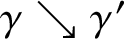
with the following property. Let C be an oriented curve on S, and let x be an essential crossing of C. Let
$C'$
be the oriented smoothing of C at x. Then
$f(C) \ge f(C')-R$
. Schematically, we have(1.2)See Definition 2.6 for ‘essential crossing’. Loosely, it is a crossing that cannot be removed by homotopy. See Definition 2.7 for ‘oriented smoothing’.
$R\ge 0$
with the following property. Let C be an oriented curve on S, and let x be an essential crossing of C. Let
$C'$
be the oriented smoothing of C at x. Then
$f(C) \ge f(C')-R$
. Schematically, we have(1.2)See Definition 2.6 for ‘essential crossing’. Loosely, it is a crossing that cannot be removed by homotopy. See Definition 2.7 for ‘oriented smoothing’. -
• Smoothing: We take
$R=0$
in the above definition of quasi-smoothing:(1.3) -
• Convex union: Let
$C_1$
and
$C_2$
be two oriented curves on S. Then(1.4)
$$ \begin{align} f(C_1 \cup C_2) \le f(C_1) + f(C_2). \end{align} $$
-
• Additive union: The inequality in convex union becomes an equality:
(1.5)
$$ \begin{align} f(C_1 \cup C_2) = f(C_1) + f(C_2). \end{align} $$


Table 1 Notation for the objects related to surfaces, curves and geodesic currents.

Many natural curve functionals satisfy the additive union property; for instance, length with respect to an arbitrary length metric on S satisfies it by definition. The square root of extremal length is an example of a curve functional satisfying convex union but not additive union (Subsection 4.8). The name ‘convex union’ comes from the fact that if we extend to weighted curves and additionally assume homogeneity (Definition 1.7), then for a fixed oriented multi-curve with varying weights, f is a convex as a function of the weights (Proposition 3.4).
There are many curve functionals satisfying the smoothing property, such as hyperbolic length, extremal length, intersection number with a fixed curve or length from a length metric on S. For an example of a natural curve functional that satisfies quasi-smoothing but not smoothing, we have the word length with respect to an arbitrary generating set of
 $\pi _1(S)$
(Example 4.10). The (quasi-)smoothing property is usually easy to check.
$\pi _1(S)$
(Example 4.10). The (quasi-)smoothing property is usually easy to check.
The smoothing property plays an important role in the study of translation lengths associated to Anosov representations, as we discuss in Subsection 4.7, following Martone and Zhang [Reference Martone and Zhang38] and Burger et al. [Reference Burger, Iozzi, Parreau and Pozzetti13]. These works use the smoothing property to reduce the study of length systoles to the case of simple closed curves. Although these papers point out the parallelism between the smoothing property of Anosov translation lengths and that of hyperbolic length ([Reference Burger, Iozzi, Parreau and Pozzetti13, Section 4] or negatively curved lengths [Reference Martone and Zhang38, Corollary 1.3], the results in our article reveal the much more universal nature of the smoothing property. Indeed, we show many other natural notions of lengths which are not associated to negatively curved structures satisfy the smoothing condition, such as lengths on Riemannian metrics with no curvature assumption, lengths coming from more general length space structures, extremal lengths or word lengths with respect to certain generating sets; see Section 4.
Definition 1.6. For C an oriented multi-curve,
 $nC$
is the oriented multi-curve that consists of n parallel copies of C (so with n times as many components or, in the context of weighted oriented multi-curves, with weights multiplied by n), and
$nC$
is the oriented multi-curve that consists of n parallel copies of C (so with n times as many components or, in the context of weighted oriented multi-curves, with weights multiplied by n), and
 $C^n$
is the oriented multi-curve with as many components as C, in which each component of C is covered by an n-fold cover. That is, if
$C^n$
is the oriented multi-curve with as many components as C, in which each component of C is covered by an n-fold cover. That is, if
 $g \in \pi _1(S,x)$
represents C,
$g \in \pi _1(S,x)$
represents C,
 $g^n$
represents
$g^n$
represents
 $C^n$
.
$C^n$
.
Definition 1.7. Let f be a curve functional and let
 $n>0$
be an integer. We define some properties f might satisfy:
$n>0$
be an integer. We define some properties f might satisfy:
-
• Homogeneity: For an arbitrary oriented multi-curve C,
(1.8)
$$ \begin{align} f(nC) = nf(C). \end{align} $$
-
• (Weak) stability: For an arbitrary oriented multi-curve C,
(1.9)
$$ \begin{align} f(C^n) = f(nC). \end{align} $$
-
• Strong stability: For arbitrary oriented multi-curves
$C,D$
,(1.10)
$$ \begin{align} f(D\cup C^n) = f(D\cup nC). \end{align} $$


Additive union implies homogeneity, and if f satisfies convex union,
 $f(nC) \le nf(C)$
. If f satisfies quasi-smoothing, then
$f(nC) \le nf(C)$
. If f satisfies quasi-smoothing, then
 $f(nC) -nR \le f(C^n)$
, since the self-crossings in
$f(nC) -nR \le f(C^n)$
, since the self-crossings in
 $C^n$
are essential crossings by definition (see Definition 2.6).
$C^n$
are essential crossings by definition (see Definition 2.6).
We furthermore note that curve functionals are not necessarily positive.
With this background, we can state our main theorems on extensions of curve functionals to the space
 $\mathcal {GC}^+(S)$
of oriented geodesic currents.
$\mathcal {GC}^+(S)$
of oriented geodesic currents.
Theorem A. Let f be a curve functional satisfying the quasi-smoothing, convex union, stability and homogeneity properties. Then there is a unique continuous homogeneous function
 $\bar {f} \colon \mathcal {GC}^+(S) \to \mathbb {R}_{\ge 0}$
that extends f.
$\bar {f} \colon \mathcal {GC}^+(S) \to \mathbb {R}_{\ge 0}$
that extends f.
In the case of unoriented curves, there are two possible smoothings of an essential crossing, not distinguished from each other. Then we have the following version of the theorem, deduced from Theorem A in Subsection 2.5.
Corollary 1.11. Let f be an unoriented curve functional satisfying quasi-smoothing for both possible smoothings of a crossing, in addition to the convex union, stability and homogeneity properties. Then there is a unique continuous homogeneous function
 $\bar {f} \colon \mathcal {GC}(S) \to \mathbb {R}$
that extends f.
$\bar {f} \colon \mathcal {GC}(S) \to \mathbb {R}$
that extends f.
Theorem A should be thought of as an analogue of the classical theorem that a convex function defined on the rational points in a finite-dimensional vector space automatically extends continuously to a convex function defined on the whole vector space (Proposition 3.1(iv)). As in the classical case, the functions on geodesic currents arising from this construction are restricted, as the next example shows. (This example is almost the only function we are aware of where our techniques do not suffice to prove continuity of the extension. See Subsection 4.1.)
Example 1.12. Consider the curve curves given by the square root of self-intersection number; that is,
 $f(C) := \sqrt {i(C,C)}$
. Since intersection number is a continuous two-variable function [Reference Bonahon10, Proposition 4.5], it follows that f extends continuously to geodesic currents. However, f does not satisfy convex union. For instance, take
$f(C) := \sqrt {i(C,C)}$
. Since intersection number is a continuous two-variable function [Reference Bonahon10, Proposition 4.5], it follows that f extends continuously to geodesic currents. However, f does not satisfy convex union. For instance, take
 $C_1$
and
$C_1$
and
 $C_2$
to be two simple closed curves intersecting once. For any multi-curve,
$C_2$
to be two simple closed curves intersecting once. For any multi-curve,
 $i(C,C)$
is twice the self-intersection number of C. Thus,
$i(C,C)$
is twice the self-intersection number of C. Thus,
 $f(C_1 \cup C_2)=\sqrt {2}$
, but
$f(C_1 \cup C_2)=\sqrt {2}$
, but
 $f(C_1)+ f(C_2) = 0$
, contradicting convex union. On the other hand, f clearly satisfies smoothing.
$f(C_1)+ f(C_2) = 0$
, contradicting convex union. On the other hand, f clearly satisfies smoothing.
On the other hand, the stability and homogeneous properties are necessary conditions for an extension to exist for elementary reasons, as the multi-curves
 $nC$
and
$nC$
and
 $C^n$
should represent the same currents (Example 4.10). However, a curve functional that satisfies quasi-smoothing and convex union can be modified to get a curve functional satisfying all the hypotheses of Theorem A.
$C^n$
should represent the same currents (Example 4.10). However, a curve functional that satisfies quasi-smoothing and convex union can be modified to get a curve functional satisfying all the hypotheses of Theorem A.
Theorem B. Let f be a curve functional satisfying quasi-smoothing and convex union. Then the stabilised curve functional
 $$ \begin{align*} \|f\|(C) := \lim_{n \to \infty} \frac{f(C^n)}{n} \end{align*} $$
satisfies quasi-smoothing, convex union, strong stability and homogeneity and thus extends to a continuous function on
 $\mathcal {GC}^+(S)$
.
$\mathcal {GC}^+(S)$
.
Theorem B is proved in Subsection 13, although the implication that weak stability implies strong stability is used in the proof of Theorem A.
If the convex union property of f is strengthened to additive union and the quasi-smoothing property is strengthened to smoothing, then in fact this extension to geodesic currents comes from intersection with a fixed current (as in the proofs of extension that used Bonahon’s principle). This will appear in a forthcoming paper. For this stronger result, the strict smoothing property is necessary, since intersection number cannot increase after smoothing an essential crossing.
2 Background on curves and currents
Throughout this article, S is a fixed oriented compact 2-manifold without boundary. (For a discussion of the more general surface case, see Remark 2.26.) If we fix an arbitrary (hyperbolic) metric on S, we will denote it by
 $\Sigma $
. The various types of curves and associated objects we consider are summarised in Table 1.
$\Sigma $
. The various types of curves and associated objects we consider are summarised in Table 1.
2.1 Curves
Definition 2.1 multi-curve
A concrete multi-curve
 $\gamma $
on a surface S is a smooth 1-manifold without boundary
$\gamma $
on a surface S is a smooth 1-manifold without boundary
 $X(\gamma )$
together with a map (also called
$X(\gamma )$
together with a map (also called
 $\gamma $
) from
$\gamma $
) from
 $X(\gamma )$
into S.
$X(\gamma )$
into S.
 $X(\gamma )$
is not necessarily connected. We say that
$X(\gamma )$
is not necessarily connected. We say that
 $\gamma $
is trivial if it is homotopic to a point. Two concrete multi-curves
$\gamma $
is trivial if it is homotopic to a point. Two concrete multi-curves
 $\gamma $
and
$\gamma $
and
 $\gamma '$
are equivalent if they are related by a sequence of the following moves:
$\gamma '$
are equivalent if they are related by a sequence of the following moves:
-
• homotopy within the space of all maps from
$X(\gamma )$
to S; -
• reparametrisation of the 1-manifold; and
-
• dropping trivial components.

The equivalence class of
 $\gamma $
is denoted by
$\gamma $
is denoted by
 $[\gamma ]$
, and we will call it a multi-curve. If
$[\gamma ]$
, and we will call it a multi-curve. If
 $X(\gamma )$
is connected, we will call
$X(\gamma )$
is connected, we will call
 $[\gamma ]$
a curve; a curve is equivalent to a conjugacy class in
$[\gamma ]$
a curve; a curve is equivalent to a conjugacy class in
 $\pi _1(S)$
. When we just want to refer to the equivalence class of a (multi-)curve, without distinguishing a representative, we will use capital letters such as C. A concrete multi-curve
$\pi _1(S)$
. When we just want to refer to the equivalence class of a (multi-)curve, without distinguishing a representative, we will use capital letters such as C. A concrete multi-curve
 $\gamma $
is simple if
$\gamma $
is simple if
 $\gamma $
is injective, and a multi-curve is simple if it has a concrete representative that is simple. We write
$\gamma $
is injective, and a multi-curve is simple if it has a concrete representative that is simple. We write
 $\mathcal {S}(S)$
for the space of simple multi-curves on S and
$\mathcal {S}(S)$
for the space of simple multi-curves on S and
 $\mathcal {C}(S)$
for the space of all multi-curves.
$\mathcal {C}(S)$
for the space of all multi-curves.
We also consider oriented multi-curves, which we will still denote by
 $\gamma $
, in which
$\gamma $
, in which
 $X(\gamma )$
is oriented. We add the further condition in the equivalence relation that the reparametrisations must be orientation-preserving. In this article, unless stated otherwise, we will be working with oriented multi-curves. The spaces of oriented simple and general multi-curves are denoted
$X(\gamma )$
is oriented. We add the further condition in the equivalence relation that the reparametrisations must be orientation-preserving. In this article, unless stated otherwise, we will be working with oriented multi-curves. The spaces of oriented simple and general multi-curves are denoted
 $\mathcal {S}^+(S)$
and
$\mathcal {S}^+(S)$
and
 $\mathcal {C}^+(S)$
, respectively.
$\mathcal {C}^+(S)$
, respectively.
Definition 2.2 weighted multi-curve
A weighted multi-curve
 $C=\bigcup _i a_i C_i$
is a multi-curve in which each connected component is given a nonnegative real coefficient
$C=\bigcup _i a_i C_i$
is a multi-curve in which each connected component is given a nonnegative real coefficient
 $a_i$
. If coefficients are not specified, they are
$a_i$
. If coefficients are not specified, they are
 $1$
. We add further moves to the equivalence relation:
$1$
. We add further moves to the equivalence relation:
-
• merging two parallel components and adding their weights and
-
• nullifying, deleting a component with weight
$0$
.

For instance,
 $C \cup C$
is equivalent to
$C \cup C$
is equivalent to
 $2C$
. The space of weighted multi-curves up to equivalence is denoted by appending an
$2C$
. The space of weighted multi-curves up to equivalence is denoted by appending an
 $\mathbb {R}$
in front of their nonweighted names, so
$\mathbb {R}$
in front of their nonweighted names, so
 $\mathbb {R}\mathcal {S}(S)$
is the space of weighted simple multi-curves and
$\mathbb {R}\mathcal {S}(S)$
is the space of weighted simple multi-curves and
 $\mathbb {R}\mathcal {C}(S)$
is the space of weighted general multi-curves. This is a slight abuse of notation since the weights are required to be nonnegative.
$\mathbb {R}\mathcal {C}(S)$
is the space of weighted general multi-curves. This is a slight abuse of notation since the weights are required to be nonnegative.
Remark 2.3. Since the weighted curve functionals we are considering are not necessarily positive, they may increase after dropping a component (see Definition 2.2).
2.2 Crossings
Loosely speaking, an essential crossing is a crossing of a multi-curve that cannot be homotoped away. We make this definition precise as follows. We cover cases where
 $\gamma $
does not have transverse crossings for convenience of some of the examples.
$\gamma $
does not have transverse crossings for convenience of some of the examples.
Definition 2.4 linked points on a circle
We say that two sets of two points
 $\{a,b\}$
and
$\{a,b\}$
and
 $\{c,d\}$
in
$\{c,d\}$
in
 $S^1$
are linked if the four points are distinct and both connected components of
$S^1$
are linked if the four points are distinct and both connected components of
 $S^1- \{ a,b \}$
have an element of
$S^1- \{ a,b \}$
have an element of
 $\{c,d\}$
.
$\{c,d\}$
.
Definition 2.5 lift of a concrete curve
Given a concrete multi-curve
 $\gamma $
on S and a choice
$\gamma $
on S and a choice
 $p \in X(\gamma )$
, set
$p \in X(\gamma )$
, set
 $x=\gamma (p) \in S$
. Pick a lift
$x=\gamma (p) \in S$
. Pick a lift
 $\widetilde {x} \in \widetilde {S}$
of x. The unique lifting property gives a unique lift
$\widetilde {x} \in \widetilde {S}$
of x. The unique lifting property gives a unique lift
 $\widetilde {\gamma _p}: \widetilde {X}(\gamma ;p) \to \widetilde {S}$
of
$\widetilde {\gamma _p}: \widetilde {X}(\gamma ;p) \to \widetilde {S}$
of
 $\gamma $
with
$\gamma $
with
 $\widetilde {\gamma _p}(\widetilde {p}) = \widetilde {x}$
, where
$\widetilde {\gamma _p}(\widetilde {p}) = \widetilde {x}$
, where
 $X(\gamma ;p)$
is the component of
$X(\gamma ;p)$
is the component of
 $X(\gamma )$
containing p and
$X(\gamma )$
containing p and
 $\widetilde {X}(\gamma ;p)$
is its universal cover with basepoint
$\widetilde {X}(\gamma ;p)$
is its universal cover with basepoint
 $\widetilde {p}$
.
$\widetilde {p}$
.
Definition 2.6 essential crossing
Let
 $\gamma $
be a concrete multi-curve on S, and suppose we have points
$\gamma $
be a concrete multi-curve on S, and suppose we have points
 $p,q \in X(\gamma )$
so that
$p,q \in X(\gamma )$
so that
 $x := \gamma (p) = \gamma (q) \in S$
. Pick a lift
$x := \gamma (p) = \gamma (q) \in S$
. Pick a lift
 $\widetilde {x} \in \widetilde {S}$
of x, and let
$\widetilde {x} \in \widetilde {S}$
of x, and let
 $\widetilde {\gamma _p}$
and
$\widetilde {\gamma _p}$
and
 $\widetilde {\gamma _q}$
be the corresponding lifts of components of
$\widetilde {\gamma _q}$
be the corresponding lifts of components of
 $\gamma $
following Definition 2.5. Then the pair
$\gamma $
following Definition 2.5. Then the pair
 $(p,q)$
form an essential crossing if the following two conditions hold:
$(p,q)$
form an essential crossing if the following two conditions hold:
-
(1) both components of
$X(\gamma )$
containing p and q are not null-homotopic, so that
$\widetilde {\gamma _p}$
and
$\widetilde {\gamma _q}$
are quasi-geodesic components of
$\widetilde {\gamma }$
and -
(2) either
-
(a) the endpoints
$\{a,b\}$
of
$\widetilde {\gamma _p}$
and the endpoints
$\{c,d\}$
of
$\widetilde {\gamma _q}$
are linked in
$S^1_\infty $
or -
(b) p and q lie on the same component of
$X(\gamma )$
,
$[\gamma ] = [\delta ^n]$
for some
$n> 1$
and some primitive
$\delta \in \pi _1(S,x)$
, the loop from p to q in
$X(\gamma )$
maps to
$[\delta ^m]$
for some
$0 < m < n$
and so the loop from q to p maps to
$[\delta ^{n-m}]$
.
-


In case (2)b, the endpoints of
 $\widetilde {\gamma _p}$
and
$\widetilde {\gamma _p}$
and
 $\widetilde {\gamma _q}$
are the same.
$\widetilde {\gamma _q}$
are the same.
This definition might be somewhat looser than expected. For instance, in the chain of three crossings

the circled middle crossing is essential iff the other two are, since ‘linking at infinity’ does not see the direction of crossing. This does not matter for our purposes.
Definition 2.7 smoothings
Let
 $(p,q) \in X(\gamma )$
be an essential crossing of
$(p,q) \in X(\gamma )$
be an essential crossing of
 $\gamma $
on S. To make a smoothing
$\gamma $
on S. To make a smoothing
 $\gamma '$
of
$\gamma '$
of
 $(p,q)$
, cut
$(p,q)$
, cut
 $X(\gamma )$
at p and q and reglue the resulting four endpoints in one of the two other possible ways, getting a new
$X(\gamma )$
at p and q and reglue the resulting four endpoints in one of the two other possible ways, getting a new
 $1$
-manifold
$1$
-manifold
 $X(\gamma ')$
. The map
$X(\gamma ')$
. The map
 $\gamma '$
agrees with
$\gamma '$
agrees with
 $\gamma $
; this is well-defined since
$\gamma $
; this is well-defined since
 $\gamma (p) = \gamma (q)$
. In pictures we will homotop
$\gamma (p) = \gamma (q)$
. In pictures we will homotop
 $\gamma '$
slightly to round out the resulting corners. If
$\gamma '$
slightly to round out the resulting corners. If
 $\gamma $
is oriented, then the oriented smoothing is the smoothing that respects the orientation on
$\gamma $
is oriented, then the oriented smoothing is the smoothing that respects the orientation on
 $X(\gamma )$
:
$X(\gamma )$
:

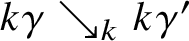
If we obtain a concrete curve
 $\gamma '$
from
$\gamma '$
from
 $\gamma $
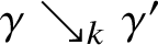
by a sequence of k smoothings of essential crossings, we will write
$\gamma $
by a sequence of k smoothings of essential crossings, we will write
 $\gamma \mathrel {\searrow }_k \gamma '$
. (We check whether the crossings are essential at each stage of this process; this is more restrictive than checking at the beginning.)
$\gamma \mathrel {\searrow }_k \gamma '$
. (We check whether the crossings are essential at each stage of this process; this is more restrictive than checking at the beginning.)
Lemma 2.8. Essential crossings are unavoidable in a homotopy class, in the sense that if
 $\gamma $
and
$\gamma $
and
 $\gamma '$
are homotopic concrete multi-curves and
$\gamma '$
are homotopic concrete multi-curves and
 $(p,q) \in X(\gamma )$
is an essential crossing of
$(p,q) \in X(\gamma )$
is an essential crossing of
 $\gamma $
, then there is an essential crossing
$\gamma $
, then there is an essential crossing
 $(p',q') \in X(\gamma ')$
so that the smoothings of
$(p',q') \in X(\gamma ')$
so that the smoothings of
 $(p,q)$
and
$(p,q)$
and
 $(p',q')$
are homotopic.
$(p',q')$
are homotopic.
Proof. For both types of essential crossings, there is a representative
 $\gamma '$
with minimal crossing number for which the result is clear:
$\gamma '$
with minimal crossing number for which the result is clear:
-
(a) For crossings of the first type, take the geodesic representative on S, perturbed slightly to make it transverse.
-
(b) For crossings of the second type
$[\gamma ] = [\delta ^n]$
, take the geodesic representative and perturb it slightly in a standard way in a neighbourhood of
$\delta $
.

In general, take the given representative
 $\gamma $
and perturb it slightly to make it transverse (without introducing new types of crossings). If
$\gamma $
and perturb it slightly to make it transverse (without introducing new types of crossings). If
 $\gamma $
is connected, then by a result of Hass and Scott [Reference Hass and Scott30, Theorems 1.8 and 2.1] (see also de Graaf and Schrijver [Reference de Graaf and Schrijver18]),
$\gamma $
is connected, then by a result of Hass and Scott [Reference Hass and Scott30, Theorems 1.8 and 2.1] (see also de Graaf and Schrijver [Reference de Graaf and Schrijver18]),
 $\gamma $
can be turned into any desired minimal form
$\gamma $
can be turned into any desired minimal form
 $\gamma '$
using only Reidemeister I, II and III moves, with the Reidemeister I and II moves being used only in the forward (simplifying) direction. Since we know that
$\gamma '$
using only Reidemeister I, II and III moves, with the Reidemeister I and II moves being used only in the forward (simplifying) direction. Since we know that
 $\gamma '$
has a crossing of the desired type, we can trace the crossings backwards through these moves: a Reidemeister III move does not change the homotopy types of curves achievable by a single smoothing, and we can ignore the additional crossings created by backwards Reidemeister I and II moves.
$\gamma '$
has a crossing of the desired type, we can trace the crossings backwards through these moves: a Reidemeister III move does not change the homotopy types of curves achievable by a single smoothing, and we can ignore the additional crossings created by backwards Reidemeister I and II moves.
For multi-curves, the papers above also prove that any diagram can be connected to a minimal diagram by a series of forward Reidemeister moves and that the only obstruction to connecting two minimal diagrams for a multi-curve is swapping the location of two components
 $\gamma _1, \gamma _2$
that are homotopically powers of the same primitive curve
$\gamma _1, \gamma _2$
that are homotopically powers of the same primitive curve
 $\delta $
[Reference Hass and Scott30, pp. 31–32]. But any of these minimal representatives in a neighbourhood of
$\delta $
[Reference Hass and Scott30, pp. 31–32]. But any of these minimal representatives in a neighbourhood of
 $\delta $
contain all essential crossings between
$\delta $
contain all essential crossings between
 $\gamma _1$
and
$\gamma _1$
and
 $\gamma _2$
(necessarily related to an essential self-crossing of
$\gamma _2$
(necessarily related to an essential self-crossing of
 $\delta $
).
$\delta $
).
Remark 2.9. We can also see directly that essential crossings of the first type exist by considering the lift to the universal cover. Lemma 2.8 is false on nonorientable surfaces (consider the double cover of the core curve of a Möbius strip).
We have similar notions for weighted curves.
Definition 2.10. Let
 $C \in \mathbb {R}\mathcal {C}^+(S)$
be a weighted oriented curve, and let
$C \in \mathbb {R}\mathcal {C}^+(S)$
be a weighted oriented curve, and let
 $\gamma $
be a concrete representative of the underlying unweighted curve. Let
$\gamma $
be a concrete representative of the underlying unweighted curve. Let
 $(p,q) \in X(\gamma )$
be an essential crossing of
$(p,q) \in X(\gamma )$
be an essential crossing of
 $\gamma $
on S, and let
$\gamma $
on S, and let
 $\gamma '$
be the smoothing as defined above. If the corresponding components of C have equal weight
$\gamma '$
be the smoothing as defined above. If the corresponding components of C have equal weight
 $w> 0$
, then we can make a weighted curve
$w> 0$
, then we can make a weighted curve
 $C'$
by giving every component in
$C'$
by giving every component in
 $[\gamma ']$
not involved in the smoothing the same weight it had in C and giving the one or two new components weight w. In this case we say that
$[\gamma ']$
not involved in the smoothing the same weight it had in C and giving the one or two new components weight w. In this case we say that
 $C'$
is obtained from C by a smoothing of weight w and write
$C'$
is obtained from C by a smoothing of weight w and write
 $C \mathrel {\searrow }_w C'$
.
$C \mathrel {\searrow }_w C'$
.
Using this, we define conditions on a weighted curve functional, extending Definition 1.1.
-
• Weighted quasi-smoothing: There is a constant
$R>0$
so that
$C \mathrel {\searrow }_w C'$
are weighted curves related by a smoothing of weight w,
$$ \begin{align*} f(C) \ge f(C')-wR. \end{align*} $$
-
• Weighted smoothing: Take
$R=0$
in the definition of weighted quasi-smoothing.


See Proposition 3.6 for justification for these definitions.
2.3 Space of geodesics
Definition 2.11 Boundary at infinity
Endow S with a complete hyperbolic metric g; we denote the pair
 $(S,g)$
by
$(S,g)$
by
 $\Sigma $
. Then we can consider the metric universal covering
$\Sigma $
. Then we can consider the metric universal covering
 $p \colon \widetilde {\Sigma } \to \Sigma $
, with
$p \colon \widetilde {\Sigma } \to \Sigma $
, with
 $\widetilde {\Sigma }$
isometric to the hyperbolic plane. Two quasi-geodesic rays
$\widetilde {\Sigma }$
isometric to the hyperbolic plane. Two quasi-geodesic rays
 $c,c' \colon [0,\infty ) \to \widetilde {\Sigma }$
are said to be asymptotic if there exists a constant K for which
$c,c' \colon [0,\infty ) \to \widetilde {\Sigma }$
are said to be asymptotic if there exists a constant K for which
 $d(c(t),c'(t)) \leq K$
for all
$d(c(t),c'(t)) \leq K$
for all
 $t \geq 0$
. We define
$t \geq 0$
. We define
 $\partial _{\infty } \Sigma $
, the boundary at infinity of S, to be the set of equivalence classes of asymptotic quasi-geodesic rays. This boundary at infinity is independent of the hyperbolic structure on S up to canonical homeomorphism.
$\partial _{\infty } \Sigma $
, the boundary at infinity of S, to be the set of equivalence classes of asymptotic quasi-geodesic rays. This boundary at infinity is independent of the hyperbolic structure on S up to canonical homeomorphism.
Definition 2.12 Space of oriented geodesics
Let
 $G^{+}(\Sigma )$
denote the space of oriented geodesics in
$G^{+}(\Sigma )$
denote the space of oriented geodesics in
 $\widetilde {\Sigma }$
; that is,
$\widetilde {\Sigma }$
; that is,
 $$ \begin{align*} G^+(\Sigma) :=\partial_\infty \Sigma \times\partial_\infty\Sigma - \Delta. \end{align*} $$
Since this is independent of the hyperbolic structure, we will also write
 $G^+(S)$
.
$G^+(S)$
.
2.4 Geodesic currents
Definition 2.13 Geodesic current definition 1
We define
 $\mathcal {GC}^+(S)$
, the space of oriented geodesic currents on S, to be the space of
$\mathcal {GC}^+(S)$
, the space of oriented geodesic currents on S, to be the space of
 $\pi _1(S)$
-invariant (positive) Radon measures on
$\pi _1(S)$
-invariant (positive) Radon measures on
 $G^{+}(S)$
.
$G^{+}(S)$
.
Since the action of
 $\pi _1(S)$
on
$\pi _1(S)$
on
 $G^+(S)$
is not discrete, this definition is hard to visualise. We give alternate definitions that play a key role in our proofs. For a hyperbolic surface
$G^+(S)$
is not discrete, this definition is hard to visualise. We give alternate definitions that play a key role in our proofs. For a hyperbolic surface
 $\Sigma $
, let
$\Sigma $
, let
 $UT\Sigma $
be the unit tangent bundle and let
$UT\Sigma $
be the unit tangent bundle and let
 $\phi _t$
be the geodesic flow on it.
$\phi _t$
be the geodesic flow on it.
Definition 2.14 Geodesic current definition 2
We can also define oriented geodesic currents to be the space of (positive) finite Radon measures
 $\mu $
on
$\mu $
on
 $UT \Sigma $
which are invariant under the geodesic flow, in the sense that
$UT \Sigma $
which are invariant under the geodesic flow, in the sense that
 $(\phi _t)_*(\mu ) = \mu $
for all
$(\phi _t)_*(\mu ) = \mu $
for all
 $t\in \mathbb {R}$
.
$t\in \mathbb {R}$
.
We can also look at induced measures on cross sections.
Definition 2.15 Geodesic current definition 3
A geodesic current is a transverse invariant measure: a family of measures
 $\{\mu _{\tau }\}_{\tau }$
, where
$\{\mu _{\tau }\}_{\tau }$
, where
 $\tau \subset UT \Sigma $
is a submanifold-with-boundary of the unit tangent bundle of real codimension 1 transverse to the geodesic foliation
$\tau \subset UT \Sigma $
is a submanifold-with-boundary of the unit tangent bundle of real codimension 1 transverse to the geodesic foliation
 $\mathcal {F}$
, with the following invariance property: if
$\mathcal {F}$
, with the following invariance property: if
 $x_1 \in \tau _1, x_2 \in \tau _2$
are two points on transversal submanifolds on the same leaf of
$x_1 \in \tau _1, x_2 \in \tau _2$
are two points on transversal submanifolds on the same leaf of
 $\mathcal {F}$
and
$\mathcal {F}$
and
 $\phi \colon U_1 \to U_2$
a holonomy diffeomorphism between neighbourhoods of
$\phi \colon U_1 \to U_2$
a holonomy diffeomorphism between neighbourhoods of
 $x_1$
and
$x_1$
and
 $x_2$
respectively, then
$x_2$
respectively, then
 $\phi _{*}\mu _{\tau _1}=\mu _{\tau _2}$
.
$\phi _{*}\mu _{\tau _1}=\mu _{\tau _2}$
.
The equivalence of the three definitions was known to Bonahon [Reference Bonahon10, Chapter 4]. Details can be found in [Reference Aramayona and Leininger1, Section 3.4]. Briefly, given a measure
 $\mu $
on
$\mu $
on
 $UT\Sigma $
as in Definition 2.14 and a cross section
$UT\Sigma $
as in Definition 2.14 and a cross section
 $\tau $
, there is an induced flux
$\tau $
, there is an induced flux
 $\mu _\tau $
on
$\mu _\tau $
on
 $\tau $
, as explained in Definition 7.15; this gives a geodesic current in the sense of Definition 2.15. Lifting to the universal cover then gives a geodesic current in the sense of Definition 2.13. We can also relate Definitions 2.13 and 2.14 directly by connecting both to measures on
$\tau $
, as explained in Definition 7.15; this gives a geodesic current in the sense of Definition 2.15. Lifting to the universal cover then gives a geodesic current in the sense of Definition 2.13. We can also relate Definitions 2.13 and 2.14 directly by connecting both to measures on
 $UT\mathbb {H}^2$
that are invariant under both
$UT\mathbb {H}^2$
that are invariant under both
 $\pi _1(\Sigma )$
and the geodesic flow, as described by Benoist and Oh [Reference Benoist and Oh7, Proposition 8.1].
$\pi _1(\Sigma )$
and the geodesic flow, as described by Benoist and Oh [Reference Benoist and Oh7, Proposition 8.1].
Because Definitions 2.13 and 2.15 are invariant under the mapping class group, we will also write
 $G^+(S)$
and
$G^+(S)$
and
 $\mathcal {GC}^+(S)$
in the sequel. We will also write
$\mathcal {GC}^+(S)$
in the sequel. We will also write
 $\pi _1(S)$
. On the other hand, we will emphasise the dependence of
$\pi _1(S)$
. On the other hand, we will emphasise the dependence of
 $UT\Sigma $
on the hyperbolic structure.
$UT\Sigma $
on the hyperbolic structure.
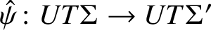
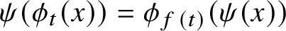
Remark 2.16. For
 $\Sigma ,\Sigma '$
hyperbolic surfaces, any homeomorphism
$\Sigma ,\Sigma '$
hyperbolic surfaces, any homeomorphism
 $\psi \colon \Sigma \to \Sigma '$
, there is a homeomorphism
$\psi \colon \Sigma \to \Sigma '$
, there is a homeomorphism
 $\hat \psi \colon UT\Sigma \to UT\Sigma '$
that is an orbit equivalence, and it is tempting to use this to define an induced map between geodesic currents in the sense of Definition 2.14. But this does not quite work:
$\hat \psi \colon UT\Sigma \to UT\Sigma '$
that is an orbit equivalence, and it is tempting to use this to define an induced map between geodesic currents in the sense of Definition 2.14. But this does not quite work:
 $\hat \psi _*$
does not take geodesic currents to geodesic currents. Orbit equivalence means that
$\hat \psi _*$
does not take geodesic currents to geodesic currents. Orbit equivalence means that
 $\psi (\phi _t(x)) = \phi _{f(t)}(\psi (x))$
for some monotonic function
$\psi (\phi _t(x)) = \phi _{f(t)}(\psi (x))$
for some monotonic function
 $f \colon \mathbb {R} \to \mathbb {R}$
, but this is not enough to guarantee that
$f \colon \mathbb {R} \to \mathbb {R}$
, but this is not enough to guarantee that
 $(\phi _t)_*(\hat \psi _*\mu ) = \hat \psi _*\mu $
, and, indeed, this is usually false. See Wilkinson [Reference Wilkinson61, Theorem 3.6].
$(\phi _t)_*(\hat \psi _*\mu ) = \hat \psi _*\mu $
, and, indeed, this is usually false. See Wilkinson [Reference Wilkinson61, Theorem 3.6].
2.5 Oriented vs unoriented currents
We will be mostly working in the setting of oriented geodesic currents, but most of our natural examples (like measured laminations) use unoriented currents.
Definition 2.17 Unoriented geodesic currents
To define the subspace
 $\mathcal {GC}(S) \subset \mathcal {GC}^{+}(S)$
of unoriented geodesics currents, let
$\mathcal {GC}(S) \subset \mathcal {GC}^{+}(S)$
of unoriented geodesics currents, let
 $\sigma : G^{+}(S) \to G^{+}(S)$
be the flip map that switches the two factors in the definition of
$\sigma : G^{+}(S) \to G^{+}(S)$
be the flip map that switches the two factors in the definition of
 $G^+(S)$
, reversing the orientation of the geodesic. This induces a map
$G^+(S)$
, reversing the orientation of the geodesic. This induces a map
 $\sigma _* \colon \mathcal {GC}^{+}(S) \to \mathcal {GC}^{+}(S)$
. Set
$\sigma _* \colon \mathcal {GC}^{+}(S) \to \mathcal {GC}^{+}(S)$
. Set
 $$ \begin{align*} \mathcal{GC}(\Sigma) := \{ \mu \in \mathcal{GC}^{+}(\Sigma) \mid \sigma_*(\mu)=\mu \}. \end{align*} $$
There is a map
 $\Pi \colon \mathcal {GC}^{+}(S) \to \mathcal {GC}^{+}(S)$
given by
$\Pi \colon \mathcal {GC}^{+}(S) \to \mathcal {GC}^{+}(S)$
given by
 $\Pi (\mu ):= \frac {1}{2}(\mu + \sigma _*(\mu ))$
with image the subset of unoriented currents.
$\Pi (\mu ):= \frac {1}{2}(\mu + \sigma _*(\mu ))$
with image the subset of unoriented currents.
In the proof of the main result, we shall work with oriented currents
 $\mathcal {GC}^+(S)$
; oriented currents are more general and just as easy to work with for our proof.
$\mathcal {GC}^+(S)$
; oriented currents are more general and just as easy to work with for our proof.
The maps
 $\sigma $
and
$\sigma $
and
 $\Pi $
have obvious analogues for curves.
$\Pi $
have obvious analogues for curves.
Proof of Corollary 1.11, assuming Theorem A. For a curve functional as in the statement, let
 $g \colon \mathbb {R} \mathcal {C}^+(S) \to \mathbb {R}$
be
$g \colon \mathbb {R} \mathcal {C}^+(S) \to \mathbb {R}$
be
 $f \circ \Pi $
. Then g satisfies quasi-smoothing, with the same constant as f, and thus by Theorem A extends uniquely to a continuous function
$f \circ \Pi $
. Then g satisfies quasi-smoothing, with the same constant as f, and thus by Theorem A extends uniquely to a continuous function
 $\bar g \colon \mathcal {GC}^+(S) \to \mathbb {R}$
. The desired extension
$\bar g \colon \mathcal {GC}^+(S) \to \mathbb {R}$
. The desired extension
 $\bar f$
is the restriction of
$\bar f$
is the restriction of
 $\bar g$
to the subspace of unoriented currents.
$\bar g$
to the subspace of unoriented currents.
2.6 Curves as currents
For an oriented multi-curve C on a hyperbolic surface
 $\Sigma $
, we can construct a geodesic current as follows.
$\Sigma $
, we can construct a geodesic current as follows.
For Definition 2.13, consider all lifts of all nontrivial components of C to
 $\widetilde {\Sigma }$
. Each lift gives a quasi-geodesic in
$\widetilde {\Sigma }$
. Each lift gives a quasi-geodesic in
 $\widetilde {\Sigma }$
and thus a unique fellow-travelling geodesic in
$\widetilde {\Sigma }$
and thus a unique fellow-travelling geodesic in
 $G^+(S)$
; we thus get an infinite countable subset of
$G^+(S)$
; we thus get an infinite countable subset of
 $G^+(S)$
, which is easily seen to be discrete and
$G^+(S)$
, which is easily seen to be discrete and
 $\pi _1(S)$
-invariant. Define the geodesic current to be the
$\pi _1(S)$
-invariant. Define the geodesic current to be the
 $\delta $
-function of this subset.
$\delta $
-function of this subset.
For Definition 2.14, take the geodesic representative
 $\gamma $
of C and consider the canonical lift
$\gamma $
of C and consider the canonical lift
 $\widetilde {\gamma }$
of
$\widetilde {\gamma }$
of
 $\gamma $
to
$\gamma $
to
 $UT\Sigma $
; this is an orbit of
$UT\Sigma $
; this is an orbit of
 $\phi _t$
. Let
$\phi _t$
. Let
 $\mu _C$
be the length-normalised
$\mu _C$
be the length-normalised
 $\delta $
-function on this orbit. That is, for an open set U we set
$\delta $
-function on this orbit. That is, for an open set U we set
 $\mu _C(U)$
to be the total length of
$\mu _C(U)$
to be the total length of
 $\widetilde {\gamma } \cap U$
with respect to the natural Riemannian metric on
$\widetilde {\gamma } \cap U$
with respect to the natural Riemannian metric on
 $UT\Sigma $
.
$UT\Sigma $
.
For Definition 2.15 on a cross section
 $\tau $
, again take
$\tau $
, again take
 $\widetilde {\gamma } \subset UT\Sigma $
, and let
$\widetilde {\gamma } \subset UT\Sigma $
, and let
 $\mu _\tau $
be the
$\mu _\tau $
be the
 $\delta $
-function on the discrete set of points
$\delta $
-function on the discrete set of points
 $\widetilde {\gamma } \cap \tau $
. (This is compatible with the length normalisation in the previous paragraph.)
$\widetilde {\gamma } \cap \tau $
. (This is compatible with the length normalisation in the previous paragraph.)
From any of these points of view the inclusion naturally extends to weighted multi-curves.
Weighted closed (multi-)curves are dense in the space of geodesic currents [Reference Bonahon10, Proposition 4.4].
Geometric intersection number extends continuously to geodesic currents, as shown by Bonahon [Reference Bonahon10, Proposition 4.5]. The space of measured laminations (defined by Harer and Penner [Reference Penner and Harer49, Section 1.7]) can be characterised, as in Bonahon [Reference Bonahon8, Proposition 17], as a subset of (unoriented) geodesic currents:
 $$ \begin{align*} \mathcal{ML}(S) := \{ \alpha \in \mathcal{GC}(S) \mid \sigma(\alpha)=\alpha, i(\alpha,\alpha)=0 \}. \end{align*} $$
The following square of inclusions is useful to keep in mind:

Here the horizontal inclusions have dense image: Douady and Hubbard showed that weighted simple multi-curves are dense in
 $\mathcal {ML}$
[Reference Douady and Hubbard19, Theorem]. Soon after, Masur showed that weighted simple curves are also dense [Reference Masur39, Theorem 1].
$\mathcal {ML}$
[Reference Douady and Hubbard19, Theorem]. Soon after, Masur showed that weighted simple curves are also dense [Reference Masur39, Theorem 1].
2.7 Topology on currents and measures
Let
 $\mathcal {M}(X)$
denote the space of positive Borel measures on a topological space X.
$\mathcal {M}(X)$
denote the space of positive Borel measures on a topological space X.
 $\mathcal {M}_1(X)$
will denote the space of Borel probability measures on X. The topology on
$\mathcal {M}_1(X)$
will denote the space of Borel probability measures on X. The topology on
 $\mathcal {M}(X)$
is the weak
$\mathcal {M}(X)$
is the weak
 $^*$
topology; that is, the smallest topology so that, for all continuous, compactly supported functions f on
$^*$
topology; that is, the smallest topology so that, for all continuous, compactly supported functions f on
 $G^+(S)$
, the functional
$G^+(S)$
, the functional
 $$ \begin{align*} \mu \mapsto \int_{G^+(S)} fd\mu \end{align*} $$
is continuous.
The topology on
 $\mathcal {GC}^+(S)$
(in Definition 2.13) is the weak
$\mathcal {GC}^+(S)$
(in Definition 2.13) is the weak
 $^*$
topology as a subspace of measures on
$^*$
topology as a subspace of measures on
 $G^+(S)$
, We could also look at the weak
$G^+(S)$
, We could also look at the weak
 $^*$
topology on currents as a subspace of measures on
$^*$
topology on currents as a subspace of measures on
 $UT\Sigma $
(Definition 2.14); these two points of view give the same topology [Reference Benoist and Oh7, Proposition 8.1]. On the other hand, if we take
$UT\Sigma $
(Definition 2.14); these two points of view give the same topology [Reference Benoist and Oh7, Proposition 8.1]. On the other hand, if we take
 $\tau $
to be a closed cross section (including the boundary), the map
$\tau $
to be a closed cross section (including the boundary), the map
 $\mu \mapsto \mu _\tau $
relating Definitions 2.14 and 2.15 is not usually continuous with respect to the weak
$\mu \mapsto \mu _\tau $
relating Definitions 2.14 and 2.15 is not usually continuous with respect to the weak
 $^*$
topologies, so it is delicate to use the weak
$^*$
topologies, so it is delicate to use the weak
 $^*$
topology on
$^*$
topology on
 $\mathcal {M}(\tau )$
; see Lemma 10.4 and Remark 10.6.
$\mathcal {M}(\tau )$
; see Lemma 10.4 and Remark 10.6.
There are in fact two topologies on spaces of measures that are sometimes called the weak
 $^*$
topology; the one above is also called the wide topology [Reference Minlos41, interalia]. There is also the narrow topology on measures
$^*$
topology; the one above is also called the wide topology [Reference Minlos41, interalia]. There is also the narrow topology on measures
 $\mathcal {M}(X)$
on a space X, defined as the smallest topology so that, for all continuous bounded f on X, the functional
$\mathcal {M}(X)$
on a space X, defined as the smallest topology so that, for all continuous bounded f on X, the functional
 $\mu \mapsto \int _{X} fd\mu $
is continuous. (That is, replace compactly supported with bounded in the functions considered.)
$\mu \mapsto \int _{X} fd\mu $
is continuous. (That is, replace compactly supported with bounded in the functions considered.)
Remark 2.18. Some authors call the weak
 $^*$
topology the vague topology and use the term weak topology for the narrow one (for example, Bauer’s textbook [Reference Bauer and Burckel6]). However, this conflicts with the notion of weak topology used for Banach spaces, and we prefer the wide/narrow usage.
$^*$
topology the vague topology and use the term weak topology for the narrow one (for example, Bauer’s textbook [Reference Bauer and Burckel6]). However, this conflicts with the notion of weak topology used for Banach spaces, and we prefer the wide/narrow usage.
In general, the weak
 $^*$
or wide topology is weaker than the narrow topology, but in some particular cases they are equivalent.
$^*$
or wide topology is weaker than the narrow topology, but in some particular cases they are equivalent.
A topological space X is called Polish if its topology has a countable base and can be defined by a complete metric.
Theorem 2.19 [Reference Bauer and Burckel6, Theorem 31.5]
Let X be a locally compact topological space. Then X is Polish if and only if
 $\mathcal {M}(X)$
is Polish with respect to the weak
$\mathcal {M}(X)$
is Polish with respect to the weak
 $^*$
-topology.
$^*$
-topology.
Thus,
 $\mathcal {GC}^+(S)$
is second countable completely metrisable and second countable and so in particular sequential continuity is the same as continuity. Although we will be dealing with Radon measures, for Polish spaces it is equivalent to consider the a priori more general class of Borel measures.
$\mathcal {GC}^+(S)$
is second countable completely metrisable and second countable and so in particular sequential continuity is the same as continuity. Although we will be dealing with Radon measures, for Polish spaces it is equivalent to consider the a priori more general class of Borel measures.
Theorem 2.20 [Reference Bauer and Burckel6, Theorem 26.3]
On a Polish space, a locally finite Borel measure is a
 $\sigma $
-finite Radon measure.
$\sigma $
-finite Radon measure.
The narrow and wide topology agree in certain sequences on locally compact spaces.
Theorem 2.21 [Reference Bauer and Burckel6, Theorem 30.8]
Let X be a locally compact topological space and
 $\mu _n$
a sequence of Radon measures of uniformly bounded mass converging to a Radon measure
$\mu _n$
a sequence of Radon measures of uniformly bounded mass converging to a Radon measure
 $\mu $
in the wide topology. Then
$\mu $
in the wide topology. Then
 $\mu _n$
converges to
$\mu _n$
converges to
 $\mu $
in the narrow topology if and only if
$\mu $
in the narrow topology if and only if
 $\lim _n \mu _n(X) \to \mu (X)$
.
$\lim _n \mu _n(X) \to \mu (X)$
.
Proposition 2.22 [Reference Bauer and Burckel6, Corollary 30.9]
Let X be a locally compact topological space and
 $\mu $
,
$\mu $
,
 $\mu _n$
Borel probability measures. Then
$\mu _n$
Borel probability measures. Then
 $\mu _n \to \mu $
in the wide topology if and only if
$\mu _n \to \mu $
in the wide topology if and only if
 $\mu _n \to \mu $
in the narrow topology.
$\mu _n \to \mu $
in the narrow topology.
In particular, when X is Polish, the two topologies agree for the space
 $\mathcal {M}_1(X)$
of Borel probability measures.
$\mathcal {M}_1(X)$
of Borel probability measures.
Proposition 2.23. If X is a locally compact Polish space, the weak
 $^*$
and narrow topologies agree on
$^*$
and narrow topologies agree on
 $\mathcal {M}_1(X)$
.
$\mathcal {M}_1(X)$
.
Convention 2.24. For any topological space X, we will always use the weak
 $^*$
topology on
$^*$
topology on
 $\mathcal {M}(X)$
. We will also work with the dense subspace
$\mathcal {M}(X)$
. We will also work with the dense subspace
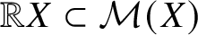 $\mathbb {R} X \subset \mathcal {M}(X)$
of finitely supported measures on X (also called weighted linear combinations of X), with its inherited subspace topology. (The weights are positive, but we usually omit that from the notation.)
$\mathbb {R} X \subset \mathcal {M}(X)$
of finitely supported measures on X (also called weighted linear combinations of X), with its inherited subspace topology. (The weights are positive, but we usually omit that from the notation.)
Remark 2.25. If we limit to sums with at most k terms in the linear combination (or points in the support of the measure), we get a further subspace temporarily denoted
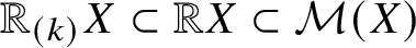 $\mathbb {R}_{(k)}X \subset \mathbb {R} X \subset \mathcal {M}(X)$
. We can view
$\mathbb {R}_{(k)}X \subset \mathbb {R} X \subset \mathcal {M}(X)$
. We can view
 $\mathbb {R}_{(k)} X$
as a quotient of
$\mathbb {R}_{(k)} X$
as a quotient of
 $(\mathbb {R}_{\ge 0} \times X)^k$
, quotienting by the action of the symmetric group and other evident equivalences; as such, it inherits an obvious topology, which agrees with the subspace topology.
$(\mathbb {R}_{\ge 0} \times X)^k$
, quotienting by the action of the symmetric group and other evident equivalences; as such, it inherits an obvious topology, which agrees with the subspace topology.
Remark 2.26. Geodesic currents can also be defined more generally for finite type hyperbolic surfaces. Depending on if we consider ends as cusps or funnels, we get two different spaces, which we will call
 $\mathcal {GC}_{\mathrm {cusp}}(S)$
and
$\mathcal {GC}_{\mathrm {cusp}}(S)$
and
 $\mathcal {GC}_{\mathrm {open}}(S)$
, respectively. In the first case, we define the space of geodesic currents analogously to Definition 2.13 for closed surfaces; that is, as invariant measures supported on the space of geodesics of the universal cover, noting that now the space of geodesics contains arcs going from cusp to cusp. In the second case, we consider geodesic currents supported on geodesics projecting to the convex core of the surface. Extending continuously curve functionals to these spaces is more delicate.
$\mathcal {GC}_{\mathrm {open}}(S)$
, respectively. In the first case, we define the space of geodesic currents analogously to Definition 2.13 for closed surfaces; that is, as invariant measures supported on the space of geodesics of the universal cover, noting that now the space of geodesics contains arcs going from cusp to cusp. In the second case, we consider geodesic currents supported on geodesics projecting to the convex core of the surface. Extending continuously curve functionals to these spaces is more delicate.
In the case of
 $\mathcal {GC}_{\mathrm {cusp}}(S)$
, let S be a surface with two open ends and let
$\mathcal {GC}_{\mathrm {cusp}}(S)$
, let S be a surface with two open ends and let
 $\Sigma $
be a complete hyperbolic metric of finite area, with respect to which the ends of S are cusps. Let a be an arc going from cusp to cusp. Let
$\Sigma $
be a complete hyperbolic metric of finite area, with respect to which the ends of S are cusps. Let a be an arc going from cusp to cusp. Let
 $C_n$
be the closed curve going along for some time a, winding n times around one cusp, going along a again and winding n times around the other cusp. Observe that although
$C_n$
be the closed curve going along for some time a, winding n times around one cusp, going along a again and winding n times around the other cusp. Observe that although
 $C_n \to a$
in the weak
$C_n \to a$
in the weak
 $^*$
topology and
$^*$
topology and
 $i(a,a)=0$
, we have
$i(a,a)=0$
, we have
 $i(a,C_n)=2n$
, so intersection number is not a continuous function on geodesic currents.
$i(a,C_n)=2n$
, so intersection number is not a continuous function on geodesic currents.
The case of
 $\mathcal {GC}_{\mathrm {open}}(S)$
is different, since intersection number is continuous. Indeed, let
$\mathcal {GC}_{\mathrm {open}}(S)$
is different, since intersection number is continuous. Indeed, let
 $\overline {\Sigma }$
denote the convex core of the complete hyperbolic surface of infinite area, which is a compact surface with geodesic boundary. We can consider the intersection number on the double
$\overline {\Sigma }$
denote the convex core of the complete hyperbolic surface of infinite area, which is a compact surface with geodesic boundary. We can consider the intersection number on the double
 $D(\overline {\Sigma })$
of
$D(\overline {\Sigma })$
of
 $\overline {\Sigma }$
, which is a closed surface
$\overline {\Sigma }$
, which is a closed surface
 $\overline {\Sigma }$
embeds into. This intersection number on
$\overline {\Sigma }$
embeds into. This intersection number on
 $D(\overline {\Sigma })$
is continuous [Reference Bonahon10, Proposition 4.5]. Restricting this intersection number to
$D(\overline {\Sigma })$
is continuous [Reference Bonahon10, Proposition 4.5]. Restricting this intersection number to
 $\overline {\Sigma }$
, we obtain continuity of intersection number on
$\overline {\Sigma }$
, we obtain continuity of intersection number on
 $\mathcal {GC}_{\mathrm {open}}(S)$
. However, the conditions of Theorem A alone are not enough to guarantee a continuous extension
$\mathcal {GC}_{\mathrm {open}}(S)$
. However, the conditions of Theorem A alone are not enough to guarantee a continuous extension
 $f \colon \mathcal {GC}_{\mathrm {open}}(S) \to \mathbb {R}$
. Indeed, let
$f \colon \mathcal {GC}_{\mathrm {open}}(S) \to \mathbb {R}$
. Indeed, let
 $\ell $
be the restriction to
$\ell $
be the restriction to
 $\overline {\Sigma }$
of the hyperbolic length on
$\overline {\Sigma }$
of the hyperbolic length on
 $D(\overline {\Sigma })$
and consider the modified curve functional
$D(\overline {\Sigma })$
and consider the modified curve functional
 $\ell '$
obtained by setting
$\ell '$
obtained by setting
 $$ \begin{align*} \ell'(C) := \begin{cases} 0 & C\ \text{is a boundary curve}\\ \ell(C) & \text{otherwise.} \end{cases} \end{align*} $$
We note that
 $\ell '$
satisfies additivity, stability and homogeneity properties because
$\ell '$
satisfies additivity, stability and homogeneity properties because
 $\ell $
does. Also, it satisfies smoothing because
$\ell $
does. Also, it satisfies smoothing because
 $\ell $
does and nonboundary curves do not intersect boundary curves. However,
$\ell $
does and nonboundary curves do not intersect boundary curves. However,
 $\ell '$
does not extend to a continuous function on
$\ell '$
does not extend to a continuous function on
 $\mathcal {GC}_{\mathrm {open}}(S)$
: let
$\mathcal {GC}_{\mathrm {open}}(S)$
: let
 $\gamma ,\beta \in \pi _1(S,p)$
be elements based at a point
$\gamma ,\beta \in \pi _1(S,p)$
be elements based at a point
 $p \in S$
and denote
$p \in S$
and denote
 $C=[\beta ]$
,
$C=[\beta ]$
,
 $D=[\gamma ]$
. Assume that C is a boundary curve and D is not. For each n, define a nonsimple, nonboundary parallel curve by
$D=[\gamma ]$
. Assume that C is a boundary curve and D is not. For each n, define a nonsimple, nonboundary parallel curve by
 $C_n := [\gamma \beta ^n]$
. Observe that the sequence
$C_n := [\gamma \beta ^n]$
. Observe that the sequence
 $\frac {1}{n}C_n$
converges to C in the weak
$\frac {1}{n}C_n$
converges to C in the weak
 $^*$
topology but
$^*$
topology but
 $$ \begin{align*} \ell'(C_n) &\asymp n, \end{align*} $$
whereas
 $$ \begin{align*} \ell'(C)&=0, \end{align*} $$
so
 $\ell '$
cannot be a continuous function on
$\ell '$
cannot be a continuous function on
 $\mathcal {GC}_{\mathrm {open}}(S)$
. So additional conditions on f are needed to guarantee a continuous extension to
$\mathcal {GC}_{\mathrm {open}}(S)$
. So additional conditions on f are needed to guarantee a continuous extension to
 $\mathcal {GC}_{\mathrm {open}}(S)$
.
$\mathcal {GC}_{\mathrm {open}}(S)$
.
3 Convexity and continuity
3.1 Convexity on the reals
The curve functionals f we study have some convexity property as a function of the weights, because of the convex union and homogeneity properties. We first review some background on convex functions and their continuity properties.
A function
 $f\colon \mathbb {R}^n \to \mathbb {R}$
is called
$f\colon \mathbb {R}^n \to \mathbb {R}$
is called
 $\mathbb {R}$
-convex (respectively
$\mathbb {R}$
-convex (respectively
 $\mathbb {Q}$
-convex) if
$\mathbb {Q}$
-convex) if
 $$ \begin{align*} f(ax + (1-a)y) \leq a f(x) + (1-a)f(y) \end{align*} $$
for all
 $x,y\in \mathbb {R}^n$
and
$x,y\in \mathbb {R}^n$
and
 $a \in [0,1]$
(respectively text
$a \in [0,1]$
(respectively text
 $a \in [0,1] \cap \mathbb {Q}$
). A function
$a \in [0,1] \cap \mathbb {Q}$
). A function
 $f \colon \mathbb {Q}^n \to \mathbb {R}$
might also be
$f \colon \mathbb {Q}^n \to \mathbb {R}$
might also be
 $\mathbb {Q}$
-convex, with the same definition. We furthermore say that f is midpoint-convex if
$\mathbb {Q}$
-convex, with the same definition. We furthermore say that f is midpoint-convex if
 $$ \begin{align*} f\bigl({\textstyle \frac{1}{2}} x + {\textstyle \frac{1}{2}} y \bigr) \le {\textstyle \frac{1}{2}} f(x) + {\textstyle \frac{1}{2}} f(y). \end{align*} $$
Proposition 3.1. The following are true:
-
(i) A midpoint-convex function
$f \colon \mathbb {Q}^n \to \mathbb {R}$
is
$\mathbb {Q}$
-convex. -
(ii) An
$\mathbb {R}$
-convex function
$f \colon \mathbb {R}^n \to \mathbb {R}$
is continuous. -
(iii) A
$\mathbb {Q}$
-convex function
$f \colon \mathbb {Q}^n \to \mathbb {R}$
is continuous. -
(iv) Every
$\mathbb {Q}$
-convex function
$f \colon \mathbb {Q}^n \to \mathbb {R}$
has a unique continuous extension to an
$\mathbb {R}$
-convex function
$\bar f \colon \mathbb {R}^n \to \mathbb {R}$
.


Proof.
-
(i) This proof is due to Ivan Meir [Reference Meir40], following Hardy, Littlewood, and Pólya [Reference Hardy, Littlewood and Pólya29, P. 17]. We first prove that midpoint inequality extends to arbitrary means:
for any
$$ \begin{align*} g((x_1+\dots+x_m)/m)\leq (g(x_1)+\dots+g(x_m))/m \end{align*} $$
$m\in \mathbb {Z}_{\geq 1}$
. We can prove this first for
$m=2^k$
by using midpoint convexity repeatedly. For general
$m\leq 2^{i}$
, we take
$x_1,\dots ,x_m$
plus
$2^i-m$
copies of
$x'=(x_1+\dots +x_m)/m$
, yieldingwhich implies
$$ \begin{align*} g(x')=g\left(\frac{(2^i-m)x'+x_1+\cdots+x_m}{2^i}\right) \le\frac{(2^i-m)g(x')+g(x_1)+\dots+g(x_m)}{2^i}, \end{align*} $$
$g(x')=g((x_1+\dots +x_m)/m) \leq (g(x_1)+\dots +g(x_m))/m$
.
To prove
$\mathbb {Q}$
-convexity, taking a copies of x and b copies of y we obtainfor
$$ \begin{align*} g\left(\frac{ax+by}{a+b}\right)\leq \frac{ag(x)+bg(y)}{a+b}=\left(\frac{a}{a+b}\right)g(x)+\left(\frac{b}{a+b}\right)g(y) \end{align*} $$
$a,b\in \mathbb {Z}_{\geq 0}$
not both zero.
-
(ii) See Kuczma [Reference Kuczma37, Theorem 7.1.1].
-
(iii) The proof of [Reference Kuczma37, Theorem 7.1.1] can be adapted for functions on
$\mathbb {Q}^n$
. The proof relies on Bernstein–Doetsch theorem, which works in high generality for topological vector spaces (see Kominek and Kuczma [Reference Kominek and Kuczma36, Theorem B]) and the fact that any point
$x \in \mathbb {Q}^n$
is the interior of some full-dimensional
$\mathbb {Q}$
-simplex on which f is bounded. -
(iv) Define the extension by
By continuity of f on
$$ \begin{align*} \bar{f}(x) := \liminf_{\substack{y \to x\\ y \in \mathbb{Q}^n}} f(y). \end{align*} $$
$\mathbb {Q}^n$
,
$\bar f$
is an extension of f. To study
$\bar {f}(a x + (1-a)y)$
, let
$x_i, y_i$
be sequences in
$\mathbb {Q}^n$
with
$\lim x_i=x$
,
$\lim y_i=y$
,
$\liminf f(x_i) = f(x)$
and
$\liminf f(y_i) = y$
. Let
$a_i \in [0,1] \cap \mathbb {Q}$
be a sequence with
$\lim a_i = a$
. ThenThus,
$$ \begin{align*} \bar{f}(a x + (1-a)y) &\leq \liminf f\bigl(a_i x_i + (1-a_i)y_i\bigr) \\ &\leq \liminf \bigl(a_i f(x_i) + (1-a_i)f(y_i)\bigr)\\ &= a\bar{f}(x) + (1-a)\bar{f}(y). \end{align*} $$
$\bar f$
is convex and therefore continuous.here


It is not true that all
 $\mathbb {Q}$
-convex functions
$\mathbb {Q}$
-convex functions
 $f \colon \mathbb {R}^n \to \mathbb {R}$
must be continuous, but all counterexamples are highly pathological. In particular, any measurable
$f \colon \mathbb {R}^n \to \mathbb {R}$
must be continuous, but all counterexamples are highly pathological. In particular, any measurable
 $\mathbb {Q}$
-convex function
$\mathbb {Q}$
-convex function
 $f \colon \mathbb {R}^n \to \mathbb {R}$
is necessarily continuous (see [Reference Kuczma37, Theorem 9.4.2]).
$f \colon \mathbb {R}^n \to \mathbb {R}$
is necessarily continuous (see [Reference Kuczma37, Theorem 9.4.2]).
3.2 Convexity for curve functionals
We now apply the results above to our setting of real-valued functions on curves.
As an immediate consequence of Proposition 3.1 (iv), for a curve functional f satisfying convex union and homogeneity, we can extend f to a weighted curve functional that is convex and therefore continuous for a fixed set of components. This will play a role in the proof of Theorem A, specifically in Proposition 10.3.
First, for any curve functional satisfying homogeneity, we adopt the convention that we extend f to rationally weighted curves
 $\mathbb {Q}\mathcal {C}^+(S)$
in the usual way by clearing denominators: set
$\mathbb {Q}\mathcal {C}^+(S)$
in the usual way by clearing denominators: set
 $$ \begin{align} f\Bigl(\sum a_i C_i\Bigr) := \frac{1}{d}f\Bigl(\sum d a_i C_i\Bigr) \end{align} $$
for some integer d sufficiently large so all the
 $d a_i$
are integers. By homogeneity of f, the extension does not depend on d.
$d a_i$
are integers. By homogeneity of f, the extension does not depend on d.
Proposition 3.4. Let
 $C = (C_i)_{i=1,\dots ,n}$
be a finite sequence of multi-curves and consider combinations
$C = (C_i)_{i=1,\dots ,n}$
be a finite sequence of multi-curves and consider combinations
 $\sum _{i=1}^n a_i C_i$
. Let f be a curve functional that satisfies homogeneity and convex union. Define a function
$\sum _{i=1}^n a_i C_i$
. Let f be a curve functional that satisfies homogeneity and convex union. Define a function
 $f_{C}\colon \mathbb {Q}^n \to \mathbb {R}$
by
$f_{C}\colon \mathbb {Q}^n \to \mathbb {R}$
by
 $$ \begin{align*} f_{C}(a_1,\dots,a_n):= f\left( \sum_{i=1}^n a_i C_i \right). \end{align*} $$
Then
 $f_C$
is
$f_C$
is
 $\mathbb {Q}$
-convex and thus continuous.
$\mathbb {Q}$
-convex and thus continuous.
Proof. It is immediate from the definitions that
 $f_C$
is midpoint convex. The result follows from Proposition 3.1.
$f_C$
is midpoint convex. The result follows from Proposition 3.1.
Corollary 3.5. If a curve functional f satisfies homogeneity and convex union, then there is a unique continuous homogeneous extension of f to weighted curve functional.
Proposition 3.6. If a curve functional satisfies convex union, homogeneity and quasi-smoothing, the extension from Corollary 3.5 satisfies weighted quasi-smoothing with the same constant.
Proof. We first observe that f, as a function on integrally weighted multi-curves, satisfies weighted quasi-smoothing. If
 $C=[\gamma ]$
,
$C=[\gamma ]$
,
 $\gamma \mathrel {\searrow } \gamma '$
and k is an integer, then
$\gamma \mathrel {\searrow } \gamma '$
and k is an integer, then
 $k\gamma \mathrel {\searrow }_k k \gamma '$
, since
$k\gamma \mathrel {\searrow }_k k \gamma '$
, since
 $k\gamma $
are k disjoint parallel copies of
$k\gamma $
are k disjoint parallel copies of
 $\gamma $
. Thus,
$\gamma $
. Thus,
 $$ \begin{align*} f(kC) \geq f(kC')-kR. \end{align*} $$
By the method of clearing denominators and homogeneity, as in equation (3.3), we obtain rational weighted quasi-smoothing.
Finally, by continuity of f as a function of the weights of a fixed multi-curve, we get real weighted quasi-smoothing.
Theorems A and B as stated start from a curve functional of various types. Many curve functionals naturally come as functions on weighted curves (see Section 4). On the other hand, we have seen in Proposition 3.6 that a curve functional satisfying convex union and homogeneity and stability properties yields weighted curve functional satisfying the same properties.
4 Examples
We give several examples of curve functionals that extend to functions on currents, mostly as a consequence of our main theorems. This includes known results, such as hyperbolic lengths and intersection numbers, or, more generally, lengths for any length metric structure, as well as new results, such as extremal lengths with respect to a conformal structure or with respect to a graph. In the following applications we consider unoriented curves unless otherwise stated.
4.1 Intersection number
Fix a multi-curve D and consider the curve functional
 $\mathcal {C}(S)$
defined by
$\mathcal {C}(S)$
defined by
 $f(C) = i(C, D)$
, where
$f(C) = i(C, D)$
, where
 $i(C,D)$
is the minimal number of intersection points between representatives of C and D in general position. Then f is homogeneous, additive and stable.
$i(C,D)$
is the minimal number of intersection points between representatives of C and D in general position. Then f is homogeneous, additive and stable.
There is a simple geometric argument, which we will use repeatedly, to see that f satisfies smoothing. Fix a minimal representative
 $\delta $
for D. Take a curve C with an essential self-intersection x and a representative
$\delta $
for D. Take a curve C with an essential self-intersection x and a representative
 $\gamma $
with minimal intersection with
$\gamma $
with minimal intersection with
 $\delta $
. Then
$\delta $
. Then
 $\gamma $
has a self-intersection point
$\gamma $
has a self-intersection point
 $x'$
of the homotopy type of x. If we consider the curve representative
$x'$
of the homotopy type of x. If we consider the curve representative
 $\gamma ' \in C'$
obtained by smoothing at
$\gamma ' \in C'$
obtained by smoothing at
 $x'$
, then, since
$x'$
, then, since
 $i(C',D)$
is an infimum, we have
$i(C',D)$
is an infimum, we have
 $$ \begin{align*} i(C',D) \le i(\gamma',\delta) = i(\gamma,\delta) = i(C,D), \end{align*} $$
as desired.
By Theorem A, intersection number with D extends to a continuous function on geodesic currents
 $$ \begin{align*} i(\cdot, D) \colon \mathcal{GC}(S) \to \mathbb{R}. \end{align*} $$
We can then fix C and vary D to show that, for
 $\mu $
a geodesic current,
$\mu $
a geodesic current,
 $i(\cdot ,\mu )$
is a continuous function on
$i(\cdot ,\mu )$
is a continuous function on
 $\mathcal {GC}(S)$
. In [Reference Bonahon10, Proposition 4.5], Bonahon shows that the geometric intersection number
$\mathcal {GC}(S)$
. In [Reference Bonahon10, Proposition 4.5], Bonahon shows that the geometric intersection number
 $i \colon \mathbb {R}\mathcal {C}(S) \times \mathbb {R}\mathcal {C}(S) \to \mathbb {R}_{\geq 0}$
between two weighted multi-curves extends to a continuous two-variable function
$i \colon \mathbb {R}\mathcal {C}(S) \times \mathbb {R}\mathcal {C}(S) \to \mathbb {R}_{\geq 0}$
between two weighted multi-curves extends to a continuous two-variable function
 $$ \begin{align*}i \colon \mathcal{GC}(S) \times \mathcal{GC}(S) \to \mathbb{R}_{\geq 0}.\end{align*} $$
Question 4.1. Can the arguments in this article be extended to give an alternate proof that geometric intersection number is a continuous two-variable function?
Following Example 1.12, proving that there is a continuous extension of
 $\sqrt {i(C,C)}$
to a function on
$\sqrt {i(C,C)}$
to a function on
 $\mathcal {GC}(S)$
is equivalent to proving continuity of i as a two-variable function, by a simple polarisation argument:
$\mathcal {GC}(S)$
is equivalent to proving continuity of i as a two-variable function, by a simple polarisation argument:
 $$ \begin{align*} i(C,D) = \frac{i(C\cup D, C \cup D) - i(C,C) - i(D,D)}{2}. \end{align*} $$
4.2 Hyperbolic length
We continue with the original motivating example for geodesic currents in Bonahon’s paper [Reference Bonahon8, Proposition 14]. Fix a hyperbolic metric g on S and denote the hyperbolic structure by
 $\Sigma $
. Then, for any closed curve C on S (not necessarily simple), we can consider its hyperbolic length with respect to the Riemannian metric. In terms of the holonomy representation
$\Sigma $
. Then, for any closed curve C on S (not necessarily simple), we can consider its hyperbolic length with respect to the Riemannian metric. In terms of the holonomy representation
 $\rho _g: \pi _1(S) \to \operatorname {\mathrm {\mathit {PSL}}}_2(\mathbb {R})$
, this is given by
$\rho _g: \pi _1(S) \to \operatorname {\mathrm {\mathit {PSL}}}_2(\mathbb {R})$
, this is given by
 $$ \begin{align*} \ell_g(C) = 2\cosh^{-1}\left({\textstyle \frac{1}{2}} \operatorname{\mathrm{tr}}(\rho(c))\right) \end{align*} $$
where
 $c \in \pi _1(S)$
is a representative of C. We extend
$c \in \pi _1(S)$
is a representative of C. We extend
 $\ell _g$
to a weighted curve functional by additivity and homogeneity:
$\ell _g$
to a weighted curve functional by additivity and homogeneity:
 $$ \begin{align*} \ell_g(t_1C_1 \cup \dots \cup t_nC_n) = \sum_{i=1}^n t_i\ell_g(C_i). \end{align*} $$
By definition,
 $\ell _g$
is additive and homogeneous. Stability follows from properties of the trace of
$\ell _g$
is additive and homogeneous. Stability follows from properties of the trace of
 $2\times 2$
matrices or geometrically from the length. Smoothing follows by the argument for intersection number. Thus, by Theorem A,
$2\times 2$
matrices or geometrically from the length. Smoothing follows by the argument for intersection number. Thus, by Theorem A,
 $\ell _g$
extends to a continuous function on geodesic currents.
$\ell _g$
extends to a continuous function on geodesic currents.
We recall that Bonahon shows that
 $$ \begin{align*} \ell_g(C)=i(\mathcal{L}_{\Sigma},C) \end{align*} $$
where
 $\ell _g(C)$
denotes the hyperbolic length of C – that is, the length of the g-geodesic representative – and
$\ell _g(C)$
denotes the hyperbolic length of C – that is, the length of the g-geodesic representative – and
 $\mathcal {L}_{\Sigma }$
denotes the Liouville current, a geodesic current induced by the volume form on
$\mathcal {L}_{\Sigma }$
denotes the Liouville current, a geodesic current induced by the volume form on
 $UT\Sigma $
. (For an equivalent formulation in terms of Definition 2.13, see Bonahon [Reference Bonahon8, Section 2].)
$UT\Sigma $
. (For an equivalent formulation in terms of Definition 2.13, see Bonahon [Reference Bonahon8, Section 2].)
4.3 Length with respect to arbitrary metrics
The argument from Subsection 4.2 applies equally well to show that for any Riemannian or, more generally, length metric g on S, length
 $\ell _g$
with respect to g satisfies smoothing. For completeness and later use, we prove that these curve functionals are stable. (Freedman–Hass–Scott give a proof in the Riemannian case [Reference Freedman, Hass and Scott27, Lemma 1.3].)
$\ell _g$
with respect to g satisfies smoothing. For completeness and later use, we prove that these curve functionals are stable. (Freedman–Hass–Scott give a proof in the Riemannian case [Reference Freedman, Hass and Scott27, Lemma 1.3].)
Lemma 4.2. For any orientable surface S and length metric g on S, the curve unctional
 $\ell _g$
is stable:
$\ell _g$
is stable:
 $\ell _g(C^n) = n \ell _g(C)$
.
$\ell _g(C^n) = n \ell _g(C)$
.
Proof. One inequality is true in any length space: by taking the obvious n-fold representative of
 $C^n$
, we see that
$C^n$
, we see that
 $\ell _g(C^n) \le n \ell _g(C)$
. The other inequality follows from the smoothing property: since
$\ell _g(C^n) \le n \ell _g(C)$
. The other inequality follows from the smoothing property: since
 $C^n \mathrel {\searrow } n C$
, we have
$C^n \mathrel {\searrow } n C$
, we have
 $\ell _g(C^n) \ge n \ell _g(C)$
.
$\ell _g(C^n) \ge n \ell _g(C)$
.
Remark 4.3. Lemma 4.2 is false if S is not orientable. For instance, if S is the projective plane, g is any metric and C is the nontrivial curve on
 $\Sigma $
, then
$\Sigma $
, then
 $\ell _g(C)> 0$
but
$\ell _g(C)> 0$
but
 $C^2$
is null-homotopic so
$C^2$
is null-homotopic so
 $\ell _g(C^2) = 0$
. We can get a similar inequality without torsion on a Möbius strip by removing a small disk from this projective plane.
$\ell _g(C^2) = 0$
. We can get a similar inequality without torsion on a Möbius strip by removing a small disk from this projective plane.
4.4 Length with respect to embedded graphs
We can generalise further beyond length metrics. Let
 $\iota \colon \Gamma \hookrightarrow S$
be an embedding of a finite graph in S that is filling, in the sense that the complementary regions are disks or, equivalently,
$\iota \colon \Gamma \hookrightarrow S$
be an embedding of a finite graph in S that is filling, in the sense that the complementary regions are disks or, equivalently,
 $\iota _*$
is surjective on
$\iota _*$
is surjective on
 $\pi _1$
. Endow
$\pi _1$
. Endow
 $\Gamma $
with a length metric g. Then any closed multi-curve C on S can be homotoped so that it factors through
$\Gamma $
with a length metric g. Then any closed multi-curve C on S can be homotoped so that it factors through
 $\Gamma $
, in many different ways. Let
$\Gamma $
, in many different ways. Let
 $\ell _\Gamma (C)$
be the length of the smallest multi-curve D on
$\ell _\Gamma (C)$
be the length of the smallest multi-curve D on
 $\Gamma $
so that
$\Gamma $
so that
 $\iota (D)$
is homotopic to C. It is easy to see that this length is realised and is positive. (In fact, we can see
$\iota (D)$
is homotopic to C. It is easy to see that this length is realised and is positive. (In fact, we can see
 $\ell _\Gamma $
as a limit of lengths with respect to Riemannian metrics, by fixing an embedding of
$\ell _\Gamma $
as a limit of lengths with respect to Riemannian metrics, by fixing an embedding of
 $\Gamma $
and making the metric on the complement of a regular neighbourhood of
$\Gamma $
and making the metric on the complement of a regular neighbourhood of
 $\Gamma $
be very large, following Shepard [Reference Rodin53].)
$\Gamma $
be very large, following Shepard [Reference Rodin53].)
As before,
 $\ell _\Gamma $
is clearly additive and homogeneous and is stable by the argument of Lemma 4.2. To see that
$\ell _\Gamma $
is clearly additive and homogeneous and is stable by the argument of Lemma 4.2. To see that
 $\ell _\Gamma $
satisfies smoothing at an essential crossing, take a minimal-length concrete representative
$\ell _\Gamma $
satisfies smoothing at an essential crossing, take a minimal-length concrete representative
 $\delta $
of D on
$\delta $
of D on
 $\Gamma $
. Since the image
$\Gamma $
. Since the image
 $\iota \circ \delta $
has a corresponding crossing by Lemma 2.8 and
$\iota \circ \delta $
has a corresponding crossing by Lemma 2.8 and
 $\iota $
is an embedding, there is a corresponding crossing of
$\iota $
is an embedding, there is a corresponding crossing of
 $\delta $
that can be smoothed and then tightened to get the desired inequality.
$\delta $
that can be smoothed and then tightened to get the desired inequality.
As a special case, we can consider the case when
 $\Gamma $
is a rose graph with only one vertex
$\Gamma $
is a rose graph with only one vertex
 $\ast $
and edges of length
$\ast $
and edges of length
 $1$
. Since
$1$
. Since
 $\iota $
is filling, the image of the edges of
$\iota $
is filling, the image of the edges of
 $\Gamma $
give generators for
$\Gamma $
give generators for
 $\pi _1(S,\iota (\ast ))$
. Then the length
$\pi _1(S,\iota (\ast ))$
. Then the length
 $\ell _\Gamma (C)$
of a curve C is the length of C as a conjugacy class in
$\ell _\Gamma (C)$
of a curve C is the length of C as a conjugacy class in
 $\pi _1(S)$
with respect to these generators. This is a simple generating set in the sense of Erlandsson [Reference Erlandsson22], who proved this continuity and constructed an explicit multi-curve K so that
$\pi _1(S)$
with respect to these generators. This is a simple generating set in the sense of Erlandsson [Reference Erlandsson22], who proved this continuity and constructed an explicit multi-curve K so that
 $\ell _\Gamma (C) = i(C,K)$
.
$\ell _\Gamma (C) = i(C,K)$
.
4.5 Stable lengths
Generalising the previous example, let
 $\iota \colon \Gamma \to S$
be an immersion from a finite graph to S so that
$\iota \colon \Gamma \to S$
be an immersion from a finite graph to S so that
 $\iota _* \colon \pi _1(\Gamma ) \to \pi _1(S)$
is surjective, and again give a length metric on
$\iota _* \colon \pi _1(\Gamma ) \to \pi _1(S)$
is surjective, and again give a length metric on
 $\Gamma $
. For instance, if
$\Gamma $
. For instance, if
 $\Gamma $
has a single vertex and all edges have length
$\Gamma $
has a single vertex and all edges have length
 $1$
, this is equivalent to giving an arbitrary generating set for
$1$
, this is equivalent to giving an arbitrary generating set for
 $\pi _1(S)$
. We can define
$\pi _1(S)$
. We can define
 $\ell _\Gamma (C)$
as before, as the minimum length of any multi-curve D on
$\ell _\Gamma (C)$
as before, as the minimum length of any multi-curve D on
 $\Gamma $
so that
$\Gamma $
so that
 $\iota _*(D) = C$
.
$\iota _*(D) = C$
.
The curve functional
 $\ell _\Gamma $
is still additive, but unlike the previous examples it is not stable (see Example 4.10). Thus, we cannot hope to extend
$\ell _\Gamma $
is still additive, but unlike the previous examples it is not stable (see Example 4.10). Thus, we cannot hope to extend
 $\ell _\Gamma $
to currents but rather extend the stable curve functional
$\ell _\Gamma $
to currents but rather extend the stable curve functional
 ${\lVert } \ell _\Gamma {\rVert }$
(defined in Section 13). We do have quasi-smoothing.
${\lVert } \ell _\Gamma {\rVert }$
(defined in Section 13). We do have quasi-smoothing.
Lemma 4.4. For any connected,
 $\pi _1$
-surjective immersion of a length graph
$\pi _1$
-surjective immersion of a length graph
 $\iota \colon \Gamma \to S$
, the curve functional
$\iota \colon \Gamma \to S$
, the curve functional
 $\ell _\Gamma $
satisfies quasi-smoothing.
$\ell _\Gamma $
satisfies quasi-smoothing.
This is a special case of a more general result. Let V be a connected length space, with a continuous,
 $\pi _1$
-surjective map
$\pi _1$
-surjective map
 $\iota \colon V \to S$
. Then for C a multi-curve on S, a lift of C is a multi-curve
$\iota \colon V \to S$
. Then for C a multi-curve on S, a lift of C is a multi-curve
 $\tilde {C}$
in V so that
$\tilde {C}$
in V so that
 $\iota _* \tilde {C} = C$
. (Both
$\iota _* \tilde {C} = C$
. (Both
 $\tilde {C}$
and C are defined up to homotopy.) Define
$\tilde {C}$
and C are defined up to homotopy.) Define
 $\ell _{\iota ,V}(C)$
to be the infimum, over all lifts
$\ell _{\iota ,V}(C)$
to be the infimum, over all lifts
 $\tilde {C}$
of C, of the length of
$\tilde {C}$
of C, of the length of
 $\tilde {C}$
in V.
$\tilde {C}$
in V.
Proposition 4.5. Let V be a connected, compact length space, with a continuous,
 $\pi _1$
-surjective map
$\pi _1$
-surjective map
 $\iota \colon V \to S$
. Then
$\iota \colon V \to S$
. Then
 $\ell _{\iota ,V} \colon \mathcal {C}(S) \to \mathbb {R}_{+}$
satisfies quasi-smoothing.
$\ell _{\iota ,V} \colon \mathcal {C}(S) \to \mathbb {R}_{+}$
satisfies quasi-smoothing.
As a corollary of Proposition 4.5 and Theorems B and A,
 ${\lVert } \ell _V {\rVert }$
extends continuously to a function on
${\lVert } \ell _V {\rVert }$
extends continuously to a function on
 $\mathcal {GC}(S)$
. This continuous extension was first proved by Bonahon [Reference Bonahon9, Proposition 10] in the context of a hyperbolic group acting discretely and cocompactly on a length space (replacing
$\mathcal {GC}(S)$
. This continuous extension was first proved by Bonahon [Reference Bonahon9, Proposition 10] in the context of a hyperbolic group acting discretely and cocompactly on a length space (replacing
 $\pi _1(S)$
acting on
$\pi _1(S)$
acting on
 $\widetilde {V}$
), with an additional technical assumption that the space is uniquely geodesic at infinity. Later, Erlandsson, Parlier, and Souto [Reference Erlandsson, Parlier and Souto23, Theorem 1.5] lifted this assumption.
$\widetilde {V}$
), with an additional technical assumption that the space is uniquely geodesic at infinity. Later, Erlandsson, Parlier, and Souto [Reference Erlandsson, Parlier and Souto23, Theorem 1.5] lifted this assumption.
We remark that given a properly discontinuous action of
 $\pi _1(S)$
on X a CW-complex, we can construct a
$\pi _1(S)$
on X a CW-complex, we can construct a
 $\pi _1(S)$
-surjective map
$\pi _1(S)$
-surjective map
 $\iota \colon X/\pi _1(S) \to S$
. In fact, we will construct a
$\iota \colon X/\pi _1(S) \to S$
. In fact, we will construct a
 $\pi _1(S)$
-equivariant map
$\pi _1(S)$
-equivariant map
 $\iota \colon X \to \widetilde {S}$
. First, we define
$\iota \colon X \to \widetilde {S}$
. First, we define
 $\iota \colon X_0 \to \tilde {S}$
by picking a value on each
$\iota \colon X_0 \to \tilde {S}$
by picking a value on each
 $\pi _1(S)$
orbit of the 0-skeleton arbitrarily and extending equivariantly. Similarly, on the 1-skeleton
$\pi _1(S)$
orbit of the 0-skeleton arbitrarily and extending equivariantly. Similarly, on the 1-skeleton
 $X_1$
, for each
$X_1$
, for each
 $\pi _1(S)$
orbit on
$\pi _1(S)$
orbit on
 $X_1$
, pick a path in
$X_1$
, pick a path in
 $\widetilde {S}$
between the images of the endpoints. Continue the construction inductively. This construction works because
$\widetilde {S}$
between the images of the endpoints. Continue the construction inductively. This construction works because
 $\pi _1(S)$
acts freely – since
$\pi _1(S)$
acts freely – since
 $\pi _1(S)$
is torsion-free and acts properly discontinuously – and
$\pi _1(S)$
is torsion-free and acts properly discontinuously – and
 $\widetilde {S}$
is contractible.
$\widetilde {S}$
is contractible.
In this construction, proper discontinuity of the action is crucial. For example, it was shown by Bonahon in [Reference Bonahon9, Proposition 11] that if W is a finite graph which is a deformation retract of S, the action of
 $\pi _1(S)$
on the universal cover
$\pi _1(S)$
on the universal cover
 $\widetilde {W}$
of W is cocompact but not properly discontinuous and translation length of conjugacy classes of
$\widetilde {W}$
of W is cocompact but not properly discontinuous and translation length of conjugacy classes of
 $\pi _1(S)$
acting on X does not extend continuously to
$\pi _1(S)$
acting on X does not extend continuously to
 $\mathcal {GC}(S)$
.
$\mathcal {GC}(S)$
.
Proof of Proposition 4.5. Let
 $\widetilde {\iota } \colon \widetilde {V} \to \widetilde {S}$
be the pull-back of
$\widetilde {\iota } \colon \widetilde {V} \to \widetilde {S}$
be the pull-back of
 $\iota $
along the universal cover
$\iota $
along the universal cover
 $\pi _S$
of S, part of the pullback square
$\pi _S$
of S, part of the pullback square

where
 $\widetilde {V}=V \times _S \widetilde {S}$
. Since
$\widetilde {V}=V \times _S \widetilde {S}$
. Since
 $\iota $
is
$\iota $
is
 $\pi _1$
-surjective,
$\pi _1$
-surjective,
 $\widetilde {V}$
is a connected covering space of V. For
$\widetilde {V}$
is a connected covering space of V. For
 $\widetilde {x} \in \widetilde {S}$
, let
$\widetilde {x} \in \widetilde {S}$
, let
 $\operatorname {\mathrm {diam}}_\iota (\widetilde {x})$
be the diameter of
$\operatorname {\mathrm {diam}}_\iota (\widetilde {x})$
be the diameter of
 $\widetilde {\iota }^{-1}(\widetilde {x}) \subset \widetilde {V}$
. (Set
$\widetilde {\iota }^{-1}(\widetilde {x}) \subset \widetilde {V}$
. (Set
 $\operatorname {\mathrm {diam}}_\iota (\widetilde {x}) = 0$
if
$\operatorname {\mathrm {diam}}_\iota (\widetilde {x}) = 0$
if
 $\widetilde {x}$
is not in the image of
$\widetilde {x}$
is not in the image of
 $\widetilde {\iota }$
.) Set
$\widetilde {\iota }$
.) Set
 $$ \begin{align*} \operatorname{\mathrm{diam}}_\iota(V) := \mathop{\mathrm{sup}}\limits_{\widetilde{x} \in \widetilde{S}} \operatorname{\mathrm{diam}}_\iota(\widetilde{x}). \end{align*} $$
We wish to see that
 $\operatorname {\mathrm {diam}}_\iota (V)$
is finite. First, since
$\operatorname {\mathrm {diam}}_\iota (V)$
is finite. First, since
 $\iota $
is
$\iota $
is
 $\pi _1$
-surjective, for every
$\pi _1$
-surjective, for every
 $\gamma \in \pi _1(S,x)$
there exists
$\gamma \in \pi _1(S,x)$
there exists
 $\delta _{\gamma } \in \pi _1(V,\tilde x)$
so that
$\delta _{\gamma } \in \pi _1(V,\tilde x)$
so that
 $\iota _* \delta _\gamma = \gamma $
. This implies
$\iota _* \delta _\gamma = \gamma $
. This implies
 $$ \begin{align*} \delta_{\gamma} \cdot \tilde{\iota}^{-1}(\tilde{x}) = \tilde{\iota}^{-1}(\gamma \cdot \tilde{x}). \end{align*} $$
But
 $\delta _{\gamma }$
is a deck transformation and thus acts as an isometry on
$\delta _{\gamma }$
is a deck transformation and thus acts as an isometry on
 $\widetilde {V}$
, so
$\widetilde {V}$
, so
 $\operatorname {\mathrm {diam}}(\tilde {\iota }^{-1}(\gamma \cdot \tilde {x}))=\operatorname {\mathrm {diam}}(\tilde {\iota }^{-1}(\tilde {x}))$
and so we can define
$\operatorname {\mathrm {diam}}(\tilde {\iota }^{-1}(\gamma \cdot \tilde {x}))=\operatorname {\mathrm {diam}}(\tilde {\iota }^{-1}(\tilde {x}))$
and so we can define
 $$ \begin{align} \operatorname{\mathrm{diam}}_\iota(x) = \operatorname{\mathrm{diam}}_\iota(\widetilde{x}) \end{align} $$
for
 $x \in S$
and any lift
$x \in S$
and any lift
 $\widetilde {x}$
of x. (Note that
$\widetilde {x}$
of x. (Note that
 $\operatorname {\mathrm {diam}}_\iota (x)$
is not in general the diameter of
$\operatorname {\mathrm {diam}}_\iota (x)$
is not in general the diameter of
 $\iota ^{-1}(x)$
; rather than looking at the length of a shortest path connecting two points in
$\iota ^{-1}(x)$
; rather than looking at the length of a shortest path connecting two points in
 $\iota ^{-1}(x)$
, we restrict to paths that map to null-homotopic loops.)
$\iota ^{-1}(x)$
, we restrict to paths that map to null-homotopic loops.)
Lemma 4.8. In the above setting, the diameter
 $\operatorname {\mathrm {diam}}_\iota (x)$
is upper semi-continuous as a function of x.
$\operatorname {\mathrm {diam}}_\iota (x)$
is upper semi-continuous as a function of x.
Proof. For each
 $x_0 \in S$
, consider an evenly covered neighbourhood U of
$x_0 \in S$
, consider an evenly covered neighbourhood U of
 $x_0$
and fix a lift
$x_0$
and fix a lift
 $\tilde {x}_0 \in \widetilde {S}$
. We want to show that for all sequences
$\tilde {x}_0 \in \widetilde {S}$
. We want to show that for all sequences
 $\{ x_i \} \subset U$
with
$\{ x_i \} \subset U$
with
 $x_i \to x$
and for all
$x_i \to x$
and for all
 $\varepsilon>0$
, there exists
$\varepsilon>0$
, there exists
 $i_0$
so that for all
$i_0$
so that for all
 $i \geq i_0$
 $$ \begin{align*} \operatorname{\mathrm{diam}}(\tilde{\iota}^{-1}(\tilde{x_i})) < \operatorname{\mathrm{diam}}(\tilde{\iota}^{-1}(\tilde{x})) + \varepsilon. \end{align*} $$
Now,
 $\tilde {\iota }$
is a pullback of a proper map, so it is a closed map.
$\tilde {\iota }$
is a pullback of a proper map, so it is a closed map.
Lemma 4.9 [Reference Shepard54, Theorem 005R]
Let X be a metric space and
 $f \colon X \to Y$
a proper map. For any continuous map
$f \colon X \to Y$
a proper map. For any continuous map
 $g \colon Z \to Y$
, the pullback map
$g \colon Z \to Y$
, the pullback map
 $X \times _Y Z \to Z$
is closed.
$X \times _Y Z \to Z$
is closed.
By definition of diameter, and since the fibres
 $\tilde {\iota }^{-1}(\tilde {x})$
are compact for any
$\tilde {\iota }^{-1}(\tilde {x})$
are compact for any
 $\tilde {x}_i$
, we can find points
$\tilde {x}_i$
, we can find points
 $p_i,q_i \in \tilde {\iota }^{-1}(\tilde {x_i})$
so that
$p_i,q_i \in \tilde {\iota }^{-1}(\tilde {x_i})$
so that
 $\operatorname {\mathrm {diam}}(\tilde {\iota }^{-1}(\tilde {x_i}))=d(p_i,q_i)$
. Also,by closedness of
$\operatorname {\mathrm {diam}}(\tilde {\iota }^{-1}(\tilde {x_i}))=d(p_i,q_i)$
. Also,by closedness of
 $\tilde {\iota }$
, a subsequence of the
$\tilde {\iota }$
, a subsequence of the
 $p_i$
and
$p_i$
and
 $q_i$
converges to points
$q_i$
converges to points
 $p,q \in \tilde {\iota }^{-1}(\tilde {x})$
. Furthermore, by continuity of distance, for any
$p,q \in \tilde {\iota }^{-1}(\tilde {x})$
. Furthermore, by continuity of distance, for any
 $\varepsilon>0$
, we have, for i large enough,
$\varepsilon>0$
, we have, for i large enough,
 $$ \begin{align*} \operatorname{\mathrm{diam}}(\tilde{\iota}^{-1}(\tilde{x_i}))=d(p_i,q_i) <d(p,q) + \varepsilon \leq \operatorname{\mathrm{diam}}(\tilde{\iota}^{-1}(\tilde{x})) + \varepsilon, \end{align*} $$
finishing the proof of Lemma 4.8.
As a result of Lemma 4.8, the function
 $\operatorname {\mathrm {diam}}_\iota (x)$
is bounded on S; let
$\operatorname {\mathrm {diam}}_\iota (x)$
is bounded on S; let
 $R(V)$
be this global bound.
$R(V)$
be this global bound.
We now finish the proof of Proposition 4.5. We are given a curve C with an essential crossing p and corresponding smoothing
 $C'$
. Pick a concrete curve
$C'$
. Pick a concrete curve
 $\tilde \gamma $
on V that comes within
$\tilde \gamma $
on V that comes within
 $\varepsilon $
of realising
$\varepsilon $
of realising
 $\ell _{\iota ,V}(C)$
; in particular,
$\ell _{\iota ,V}(C)$
; in particular,
 $\iota \circ \tilde \gamma $
represents C. By Lemma 2.8, there are points
$\iota \circ \tilde \gamma $
represents C. By Lemma 2.8, there are points
 $x,y \in X(\tilde \gamma )$
so that
$x,y \in X(\tilde \gamma )$
so that
 $\iota (\tilde \gamma (x)) = \iota (\tilde \gamma (y))$
is a crossing corresponding to p. We wish to find another curve
$\iota (\tilde \gamma (x)) = \iota (\tilde \gamma (y))$
is a crossing corresponding to p. We wish to find another curve
 $\tilde \gamma '$
on V, with length not too much longer, so that
$\tilde \gamma '$
on V, with length not too much longer, so that
 $\iota \circ \tilde \gamma '$
represents
$\iota \circ \tilde \gamma '$
represents
 $C'$
. We can do this by cutting
$C'$
. We can do this by cutting
 $\widetilde {\gamma }$
at x and y, yielding endpoints
$\widetilde {\gamma }$
at x and y, yielding endpoints
 $x_1$
,
$x_1$
,
 $x_2$
and
$x_2$
and
 $y_1$
,
$y_1$
,
 $y_2$
and reconnecting
$y_2$
and reconnecting
 $x_1$
to
$x_1$
to
 $y_2$
and
$y_2$
and
 $y_1$
to
$y_1$
to
 $x_2$
by paths in V that project to the identity in
$x_2$
by paths in V that project to the identity in
 $\pi _1(S)$
.
$\pi _1(S)$
.
But the maximal length of a path connecting any two points
 $x,y \in V$
with
$x,y \in V$
with
 $\iota (x) = \iota (y)$
that projects to a null-homotopic path is exactly
$\iota (x) = \iota (y)$
that projects to a null-homotopic path is exactly
 $\operatorname {\mathrm {diam}}_\iota (\iota (x))$
. We can therefore construct a desired representative
$\operatorname {\mathrm {diam}}_\iota (\iota (x))$
. We can therefore construct a desired representative
 $\tilde \gamma '$
with
$\tilde \gamma '$
with
 $$ \begin{align*} \ell_V(\tilde\gamma') \le \ell_V(\tilde\gamma) + 2R(V) \le \ell_{\iota,V}(C) + \varepsilon + 2R(V). \end{align*} $$
Since
 $\varepsilon $
was arbitrary, we have proved the result with quasi-smoothing constant
$\varepsilon $
was arbitrary, we have proved the result with quasi-smoothing constant
 $2R(V)$
.
$2R(V)$
.
We show now an example of a curve functional that satisfies quasi-smoothing but not strict smoothing.
Example 4.10. Consider the torus with one puncture with fundamental group generated by the usual horizontal loop a and vertical loop b, as in Figure 4.1. (This does not, strictly speaking, fit in the context of closed surfaces considered in this article, but we can embed this punctured torus in a larger surface without essential change.) Its fundamental group is the free group
 $F_2 = \langle a, b\rangle $
. We will consider word length f with respect to the generating set
$F_2 = \langle a, b\rangle $
. We will consider word length f with respect to the generating set
 $(a, a^2, b)$
. Word length satisfies quasi-smoothing and additive union but not stability. (For instance,
$(a, a^2, b)$
. Word length satisfies quasi-smoothing and additive union but not stability. (For instance,
 $f(a^2) = 1 \ne f(2a) = 2$
.) The stable word length
$f(a^2) = 1 \ne f(2a) = 2$
.) The stable word length
 $\| f\|$
satisfies stability and still satisfies quasi-smoothing, but it does not satisfy strict smoothing. We will show it behaves more erratically than word length with respect to embedded generating sets.
$\| f\|$
satisfies stability and still satisfies quasi-smoothing, but it does not satisfy strict smoothing. We will show it behaves more erratically than word length with respect to embedded generating sets.

Figure 4.1 A punctured torus with, in blue, a train track carrying a slice of measured laminations on the punctured torus depending on a parameter
 $x\in [0,1]$
. In red, the parallel loop a. In green, the meridian loop b.
$x\in [0,1]$
. In red, the parallel loop a. In green, the meridian loop b.
Consider, for example, the collection of weighted curves
 $C(x)$
carried by the train track in Figure 4.1, with weights depending on a rational parameter
$C(x)$
carried by the train track in Figure 4.1, with weights depending on a rational parameter
 $x \in [0,1]$
. For instance, for
$x \in [0,1]$
. For instance, for
 $x = 2/5$
, the curve is
$x = 2/5$
, the curve is
 $1/5[aabab]$
, with stable length
$1/5[aabab]$
, with stable length
 $(1/5) \cdot 4$
. If we plot the stable word length of
$(1/5) \cdot 4$
. If we plot the stable word length of
 $C(x)$
multiplied by the weight, we obtain the saw-tooth graph in Figure 4.2. We note the erratic behavior as a function of x. In particular, it is far from convex. If
$C(x)$
multiplied by the weight, we obtain the saw-tooth graph in Figure 4.2. We note the erratic behavior as a function of x. In particular, it is far from convex. If
 $\|f\|$
satisfied the smoothing property, then it would be a convex function of the train track weights, since if
$\|f\|$
satisfied the smoothing property, then it would be a convex function of the train track weights, since if
 $w_1$
and
$w_1$
and
 $w_2$
are two rational weights on a train track T, the weighted multi-curve
$w_2$
are two rational weights on a train track T, the weighted multi-curve
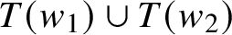 $T(w_1) \cup T(w_2)$
can be smoothed to
$T(w_1) \cup T(w_2)$
can be smoothed to
 $T(w_1 + w_2)$
(observed by Mirzakhani in [Reference Mirzakhani42, Appendix A] and the second author in [55, Subsection 3.2]).
$T(w_1 + w_2)$
(observed by Mirzakhani in [Reference Mirzakhani42, Appendix A] and the second author in [55, Subsection 3.2]).
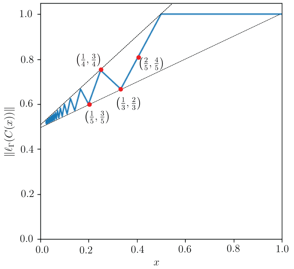
Figure 4.2 We consider the curve
 $C(x)$
carried by a train track depending on a parameter x and plot the stable word length of
$C(x)$
carried by a train track depending on a parameter x and plot the stable word length of
 $C(x)$
as a function of x. The graph has vertices at
$C(x)$
as a function of x. The graph has vertices at
 $\big (\frac {1}{2n+1},\frac {n+1}{2n+1}\big )$
and
$\big (\frac {1}{2n+1},\frac {n+1}{2n+1}\big )$
and
 $ \big (\frac {1}{2n},\frac {n+1}{2n}\big )$
.
$ \big (\frac {1}{2n},\frac {n+1}{2n}\big )$
.
4.6 Asymmetric lengths
The arguments in Subsection 4.5 apply equally well to cases where distances may be zero or not symmetric. For instance, we can take a directed graph
 $\Gamma $
with a nonnegative length on each edge, together with a map
$\Gamma $
with a nonnegative length on each edge, together with a map
 $\iota \colon \Gamma \to S$
so that the corresponding cover
$\iota \colon \Gamma \to S$
so that the corresponding cover
 $\widetilde {\Gamma }$
is strongly connected (every vertex can be reached from any other vertex). The same arguments apply to show that
$\widetilde {\Gamma }$
is strongly connected (every vertex can be reached from any other vertex). The same arguments apply to show that
 $\ell _\Gamma (\vec C)$
satisfies the oriented quasi-smoothing property and so its stabilisation
$\ell _\Gamma (\vec C)$
satisfies the oriented quasi-smoothing property and so its stabilisation
 ${\lVert } \ell _\Gamma {\rVert }$
extends to a continuous function
${\lVert } \ell _\Gamma {\rVert }$
extends to a continuous function
 $\mathcal {GC}^+(S) \to \mathbb {R}_{\ge 0}$
.
$\mathcal {GC}^+(S) \to \mathbb {R}_{\ge 0}$
.
One example would be to take a generating set for
 $\pi _1(S)$
as a monoid. This corresponds to taking
$\pi _1(S)$
as a monoid. This corresponds to taking
 $\Gamma $
to be a graph with a single vertex and one edge for each monoid generator.
$\Gamma $
to be a graph with a single vertex and one edge for each monoid generator.
4.7 Generalised translation lengths from higher representations
Let G be a real, connected, noncompact, semi-simple, linear Lie group. Let K denote a maximal compact subgroup of G, so that
 $X=G/K$
is the Riemannian symmetric space of G. Let
$X=G/K$
is the Riemannian symmetric space of G. Let
 $[P]$
be the conjugacy class of a parabolic subgroup
$[P]$
be the conjugacy class of a parabolic subgroup
 $P \subset G$
. Then there is a natural notion of
$P \subset G$
. Then there is a natural notion of
 $[P]$
-Anosov representation
$[P]$
-Anosov representation
 $\rho \colon \pi _1(S) \to G$
; see, for example, Kassel’s notes [Reference Kassel34, Section 4]. When
$\rho \colon \pi _1(S) \to G$
; see, for example, Kassel’s notes [Reference Kassel34, Section 4]. When
 $\operatorname {rank}_{\mathbb {R}}(G)=1$
there is essentially one class
$\operatorname {rank}_{\mathbb {R}}(G)=1$
there is essentially one class
 $[P]$
, so we can simply refer to them as Anosov representations, and they can be defined as those injective representations
$[P]$
, so we can simply refer to them as Anosov representations, and they can be defined as those injective representations
 $\rho \colon \pi _1(S) \to G$
where
$\rho \colon \pi _1(S) \to G$
where
 $\Gamma := \rho (\pi _1(S))$
preserves and acts cocompactly on some nonempty convex subset V of X.
$\Gamma := \rho (\pi _1(S))$
preserves and acts cocompactly on some nonempty convex subset V of X.
Rank
 $1$
Anosov representations include two familiar examples:
$1$
Anosov representations include two familiar examples:
-
(1) Fuchsian representations into
$G=\operatorname {\mathrm {\mathit {PSL}}}(2,\mathbb {R})$
. Here,
$K=\operatorname {\mathrm {\mathit {SO}}}(2)$
and
$X=\mathbb {H}^2$
. The convex set V in this case is the lift of the convex core of the hyperbolic surface. -
(2) Quasi-Fuchsian representations of surface groups into
$G=\operatorname {\mathrm {\mathit {PSL}}}(2,\mathbb {C})$
. In this case,
$K=\operatorname {\mathrm {\mathit {SU}}}(2)$
,
$X=\mathbb {H}^3$
, and V is the lift of the convex core of the hyperbolic quasi-Fuchsian manifold.

In general, the conjugacy classes of parabolic subgroups of G correspond to subsets
 $\theta $
of the set of restricted simple roots
$\theta $
of the set of restricted simple roots
 $\Delta $
of G. For a given
$\Delta $
of G. For a given
 $[P]$
-Anosov representation and each
$[P]$
-Anosov representation and each
 $\alpha \in \theta $
, Martone and Zhang define [Reference Martone and Zhang38, Definition 2.21] a curve functional
$\alpha \in \theta $
, Martone and Zhang define [Reference Martone and Zhang38, Definition 2.21] a curve functional
 $$ \begin{align*} l_{\alpha}^{\rho}\colon \mathcal{C}(S) \to \mathbb{R}_{\geq 0} \end{align*} $$
and show that for a certain subset of Anosov representations, these can be extended to geodesic currents as intersection numbers with some fixed geodesic current.
For the two rank 1 examples above, this length
 $l_{\alpha }^{\rho }(C)$
corresponds to hyperbolic length of the closed geodesic in the homotopy class C in the quotient hyperbolic manifold
$l_{\alpha }^{\rho }(C)$
corresponds to hyperbolic length of the closed geodesic in the homotopy class C in the quotient hyperbolic manifold
 $\mathbb {H}^2/\rho (\pi _1(S))$
or
$\mathbb {H}^2/\rho (\pi _1(S))$
or
 $\mathbb {H}^3/\rho (\pi _1(S))$
.
$\mathbb {H}^3/\rho (\pi _1(S))$
.
Bonahon showed the length in the Fuchsian case extends to geodesic currents [Reference Bonahon8, Proposition 14]. Our techniques give an extension to geodesic currents of the quasi-fuchsian length; that is, the hyperbolic length of the geodesic representatives in the quasi-Fuchsian manifold.
Proposition 4.11. Translation length
 $l_{\rho }$
, for
$l_{\rho }$
, for
 $\rho \colon \pi _1(S) \to \operatorname {\mathrm {\mathit {PSL}}}(2,\mathbb {C})$
a quasi-Fuchsian representation, extends to geodesic currents.
$\rho \colon \pi _1(S) \to \operatorname {\mathrm {\mathit {PSL}}}(2,\mathbb {C})$
a quasi-Fuchsian representation, extends to geodesic currents.
Proof. Let V to be the convex core of
 $\mathbb {H}^3/\rho (\pi _1(S))$
. We have an obvious retract
$\mathbb {H}^3/\rho (\pi _1(S))$
. We have an obvious retract
 $r\colon V \to S$
(defined up to homotopy). Now use Proposition 4.5, taking
$r\colon V \to S$
(defined up to homotopy). Now use Proposition 4.5, taking
 $\iota =r$
.
$\iota =r$
.
Question 4.12. Bridgeman and Taylor show that a complex length function of a quasi-Fuchsian representation coming from a Patterson–Sullivan measure also extends continuously to a function on geodesic currents, as [Reference Bridgeman and Taylor12, Section 6]. Is there a version of our main theorem that would prove that a complex-valued curve functional like this extends to currents?
Remark 4.13. Extending the definition of convex cocompact representation for higher rank groups turns out to yield products of representations of rank
 $1$
(see Kleiner–Leeb [Reference Kleiner and Leeb35, Theorem 1.3] and Quint [Reference Quint50, Théorème]) so it is not clear that the approach using Proposition 4.5 will allow one to extend curve functionals in higher rank to geodesic currents.
$1$
(see Kleiner–Leeb [Reference Kleiner and Leeb35, Theorem 1.3] and Quint [Reference Quint50, Théorème]) so it is not clear that the approach using Proposition 4.5 will allow one to extend curve functionals in higher rank to geodesic currents.
For
 $G = \operatorname {\mathrm {\mathit {PSL}}}(3,\mathbb {R})$
, there is another cocompact action, not on a convex subset of the symmetric space but on a convex subset of
$G = \operatorname {\mathrm {\mathit {PSL}}}(3,\mathbb {R})$
, there is another cocompact action, not on a convex subset of the symmetric space but on a convex subset of
 $G/P=\mathbb {R}P^2$
. In this case, there is a natural metric on this convex subset, the Hilbert metric. One can easily show using this metric that smoothing is satisfied. In general, in higher rank one can construct similar cocompact actions on convex domains of
$G/P=\mathbb {R}P^2$
. In this case, there is a natural metric on this convex subset, the Hilbert metric. One can easily show using this metric that smoothing is satisfied. In general, in higher rank one can construct similar cocompact actions on convex domains of
 $G/P$
(see Guichard–Wienhard [Reference Guichard and Wienhard28]), but there is not a known canonical choice of metric. Martone and Zhang show [Reference Martone and Zhang38, Theorem 2.1] that some types of representations known as positively ratioed can be realised as intersection numbers with a distinguished geodesic current. This immediately implies this subclass of representations satisfy the smoothing property. It would be interesting to subsume their extension result under our scope. More specifically, we have the following.
$G/P$
(see Guichard–Wienhard [Reference Guichard and Wienhard28]), but there is not a known canonical choice of metric. Martone and Zhang show [Reference Martone and Zhang38, Theorem 2.1] that some types of representations known as positively ratioed can be realised as intersection numbers with a distinguished geodesic current. This immediately implies this subclass of representations satisfy the smoothing property. It would be interesting to subsume their extension result under our scope. More specifically, we have the following.
Question 4.14. Can we prove quasi-smoothing for the translation length for a subclass of
 $[P]$
-Anosov representations, as in Martone–Zhang [Reference Martone and Zhang38, Definition 2.25], directly from the definition of translation length?
$[P]$
-Anosov representations, as in Martone–Zhang [Reference Martone and Zhang38, Definition 2.25], directly from the definition of translation length?
4.8 Extremal length
We now turn to curve functionals that satisfy only convex union and not additive union, starting with the original motivation for this work, extremal length.
Definition 4.15. Fix
 $\Sigma $
a Riemann surface with a metric g. Let
$\Sigma $
a Riemann surface with a metric g. Let
 $C = \bigcup t_iC_i$
be a weighted multi-curve on
$C = \bigcup t_iC_i$
be a weighted multi-curve on
 $\Sigma $
. For
$\Sigma $
. For
 $\rho \colon \Sigma \to \mathbb {R}_{\ge 0}$
a measurable rescaling function, the area of
$\rho \colon \Sigma \to \mathbb {R}_{\ge 0}$
a measurable rescaling function, the area of
 $\rho $
is
$\rho $
is
 $$ \begin{align*} \operatorname{\mathrm{Area}}(\rho g) := \int_{x \in \Sigma} \rho(x)^2 \mu_g(x), \end{align*} $$
where
 $\mu _g$
is the Lebesgue measure of g. The length of C is
$\mu _g$
is the Lebesgue measure of g. The length of C is
 $$ \begin{align*} \ell_{\rho g}(C) := \inf_{\gamma \in C} \sum_i t_i \int_{x\in\gamma_i} \rho(x)\,dx, \end{align*} $$
where
 $dx$
is measured with respect to g arc-length and the infimum runs overall all representatives
$dx$
is measured with respect to g arc-length and the infimum runs overall all representatives
 $\gamma = \bigcup _i \gamma _i$
of C, where
$\gamma = \bigcup _i \gamma _i$
of C, where
 $\gamma _i$
is a representative of the component
$\gamma _i$
is a representative of the component
 $C_i$
of C. When
$C_i$
of C. When
 $\rho $
is continuous,
$\rho $
is continuous,
 $\ell _\rho (C)$
is the length with respect to the metric g rescaled by
$\ell _\rho (C)$
is the length with respect to the metric g rescaled by
 $\rho $
. The square root of the extremal length of C is
$\rho $
. The square root of the extremal length of C is
 $$ \begin{align*} \sqrt{\operatorname{\mathrm{EL}}}(C) := \mathop{\mathrm{sup}}\limits_\rho \frac{\ell_{\rho g}(C)}{\sqrt{\operatorname{\mathrm{Area}}(\rho g)}}. \end{align*} $$
Observe that the supremand is unchanged under multiplying
 $\rho $
by a positive constant. It is a standard result that the supremum is realised by some generalised metric (not necessarily Riemannian) [Reference Tyrell Rockafellar52, Theorem 12] and that, when C is a simple multi-curve, the optimum metric
$\rho $
by a positive constant. It is a standard result that the supremum is realised by some generalised metric (not necessarily Riemannian) [Reference Tyrell Rockafellar52, Theorem 12] and that, when C is a simple multi-curve, the optimum metric
 $\rho g$
is the cone Euclidean metric associated to a quadratic differential, as shown by Jenkins [Reference Jenkins33]. Very little is known about the optimum metric when C is not simple, except in special cases [Reference Wolf and Zwiebach62, Reference Calabi14, Reference Headrick and Zwiebach31, Reference Naseer and Zwiebach46].
$\rho g$
is the cone Euclidean metric associated to a quadratic differential, as shown by Jenkins [Reference Jenkins33]. Very little is known about the optimum metric when C is not simple, except in special cases [Reference Wolf and Zwiebach62, Reference Calabi14, Reference Headrick and Zwiebach31, Reference Naseer and Zwiebach46].
Lemma 4.16. As a function of C with fixed
 $\Sigma $
,
$\Sigma $
,
 $\sqrt {\operatorname {\mathrm {EL}}}$
satisfies homogeneity, stability and smoothing.
$\sqrt {\operatorname {\mathrm {EL}}}$
satisfies homogeneity, stability and smoothing.
Proof. This follows since
 $\ell _{\rho g}$
satisfies these properties for each
$\ell _{\rho g}$
satisfies these properties for each
 $\rho $
; here is the argument for smoothing.
$\rho $
; here is the argument for smoothing.
Let C be a multi-curve with an essential crossing and let
 $C'$
be the curve obtained by smoothing at the crossing. Then, for any scaling function
$C'$
be the curve obtained by smoothing at the crossing. Then, for any scaling function
 $\rho $
,
$\rho $
,
 $$ \begin{align*} \frac{\ell_{\rho g}(C')}{\sqrt{\operatorname{\mathrm{Area}}(\rho g)}} \le \frac{\ell_{\rho g}(C)}{\sqrt{\operatorname{\mathrm{Area}}(\rho g)}}. \end{align*} $$
Since
 $\sqrt {\operatorname {\mathrm {EL}}}(C')$
and
$\sqrt {\operatorname {\mathrm {EL}}}(C')$
and
 $\sqrt {\operatorname {\mathrm {EL}}(C)}$
are the suprema of such terms, the result follows.
$\sqrt {\operatorname {\mathrm {EL}}(C)}$
are the suprema of such terms, the result follows.
Convex union is different, since on one side of the inequality we have a sum of values of
 $\sqrt {\operatorname {\mathrm {EL}}}$
. (Extremal length does not satisfy additivity.)
$\sqrt {\operatorname {\mathrm {EL}}}$
. (Extremal length does not satisfy additivity.)
Lemma 4.17.
 $\sqrt {\operatorname {\mathrm {EL}}}$
satisfies convex union.
$\sqrt {\operatorname {\mathrm {EL}}}$
satisfies convex union.
Proof. Fix a curve split as a union
 $C = C_1 \cup C_2$
, and let
$C = C_1 \cup C_2$
, and let
 $\rho \colon \Sigma \to \mathbb {R}$
be the function realising the supremum in the definition of extremal length for C. Then
$\rho \colon \Sigma \to \mathbb {R}$
be the function realising the supremum in the definition of extremal length for C. Then
 $$ \begin{align*} \sqrt{\operatorname{\mathrm{EL}}}(C_1 \cup C_2) &= \frac{\ell_{\rho g}(C_1)}{\sqrt{\operatorname{\mathrm{Area}}(\rho g)}} + \frac{\ell_{\rho g}(C_2)}{\sqrt{\operatorname{\mathrm{Area}}(\rho g)}}\\ &\le \sqrt{\operatorname{\mathrm{EL}}}(C_1) + \sqrt{\operatorname{\mathrm{EL}}}(C_2), \end{align*} $$
where the last inequality holds by the supremum in the definition of
 $\operatorname {\mathrm {EL}}$
.
$\operatorname {\mathrm {EL}}$
.
Thus, by Theorem A,
 $\sqrt {\operatorname {\mathrm {EL}}}$
(and
$\sqrt {\operatorname {\mathrm {EL}}}$
(and
 $\operatorname {\mathrm {EL}}$
) extend uniquely to continuous functions on geodesic currents. With this extension, we propose the following conjecture.
$\operatorname {\mathrm {EL}}$
) extend uniquely to continuous functions on geodesic currents. With this extension, we propose the following conjecture.
Conjecture 4.18. For some universal constant C,
 $$ \begin{align*}\operatorname{\mathrm{EL}}_{\Sigma}(\mathcal{L}_{\Sigma})=C\operatorname{\mathrm{Area}}(\Sigma),\end{align*} $$
where
 $\mathcal {L}_{\Sigma }$
is the Liouville current (compare Subsection 4.2).
$\mathcal {L}_{\Sigma }$
is the Liouville current (compare Subsection 4.2).
Remark 4.19. For the extremal length without the square root, we instead have inequalities
 $$ \begin{align*} \operatorname{\mathrm{EL}}(C_1) + \operatorname{\mathrm{EL}}(C_2) \le \operatorname{\mathrm{EL}}(C_1 \cup C_2) \le 2(\operatorname{\mathrm{EL}}(C_1) + \operatorname{\mathrm{EL}}(C_2)). \end{align*} $$
The second inequality is a simple consequence of Lemma 4.17. To see the first inequality, take optimal rescaling functions
 $\rho _i$
for
$\rho _i$
for
 $\operatorname {\mathrm {EL}}(C_i)$
, normalised so that
$\operatorname {\mathrm {EL}}(C_i)$
, normalised so that
 $\ell _{\rho _i g}(C_i) = \operatorname {\mathrm {Area}}(\rho _i g) = \operatorname {\mathrm {EL}}(C_i)$
. Then using
$\ell _{\rho _i g}(C_i) = \operatorname {\mathrm {Area}}(\rho _i g) = \operatorname {\mathrm {EL}}(C_i)$
. Then using
 $\rho _1 + \rho _2$
as the test function for
$\rho _1 + \rho _2$
as the test function for
 $\operatorname {\mathrm {EL}}(C_1 \cup C_2)$
gives the desired inequality after elementary manipulations.
$\operatorname {\mathrm {EL}}(C_1 \cup C_2)$
gives the desired inequality after elementary manipulations.
4.9 Extremal length with respect to elastic graphs
There is a parallel notion of extremal length with respect to elastic graphs, as introduced by the second author [Reference Thurston56], just as there is for ordinary lengths (Subsection 4.4).
An elastic graph
 $(\Gamma ,\alpha )$
is a 1-dimensional CW complex
$(\Gamma ,\alpha )$
is a 1-dimensional CW complex
 $\Gamma $
(i.e., allowing multiple edges and loops) together with an assignment of positive real numbers
$\Gamma $
(i.e., allowing multiple edges and loops) together with an assignment of positive real numbers
 $\alpha (e)$
for each
$\alpha (e)$
for each
 $e \in \operatorname {Edge}(\Gamma )$
, where the edges are the 1-dimensional cells of
$e \in \operatorname {Edge}(\Gamma )$
, where the edges are the 1-dimensional cells of
 $\Gamma $
.
$\Gamma $
.
By a concrete multi-curve
 $\gamma $
on
$\gamma $
on
 $\Gamma $
we mean a 1-manifold
$\Gamma $
we mean a 1-manifold
 $X(\gamma )$
and a PL map
$X(\gamma )$
and a PL map
 $\gamma \colon X(\gamma ) \to \Gamma $
. Given a scaling function
$\gamma \colon X(\gamma ) \to \Gamma $
. Given a scaling function
 $\rho \colon \operatorname {Edge}(\Gamma ) \to \mathbb {R}_{\geq 0}$
, the length metric
$\rho \colon \operatorname {Edge}(\Gamma ) \to \mathbb {R}_{\geq 0}$
, the length metric
 $\rho \alpha $
on
$\rho \alpha $
on
 $\Gamma $
gives edge e the length
$\Gamma $
gives edge e the length
 $\rho (e)\alpha (e)$
. We define the length of
$\rho (e)\alpha (e)$
. We define the length of
 $\gamma $
as
$\gamma $
as
 $$ \begin{align*} \ell_{\rho \alpha}(\gamma) := \sum_{e \in \operatorname{Edge}(\Gamma)} n_\gamma(e)\rho(e)\alpha(e), \end{align*} $$
where
 $n_\gamma (e)$
is the weighted number of times that
$n_\gamma (e)$
is the weighted number of times that
 $\gamma $
runs over e. We can likewise define the length of a multi-curve D on
$\gamma $
runs over e. We can likewise define the length of a multi-curve D on
 $\Gamma $
as the infimum over of concrete multi-curves in D.
$\Gamma $
as the infimum over of concrete multi-curves in D.
The area of
 $\Gamma $
with respect to
$\Gamma $
with respect to
 $\rho \alpha $
is defined to be
$\rho \alpha $
is defined to be
 $$ \begin{align*} \operatorname{\mathrm{Area}}_{\rho}(\Gamma,\alpha) := \sum_{e \in \operatorname{Edge}(\Gamma)} \rho(e)^2 \alpha(e). \end{align*} $$
Intuitively, each edge is turned into a rectangle of width
 $\rho (e)$
, aspect ratio
$\rho (e)$
, aspect ratio
 $\alpha (e)$
and thus area
$\alpha (e)$
and thus area
 $\rho (e)^2\alpha (e)$
.
$\rho (e)^2\alpha (e)$
.
As for extremal length for surfaces, we define the square root of extremal length of a multi-curve on
 $\Gamma $
by
$\Gamma $
by
 $$ \begin{align} \sqrt{\operatorname{\mathrm{EL}}}(D; \Gamma,\alpha) := \mathop{\mathrm{sup}}\limits_{ \rho : \operatorname{Edge}(\Gamma) \to \mathbb{R}_{\geq 0}} \frac{\ell_{\rho \alpha}(D)}{\sqrt{\operatorname{\mathrm{Area}}_{\rho}(\Gamma,\alpha)}}. \end{align} $$
It is easy to do this optimisation. We get a more interesting quantity by incorporating a filling embedding
 $\iota \colon \Gamma \hookrightarrow S$
of
$\iota \colon \Gamma \hookrightarrow S$
of
 $\Gamma $
in a surface S; that is, an embedding
$\Gamma $
in a surface S; that is, an embedding
 $\iota $
that is
$\iota $
that is
 $\pi _1$
-surjective. Then, for a multi-curve C on S and scaling
$\pi _1$
-surjective. Then, for a multi-curve C on S and scaling
 $\rho $
, the length is defined as in Subsection 4.4:
$\rho $
, the length is defined as in Subsection 4.4:
 $$ \begin{align*} \ell_{\rho\alpha;\iota}(C) := \inf_{\substack{D\text{ on }\Gamma\\\iota_*(D) = C}} \ell_{\rho\alpha}(D). \end{align*} $$
(The ‘filling’ condition guarantees that there are such multi-curves D with
 $\iota _*(D) = C$
.) We can then define a version of extremal length, following equation (4.20), with respect to
$\iota _*(D) = C$
.) We can then define a version of extremal length, following equation (4.20), with respect to
 $\iota $
:
$\iota $
:
 $$ \begin{align} \sqrt{\operatorname{\mathrm{EL}}}(C; \Gamma,\alpha,\iota) := \mathop{\mathrm{sup}}\limits_{ \rho : \operatorname{Edge}(\Gamma) \to \mathbb{R}_{\geq 0}} \frac{\ell_{\rho \alpha;\iota}(D)}{\sqrt{\operatorname{\mathrm{Area}}_{\rho}(\Gamma,\alpha)}}. \end{align} $$
Proposition 4.22. For
 $\iota \colon \Gamma \to \Sigma $
a filling embedding,
$\iota \colon \Gamma \to \Sigma $
a filling embedding,
 $\sqrt {\operatorname {\mathrm {EL}}}(C; \Gamma ,\alpha ,\iota )$
satisfies the convex union, stability, homogeneity and smoothing properties.
$\sqrt {\operatorname {\mathrm {EL}}}(C; \Gamma ,\alpha ,\iota )$
satisfies the convex union, stability, homogeneity and smoothing properties.
Proof. As in Lemma 4.16, smoothing, stability and homogeneity follow because
 $\ell _{\rho \alpha }(C)$
satisfies them for any
$\ell _{\rho \alpha }(C)$
satisfies them for any
 $\rho $
. Convex union follows as in Lemma 4.17.
$\rho $
. Convex union follows as in Lemma 4.17.
We can also consider extremal length with respect to an immersion
 $\iota $
(rather than an embedding), defined in the same way.
$\iota $
(rather than an embedding), defined in the same way.
Proposition 4.23. For
 $\iota \colon \Gamma \to \Sigma $
a
$\iota \colon \Gamma \to \Sigma $
a
 $\pi _1$
-surjective immersion,
$\pi _1$
-surjective immersion,
 $\sqrt {\operatorname {\mathrm {EL}}}(C; \Gamma , \alpha , \iota )$
satisfies the convex union, homogeneity and quasi-smoothing properties.
$\sqrt {\operatorname {\mathrm {EL}}}(C; \Gamma , \alpha , \iota )$
satisfies the convex union, homogeneity and quasi-smoothing properties.
Proof. Convex union and homogeneity still hold by the same argument. We need an extra argument for quasi-smoothing. Instead of taking the supremum over all
 $\rho $
, rewrite equation (4.21) as
$\rho $
, rewrite equation (4.21) as
 $$ \begin{align*} \sqrt{\operatorname{\mathrm{EL}}}(C; \Gamma, \alpha, \iota) = \mathop{\mathrm{sup}}\limits_{\substack{\rho : \operatorname{Edge}(\Gamma) \to \mathbb{R}_{\ge 0}\\ \operatorname{Area}_\rho(\Gamma,\alpha) = 1}} \ell_{\rho\alpha}(C). \end{align*} $$
The immersed graph
 $\iota (\Gamma )$
has finitely many self-intersections. For each self-intersection x, take the supremum over the compact set of metrics
$\iota (\Gamma )$
has finitely many self-intersections. For each self-intersection x, take the supremum over the compact set of metrics
 $\{\rho \mid \operatorname {\mathrm {Area}}_\rho (\Gamma ,\alpha ) = 1\}$
of the diameter
$\{\rho \mid \operatorname {\mathrm {Area}}_\rho (\Gamma ,\alpha ) = 1\}$
of the diameter
 $\operatorname {\mathrm {diam}}_\iota (x)$
defined in equation (4.7). By the replacement argument in Proposition 4.5, all
$\operatorname {\mathrm {diam}}_\iota (x)$
defined in equation (4.7). By the replacement argument in Proposition 4.5, all
 $\ell _{\rho \alpha }$
for
$\ell _{\rho \alpha }$
for
 $\rho $
in this set satisfy quasi-smoothing with a uniform quasi-smoothing constant. It follows that
$\rho $
in this set satisfy quasi-smoothing with a uniform quasi-smoothing constant. It follows that
 $\operatorname {\mathrm {EL}}(C; \Gamma ,\alpha ,\iota )$
also satisfies quasi-smoothing with the same constant.
$\operatorname {\mathrm {EL}}(C; \Gamma ,\alpha ,\iota )$
also satisfies quasi-smoothing with the same constant.
Remark 4.24. We can relate extremal length for elastic graphs and surfaces by making a choice of a ribbon structure to
 $\Gamma $
. Given any
$\Gamma $
. Given any
 $\varepsilon>0$
, a ribbon elastic graph G can be thickened into a conformal surface with boundary
$\varepsilon>0$
, a ribbon elastic graph G can be thickened into a conformal surface with boundary
 $N_{\varepsilon }(G)$
by replacing each edge e of G by a rectangle of size
$N_{\varepsilon }(G)$
by replacing each edge e of G by a rectangle of size
 $\alpha (e) \times \varepsilon $
and gluing the rectangles at the vertices by using the given ribbon structure. There are then inequalities relating
$\alpha (e) \times \varepsilon $
and gluing the rectangles at the vertices by using the given ribbon structure. There are then inequalities relating
 $\operatorname {\mathrm {EL}}(C; \Gamma ,\alpha )$
and
$\operatorname {\mathrm {EL}}(C; \Gamma ,\alpha )$
and
 $\varepsilon \operatorname {\mathrm {EL}}(C;N_{\varepsilon }(G))$
, to within a multiplicative factor as shown by the second author [Reference Thurston57, Props. 4.8 and 4.9]. For graphs immersed or embedded in a surface, the situation is less clear. By suitably choosing the elastic weights on an embedded graph, it appears that one can approximate extremal length well; Palmer gives one approach [Reference Palmer48]. We are not aware of precise theorems.
$\varepsilon \operatorname {\mathrm {EL}}(C;N_{\varepsilon }(G))$
, to within a multiplicative factor as shown by the second author [Reference Thurston57, Props. 4.8 and 4.9]. For graphs immersed or embedded in a surface, the situation is less clear. By suitably choosing the elastic weights on an embedded graph, it appears that one can approximate extremal length well; Palmer gives one approach [Reference Palmer48]. We are not aware of precise theorems.
4.10 p-Extremal-length with respect to immersed graphs
Extremal length fits into a family of energies for graphs, as explored by the second author in [Reference Thurston56, Appendix A]. For
 $\Gamma $
a metric graph with metric g, a constant p with
$\Gamma $
a metric graph with metric g, a constant p with
 $1 \le p \le \infty $
and C a curve on
$1 \le p \le \infty $
and C a curve on
 $\Gamma $
, define
$\Gamma $
, define
 $$ \begin{align} E_p(C;\Gamma,g) :=\! \mathop{\mathrm{sup}}\limits_{\sigma:\operatorname{Edge}(\Gamma) \to \mathbb{R}_{\ge 0}} \frac{\ell(C; \sigma g)}{{\lVert} \sigma {\rVert}_p} \end{align} $$
where the
 $L^p$
norm
$L^p$
norm
 ${\lVert } \sigma {\rVert }_p$
is taken with respect to the metric g. As in the previous section, we can also consider a
${\lVert } \sigma {\rVert }_p$
is taken with respect to the metric g. As in the previous section, we can also consider a
 $\pi _1$
-surjective immersion
$\pi _1$
-surjective immersion
 $\iota \colon \Gamma \to S$
and consider C to be a curve on S rather than on
$\iota \colon \Gamma \to S$
and consider C to be a curve on S rather than on
 $\Gamma $
.
$\Gamma $
.
For
 $p=\infty $
,
$p=\infty $
,
 $E_\infty (C)$
is in fact just the length with respect to g (as in Subsection 4.5). Indeed, let
$E_\infty (C)$
is in fact just the length with respect to g (as in Subsection 4.5). Indeed, let
 $\sigma $
be any scaling factor, and let
$\sigma $
be any scaling factor, and let
 $\gamma $
be the shortest representative of C on
$\gamma $
be the shortest representative of C on
 $\Gamma $
with respect to g (not with respect to
$\Gamma $
with respect to g (not with respect to
 $\sigma g$
). Then
$\sigma g$
). Then
 $$ \begin{align*} \ell(C; \sigma g) \le \ell(\gamma; \sigma g) \le {\lVert} \sigma {\rVert}_\infty \ell(\gamma; g), \end{align*} $$
from which the result easily follows.
Proposition 4.26. For any
 $\pi _1$
-surjective immersion
$\pi _1$
-surjective immersion
 $\iota \colon \Gamma \to S$
, the curve functional
$\iota \colon \Gamma \to S$
, the curve functional
 $E_p(\cdot; \Gamma , g, \iota )$
satisfies convex union, homogeneity and quasi-smoothing, and thus its stabilisation extends continuously to a function on geodesic currents. If
$E_p(\cdot; \Gamma , g, \iota )$
satisfies convex union, homogeneity and quasi-smoothing, and thus its stabilisation extends continuously to a function on geodesic currents. If
 $\iota $
is a filling embedding, then
$\iota $
is a filling embedding, then
 $E_p$
in addition satisfies stability and smoothing.
$E_p$
in addition satisfies stability and smoothing.

5 Counting problems
One direct application of Theorem A is to obtain new counting results for curves on surfaces of a given topological type.
A filling current is a geodesic current
 $\alpha \in \mathcal {G}\mathcal {C}(\Sigma )$
so that
$\alpha \in \mathcal {G}\mathcal {C}(\Sigma )$
so that
 $i(\alpha ,\mu )>0$
for all
$i(\alpha ,\mu )>0$
for all
 $\mu \in \mathcal {G}\mathcal {C}(\Sigma )\backslash \{ 0 \}$
. One example is a filling multi-curve, one whose complement in S consists of disks.
$\mu \in \mathcal {G}\mathcal {C}(\Sigma )\backslash \{ 0 \}$
. One example is a filling multi-curve, one whose complement in S consists of disks.
Rafi and Souto [Reference Rafi and Souto51] proved the following.
Definition 5.1. A function f on currents is positive if
 $f(\mu )> 0$
for all
$f(\mu )> 0$
for all
 $\mu \ne 0$
.
$\mu \ne 0$
.
For a fixed continuous, homogeneous and positive function
 $f\colon \mathcal {GC} \to \mathbb {R}_{+}$
,
$f\colon \mathcal {GC} \to \mathbb {R}_{+}$
,
 $\alpha $
a current and L a positive real number, let
$\alpha $
a current and L a positive real number, let
 $$ \begin{align*}N(f,\alpha,L) := \# \{ \phi \in \operatorname{\mathrm{\mathit{MCG}}} \mid f(\phi(\alpha)) \leq L\}.\end{align*} $$
Theorem 5.2 Rafi-Souto [Reference Rafi and Souto51, Main Theorem]
For a fixed continuous, homogeneous and positive function
 $f\colon \mathcal {GC} \to \mathbb {R}_{+}$
and for a fixed filling current
$f\colon \mathcal {GC} \to \mathbb {R}_{+}$
and for a fixed filling current
 $\alpha \in \mathcal {G}\mathcal {C}(\Sigma )$
, the limit
$\alpha \in \mathcal {G}\mathcal {C}(\Sigma )$
, the limit
 $$ \begin{align*} \lim_{L \to \infty} \frac{N(f,\alpha,L)}{L^{6g-6}} \end{align*} $$
exists and is equal to
 $$ \begin{align*} \frac{m(f)m(\alpha)}{\mathfrak{m}_g} \end{align*} $$
where
 $m(f)$
,
$m(f)$
,
 $m(\alpha )$
and
$m(\alpha )$
and
 $\mathfrak {m}_g$
are constants depending only on f,
$\mathfrak {m}_g$
are constants depending only on f,
 $\alpha $
and the genus g, respectively:
$\alpha $
and the genus g, respectively:
 $$ \begin{align} m(f)&=\mu_{\mathrm{Thu}}(\{\lambda \in \mathcal{ML} \mid f(\lambda) \leq 1 \}) \end{align} $$
 $$ \begin{align} m(\alpha)&=\mu_{\mathrm{Thu}}(\{\lambda \in \mathcal{ML} \mid i(\alpha,\lambda) \leq 1 \}) \end{align} $$
 $$ \begin{align} \mathfrak{m}_g &= \int_{\mathcal{M}_g}\!m(Y)\,d\omega_{\mathrm{WP}}(Y). \end{align} $$
Here
 $\mu _{\mathrm {Thu}}$
is the Thurston measure on
$\mu _{\mathrm {Thu}}$
is the Thurston measure on
 $\mathcal {ML}$
. One way to obtain it is as a scaling limit of Dirac measures on measured laminations supported on integral simple multi-curves (see Erlandsson–Souto’s book [Reference Erlandsson and Souto26, Proposition 8.8]). Another way is as a certain normalisation of the volume form induced by the symplectic structure on measured laminations [Reference Erlandsson and Souto26, Theorem 4.16].
$\mathcal {ML}$
. One way to obtain it is as a scaling limit of Dirac measures on measured laminations supported on integral simple multi-curves (see Erlandsson–Souto’s book [Reference Erlandsson and Souto26, Proposition 8.8]). Another way is as a certain normalisation of the volume form induced by the symplectic structure on measured laminations [Reference Erlandsson and Souto26, Theorem 4.16].
Dumas [Reference Dumas21] communicates a proof of the following theorem (attributed to Mirzakhani).
Theorem 5.6 Dumas–Mirzakhani [Reference Dumas21, Theorem 5.10]
The function
 $\Lambda \colon \mathcal {M}_g \to \mathbb {R}_{\geq 0}$
given by
$\Lambda \colon \mathcal {M}_g \to \mathbb {R}_{\geq 0}$
given by
 $\Sigma \mapsto m(\operatorname {EL}_{\Sigma })$
is constant, where
$\Sigma \mapsto m(\operatorname {EL}_{\Sigma })$
is constant, where
 $m(\operatorname {\mathrm {EL}}_\Sigma )$
is defined by equation (5.3).
$m(\operatorname {\mathrm {EL}}_\Sigma )$
is defined by equation (5.3).
Let
 $\sqrt {\operatorname {EL}_{\Sigma }}\colon \mathcal {GC} \to \mathbb {R}_{\geq 0}$
be the continuous extension of square root of extremal length to currents provided by Theorem A. In order to be able to apply Theorem 5.2, it remains to check that the square root of extremal length is nonzero.
$\sqrt {\operatorname {EL}_{\Sigma }}\colon \mathcal {GC} \to \mathbb {R}_{\geq 0}$
be the continuous extension of square root of extremal length to currents provided by Theorem A. In order to be able to apply Theorem 5.2, it remains to check that the square root of extremal length is nonzero.
Lemma 5.7. For any
 $\Sigma \in \operatorname {\mathrm {Teich}}(S)$
, the functional
$\Sigma \in \operatorname {\mathrm {Teich}}(S)$
, the functional
 $\sqrt {\operatorname {EL}_{\Sigma }}$
is positive on
$\sqrt {\operatorname {EL}_{\Sigma }}$
is positive on
 $\mathcal {GC}(\Sigma )$
.
$\mathcal {GC}(\Sigma )$
.
Proof. Let
 $A = \sqrt {-2\pi \chi (S)}$
. By Definition 4.15 applied to the hyperbolic metric,
$A = \sqrt {-2\pi \chi (S)}$
. By Definition 4.15 applied to the hyperbolic metric,
 $\ell _{\Sigma }(C)/A \leq \sqrt {\operatorname {EL}_{\Sigma }}(C)$
for all curves C and all
$\ell _{\Sigma }(C)/A \leq \sqrt {\operatorname {EL}_{\Sigma }}(C)$
for all curves C and all
 $\Sigma \in \operatorname {\mathrm {Teich}}(S)$
. For any
$\Sigma \in \operatorname {\mathrm {Teich}}(S)$
. For any
 $\mu \in \mathcal {GC}(\Sigma )$
, there exists a sequence
$\mu \in \mathcal {GC}(\Sigma )$
, there exists a sequence
 $(\lambda _i C_i)_{i \in \mathbb {N}}$
of weighted curves so that
$(\lambda _i C_i)_{i \in \mathbb {N}}$
of weighted curves so that
 $\lambda _i C_i \to \mu $
in the weak
$\lambda _i C_i \to \mu $
in the weak
 $^*$
sense. It thus follows that
$^*$
sense. It thus follows that
 $\ell _{\Sigma }(\mu )/A\leq \sqrt {\operatorname {\mathrm {EL}}_\Sigma }(\mu )$
. Since
$\ell _{\Sigma }(\mu )/A\leq \sqrt {\operatorname {\mathrm {EL}}_\Sigma }(\mu )$
. Since
 $\ell _{\Sigma }$
is a positive function on currents,
$\ell _{\Sigma }$
is a positive function on currents,
 $\sqrt {\operatorname {\mathrm {EL}}_\Sigma }$
is as well.
$\sqrt {\operatorname {\mathrm {EL}}_\Sigma }$
is as well.
We thus get solutions to counting problems for extremal length.
Corollary 5.8. For any filling current
 $\alpha $
and
$\alpha $
and
 ${\Sigma } \in \operatorname {\mathrm {Teich}}(S)$
, the limit
${\Sigma } \in \operatorname {\mathrm {Teich}}(S)$
, the limit
 $$ \begin{align*} \lim_{L \to \infty} \frac{N(\sqrt{\operatorname{\mathrm{EL}}_{\Sigma}},\alpha,L)}{L^{6g-6}} \end{align*} $$
exists, is independent of
 $\Sigma $
and is equal to
$\Sigma $
and is equal to
 $$ \begin{align} \frac{\Lambda \cdot m(\alpha)}{\mathfrak{m}_g}. \end{align} $$
Proof. Using Theorem A and the results in Subsection 4.8, we can extend
 $\sqrt {EL_X}$
as a continuous, real-homogeneous functional on geodesic currents. Furthermore,
$\sqrt {EL_X}$
as a continuous, real-homogeneous functional on geodesic currents. Furthermore,
 $\sqrt {EL_X}$
is positive on currents, by Proposition 5.7. Thus, by Theorem 5.2, the result follows. Independence of
$\sqrt {EL_X}$
is positive on currents, by Proposition 5.7. Thus, by Theorem 5.2, the result follows. Independence of
 $\Sigma $
follows from Theorem 5.6.
$\Sigma $
follows from Theorem 5.6.
A similar counting result is true for
 $\alpha $
a simple multi-curve by Mirzakhani’s work, but one has to count slightly differently. For f a curve functional,
$\alpha $
a simple multi-curve by Mirzakhani’s work, but one has to count slightly differently. For f a curve functional,
 $\alpha $
a simple curve and
$\alpha $
a simple curve and
 $L> 0$
, set
$L> 0$
, set
 $$ \begin{align*}n(f,\alpha,L) := \# \{ \phi(\alpha)\in \operatorname{\mathrm{\mathit{MCG}}} \mid f(\phi(\alpha)) \leq L\}.\end{align*} $$
In general, note that
 $n(f,\alpha ,L) \neq N(f,\alpha ,L)$
; in fact, N will be infinite if
$n(f,\alpha ,L) \neq N(f,\alpha ,L)$
; in fact, N will be infinite if
 $\alpha $
is not filling. Even for
$\alpha $
is not filling. Even for
 $\alpha $
filling, N will be bigger than n if
$\alpha $
filling, N will be bigger than n if
 $\alpha $
has nontrivial stabiliser in the mapping class group.
$\alpha $
has nontrivial stabiliser in the mapping class group.
We state the corresponding result for simple multi-curves.
Proposition 5.10. For any simple multi-curve
 $\alpha $
, there is a constant
$\alpha $
, there is a constant
 $c(\alpha )$
so that, for any
$c(\alpha )$
so that, for any
 $f \colon \mathcal {GC}^+(S) \to \mathbb {R}$
continuous, positive and real-homogeneous function, the limit
$f \colon \mathcal {GC}^+(S) \to \mathbb {R}$
continuous, positive and real-homogeneous function, the limit
 $$ \begin{align} \lim_{L \to \infty} \frac{n(f,\alpha,L)}{L^{6g-6}} \end{align} $$
exists and is equal to
 $$ \begin{align} \frac{m(f)c(\alpha)}{\mathfrak{m}_g}. \end{align} $$
Proof. First note that the set
 $\{ \lambda \in \mathcal {ML}(\Sigma ) \mid f(\lambda ) \leq 1 \}$
is compact because f is positive on nonzero measured laminations. Let
$\{ \lambda \in \mathcal {ML}(\Sigma ) \mid f(\lambda ) \leq 1 \}$
is compact because f is positive on nonzero measured laminations. Let
 $A := \{ \lambda \in \mathcal {ML} \mid f(\lambda ) = 1 \})$
; then
$A := \{ \lambda \in \mathcal {ML} \mid f(\lambda ) = 1 \})$
; then
 $\mu _{\mathrm {Thu}}(A)=0$
, as proved by Rafi and Souto [Reference Rafi and Souto51, p. 879]. Finally, we apply Mirzakhani’s counting result [Reference Mirzakhani43, Theorem 1.3] and the Portmanteau theorem (see [Reference Bauer and Burckel6, Theorem 30.12]) to conclude the limit exists.
$\mu _{\mathrm {Thu}}(A)=0$
, as proved by Rafi and Souto [Reference Rafi and Souto51, p. 879]. Finally, we apply Mirzakhani’s counting result [Reference Mirzakhani43, Theorem 1.3] and the Portmanteau theorem (see [Reference Bauer and Burckel6, Theorem 30.12]) to conclude the limit exists.
Corollary 5.13. For any simple multi-curve
 $\alpha $
and
$\alpha $
and
 ${\Sigma } \in \operatorname {\mathrm {Teich}}(S)$
, the limit
${\Sigma } \in \operatorname {\mathrm {Teich}}(S)$
, the limit
 $$ \begin{align*} \lim_{L \to \infty} \frac{n(\sqrt{\operatorname{\mathrm{EL}}_{\Sigma}},\alpha,L)}{L^{6g-6}} \end{align*} $$
exists, is independent of
 $\Sigma $
and is equal to
$\Sigma $
and is equal to
 $$ \begin{align} \frac{\Lambda \cdot c(\alpha)}{\mathfrak{m}_g}. \end{align} $$
Remark 5.15. The constant
 $c(\alpha )$
in Proposition 5.13 is not the same as the constant
$c(\alpha )$
in Proposition 5.13 is not the same as the constant
 $m(\alpha )$
in Theorem 5.2. For details on how
$m(\alpha )$
in Theorem 5.2. For details on how
 $c(\alpha )$
is defined, see Mirzakhani’s paper [Reference Mirzakhani43, Equation (1.2)]. This is related to the fact that in Proposition 5.13 we count multi-curves instead of mapping classes because the stabiliser of a simple multi-curve under the mapping class group is infinite.
$c(\alpha )$
is defined, see Mirzakhani’s paper [Reference Mirzakhani43, Equation (1.2)]. This is related to the fact that in Proposition 5.13 we count multi-curves instead of mapping classes because the stabiliser of a simple multi-curve under the mapping class group is infinite.
The counting problem
 $n(\ell _{\Sigma },\alpha ,L)$
with
$n(\ell _{\Sigma },\alpha ,L)$
with
 $\alpha $
an arbitrary essential multi-curve (possibly neither simple nor filling) and
$\alpha $
an arbitrary essential multi-curve (possibly neither simple nor filling) and
 $f=\ell _{\Sigma }$
a hyperbolic length is established in more recent work of Mirzakhani [Reference Mirzakhani44, Theorem 1.1]. Relying on her work, Erlandsson–Parlier–Souto [Reference Erlandsson, Parlier and Souto23, Theorem 1.6] give the corresponding result where f is allowed to be intersection number with other filling currents (not just a hyperbolic Liouville current). From Mirzakhani’s work and work of Erlandsson–Souto [Reference Erlandsson and Souto24, Corollary 4.4], one also can get the corresponding counting problems where
$f=\ell _{\Sigma }$
a hyperbolic length is established in more recent work of Mirzakhani [Reference Mirzakhani44, Theorem 1.1]. Relying on her work, Erlandsson–Parlier–Souto [Reference Erlandsson, Parlier and Souto23, Theorem 1.6] give the corresponding result where f is allowed to be intersection number with other filling currents (not just a hyperbolic Liouville current). From Mirzakhani’s work and work of Erlandsson–Souto [Reference Erlandsson and Souto24, Corollary 4.4], one also can get the corresponding counting problems where
 $\alpha $
is allowed to be a current (not just a multi-curve). In fact, from Erlandsson–Souto’s work one can also allow f to be any continuous, positive and real-homogeneous function on currents, although they do not explicitly state this in their paper. This is done in Rafi–Souto’s work (Theorem 5.2 above) which also gives the expression (5.9) for the limit of the counting problem. Rafi–Souto also relies on Mirzakhani’s work [Reference Mirzakhani44].
$\alpha $
is allowed to be a current (not just a multi-curve). In fact, from Erlandsson–Souto’s work one can also allow f to be any continuous, positive and real-homogeneous function on currents, although they do not explicitly state this in their paper. This is done in Rafi–Souto’s work (Theorem 5.2 above) which also gives the expression (5.9) for the limit of the counting problem. Rafi–Souto also relies on Mirzakhani’s work [Reference Mirzakhani44].
Finally, recently Erlandsson–Souto [Reference Erlandsson and Souto26, Theorem 8.1] gave an independent proof of the counting argument in [Reference Mirzakhani44] illuminating the connection between counting problems for simple and nonsimple multi-curves. Corollary 5.8 also follows from Proposition 5.13 and forthcoming work of Erlandsson and Souto [Reference Erlandsson and Souto25, Reference Erlandsson and Souto26].
We remark that Erlandsson–Souto’s work shows that if one knows a counting result for simple closed curves, then one can obtain a counting result for nonsimple closed curves (for curve functionals extending continuously to currents). The connection between these two types of counting problems is perhaps that, in some sense, the simple closed curves are the extremal points of the space of currents, in the sense of convex sets [Reference Thurston58]. For instance, the systole of positive curve functional satisfying smoothing and convex union is always a simple curve. (Here by systole we mean a weight
 $1$
, nontrivial multi-curve C with a minimal value of
$1$
, nontrivial multi-curve C with a minimal value of
 $f(C)$
.)
$f(C)$
.)
6 Proof outline
In this section, we prove the core theorem of the article, Theorem 6.1, giving a continuous extension to geodesic currents of a functional f on weighted multi-curves satisfying convex union, stability, homogeneity and weighted quasi-smoothing.
Theorem 6.1. Let f be a weighted curve functional defined on weighted oriented multi-curves satisfying the weighted quasi-smoothing, convex union, stability and homogeneity properties. Then there is a unique continuous homogeneous function
 $\bar {f} \colon \mathcal {GC}^+(S) \to \mathbb {R}_{\ge 0}$
that extends f.
$\bar {f} \colon \mathcal {GC}^+(S) \to \mathbb {R}_{\ge 0}$
that extends f.
Proof of Theorem 6.1. The proof proceeds by studying the geodesic flow on the unit tangent bundle to S (with respect to an arbitrary hyperbolic metric), picking a suitable global cross section with boundary
 $\tau $
and looking at a ‘smeared first return map’ to
$\tau $
and looking at a ‘smeared first return map’ to
 $\tau $
.
$\tau $
.
The proof breaks up into the following steps.
-
• Step 1: In Section 7, we define the cross sections we consider, though we delay proving existence. We introduce bump functions and the associated smeared first return map (Definition 7.4); indeed, there are several varieties of return maps (Table 2). The main advantage of smeared return maps is that they are continuous (Proposition 7.7). We use these smeared returns to define our purported extension
$f_\tau $
to geodesic currents as a limit (Definition 7.25), assuming a suitable global cross section
$\tau $
exists.Table 2 Various types of return maps.
$M = UT\Sigma $
is the domain of the flow
$\phi _t$
. -
• Step 2: In Section 8, we find a suitable ‘good’
$\tau $
, defined in Definition 8.4, by considering certain wedge subsets (Definition 8.1) of
$UT\Sigma $
, based at a collection of geodesic sub-segments of a closed geodesic
$\delta $
(see Proposition 8.3). -
• Step 3: In Section 9, Proposition 9.6, we show the limit defining
$f_\tau $
exists, by using convex union, quasi-smoothing, stability and homogeneity assumptions on f and applying a version of Fekete’s Lemma (Lemma 9.5). -
• Step 4: In Section 10, Proposition 10.8, we show that
$f_{\tau }$
is a continuous function on the space of oriented geodesic currents. We do this by showing that the iterates
$f^k_{\tau }$
used in the definition of
$f_{\tau }$
are continuous for each k, using the continuity of the smeared homotopy return map from Step 1, and f is a continuous function of the weights of a fixed multi-curve (Proposition 3.5). Propositions 9.4 and 10.1 give enough control to ensure uniform convergence of the iterates
$f^k_{\tau }$
to
$f_{\tau }$
(see Lemma 10.2), and thus continuity of
$f_{\tau }$
follows. -
• Step 5: In Section 11, Proposition 11.5, we show that
$f_{\tau }$
extends f for oriented curves, by analysing the image of the smeared return map in that case and mixing and matching the components of the multi-curve.


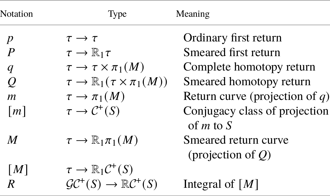


The definition of
 $f_{\tau }$
depends on many choices: the hyperbolic metric on S, a choice of global cross section
$f_{\tau }$
depends on many choices: the hyperbolic metric on S, a choice of global cross section
 $\tau $
and, in fact, nested cross sections
$\tau $
and, in fact, nested cross sections
 $\tau _0 \subset \tau \subset \tau '$
and a choice of bump function
$\tau _0 \subset \tau \subset \tau '$
and a choice of bump function
 $\psi $
on
$\psi $
on
 $\tau $
(see Definition 7.1). Different choices yield, a priori, different extensions
$\tau $
(see Definition 7.1). Different choices yield, a priori, different extensions
 $f_{\tau }$
. But we have proved that
$f_{\tau }$
. But we have proved that
 $f_\tau $
is a continuous function on the space of geodesic currents and, moreover, it restricts to f on multi-curves. Since weighted multi-curves are a dense subset of the space of geodesic currents (see Subsection 2.7), the extension does not depend on these choices. This proves Theorem 6.1.
$f_\tau $
is a continuous function on the space of geodesic currents and, moreover, it restricts to f on multi-curves. Since weighted multi-curves are a dense subset of the space of geodesic currents (see Subsection 2.7), the extension does not depend on these choices. This proves Theorem 6.1.
Now, we prove Theorem A.
7 Defining the extension
We now turn to the proof of Theorem A. As mentioned above, we will fix a hyperbolic structure
 $\Sigma $
on S (with no relation to the curve functional f) and use the geodesic flow
$\Sigma $
on S (with no relation to the curve functional f) and use the geodesic flow
 $\phi _t$
on the unit tangent bundle to define the extension to currents.
$\phi _t$
on the unit tangent bundle to define the extension to currents.
In this section we will deal with return maps for this flow. After some generalities about return maps for cross sections with boundary, we introduce a smeared return map that is continuous. We also define a homotopy return map (and a smeared version of it) that keeps track of homotopy classes of closures of trajectories. Then we use the smeared homotopy return map to define the extension
 $f_\tau $
of f. The several variants of the return map are summarised in Table 2.
$f_\tau $
of f. The several variants of the return map are summarised in Table 2.
7.1 Smeared first return map
Let Y be a smooth closed manifold with a smooth flow
 $\phi _t$
. For us, a cross section is a compact smooth codimension
$\phi _t$
. For us, a cross section is a compact smooth codimension
 $1$
submanifold-with-boundary
$1$
submanifold-with-boundary
 $\tau $
that is smoothly transverse to the foliation of Y given by
$\tau $
that is smoothly transverse to the foliation of Y given by
 $\phi _t$
. A global cross section is a cross section
$\phi _t$
. A global cross section is a cross section
 $\tau $
so that its interior
$\tau $
so that its interior
 $\tau ^\circ $
intersects all forward and backward orbits: for all
$\tau ^\circ $
intersects all forward and backward orbits: for all
 $x \in Y$
, there exists
$x \in Y$
, there exists
 $s<0$
and
$s<0$
and
 $t> 0$
with
$t> 0$
with
 $\phi _s(x), \phi _t(x) \in \tau ^\circ $
. Any flow on a compact manifold has global cross section consisting of a union of finitely many disks, although not all flows on compact manifolds admit a global cross section consisting of a single connected component. (For instance, the Reeb foliation on
$\phi _s(x), \phi _t(x) \in \tau ^\circ $
. Any flow on a compact manifold has global cross section consisting of a union of finitely many disks, although not all flows on compact manifolds admit a global cross section consisting of a single connected component. (For instance, the Reeb foliation on
 $\mathbb {T}^2$
has no connected global cross section.) By the implicit function theorem, for any cross section
$\mathbb {T}^2$
has no connected global cross section.) By the implicit function theorem, for any cross section
 $\tau $
there is a larger cross section
$\tau $
there is a larger cross section
 $\tau '$
with
$\tau '$
with
 $\partial \tau \subset \tau '{}^\circ $
, which we also write
$\partial \tau \subset \tau '{}^\circ $
, which we also write
 $\tau \Subset \tau '$
.
$\tau \Subset \tau '$
.
Let
 $t_\tau \colon Y \to \mathbb {R}$
be the first return time defined by
$t_\tau \colon Y \to \mathbb {R}$
be the first return time defined by
 $t_{\tau }(x):=\min \{ t>0 \mid \phi _t(x) \in \tau \}$
, and let
$t_{\tau }(x):=\min \{ t>0 \mid \phi _t(x) \in \tau \}$
, and let
 $p_{\tau }(x):=\phi _{t_{\tau }(x)}(x)$
. Then
$p_{\tau }(x):=\phi _{t_{\tau }(x)}(x)$
. Then
 $p_{\tau }$
(restricted to
$p_{\tau }$
(restricted to
 $\tau $
) is the first return map associated to the cross section
$\tau $
) is the first return map associated to the cross section
 $\tau $
. We will omit the subscript on
$\tau $
. We will omit the subscript on
 $p_\tau $
if it is clear from context. We also have the first return time to the interior, denoted
$p_\tau $
if it is clear from context. We also have the first return time to the interior, denoted
 $t_\tau ^\circ $
. (Recall we assume
$t_\tau ^\circ $
. (Recall we assume
 $t_\tau ^\circ (x)$
is finite.)
$t_\tau ^\circ (x)$
is finite.)
If
 $\tau $
has no boundary, then p is a homeomorphism. On the other hand, if the cross section has a noninvariant boundary (i.e.,
$\tau $
has no boundary, then p is a homeomorphism. On the other hand, if the cross section has a noninvariant boundary (i.e.,
 $p(\partial \tau ) \ne \partial \tau $
), then
$p(\partial \tau ) \ne \partial \tau $
), then
 $t_\tau $
and p will have discontinuities. This necessarily happens for the geodesic flow on the unit tangent bundle of a hyperbolic surface. See Cossarini–Dehornoy [Reference Cossarini and Dehornoy15, Sec. 1] for a justification and examples of global cross sections with boundary for this flow; we construct our own cross section in Section 8. However, by the continuity of
$t_\tau $
and p will have discontinuities. This necessarily happens for the geodesic flow on the unit tangent bundle of a hyperbolic surface. See Cossarini–Dehornoy [Reference Cossarini and Dehornoy15, Sec. 1] for a justification and examples of global cross sections with boundary for this flow; we construct our own cross section in Section 8. However, by the continuity of
 $\phi _t$
with respect to initial parameters, we have the following ‘local continuity’ claim.
$\phi _t$
with respect to initial parameters, we have the following ‘local continuity’ claim.
Lemma 7.1. Let
 $\tau _1, \tau _2$
be cross sections (not necessarily global) of
$\tau _1, \tau _2$
be cross sections (not necessarily global) of
 $\phi $
. Let
$\phi $
. Let
 $x_1 \in \tau _1^\circ $
, and suppose we are given
$x_1 \in \tau _1^\circ $
, and suppose we are given
 $t> 0$
so
$t> 0$
so
 $x_2=\phi _t(x_1) \in \tau _2^\circ $
. Then there exists a neighbourhood
$x_2=\phi _t(x_1) \in \tau _2^\circ $
. Then there exists a neighbourhood
 $U_1$
of
$U_1$
of
 $x_1$
in
$x_1$
in
 $\tau _1$
, a neighbourhood
$\tau _1$
, a neighbourhood
 $U_2$
of
$U_2$
of
 $x_2$
in
$x_2$
in
 $\tau _2$
and a continuous function
$\tau _2$
and a continuous function
 $t^1_2\colon U_1 \to \mathbb {R}_{>0}$
so that for
$t^1_2\colon U_1 \to \mathbb {R}_{>0}$
so that for
 $x \in U_1$
,
$x \in U_1$
,
 $\phi _{t^1_2}(x) \in U_2$
. Furthermore,
$\phi _{t^1_2}(x) \in U_2$
. Furthermore,
 $\phi _{t^1_2}\colon U_1 \to U_2$
is a diffeomorphism. If t is the first return to
$\phi _{t^1_2}\colon U_1 \to U_2$
is a diffeomorphism. If t is the first return to
 $\tau _2$
, then we can choose
$\tau _2$
, then we can choose
 $U_1$
and
$U_1$
and
 $U_2$
so that
$U_2$
so that
 $t^1_2(x) = t_{\tau _2}(x)$
is also the first return time.
$t^1_2(x) = t_{\tau _2}(x)$
is also the first return time.
This is presumably standard (Basener gives this as ‘a useful technical lemma, the proof of which is trivial’ [Reference Basener3, Lem. 1]), but we give a proof for completeness.
Proof. Pick an initial neighbourhood
 $U_1'$
of
$U_1'$
of
 $x_1$
in
$x_1$
in
 $\tau $
, and let
$\tau $
, and let
 $\varepsilon $
be small enough so that
$\varepsilon $
be small enough so that
 $V_1 := \phi _{(-\varepsilon ,\varepsilon )}(U_1')$
is a 3-dimensional flow-box neighbourhood of
$V_1 := \phi _{(-\varepsilon ,\varepsilon )}(U_1')$
is a 3-dimensional flow-box neighbourhood of
 $x_1$
in Y. Then the restriction of
$x_1$
in Y. Then the restriction of
 $\phi _t$
to
$\phi _t$
to
 $V_1$
is a homeomorphism to a neighbourhood
$V_1$
is a homeomorphism to a neighbourhood
 $V_2$
of
$V_2$
of
 $x_2$
in Y. Set
$x_2$
in Y. Set
 $U_2':= V_2 \cap \tau _2$
. Now consider the composition
$U_2':= V_2 \cap \tau _2$
. Now consider the composition
 $\psi := \pi _1 \circ \phi _{-t} \circ \iota _2 \colon U_2' \to U_1'$
, where
$\psi := \pi _1 \circ \phi _{-t} \circ \iota _2 \colon U_2' \to U_1'$
, where
 $\iota _i \colon U_i' \hookrightarrow V_i$
is the inclusion and
$\iota _i \colon U_i' \hookrightarrow V_i$
is the inclusion and
 $\pi _1 \colon V_1 \to U_1$
is the flow projection:
$\pi _1 \colon V_1 \to U_1$
is the flow projection:

Then
 $\psi $
is a map from
$\psi $
is a map from
 $U_2'$
to
$U_2'$
to
 $U_1'$
, taking
$U_1'$
, taking
 $x_2$
to
$x_2$
to
 $x_1$
. By transversality of
$x_1$
. By transversality of
 $\tau _1$
and
$\tau _1$
and
 $\tau _2$
, the differential of
$\tau _2$
, the differential of
 $\psi $
at
$\psi $
at
 $x_2$
is invertible. Thus, by the inverse function theorem, there is a neighbourhood
$x_2$
is invertible. Thus, by the inverse function theorem, there is a neighbourhood
 $U_2$
of
$U_2$
of
 $x_2$
and
$x_2$
and
 $U_1$
of
$U_1$
of
 $x_1$
so that the restriction of
$x_1$
so that the restriction of
 $\psi $
is a diffeomorphism from
$\psi $
is a diffeomorphism from
 $U_2$
to
$U_2$
to
 $U_1$
. For
$U_1$
. For
 $x \in U_1$
, set
$x \in U_1$
, set
 $t^1_2(x) := t + \pi _t(\phi _{-t}(\psi ^{-1}(x)))$
, where
$t^1_2(x) := t + \pi _t(\phi _{-t}(\psi ^{-1}(x)))$
, where
 $\pi _t \colon V_1 \to (-\varepsilon ,\varepsilon )$
is the projection onto the time coordinate of the flow box. We have
$\pi _t \colon V_1 \to (-\varepsilon ,\varepsilon )$
is the projection onto the time coordinate of the flow box. We have
 $\phi _{t^1_2}(x) = \psi ^{-1}(x) \in U_1$
, as desired for the first claim.
$\phi _{t^1_2}(x) = \psi ^{-1}(x) \in U_1$
, as desired for the first claim.
For the second claim, by hypothesis, the compact sets
 $\phi _{[0,t]}(x_1)$
and
$\phi _{[0,t]}(x_1)$
and
 $\tau _2$
do not intersect, so
$\tau _2$
do not intersect, so
 $\phi _{[0,t]}(x_1)$
has an open neighbourhood that does not intersect
$\phi _{[0,t]}(x_1)$
has an open neighbourhood that does not intersect
 $\tau _2$
. It follows that we can shrink
$\tau _2$
. It follows that we can shrink
 $U_1$
and
$U_1$
and
 $U_2$
so that
$U_2$
so that
 $\psi ^{-1}$
restricted to
$\psi ^{-1}$
restricted to
 $U_1$
is the first return map to
$U_1$
is the first return map to
 $\tau _2$
.
$\tau _2$
.
Lemma 7.2. Let
 $x \in \tau $
. If
$x \in \tau $
. If
 $p(x) \in \tau ^\circ $
, then
$p(x) \in \tau ^\circ $
, then
 $p_\tau $
and
$p_\tau $
and
 $t_\tau $
are continuous in a neighbourhood of x in
$t_\tau $
are continuous in a neighbourhood of x in
 $\tau $
.
$\tau $
.
Proof. Let
 $\tau '\Supset \tau $
be a slightly enlarged global cross section (to cover cases when
$\tau '\Supset \tau $
be a slightly enlarged global cross section (to cover cases when
 $x \in \partial \tau $
). By Lemma 7.1, there exists a neighbourhood U of x in
$x \in \partial \tau $
). By Lemma 7.1, there exists a neighbourhood U of x in
 $\tau '$
such that
$\tau '$
such that
 $p_{\tau }(U) \subset \tau ^\circ $
. By taking
$p_{\tau }(U) \subset \tau ^\circ $
. By taking
 $V:= U \cap \tau $
, we get the desired neighbourhood in
$V:= U \cap \tau $
, we get the desired neighbourhood in
 $\tau $
.
$\tau $
.
Lemma 7.3. Let
 $\tau $
be a global cross section. Then, on
$\tau $
be a global cross section. Then, on
 $\tau $
,
$\tau $
,
 $t_\tau $
is lower semi-continuous and
$t_\tau $
is lower semi-continuous and
 $t_\tau ^\circ $
is upper semi-continuous. There are thus positive global upper and lower bounds on
$t_\tau ^\circ $
is upper semi-continuous. There are thus positive global upper and lower bounds on
 $t_\tau $
.
$t_\tau $
.
Proof. Fix
 $x \in \tau $
. If
$x \in \tau $
. If
 $p_\tau (x) \in \tau ^\circ $
, then
$p_\tau (x) \in \tau ^\circ $
, then
 $t_\tau $
is continuous at x by Lemma 7.2. Otherwise, find a cross section
$t_\tau $
is continuous at x by Lemma 7.2. Otherwise, find a cross section
 $\tau '$
with
$\tau '$
with
 $\tau \Subset \tau '$
. Then
$\tau \Subset \tau '$
. Then
 $t_{\tau '}$
is continuous at x, and since
$t_{\tau '}$
is continuous at x, and since
 $t_\tau (y) \ge t_{\tau '}(y)$
we have proved that
$t_\tau (y) \ge t_{\tau '}(y)$
we have proved that
 $t_\tau $
is lower semi-continuous.
$t_\tau $
is lower semi-continuous.
On the other hand, for any
 $x_1 \in \tau $
, we can set
$x_1 \in \tau $
, we can set
 $x_2=p_\tau ^\circ (x_1)$
and find a neighbourhood
$x_2=p_\tau ^\circ (x_1)$
and find a neighbourhood
 $U_1$
of
$U_1$
of
 $x_1$
in
$x_1$
in
 $\tau $
with a function
$\tau $
with a function
 $t^1_2$
as in Lemma 7.1. But then
$t^1_2$
as in Lemma 7.1. But then
 $t^\circ _\tau (x) \le t^1_2(x)$
for
$t^\circ _\tau (x) \le t^1_2(x)$
for
 $x \in U_1$
. (Note that
$x \in U_1$
. (Note that
 $x_2$
is the first return point to
$x_2$
is the first return point to
 $\tau ^\circ $
, not to
$\tau ^\circ $
, not to
 $\tau $
, so we cannot conclude that
$\tau $
, so we cannot conclude that
 $t_\tau ^\circ $
is continuous.)
$t_\tau ^\circ $
is continuous.)
In the
 $C^1$
setting, Basener showed that a global cross section can be perturbed slightly so that the first return map is piecewise continuous with a cellular structure [Reference Basener4]. However, we want a continuous version of the first return map, so we proceed in a different direction.
$C^1$
setting, Basener showed that a global cross section can be perturbed slightly so that the first return map is piecewise continuous with a cellular structure [Reference Basener4]. However, we want a continuous version of the first return map, so we proceed in a different direction.
Definition 7.4. Fix a nested pair of global cross sections
 $\tau _0 \Subset \tau $
. A bump function
$\tau _0 \Subset \tau $
. A bump function
 $\psi $
for this pair is a continuous function
$\psi $
for this pair is a continuous function
 $\psi \colon \tau \to [0,1]$
so that
$\psi \colon \tau \to [0,1]$
so that
 $\psi $
is
$\psi $
is
 $1$
on
$1$
on
 $\tau _0$
and
$\tau _0$
and
 $0$
on an open neighbourhood of
$0$
on an open neighbourhood of
 $\partial \tau $
. Set
$\partial \tau $
. Set
 $\bar {\psi }(x) = 1-\psi (x)$
. Let
$\bar {\psi }(x) = 1-\psi (x)$
. Let
 $p\colon \tau \to \tau $
be the first return map with respect to
$p\colon \tau \to \tau $
be the first return map with respect to
 $\tau $
. Then the smeared first return map of
$\tau $
. Then the smeared first return map of
 $\psi $
is a function
$\psi $
is a function
 $P_\psi \colon \tau \to \mathbb {R}_1\tau $
defined by
$P_\psi \colon \tau \to \mathbb {R}_1\tau $
defined by
 $$ \begin{align*} P_{\psi}(x):= \begin{cases} p(x) & p(x) \in \tau_0\\ \psi(p(x))\cdot p(x) + \bar\psi(p(x))\cdot P_{\psi}(p(x)) & p(x) \in \tau - \tau_0. \end{cases} \end{align*} $$
Here,
 $\mathbb {R}_1\tau \subset \mathcal {M}_1(\tau )$
is the subspace of measures with finite support and total mass
$\mathbb {R}_1\tau \subset \mathcal {M}_1(\tau )$
is the subspace of measures with finite support and total mass
 $1$
; see Convention 2.24.
$1$
; see Convention 2.24.
The convention here is that a smeared map takes values in finite linear combinations of the target space (or maybe in measures). We use capital letters for smeared maps.
Intuitively, we iterate x forward, stopping at each iterate with probability given by
 $\psi $
. More visually, imagine the original cross section as a disk. As we look along the flow lines, we see an overlapping set of disks, with hard edges between them. To find the smeared first return map, we ‘feather’ the edges by giving the disks partially transparent boundaries made out of cellophane. If we continuously increase the transparency towards the boundary, the resulting image will have soft edges. See Figure 7.1.
$\psi $
. More visually, imagine the original cross section as a disk. As we look along the flow lines, we see an overlapping set of disks, with hard edges between them. To find the smeared first return map, we ‘feather’ the edges by giving the disks partially transparent boundaries made out of cellophane. If we continuously increase the transparency towards the boundary, the resulting image will have soft edges. See Figure 7.1.

Figure 7.1 Smeared first return map, illustrating the proof of continuity in the case
 $n=3$
(before shrinking
$n=3$
(before shrinking
 $\tau $
). The bump function
$\tau $
). The bump function
 $\psi $
is indicated by the density of red.
$\psi $
is indicated by the density of red.
We will usually omit
 $\psi $
from the notation and denote the smeared first return map by P.
$\psi $
from the notation and denote the smeared first return map by P.
Since
 $\tau _0$
is a global cross section, in the definition of P we eventually take the first choice, and so
$\tau _0$
is a global cross section, in the definition of P we eventually take the first choice, and so
 $P(x)$
is a finite sum of elements of
$P(x)$
is a finite sum of elements of
 $\tau _1$
as claimed. A little more is true.
$\tau _1$
as claimed. A little more is true.
Lemma 7.5. If
 $\tau _0 \Subset \tau _1$
is a nested pair of global cross sections, there is an
$\tau _0 \Subset \tau _1$
is a nested pair of global cross sections, there is an
 $N>0$
so that for any
$N>0$
so that for any
 $x \in \tau _1$
, there is an integer
$x \in \tau _1$
, there is an integer
 $k < N$
so that
$k < N$
so that
 $p_1^k(x) \in \tau _0$
, where
$p_1^k(x) \in \tau _0$
, where
 $p_1$
denotes the first return map for
$p_1$
denotes the first return map for
 $\tau _1$
.
$\tau _1$
.
Proof. By Lemma 7.3, there is an upper bound on the return time from
 $\tau _1$
to
$\tau _1$
to
 $\tau _0$
and thus an upper bound on the number of intersections of the return path to
$\tau _0$
and thus an upper bound on the number of intersections of the return path to
 $\tau _0$
with the compact set
$\tau _0$
with the compact set
 $\tau _1$
.
$\tau _1$
.
As a consequence of Lemma 7.5, we can rewrite P directly. Let N be the bound from Lemma 7.5. Then
 $$ \begin{align} \begin{aligned} P(x) &= \psi(p(x)) \cdot p(x) + \bar\psi(p(x))\psi(p^2(x)) \cdot p^2(x) + \cdots \\ &= \sum_{k=1}^N \bar\psi(p(x))\cdots\bar\psi(p^{k-1}(x)) \psi(p^k(x)) \cdot p^k(x). \end{aligned} \end{align} $$
If we extend the upper limit of the sum beyond N, the additional terms will be
 $0$
.
$0$
.
Proposition 7.7. For any nested global cross sections
 $\tau _0 \Subset \tau $
and bump function
$\tau _0 \Subset \tau $
and bump function
 $\psi $
, the smeared first return map P is continuous.
$\psi $
, the smeared first return map P is continuous.
Proof. We wish to show that P is continuous at
 $x \in \tau $
. There is some first
$x \in \tau $
. There is some first
 $n> 0$
such that
$n> 0$
such that
 $p^n(x) \in \tau _0^\circ $
. If there is any i between
$p^n(x) \in \tau _0^\circ $
. If there is any i between
 $1$
and n so that
$1$
and n so that
 $p^i(x) \in \partial \tau $
, we first find a smaller cross section
$p^i(x) \in \partial \tau $
, we first find a smaller cross section
 $\tau '$
with
$\tau '$
with
 $\tau _0 \Subset \tau ' \Subset \tau $
without this problem, as follows. Recall that we assumed that
$\tau _0 \Subset \tau ' \Subset \tau $
without this problem, as follows. Recall that we assumed that
 $\psi $
vanishes in a neighbourhood of
$\psi $
vanishes in a neighbourhood of
 $\partial \tau $
. Since there are finitely many points
$\partial \tau $
. Since there are finitely many points
 $p^i(x)$
in the open set
$p^i(x)$
in the open set
 $\tau \setminus \operatorname {\mathrm {supp}}(\psi )$
, we can pick
$\tau \setminus \operatorname {\mathrm {supp}}(\psi )$
, we can pick
 $\tau '$
containing
$\tau '$
containing
 $\operatorname {\mathrm {supp}}(\psi )$
so that its boundary avoids those finitely many
$\operatorname {\mathrm {supp}}(\psi )$
so that its boundary avoids those finitely many
 $p^i(x)$
. Since
$p^i(x)$
. Since
 $\psi $
vanishes on
$\psi $
vanishes on
 $\tau \setminus \tau '$
, the smeared first return map defined with respect to
$\tau \setminus \tau '$
, the smeared first return map defined with respect to
 $\tau '$
agrees with that defined with respect to
$\tau '$
agrees with that defined with respect to
 $\tau $
. By replacing
$\tau $
. By replacing
 $\tau $
by
$\tau $
by
 $\tau '$
, we may thus assume that
$\tau '$
, we may thus assume that
 $p^i(x) \notin \partial \tau $
. Similarly, shrink
$p^i(x) \notin \partial \tau $
. Similarly, shrink
 $\tau _0$
so that
$\tau _0$
so that
 $p^i(x) \notin \partial \tau _0$
for
$p^i(x) \notin \partial \tau _0$
for
 $0 < i < n$
.
$0 < i < n$
.
We proceed by induction on n. If
 $n=1$
– that is, if
$n=1$
– that is, if
 $p(x) \in \tau _0^\circ $
– then p is continuous at x by Lemma 7.2, and P is continuous since the map taking a point x to the delta function
$p(x) \in \tau _0^\circ $
– then p is continuous at x by Lemma 7.2, and P is continuous since the map taking a point x to the delta function
 $\delta _x$
is continuous. Otherwise, note that
$\delta _x$
is continuous. Otherwise, note that
 $p_1$
(the return map for
$p_1$
(the return map for
 $\tau $
) is continuous at x (again by Lemma 7.2, since
$\tau $
) is continuous at x (again by Lemma 7.2, since
 $p_1(x) \in \tau ^\circ $
). By induction, P is continuous at
$p_1(x) \in \tau ^\circ $
). By induction, P is continuous at
 $p_1(x)$
, and therefore
$p_1(x)$
, and therefore
 $$ \begin{align*} P(x) = \psi(p_1(x)) \cdot p_1(x) + \bar\psi(p_1(x)) \cdot P(p_1(x)) \end{align*} $$
is continuous at x.
To define iterates of P, we first extend P and other functions to act on measures.
Definition 7.8. When
 $X, Y$
are measure spaces and
$X, Y$
are measure spaces and
 $f \colon X \to Y$
is a measurable function, by convention we extend f to a function
$f \colon X \to Y$
is a measurable function, by convention we extend f to a function
 $\mathcal {M}_1(X) \to \mathcal {M}_1(Y)$
acting on measures, denoted
$\mathcal {M}_1(X) \to \mathcal {M}_1(Y)$
acting on measures, denoted
 $f_*$
(or simply f), by setting
$f_*$
(or simply f), by setting
 $$ \begin{align*} f_*(\mu)(S) := \mu(f^{-1}(S)) \end{align*} $$
for
 $\mu \in \mathcal {M}_1(X)$
and
$\mu \in \mathcal {M}_1(X)$
and
 $S \subset Y$
a measurable set. If f is continuous, then this extension is continuous with respect to the weak
$S \subset Y$
a measurable set. If f is continuous, then this extension is continuous with respect to the weak
 $^*$
topology on
$^*$
topology on
 $\mathcal {M}_1(X)$
and
$\mathcal {M}_1(X)$
and
 $\mathcal {M}_1(Y)$
. (This uses Proposition 2.23 and the fact that if
$\mathcal {M}_1(Y)$
. (This uses Proposition 2.23 and the fact that if
 $g \colon Y \to \mathbb {R}$
is bounded, then
$g \colon Y \to \mathbb {R}$
is bounded, then
 $g \circ f \colon X \to \mathbb {R}$
is also bounded.) If f is invertible and
$g \circ f \colon X \to \mathbb {R}$
is also bounded.) If f is invertible and
 $\psi \colon X \to \mathbb {R}_{\ge 0}$
is a scaling factor, then
$\psi \colon X \to \mathbb {R}_{\ge 0}$
is a scaling factor, then
 $$ \begin{align} f(\psi \cdot \mu) = (\psi \circ f^{-1}) \cdot f(\mu). \end{align} $$
In practice, we will often be interested in the subspace of finitely supported measures, in which case the extension
 $f\colon \mathbb {R}_1 X \to \mathbb {R}_1 Y$
is given by
$f\colon \mathbb {R}_1 X \to \mathbb {R}_1 Y$
is given by
 $$ \begin{align*} f\Bigl(\sum a_i x_i\Bigr) := \sum a_i f(x_i). \end{align*} $$
For
 $F: X \to \mathcal {M}_1(Y)$
a smeared function, we extend F to a function
$F: X \to \mathcal {M}_1(Y)$
a smeared function, we extend F to a function
 $\mathcal {M}_1(X) \to \mathcal {M}_1(Y)$
from measures to measures, denoted
$\mathcal {M}_1(X) \to \mathcal {M}_1(Y)$
from measures to measures, denoted
 $\tilde F$
(or simply F), by setting, for any measurable function
$\tilde F$
(or simply F), by setting, for any measurable function
 $\varphi \colon Y \to \mathbb {R}_{\geq 0}$
,
$\varphi \colon Y \to \mathbb {R}_{\geq 0}$
,
 $$ \begin{align*} F_\varphi(x) &:= \int_{y \in Y}\varphi(y) \bigl(F(x)\bigr)(y) \\ \int_{y \in Y} \varphi(y)\tilde{F}(\mu)(y) &:= \int_{x \in X} F_\varphi(x)\mu(x), \end{align*} $$
where
 $F_\varphi \colon X \to \mathbb {R}_{\ge 0}$
is an auxiliary function. See also equations (7.11) and (7.12).
$F_\varphi \colon X \to \mathbb {R}_{\ge 0}$
is an auxiliary function. See also equations (7.11) and (7.12).
Proposition 7.10. If
 $F\colon X \to \mathcal {M}_1(Y)$
is continuous, then the extension
$F\colon X \to \mathcal {M}_1(Y)$
is continuous, then the extension
 $\tilde {F}\colon \mathcal {M}_1(X) \to \mathcal {M}_1(Y)$
is continuous.
$\tilde {F}\colon \mathcal {M}_1(X) \to \mathcal {M}_1(Y)$
is continuous.
Proof. Let
 $(x_i)_{i=0}^\infty $
be a sequence approaching
$(x_i)_{i=0}^\infty $
be a sequence approaching
 $x\in X$
. By assumption,
$x\in X$
. By assumption,
 $F(x_i)$
approaches
$F(x_i)$
approaches
 $F(x)$
in the weak
$F(x)$
in the weak
 $^*$
topology. By Proposition 2.23, this is equivalent to saying that for all continuous bounded functions
$^*$
topology. By Proposition 2.23, this is equivalent to saying that for all continuous bounded functions
 $\varphi \colon Y \to \mathbb {R}_{\geq 0}$
the function
$\varphi \colon Y \to \mathbb {R}_{\geq 0}$
the function
 $F_{\varphi }$
above is continuous. Furthermore,
$F_{\varphi }$
above is continuous. Furthermore,
 $F_{\varphi }$
is bounded since F takes values in probability measures. We now show that
$F_{\varphi }$
is bounded since F takes values in probability measures. We now show that
 $\tilde {F}$
is continuous. Let
$\tilde {F}$
is continuous. Let
 $\mu _i \to \mu \in \mathcal {M}(X)$
. We want to show that
$\mu _i \to \mu \in \mathcal {M}(X)$
. We want to show that
 $\tilde F(\mu _i) \to \tilde F(\mu )\in \mathcal {M}_1(Y)$
; that is, for any continuous bounded function
$\tilde F(\mu _i) \to \tilde F(\mu )\in \mathcal {M}_1(Y)$
; that is, for any continuous bounded function
 $\varphi \colon Y \to \mathbb {R}_{\geq 0}$
,
$\varphi \colon Y \to \mathbb {R}_{\geq 0}$
,
 $$ \begin{align*} \int_{x \in X} F_{\varphi}(x)\mu_i(x) \to \int_{x \in X} F_{\varphi}(x)\mu(x). \end{align*} $$
This is true by definition of the weak
 $^*$
topology in
$^*$
topology in
 $\mathcal {M}_1(X)$
and Proposition 2.23, since
$\mathcal {M}_1(X)$
and Proposition 2.23, since
 $F_{\varphi }$
is continuous and bounded.
$F_{\varphi }$
is continuous and bounded.
In our applications, F takes values in finitely supported measures, with a bound on the size of the support. Concretely, if
 $F: X \to \mathbb {R} Y$
can be written as a finite sum
$F: X \to \mathbb {R} Y$
can be written as a finite sum
 $$ \begin{align*} F(x) = \sum_{i=1}^N \psi_i(x) f_i(x) \end{align*} $$
for real-valued functions
 $\psi _i$
and invertible Y-valued functions
$\psi _i$
and invertible Y-valued functions
 $f_i$
, then, by equation (7.9), the extension is defined by
$f_i$
, then, by equation (7.9), the extension is defined by
 $$ \begin{align} F(\mu) = \sum_{i=1}^N f_i(\psi_i\cdot\mu) = \sum_{i=1}^N (\psi_i\circ f_i^{-1}) \cdot f_i(\mu) \end{align} $$
where the middle expression is a sum of pushforwards of scaled measures, and in the last expression we have pulled the scaling factors out. If
 $\mu $
is also finitely supported, we have
$\mu $
is also finitely supported, we have
 $$ \begin{align} F\Bigl(\sum_i a_i x_i \Bigr) = \sum_{i,j} a_i \psi_j(x_i) f_j(x_i). \end{align} $$
Definition 7.13. With the above extension of notation, the iterates of the smeared return map P are defined by
 $$ \begin{align} \begin{aligned} P^0(x) &:= x \\ P^n(x) &:= P(P^{n-1}(x)). \end{aligned} \end{align} $$
Definition 7.15. A measure
 $\nu $
on Y that is invariant under the flow
$\nu $
on Y that is invariant under the flow
 $\phi _t$
induces a flux
$\phi _t$
induces a flux
 $\mu = \nu _\tau $
on a global cross section
$\mu = \nu _\tau $
on a global cross section
 $\tau $
that is invariant under the first return map p (see Viana and Oliveira [Reference Viana and Oliveira59, Section 3.4.2]). Concretely, pick
$\tau $
that is invariant under the first return map p (see Viana and Oliveira [Reference Viana and Oliveira59, Section 3.4.2]). Concretely, pick
 $\varepsilon> 0$
small enough so that the map
$\varepsilon> 0$
small enough so that the map
 $b \colon [0,\varepsilon ] \times \tau \to Y$
defined by
$b \colon [0,\varepsilon ] \times \tau \to Y$
defined by
 $b(t,x) = \phi _t(x)$
is an embedded flow box. Then for
$b(t,x) = \phi _t(x)$
is an embedded flow box. Then for
 $S \subset \tau $
, define
$S \subset \tau $
, define
 $\mu (S) := \nu \bigl (\phi _{[0,\varepsilon ]}(S)\bigr )/\varepsilon $
. (Since our cross sections are compact manifolds-with-boundary, we can always find such an
$\mu (S) := \nu \bigl (\phi _{[0,\varepsilon ]}(S)\bigr )/\varepsilon $
. (Since our cross sections are compact manifolds-with-boundary, we can always find such an
 $\varepsilon $
.)
$\varepsilon $
.)
We have the following invariance property.
Proposition 7.16. If
 $\nu $
is a measure on
$\nu $
is a measure on
 $UT\Sigma $
that is invariant under
$UT\Sigma $
that is invariant under
 $\phi _t$
, then
$\phi _t$
, then
 $\nu _\tau $
is invariant under p and
$\nu _\tau $
is invariant under p and
 $\psi \nu _\tau $
is invariant under P.
$\psi \nu _\tau $
is invariant under P.
For motivation for the factor of
 $\psi $
in the proposition statement, think about extending the definitions to allow
$\psi $
in the proposition statement, think about extending the definitions to allow
 $\psi $
to be the (noncontinuous) characteristic function of
$\psi $
to be the (noncontinuous) characteristic function of
 $\tau _0 \Subset \tau $
; then P is the ordinary first return map to
$\tau _0 \Subset \tau $
; then P is the ordinary first return map to
 $\tau _0$
, and
$\tau _0$
, and
 $\psi \nu _\tau = \nu _{\tau _0}$
is the flux of
$\psi \nu _\tau = \nu _{\tau _0}$
is the flux of
 $\tau _0$
. See also Example 9.3.
$\tau _0$
. See also Example 9.3.
Proof. The first part is standard. For the second part, let
 $\mu = \nu _\tau $
. Then we have
$\mu = \nu _\tau $
. Then we have
 $$ \begin{align*} P\bigl(\psi\cdot\mu\bigr) &= p\bigl(\psi\cdot(\psi\circ p)\cdot\mu\bigr) + p^2\bigl(\psi\cdot (\bar\psi\circ p)\cdot (\psi\circ p^2)\cdot\mu\bigr) + \dots\\ &= \sum_{k=1}^N p^k\bigl(\psi\cdot(\bar\psi \circ p)\cdots (\bar\psi\circ p^{k-1})\cdot(\psi \circ p^k)\cdot \mu\bigr)\\ &= \sum_{k=1}^N (\psi\circ p^{-k})\cdot(\bar\psi \circ p^{-k+1})\cdots (\bar\psi \circ p^{-1}) \cdot \psi\cdot p^k(\mu)\\ &= \sum_{k=1}^N (\psi\circ p^{-k})\cdot(\bar\psi \circ p^{-k+1})\cdots (\bar\psi \circ p^{-1}) \cdot \psi\cdot \mu \end{align*} $$
using the definition of P (in the form of equation (7.6)), rewriting as a sum, equation (7.11) and invariance of
 $\mu $
under p. Since
$\mu $
under p. Since
 $\psi + \bar \psi = 1$
, this sum telescopes, and the result is
$\psi + \bar \psi = 1$
, this sum telescopes, and the result is
 $\psi \mu $
.
$\psi \mu $
.
We will sometimes blur the distinction between a geodesic current and its flux and write, for instance,
 $\nu (\tau )$
for the total mass of
$\nu (\tau )$
for the total mass of
 $\nu _\tau $
on
$\nu _\tau $
on
 $\tau $
, or
$\tau $
, or
 $\nu (\psi \tau )$
for
$\nu (\psi \tau )$
for
 $\int _{x \in \tau } \psi (x) \nu _\tau (x)$
.
$\int _{x \in \tau } \psi (x) \nu _\tau (x)$
.
7.2 Homotopy type of return
We will additionally need to track how a point returns to the cross section. For this, we suppose that we have a global cross section
 $\tau $
contained in a simply connected cross section
$\tau $
contained in a simply connected cross section
 $\tau '$
. (For a
$\tau '$
. (For a
 $C^1$
flow on a manifold of dimension at least 3, there is always a simply connected cross section [Reference Basener4].) For such a cross section, from the first return for
$C^1$
flow on a manifold of dimension at least 3, there is always a simply connected cross section [Reference Basener4].) For such a cross section, from the first return for
 $x \in \tau $
, we can extract another piece of information: the homotopy class of the return trajectory.
$x \in \tau $
, we can extract another piece of information: the homotopy class of the return trajectory.
Definition 7.17. Let
 $\phi _t$
be a flow on a manifold Y and
$\phi _t$
be a flow on a manifold Y and
 $\tau $
be a global cross section, contained in a larger compact simply connected cross section
$\tau $
be a global cross section, contained in a larger compact simply connected cross section
 $\tau '$
. Fix a basepoint
$\tau '$
. Fix a basepoint
 $* \in \tau '$
. For
$* \in \tau '$
. For
 $x\in \tau $
, define the return trajectory
$x\in \tau $
, define the return trajectory
 $m(x) \in \pi _1(Y, *)$
by taking the homotopy class of a path that runs in
$m(x) \in \pi _1(Y, *)$
by taking the homotopy class of a path that runs in
 $\tau '$
from
$\tau '$
from
 $*$
to x, along the flow trajectory from x to
$*$
to x, along the flow trajectory from x to
 $p_\tau (x)$
, and then in
$p_\tau (x)$
, and then in
 $\tau '$
from
$\tau '$
from
 $p_\tau (x)$
back to
$p_\tau (x)$
back to
 $*$
. Since
$*$
. Since
 $\tau '$
is simply connected,
$\tau '$
is simply connected,
 $m(x)$
is independent of the choice of path.
$m(x)$
is independent of the choice of path.
Lemma 7.18. Let Y be a compact manifold with flow
 $\phi _t$
and
$\phi _t$
and
 $\tau $
be a global cross section. As x varies in
$\tau $
be a global cross section. As x varies in
 $\tau $
, the return trajectory
$\tau $
, the return trajectory
 $m(x)$
takes on only finitely many values.
$m(x)$
takes on only finitely many values.
Proof. Since there are upper bounds on the return time (Lemma 7.3), on the speed of
 $\phi _t$
with respect to a Riemannian metric on Y and on the diameter of
$\phi _t$
with respect to a Riemannian metric on Y and on the diameter of
 $\tau '$
, the length of the path representing
$\tau '$
, the length of the path representing
 $m(x)$
is bounded. On a compact manifold, there are only finitely many elements of
$m(x)$
is bounded. On a compact manifold, there are only finitely many elements of
 $\pi _1(Y,*)$
that have representatives of bounded length.
$\pi _1(Y,*)$
that have representatives of bounded length.
To get the return map for iterates, we also incorporate the point of first return.
Definition 7.19. The homotopy return map is the map
 $q \colon \tau \to \tau \times \pi _1(Y,*)$
defined by
$q \colon \tau \to \tau \times \pi _1(Y,*)$
defined by
 $$ \begin{align*} q(x) := (p(x), m(x)). \end{align*} $$
We can iterate q by inductively defining
 $q^{n+1}$
to be the composition
$q^{n+1}$
to be the composition
 $$ \begin{align*} \tau \overset{q^n}{\longrightarrow} \tau \times \pi_1(Y) \xrightarrow{q \times \operatorname{\mathrm{id}}} \tau \times \pi_1(Y) \times \pi_1(Y) \xrightarrow{(x,g,h)\mapsto(x,hg)} \tau \times \pi_1(Y). \end{align*} $$
Define
 $m^n(x)\in \pi _1(Y,*)$
to be the second component of
$m^n(x)\in \pi _1(Y,*)$
to be the second component of
 $q^n(x)$
.
$q^n(x)$
.
Remark 7.20. An alternative approach to defining homotopy types of return trajectories is to pick a cross section in the universal cover, as done by Erlandsson–Parlier–Souto in [Reference Erlandsson, Parlier and Souto23, Section 3.2].
Definition 7.21. For
 $\tau $
a global cross section with basepoint
$\tau $
a global cross section with basepoint
 $*$
,
$*$
,
 $\tau _0 \Subset \tau $
a smaller global cross section,
$\tau _0 \Subset \tau $
a smaller global cross section,
 $\psi $
a bump function for this pair and
$\psi $
a bump function for this pair and
 $\tau ' \supset \tau $
a simply connected cross section, the smeared homotopy return map
$\tau ' \supset \tau $
a simply connected cross section, the smeared homotopy return map
 $Q\colon \tau \to \mathbb {R}_1(\tau \times \pi _1(Y,*))$
is defined by
$Q\colon \tau \to \mathbb {R}_1(\tau \times \pi _1(Y,*))$
is defined by
 $$ \begin{align*} Q(x) &:= \begin{cases} q(x) & p(x) \in \tau_0 \\ \psi(p(x)) \cdot q(x) + \bar\psi(p(x))\cdot L_{m(x)}Q(p(x)) & p(x) \in \tau - \tau_0 \end{cases} \end{align*} $$
where
 $L_g$
is left translation by
$L_g$
is left translation by
 $g \in \pi _1(Y,*)$
:
$g \in \pi _1(Y,*)$
:
 $$ \begin{align*} L_{g}\Bigl(\sum_ia_i(x_i,h_i)\Bigr) := \sum_i a_i (x_i, gh_i). \end{align*} $$
There is once again a natural notion of iteration, defined by inductively setting
 $Q^{n+1}$
to be the composition
$Q^{n+1}$
to be the composition
 $$ \begin{align*} \tau \overset{Q^n}{\longrightarrow} \mathbb{R}_1(\tau \times \pi_1(Y)) \xrightarrow{\mathbb{R}_1(Q \times \operatorname{\mathrm{id}})} \mathbb{R}_1(\mathbb{R}_1(\tau \times \pi_1)\times\pi_1(Y)) \xrightarrow{\operatorname{join}} \mathbb{R}_1(\tau \times \pi_1(Y)), \end{align*} $$
where
 $\operatorname {join}$
is the somewhat more involved operation
$\operatorname {join}$
is the somewhat more involved operation
 $$ \begin{align*} \operatorname{join}\Biggl(\sum_i a_i \Bigl(\Bigl(\sum_j b_{ij} (x_{ij}, g_{ij})\Bigr), h_i\Bigr)\Biggr) := \sum_{i,j} a_i b_{ij}(x_{ij},h_ig_{ij}). \end{align*} $$
(The terminology comes from the theory of monads [Reference Moggi45, Reference Wadler and Broy60]. See equation (7.12).)
Definition 7.22. We define the smeared nth return trajectory
 $M^n \colon \tau \to \mathbb {R}_1 \pi _1(Y)$
to be the composition
$M^n \colon \tau \to \mathbb {R}_1 \pi _1(Y)$
to be the composition
 $$ \begin{align*} \tau \overset{Q^n}{\longrightarrow}\mathbb{R}_1(\tau \times \pi_1(Y)) \longrightarrow \mathbb{R}_1 \pi_1(Y) \end{align*} $$
where at the second step we lift the projection on the second component to act on weighted objects as in Definition 7.8.
Let
 $\Lambda (n,\tau )$
be the set of curves that appear with nonzero coefficient in
$\Lambda (n,\tau )$
be the set of curves that appear with nonzero coefficient in
 $M^n(x)$
for some
$M^n(x)$
for some
 $x \in \tau $
.
$x \in \tau $
.
Lemma 7.23.
 $\Lambda (n,\tau )$
is finite.
$\Lambda (n,\tau )$
is finite.
Lemma 7.24. The maps
 $Q^k$
and
$Q^k$
and
 $M^k$
are continuous.
$M^k$
are continuous.
Proof. The proof of Proposition 7.7 also proves that Q is continuous. It then follows that
 $Q^k$
and
$Q^k$
and
 $M^k$
are continuous.
$M^k$
are continuous.
7.3 Return maps for the geodesic flow
We now turn to the specifics of our situation. Let
 $\Sigma $
be the surface S endowed with an arbitrary hyperbolic Riemannian metric g. Points in
$\Sigma $
be the surface S endowed with an arbitrary hyperbolic Riemannian metric g. Points in
 $UT\Sigma $
will be denoted
$UT\Sigma $
will be denoted
 $\vec x$
, meaning a pair of a point
$\vec x$
, meaning a pair of a point
 $x \in \Sigma $
and a unit tangent vector at x. Let
$x \in \Sigma $
and a unit tangent vector at x. Let
 $\phi _t \colon UT \Sigma \to UT \Sigma $
be the geodesic flow associated to g.
$\phi _t \colon UT \Sigma \to UT \Sigma $
be the geodesic flow associated to g.
We pick nested global cross sections
 $\tau _0 \Subset \tau \subset \tau '$
, with
$\tau _0 \Subset \tau \subset \tau '$
, with
 $\tau '$
simply connected, and a bump function
$\tau '$
simply connected, and a bump function
 $\psi $
for the pair
$\psi $
for the pair
 $(\tau _0,\tau )$
. We thus get a smeared nth return trajectory
$(\tau _0,\tau )$
. We thus get a smeared nth return trajectory
 $M^n \colon \tau \to \mathbb {R}_1 \pi _1(UT\Sigma , *)$
. We want to work with curves in
$M^n \colon \tau \to \mathbb {R}_1 \pi _1(UT\Sigma , *)$
. We want to work with curves in
 $\Sigma $
rather than its unit tangent bundle, so compose with the projection
$\Sigma $
rather than its unit tangent bundle, so compose with the projection
 $\pi _\Sigma \colon UT\Sigma \to \Sigma $
to get a linear combination of elements of
$\pi _\Sigma \colon UT\Sigma \to \Sigma $
to get a linear combination of elements of
 $\pi _1(S, \pi _\Sigma (*))$
. Then take conjugacy classes (to pass to unbased curves) to get an element of
$\pi _1(S, \pi _\Sigma (*))$
. Then take conjugacy classes (to pass to unbased curves) to get an element of
 $\mathbb {R}_1\mathcal {C}^+(S)$
. We call the resulting map
$\mathbb {R}_1\mathcal {C}^+(S)$
. We call the resulting map
 $[M^n]$
, which has type
$[M^n]$
, which has type
 $$ \begin{align*} [M^n] \colon \tau \to \mathbb{R}_1 \mathcal{C}^+(S). \end{align*} $$
From Lemmas 7.23 and 7.24,
 $[M^n]$
is a continuous function with values in the finite-dimensional subspace
$[M^n]$
is a continuous function with values in the finite-dimensional subspace
 $\mathbb {R}^{[\Lambda (n,\tau )]} \subset \mathbb {R} \mathcal {C}^+(S)$
, where
$\mathbb {R}^{[\Lambda (n,\tau )]} \subset \mathbb {R} \mathcal {C}^+(S)$
, where
 $[\Lambda (n,\tau )]$
is the projection of
$[\Lambda (n,\tau )]$
is the projection of
 $\Lambda (n,\tau )$
.
$\Lambda (n,\tau )$
.
7.4 Definition of the extension
Now, we will use the above return map
 $[M^n]$
to define the extension of f to geodesic currents in Theorem A. With
$[M^n]$
to define the extension of f to geodesic currents in Theorem A. With
 $\tau _0 \Subset \tau \subset \tau '$
as above, we define
$\tau _0 \Subset \tau \subset \tau '$
as above, we define
 $$ \begin{gather*} R^n \colon \mathcal{GC}^+(S) \to \mathbb{R}\mathcal{C}^{+}(S)\\ R^n(\mu) := \int_{\tau} [M^n(\vec x)] \psi(\vec x) d\mu_{\tau}(\vec x). \end{gather*} $$
Observe that, for fixed n,
 $R^n(\mu )$
is a weighted multi-curve with a fixed set of possible connected components but with weights depending on
$R^n(\mu )$
is a weighted multi-curve with a fixed set of possible connected components but with weights depending on
 $\mu $
. As we will explain in Section 10, because
$\mu $
. As we will explain in Section 10, because
 $[M^n(\vec x)]$
is continuous on
$[M^n(\vec x)]$
is continuous on
 $\tau $
,
$\tau $
,
 $R^n$
is continuous with respect to the weak
$R^n$
is continuous with respect to the weak
 $^*$
topology on
$^*$
topology on
 $\mathcal {GC}^+(S)$
.
$\mathcal {GC}^+(S)$
.
We can now finally define our extension of f.
Definition 7.25. Let
 $\tau $
be a good cross section and f a weighted curve functional satisfying stability, homogeneity, weighted quasi-smoothing and convex union. We define
$\tau $
be a good cross section and f a weighted curve functional satisfying stability, homogeneity, weighted quasi-smoothing and convex union. We define
 $$ \begin{align} f^n_{\tau}(\mu)&:= f(R^n(\mu)) \end{align} $$
 $$ \begin{align} f_{\tau}(\mu)&:=\lim_{n \to \infty} \frac{f^n_{\tau}(\mu)}{n}. \end{align} $$
We will prove that the limit exists (at least for our cross section) in Proposition 9.6.
Warning 7.28. We work with weighted linear combinations of objects (or, more generally, measures) at many places in the article. Some functions (like
 $R^n$
) are by definition additive under linear combinations, and in Definition 7.8 we also silently extend other functions (like p) to apply additively to linear combinations of points or measures. But the main curve functional f we are interested is not necessarily additive. (We only assume that f satisfies convex union in the main theorems.)
$R^n$
) are by definition additive under linear combinations, and in Definition 7.8 we also silently extend other functions (like p) to apply additively to linear combinations of points or measures. But the main curve functional f we are interested is not necessarily additive. (We only assume that f satisfies convex union in the main theorems.)
8 Constructing global cross sections
Next we define the specific global cross section we use. We make choices that are convenient for guaranteeing that certain crossings are essential.
Definition 8.1. For
 $\Sigma $
a hyperbolic surface, c an oriented geodesic segment on
$\Sigma $
a hyperbolic surface, c an oriented geodesic segment on
 $\Sigma $
and
$\Sigma $
and
 $0 < \theta < \pi /2$
an angle, the wedge set
$0 < \theta < \pi /2$
an angle, the wedge set
 $W(c,\theta ) \subset UT\Sigma $
is the set of vectors that cross c nearly perpendicularly:
$W(c,\theta ) \subset UT\Sigma $
is the set of vectors that cross c nearly perpendicularly:
 $$ \begin{align*} W(c,\theta) := \bigl\{\vec{x}=(x,v)\bigm\vert x\in c,\, {\lvert} \operatorname{\mathrm{ang}}(T_x c,v)-\pi/2 {\rvert} \le \theta\,\bigr\}. \end{align*} $$
(Angles
 $\operatorname {\mathrm {ang}}(v,w)$
are measured by the counterclockwise rotation from v to w.) We can likewise define the wedge set
$\operatorname {\mathrm {ang}}(v,w)$
are measured by the counterclockwise rotation from v to w.) We can likewise define the wedge set
 $W(\{c_i\},\theta )$
for a collection of geodesic segments
$W(\{c_i\},\theta )$
for a collection of geodesic segments
 $\{c_i\}_{i=1}^k$
.
$\{c_i\}_{i=1}^k$
.
We wish to find a wedge set
 $W(\{c_i\},\theta )$
that is an embedded global cross section for the geodesic flow
$W(\{c_i\},\theta )$
that is an embedded global cross section for the geodesic flow
 $\phi _t$
.
$\phi _t$
.
Fix
 $\theta =\pi /6$
. For any geodesic arc c, the wedge set
$\theta =\pi /6$
. For any geodesic arc c, the wedge set
 $W(c,\theta )$
intersects any geodesic that passes through a nonempty open set. Thus, by compactness of
$W(c,\theta )$
intersects any geodesic that passes through a nonempty open set. Thus, by compactness of
 $UT\Sigma $
, there exist a finite collection of immersed arcs
$UT\Sigma $
, there exist a finite collection of immersed arcs
 $(c_i)_{i=1}^n$
so that
$(c_i)_{i=1}^n$
so that
 $\bigcup _{i=1}^n W(\{c_i\},\theta )_{i=1}^{n}$
is a disconnected, not necessarily embedded, global cross section of the geodesic flow. We will produce an embedded global cross section from it. Immersed points come from intersection points between the geodesic segments
$\bigcup _{i=1}^n W(\{c_i\},\theta )_{i=1}^{n}$
is a disconnected, not necessarily embedded, global cross section of the geodesic flow. We will produce an embedded global cross section from it. Immersed points come from intersection points between the geodesic segments
 $c_i$
, but not all of them produce immersed points of the global cross section.
$c_i$
, but not all of them produce immersed points of the global cross section.
Indeed, suppose
 $\operatorname {\mathrm {ang}}(c_i,c_j)=\varphi $
. There are two good cases:
$\operatorname {\mathrm {ang}}(c_i,c_j)=\varphi $
. There are two good cases:
-
(1) If
$2\theta < {\lvert } \varphi {\rvert }$
, the wedge sets do not intersect, as shown in Figure 8.1.Figure 8.1 Wedge sets not intersecting, in the case
$2\theta < \varphi $
. -
(2) If
$\theta < \frac {\pi }{2}-{\lvert } \varphi {\rvert }$
, then the corresponding wedge sets do intersect, but we can perturb the
$c_j$
slightly to avoid the intersection. Given a small interval
$[a,b]$
of the geodesic segment
$c_j$
, containing one intersection point between
$c_i$
and
$c_j$
, we consider the wedge
$W([a,b],\theta )$
. By pushing the endpoints
$a,b$
forward along the extremal angles and removing
$[a,b]$
from
$c_j$
, as shown in Figure 8.2, we obtain new interval with endpoints
$a',b'$
and a new wedge set
$W([a',b'],\theta ')$
, for some
$\theta '> \theta $
, so that
$W([a',b'],\theta ')$
is disjoint from
$c_i$
and
$W([a',b'],\theta )$
intersects every geodesic that
$W([a,b],\theta )$
does (so we still have a global cross section).Figure 8.2 Cut and flow operation when the angle of intersection is small,
$\theta < \pi /2 - \varphi $
.


Remark 8.2. Note that the inequality must be strict in case (2). Indeed, if
 $\theta = \pi /2-|\phi |$
, the wedge sets do intersect, but this is not a good case: we cannot guarantee to make the wedge sets locally disjoint by flowing a segment of
$\theta = \pi /2-|\phi |$
, the wedge sets do intersect, but this is not a good case: we cannot guarantee to make the wedge sets locally disjoint by flowing a segment of
 $c_j$
forward slightly.
$c_j$
forward slightly.
Our choice
 $\theta =\pi /6$
guarantees that one of these two cases happens.
$\theta =\pi /6$
guarantees that one of these two cases happens.
Next, we will construct an immersed connected global cross section
 $\tau '$
containing this disconnected wedge set.
$\tau '$
containing this disconnected wedge set.
Proposition 8.3. For any wedge set
 $W(\{ c_i \},\theta )$
and any
$W(\{ c_i \},\theta )$
and any
 $\varepsilon>0$
, there exists a closed geodesic
$\varepsilon>0$
, there exists a closed geodesic
 $\delta $
so that for each i, there is a subsegment
$\delta $
so that for each i, there is a subsegment
 $\delta _i \subset \delta $
so that
$\delta _i \subset \delta $
so that
 $c_i \subset B_{\varepsilon }(\delta _i)$
and every geodesic that intersects
$c_i \subset B_{\varepsilon }(\delta _i)$
and every geodesic that intersects
 $W(c_i,\theta )$
also intersects
$W(c_i,\theta )$
also intersects
 $W(\delta _i,\theta + \varepsilon )$
.
$W(\delta _i,\theta + \varepsilon )$
.
Proof. Use [Reference Basmajian, Parlier and Souto5, Theorem 2.4] to construct the closed geodesic
 $\delta $
with
$\delta $
with
 $c_i \subset B_{\varepsilon }(\delta )$
. If
$c_i \subset B_{\varepsilon }(\delta )$
. If
 $\varepsilon $
is small enough, by following the geodesic flow from
$\varepsilon $
is small enough, by following the geodesic flow from
 $W(c_i,\theta )$
we hit
$W(c_i,\theta )$
we hit
 $\delta $
in a geodesic segment
$\delta $
in a geodesic segment
 $\delta _i$
, so that every geodesic intersecting
$\delta _i$
, so that every geodesic intersecting
 $W(c_i,\theta )$
also intersects
$W(c_i,\theta )$
also intersects
 $W(\delta _i,\theta + \varepsilon ')$
for some
$W(\delta _i,\theta + \varepsilon ')$
for some
 $\varepsilon '$
. Since
$\varepsilon '$
. Since
 $\varepsilon '$
goes to
$\varepsilon '$
goes to
 $0$
as
$0$
as
 $\varepsilon $
goes to
$\varepsilon $
goes to
 $0$
, the result follows.
$0$
, the result follows.
Observe that if
 $\varepsilon $
is small enough and the
$\varepsilon $
is small enough and the
 $c_i$
in Proposition 8.3 are disjoint, then the
$c_i$
in Proposition 8.3 are disjoint, then the
 $\delta _i$
will be disjoint as well. Thus, combining the above propositions (and redefining
$\delta _i$
will be disjoint as well. Thus, combining the above propositions (and redefining
 $\theta $
to be
$\theta $
to be
 $\theta + \varepsilon $
), we have found a closed geodesic
$\theta + \varepsilon $
), we have found a closed geodesic
 $\delta $
and disjoint geodesic segments
$\delta $
and disjoint geodesic segments
 $\delta _i' \subset \delta $
so that we have the following global cross sections:
$\delta _i' \subset \delta $
so that we have the following global cross sections:
-
• A wedge set
$\tau _0 := W(\{ \delta _i \},\theta )$
giving a disconnected embedded global cross section. -
• A global cross section
$W(\delta ,\theta )$
containing the previous one which is connected but not embedded (as
$\delta $
will self-intersect).


We would like to use the second global cross section
 $W(\delta ,\theta )$
to close up the homotopy return trajectories of the smeared return map. However,
$W(\delta ,\theta )$
to close up the homotopy return trajectories of the smeared return map. However,
 $W(\delta ,\theta )$
is not simply connected, so the homotopy return map will depend on which path along the cross section we choose. This can be easily fixed by setting, for some small open interval
$W(\delta ,\theta )$
is not simply connected, so the homotopy return map will depend on which path along the cross section we choose. This can be easily fixed by setting, for some small open interval
 $I \subset \delta \backslash \bigcup _i \{ \delta _i \}$
,
$I \subset \delta \backslash \bigcup _i \{ \delta _i \}$
,
 $$ \begin{align*} \tau' := W(\delta - I, \theta) \end{align*} $$
so that
 $\tau _0 \subset \tau '$
. Strictly speaking,
$\tau _0 \subset \tau '$
. Strictly speaking,
 $\tau '$
is not simply connected as a subset of
$\tau '$
is not simply connected as a subset of
 $UT\Sigma $
; rather, it is the image of an immersed disk. Since
$UT\Sigma $
; rather, it is the image of an immersed disk. Since
 $\tau _0 \subset \tau '$
lies in a portion where the immersion is injective, there is no ambiguity about how to connect up the return paths to
$\tau _0 \subset \tau '$
lies in a portion where the immersion is injective, there is no ambiguity about how to connect up the return paths to
 $\tau _0$
within
$\tau _0$
within
 $\tau '$
.
$\tau '$
.
Definition 8.4. A good cross section is the data of cross sections
 $\tau _0,\tau ,\tau '$
and bump function
$\tau _0,\tau ,\tau '$
and bump function
 $\psi $
, where
$\psi $
, where
 $\tau $
is a slight enlargement of the embedded cross section
$\tau $
is a slight enlargement of the embedded cross section
 $\tau _0$
so that
$\tau _0$
so that
 $\tau _0 \Subset \tau \subset \tau '$
, for
$\tau _0 \Subset \tau \subset \tau '$
, for
 $\tau '$
a cross section as above. For simplicity, we will refer to a good cross section just as
$\tau '$
a cross section as above. For simplicity, we will refer to a good cross section just as
 $\tau $
.
$\tau $
.
A good cross section gives the complete setup of Subsection 7.4.
9 Join lemma
We now turn to the heart of the proof, proving join lemmas to show that we can smooth essential crossings to relate the return maps of order k, order
 $\ell $
and order
$\ell $
and order
 $k+\ell $
. We chose the global cross sections
$k+\ell $
. We chose the global cross sections
 $\tau _0 \Subset \tau \subset \tau '$
in Section 8 to be wedge sets in order to connect to hyperbolic geometry and prove the necessary crossings are essential. Recall that we refer to the data of the nested cross sections from wedge sets (including the bump function
$\tau _0 \Subset \tau \subset \tau '$
in Section 8 to be wedge sets in order to connect to hyperbolic geometry and prove the necessary crossings are essential. Recall that we refer to the data of the nested cross sections from wedge sets (including the bump function
 $\psi $
, when relevant) as a good cross section (Definition 8.4), which we refer to as
$\psi $
, when relevant) as a good cross section (Definition 8.4), which we refer to as
 $\tau $
.
$\tau $
.
Lemma 9.1 Classical join lemma
Let
 $\tau $
be a good cross section. There is a curve
$\tau $
be a good cross section. There is a curve
 $K_\tau $
and integer
$K_\tau $
and integer
 $w_\tau $
so that for large enough
$w_\tau $
so that for large enough
 $k,\ell \geq 0$
, we have, for all
$k,\ell \geq 0$
, we have, for all
 $\vec {x} \in \tau $
,
$\vec {x} \in \tau $
,
-
(a)
$[m^k(\vec {x})] \cup [m^\ell (p^k(\vec {x}))] \cup K_\tau \mathrel {\searrow }_{w_\tau } [m^{k+\ell }(\vec {x})]$
-
(b)
$[m^{k+\ell }(\vec {x})] \cup K_\tau \mathrel {\searrow }_{w_\tau } [m^k(\vec {x})] \cup [m^\ell (p^k(\vec {x}))]$
.


As a corollary, we will prove a corresponding join lemma for the smeared return map.
Lemma 9.2 Smeared join lemma
Let
 $\tau $
be a good cross section. There is a curve
$\tau $
be a good cross section. There is a curve
 $K_\tau $
and weight
$K_\tau $
and weight
 $w_\tau $
so that for large enough
$w_\tau $
so that for large enough
 $k,\ell \geq 0$
, we have, for all
$k,\ell \geq 0$
, we have, for all
 $\vec {x} \in \tau $
,
$\vec {x} \in \tau $
,
-
(a)
$[M^k(\vec {x})] \cup [M^\ell (P^k(\vec {x}))] \cup K_\tau \mathrel {\searrow }_{w_\tau } [M^{k+\ell }(x)]$
-
(b)
$[M^{k+\ell }(\vec {x})] \cup K_\tau \mathrel {\searrow }_{w_\tau } [M^k(\vec {x})] \cup [M^\ell (P^k(\vec {x}))]$
.


Example 9.3. As an example of smeared first return map and to illustrate how the join lemma is applied, consider the case when the geodesic current
 $\mu $
is
$\mu $
is
 $\delta _{\gamma }$
for
$\delta _{\gamma }$
for
 $\gamma $
a closed curve whose lift to the unit tangent bundle intersects the global cross section
$\gamma $
a closed curve whose lift to the unit tangent bundle intersects the global cross section
 $\tau $
at two points
$\tau $
at two points
 $\vec {x_0}$
and
$\vec {x_0}$
and
 $\vec {x_1}$
. We assume further that
$\vec {x_1}$
. We assume further that
 $\vec {x_0} \notin \tau _0$
,
$\vec {x_0} \notin \tau _0$
,
 $\psi (\vec {x_0}) = t \in (0,1)$
, and
$\psi (\vec {x_0}) = t \in (0,1)$
, and
 $\vec {x_1} \in \tau _0$
. Then, as illustrated in Figure 9.1,
$\vec {x_1} \in \tau _0$
. Then, as illustrated in Figure 9.1,
 $[M^1(\vec {x_0})]$
is a curve
$[M^1(\vec {x_0})]$
is a curve
 $C_{0,1}$
with weight
$C_{0,1}$
with weight
 $1$
, since
$1$
, since
 $p_{\tau }(\vec {x_0})=\vec {x_1} \in \tau _0$
. On the other hand,
$p_{\tau }(\vec {x_0})=\vec {x_1} \in \tau _0$
. On the other hand,
 $[M^1(\vec {x_1})]$
consists of a weighted multi-curve with two components
$[M^1(\vec {x_1})]$
consists of a weighted multi-curve with two components
 $C_{1,2}$
and
$C_{1,2}$
and
 $C_{1,3}$
starting from
$C_{1,3}$
starting from
 $x_1$
and landing at
$x_1$
and landing at
 $\vec {x_2}=\vec {x_0}$
and
$\vec {x_2}=\vec {x_0}$
and
 $\vec {x_3}=\vec {x_1}$
, with weights t and
$\vec {x_3}=\vec {x_1}$
, with weights t and
 $1-t$
, respectively. Then (with
$1-t$
, respectively. Then (with
 $\mu = \delta _\gamma $
) we have
$\mu = \delta _\gamma $
) we have
 $$ \begin{align*} \psi \mu_\tau &= t \delta_{\vec{x_0}} + \delta_{\vec{x_1}}\\ R^1(\mu) &= tC_{0,1} + tC_{1,2} + (1-t)C_{1,3}. \end{align*} $$
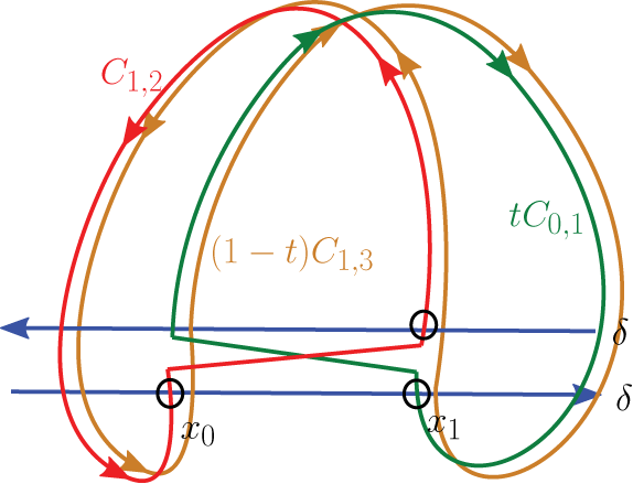
Figure 9.1 Example of a first iteration of the smeared first return map; that is,
 $[M^1]$
on a geodesic current corresponding to a closed curve intersecting the cross section
$[M^1]$
on a geodesic current corresponding to a closed curve intersecting the cross section
 $\tau $
twice at points
$\tau $
twice at points
 $\vec {x_0},\vec {x_1}$
and the cross section
$\vec {x_0},\vec {x_1}$
and the cross section
 $\tau _0$
once at point
$\tau _0$
once at point
 $\vec {x_1}$
. The weight of the bump function
$\vec {x_1}$
. The weight of the bump function
 $\psi $
at
$\psi $
at
 $\vec {x_0}$
is t. We obtain three weighted curves.
$\vec {x_0}$
is t. We obtain three weighted curves.
 $C_{0,1}$
consisting of the geodesic trajectory that goes from
$C_{0,1}$
consisting of the geodesic trajectory that goes from
 $\vec {x_0}$
to
$\vec {x_0}$
to
 $x_1$
and closes off by following the cross section in some coherent way.
$x_1$
and closes off by following the cross section in some coherent way.
 $C_{0,1}$
has weight 1 by definition of smeared return map, since
$C_{0,1}$
has weight 1 by definition of smeared return map, since
 $\vec {x_1} \in \tau _0$
.
$\vec {x_1} \in \tau _0$
.
 $C_{1,2}$
has weight t, whereas
$C_{1,2}$
has weight t, whereas
 $C_{1,3}$
has weight
$C_{1,3}$
has weight
 $1-t$
.
$1-t$
.
Now, the join lemma asserts that we can to join the curves
 $C_{0,1}$
and
$C_{0,1}$
and
 $C_{1,2}$
, together with an extra curve K, to get
$C_{1,2}$
, together with an extra curve K, to get
 $C_{0,2}$
. Assuming all of the relevant intersections are essential, we can do it with K being two copies of
$C_{0,2}$
. Assuming all of the relevant intersections are essential, we can do it with K being two copies of
 $\delta $
, one oriented in each direction, in the steps shown in Figure 9.2.
$\delta $
, one oriented in each direction, in the steps shown in Figure 9.2.

Figure 9.2 Applying the join lemma in Example 9.3. At each step, we smooth at the circled crossing.
In the full proof, to guarantee the analogous intersections are essential we will add more copies of
 $\delta $
.
$\delta $
.
Proof of Lemma 9.1. First we look at the geometry of a return trajectory
 $m^k(\vec {x})$
when k is large, as a concrete curve either on
$m^k(\vec {x})$
when k is large, as a concrete curve either on
 $\Sigma $
or lifted to the universal cover. Since there is a lower bound on the first return time (Lemma 7.3), the nth return time grows at least linearly in k. We may therefore assume that the portion of
$\Sigma $
or lifted to the universal cover. Since there is a lower bound on the first return time (Lemma 7.3), the nth return time grows at least linearly in k. We may therefore assume that the portion of
 $m^k(\vec {x})$
that follows
$m^k(\vec {x})$
that follows
 $\phi _t(\vec {x})$
is very long. The lift of
$\phi _t(\vec {x})$
is very long. The lift of
 $m^k(\vec {x})$
to the universal cover is thus a broken path: for some large L, it alternates between
$m^k(\vec {x})$
to the universal cover is thus a broken path: for some large L, it alternates between
-
(a) long segments of length at least L following
$\phi _t(\vec {x})$
and -
(b) short segments of some length following
$\delta $
,


with turns between them that are within
 $\varepsilon $
of a right angle, alternating left and right. (See Definition 12.1 for a precise definition.)
$\varepsilon $
of a right angle, alternating left and right. (See Definition 12.1 for a precise definition.)
We study the geometry of broken paths in Section 12. In particular, we prove several lemmas there guaranteeing that broken paths intersect essentially in certain circumstances. If L is large enough, we have the following results:
-
• A broken path and a lift of
$\delta $
intersect essentially (Lemma 12.2). -
• Broken paths with short segments that are different enough in length intersect essentially (Lemma 12.3).

We first prove part (a) in the lemma statement. We will use the following steps. By convention,
 $\delta $
is oriented to the right and
$\delta $
is oriented to the right and
 $\delta ^{-1}$
is the same curve oriented to the left. Let
$\delta ^{-1}$
is the same curve oriented to the left. Let
 $\alpha $
,
$\alpha $
,
 $\beta $
and
$\beta $
and
 $\gamma $
be
$\gamma $
be
 $m^k(\vec x)$
and
$m^k(\vec x)$
and
 $m^\ell (p^k(\vec x))$
, respectively.
$m^\ell (p^k(\vec x))$
, respectively.
-
(1) We start by smoothing
$[\alpha ]$
with a large number N of copies of
$[\delta ]$
. Each one of these intersections is essential by Lemma 12.2. This yields a new curve
$[\alpha _1]$
with lift a broken path with an lengthened short segment. -
(2) We then smooth
$[\alpha _1]$
against
$[\beta ]$
. The corresponding lifts are broken paths with short segments of different enough lengths, so Lemma 12.3 guarantees that the crossing is essential, yielding a new curve
$[\gamma _1]$
. -
(3) Finally, we smooth
$[\gamma _1]$
against
$N[\delta ^{-1}]$
. This returns to the correct homotopy class, again using Lemma 12.2 to guarantee that the crossings are essential. The result is
$[\gamma ]$
, as desired.


We need to use a large enough number N of copies of
 $\delta $
that guarantees that the crossing in the second step above is essential. Let
$\delta $
that guarantees that the crossing in the second step above is essential. Let
 $\varepsilon $
be the angle of the wedge set, let
$\varepsilon $
be the angle of the wedge set, let
 $\ell $
be the length of
$\ell $
be the length of
 $\delta $
and let
$\delta $
and let
 $\kappa (\varepsilon )$
be the constant from Lemma 12.3. Then we claim that it suffices to take
$\kappa (\varepsilon )$
be the constant from Lemma 12.3. Then we claim that it suffices to take
 $N = 2M$
with
$N = 2M$
with
 $M = 1+\lceil \kappa (\varepsilon )/\ell \rceil $
, so that overall constants in the statement are
$M = 1+\lceil \kappa (\varepsilon )/\ell \rceil $
, so that overall constants in the statement are
 $$ \begin{align*} K_\tau &= N\bigl([\delta] + [\delta^{-1}]\bigr)\\ w_\tau &= 2N+1 = 3 + 4\lceil\kappa(\varepsilon)/\ell\rceil. \end{align*} $$
In order to be explicit about how to apply Lemmas 12.2 and 12.3, we will work with concrete lifts of our curves to broken paths in the universal cover; to pick out a lift, we work with elements of
 $\pi _1$
and so pick a basepoint. For concreteness, choose the basepoint
$\pi _1$
and so pick a basepoint. For concreteness, choose the basepoint
 $*$
to be at the far left end of the segment on
$*$
to be at the far left end of the segment on
 $\delta $
defining
$\delta $
defining
 $\tau '$
. (Recall that we removed a short interval to make
$\tau '$
. (Recall that we removed a short interval to make
 $\tau '$
simply connected.) We are particularly interested in the short segments on the lift of
$\tau '$
simply connected.) We are particularly interested in the short segments on the lift of
 $\delta $
; for that purpose, parametrise the lift of
$\delta $
; for that purpose, parametrise the lift of
 $\delta $
by length in
$\delta $
by length in
 $\mathbb {R}$
, with
$\mathbb {R}$
, with
 $0$
at the lift of the basepoint
$0$
at the lift of the basepoint
 $*$
and
$*$
and
 $\delta $
oriented in the positive direction so that
$\delta $
oriented in the positive direction so that
 $\delta $
itself lifts to a curve ending at
$\delta $
itself lifts to a curve ending at
 $\ell $
.
$\ell $
.
Now we state precisely the sequence of smoothings that we will perform, illustrating them with slightly schematic figures of both the curves on the surface and of the corresponding broken paths realising the lifts in the universal cover. At each step we circle the crossings that we smooth at the next step.
-
(i) Let
$\delta , \alpha $
and
$\beta $
be elements of
$\pi _1(S)$
representing the transversal curve,
$m^k(\vec {x})$
and
$m^\ell (p^k(\vec {x}))$
, respectively:The endpoints of the central short segments of lifts of
$\alpha $
and
$\beta $
are both in
$(0,\ell )$
, in the parametrisation above. -
(ii) Smooth
$[\alpha ]$
with
$N[\delta ]$
a total of N times to get
$[\alpha _1]$
with
$\alpha _1 = \delta ^M\alpha \delta ^M$
. The crossings are essential by Lemma 12.2.The endpoints of the central short segment of the lift of
$\alpha _1$
are in
$(-M\ell ,-(M-1)\ell )$
and in
$(M\ell ,(M+1)\ell )$
. -
(iii) Smooth
$[\alpha \delta ^N] \cup [\beta ]$
at a middle crossing to make
$[\gamma _1] = [\alpha \delta ^{M} \beta \delta ^{M}]$
. Since
$(M-1)\ell \ge \kappa (\varepsilon )$
, the crossing is essential by Lemma 12.3.Here, in the picture in the universal cover, two different lifts of
$\gamma _1$
are shown (one dashed), to make it clearer what happened in the smoothing; these are the lifts of
$\delta ^{M} \alpha \delta ^{M} \beta $
(solid) and
$\beta \delta ^{M} \alpha \delta ^{M}$
(dashed). -
(iv) Smooth
$[\gamma _1]$
with
$N[\delta ^{-1}]$
a total of N times at appropriate crossings to make
$[\alpha \beta ] = m^{k+\ell }(\vec x)$
. The crossings are essential by Lemma 12.2. -
(v) The result is
$[\alpha \beta ]$
as desired.


This completes the proof of part (a) of the statement. Part (b) is very similar. Precisely, we do the following steps.
-
(i ′ ) Let
$\delta = \tau $
,
$\alpha = m^k(\vec x)$
and
$\beta = m^\ell (p^k(\vec x))$
be as before, so that we start with
$[\alpha \beta ] = [m^{k+\ell }(\vec x)]$
. -
(ii ′ ) Use Lemma 12.2 to smooth with
$N[\delta ]$
a total of N times to get
$[\gamma _1]$
with
$\gamma _1 = \delta ^M\alpha \beta \delta ^M$
. If we set
$\gamma _2 = \beta \delta ^N\alpha $
, then
$[\gamma _1] = [\gamma _2]$
, but these two curves have different canonical lifts to the universal cover: the endpoints of the primary short segment
$\gamma _1$
are in
$(-M\ell ,-(M-1)\ell )$
and
$(M\ell ,(M+1)\ell )$
on the lift of
$\delta $
, while the endpoints of the (zero-length) primary ‘short segment’ of
$\gamma _2$
are at the same point in
$(0,\ell )$
. -
(iii ′ ) Smooth
$[\gamma _1]$
with itself to make
$[\alpha _1] \cup [\beta _1]$
, with
$\alpha _1 = \delta ^M\alpha $
and
$\beta _1 = \beta \delta ^M$
. The crossing corresponds to the lifts given by
$\gamma _1$
and
$\gamma _2$
and is essential by Lemma 12.3. -
(iv ′ ) Smooth
$[\alpha _1]$
and
$[\beta _1]$
each M times with
$M[\delta ^{-1}]$
to make
$[\alpha ]$
and
$[\beta ]$
, respectively, using Lemma 12.2. -
(v ′ ) The result is
$[\alpha ] \cup [\beta ]$
as desired.


Proof of Lemma 9.2. By definition of
 $M^k$
and
$M^k$
and
 $P^k$
, we have nonnegative constants K,
$P^k$
, we have nonnegative constants K,
 $a_i$
, L and
$a_i$
, L and
 $b_{i,j}$
so that
$b_{i,j}$
so that
 $$ \begin{align*} M^k(\vec{x}) &= \sum_{i=k}^K a_i m^i(\vec{x}) & P^k(\vec{x}) &= \sum_{i=k}^K a_i \vec{y_i}\\ M^\ell(\vec{y_i}) &= \sum_{j=\ell}^L b_{i,j} m^j(\vec{y_i}) & M^{k+\ell}(\vec{x}) &= \sum_{i=k}^K \sum_{j=l}^L a_i b_{i,j} m^i(\vec{x}) m^j(\vec{y_i}). \end{align*} $$
Furthermore,
 $\sum _i a_i = 1$
and, for fixed i,
$\sum _i a_i = 1$
and, for fixed i,
 $\sum _j b_{i,j} = 1$
. The result follows by distributing and applying Lemma 9.1 repeatedly.
$\sum _j b_{i,j} = 1$
. The result follows by distributing and applying Lemma 9.1 repeatedly.
As an immediate consequence, we have the following.
Proposition 9.4. For a fixed good cross section
 $\tau $
as constructed above and for every curve functional f satisfying quasi-smoothing and convex union, there is a constant
$\tau $
as constructed above and for every curve functional f satisfying quasi-smoothing and convex union, there is a constant
 $\kappa (\tau )$
so that, for sufficiently large
$\kappa (\tau )$
so that, for sufficiently large
 $k,\ell $
and every geodesic current
$k,\ell $
and every geodesic current
 $\mu $
, we have
$\mu $
, we have
 $$ \begin{align*} f^{k+\ell}_{\tau}(\mu) \le f^k_{\tau}(\mu) + f^\ell_{\tau}(\mu) + \kappa(\tau)\mu(\psi\tau). \end{align*} $$
Proof. We will prove this with
 $\kappa (\tau ) = f(K_\tau ) + R w_\tau $
, where
$\kappa (\tau ) = f(K_\tau ) + R w_\tau $
, where
 $K_\tau $
and
$K_\tau $
and
 $w_\tau $
are from Lemma 9.2 and R is the quasi-smoothing constant from equation (1.2).
$w_\tau $
are from Lemma 9.2 and R is the quasi-smoothing constant from equation (1.2).
We have
 $$ \begin{align*} f^{k+\ell}_\tau(\mu) &= f\left(\int_\tau M^{k+\ell}(\vec{x}) \psi(\vec{x})\mu(\vec{x})\right)\\ &\le f\left(\int_\tau \bigl(M^k(\vec{x}) + M^\ell(P^k(\vec{x})) + K_\tau\bigr) \psi(x)\mu(x)\right) + \int_\tau R w_\tau \psi(\vec{x}) \mu(\vec{x})\\ &\le f\left(\int_\tau M^k(x)\psi(\vec{x})\mu(\vec{x})\right) + f\left(\int_\tau M^\ell(P^k(\vec{x}))\psi(\vec{x})\mu(\vec{x})\right) + \kappa(\tau)\int_\tau \psi(\vec{x})\mu(\vec{x})\\ &= f^k(\mu) + f\left(\int_\tau M^\ell(\vec{x})P^k_*(\psi(\vec{x})\mu(\vec{x}))\right) + \kappa(\tau)\mu(\psi\tau)\\ &= f^k(\mu) + f^\ell(\mu) + \kappa(\tau)\mu(\psi\tau), \end{align*} $$
where we use, successively:


We recall a slight variation of Fekete’s lemma, which follows from standard versions, such as de Bruijn and Erdös [Reference de Bruijn and Erdös17, Theorem 22].
Lemma 9.5 Fekete’s lemma
Let
 $(a_n)_{n=1}^\infty $
be a sequence of real numbers and suppose there exists N such that for all
$(a_n)_{n=1}^\infty $
be a sequence of real numbers and suppose there exists N such that for all
 $m,n \geq N$
,
$m,n \geq N$
,
 $a_{n+m} \le a_n + a_m$
. Then
$a_{n+m} \le a_n + a_m$
. Then
 $$ \begin{align*} \lim_{n \to \infty}\frac{a_n}{n} \quad\text{exists and is equal to}\quad \inf_{n\ge N} \frac{a_n}{n}. \end{align*} $$
Finally, we can show that the limit defining the extension of f exists.
Proposition 9.6. For any curve functional f satisfying quasi-smoothing and convex union, the limit defining
 $f_\tau $
in equation (7.27) exists.
$f_\tau $
in equation (7.27) exists.
10 Continuity of the extension
In order to prove continuity of the extension, we will prove continuity of
 $f^k_\tau $
and then get upper and lower bounds on the limit
$f^k_\tau $
and then get upper and lower bounds on the limit
 $f_\tau (\mu )$
in terms of
$f_\tau (\mu )$
in terms of
 $f^k_\tau (\mu )$
. Proposition 9.4 lets us use Fekete’s lemma to get upper bounds. To get lower bounds, we have the following.
$f^k_\tau (\mu )$
. Proposition 9.4 lets us use Fekete’s lemma to get upper bounds. To get lower bounds, we have the following.
Proposition 10.1. For a fixed good cross section
 $\tau $
and any weighted curve functional f satisfying homogeneity, weighted quasi-smoothing and convex union, there is a constant
$\tau $
and any weighted curve functional f satisfying homogeneity, weighted quasi-smoothing and convex union, there is a constant
 $K(\mu ) = \kappa (\tau )\mu (\psi \tau )$
so that for all sufficiently large k and every geodesic current
$K(\mu ) = \kappa (\tau )\mu (\psi \tau )$
so that for all sufficiently large k and every geodesic current
 $\mu $
we have
$\mu $
we have
 $$ \begin{align*} 2f^{k}_{\tau}(\mu) \leq f^{2k}_{\tau}(\mu) + K(\mu). \end{align*} $$
Proof. By Lemma 9.2(b) in the case
 $k=\ell $
,
$k=\ell $
,
 $$ \begin{align*} M^{2k}(\vec{x}) \cup K_\tau \mathrel{\searrow}_{w_\tau} M^k(\vec{x}) \cup M^k(P^k(\vec{x})). \end{align*} $$
Integrating this statement with respect to the measure
 $\psi \mu $
(which is invariant under
$\psi \mu $
(which is invariant under
 $P^k$
), we find that
$P^k$
), we find that
 $$ \begin{align*} M^{2k}(\psi\mu) \cup K_\tau\cdot \mu(\psi\tau) \mathrel{\searrow}_{w_\tau \mu(\psi\tau)} 2M^k(\psi\mu). \end{align*} $$
Applying f to both sides and using homogeneity of f gives the desired result.
Since f is not in general additive, by comparison to Proposition 9.4, Proposition 10.1 is more restrictive, requiring
 $k=\ell $
. This still suffices to show that the
$k=\ell $
. This still suffices to show that the
 $f^k_\tau $
approximate
$f^k_\tau $
approximate
 $f_\tau $
well.
$f_\tau $
well.
Lemma 10.2. Let
 $\tau $
be fixed good cross section and f be a weighted curve functional satisfying homogeneity, weighted quasi-smoothing and convex union. For any sufficiently large k,
$\tau $
be fixed good cross section and f be a weighted curve functional satisfying homogeneity, weighted quasi-smoothing and convex union. For any sufficiently large k,
 $$ \begin{align*} {\lvert} f_{\tau}(\mu)-\frac{f^{k}_{\tau}(\mu)}{k} {\rvert} \leq \frac{K(\mu)}{k} \end{align*} $$
where
 $K(\mu ) = \kappa (\tau )\mu (\psi \tau )$
is the constant from Propositions 9.4 and 10.1.
$K(\mu ) = \kappa (\tau )\mu (\psi \tau )$
is the constant from Propositions 9.4 and 10.1.
Proof. From Propositions 9.4 and 10.1, for large enough k we have
 $$ \begin{align*} \Bigl| \frac{f^{2k}_{\tau}(\mu)}{2k}-\frac{f^{k}_{\tau}(\mu)}{k}\Bigr| \leq \frac{K(\mu)}{2k}. \end{align*} $$
We also have
 $$ \begin{align*} \frac{f^{k}_{\tau}(\mu)}{k} + \Big(\frac{f^{2k}_{\tau}(\mu)}{2k} - \frac{f^{k}_{\tau}(\mu)}{k} \Big) + \Big(\frac{f^{4k}_{\tau}(\mu)}{4k} - \frac{f^{2k}_{\tau}(\mu)}{2k} \Big) &+ \Big(\frac{f^{8k}_{\tau}(\mu)}{8k} - \frac{f^{4k}_{\tau}(\mu)}{4k} \Big) + \cdots \\ &= \lim_{n \to \infty} \frac{f^{2^nk}_{\tau}(\mu)}{2^nk} = \lim_{n \to \infty} \frac{f^{nk}_{\tau}(\mu)}{nk} =f_{\tau}(\mu), \end{align*} $$
where the first equality follows by telescoping and the second one because we have already proved that the limit exists. We can then give bounds:
 $$ \begin{align*} {\lvert} f_{\tau}(\mu)-\frac{f^{k}_{\tau}(\mu)}{k} {\rvert} &\leq {\lvert} \frac{f^{2k}_{\tau}(\mu)}{2k} -\frac{f^{k}_{\tau}(\mu)}{k} {\rvert} + {\lvert} \frac{f^{4k}_{\tau}(\mu)}{4k} -\frac{f^{2k}_{\tau}(\mu)}{2k} {\rvert} + {\lvert} \frac{f^{8k}_{\tau}(\mu)}{8k} -\frac{f^{4k}_{\tau}(\mu)}{4k} {\rvert} + \cdots\\ &\leq \frac{K(\mu)}{2k} + \frac{K(\mu)}{4k} + \frac{K(\mu)}{8k} + \cdots \\ &= \frac{K(\mu)}{k}. \end{align*} $$
We next prove that the
 $f^k_\tau $
are continuous.
$f^k_\tau $
are continuous.
Proposition 10.3. Let
 $\tau $
be fixed good cross section and f be a weighted curve functional satisfying homogeneity, weighted quasi-smoothing and convex union. Then the functions
$\tau $
be fixed good cross section and f be a weighted curve functional satisfying homogeneity, weighted quasi-smoothing and convex union. Then the functions
 $f^{k}_{\tau }\colon \mathcal {GC}^+(S) \to \mathbb {R}$
are continuous for every k.
$f^{k}_{\tau }\colon \mathcal {GC}^+(S) \to \mathbb {R}$
are continuous for every k.
We will break the proof into lemmas.
Lemma 10.4. For
 $\tau $
a (closed) global cross section with interior
$\tau $
a (closed) global cross section with interior
 $\tau ^\circ $
, the map
$\tau ^\circ $
, the map
 $\mu \mapsto \mu _{\tau ^\circ }$
from
$\mu \mapsto \mu _{\tau ^\circ }$
from
 $\mathcal {GC}^+(S)$
to
$\mathcal {GC}^+(S)$
to
 $\mathcal {M}(\tau ^\circ )$
is continuous.
$\mathcal {M}(\tau ^\circ )$
is continuous.
Proof. We first adjust the definition of the flux
 $\mu _{\tau ^\circ }$
. Let
$\mu _{\tau ^\circ }$
. Let
 $\varepsilon $
be small enough so that the corresponding flow box is embedded. Pick a nonzero continuous function
$\varepsilon $
be small enough so that the corresponding flow box is embedded. Pick a nonzero continuous function
 $\omega \colon [0,\varepsilon ] \to \mathbb {R}_{\ge 0}$
so that
$\omega \colon [0,\varepsilon ] \to \mathbb {R}_{\ge 0}$
so that
 $\omega (0) = \omega (\varepsilon ) = 0$
and
$\omega (0) = \omega (\varepsilon ) = 0$
and
 $\int _0^\varepsilon \omega (t)\,dt = 1$
. Then, for any measurable function r on
$\int _0^\varepsilon \omega (t)\,dt = 1$
. Then, for any measurable function r on
 $\tau ^\circ $
, the flux
$\tau ^\circ $
, the flux
 $\mu _{\tau ^\circ }$
satisfies
$\mu _{\tau ^\circ }$
satisfies
 $$ \begin{align} \int_{\vec{x} \in \tau^\circ} r(\vec{x})\,\mu_{\tau^\circ}(\vec{x}) = \int_{t=0}^\varepsilon \int_{\vec{x} \in \tau^\circ} \omega(t) r(\vec{x})\,\mu\bigl(\phi_t(\vec{x})\bigr). \end{align} $$
Now suppose that we have a sequence of measures
 $\mu _i$
approaching
$\mu _i$
approaching
 $\mu $
in the weak
$\mu $
in the weak
 $^*$
topology, and let r be a continuous function on
$^*$
topology, and let r be a continuous function on
 $\tau ^\circ $
with compact support. By Theorem 2.19, it suffices to show that
$\tau ^\circ $
with compact support. By Theorem 2.19, it suffices to show that
 $\int _{\vec {x} \in \tau ^\circ } r(\vec {x}) \, \mu _{i,\tau ^\circ }(\vec {x})$
converges to
$\int _{\vec {x} \in \tau ^\circ } r(\vec {x}) \, \mu _{i,\tau ^\circ }(\vec {x})$
converges to
 $\int _{\vec {x}\in \tau ^\circ } r(\vec {x}) \,\mu _{\tau ^\circ }(\vec {x})$
.
$\int _{\vec {x}\in \tau ^\circ } r(\vec {x}) \,\mu _{\tau ^\circ }(\vec {x})$
.
Consider the function s on
 $UT\Sigma $
defined by
$UT\Sigma $
defined by
 $$ \begin{align*} s(\vec{x}) = \begin{cases} r(\vec{x})\omega(t) & \text{if}\ y = \phi_t(\vec{x})\ \text{for}\ \vec{x}\in\tau, t \in [0,\varepsilon]\\ 0 & \text{otherwise}. \end{cases} \end{align*} $$
Then s is continuous, since r and
 $\omega $
vanish on the boundaries of their domains of definition, so
$\omega $
vanish on the boundaries of their domains of definition, so
 $\int _{\vec {y} \in UT\Sigma } s(\vec x) \mu _i(\vec {y})$
converges to
$\int _{\vec {y} \in UT\Sigma } s(\vec x) \mu _i(\vec {y})$
converges to
 $\int _{\vec {y} \in UT\Sigma } s(\vec {y}) \mu (\vec {y})$
. The result follows from equation (10.5).
$\int _{\vec {y} \in UT\Sigma } s(\vec {y}) \mu (\vec {y})$
. The result follows from equation (10.5).
Remark 10.6. The map
 $\mu \mapsto \mu _\tau $
from
$\mu \mapsto \mu _\tau $
from
 $\mathcal {GC}^+(S)$
to positive measures
$\mathcal {GC}^+(S)$
to positive measures
 $\mathcal {M}(\tau )$
on the closed cross section is not continuous with respect to the weak
$\mathcal {M}(\tau )$
on the closed cross section is not continuous with respect to the weak
 $^*$
topology at points where
$^*$
topology at points where
 $\mu _\tau (\partial \tau ) \neq 0$
. Indeed, let
$\mu _\tau (\partial \tau ) \neq 0$
. Indeed, let
 $\mu $
be the geodesic current corresponding to a closed curve
$\mu $
be the geodesic current corresponding to a closed curve
 $[a]$
, let
$[a]$
, let
 $[b]$
be another closed curve intersecting
$[b]$
be another closed curve intersecting
 $[a]$
and let
$[a]$
and let
 $\mu _n$
be the geodesic current corresponding to
$\mu _n$
be the geodesic current corresponding to
 $\frac {1}{n} [a^nb]$
so that
$\frac {1}{n} [a^nb]$
so that
 $\lim _{n\to \infty } \mu _n = \mu $
, as shown in Figure 10.1. Take a (noncomplete) transversal
$\lim _{n\to \infty } \mu _n = \mu $
, as shown in Figure 10.1. Take a (noncomplete) transversal
 $\tau $
that intersects
$\tau $
that intersects
 $\operatorname {\mathrm {supp}}(\mu )$
only once on
$\operatorname {\mathrm {supp}}(\mu )$
only once on
 $\partial \tau $
. Then (for appropriate choices, as shown) the total mass of
$\partial \tau $
. Then (for appropriate choices, as shown) the total mass of
 $\mu _n$
– that is,
$\mu _n$
– that is,
 $(\mu _n)_\tau (\tau )$
– is approximately
$(\mu _n)_\tau (\tau )$
– is approximately
 $1/2$
, while
$1/2$
, while
 $\mu _\tau (\tau ) = 1$
.
$\mu _\tau (\tau ) = 1$
.

Figure 10.1 An example showing that the flux map
 $\mu \mapsto \mu _\tau $
is not continuous. The sequence of curves
$\mu \mapsto \mu _\tau $
is not continuous. The sequence of curves
 $[a^nb]/n$
approaches
$[a^nb]/n$
approaches
 $[a]$
, but they have very different intersections with
$[a]$
, but they have very different intersections with
 $\tau $
.
$\tau $
.
Similarly, for the open transversals
 $\tau ^\circ $
, we have
$\tau ^\circ $
, we have
 $\mu _{\tau ^\circ }(\tau ^\circ ) = 0$
while
$\mu _{\tau ^\circ }(\tau ^\circ ) = 0$
while
 $(\mu _n)_{\tau ^\circ }(\tau ^\circ )$
is approximately
$(\mu _n)_{\tau ^\circ }(\tau ^\circ )$
is approximately
 $1/2$
for large n. This does not contradict Lemma 10.4; it just says that total mass is not a continuous function in the weak
$1/2$
for large n. This does not contradict Lemma 10.4; it just says that total mass is not a continuous function in the weak
 $^*$
topology on a noncompact space.
$^*$
topology on a noncompact space.
Lemma 10.7. The extension of
 $[M^k]$
to measures, as a map from
$[M^k]$
to measures, as a map from
 $\mathcal {M}(\tau )$
to
$\mathcal {M}(\tau )$
to
 $\mathbb {R}\mathcal {C}(S)$
, is continuous.
$\mathbb {R}\mathcal {C}(S)$
, is continuous.
Proof. Recall from Lemma 7.23 that
 $[M^k(\mu )]$
takes values in the finite-dimensional subspace
$[M^k(\mu )]$
takes values in the finite-dimensional subspace
 $\mathbb {R}{[\Lambda (k,\tau ,\tau _0)]} \subset \mathbb {R}\mathcal {C}(S)$
. By continuity of
$\mathbb {R}{[\Lambda (k,\tau ,\tau _0)]} \subset \mathbb {R}\mathcal {C}(S)$
. By continuity of
 $[M^k(\vec {x})]$
(Lemma 7.24), we can write
$[M^k(\vec {x})]$
(Lemma 7.24), we can write
 $$ \begin{align*} [M^k(\vec{x})] = \sum_{C \in [\Lambda(k,\tau,\tau_0)]} a_C(\vec{x}) \cdot C \end{align*} $$
where
 $a_C$
is a continuous function on
$a_C$
is a continuous function on
 $\tau $
. (Recall that a function to a finite-dimensional vector space is continuous iff each of the coordinate functions is continuous; see Remark 2.25.) But then
$\tau $
. (Recall that a function to a finite-dimensional vector space is continuous iff each of the coordinate functions is continuous; see Remark 2.25.) But then
 $$ \begin{align*} [M^k(\mu)] = \sum_{C \in[\Lambda(k,\tau,\tau_0)]} \left(\int_{\vec{x} \in \tau} a_C(\vec{x})\,\mu(\vec{x})\right) \cdot C. \end{align*} $$
The integrals are continuous functions of
 $\mu $
by definition of the weak
$\mu $
by definition of the weak
 $^*$
topology on
$^*$
topology on
 $\mathcal {M}(\tau )$
.
$\mathcal {M}(\tau )$
.
Proof of Proposition 10.3.
 $f^k_\tau $
is the composition of maps
$f^k_\tau $
is the composition of maps
 $$ \begin{align*} \mathcal{GC}^+(S) \xrightarrow{\mu \mapsto \mu_{\tau^\circ}} \mathcal{M}(\tau^\circ) \xrightarrow{\cdot \psi} \mathcal{M}(\tau) \xrightarrow{[M^k]} \mathbb{R}^{\Lambda(k,\tau,\tau_0)} \overset{f}{\longrightarrow} \mathbb{R}. \end{align*} $$
The component maps are continuous by, respectively, Lemma 10.4, the fact that
 $\psi $
vanishes on a neighbourhood of
$\psi $
vanishes on a neighbourhood of
 $\partial \tau $
, Lemma 10.7 and Proposition 3.4.
$\partial \tau $
, Lemma 10.7 and Proposition 3.4.
Proposition 10.8. Let
 $\tau $
be fixed good cross section and f be a curve functional satisfying homogeneity, weighted quasi-smoothing and convex union. Then
$\tau $
be fixed good cross section and f be a curve functional satisfying homogeneity, weighted quasi-smoothing and convex union. Then
 $f_{\tau }\colon \mathcal {GC}^+(S) \to \mathbb {R}_{ \geq 0}$
is a continuous function.
$f_{\tau }\colon \mathcal {GC}^+(S) \to \mathbb {R}_{ \geq 0}$
is a continuous function.
Proof. By Proposition 10.3, it suffices to show that
 $f_\tau $
is a uniform limit of
$f_\tau $
is a uniform limit of
 $f^k_\tau $
. The constant
$f^k_\tau $
. The constant
 $K(\mu )$
in Lemma 10.2 does depend on
$K(\mu )$
in Lemma 10.2 does depend on
 $\mu $
; however, if we bound
$\mu $
; however, if we bound
 $\mu $
within a ball so that
$\mu $
within a ball so that
 $\int _\tau \psi \mu _\tau $
is bounded, the constant in the approximation becomes uniform and tends to
$\int _\tau \psi \mu _\tau $
is bounded, the constant in the approximation becomes uniform and tends to
 $0$
as
$0$
as
 $k \to \infty $
.
$k \to \infty $
.
11 The extension extends
In this section we prove that when restricted to weighted curves, the purported extension
 $f_{\tau }$
coincides with the original curve functional f. More precisely, let
$f_{\tau }$
coincides with the original curve functional f. More precisely, let
 $\gamma \in C$
be the geodesic representative of an oriented closed curve with corresponding geodesic current
$\gamma \in C$
be the geodesic representative of an oriented closed curve with corresponding geodesic current
 $\mu _C$
, and let
$\mu _C$
, and let
 $\tau $
be a good cross section of the geodesic flow (Definition 8.4). We wish to show that
$\tau $
be a good cross section of the geodesic flow (Definition 8.4). We wish to show that
 $f_\tau (\mu _C) = f(C)$
.
$f_\tau (\mu _C) = f(C)$
.
Let
 $\widetilde {\gamma }$
be the canonical lift of
$\widetilde {\gamma }$
be the canonical lift of
 $\gamma $
to the unit tangent bundle, and let n be the number of times that
$\gamma $
to the unit tangent bundle, and let n be the number of times that
 $\widetilde {\gamma }$
intersects
$\widetilde {\gamma }$
intersects
 $\tau $
, with intersections at
$\tau $
, with intersections at
 $\vec x_0, \vec x_1,\dots , \vec x_{n-1}$
in order (so
$\vec x_0, \vec x_1,\dots , \vec x_{n-1}$
in order (so
 $p(\vec x_i)=\vec x_{i+1}$
). Then
$p(\vec x_i)=\vec x_{i+1}$
). Then
 $(\mu _C)_{\tau }=\sum _{i=0}^{n-1} \vec x_i$
. Let
$(\mu _C)_{\tau }=\sum _{i=0}^{n-1} \vec x_i$
. Let
 $a_i=\psi (\vec x_i)$
, so that
$a_i=\psi (\vec x_i)$
, so that
 $$ \begin{align*} C \cap \psi\tau := \psi \cdot (\mu_C)_\tau = \sum_{i=0}^{n-1} a_i \vec x_i. \end{align*} $$
By Proposition 7.16, this sum (which we call
 $C \cap \psi \tau $
, in an abuse of notation) is invariant under the smeared return map P:
$C \cap \psi \tau $
, in an abuse of notation) is invariant under the smeared return map P:
 $$ \begin{align} P^k \biggl( \sum_{i=0}^{n-1} a_i \vec x_i \biggr)= \sum_{i=0}^{n-1} a_i \vec x_i. \end{align} $$
We need a slightly stronger fact. Recall that each term in
 $[M^k(C \cap \psi \tau )]$
is a curve that follows the geodesic trajectory
$[M^k(C \cap \psi \tau )]$
is a curve that follows the geodesic trajectory
 $\vec x_i \to \vec x_{i+1} \to \dots $
for some time and then travels along
$\vec x_i \to \vec x_{i+1} \to \dots $
for some time and then travels along
 $\tau $
to close up. We say that a segment of the return map
$\tau $
to close up. We say that a segment of the return map
 $\vec x_i \to \vec x_{i+1}$
is covered with degree r in
$\vec x_i \to \vec x_{i+1}$
is covered with degree r in
 $[M^k]$
if the weighted number of times that segment appears in
$[M^k]$
if the weighted number of times that segment appears in
 $[M^k(C \cap \psi \tau )]$
is r.
$[M^k(C \cap \psi \tau )]$
is r.
Lemma 11.2. For any closed curve C and a good cross section
 $\tau $
with bump function
$\tau $
with bump function
 $\psi $
as above, in
$\psi $
as above, in
 $[M^k(C \cap \psi \tau )]$
, every segment
$[M^k(C \cap \psi \tau )]$
, every segment
 $\vec x_{i} \to \vec x_{i+1}$
is covered with degree k.
$\vec x_{i} \to \vec x_{i+1}$
is covered with degree k.
(See Example 9.3 for one concrete case.)
Proof. Fix
 $a_i = \psi (\vec x_i)$
as above and consider the case
$a_i = \psi (\vec x_i)$
as above and consider the case
 $k=1$
. By the assumption that
$k=1$
. By the assumption that
 $\tau _0$
is a complete cross section, we have
$\tau _0$
is a complete cross section, we have
 $a_i=1$
for some i. By rotating the indices, assume
$a_i=1$
for some i. By rotating the indices, assume
 $a_0=1$
. We prove the statement for each segment
$a_0=1$
. We prove the statement for each segment
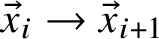 $\vec x_{i} \to \vec x_{i+1}$
by induction on i. For
$\vec x_{i} \to \vec x_{i+1}$
by induction on i. For
 $i=0$
, it is clear, since
$i=0$
, it is clear, since
 $a_0=1$
and no earlier trajectories continue through
$a_0=1$
and no earlier trajectories continue through
 $\vec x_0$
. For
$\vec x_0$
. For
 $i>0$
, we have
$i>0$
, we have
 $a_i$
trajectories starting at
$a_i$
trajectories starting at
 $\vec x_i$
and going to
$\vec x_i$
and going to
 $\vec x_{i+1}$
. By the induction hypothesis, we also have weight 1 of trajectories arriving at
$\vec x_{i+1}$
. By the induction hypothesis, we also have weight 1 of trajectories arriving at
 $\vec x_i$
from
$\vec x_i$
from
 $\vec x_{i-1}$
and so a weight of
$\vec x_{i-1}$
and so a weight of
 $1-a_i$
for those continuing on to
$1-a_i$
for those continuing on to
 $\vec x_{i+1}$
. These two types of trajectories have a total weight of
$\vec x_{i+1}$
. These two types of trajectories have a total weight of
 $1$
, as desired.
$1$
, as desired.
The statement for
 $k>1$
follows from equation (11.1) and induction.
$k>1$
follows from equation (11.1) and induction.
Now, for
 $i < j$
, let
$i < j$
, let
 $C_{ij}$
be the curve that starts at
$C_{ij}$
be the curve that starts at
 $\vec x_i$
, passes through
$\vec x_i$
, passes through
 $j-i-1$
intermediate points to
$j-i-1$
intermediate points to
 $\vec x_j$
and closes up along
$\vec x_j$
and closes up along
 $\tau $
, with indices interpreted modulo n. Then, for some coefficients
$\tau $
, with indices interpreted modulo n. Then, for some coefficients
 $w_{ij}$
, we can write
$w_{ij}$
, we can write
 $$ \begin{align*} \Bigl[M^k\Bigl(\sum a_i \vec x_i\Bigr)\Bigr] = \sum w_{ij} C_{ij}. \end{align*} $$
The nonzero coefficients
 $w_{ij}$
that appear will have
$w_{ij}$
that appear will have
 $k \le j - i \le kn$
, so as k gets large the
$k \le j - i \le kn$
, so as k gets large the
 $C_{ij}$
that appear in the weighted sum also get long.
$C_{ij}$
that appear in the weighted sum also get long.
The invariance from equation (11.1) tells us that for all
 $i_0$
,
$i_0$
,
 $$ \begin{align} \sum_{i \equiv i_0} w_{ij} = \sum_{j \equiv i_0} w_{ij} = a_{i_0} \end{align} $$
while the fact that all n steps
 $x_i \to x_{i+1}$
are covered with degree k implies that
$x_i \to x_{i+1}$
are covered with degree k implies that
 $$ \begin{align} \sum_{i,j} w_{ij} = kn. \end{align} $$
Proposition 11.5. If
 $\mu _C$
is the geodesic current associated to a weighted closed multi-curve C and
$\mu _C$
is the geodesic current associated to a weighted closed multi-curve C and
 $\tau $
is a good cross section of the geodesic flow, then
$\tau $
is a good cross section of the geodesic flow, then
 $f_{\tau }(\mu _C)=f(C)$
.
$f_{\tau }(\mu _C)=f(C)$
.
Proof. We first suppose C is a single curve with weight
 $1$
.
$1$
.
As above, let
 $\sum _{i=0}^{n-1} a_i \vec x_i = C \cap \psi \tau $
. For the kth iterate set
$\sum _{i=0}^{n-1} a_i \vec x_i = C \cap \psi \tau $
. For the kth iterate set
 $$ \begin{align*} C_0^k = \Bigl[M^k\Bigl(\sum a_i \vec x_i\Bigr)\Bigr]=\sum_{i<j} w_{ij}C_{ij}. \end{align*} $$
Note that
 $C_{i,i+rn} = C^r$
; other
$C_{i,i+rn} = C^r$
; other
 $C_{ij}$
have a more complicated relation to C. For k sufficiently large, we will use Lemma 9.2 to simplify the sum so that only curves of the form
$C_{ij}$
have a more complicated relation to C. For k sufficiently large, we will use Lemma 9.2 to simplify the sum so that only curves of the form
 $C_{i,i+rn}$
appear.
$C_{i,i+rn}$
appear.
For each
 $i=0,\dots ,n-1$
(in any order), consider all of the curves that either start or end at
$i=0,\dots ,n-1$
(in any order), consider all of the curves that either start or end at
 $\vec x_i$
, starting with
$\vec x_i$
, starting with
 $i = i_0$
. By equation (11.3),
$i = i_0$
. By equation (11.3),
 $$ \begin{align*} \sum_{\substack{i \equiv i_0\\j \not\equiv i_0}} w_{ij} = \sum_{\substack{i \not\equiv i_0\\j \equiv i_0}} w_{ij} \le a_{i_0}. \end{align*} $$
We can therefore pair the corresponding components of
 $C_0^k$
against each other using Lemma 9.2 pairwise in any order, getting a reduction
$C_0^k$
against each other using Lemma 9.2 pairwise in any order, getting a reduction
 $$ \begin{align*} C_0^k \cup a_{i_0} K \mathrel{\searrow}_{a_{i_0}w} C_1^k \end{align*} $$
where K and w are the curve and weight from Lemma 9.2, and
 $C_1^k$
is another weighted combination of the
$C_1^k$
is another weighted combination of the
 $C_{ij}$
in which each component that starts at
$C_{ij}$
in which each component that starts at
 $i_0$
also ends at
$i_0$
also ends at
 $i_0$
.
$i_0$
.
This join operation does not change the degree by which segments of the curves are covered, so equation (11.4) still holds, and equation (11.3) still holds at the other indices. So we can repeat this at each index. In the end we get a reduction
 $$ \begin{align*} C_0^k \cup aK \mathrel{\searrow}_{aw} \sum_j b_j C^j =: C_n^k \end{align*} $$
where
 $a = \sum _i a_i$
and
$a = \sum _i a_i$
and
 $C_n^k $
is another weighted curve. By considering the degrees, we see that
$C_n^k $
is another weighted curve. By considering the degrees, we see that
 $\sum jb_j = k$
.
$\sum jb_j = k$
.
Similar considerations (similar to part (b) of Lemma 9.2) show that
 $$ \begin{align*} C_n^k \cup aK \mathrel{\searrow}_{aw} C_0^k. \end{align*} $$
By Corollary 13.5, f satisfies strong stability. The homogeneity and strong stability properties then yield
 $$ \begin{align*} kf(C)=f(kC) = f\Bigl(\sum_j b_{j} j C\Bigr) = f\bigl(C_n^k\bigr). \end{align*} $$
Therefore, since
 $aK$
and
$aK$
and
 $aw$
are independent of k,
$aw$
are independent of k,
 $$ \begin{align*} f_{\tau}(\mu) = \lim_{k \to \infty} \frac{f(C_0^k)}{k} = \lim_{k \to \infty} \frac{f(C_n^k)}{k} = \lim_{k \to \infty} \frac{f(kC)}{k} = f(C). \end{align*} $$
We have thus proved that
 $f_{\tau }$
extends f on unweighted curves.
$f_{\tau }$
extends f on unweighted curves.
For the case of a general weighted curve
 $C = \sum w_\ell C_\ell $
, the proof proceeds as above, except that we start with the weighted intersection of C with the smeared cross section. More precisely, let
$C = \sum w_\ell C_\ell $
, the proof proceeds as above, except that we start with the weighted intersection of C with the smeared cross section. More precisely, let
 $\vec x_{\ell ,i}$
be the intersections of
$\vec x_{\ell ,i}$
be the intersections of
 $C_\ell $
with
$C_\ell $
with
 $\tau $
; then we work with
$\tau $
; then we work with
 $\sum _{\ell ,i} w_\ell \psi (x_{\ell ,i}) \cdot \vec x_{\ell ,i}$
, in the same way as above.
$\sum _{\ell ,i} w_\ell \psi (x_{\ell ,i}) \cdot \vec x_{\ell ,i}$
, in the same way as above.
12 Hyperbolic geometry estimates
We complete the proof of Theorem A by proving facts about the geometry of broken paths, as used in Section 9.
Definition 12.1. Fix a real length L and angle
 $\varepsilon < \pi /2$
. A broken path
$\varepsilon < \pi /2$
. A broken path
 $b(L,\varepsilon )$
is a concatenation of geodesic segments in
$b(L,\varepsilon )$
is a concatenation of geodesic segments in
 $\mathbb {H}^2$
that alternate between ‘long’ segments of length at least
$\mathbb {H}^2$
that alternate between ‘long’ segments of length at least
 $\ell $
and ‘short’ segments of unconstrained length, so that the angle between the long and short segments is within
$\ell $
and ‘short’ segments of unconstrained length, so that the angle between the long and short segments is within
 $\varepsilon $
of
$\varepsilon $
of
 $\pi /2$
, alternately turning left and right. See Figure 12.1 for an example. We will denote by
$\pi /2$
, alternately turning left and right. See Figure 12.1 for an example. We will denote by
 $a_i$
the hyperbolic line containing the ith short segment.
$a_i$
the hyperbolic line containing the ith short segment.

Figure 12.1 A broken path in the disk model. Here
 ${\lvert } \pi /2-\theta {\rvert } < \varepsilon $
.
${\lvert } \pi /2-\theta {\rvert } < \varepsilon $
.
We prove some basic facts about when broken paths cross.
Lemma 12.2. For any
 $0 < \varepsilon < \pi /2$
, there is a constant
$0 < \varepsilon < \pi /2$
, there is a constant
 $L_0(\varepsilon )$
so that, for any
$L_0(\varepsilon )$
so that, for any
 $L> L_0(\varepsilon )$
, any broken path
$L> L_0(\varepsilon )$
, any broken path
 $b(L,\varepsilon )$
converges to unique points at infinity that are on opposite sides of the hyperbolic line containing any short segment. As
$b(L,\varepsilon )$
converges to unique points at infinity that are on opposite sides of the hyperbolic line containing any short segment. As
 $\varepsilon $
approaches
$\varepsilon $
approaches
 $0$
, the constant
$0$
, the constant
 $L_0(\varepsilon )$
approaches
$L_0(\varepsilon )$
approaches
 $0$
as well.
$0$
as well.
That is, in Figure 12.1, the broken path crosses the dashed paths.
Proof. In fact, this is true as long as
 $L_0(\varepsilon )> 2\operatorname {\mathrm {gd}}^{-1}(\varepsilon )$
, where
$L_0(\varepsilon )> 2\operatorname {\mathrm {gd}}^{-1}(\varepsilon )$
, where
 $\operatorname {\mathrm {gd}}$
is the Gudermann function, defined, for instance, by
$\operatorname {\mathrm {gd}}$
is the Gudermann function, defined, for instance, by
 $\operatorname {\mathrm {gd}}(x) = \tan ^{-1}(\sinh (x))$
.
$\operatorname {\mathrm {gd}}(x) = \tan ^{-1}(\sinh (x))$
.
Let b be the broken path, and let
 $a_i$
be the hyperbolic line containing the ith short segment. Since the turns in b alternate to the left and to the right, b locally crosses each
$a_i$
be the hyperbolic line containing the ith short segment. Since the turns in b alternate to the left and to the right, b locally crosses each
 $a_i$
.
$a_i$
.
The bound on
 $L_0(\varepsilon )$
was chosen so that
$L_0(\varepsilon )$
was chosen so that
 $a_i$
and
$a_i$
and
 $a_{i+1}$
do not cross or meet at infinity. (Another way to say this is that
$a_{i+1}$
do not cross or meet at infinity. (Another way to say this is that
 $\pi /2 - \varepsilon $
is bigger than the angle of parallelism of
$\pi /2 - \varepsilon $
is bigger than the angle of parallelism of
 $L_0(\varepsilon )/2$
.) Thus, the path b crosses the sequence of noncrossing segments
$L_0(\varepsilon )/2$
.) Thus, the path b crosses the sequence of noncrossing segments
 $a_i$
and thus cannot cross a single
$a_i$
and thus cannot cross a single
 $a_i$
more than once, as desired.
$a_i$
more than once, as desired.
The fact that
 $L_0(\varepsilon )$
is strictly greater than
$L_0(\varepsilon )$
is strictly greater than
 $2\operatorname {\mathrm {gd}}^{-1}(\varepsilon )$
means that as
$2\operatorname {\mathrm {gd}}^{-1}(\varepsilon )$
means that as
 $i \to \pm \infty $
the endpoints of the segments
$i \to \pm \infty $
the endpoints of the segments
 $a_i$
get closer by a definite factor on
$a_i$
get closer by a definite factor on
 $\partial \mathbb {H}^2$
. Thus, in either direction, b converges to a definite point on the circle at infinity.
$\partial \mathbb {H}^2$
. Thus, in either direction, b converges to a definite point on the circle at infinity.
From now on, we assume that all broken paths have
 $L>L_0(\varepsilon )$
.
$L>L_0(\varepsilon )$
.
Lemma 12.3. Fix
 $0 < \varepsilon < \pi /2$
and
$0 < \varepsilon < \pi /2$
and
 $L> L_0(\varepsilon )$
. Then there is a constant
$L> L_0(\varepsilon )$
. Then there is a constant
 $\kappa (\varepsilon )$
with the following property. If
$\kappa (\varepsilon )$
with the following property. If
 $\gamma = b(L,\varepsilon )$
and
$\gamma = b(L,\varepsilon )$
and
 $\gamma ' = b'(L,\varepsilon )$
are two broken paths with a pair of short segments
$\gamma ' = b'(L,\varepsilon )$
are two broken paths with a pair of short segments
 $s_0 \subset s_0'$
on the same line
$s_0 \subset s_0'$
on the same line
 $a_0$
and
$a_0$
and
 $s_0'$
extends at least
$s_0'$
extends at least
 $\kappa (\varepsilon )$
farther along
$\kappa (\varepsilon )$
farther along
 $a_0$
in each direction than
$a_0$
in each direction than
 $s_0$
, then
$s_0$
, then
 $\gamma $
and
$\gamma $
and
 $\gamma '$
cross essentially on
$\gamma '$
cross essentially on
 $a_0$
.
$a_0$
.
Note that in the last claim there is no control on
 $\kappa (\varepsilon )$
.
$\kappa (\varepsilon )$
.
Proof. It is most convenient to work in the band model of the hyperbolic plane as in Figure 12.2. Focus first on the path
 $\gamma $
, and let
$\gamma $
, and let
 $s_0$
,
$s_0$
,
 $l_1$
and
$l_1$
and
 $s_1$
be the next short and long segments of
$s_1$
be the next short and long segments of
 $\gamma $
, and let
$\gamma $
, and let
 $a_1$
be the line containing
$a_1$
be the line containing
 $s_1$
. The line
$s_1$
. The line
 $a_1$
defines an interval on
$a_1$
defines an interval on
 $\partial \mathbb {H}^2$
that, by Lemma 12.2, must contain the endpoint of
$\partial \mathbb {H}^2$
that, by Lemma 12.2, must contain the endpoint of
 $\gamma $
. Now fix the endpoints of
$\gamma $
. Now fix the endpoints of
 $s_0$
and vary the other parameters defining the interval of
$s_0$
and vary the other parameters defining the interval of
 $a_1$
, namely,
$a_1$
, namely,
-
• the angles between
$s_0$
and
$l_1$
and between
$l_1$
and
$s_1$
, both in
$[\pi /2-\varepsilon ,\pi /2+\varepsilon ]$
, and -
• the length of
$l_1$
, in
$[L_0(\varepsilon ),\infty ]$
.


(If we allow
 $\ell _1$
to have infinite length, the interval degenerates to a single point on
$\ell _1$
to have infinite length, the interval degenerates to a single point on
 $\partial \mathbb {H}^2$
.) As the parameters vary, the interval varies continuously on
$\partial \mathbb {H}^2$
.) As the parameters vary, the interval varies continuously on
 $\partial \mathbb {H}^2$
, remaining disjoint from the endpoints of
$\partial \mathbb {H}^2$
, remaining disjoint from the endpoints of
 $a_0$
. By compactness of the domain, the union of these intervals is a larger interval
$a_0$
. By compactness of the domain, the union of these intervals is a larger interval
 $W \subset \partial \mathbb {H}^2$
that necessarily contains the endpoint of
$W \subset \partial \mathbb {H}^2$
that necessarily contains the endpoint of
 $\gamma $
for fixed endpoint of
$\gamma $
for fixed endpoint of
 $s_0$
. Figure 12.3 shows the presumably extremal possibilities for W in one example, but we do not need to identify the precise values.
$s_0$
. Figure 12.3 shows the presumably extremal possibilities for W in one example, but we do not need to identify the precise values.

Figure 12.2 Crossing broken paths in the bands model for Lemma 12.3 and its proof, showing the case when the windows nearly touch.

Figure 12.3 The window of possible endpoints of a broken path. The marked points are bounds on ends of broken paths
 $b(L,\varepsilon )$
with
$b(L,\varepsilon )$
with
 $L \ge L_0$
.
$L \ge L_0$
.
A similar argument applies to the endpoint of
 $\gamma '$
on the same side of
$\gamma '$
on the same side of
 $a_0$
: it must lie in another window
$a_0$
: it must lie in another window
 $W'$
on
$W'$
on
 $\partial \mathbb {H}^2$
. By symmetry, in the band model
$\partial \mathbb {H}^2$
. By symmetry, in the band model
 $W'$
is a translation of W by a (Euclidean) amount proportional to
$W'$
is a translation of W by a (Euclidean) amount proportional to
 $\kappa (\varepsilon )$
. Thus, for
$\kappa (\varepsilon )$
. Thus, for
 $\kappa (\varepsilon )$
sufficiently large, W and
$\kappa (\varepsilon )$
sufficiently large, W and
 $W'$
will be disjoint; one extremal case is shown in Figure 12.2.
$W'$
will be disjoint; one extremal case is shown in Figure 12.2.
Similar arguments apply to the other endpoints of
 $\gamma $
and
$\gamma $
and
 $\gamma '$
, implying that for large enough
$\gamma '$
, implying that for large enough
 $\kappa (\varepsilon )$
the paths cross essentially.
$\kappa (\varepsilon )$
the paths cross essentially.
13 Stable functions
Some curve functionals satisfy quasi-smoothing and convex union but are not stable or homogeneous on the nose. For example, the length of a curve with respect to an arbitrary generating set is of this form (Example 4.10). We fix this by passing to a stable length as in Theorem B. Recall that the stable curve functional
 ${\lVert } f {\rVert }$
is defined by
${\lVert } f {\rVert }$
is defined by
 $$ \begin{align*} {\lVert} f {\rVert}(C) := \lim_{n \to \infty} \frac{f(C^n)}{n}. \end{align*} $$
As in the proof of Theorem 6.1, we will consider weighted curve functionals. In this section we will prove the following theorem.
Theorem 13.1. Let f be a weighted curve functional satisfying weighted quasi-smoothing and convex union. Then the stabilised curve functional
 $$ \begin{align*} \|f\|(C) := \lim_{n \to \infty} \frac{f(C^n)}{n} \end{align*} $$
satisfies weighted quasi-smoothing, convex union, strong stability and homogeneity and thus extends to a continuous function on
 $\mathcal {GC}^+(S)$
.
$\mathcal {GC}^+(S)$
.
We first prove some lemmas.
Lemma 13.2. For any connected curve C and any sufficiently large
 $n,m \geq 0$
, there exists some curve K and weight w so that
$n,m \geq 0$
, there exists some curve K and weight w so that
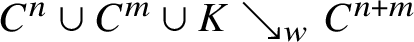 $C^n \cup C^m \cup K \mathrel {\searrow }_w C^{n+m}$
.
$C^n \cup C^m \cup K \mathrel {\searrow }_w C^{n+m}$
.
Proof. Let p be the number of intersections of our cross section
 $\tau $
with the canonical lift of C to
$\tau $
with the canonical lift of C to
 $UT\Sigma $
and apply Lemma 9.1(b), taking
$UT\Sigma $
and apply Lemma 9.1(b), taking
 $k=np$
and
$k=np$
and
 $l=mp$
. (We reuse the same cross section
$l=mp$
. (We reuse the same cross section
 $\tau $
for convenience; nothing here depends on the definition of the extension.) Then for sufficiently large
$\tau $
for convenience; nothing here depends on the definition of the extension.) Then for sufficiently large
 $n,m$
,
$n,m$
,
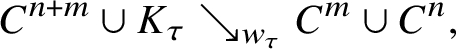 $$ \begin{align*} C^{n+m} \cup K_{\tau} &\mathrel{\searrow}_{w_\tau} C^m \cup C^n, \end{align*} $$
proving the lemma with
 $K = K_\tau $
and
$K = K_\tau $
and
 $w = w_\tau $
.
$w = w_\tau $
.
Lemma 13.3. For any connected curve C, we have
 $C^{n} \mathrel {\searrow }_{n-1} n C$
.
$C^{n} \mathrel {\searrow }_{n-1} n C$
.
Proof. Self-crossings of an n-fold cover of a curve are essential by definition.
Lemma 13.4. There is a curve K and a constant w so that, for any curve C on S and any
 $n \ge 2$
, we have
$n \ge 2$
, we have
 $$ \begin{align*} nC \cup (n-1)K\mathrel{\searrow}_{(n-1)w} C^n. \end{align*} $$
Proof. Pick
 $0 < \varepsilon < \pi /2$
so that
$0 < \varepsilon < \pi /2$
so that
 $L_0(\varepsilon )$
from Lemma 12.2 is less than the systole of
$L_0(\varepsilon )$
from Lemma 12.2 is less than the systole of
 $\Sigma $
, the length of the shortest closed geodesic on
$\Sigma $
, the length of the shortest closed geodesic on
 $\Sigma $
. As in Section 8, find a curve K and a complete global cross section
$\Sigma $
. As in Section 8, find a curve K and a complete global cross section
 $\tau \subset W(K, \varepsilon )$
. Then, by the arguments of Lemma 9.1(a), there is some integer w so that
$\tau \subset W(K, \varepsilon )$
. Then, by the arguments of Lemma 9.1(a), there is some integer w so that
 $$ \begin{align*} 2C \cup K \mathrel{\searrow}_{w} C^2. \end{align*} $$
(We are not directly applying Lemma 9.1, since we do not let the iteration in the return map go to infinity, but all of the long segments of the broken paths are long enough to make the arguments there work.) Iterating in this way, we deduce the desired result.
Proof of Theorem 13.1. We must show that
 ${\lVert } f {\rVert }$
is well-defined and satisfies convex union, weighted quasi-smoothing, strong stability and homogeneity. Let
${\lVert } f {\rVert }$
is well-defined and satisfies convex union, weighted quasi-smoothing, strong stability and homogeneity. Let
 $R\ge 0$
be the quasi-smoothing constant of f, and let K and w be the curves and constants from Lemmas 13.2 and 13.4 (which we can take to be the same), and let
$R\ge 0$
be the quasi-smoothing constant of f, and let K and w be the curves and constants from Lemmas 13.2 and 13.4 (which we can take to be the same), and let
 $f(K)^+$
be
$f(K)^+$
be
 $\max (f(K), 0)$
.
$\max (f(K), 0)$
.
-
• Well-defined: Lemma 13.2 shows that the sequence
$(f(C^n) + wR + f(K)^+)_{n \in \mathbb {N}}$
is subadditive for large enough n, and thus by Lemma 9.5 the limit defining
${\lVert } f {\rVert }$
exists. -
• Convex union: This follows immediately from the fact that
$(C_1 \cup C_2)^k = C_1^k \cup C_2^k$
, the definition of
${\lVert } f {\rVert }$
and convex union property of f. -
• Strong stability: For any multi-curve D and any curve C, by Lemmas 13.4 and 13.3 (applied to
$C^k)$
and the quasi-smoothing and convex union properties of f, we haveCombining the inequalities, dividing by k and letting k go to infinity, we obtain
$$ \begin{align*} f(D^k \cup C^{nk})-(n-1)wR &\leq f(D^k \cup nC^k) + (n-1)f(K)^+\\ f(D^k \cup nC^k)-(n-1)R &\leq f(D^k \cup C^{nk}). \end{align*} $$
We can iterate this to prove the result when C is a multi-curve.
$$ \begin{align*} {\lVert} f {\rVert}(D \cup C^n)&={\lVert} f {\rVert}(D \cup nC). \end{align*} $$
-
• Homogeneity: It is clear from the definition of
${\lVert } f {\rVert }$
that
${\lVert } f {\rVert }(C^n) = n{\lVert } f {\rVert }(C)$
. Homogeneity then follows from stability. -
• Weighted Quasi-smoothing: Let
$C = C_1 \cup C_2$
be a multi-curve, where the smoothing involves the component(s) in
$C_1$
, so that
$C_1$
and its smoothing
$C_1'$
each have at most two components. Thus,
$C_1^k \mathrel {\searrow }_{2(k-1)} k C_1$
and
$kC_1 \mathrel {\searrow }_k kC_1'$
. Thenso
$$ \begin{align*} {\lVert} f {\rVert}(C) &=\lim_{k \to \infty} \frac{f(C_1^k \cup C_2^k)}{k} \\ & \ge \lim_{k \to \infty} \frac{f(kC_1 \cup C_2^k)-2kR}{k} && \text{(Lemma~13.3)}\\ & \ge \lim_{k \to \infty} \frac{f(kC_1' \cup C_2^k) - 3kR}{k} && \text{(quasi-smoothing for}\ f\text{)}\\ &\ge \lim_{k \to \infty} \frac{f((C_1')^k \cup C_2^k) - 3kR - 2kwR - 2kf(K)^+}{k} &&\text{(Lemma~13.4)}\\ & = {\lVert} f {\rVert}(C') - (3+2w)R - 2f(K)^+, \end{align*} $$
${\lVert } f {\rVert }$
satisfies quasi-smoothing, with constant
$(3+2w)R + 2f(K)^+$
. By Proposition 3.6,
${\lVert } f {\rVert }$
also satisfies weighted quasi-smoothing.


Finally, we show that with other hypotheses, (weak) stability implies strong stability, so that we do not need to assume strong stability in the statement of Theorem 6.1.
Corollary 13.5. Let f be a weighted curve functional satisfying weighted quasi-smoothing, convexity, stability and homogeneity. Then f also satisfies strong stability.
Proof. By the definition of
 ${\lVert } f {\rVert }$
and stability and homogeneity of f, we have, for all oriented multi-curves C,
${\lVert } f {\rVert }$
and stability and homogeneity of f, we have, for all oriented multi-curves C,
 $$ \begin{align*} {\lVert} f {\rVert}(C)=f(C). \end{align*} $$
By Theorem B,
 ${\lVert } f {\rVert }$
satisfies strong stability.
${\lVert } f {\rVert }$
satisfies strong stability.
The proof of this part of Theorem 13.1 does not use Theorem 6.1, so we can use Corollary 13.5 in the proof of Theorem 6.1.
We finish by proving Theorem B.
Acknowledgements
We thank Francisco Arana, Martin Bridgeman, Maxime Fortier Bourque, Maria Beatrice Pozzetti, Kasra Rafi, and Tengren Zhang for helpful conversations and the anonymous referee for careful reading and suggestions. The first author was supported by the Mathematics Department Indiana University Bloomington, via the Hazel King Thompson fellowship and the Indiana University Graduate School under the Dissertation Research Fellowship. The second author was supported by the National Science Foundation under Grant Numbers DMS-1507244 and DMS-2110143.
Conflict of Interest
None.


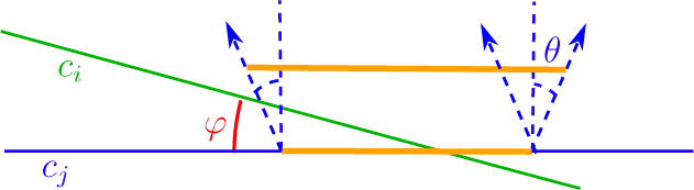


 Open access