


1 Introduction
We consider nonlinear dispersive equations
 $$ \begin{align} \begin{split} & i \partial_t u(t,x) + \mathcal{L}\left(\nabla, \tfrac{1}{\varepsilon}\right) u(t,x) =\vert \nabla\vert^{\alpha} p\left(u(t,x), \overline{u}(t,x)\right)\\ & u(0,x) = v(x), \end{split} \end{align} $$
where we assume a polynomial nonlinearity p and that the structure of (1) implies at least local well-posedness of the problem on a finite time interval $]0,T]$
,
$]0,T]$
, $T<\infty $
in an appropriate functional space. Here, u is the complex-valued solution that we want to approximate. Concrete examples are discussed in Section 5, including the cubic nonlinear Schrödinger (NLS) equation
$T<\infty $
in an appropriate functional space. Here, u is the complex-valued solution that we want to approximate. Concrete examples are discussed in Section 5, including the cubic nonlinear Schrödinger (NLS) equation
 $$ \begin{align} i \partial_t u + \mathcal{L}\left(\nabla\right) u = \vert u\vert^2 u, \quad \mathcal{L}\left(\nabla\right) = \Delta, \end{align} $$
the Korteweg–de Vries (KdV) equation
 $$ \begin{align} \partial_t u +\mathcal{L}\left(\nabla\right) u = \frac12 \partial_x u^2, \quad \mathcal{L}\left(\nabla\right) = i\partial_x^3, \end{align} $$
as well as highly oscillatory Klein–Gordon type systems
 $$ \begin{align} i \partial_t u = -\mathcal{L}\left(\nabla, \tfrac{1}{\varepsilon}\right) u + \frac{1}{\varepsilon^2}\mathcal{L}\left(\nabla, \tfrac{1}{\varepsilon}\right)^{-1} \textstyle p(u,\overline{u}), \quad \mathcal{L}\left(\nabla, \tfrac{1}{\varepsilon}\right) = \frac{1}{\varepsilon}\sqrt{\frac{1}{\varepsilon^2}-\Delta}. \end{align} $$
In the last decades, Strichartz and Bourgain space estimates allowed establishing well-posedness results for dispersive equations in low regularity spaces [Reference Burq, Gérard and Tzvetkov15, Reference Bourgain9, Reference Keel and Tao58, Reference Strichartz77, Reference Tao78]. Numerical theory for dispersive partial differential equations (PDEs), on the other hand, is in general still restricted to smooth solutions. This is due to the fact that most classical approximation techniques were originally developed for linear problems and thus, in general, neglect nonlinear frequency interactions in a system. In the dispersive setting (1) the interaction of the differential operator $\mathcal {L}$
with the nonlinearity p, however, triggers oscillations both in space and in time and, unlike for parabolic problems, no smoothing can be expected. At low regularity and high oscillations, these nonlinear frequency interactions play an essential role: Note that while the influence of
$\mathcal {L}$
with the nonlinearity p, however, triggers oscillations both in space and in time and, unlike for parabolic problems, no smoothing can be expected. At low regularity and high oscillations, these nonlinear frequency interactions play an essential role: Note that while the influence of $i\mathcal {L}$
can be small, the influence of the interaction of
$i\mathcal {L}$
can be small, the influence of the interaction of $+i\mathcal {L}$
and
$+i\mathcal {L}$
and $-i\mathcal {L}$
can be huge and vice versa. Classical linearised frequency approximations, used, for example, in splitting methods or exponential integrators (see Table 1) are therefore restricted to smooth solutions. The latter is not only a technical formality: The severe order reduction in case of nonsmooth solutions is also observed numerically (see, e.g., [Reference Jahnke and Lubich57, Reference Ostermann and Schratz72] and Figure 2), and only very little is known on how to overcome this issue. For an extensive overview on numerical methods for Hamiltonian systems, geometric numerical analysis, structure preserving algorithms and highly oscillatory problems we refer to the books Butcher [Reference Butcher17], Engquist et al. [Reference Engquist, Fokas, Hairer and Iserles36], Faou [Reference Faou37], E. Hairer et al. [Reference Hairer, Nørsett and Wanner46, Reference Hairer, Lubich and Wanner45], Holden et al. [Reference Holden, Karlsen, Lie and Risebro51], Leimkuhler and Reich [Reference Leimkuhler and Reich61], McLachlan and Quispel [Reference McLachlan and Quispel67], Sanz-Serna and Calvo [Reference Sanz-Serna and Calvo75] and the references therein.
$-i\mathcal {L}$
can be huge and vice versa. Classical linearised frequency approximations, used, for example, in splitting methods or exponential integrators (see Table 1) are therefore restricted to smooth solutions. The latter is not only a technical formality: The severe order reduction in case of nonsmooth solutions is also observed numerically (see, e.g., [Reference Jahnke and Lubich57, Reference Ostermann and Schratz72] and Figure 2), and only very little is known on how to overcome this issue. For an extensive overview on numerical methods for Hamiltonian systems, geometric numerical analysis, structure preserving algorithms and highly oscillatory problems we refer to the books Butcher [Reference Butcher17], Engquist et al. [Reference Engquist, Fokas, Hairer and Iserles36], Faou [Reference Faou37], E. Hairer et al. [Reference Hairer, Nørsett and Wanner46, Reference Hairer, Lubich and Wanner45], Holden et al. [Reference Holden, Karlsen, Lie and Risebro51], Leimkuhler and Reich [Reference Leimkuhler and Reich61], McLachlan and Quispel [Reference McLachlan and Quispel67], Sanz-Serna and Calvo [Reference Sanz-Serna and Calvo75] and the references therein.
Table 1 Classical frequency approximations of the principal oscillations (7).

In this work, we establish a new framework of resonance-based approximations for dispersive equations which will allow us to approximate with high-order accuracy a large class of equations under (much) lower regularity assumptions than classical techniques require. The key in the construction of the new methods lies in analysing the underlying oscillatory structure of the system (1). We look at the corresponding mild solution given by Duhamel’s formula
 $$ \begin{align} u(t) = e^{ it \mathcal{L}\left(\nabla, \frac{1}{\varepsilon}\right)} v - ie^{ it \mathcal{L}\left(\nabla, \frac{1}{\varepsilon}\right)}\vert \nabla\vert^\alpha \int_0^t e^{ -i\xi \mathcal{L}\left(\nabla, \frac{1}{\varepsilon}\right)} p\left(u(\xi), \overline{u}(\xi)\right) d\xi \end{align} $$
and its iterations
 $$ \begin{align} u(t) = e^{ it \mathcal{L}\left(\nabla, \frac{1}{\varepsilon}\right)} v - ie^{ it \mathcal{L}\left(\nabla, \frac{1}{\varepsilon}\right)} \vert \nabla\vert^\alpha\mathcal{I}_1( t, \mathcal{L},v,p) +\vert \nabla\vert^{2\alpha} \int_0^t \int_0^\xi \ldots d\xi_1 d \xi. \end{align} $$
The principal oscillatory integral $\mathcal {I}_1( t, \mathcal {L},v,p)$
thereby takes the form
$\mathcal {I}_1( t, \mathcal {L},v,p)$
thereby takes the form
 $$ \begin{align*} \mathcal{I}_1( t, \mathcal{L},v,p) = \int_0^t \mathcal{O}\mathcal{s}\mathcal{c}(\xi, \mathcal{L}, v,p) d\xi \end{align*} $$
with the central oscillations
 $$ \begin{align} \mathcal{O}\mathcal{s}\mathcal{c}(\xi, \mathcal{L}, v,p) = e^{ -i\xi \mathcal{L}\left(\nabla, \frac{1}{\varepsilon}\right)} p\left(e^{ i \xi \mathcal{L}\left(\nabla, \frac{1}{\varepsilon}\right)} v , e^{ - i \xi \mathcal{L}\left(\nabla, \frac{1}{\varepsilon}\right)} \overline{v} \right) \end{align} $$
driven by the nonlinear frequency interactions between the differential operator $\mathcal {L}$
and the nonlinearity p. In order to obtain a suitable approximation at low regularity, it is central to resolve these oscillations – characterised by the underlying structure of resonances – numerically. Classical linearised frequency approximations, however, neglect the nonlinear interactions in (7). This linearisation is illustrated in Table 1 for splitting and exponential integrator methods ([Reference Hairer, Lubich and Wanner45, Reference Hochbruck and Ostermann49]).
$\mathcal {L}$
and the nonlinearity p. In order to obtain a suitable approximation at low regularity, it is central to resolve these oscillations – characterised by the underlying structure of resonances – numerically. Classical linearised frequency approximations, however, neglect the nonlinear interactions in (7). This linearisation is illustrated in Table 1 for splitting and exponential integrator methods ([Reference Hairer, Lubich and Wanner45, Reference Hochbruck and Ostermann49]).
The aim of this article is to introduce a framework which allows us to embed the underlying nonlinear oscillations (7) and their higher-order counterparts into the numerical discretisation. The main idea for tackling this problem is to introduce a decorated tree formalism that optimises the structure of the local error by mapping it to the particular regularity of the solution.
While first-order resonance-based discretisations have been presented for particular examples – for example, the Nonlinear Schrödinger (NLS), Korteweg–de Vries (KdV), Boussinesq, Dirac and Klein–Gordon equation; see [Reference Hofmanová and Schratz50, Reference Baumstark, Faou and Schratz4, Reference Baumstark and Schratz5, Reference Ostermann and Schratz72, Reference Ostermann and Su73, Reference Schratz, Wang and Zhao76] – no general framework could be established so far. Each and every equation had to be targeted carefully one at a time based on a sophisticated resonance analysis. This is due to the fact that the structure of the underlying oscillations (7) strongly depends on the form of the leading operator $\mathcal {L}$
, the nonlinearity p and, in particular, their nonlinear interactions.
$\mathcal {L}$
, the nonlinearity p and, in particular, their nonlinear interactions.
In addition to the lack of a general framework, very little is known about the higher-order counterpart of resonance-based discretisations. Indeed, some attempts have been made for second-order schemes (see, e.g., [Reference Hofmanová and Schratz50] for KdV and [Reference Knöller, Ostermann and Schratz60] for NLS), but they are not optimal. This is due to the fact that the leading differential operator $\mathcal {L} $
triggers a full spectrum of frequencies
$\mathcal {L} $
triggers a full spectrum of frequencies $k_{\kern-1.2pt j} \in {\mathbf {Z}}^{d}$
. Up to now it was an unresolved issue on how to control their nonlinear interactions up to higher order, in particular, in higher spatial dimensions where stability poses a key problem. Even in case of a simple NLS equation it is an open question whether stable low regularity approximations of order higher than one can be achieved in spatial dimensions
$k_{\kern-1.2pt j} \in {\mathbf {Z}}^{d}$
. Up to now it was an unresolved issue on how to control their nonlinear interactions up to higher order, in particular, in higher spatial dimensions where stability poses a key problem. Even in case of a simple NLS equation it is an open question whether stable low regularity approximations of order higher than one can be achieved in spatial dimensions $d\geq 2$
. In particular, previous works suggest a severe order reduction ([Reference Knöller, Ostermann and Schratz60]).
$d\geq 2$
. In particular, previous works suggest a severe order reduction ([Reference Knöller, Ostermann and Schratz60]).
To overcome this, we introduce a new tailored decorated tree formalism. Thereby the decorated trees encode the Fourier coefficients in the iteration of Duhamel’s formula, where the node decoration encodes the frequencies which is in the spirit close to [Reference Christ27, Reference Guo, Kwon and Oh44, Reference Gubinelli43]. The main difficulty then lies in controlling the nonlinear frequency interactions within these iterated integrals up to the desired order with the constraint of a given a priori regularity of the solution. The latter is achieved by embedding the underlying oscillations, and their higher-order iterations, via well-chosen Taylor series expansions into our formalism: The dominant interactions will be embedded exactly, whereas only the lower-order parts are approximated within the discretisation.
We base our algebraic structures on the ones developed for stochastic partial differential equations (SPDEs) with regularity structure [Reference Hairer47] which is a generalisation of rough paths [Reference Lyons63, Reference Lyons64, Reference Gubinelli41, Reference Gubinelli42]. Part of the formalism is inspired by [Reference Bruned, Hairer and Zambotti13] and the recentring map used for giving a local description of the solution of singular SPDEs. We adapt it to the context of dispersive PDEs by using a new class of decorated trees encoding the underlying dominant frequencies.
The framework of decorated trees and the underlying Hopf algebras have allowed the resolution of a large class of singular SPDEs [Reference Hairer47, Reference Bruned, Hairer and Zambotti13, Reference Chandra and Hairer22, Reference Bruned, Chandra, Chevyrev and Hairer11] which include a natural random dynamic on the space of loops in a Riemannian manifold in [Reference Bruned, Gabriel, Hairer and Zambotti12]; see [Reference Bruned, Hairer and Zambotti14] for a very brief survey on these developments. With this general framework, one can study properties of singular SPDEs solutions in full subcritical regimes [Reference Chandra, Hairer and Shen23, Reference Berglund and Bruned6, Reference Hairer and Schönbauer48, Reference Chandra, Moinat and Weber24]. The formalism of decorated trees together with the description of the renormalised equation in this context (see [Reference Bruned, Chandra, Chevyrev and Hairer11]) was directly inspired from numerical analysis of ordinary differential equations (ODEs), more precisely, from the characterisation of Runge–Kutta methods via B-series. Indeed, B-series are numerical (multi-)step methods for ODEs represented by a tree expansion; see, for example, [Reference Butcher16, Reference Berland, Owren and Skaflestad7, Reference Chartier, Hairer and Vilmart26, Reference Hairer, Lubich and Wanner45, Reference Iserles, Quispel and Tse56, Reference Calaque, Ebrahimi-Fard and Manchon19]. We also refer to [Reference Munthe-Kaas and Føllesdal68] for a review of B-series on Lie groups and homogeneous manifolds as well as to [Reference Murua and Sanz-Serna69] providing an alternative structure via word series. The field of singular SPDEs took advantage of the B-series formalism and extended their structures via the adjunction of decorations and Taylor expansions. Now, through this work, numerical analysis is taking advantage of these extended structures and enlarges their scope.
This work proposes a new application of the Butcher–Connes–Kreimer Hopf algebra [Reference Butcher16, Reference Connes and Kreimer31] to dispersive PDEs. It gives a new light on structures that have been used in various fields such as numerical analysis, renormalisation in quantum field theory, singular SPDEs and dynamical systems for classifying singularities via resurgent functions introduced by Jean Ecalle (see [Reference Ecalle34, Reference Fauvet and Menous38]). This is another testimony of the universality of this structure and adds a new object to this landscape. Our construction is motivated by two main features: Taylor expansions that are at the foundation of the numerical scheme (added at the level of the algebra as for singular SPDEs) and the frequency interaction (encoded in a tree structure for dispersive PDEs). The combination of the two together with the Butcher–Connes–Kreimer Hopf algebra allows us to design a novel class of schemes at low regularity. We observe a similar Birkhoff type factorisation as in SPDEs and perturbative quantum field theory. This factorisation allows us to single out oscillations and to perform the local error analysis.
Our main result is the new general resonance-based scheme presented in Definition 4.4 with its error structure given in Theorem 4.8. Our general framework is illustrated on concrete examples in Section 5 and simulations show the efficacy of the scheme. The algebraic structure in Section 2 has its own interest where the main objective is to understand the frequency interactions. The Birkhoff factorisation given in Subsection 3.2 is designed for this purpose and is helpful in proving Theorem 4.8. This factorisation seems new in comparison to the literature.
Assumptions. We impose a periodic boundary condition, $x \in {\mathbf {T}}^d$
. However, our theory can be extended to the full space
$x \in {\mathbf {T}}^d$
. However, our theory can be extended to the full space ${\mathbf {R}}^d$
. We assume that the differential operator
${\mathbf {R}}^d$
. We assume that the differential operator $\mathcal {L}$
is real and consider two types of structures of the system (1) which will allow us to handle dispersive equations at low regularity (such as NLS and KdV) and highly oscillatory Klein–Gordon type systems; see also (2)–(4).
$\mathcal {L}$
is real and consider two types of structures of the system (1) which will allow us to handle dispersive equations at low regularity (such as NLS and KdV) and highly oscillatory Klein–Gordon type systems; see also (2)–(4).
-
• The differential operators $\mathcal {L}\left (\nabla , \frac {1}{\varepsilon }\right ) = \mathcal {L}\left (\nabla \right ) $
and
$\vert \nabla \vert ^\alpha $
cast in Fourier space into the form (8)for some
$$ \begin{align} \mathcal{L}\left(\nabla \right)(k) = k^\sigma + \sum_{\gamma : |\gamma| < \sigma} a_{\gamma} \prod_{j} k_j^{\gamma_j} ,\qquad \vert \nabla\vert^\alpha(k) = \prod_{ \gamma : |\gamma| {\leq \alpha}} k_j^{\gamma_j} \end{align} $$
$ \alpha \in {\mathbf {R}} $
,
$ \gamma \in {\mathbf {Z}}^d $
and
$ |\gamma | = \sum _i \gamma _i $
, where for
$k = (k_1,\ldots ,k_d)\in {\mathbf {Z}}^d$
and
$m = (m_1, \ldots , m_d)\in {\mathbf {Z}}^d$
we set
$$ \begin{align*} k^\sigma = k_1^\sigma + \ldots + k_d^\sigma, \qquad k \cdot m = k_1 m_1 + \ldots + k_d m_d. \end{align*} $$
$\mathcal {L}\left (\nabla , \frac {1}{\varepsilon }\right ) = \mathcal {L}\left (\nabla \right ) $
and
$\vert \nabla \vert ^\alpha $
cast in Fourier space into the form (8)for some
$$ \begin{align} \mathcal{L}\left(\nabla \right)(k) = k^\sigma + \sum_{\gamma : |\gamma| < \sigma} a_{\gamma} \prod_{j} k_j^{\gamma_j} ,\qquad \vert \nabla\vert^\alpha(k) = \prod_{ \gamma : |\gamma| {\leq \alpha}} k_j^{\gamma_j} \end{align} $$
$ \alpha \in {\mathbf {R}} $
,
$ \gamma \in {\mathbf {Z}}^d $
and
$ |\gamma | = \sum _i \gamma _i $
, where for
$k = (k_1,\ldots ,k_d)\in {\mathbf {Z}}^d$
and
$m = (m_1, \ldots , m_d)\in {\mathbf {Z}}^d$
we set
$$ \begin{align*} k^\sigma = k_1^\sigma + \ldots + k_d^\sigma, \qquad k \cdot m = k_1 m_1 + \ldots + k_d m_d. \end{align*} $$
-
• We also consider the setting of a given high frequency
$\frac {1}{\vert \varepsilon \vert } \gg 1$
. In this case we assume that the operators
$\mathcal {L}\left (\nabla , \frac {1}{\varepsilon }\right ) $
and
$\vert \nabla \vert ^\alpha $
take the form (9)for some differential operators
$$ \begin{align} \mathcal{L}\left(\nabla, \frac{1}{\varepsilon}\right) = \frac{1}{\varepsilon^{\sigma}} + \mathcal{B}\left(\nabla, \frac{1}{\varepsilon}\right), \qquad \vert \nabla\vert^\alpha = \mathcal{C}\left(\nabla, \frac{1}{\varepsilon}\right) \end{align} $$
$\mathcal {B}\left (\nabla , \frac {1}{\varepsilon }\right )$
and
$\mathcal {C}\left (\nabla , \frac {1}{\varepsilon }\right )$
which can be bounded uniformly in
$ \vert \varepsilon \vert $
and are relatively bounded by differential operators of degree
$\sigma $
and degree
$\alpha < \sigma $
, respectively. This allows us to include, for instance, highly oscillatory Klein–Gordon type equations (4) (see also Subsection 5.3).


Figure 1 Initial values for Figure 2: $u_0 \in H^1$
(left) and
$u_0 \in H^1$
(left) and $u_0 \in \mathcal {C}^\infty $
(right).
$u_0 \in \mathcal {C}^\infty $
(right).
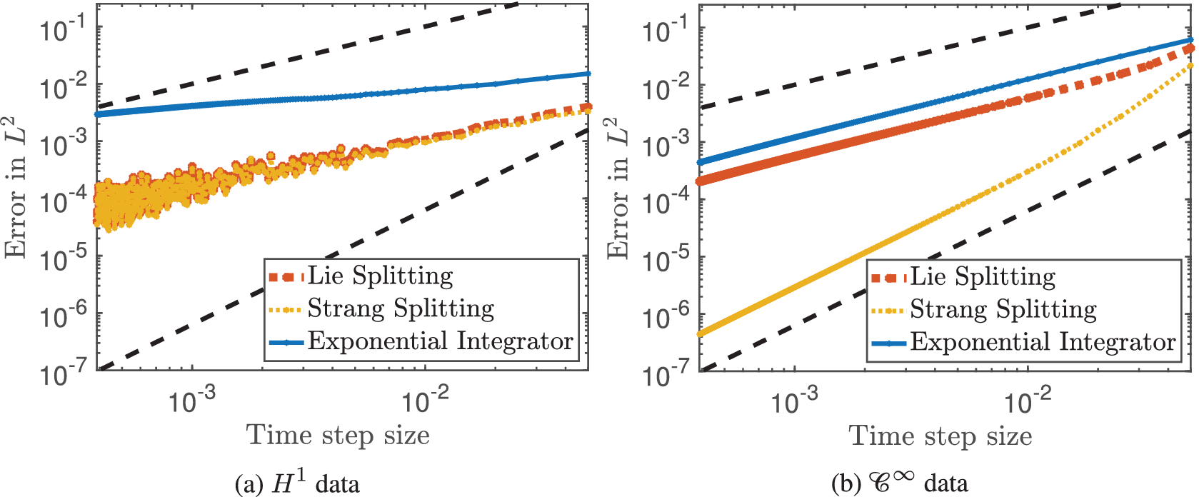
Figure 2 Order reduction of classical schemes based on linearised frequency approximations (cf. Table 1) in case of low regularity data (error versus step size for the cubic Schrödinger equation). For smooth solutions, classical methods reach their full order of convergence (right). In contrast, for less smooth solutions they suffer from severe order reduction (left). The initial values in $H^1$
and
$H^1$
and $\mathcal {C}^{\infty }$
are plotted in Figure 1. The slope of the reference solutions (dashed lines) is one and two, respectively.
$\mathcal {C}^{\infty }$
are plotted in Figure 1. The slope of the reference solutions (dashed lines) is one and two, respectively.
In the next section we introduce the resonance-based techniques to solve the dispersive PDE (1) and illustrate our approach on the example of cubic nonlinear Schrödinger equation (2); see Example 1.
1.1 Resonances as a computational tool
Instead of employing classical linearised frequency approximations (cf. Table 1), we want to embed the underlying nonlinear oscillations
 $$ \begin{align} \mathcal{O}\mathcal{s}\mathcal{c}(\xi, \mathcal{L}, v,p) = e^{ -i\xi \mathcal{L}\left(\nabla, \frac{1}{\varepsilon}\right)} p\left(e^{ i \xi \mathcal{L}\left(\nabla, \frac{1}{\varepsilon}\right)} v , e^{ - i \xi \mathcal{L}\left(\nabla, \frac{1}{\varepsilon}\right)} \overline{v} \right) \end{align} $$
(and their higher-order counterparts) into the numerical discretisation. In case of the 1-dimensional cubic Schrödinger equation (2) the central oscillations (10), for instance, take in Fourier the form (see Example 1 for details)
 $$ \begin{align*}\mathcal{O}\mathcal{s}\mathcal{c}(\xi, \Delta, v,\text{cub}) =\sum_{\substack{k_1,k_2,k_3 \in {\mathbf{Z}}\\-k_1+k_2+k_3 = k} } e^{i k x } \overline{\hat{v}}_{k_1} \hat{v}_{k_2} \hat{v}_{k_3} \int_0^\tau e^{i s \mathscr{F}(k) } ds \end{align*} $$
with the underlying resonance structure
 $$ \begin{align} \mathscr{F}(k) = 2 k_1^2 - 2 k_1 (k_2+k_3) + 2 k_2 k_3. \end{align} $$
Ideally we would like to resolve all nonlinear frequency interactions (11) exactly in our scheme. However, these result in a generalised convolution (of Coifman–Meyer type [Reference Coifman and Meyer30]) which cannot be converted as a product into the physical space. Thus, the iteration would need to be carried out fully in Fourier space which does not yield a scheme which can be practically implemented in higher spatial dimensions; see also Remark 1.3. The latter in general also holds true in the abstract setting (10).
In order to obtain an efficient and practical resonance-based discretisation, we extract the dominant and lower-order parts from the resonance structure (10). More precisely, we filter out the dominant parts $ \mathcal {L}_{\text {dom}}$
and treat them exactly while only approximating the lower-order terms in the spirit of
$ \mathcal {L}_{\text {dom}}$
and treat them exactly while only approximating the lower-order terms in the spirit of
 $$ \begin{align} \mathcal{O}\mathcal{s}\mathcal{c}(\xi, \mathcal{L}, v,p) = \left[e^{i \xi \mathcal{L}_{\text{dom}} \left(\nabla, \frac{1}{\varepsilon}\right)} p_{\text{dom}}\left(v,\overline{v}\right) \right] p_{\text{low}}(v,\overline{v}) + \mathcal{O}\Big(\xi\mathcal{L}_{\text{low}}\left(\nabla\right)v\Big). \end{align} $$
Here, $\mathcal {L}_{\text {dom}}$
denotes a suitable dominant part of the high frequency interactions and
$\mathcal {L}_{\text {dom}}$
denotes a suitable dominant part of the high frequency interactions and
 $$ \begin{align} \mathcal{L}_{\text{low}} = \mathcal{L} - \mathcal{L}_{\text{dom}} \end{align} $$
the corresponding nonoscillatory parts (details will be given in Definition 2.6). The crucial issue is to determine $\mathcal {L}_{\text {dom}}$
,
$\mathcal {L}_{\text {dom}}$
, $p_{\text {dom}}$
and
$p_{\text {dom}}$
and $\mathcal {L}_{\text {low}}, p_{\text {low}}$
in (12) with an interplay between keeping the underlying structure of PDE and allowing a practical implementation at a reasonable cost. We refer to Example 1 for the concrete characterisation in case of cubic NLS, where
$\mathcal {L}_{\text {low}}, p_{\text {low}}$
in (12) with an interplay between keeping the underlying structure of PDE and allowing a practical implementation at a reasonable cost. We refer to Example 1 for the concrete characterisation in case of cubic NLS, where $\mathcal {L}_{\text {low}} = \nabla $
and
$\mathcal {L}_{\text {low}} = \nabla $
and $\mathcal {L}_{\text {dom}} = \Delta $
.
$\mathcal {L}_{\text {dom}} = \Delta $
.
Thanks to the resonance-based ansatz (12), the principal oscillatory integral
 $$ \begin{align*} \mathcal{I}_1( t, \mathcal{L},v,p) = \int_0^t \mathcal{O}\mathcal{s}\mathcal{c}(\xi, \mathcal{L}, v,p) d\xi \end{align*} $$
in the expansion of the exact solution (6)
 $$ \begin{align} u(t) = e^{ it \mathcal{L}\left(\nabla, \frac{1}{\varepsilon}\right)} v - ie^{ it \mathcal{L}\left(\nabla, \frac{1}{\varepsilon}\right)} \vert \nabla\vert^\alpha \mathcal{I}_1( t, \mathcal{L},v,p) + \mathcal{O}\left( t^2\vert \nabla\vert^{2 \alpha}{ q_1( v)} \right) \end{align} $$
(for some polynomial $q_1$
) then takes the form
$q_1$
) then takes the form
 $$ \begin{align} \begin{split} \mathcal{I}_1( t, \mathcal{L},v,p) & = \int_0^t \left[e^{i \xi \mathcal{L}_{\text{dom}}} p_{\text{dom}}\left(v,\overline{v}\right) \right] p_{\text{low}}(v,\overline{v}) + \mathcal{O}\Big(\xi\mathcal{L}_{\text{low}}\left(\nabla\right){ q_2(v)}\Big)d \xi\\ & = t p_{\text{low}}(v,\overline{v}) \varphi_1\left(i t \mathcal{L}_{\text{dom}} \right) p_{\text{dom}}\left(v,\overline{v}\right) + \mathcal{O}\Big(t^2\mathcal{L}_{\text{low}}\left(\nabla\right){ q_2(v)}\Big) \end{split} \end{align} $$
(for some polynomial $q_2$
) where for shortness we write
$q_2$
) where for shortness we write $\mathcal {L} = \mathcal {L}\left (\nabla , \frac {1}{\varepsilon }\right )$
and define
$\mathcal {L} = \mathcal {L}\left (\nabla , \frac {1}{\varepsilon }\right )$
and define $\varphi _1(\gamma ) = \gamma ^{-1}\left (e^\gamma -1\right )$
for
$\varphi _1(\gamma ) = \gamma ^{-1}\left (e^\gamma -1\right )$
for $\gamma \in \mathbf {C}$
. Plugging (15) into (14) yields for a small time step
$\gamma \in \mathbf {C}$
. Plugging (15) into (14) yields for a small time step $\tau $
that
$\tau $
that
 $$ \begin{align} u(\tau) = e^{ i\tau \mathcal{L}} v - \tau ie^{ i\tau \mathcal{L}} \vert \nabla\vert^\alpha &\Big[p_{\text{low}}(v,\overline{v}) \varphi_1\left(i \tau \mathcal{L}_{\text{dom}} \left(\nabla, \frac{1}{\varepsilon}\right)\right) p_{\text{dom}}\left(v,\overline{v}\right) \Big] \notag \\ &\qquad\qquad \qquad + \mathcal{O}\left( \tau^2\vert \nabla\vert^{2 \alpha} q_ 1(v) \right) + \mathcal{O}\Big(\tau^2\vert \nabla\vert^{ \alpha}\mathcal{L}_{\text{low}} \left(\nabla\right)q_2({ v})\Big) \end{align} $$
for some polynomials $q_1, q_2$
. The expansion of the exact solution (16) builds the foundation of the first-order resonance-based discretisation
$q_1, q_2$
. The expansion of the exact solution (16) builds the foundation of the first-order resonance-based discretisation
 $$ \begin{align} u^{n+1} = e^{ i\tau \mathcal{L}} u^n - \tau ie^{ i\tau \mathcal{L}} { \vert \nabla\vert^\alpha} \Big[p_{\text{low}}(u^n,\overline{u}^n) \varphi_1\left(i \tau\mathcal{L}_{\text{dom}} \left(\nabla, \frac{1}{\varepsilon}\right) \right) p_{\text{dom}}\left(u^n,\overline{u}^n\right) \Big]. \end{align} $$
Compared to classical linear frequency approximations (cf. Table 1), the main gain of the more involved resonance-based approach (17) is the following: All dominant parts $\mathcal {L}_{\text {dom}}$
are captured exactly in the discretisation, while only the lower-order/nonoscillatory parts
$\mathcal {L}_{\text {dom}}$
are captured exactly in the discretisation, while only the lower-order/nonoscillatory parts $\mathcal {L}_{\text {low}}$
are approximated. Henceforth, within the resonance-based approach (17) the local error only depends on the lower-order, nonoscillatory operator
$\mathcal {L}_{\text {low}}$
are approximated. Henceforth, within the resonance-based approach (17) the local error only depends on the lower-order, nonoscillatory operator $\mathcal {L}_{\text {low}}$
, while the local error of classical methods involves the full operator
$\mathcal {L}_{\text {low}}$
, while the local error of classical methods involves the full operator $\mathcal {L}$
and, in particular, its dominant part
$\mathcal {L}$
and, in particular, its dominant part $\mathcal {L}_{\text {dom}}$
. Thus, the resonance-based approach (17) allows us to approximate a more general class of solutions
$\mathcal {L}_{\text {dom}}$
. Thus, the resonance-based approach (17) allows us to approximate a more general class of solutions
 $$ \begin{align} &u \in \underbrace{ \mathcal{D}\left(\vert \nabla\vert^\alpha \mathcal{L}_{\text{low}}\left(\nabla, \frac{1}{\varepsilon}\right)\right) }_{\text{resonance domain}} \cap \mathcal{D}\left(\vert \nabla\vert^{2\alpha}\right) \notag \\ &\qquad \qquad \supset { \mathcal{D}\left(\vert \nabla\vert^\alpha \mathcal{L}\left(\nabla, \frac{1}{\varepsilon}\right)\right) }\cap \mathcal{D}\left(\vert \nabla\vert^{2\alpha}\right) =\underbrace{ \mathcal{D}\left(\vert \nabla\vert^\alpha \mathcal{L}_{\text{dom}}\left(\nabla, \frac{1}{\varepsilon}\right)\right) }_{\text{classical domain}}\cap \mathcal{D}\left(\vert \nabla\vert^{2\alpha}\right). \end{align} $$
Higher-order resonance-based methods. Classical approximation techniques, such as splitting or exponential integrator methods, can easily be extended to higher order; see, for example, [Reference Hairer, Lubich and Wanner45, Reference Hochbruck and Ostermann49, Reference Thalhammer80]. The step from a first- to higher-order approximation lies in subsequently employing a higher-order Taylor series expansion to the exact solution
 $$ \begin{align*} u(t) = u(0) + t\partial_t u(0) + \ldots + \frac{t^{r}}{r!} \partial_t^{r} u(0) + \mathcal{O} \left( t^{r+1} \partial_{t}^{r+1} u\right). \end{align*} $$
Within this expansion, the higher-order iterations of the oscillations (7) in the exact solution are, however, not resolved but subsequently linearised. Therefore, classical high-order methods are restricted to smooth solutions as their local approximation error in general involves high-order derivatives
 $$ \begin{align} \mathcal{O} \left( t^{r+1} \partial_{t}^{r+1} u\right)=\mathcal{O} \left( t^{r+1} \mathcal{L}^{r+1}\left(\nabla, \tfrac{1}{\varepsilon}\right) u\right). \end{align} $$
This phenomenon is also illustrated in Figure 2 where we numerically observe the order reduction of the Strang splitting method (of classical order 2) down to the order of the Lie splitting method (of classical order 1) in case of rough solutions. In particular, we observe that classical high-order methods do not pay off at low regularity as their error behaviour reduces to the one of lower-order methods.
At first glance our resonance-based approach can also be straightforwardly extended to higher order. Instead of considering only the first-order iteration (6) the natural idea is to iterate Duhamel’s formula (5) up to the desired order r; that is, for initial value $u(0)=v$
,
$u(0)=v$
,
 $$ \begin{align} \begin{split} u(t) &= e^{i t \mathcal{L}} v -i e^{i t \mathcal{L}}\nabla^{\alpha} \int_0^te^{ -i \xi_1 \mathcal{L}} p\left( e^{ i \xi_1 \mathcal{L}} v,e^{- i \xi_1 \mathcal{L}} \overline{v}\right) d\xi_1 \\ &\quad{}-e^{i t \mathcal{L}}\nabla^{\alpha} \int_0^te^{ -i \xi_1 \mathcal{L}} \Big[D_1 p \left( e^{ i \xi_1 \mathcal{L}} v,e^{- i \xi_1 \mathcal{L}} \overline{v}\right) \\ &\quad \cdot e^{ i \xi_1\mathcal{L}}\nabla^{\alpha} \int_0^{\xi_1} e^{ -i \xi_2 \mathcal{L}} p\left( e^{ i \xi_1 \mathcal{L}} v,e^{- i \xi_1 \mathcal{L}} \overline{v}\right) d\xi_2 \Big]d\xi_1 \\ &\quad{}+e^{i t \mathcal{L}}\nabla^{\alpha} \int_0^te^{ -i \xi_1 \mathcal{L}} \Big[D_2p \left( e^{ i \xi_1 \mathcal{L}} v,e^{- i \xi_1 \mathcal{L}} \overline{v}\right) \\ & \quad{} \cdot e^{ -i \xi_1\mathcal{L}}\nabla^{\alpha} \int_0^{\xi_1} e^{ i \xi_2 \mathcal{L}} \overline{p\left( e^{ i \xi_1 \mathcal{L}} v,e^{- i \xi_1 \mathcal{L}} \overline{v}\right) }d\xi_2 \Big]d\xi_1 \\ & \quad{}+ \ldots+\nabla^{\alpha} \int_0^t\nabla^{\alpha} \int_0^\xi \ldots \nabla^{\alpha}\int_0^{\xi_r} d\xi_{r} \ldots d\xi_1 d \xi \end{split} \end{align} $$
where $ D_1 $
(respectively
$ D_1 $
(respectively $ D_2 $
) corresponds to the derivative in the first (respectively second) component of
$ D_2 $
) corresponds to the derivative in the first (respectively second) component of $ p $
. The key idea will then be the following: Instead of linearising the frequency interactions by a simple Taylor series expansion of the oscillatory terms
$ p $
. The key idea will then be the following: Instead of linearising the frequency interactions by a simple Taylor series expansion of the oscillatory terms $e^{\pm i \xi _\ell \mathcal {L}}$
(as classical methods would do), we want to embed the dominant frequency interactions of (20) exactly into our numerical discretisation. By neglecting the last term involving the iterated integral of order r, we will then introduce the desired local error
$e^{\pm i \xi _\ell \mathcal {L}}$
(as classical methods would do), we want to embed the dominant frequency interactions of (20) exactly into our numerical discretisation. By neglecting the last term involving the iterated integral of order r, we will then introduce the desired local error $\mathcal {O}\Big (\nabla ^{(r+1)\alpha } t^{r+1}q(u)\Big )$
for some polynomial q.
$\mathcal {O}\Big (\nabla ^{(r+1)\alpha } t^{r+1}q(u)\Big )$
for some polynomial q.
Compared to the first-order approximation (12), this is much more involved as high-order iterations of the nonlinear frequency interactions need to be controlled. The control of these iterated oscillations is not only a delicate problem on the discrete (numerical) level, concerning accuracy, stability, etc., but already on the continuous level: We have to encode the structure (which strongly depends on the underlying structure of the PDE; that is, the form of operator $\mathcal {L}$
and the shape of nonlinearity p) and at the same time keep track of the regularity assumptions. In order to achieve this in the general setting (1), we will introduce the decorated tree formalism in Subsection 1.2. First, let us first illustrate the main ideas on the example of the cubic periodic Schrödinger equation.
$\mathcal {L}$
and the shape of nonlinearity p) and at the same time keep track of the regularity assumptions. In order to achieve this in the general setting (1), we will introduce the decorated tree formalism in Subsection 1.2. First, let us first illustrate the main ideas on the example of the cubic periodic Schrödinger equation.
Example 1 (cubic periodic Schrödinger equation). We consider the 1-dimensional cubic Schrödinger equation
 $$ \begin{align} i \partial_t u + \partial_x^2 u = \vert u\vert^2 u \end{align} $$
equipped with periodic boundary conditions; that is, $x \in {\mathbf {T}}$
. The latter casts into the general form (1) with
$x \in {\mathbf {T}}$
. The latter casts into the general form (1) with
 $$ \begin{align} \mathcal{L}\left(\nabla, \tfrac{1}{\varepsilon}\right) = \partial_x^2, \quad \alpha = 0 \quad \text{and}\quad p(u,\overline{u}) =u^2 \overline{u}. \end{align} $$
In the case of cubic NLS, the central oscillatory integral (at first order) takes the form (cf. (7))
 $$ \begin{align} \mathcal{I}_1(\tau, \partial_x^2,v) = \int_0^\tau e^{-i s \partial_x^2}\left[ \left( e^{- i s \partial_x^2} \overline{v} \right) \left ( e^{ i s \partial_x^2} v \right)^2\right] d s. \end{align} $$
Assuming that $v\in L^2$
, the Fourier transform
$v\in L^2$
, the Fourier transform $ v(x) = \sum _{k \in {\mathbf {Z}}}\hat {v}_k e^{i k x} $
allows us to express the action of the free Schrödinger group as a Fourier multiplier; that is,
$ v(x) = \sum _{k \in {\mathbf {Z}}}\hat {v}_k e^{i k x} $
allows us to express the action of the free Schrödinger group as a Fourier multiplier; that is,
 $$ \begin{align*} e^{\pm i t \partial_x^2}v(x) = \sum_{k \in {\mathbf{Z}}} e^{\mp i t k^2} \hat{v}_k e^{i k x}. \end{align*} $$
With this at hand, we can express the oscillatory integral (23) as follows:
 $$ \begin{align} \mathcal{I}_1(\tau, \partial_x^2,v) = \sum_{\substack{k_1,k_2,k_3 \in {\mathbf{Z}} \\ -k_1+k_2+k_3 = k} } e^{i k x } \overline{\hat{v}}_{k_1} \hat{v}_{k_2} \hat{v}_{k_3} \int_0^\tau e^{i s \mathscr{F}(k) } ds \end{align} $$
with the underlying resonance structure
 $$ \begin{align}{ \mathscr{F}(k) = 2 k_1^2 - 2 k_1 (k_2+k_3) + 2 k_2 k_3}. \end{align} $$
In the spirit of (12) we need to extract the dominant and lower-order parts from the resonance structure (25). The choice is based on the following observation. Note that $2k_1^2$
corresponds to a second-order derivative; that is, with the inverse Fourier transform
$2k_1^2$
corresponds to a second-order derivative; that is, with the inverse Fourier transform $\mathcal {F}^{\,-1}$
, we have
$\mathcal {F}^{\,-1}$
, we have
 $$ \begin{align*} \mathcal{F}^{-1}\left(2k_1^2 \overline{\hat v}_{k_1} \hat v_{k_2} \hat v_{k_3}\right) = \left(- 2\partial_x^2 \overline{v}\right) v^2 \end{align*} $$
while the terms $k_\ell \cdot k_m$
with
$k_\ell \cdot k_m$
with $\ell \neq m$
correspond only to first-order derivatives; that is,
$\ell \neq m$
correspond only to first-order derivatives; that is,
 $$ \begin{align*} \mathcal{F}^{-1}\left(k_1 \overline{\hat v}_{k_1} k_2 \hat v_{k_2} \hat v_{k_3}\right) = -\vert\partial_x v\vert^2 v, \quad \mathcal{F}^{-1}\left( \overline{\hat v}_{k_1} k_2 \hat v_{k_2} k_3 \hat v_{k_3}\right) = - (\partial_x v)^2\overline{v}. \end{align*} $$
This motivates the choice
 $$ \begin{align*} \mathscr{F}(k) = \mathcal{L}_{\text{dom}}(k_1) + \mathcal{L}_{\text{low}}(k_1,k_2,k_3) \end{align*} $$
with
 $$ \begin{align} {\mathcal{L}_{\text{dom}}(k_1) = 2k_1^2 \quad \text{and}\quad \mathcal{L}_{\text{low}}(k_1,k_2,k_3) = - 2 k_1 (k_2+k_3) + 2 k_2 k_3}. \end{align} $$
In terms of (17) we thus have
 $$ \begin{align} \mathcal{L}_{\text{dom}} = - 2\partial_x^2, \quad \quad p_{\text{dom}}(v,\overline{v}) = \overline{v} \quad \text{and}\quad p_{\text{low}}(v,\overline{v}) = v^2 \end{align} $$
and the first-order NLS resonance-based discretisation (17) takes the form
 $$ \begin{align} u^{n+1} = e^{ i\tau \partial_x^2} u^n - \tau ie^{ i\tau \partial_x^2} \Big[(u^n)^2 \varphi_1\left(-2 i \tau \partial_x^2 \right) \overline{u}^n \Big]. \end{align} $$
Thanks to (16), we readily see by (26) that the NLS scheme (28) introduces the approximation error
 $$ \begin{align} \mathcal{O}\left(\tau^2 \mathcal{L}_{\text{low}}q(u)\right)= \mathcal{O}\left(\tau^2 \partial_xq(u)\right) \end{align} $$
for some polynomial q in u. Compared to the error structure of classical discretisation techniques, which involve the full and thus dominant operator $\mathcal {L}_{\text {dom}} = \partial _x^2$
, we thus gain one derivative with the resonance-based scheme (28). This favourable error at low regularity is underlined in Figure 3.
$\mathcal {L}_{\text {dom}} = \partial _x^2$
, we thus gain one derivative with the resonance-based scheme (28). This favourable error at low regularity is underlined in Figure 3.
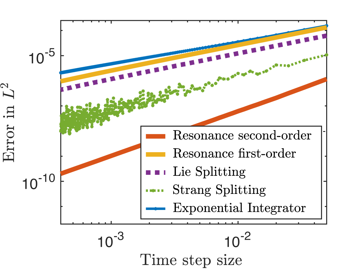
Figure 3 Error versus step size (double logarithmic plot). Comparison of classical and resonance-based schemes for the cubic Schrödinger equation (21) with $H^2$
initial data.
$H^2$
initial data.
In Example 1 we illustrated the idea of the resonance-based discretisation on the cubic periodic Schrödinger equation in one spatial dimension. In order to control frequency interactions in the general setting (1) in arbitrary dimensions $d\geq 1$
up to arbitrary high order, we next introduce our decorated tree formalism.
$d\geq 1$
up to arbitrary high order, we next introduce our decorated tree formalism.
1.2 Main idea of decorated trees for high-order resonance-based schemes
The iteration of Duhamel’s formulation (20) can be expressed using decorated trees. We are interested in computing the iterated frequency interactions in (20). This motivates us to express the latter in Fourier space. Let $ r $
be the order of the scheme and let us assume that we truncate (20) at this order. Its kth Fourier coefficient at order
$ r $
be the order of the scheme and let us assume that we truncate (20) at this order. Its kth Fourier coefficient at order $ r $
is given by
$ r $
is given by
 $$ \begin{align} U_{k}^{r}(\tau, v) = \sum_{T\kern-1pt\in\kern0.5pt {\cal V}^r_k} \frac{\Upsilon^{p}(T)(v)}{S(T)} \left( \Pi T \right)(\tau), \end{align} $$
where $ {\cal V}^r_k $
is a set of decorated trees which incorporate the frequency k,
$ {\cal V}^r_k $
is a set of decorated trees which incorporate the frequency k, $ S(T) $
is the symmetry factor associated to the tree
$ S(T) $
is the symmetry factor associated to the tree $ T $
,
$ T $
, $ \Upsilon ^{p}(T) $
is the coefficient appearing in the iteration of Duhamel’s formulation and
$ \Upsilon ^{p}(T) $
is the coefficient appearing in the iteration of Duhamel’s formulation and $ (\Pi T)(t) $
represents a Fourier iterated integral. The exponent r in
$ (\Pi T)(t) $
represents a Fourier iterated integral. The exponent r in $ {\cal V}^r_k $
means that we consider only trees of size
$ {\cal V}^r_k $
means that we consider only trees of size $ r +1 $
which are the trees producing an iterated integral with
$ r +1 $
which are the trees producing an iterated integral with $ r + 1$
integrals. The decorations that need to be put on the trees are illustrated in Example 2.
$ r + 1$
integrals. The decorations that need to be put on the trees are illustrated in Example 2.
The main difficulty then lies in developing for every $T \in {\cal V}^r_k$
a suitable approximation to the iterated integrals
$T \in {\cal V}^r_k$
a suitable approximation to the iterated integrals $ (\Pi T)(t) $
with the aim of minimising the local error structure (in the sense of regularity). In order to achieve this, the key idea is to embed – in the spirit of (12) – the underlying resonance structure of the iterated integrals
$ (\Pi T)(t) $
with the aim of minimising the local error structure (in the sense of regularity). In order to achieve this, the key idea is to embed – in the spirit of (12) – the underlying resonance structure of the iterated integrals $ (\Pi T)(t) $
into the discretisation.
$ (\Pi T)(t) $
into the discretisation.
Example 2
(cubic periodic Schrödinger equation with decorated trees). When $r=2$
, decorated trees for cubic NLS are given by
$r=2$
, decorated trees for cubic NLS are given by

where on the nodes we encode the frequencies such that they add up depending on the edge decorations. The root has no decoration. For example, in $T_1$
the two extremities of the blue edge have the same decoration given by
$T_1$
the two extremities of the blue edge have the same decoration given by $ -k_1 + k_2 + k_3 $
where the minus sign comes from the dashed edge. Therefore,
$ -k_1 + k_2 + k_3 $
where the minus sign comes from the dashed edge. Therefore, $ {\cal V}^r_k $
contains infinitely many trees (finitely many shapes but infinitely many ways of splitting up the frequency
$ {\cal V}^r_k $
contains infinitely many trees (finitely many shapes but infinitely many ways of splitting up the frequency $ k $
among the branches). An edge of type
$ k $
among the branches). An edge of type
![]() encodes a multiplication by
encodes a multiplication by $ e^{-i \tau k^2} $
where k is the frequency on the nodes adjacent to this edge. An edge of type
$ e^{-i \tau k^2} $
where k is the frequency on the nodes adjacent to this edge. An edge of type
![]() encodes an integration in time of the form
encodes an integration in time of the form
 $$ \begin{align*} \int_0^{\tau} e^{i s k^2} \cdots d s. \end{align*} $$
In fact, $r +1$
, the truncation parameter, corresponds to the maximum number of integration in time; that is, the number of edges with type
$r +1$
, the truncation parameter, corresponds to the maximum number of integration in time; that is, the number of edges with type
![]() . The dashed dots on the edges correspond to a conjugate and a multiplication by
. The dashed dots on the edges correspond to a conjugate and a multiplication by $(-1)$
applied to the frequency at the top of this edge. Then, if we apply the map
$(-1)$
applied to the frequency at the top of this edge. Then, if we apply the map $ \Pi $
(which encodes the oscillatory integrals in Fourier space; see Subsection 3.1) to these trees, we obtain
$ \Pi $
(which encodes the oscillatory integrals in Fourier space; see Subsection 3.1) to these trees, we obtain
 $$ \begin{align} \begin{split} (\Pi T_0)(\tau) & = e^{-i \tau k^2}, \\ (\Pi T_1)(\tau) & = - i e^{-i \tau k^2} \int_0^\tau e^{i s k^2}\left[ \left( e^{ i s k_1^2} \right) \left ( e^{ -i s k_2^2} \right) \left ( e^{ -i s k_3^2} \right) \right] d s \\ & = - i e^{-i \tau k^2} \int_0^{\tau} e^{is \mathscr{F}(k)} ds \\ (\Pi T_2)(\tau) & = -i e^{-i \tau k^2} \int_0^\tau e^{i s k^2}\left[ \left( e^{ i s k_4^2} \right) \Big( (\Pi T_1)(s) \Big) \left ( e^{ - i s k_5^2} \right) \right] d s \\ (\Pi T_3)(\tau) & = -i e^{-i \tau k^2} \int_0^\tau e^{i s k^2}\left[ \Big( \overline{(\Pi T_1)(s)} \Big)\left ( e^{ -i s k_4^2} \right) \left ( e^{ -i s k_5^2} \right) \right] d s \end{split} \end{align} $$
where the resonance structure $\mathscr {F}(k)$
is given in (25). One has the constraints
$\mathscr {F}(k)$
is given in (25). One has the constraints $k= -k_1 +k_2 +k_3$
for
$k= -k_1 +k_2 +k_3$
for $T_1$
,
$T_1$
, $k= -k_1 + k_2 + k_3 -k_4 + k_5$
for
$k= -k_1 + k_2 + k_3 -k_4 + k_5$
for $ T_2 $
and
$ T_2 $
and $k= k_1 - k_2 - k_3 +k_4 + k_5$
for
$k= k_1 - k_2 - k_3 +k_4 + k_5$
for $ T_3 $
. Using the definitions in Section 4, one can compute the following coefficients:
$ T_3 $
. Using the definitions in Section 4, one can compute the following coefficients:
 $$ \begin{align*} \begin{split} \frac{\Upsilon^p(T_0)(v)}{S(T_0)} & = \hat v_k, \quad \frac{\Upsilon^p(T_1)(v)}{S(T_1)} = \bar{\hat{v}}_{k_1} \hat{v}_{k_2} \hat{v}_{k_3} \\ \frac{\Upsilon^p(T_2)(v)}{S(T_2)} & = 2 \overline{\hat{v}}_{k_1} \hat v_{k_2} \hat v_{k_3} \overline{\hat{v}}_{k_4} \hat v_{k_5}, \quad \frac{\Upsilon^p(T_3)(v)}{S(T_3)} = \hat v_{k_1} \overline{\hat{v}}_{k_2} \overline{\hat{v}}_{k_3} \hat v_{k_4} \hat v_{k_5} \end{split} \end{align*} $$
which together with the character $ \Pi $
encode fully the identity (30).
$ \Pi $
encode fully the identity (30).
Our general scheme is based on the approximation of $(\Pi T)(t)$
for every tree in
$(\Pi T)(t)$
for every tree in ${\cal V}_k^r$
. This approximation is given by a new map of decorated trees denoted by
${\cal V}_k^r$
. This approximation is given by a new map of decorated trees denoted by $\Pi ^{n,r}$
where r is the order of the scheme and n corresponds to the a priori assumed regularity of the initial value v. This new character
$\Pi ^{n,r}$
where r is the order of the scheme and n corresponds to the a priori assumed regularity of the initial value v. This new character $\Pi ^{n,r}$
will embed the dominant frequency interactions and neglect the lower-order terms in the spirit of (12). Our general scheme will thus take the form
$\Pi ^{n,r}$
will embed the dominant frequency interactions and neglect the lower-order terms in the spirit of (12). Our general scheme will thus take the form
 $$ \begin{align} U_{k}^{n,r}(\tau, v) = \sum_{T\kern-1pt\in\kern0.5pt {\cal V}^r_k} \frac{\Upsilon^{p}(T)(v)}{S(T)} \left( \Pi^{n,r} T \right)(\tau) \end{align} $$
where the map $ \Pi ^{n,r} T $
is a low regularity approximation of order
$ \Pi ^{n,r} T $
is a low regularity approximation of order $ r $
of the map
$ r $
of the map $ \Pi T $
in the sense that
$ \Pi T $
in the sense that
 $$ \begin{align} \left(\Pi T - \Pi^{n,r} T \right)(\tau) = \mathcal{O}\left( \tau^{r+2} \mathcal{L}^{r}_{\tiny{\text{low}}}(T,n) \right). \end{align} $$
Here $\mathcal {L}^{r}_{\tiny {\text {low}}}(T,n)$
involves all lower-order frequency interactions that we neglect in our resonance-based discretisation. At first order this approximation is illustrated in (15). The scheme (33) and the local error approximations (34) are the main results of this work (see Theorem 4.8). Let us give the main ideas on how to obtain them.
$\mathcal {L}^{r}_{\tiny {\text {low}}}(T,n)$
involves all lower-order frequency interactions that we neglect in our resonance-based discretisation. At first order this approximation is illustrated in (15). The scheme (33) and the local error approximations (34) are the main results of this work (see Theorem 4.8). Let us give the main ideas on how to obtain them.
The approximation $ \Pi ^{n,r} $
is constructed from a character
$ \Pi ^{n,r} $
is constructed from a character $ \Pi ^n $
defined on the vector space
$ \Pi ^n $
defined on the vector space $ {\mathcal {H}} $
spanned by decorated forests taking values in a space
$ {\mathcal {H}} $
spanned by decorated forests taking values in a space $ {{\cal C}} $
which depends on the frequencies of the decorated trees (see, e.g., (31) in case of NLS). However, we will add at the root the additional decoration r which stresses that this tree will be an approximation of order r. For this purpose we will introduce the symbol
$ {{\cal C}} $
which depends on the frequencies of the decorated trees (see, e.g., (31) in case of NLS). However, we will add at the root the additional decoration r which stresses that this tree will be an approximation of order r. For this purpose we will introduce the symbol ${\cal D}^r$
(see, e.g., (35) for
${\cal D}^r$
(see, e.g., (35) for $T_1$
of NLS). Indeed, we disregard trees which have more integrals in time than the order of the scheme. In particular, we note that
$T_1$
of NLS). Indeed, we disregard trees which have more integrals in time than the order of the scheme. In particular, we note that $ \Pi ^n {\cal D}^r(T) = \Pi ^{n,r} T$
.
$ \Pi ^n {\cal D}^r(T) = \Pi ^{n,r} T$
.
The map $ \Pi ^n $
is defined recursively from an operator
$ \Pi ^n $
is defined recursively from an operator $ {{\cal K}} $
which will compute a suitable approximation (matching the regularity of the solution) of the integrals introduced by the iteration of Duhamel’s formula. This map
$ {{\cal K}} $
which will compute a suitable approximation (matching the regularity of the solution) of the integrals introduced by the iteration of Duhamel’s formula. This map $ {{\cal K}} $
corresponds to the high-order counterpart of the approach described in Subsection 1.1: It embeds the idea of singling out the dominant parts and integrating them exactly while only approximating the lower-order terms, allowing for an improved local error structure compared to classical approaches. The character
$ {{\cal K}} $
corresponds to the high-order counterpart of the approach described in Subsection 1.1: It embeds the idea of singling out the dominant parts and integrating them exactly while only approximating the lower-order terms, allowing for an improved local error structure compared to classical approaches. The character $ \Pi ^n $
is the main map for computing the numerical scheme in Fourier space.
$ \Pi ^n $
is the main map for computing the numerical scheme in Fourier space.
Example 3
(cubic periodic Schrödinger equation: computation of $\Pi ^n$
). We consider the decorated trees
$\Pi ^n$
). We consider the decorated trees ${\cal D}^r(\bar T_1)$
and
${\cal D}^r(\bar T_1)$
and $\bar T_1$
given by
$\bar T_1$
given by

One can observe that $ (\Pi T_1)(t) = e^{-i k^2 t} (\Pi \bar T_1)(t). $
We will define recursively two maps
$ (\Pi T_1)(t) = e^{-i k^2 t} (\Pi \bar T_1)(t). $
We will define recursively two maps $\mathscr {F}_{\tiny {\text {dom}}} $
and
$\mathscr {F}_{\tiny {\text {dom}}} $
and $ \mathscr {F}_{\tiny {\text {low}}} $
(see Definition 2.6) on decorated trees that compute the dominant and the lower part of the nonlinear frequency interactions within the oscillatory integral
$ \mathscr {F}_{\tiny {\text {low}}} $
(see Definition 2.6) on decorated trees that compute the dominant and the lower part of the nonlinear frequency interactions within the oscillatory integral $ (\Pi \bar T_1)(t) $
. In this example, one gets back the values already computed in (26); that is,
$ (\Pi \bar T_1)(t) $
. In this example, one gets back the values already computed in (26); that is,
 $$ \begin{align*} \mathscr{F}_{\tiny{\text{dom}}}(\bar T_1) = \mathcal{L}_{\tiny{\text{dom}}}(k_1), \quad \mathscr{F}_{\tiny{\text{low}}}(\bar T_1) =\mathcal{L}_{\tiny{\text{low}}}(k_1,k_2,k_3). \end{align*} $$
Moreover, the dominant part of $T_1$
is due to the observation that
$T_1$
is due to the observation that $(\Pi T_1)(t) = e^{-i k^2 t} (\Pi \bar T_1)(t)$
given by
$(\Pi T_1)(t) = e^{-i k^2 t} (\Pi \bar T_1)(t)$
given by
 $$ \begin{align*} \mathscr{F}_{\tiny{\text{dom}}}( T_1) = -k^2 +\mathscr{F}_{\tiny{\text{dom}}}(\bar T_1) , \end{align*} $$
because the tree $T_1$
does not start with an intregral in time. Then, one can write
$T_1$
does not start with an intregral in time. Then, one can write
 $$ \begin{align*} (\Pi \bar T_1)(t) = -i \int_0^\tau e^{i s\mathscr{F}_{\tiny{\text{dom}}}(\bar T_1) } e^{i s\mathscr{F}_{\tiny{\text{low}}}(\bar T_1) } ds \end{align*} $$
and Taylor expand around $0$
the lower-order term; that is, the factor containing
$0$
the lower-order term; that is, the factor containing $ \mathscr {F}_{\tiny {\text {low}}}(\bar T_1)$
. The term
$ \mathscr {F}_{\tiny {\text {low}}}(\bar T_1)$
. The term $\Pi ^{n,1} \bar T_1 = \Pi ^n {\cal D}^1(\bar T_1)$
is then given by
$\Pi ^{n,1} \bar T_1 = \Pi ^n {\cal D}^1(\bar T_1)$
is then given by
 $$ \begin{align} ( \Pi^{n,1} \bar T_1)(t) = - i \int_0^\tau e^{i s\mathscr{F}_{\tiny{\text{dom}}}(\bar T_1) } ds + \mathscr{F}_{\tiny{\text{low}}}(\bar T_1) \int_0^\tau s e^{i s \mathscr{F}_{\tiny{\text{dom}}}(\bar T_1) } ds. \end{align} $$
One observes that we obtain terms of the form $ \frac {P}{Q} e^{i R} $
where
$ \frac {P}{Q} e^{i R} $
where $P,Q, R$
are polynomials in the frequencies
$P,Q, R$
are polynomials in the frequencies $ k_1, k_2, k_3 $
. Linear combinations of these terms are actually the definition of the space
$ k_1, k_2, k_3 $
. Linear combinations of these terms are actually the definition of the space $ {{\cal C}} $
. For the local error, one gets
$ {{\cal C}} $
. For the local error, one gets
 $$ \begin{align} ( \Pi^{n,1} \bar T_1)(t) - ( \Pi \bar T_1)(t) = {{\cal O}}( t^3 \mathscr{F}_{\tiny{\text{low}}} (\bar T_1)^2 ). \end{align} $$
Here the term $ \mathscr {F}_{\tiny {\text {low}}} (\bar T_1)^2$
corresponds to the regularity that one has to impose on the solution. One can check by hand that the expression of
$ \mathscr {F}_{\tiny {\text {low}}} (\bar T_1)^2$
corresponds to the regularity that one has to impose on the solution. One can check by hand that the expression of $ \Pi ^{n,1} \bar T_1$
can be mapped back to the physical space. Such a statement will in general hold true for the character
$ \Pi ^{n,1} \bar T_1$
can be mapped back to the physical space. Such a statement will in general hold true for the character $ \Pi ^n $
; see Proposition 3.18. This will be important for the practical implementation of the new schemes; see also Remark 1.3. We have not used n in the description of the scheme yet. In fact, it plays a role in the expression of
$ \Pi ^n $
; see Proposition 3.18. This will be important for the practical implementation of the new schemes; see also Remark 1.3. We have not used n in the description of the scheme yet. In fact, it plays a role in the expression of $ \Pi ^{n,1} \bar T_1 $
. One has to compare
$ \Pi ^{n,1} \bar T_1 $
. One has to compare $ n $
with the regularity required by the local error (37) introduced by the polynomial
$ n $
with the regularity required by the local error (37) introduced by the polynomial $ \mathscr {F}_{\tiny {\text {low}}} (\bar T_1)^2 $
but also with the term
$ \mathscr {F}_{\tiny {\text {low}}} (\bar T_1)^2 $
but also with the term $\mathscr {F}_{\tiny {\text {dom}}}(\bar T_1)^2 $
. Indeed, if the initial value is regular enough, we may want to Taylor expand all of the frequencies – that is, even the dominant parts – in order to get a simpler scheme; see also Remark 1.1.
$\mathscr {F}_{\tiny {\text {dom}}}(\bar T_1)^2 $
. Indeed, if the initial value is regular enough, we may want to Taylor expand all of the frequencies – that is, even the dominant parts – in order to get a simpler scheme; see also Remark 1.1.
In order to obtain a better understanding of the error introduced by the character $ \Pi ^n $
, one needs to isolate each interaction. Therefore, we will introduce two characters
$ \Pi ^n $
, one needs to isolate each interaction. Therefore, we will introduce two characters $ \hat \Pi ^n : {\mathcal {H}} \rightarrow {{\cal C}} $
and
$ \hat \Pi ^n : {\mathcal {H}} \rightarrow {{\cal C}} $
and $ A^n : {\mathcal {H}} \rightarrow \mathbf {C} $
such that
$ A^n : {\mathcal {H}} \rightarrow \mathbf {C} $
such that
 $$ \begin{align} \Pi^n = \left( \hat \Pi^n \otimes A^n \right) \Delta \end{align} $$
where $ \Delta : {\mathcal {H}} \rightarrow {\mathcal {H}} \otimes {\mathcal {H}}_+ $
is a coaction and
$ \Delta : {\mathcal {H}} \rightarrow {\mathcal {H}} \otimes {\mathcal {H}}_+ $
is a coaction and $ ({\mathcal {H}},\Delta ) $
is a right comodule for a Hopf algebra
$ ({\mathcal {H}},\Delta ) $
is a right comodule for a Hopf algebra $ {\mathcal {H}}_+ $
equipped with a coproduct
$ {\mathcal {H}}_+ $
equipped with a coproduct ${\Delta ^{\!+}} $
and an antipode
${\Delta ^{\!+}} $
and an antipode $ {\mathcal {A}} $
. In fact, on can show that
$ {\mathcal {A}} $
. In fact, on can show that
 $$ \begin{align} \hat \Pi^n = \left( \Pi^n \otimes \left( {\mathcal{Q}} \circ \Pi^n {\mathcal{A}} \cdot \right)(0) \right) \Delta, \quad A^n = ({\mathcal{Q}} \circ \Pi^n \cdot)(0) \end{align} $$
where $ \Pi ^n $
is extended to a character on
$ \Pi ^n $
is extended to a character on $ {\mathcal {H}}_+ $
and
$ {\mathcal {H}}_+ $
and $ {\mathcal {Q}} $
is a projection defined on
$ {\mathcal {Q}} $
is a projection defined on $ {{\cal C}} $
which keeps only the terms with no oscillations. The identity (39) can be understood as a Birkhoff type factorisation of
$ {{\cal C}} $
which keeps only the terms with no oscillations. The identity (39) can be understood as a Birkhoff type factorisation of $ \hat \Pi ^n $
using the character
$ \hat \Pi ^n $
using the character $ \Pi ^n $
. This identity is also reminiscent in the main results obtained for singular SPDEs [Reference Bruned, Hairer and Zambotti13] where two twisted antipodes play a fundamental role providing a variant of the algebraic Birkhoff factorisation.
$ \Pi ^n $
. This identity is also reminiscent in the main results obtained for singular SPDEs [Reference Bruned, Hairer and Zambotti13] where two twisted antipodes play a fundamental role providing a variant of the algebraic Birkhoff factorisation.
Example 4 (cubic periodic Schrödinger equation: Birkhoff factorisation). Integrating the first term in (36) exactly yields two contributions:
 $$ \begin{align*} \int_0^\tau e^{i s\mathscr{F}_{\tiny{\text{dom}}}(\bar T_1) } ds = \frac{e^{i\tau\mathscr{F}_{\tiny{\text{dom}}}(\bar T_1) }}{i\mathscr{F}_{\tiny{\text{dom}}}(\bar T_1) } - \frac{1}{i\mathscr{F}_{\tiny{\text{dom}}}(\bar T_1) }. \end{align*} $$
Plugging these two terms into $(\Pi T_2)(\tau )$
defined in (32), we see that we have to control the following two terms:
$(\Pi T_2)(\tau )$
defined in (32), we see that we have to control the following two terms:
 $$ \begin{align} \begin{split} - e^{-i \tau k^2} & \int_0^\tau e^{i s k^2}\left[ \left( e^{ i s k_4^2} \right) \Big( \frac{e^{i s\mathscr{F}_{\tiny{\text{dom}}}(\bar T_1) - is \bar k^2 } }{i\mathscr{F}_{\tiny{\text{dom}}}(\bar T_1) } \Big) \left ( e^{- i s k_5^2} \right) \right] d s \\ - e^{-i \tau k^2} & \int_0^\tau e^{-i s k^2}\left[ \left( e^{ i s k_4^2} \right) \Big( - \frac{e^{-i s \bar k^2 }}{i\mathscr{F}_{\tiny{\text{dom}}}(\bar T_1) } \Big) \left ( e^{ -i s k_5^2} \right) \right] d s \end{split} \end{align} $$
where $ \bar k = -k_1 + k_2 + k_3$
. The frequency analysis is needed again for approximating the time integral and defining an approximation of
$ \bar k = -k_1 + k_2 + k_3$
. The frequency analysis is needed again for approximating the time integral and defining an approximation of $(\Pi T_2)(\tau ) $
. One can see that the dominant part of these two terms may differ. This implies that one can get two different local errors for the approximation of these two terms; the final local error is the maximum between the two. At this point, we need an efficient algebraic structure for dealing with all of these frequency interactions in the iterated integrals. We first consider a character
$(\Pi T_2)(\tau ) $
. One can see that the dominant part of these two terms may differ. This implies that one can get two different local errors for the approximation of these two terms; the final local error is the maximum between the two. At this point, we need an efficient algebraic structure for dealing with all of these frequency interactions in the iterated integrals. We first consider a character $ \hat \Pi ^n $
that keeps only the main contribution; that is, the second term of (40). For any decorated tree
$ \hat \Pi ^n $
that keeps only the main contribution; that is, the second term of (40). For any decorated tree $ T $
, one expects
$ T $
, one expects $ \hat \Pi ^n $
to be of the form
$ \hat \Pi ^n $
to be of the form
 $$ \begin{align*} (\hat \Pi^n {\cal D}^r(T))(t) = B^n({\cal D}^r(T))(t) e^{it\mathscr{F}_{\tiny{\text{dom}}}( T) } \end{align*} $$
where $ B^n({\cal D}^r(T))(t) $
is a polynomial in
$ B^n({\cal D}^r(T))(t) $
is a polynomial in $ t $
depending on the decorated tree
$ t $
depending on the decorated tree $ T $
. The character
$ T $
. The character $ \hat \Pi ^n $
singles out oscillations by keeping at each iteration only the nonzero one. This separation between the various oscillations can be encoded via the Butcher–Connes–Kreimer coaction
$ \hat \Pi ^n $
singles out oscillations by keeping at each iteration only the nonzero one. This separation between the various oscillations can be encoded via the Butcher–Connes–Kreimer coaction $ \Delta : {\mathcal {H}} \rightarrow {\mathcal {H}} \otimes {\mathcal {H}}_+ $
. An example of computation is given below:
$ \Delta : {\mathcal {H}} \rightarrow {\mathcal {H}} \otimes {\mathcal {H}}_+ $
. An example of computation is given below:

where $ \ell = - k_1 + k_2 + k_3$
. The space
$ \ell = - k_1 + k_2 + k_3$
. The space ${\mathcal {H}}_+$
corresponds to the forest of planted trees where for each planted tree the edge connecting the root to the rest of the tree must be blue (an integration in time). Only blue edges are cut (located on the right-hand side of the tensor product) and the trunk is on the left-hand side. The extra terms missing in the computation correspond to the higher-order terms introduced by the Taylor approximation. Indeed, one plays with decorations introducing an mth derivative on the blue edges cut denoted by
${\mathcal {H}}_+$
corresponds to the forest of planted trees where for each planted tree the edge connecting the root to the rest of the tree must be blue (an integration in time). Only blue edges are cut (located on the right-hand side of the tensor product) and the trunk is on the left-hand side. The extra terms missing in the computation correspond to the higher-order terms introduced by the Taylor approximation. Indeed, one plays with decorations introducing an mth derivative on the blue edges cut denoted by $ \hat {\cal D}^{(r,m)} $
and decorations on the nodes where the edges were previously attached. A node of the form
$ \hat {\cal D}^{(r,m)} $
and decorations on the nodes where the edges were previously attached. A node of the form

in the example above corresponds to the frequency $ \ell $
and the monomial
$ \ell $
and the monomial $ \lambda $
. The length of the Taylor extension is dictated by the order of the scheme
$ \lambda $
. The length of the Taylor extension is dictated by the order of the scheme $ r $
. The operator
$ r $
. The operator $ \hat {\cal D}^{(r,m)} $
is nonzero only if
$ \hat {\cal D}^{(r,m)} $
is nonzero only if $ m \leq r+1 $
. The formulae (38) and (3.8) give the relation between
$ m \leq r+1 $
. The formulae (38) and (3.8) give the relation between $ \Pi ^n $
and
$ \Pi ^n $
and $ \hat \Pi ^n $
which can be interpreted as a Birkhoff factorisation with the explicit formula (3.8) for
$ \hat \Pi ^n $
which can be interpreted as a Birkhoff factorisation with the explicit formula (3.8) for $ A^n $
. Such a factorisation is new and does not seem to have an equivalent in the literature. It is natural to observe this factorisation in this context: The integration in time
$ A^n $
. Such a factorisation is new and does not seem to have an equivalent in the literature. It is natural to observe this factorisation in this context: The integration in time $\int ^{t}_0 \ldots ds$
gives two different frequency interactions that can be controlled via a projection
$\int ^{t}_0 \ldots ds$
gives two different frequency interactions that can be controlled via a projection $ {\mathcal {Q}} $
which needs to be iterated deeper in the tree. This will be the equivalent of the Rota–Baxter map used for such a type of factorisation.
$ {\mathcal {Q}} $
which needs to be iterated deeper in the tree. This will be the equivalent of the Rota–Baxter map used for such a type of factorisation.
The coproduct $ {\Delta ^{\!+}} $
and the coaction
$ {\Delta ^{\!+}} $
and the coaction $ \Delta $
are extremely close in spirit to the ones defined for the recentring in [Reference Hairer47, Reference Bruned, Hairer and Zambotti13]. Indeed, for designing a numerical scheme, we need to perform Taylor expansions, and these two maps perform them at the level of the algebra. The main difference with the tools used for singular SPDEs [Reference Bruned, Hairer and Zambotti13] is the length of the Taylor expansion which is now dictated by the order of the scheme.
$ \Delta $
are extremely close in spirit to the ones defined for the recentring in [Reference Hairer47, Reference Bruned, Hairer and Zambotti13]. Indeed, for designing a numerical scheme, we need to perform Taylor expansions, and these two maps perform them at the level of the algebra. The main difference with the tools used for singular SPDEs [Reference Bruned, Hairer and Zambotti13] is the length of the Taylor expansion which is now dictated by the order of the scheme.
The structure we propose in Section 2 is new and reveals the universality of deformed Butcher–Connes–Kreimer coproducts which appear in [Reference Bruned, Hairer and Zambotti13]. The nondeformed version of this map comes from the analysis of B-series in [Reference Butcher16, Reference Chartier, Hairer and Vilmart26, Reference Calaque, Ebrahimi-Fard and Manchon19], which is itself an extension of the Connes–Kreimer Hopf algebra of rooted trees [Reference Connes and Kreimer31, Reference Connes and Kreimer32] arising in perturbative quantum field theory (QFT) and noncommutative geometry.
One can notice that our approximation $ \Pi ^{n,r} $
depends on
$ \Pi ^{n,r} $
depends on $ n $
which has to be understood as the regularity we assume a priori on the solution. We design our framework such that for smooth solutions the numerical schemes are simplified, recovering in the limit classical linearised approximations as in Table 1.
$ n $
which has to be understood as the regularity we assume a priori on the solution. We design our framework such that for smooth solutions the numerical schemes are simplified, recovering in the limit classical linearised approximations as in Table 1.
Remark 1.1. The term $ \mathcal {L}^{r}_{\tiny {\text {low}}}(T,n) $
in the approximation (34) is obtained by performing several Taylor expansions. Depending on the value
$ \mathcal {L}^{r}_{\tiny {\text {low}}}(T,n) $
in the approximation (34) is obtained by performing several Taylor expansions. Depending on the value $ n $
, we get different numerical schemes (see also the applications in Section 5). In the sequel, we focus on two specific values of
$ n $
, we get different numerical schemes (see also the applications in Section 5). In the sequel, we focus on two specific values of $ n $
associated to two particular schemes. We consider
$ n $
associated to two particular schemes. We consider $ n^{r}_{\tiny {\text {low}}}(T) $
and
$ n^{r}_{\tiny {\text {low}}}(T) $
and $ n^{r}_{\tiny {\text {full}}}(T) $
given by
$ n^{r}_{\tiny {\text {full}}}(T) $
given by
 $$ \begin{align*} n^{r}_{\tiny{\text{low}}}(T) = \deg(\mathcal{L}^{r}_{\tiny{\text{low}}}(T)), \quad n^{r}_{\tiny{\text{full}}}(T) = \deg(\mathcal{L}^{r}_{\tiny{\text{full}}}(T)), \end{align*} $$
where $ \mathcal {L}^{r}_{\tiny {\text {low}}}(T) $
corresponds to the error obtained when we integrate exactly the dominant part
$ \mathcal {L}^{r}_{\tiny {\text {low}}}(T) $
corresponds to the error obtained when we integrate exactly the dominant part $ \mathcal {L}_{\tiny {\text {dom}}}(T)$
and Taylor expand only the lower-order part
$ \mathcal {L}_{\tiny {\text {dom}}}(T)$
and Taylor expand only the lower-order part $ \mathcal {L}_{\tiny {\text {low}}}(T) $
, while the term
$ \mathcal {L}_{\tiny {\text {low}}}(T) $
, while the term $\mathcal {L}^{r}_{\tiny {\text {full}}}(T)$
corresponds to the error one obtains when we Taylor expand the full operator
$\mathcal {L}^{r}_{\tiny {\text {full}}}(T)$
corresponds to the error one obtains when we Taylor expand the full operator $\mathcal {L}(T) = \mathcal {L}_{\tiny {\text {dom}}}(T) + \mathcal {L}_{\tiny {\text {low}}}(T) $
. One has
$\mathcal {L}(T) = \mathcal {L}_{\tiny {\text {dom}}}(T) + \mathcal {L}_{\tiny {\text {low}}}(T) $
. One has
 $$ \begin{align} \deg(\mathcal{L}^{r}_{\tiny{\text{low}}}(T,n)) = \left\{ \begin{array}{lll} \displaystyle n^{r}_{\tiny{\text{low}}}(T), & \quad \text{if }\displaystyle \, n \leq n^{r}_{\tiny{\text{low}}}(T) , \\[2pt] n, & \quad \text{if }\displaystyle \, n^{r}_{\tiny{\text{low}}}(T) \leq n \leq n^{r}_{\tiny{\text{full}}}(T) , \\[2pt] \displaystyle n^{r}_{\tiny{\text{full}}}(T), & \quad \text{if }\displaystyle \, n \geq n^{r}_{\tiny{\text{full}}}(T). \\ \end{array} \right. \end{align} $$
At the level of the scheme, we get
 $$ \begin{align} \Pi^{n,r} T = \left\{ \begin{array}{lll} \displaystyle \Pi_{\tiny{\text{low}}}^{r} T, & \quad \text{if }\displaystyle \, n \leq n^{r}_{\tiny{\text{low}}}(T) , \\[2pt] \displaystyle \Pi^{n,r} T , & \quad \text{if }\displaystyle \, n^{r}_{\tiny{\text{low}}}(T) \leq n \leq n^{r}_{\tiny{\text{full}}}(T) , \\[2pt] \displaystyle \Pi_{\tiny{\text{full}}}^{r} T , & \quad \text{if } \displaystyle \, n \geq n^{r}_{\tiny{\text{full}}}(T) \\ \end{array} \right. \end{align} $$
where we call $ \Pi _{\tiny {\text {low}}}^{r} T $
the minimum regularity resonance-based scheme. This scheme corresponds to the minimisation of the local error and we can observe a plateau. Indeed, if
$ \Pi _{\tiny {\text {low}}}^{r} T $
the minimum regularity resonance-based scheme. This scheme corresponds to the minimisation of the local error and we can observe a plateau. Indeed, if $ n $
is too small, then by convention we get this scheme. This could be the case if one does not compute the minimum regularity needed a priori.
$ n $
is too small, then by convention we get this scheme. This could be the case if one does not compute the minimum regularity needed a priori.
The other scheme $ \Pi _{\tiny {\text {full}}}^{r} T $
corresponds to a classical exponential type discretisation, where enough regularity is assumed such that the dominant components of the iterated integrals can also be expanded into a Taylor series as in (19). Then, we observe a second plateau: indeed, assuming more regularity will not change the scheme as we have already Taylor-expanded all the components.
$ \Pi _{\tiny {\text {full}}}^{r} T $
corresponds to a classical exponential type discretisation, where enough regularity is assumed such that the dominant components of the iterated integrals can also be expanded into a Taylor series as in (19). Then, we observe a second plateau: indeed, assuming more regularity will not change the scheme as we have already Taylor-expanded all the components.
Compared to $ \Pi _{\tiny {\text {low}}}^{r} T $
, the scheme
$ \Pi _{\tiny {\text {low}}}^{r} T $
, the scheme $ \Pi _{\tiny {\text {full}}}^{r} T $
is in general much simpler as no nonlinear frequency interactions are taken into account. This comes at the cost that a smaller class of equations can be solved as much higher regularity assumptions are imposed.
$ \Pi _{\tiny {\text {full}}}^{r} T $
is in general much simpler as no nonlinear frequency interactions are taken into account. This comes at the cost that a smaller class of equations can be solved as much higher regularity assumptions are imposed.
Between these two schemes lies a large class of intermediate schemes $ \Pi ^{n,r} T $
which we call low regularity resonance-based schemes. They take advantage of Taylor expanding a bit more when more regularity is assumed. Therefore, the complexity of the schemes is decreasing as
$ \Pi ^{n,r} T $
which we call low regularity resonance-based schemes. They take advantage of Taylor expanding a bit more when more regularity is assumed. Therefore, the complexity of the schemes is decreasing as $n $
increases; see also Section 5. We can represent these different regimes through the diagram below.
$n $
increases; see also Section 5. We can represent these different regimes through the diagram below.

Remark 1.2. Within our framework we propose a stabilisation technique. This will allow us to improve previous higher-order attempts breaking formerly imposed order barriers of higher-order resonance-based schemes, such as the order reduction down to $3/2$
suggested for Schrödinger equations in dimensions
$3/2$
suggested for Schrödinger equations in dimensions $d\geq 2$
in [Reference Knöller, Ostermann and Schratz60]. Details are given in Remark 3.2 as well as Section 5.
$d\geq 2$
in [Reference Knöller, Ostermann and Schratz60]. Details are given in Remark 3.2 as well as Section 5.
Remark 1.3. The aim is to choose the central approximation $\Pi ^{n,r} T$
as an interplay between optimising the local error in the sense of regularity while allowing for a practical implementation. We design our schemes in such a way that products of functions can always be mapped back to physical space. In practical computations, this will allow us to benefit from the fast Fourier transform (FFT) with computational effort of order
$\Pi ^{n,r} T$
as an interplay between optimising the local error in the sense of regularity while allowing for a practical implementation. We design our schemes in such a way that products of functions can always be mapped back to physical space. In practical computations, this will allow us to benefit from the fast Fourier transform (FFT) with computational effort of order $\mathcal {O}\left (\vert K\vert ^d \text {log}\vert K\vert ^d\right )$
in dimension d, where K denotes the highest frequency in the discretisation. However, it comes at the cost that the approximation error (34) involves lower-order derivatives. If, on the other hand, we would embed all nonlinear frequency interactions into the discretisation, the resulting schemes would need to be carried out fully in Fourier space, causing large memory and computational effort of order
$\mathcal {O}\left (\vert K\vert ^d \text {log}\vert K\vert ^d\right )$
in dimension d, where K denotes the highest frequency in the discretisation. However, it comes at the cost that the approximation error (34) involves lower-order derivatives. If, on the other hand, we would embed all nonlinear frequency interactions into the discretisation, the resulting schemes would need to be carried out fully in Fourier space, causing large memory and computational effort of order $\mathcal {O}\left (K^{d \cdot \text {deg}{p}}\right )$
, where
$\mathcal {O}\left (K^{d \cdot \text {deg}{p}}\right )$
, where $\text {deg}(p)$
denotes the degree of the nonlinearity p.
$\text {deg}(p)$
denotes the degree of the nonlinearity p.
Remark 1.4. For notational simplicity, we focus on equations with polynomial nonlinearities (cf. (1)). Nevertheless, our scheme (33) allows for a generalisation to nonpolynomial nonlinearities of type
 $$ \begin{align*}f(u) g(\overline{u})\end{align*} $$
for smooth functions f and g. In the latter case, the iteration of Duhamel’s formula boils down to a two-step algorithm. More precisely, imagine that we got a first expansion of the form $ e^{i s\mathcal {L}} v + A(v,s) $
where
$ e^{i s\mathcal {L}} v + A(v,s) $
where $ A(v,s) $
is a linear combination of iterated integrals. Then, when iterating Duhamel’s formula we need to plug this expansion into the nonlinearity and perform a Taylor expansion around the point
$ A(v,s) $
is a linear combination of iterated integrals. Then, when iterating Duhamel’s formula we need to plug this expansion into the nonlinearity and perform a Taylor expansion around the point $ e^{is \mathcal {L}}v $
:
$ e^{is \mathcal {L}}v $
:
 $$ \begin{align*} f(e^{i s\mathcal{L}} v + A(v,s)) = \sum_{m \leq r} \frac{A(v,s)^m}{m!} f^{(m)}(e^{i s\mathcal{L}} v ) + \mathcal{O}(A(v,s)^{r+1}). \end{align*} $$
Carrying out the same manipulation for $ g(\overline {e^{i s\mathcal {L}} v + A(v,s)}), $
we end up with terms of type
$ g(\overline {e^{i s\mathcal {L}} v + A(v,s)}), $
we end up with terms of type
 $$ \begin{align*}\frac{A(v,s)^m}{m!} f^{(m)}(e^{i s\mathcal{L}} v ) \frac{\overline{A(v,s)}^n}{n!} g^{(n)}({e^{- i s\mathcal{L}}\overline{v}}). \end{align*} $$
At this point we cannot directly write down our resonance-based scheme due to the fact that the oscillations are still encapsulated inside $ f $
and g. In order to control these oscillations and their nonlinear interactions, we need to pull the oscillatory phases
$ f $
and g. In order to control these oscillations and their nonlinear interactions, we need to pull the oscillatory phases $ e^{\pm is\mathcal {L}} $
out of f and g. This is achieved via expansions of the form
$ e^{\pm is\mathcal {L}} $
out of f and g. This is achieved via expansions of the form
 $$ \begin{align*} f(e^{is \mathcal{L}}v) = \sum_{\ell \leq r} \frac{s^{\ell}}{\ell!} e^{is \mathcal{L}} \mathcal{C}^{\ell}[f,\mathcal{L}](v) + \mathcal{O}(s^{r+1} \mathcal{C}^{r+1}[f,\mathcal{L}](v)) \end{align*} $$
where $\mathcal {C}^{\ell }[f,\mathcal {L}]$
denote nested commutators which in general require (much) less regularity than powers of the full operator
$\mathcal {C}^{\ell }[f,\mathcal {L}]$
denote nested commutators which in general require (much) less regularity than powers of the full operator $\mathcal {L}^\ell $
. After these two linearisation steps, we are able to use the same machinery that leads to the construction of our scheme (33).
$\mathcal {L}^\ell $
. After these two linearisation steps, we are able to use the same machinery that leads to the construction of our scheme (33).
Such commutators were also recently exploited in [Reference Rousset and Schratz74] for second-order methods.
1.3 Outline of the article
Let us give a short review of the content of this article. In Section 2, we introduce the general algebraic framework by first defining a suitable vector space of decorated forests $ \hat {\mathcal {H}} $
. Next, we define the dominant frequencies of a decorated forest (see Definition 2.6) and show that one can map them back into physical space (see Corollary 2.9), which will be important for the efficiency of the numerical schemes (cf. Remark 1.3). Then, we introduced two spaces of decorated forests
$ \hat {\mathcal {H}} $
. Next, we define the dominant frequencies of a decorated forest (see Definition 2.6) and show that one can map them back into physical space (see Corollary 2.9), which will be important for the efficiency of the numerical schemes (cf. Remark 1.3). Then, we introduced two spaces of decorated forests $ {\mathcal {H}}_+ $
and
$ {\mathcal {H}}_+ $
and ${\mathcal {H}}$
. The latter
${\mathcal {H}}$
. The latter $ {\mathcal {H}} $
is used for describing approximated iterated integrals. The main difference with the previous space is that now we project along the order
$ {\mathcal {H}} $
is used for describing approximated iterated integrals. The main difference with the previous space is that now we project along the order $ r $
of the method. We define the maps for the coaction
$ r $
of the method. We define the maps for the coaction $ \Delta : {\mathcal {H}} \rightarrow {\mathcal {H}} \otimes {\mathcal {H}}_+ $
and the coproduct
$ \Delta : {\mathcal {H}} \rightarrow {\mathcal {H}} \otimes {\mathcal {H}}_+ $
and the coproduct $ {\Delta ^{\!+}} : {\mathcal {H}}_+ \rightarrow {\mathcal {H}}_+ \otimes {\mathcal {H}}_+ $
in (65) and (66). In addition, we provide a recursive definition for them in (69). We prove in Proposition 2.15 that these maps give a right-comodule structure for
$ {\Delta ^{\!+}} : {\mathcal {H}}_+ \rightarrow {\mathcal {H}}_+ \otimes {\mathcal {H}}_+ $
in (65) and (66). In addition, we provide a recursive definition for them in (69). We prove in Proposition 2.15 that these maps give a right-comodule structure for $ {\mathcal {H}} $
over the Hopf algebra
$ {\mathcal {H}} $
over the Hopf algebra $ {\mathcal {H}}_+ $
. Moreover, we get a simple expression for the antipode
$ {\mathcal {H}}_+ $
. Moreover, we get a simple expression for the antipode $ {\mathcal {A}} $
in Proposition 80.
$ {\mathcal {A}} $
in Proposition 80.
In Section 3, we construct the approximation of the iterated integrals given by the character $ \Pi : \hat {\mathcal {H}} \rightarrow {{\cal C}} $
(see (82)) through the character
$ \Pi : \hat {\mathcal {H}} \rightarrow {{\cal C}} $
(see (82)) through the character $ \Pi ^n : {\mathcal {H}} \rightarrow {{\cal C}} $
(see (83)). The main operator used for the recursive construction is
$ \Pi ^n : {\mathcal {H}} \rightarrow {{\cal C}} $
(see (83)). The main operator used for the recursive construction is $ {{\cal K}} $
given in Definition 3.1. We introduce a new character
$ {{\cal K}} $
given in Definition 3.1. We introduce a new character $ \hat \Pi ^n : {\mathcal {H}} \rightarrow {{\cal C}} $
through a Birkhoff type factorisation obtained from the character
$ \hat \Pi ^n : {\mathcal {H}} \rightarrow {{\cal C}} $
through a Birkhoff type factorisation obtained from the character $ \Pi ^n $
(see Proposition 3.8). Thanks to
$ \Pi ^n $
(see Proposition 3.8). Thanks to $ \hat \Pi ^n $
, we are able to conduct the local error analysis and show one of the main results of the article: the error estimate on the difference between
$ \hat \Pi ^n $
, we are able to conduct the local error analysis and show one of the main results of the article: the error estimate on the difference between $ \Pi $
and its approximation
$ \Pi $
and its approximation $ \Pi ^n $
(see Theorem 3.17). In Section 4, we introduce decorated trees stemming from Duhamel’s formula via the rules formalism (see Definition 4.2). Then, we are able to introduce the general scheme (see Definition 115) and conclude on its local error structure (see Theorem 4.8).
$ \Pi ^n $
(see Theorem 3.17). In Section 4, we introduce decorated trees stemming from Duhamel’s formula via the rules formalism (see Definition 4.2). Then, we are able to introduce the general scheme (see Definition 115) and conclude on its local error structure (see Theorem 4.8).
In Section 5 we illustrate the general framework on various applications and conclude in Subsection 5.4 with numerical experiments underlying the favourable error behaviour of the new resonance-based schemes for nonsmooth and, in certain cases, even for smooth solutions.
2 General framework
In this section, we present the main algebraic framework which will allow us to develop and analyse our general numerical scheme. We start by introducing decorated trees that encode the oscillatory integrals. Decorations on the edges represent integrals in time and some operators stemming from Duhamel’s formula. In addition, we impose decorations on the nodes for the frequencies and potential monomials. We will compute the corresponding dominant and lower-order frequency interactions associated to these trees via the recursive maps $\mathscr {F}_{\tiny {\text {dom}}} $
and
$\mathscr {F}_{\tiny {\text {dom}}} $
and $ \mathscr {F}_{\tiny {\text {low}}} $
given in Definition 2.6. These maps are chosen such that the solution is approximated at low regularity in Fourier space with the additional property that the approximation can be mapped back to physical space. The latter will allow for an efficient practical implementation of the new scheme, see Remark 1.3.
$ \mathscr {F}_{\tiny {\text {low}}} $
given in Definition 2.6. These maps are chosen such that the solution is approximated at low regularity in Fourier space with the additional property that the approximation can be mapped back to physical space. The latter will allow for an efficient practical implementation of the new scheme, see Remark 1.3.
The second part of this section focuses on a different space of decorated trees that we name approximated decorated trees. The main difference from the trees previously introduced is the additional root decoration by some integer $ r $
. The approximated trees have to be understood as an abstract version of an approximation of order
$ r $
. The approximated trees have to be understood as an abstract version of an approximation of order $ r $
of the corresponding oscillatory integral. In order to construct our low regularity scheme we want to carry out an abstract Taylor expansions of the time integrals at the level of these approximated trees in the spirit of (12): We will Taylor expand only the lower parts of the frequency interactions while integrating the dominant part exactly. For these operations, we need a deformed Butcher–Connes–Kreimer coproduct in the spirit of the one which has been introduced for singular SPDEs. We consider a coproduct
$ r $
of the corresponding oscillatory integral. In order to construct our low regularity scheme we want to carry out an abstract Taylor expansions of the time integrals at the level of these approximated trees in the spirit of (12): We will Taylor expand only the lower parts of the frequency interactions while integrating the dominant part exactly. For these operations, we need a deformed Butcher–Connes–Kreimer coproduct in the spirit of the one which has been introduced for singular SPDEs. We consider a coproduct ${\Delta ^{\!+}} $
and a coaction
${\Delta ^{\!+}} $
and a coaction $ \Delta $
with a nonrecursive (see (65) and (66)) and a recursive definition (see (69)). We show the usual coassociativity/compatibility properties in Proposition 2.14. In the end we get a Hopf algebra and a comodule structures on these new spaces of approximated decorated trees. The antipode comes for free in this context since the Hopf algebra is connected, see Proposition 2.15. The main novelty of this general algebraic framework is the merging of two different structures that appear in dispersive PDEs (frequency interactions) and singular SPDEs (abstract Taylor expansion). They form the central part of the scheme – controlling the underlying oscillations and performing Taylor approximations. Within this construction we need to introduce new objects that were not considered before in such generality.
$ \Delta $
with a nonrecursive (see (65) and (66)) and a recursive definition (see (69)). We show the usual coassociativity/compatibility properties in Proposition 2.14. In the end we get a Hopf algebra and a comodule structures on these new spaces of approximated decorated trees. The antipode comes for free in this context since the Hopf algebra is connected, see Proposition 2.15. The main novelty of this general algebraic framework is the merging of two different structures that appear in dispersive PDEs (frequency interactions) and singular SPDEs (abstract Taylor expansion). They form the central part of the scheme – controlling the underlying oscillations and performing Taylor approximations. Within this construction we need to introduce new objects that were not considered before in such generality.
2.1 Decorated trees and frequency interactions
We consider a set of decorated trees following the formalism developed in [Reference Bruned, Hairer and Zambotti13]. These trees will encode the Fourier coefficients of the numerical scheme.
We assume a finite set $ {\mathfrak {L}}$
and frequencies
$ {\mathfrak {L}}$
and frequencies $ k_1,\ldots ,k_n \in {\mathbf {Z}}^{d} $
. The set
$ k_1,\ldots ,k_n \in {\mathbf {Z}}^{d} $
. The set $ {\mathfrak {L}}$
parametrises a set of differential operators with constant coefficients, whose symbols are given by the polynomials
$ {\mathfrak {L}}$
parametrises a set of differential operators with constant coefficients, whose symbols are given by the polynomials $ (P_{{\mathfrak {t}}})_{{\mathfrak {t}} \in {\mathfrak {L}}} $
. We define the set of decorated trees
$ (P_{{\mathfrak {t}}})_{{\mathfrak {t}} \in {\mathfrak {L}}} $
. We define the set of decorated trees $ \hat {\mathcal {T}} $
as elements of the form
$ \hat {\mathcal {T}} $
as elements of the form $ T_{{\mathfrak {e}}}^{{\mathfrak {n}}, {\mathfrak {f}}} = (T,{\mathfrak {n}},{\mathfrak {f}},{\mathfrak {e}}) $
where
$ T_{{\mathfrak {e}}}^{{\mathfrak {n}}, {\mathfrak {f}}} = (T,{\mathfrak {n}},{\mathfrak {f}},{\mathfrak {e}}) $
where
-
•
$ T $
is a nonplanar rooted tree with root
$ \varrho _T $
, node set
$N_T$
and edge set
$E_T$
. We denote the leaves of
$ T $
by
$ L_T $
.
$ T $
must also be a planted tree, which means that there is only one edge outgoing the root. -
• The map
$ {\mathfrak {e}} : E_T \rightarrow {\mathfrak {L}} \times \lbrace 0,1\rbrace $
are edge decorations. -
• The map
$ {\mathfrak {n}} : N_T \setminus \lbrace \varrho _T \rbrace \rightarrow \mathbf {N} $
are node decorations. For every inner node
$ v$
, this map encodes a monomial of the form
$ \xi ^{{\mathfrak {n}}(v)} $
where
$ \xi $
is a time variable. -
• The map
$ {\mathfrak {f}} : N_T \setminus \lbrace \varrho _T \rbrace \rightarrow {\mathbf {Z}}^{d}$
are node decorations. These decorations are frequencies that satisfy for every inner node
$ u $
: (43)where
$$ \begin{align} (-1)^{\mathfrak{p}(e_u)}{\mathfrak{f}}(u) = \sum_{e=(u,v) \in E_T} (-1)^{\mathfrak{p}(e)} {\mathfrak{f}}(v) \end{align} $$
$ {\mathfrak {e}}(e) = ({\mathfrak {t}}(e),\mathfrak {p}(e)) $
and
$ e_u $
is the edge outgoing
$ u $
of the form
$ (v,u) $
. From this definition, one can see that the node decorations
$ ({\mathfrak {f}}(u))_{u \in L_T} $
determine the decoration of the inner nodes. We assume that the node decorations at the leaves are linear combinations of the
$ k_i $
with coefficients in
$ \lbrace -1,0,1 \rbrace $
.
-
• We assume that the root of
$ T $
has no decoration.


When the node decoration $ {\mathfrak {n}} $
is zero, we will denote the decorated trees
$ {\mathfrak {n}} $
is zero, we will denote the decorated trees $ T_{{\mathfrak {e}}}^{{\mathfrak {n}},{\mathfrak {f}}} $
as
$ T_{{\mathfrak {e}}}^{{\mathfrak {n}},{\mathfrak {f}}} $
as $ T_{{\mathfrak {e}}}^{{\mathfrak {f}}} = (T,{\mathfrak {f}},{\mathfrak {e}}) $
. The set of decorated trees satisfying such a condition is denoted by
$ T_{{\mathfrak {e}}}^{{\mathfrak {f}}} = (T,{\mathfrak {f}},{\mathfrak {e}}) $
. The set of decorated trees satisfying such a condition is denoted by $ \hat {\mathcal {T}}_0 $
. We say that
$ \hat {\mathcal {T}}_0 $
. We say that $ \bar T_{\bar {\mathfrak {e}}}^{\bar {\mathfrak {f}}} $
is a decorated subtree of
$ \bar T_{\bar {\mathfrak {e}}}^{\bar {\mathfrak {f}}} $
is a decorated subtree of $ T_{{\mathfrak {e}}}^{{\mathfrak {f}}} \in \hat {\mathcal {T}}_0 $
if
$ T_{{\mathfrak {e}}}^{{\mathfrak {f}}} \in \hat {\mathcal {T}}_0 $
if $ \bar T $
is a subtree of
$ \bar T $
is a subtree of $ T $
and the restriction of the decorations
$ T $
and the restriction of the decorations $ {\mathfrak {f}}, {\mathfrak {e}} $
of
$ {\mathfrak {f}}, {\mathfrak {e}} $
of $ T $
to
$ T $
to $ \bar T $
are given by
$ \bar T $
are given by $ \bar {\mathfrak {f}} $
and
$ \bar {\mathfrak {f}} $
and $ \bar {\mathfrak {e}} $
. Notice that because trees considered in this framework are always planted, we look only at subtrees that are planted. A planted subtree of
$ \bar {\mathfrak {e}} $
. Notice that because trees considered in this framework are always planted, we look only at subtrees that are planted. A planted subtree of $ T $
is of the form
$ T $
is of the form $ T_e $
where
$ T_e $
where $ e \in E_T $
and
$ e \in E_T $
and $ T_e $
corresponds to the tree above
$ T_e $
corresponds to the tree above $ e $
. The nodes of
$ e $
. The nodes of $ T_e $
are given by all of the nodes whose path to the root contains
$ T_e $
are given by all of the nodes whose path to the root contains $ e $
.
$ e $
.
Example 5. Below, we give an example of a decorated tree $ T_{{\mathfrak {e}}}^{{\mathfrak {n}}, {\mathfrak {f}}} $
where the edges are labelled with numbers from
$ T_{{\mathfrak {e}}}^{{\mathfrak {n}}, {\mathfrak {f}}} $
where the edges are labelled with numbers from $ 1 $
to
$ 1 $
to $ 7 $
and the set
$ 7 $
and the set $ N_T \setminus \lbrace \varrho _T\rbrace $
is labelled by
$ N_T \setminus \lbrace \varrho _T\rbrace $
is labelled by $\lbrace a,b,c,d,e,f,g \rbrace $
:
$\lbrace a,b,c,d,e,f,g \rbrace $
:

Remark 2.1. The structure imposed on the node decorations (43) is close to the one used in [Reference Christ27, Reference Gubinelli43, Reference Guo, Kwon and Oh44]. But in these works, the trees were designed only for one particular equation. In our framework, we cover a general class of dispersive equations by having more decorations on the edges given by $ {\mathfrak {L}} \times \lbrace 0,1 \rbrace $
. The set
$ {\mathfrak {L}} \times \lbrace 0,1 \rbrace $
. The set $ {\mathfrak {L}} $
keeps track of the differential operators in Duhamel’s formulation. The second edge decoration allows us to compute an abstract conjugate on the trees given in (111).
$ {\mathfrak {L}} $
keeps track of the differential operators in Duhamel’s formulation. The second edge decoration allows us to compute an abstract conjugate on the trees given in (111).
We denote by $\hat H $
(respectively
$\hat H $
(respectively $ \hat H_0 $
) the (unordered) forests composed of trees in
$ \hat H_0 $
) the (unordered) forests composed of trees in $ \hat {\mathcal {T}} $
(respectively
$ \hat {\mathcal {T}} $
(respectively $ \hat {\mathcal {T}}_0 $
; including the empty forest denoted by
$ \hat {\mathcal {T}}_0 $
; including the empty forest denoted by ${\mathbf {1}}$
). Their linear spans are denoted by
${\mathbf {1}}$
). Their linear spans are denoted by $\hat {\mathcal {H}} $
and
$\hat {\mathcal {H}} $
and $ \hat {\mathcal {H}}_0 $
. We extend the definition of decorated subtrees to forests by saying that
$ \hat {\mathcal {H}}_0 $
. We extend the definition of decorated subtrees to forests by saying that $ T $
is a decorated subtree of the decorated forest
$ T $
is a decorated subtree of the decorated forest $ F $
if their exists a decorated tree
$ F $
if their exists a decorated tree $ \bar T$
in
$ \bar T$
in $ F $
such that
$ F $
such that $ T $
is a decorated subtree of
$ T $
is a decorated subtree of $ \bar T $
. The forest product is denoted by
$ \bar T $
. The forest product is denoted by $ \cdot $
and the counit is
$ \cdot $
and the counit is $ {\mathbf {1}}^{\star } $
which is nonzero only on the empty forest.
$ {\mathbf {1}}^{\star } $
which is nonzero only on the empty forest.
In order to represent these decorated trees, we introduce a symbolic notation. An edge decorated by $ o = ({\mathfrak {t}},{\mathfrak {p}}) $
is denoted by
$ o = ({\mathfrak {t}},{\mathfrak {p}}) $
is denoted by $ {\cal I}_{o} $
. The symbol
$ {\cal I}_{o} $
. The symbol $ {\cal I}_{o}(\lambda _{k}^{\ell } \cdot ) : \hat {\mathcal {H}} \rightarrow \hat {\mathcal {H}} $
is viewed as the operation that merges all of the roots of the trees composing the forest into one node decorated by
$ {\cal I}_{o}(\lambda _{k}^{\ell } \cdot ) : \hat {\mathcal {H}} \rightarrow \hat {\mathcal {H}} $
is viewed as the operation that merges all of the roots of the trees composing the forest into one node decorated by $(\ell ,k) \in \mathbf {N} \times {\mathbf {Z}}^{d} $
. We obtain a decorated tree which is then grafted onto a new root with no decoration. If the condition (43) is not satisfied on the argument, then
$(\ell ,k) \in \mathbf {N} \times {\mathbf {Z}}^{d} $
. We obtain a decorated tree which is then grafted onto a new root with no decoration. If the condition (43) is not satisfied on the argument, then ${\cal I}_{o}( \lambda _{k}^{\ell } \cdot )$
gives zero. If
${\cal I}_{o}( \lambda _{k}^{\ell } \cdot )$
gives zero. If $ \ell = 0 $
, then the term
$ \ell = 0 $
, then the term $ \lambda _{k}^{\ell } $
is denoted by
$ \lambda _{k}^{\ell } $
is denoted by $ \lambda _{k} $
as a shorthand notation for
$ \lambda _{k} $
as a shorthand notation for $ \lambda _{k}^{0} $
. When
$ \lambda _{k}^{0} $
. When $ \ell = 1 $
, it will be denoted by
$ \ell = 1 $
, it will be denoted by $ \lambda _{k}^{1} $
. The forest product between
$ \lambda _{k}^{1} $
. The forest product between $ {\cal I}_{o_1}( \lambda ^{\ell _1}_{k_1}F_1) $
and
$ {\cal I}_{o_1}( \lambda ^{\ell _1}_{k_1}F_1) $
and $ {\cal I}_{o_2}( \lambda ^{\ell _2}_{k_2}F_2) $
is given by
$ {\cal I}_{o_2}( \lambda ^{\ell _2}_{k_2}F_2) $
is given by
 $$ \begin{align*} {\cal I}_{o_1}( \lambda^{\ell_1}_{k_1} F_1) {\cal I}_{o_2}( \lambda^{\ell_2}_{k_2} F_2) := {\cal I}_{o_1}( \lambda^{\ell_1}_{k_1} F_1) \cdot {\cal I}_{o_2}( \lambda^{\ell_2}_{k_2} F_2). \end{align*} $$
Example 6. The following symbol
 $$ \begin{align*} {\cal I}_{({\mathfrak{t}}(1),{\mathfrak{p}}(1))}( \lambda^{{\mathfrak{n}}(a)}_{{\mathfrak{f}}(a)}{\cal I}_{({\mathfrak{t}}(2),{\mathfrak{p}}(2))}( \lambda^{{\mathfrak{n}}(b)}_{{\mathfrak{f}}(b)}){\cal I}_{({\mathfrak{t}}(3),{\mathfrak{p}}(3))}( \lambda^{{\mathfrak{n}}(c)}_{{\mathfrak{f}}(c)})) \end{align*} $$
encodes the tree

We will see later (in Example 7) that the above tree with suitably chosen decorations describes the first iterated integral of the Kortweg–de Vries equation (3).
We are interested in the following quantity which represents the frequencies associated to this tree:
 $$ \begin{align} \mathscr{F}( T_{{\mathfrak{e}}}^{{\mathfrak{f}}} ) = \sum_{u \in N_T} P_{({\mathfrak{t}}(e_u),{\mathfrak{p}}(e_u))}({\mathfrak{f}}(u)) \end{align} $$
where $ e_u $
is the edge outgoing
$ e_u $
is the edge outgoing $ u $
of the form
$ u $
of the form $ (v,u) $
and
$ (v,u) $
and
 $$ \begin{align} P_{({\mathfrak{t}}(e_u),{\mathfrak{p}}(e_u))}({\mathfrak{f}}(u)){ \, := \,} (-1)^{{\mathfrak{p}}(e_u)}P_{{\mathfrak{t}}(e_u)}((-1)^{{\mathfrak{p}}(e_u)}{\mathfrak{f}}(u)). \end{align} $$
The term $ \mathscr {F}( T_{{\mathfrak {e}}}^{{\mathfrak {f}}}) $
has to be understood as a polynomial in multiple variables given by the
$ \mathscr {F}( T_{{\mathfrak {e}}}^{{\mathfrak {f}}}) $
has to be understood as a polynomial in multiple variables given by the $ k_i $
.
$ k_i $
.
In the numerical scheme, what matters are the terms with maximal degree of frequency, which are here the monomials of higher degree; cf. $\mathcal {L}_{\tiny {\text {dom}}}$
. We compute them using the symbolic notation in the next section. We assume fixed
$\mathcal {L}_{\tiny {\text {dom}}}$
. We compute them using the symbolic notation in the next section. We assume fixed $ {\mathfrak {L}}_{+} \subset {\mathfrak {L}} $
. This subset encodes integrals in time that are of the form
$ {\mathfrak {L}}_{+} \subset {\mathfrak {L}} $
. This subset encodes integrals in time that are of the form $ \int _0^{\tau } e^{s P_{(\mathfrak {t},\mathfrak {p})}(\cdot )} \cdots ds $
for
$ \int _0^{\tau } e^{s P_{(\mathfrak {t},\mathfrak {p})}(\cdot )} \cdots ds $
for $ (\mathfrak {t},\mathfrak {p}) \in {\mathfrak {L}}_+ \times \lbrace 0,1 \rbrace $
; see also its interpretation given in (82).
$ (\mathfrak {t},\mathfrak {p}) \in {\mathfrak {L}}_+ \times \lbrace 0,1 \rbrace $
; see also its interpretation given in (82).
2.2 Dominant parts of trees and physical space maps
Definition 2.2. Let $ P(k_1,\ldots ,k_n) $
a polynomial in the
$ P(k_1,\ldots ,k_n) $
a polynomial in the $ k_i $
. If the higher monomials of
$ k_i $
. If the higher monomials of $ P $
are of the form
$ P $
are of the form
 $$ \begin{align*} a \sum_{i=1}^{n} (a_i k_i)^{m}, \quad a_i \in { \lbrace 0,1 \rbrace}, \, a \in {\mathbf{Z}}, \end{align*} $$
then we define $ {\mathcal {P}}_{\tiny {\text {dom}}}(P) $
as
$ {\mathcal {P}}_{\tiny {\text {dom}}}(P) $
as
 $$ \begin{align} {\mathcal{P}}_{\tiny{\text{dom}}}(P) = a \left(\sum_{i=1}^{n} a_i k_i\right)^{m}. \end{align} $$
Otherwise, it is zero.
Remark 2.3. Given a polynomial $ P $
, one can compute its dominant part
$ P $
, one can compute its dominant part $ \mathcal {L}_{\text {dom}} $
and its lower part
$ \mathcal {L}_{\text {dom}} $
and its lower part $\mathcal {L}_{\text {low}}$
 $$ \begin{align*} \mathcal{L}_{\tiny{\text{dom}}} = {\mathcal{P}}_{\tiny{\text{dom}}}(P), \quad \mathcal{L}_{\tiny{\text{low}}} = \left({\mathrm{id}} - {\mathcal{P}}_{\tiny{\text{dom}}} \right)(P). \end{align*} $$
In our discretisation we will treat the dominant parts of the frequency interactions $\mathcal {L}_{\tiny {\text {dom}}}$
exactly, while approximating the lower-order parts
$\mathcal {L}_{\tiny {\text {dom}}}$
exactly, while approximating the lower-order parts $\mathcal {L}_{\tiny {\text {low}}} $
by Taylor series expansions (cf. also (12)). This will be achieved by applying recursively the operator
$\mathcal {L}_{\tiny {\text {low}}} $
by Taylor series expansions (cf. also (12)). This will be achieved by applying recursively the operator $ {\mathcal {P}}_{\tiny {\text {dom}}} $
introduced in Definition 2.6.
$ {\mathcal {P}}_{\tiny {\text {dom}}} $
introduced in Definition 2.6.
Note that in the special case that ${\mathcal {P}}_{\tiny {\text {dom}}}(P) = 0$
, we have to expand all frequency interactions into a Taylor series. The latter, for instance, arises in the context of quadratic Schrödinger equations
${\mathcal {P}}_{\tiny {\text {dom}}}(P) = 0$
, we have to expand all frequency interactions into a Taylor series. The latter, for instance, arises in the context of quadratic Schrödinger equations
 $$ \begin{align} i \partial_t u = -\Delta u + u^2, \quad u(0,x) = v(x) \end{align} $$
for which we face oscillations of type (cf. (10))
 $$ \begin{align*} \int_0^\tau e^{i \xi \Delta } (e^{-i \xi \ \Delta} v)^2 d\xi & = \sum_{k_{1},k_{2}\in {\mathbf{Z}}^d}\hat{v}_{k_1}\hat{v}_{k_2} e^{i (k_1+k_2) x} \int_0^\tau e^{ -i \big(k_1+k_2\big)^2 \xi} e^{ i \big(k_1^2 + k_2^2 \big)\xi} d\xi \\ &=\sum_{k_{1},k_{2}\in {\mathbf{Z}}^d}\hat{v}_{k_1}\hat{v}_{k_2} e^{i (k_1+k_2) x} \int_0^\tau e^{ -2 i k_1 k_2 \xi} d\xi. \end{align*} $$
Here we recall the notation $ k \ell = k_1 \ell _1 + \ldots + k_d \ell _d $
for
$ k \ell = k_1 \ell _1 + \ldots + k_d \ell _d $
for $k, \ell \in {\mathbf {Z}}^d$
. In contrast to the cubic NLS (21) where we have that (cf. (26))
$k, \ell \in {\mathbf {Z}}^d$
. In contrast to the cubic NLS (21) where we have that (cf. (26))
 $$ \begin{align*} { \mathcal{L}_{\text{dom}}(k_1) = 2k_1^2 \quad \text{and}\quad \mathcal{L}_{\text{low}}(k_1,k_2,k_3) = - 2 k_1 (k_2+k_3) + 2 k_2 k_3}, \end{align*} $$
we observe for the quadratic NLS (48) with the map $ {\mathcal {P}}_{\tiny {\text {dom}}} $
given in (47) that
$ {\mathcal {P}}_{\tiny {\text {dom}}} $
given in (47) that
 $$ \begin{align*} P(k_1,k_2) & = - (k_1 + k_2)^2 + (k_1^2 + k_2^2) = - 2k_1 k_2, \quad {\mathcal{P}}_{\tiny{\text{dom}}}(P) = 0, \\ \mathcal{L}_{\tiny{\text{dom}}} & = {\mathcal{P}}_{\tiny{\text{dom}}}(P) =0, \quad \mathcal{L}_{\tiny{\text{low}}} = P - {\mathcal{P}}_{\tiny{\text{dom}}}(P) = - 2k_1 k_2. \end{align*} $$
Hence, although $\mathcal {L}= -\Delta $
and
$\mathcal {L}= -\Delta $
and $\mathcal {L}_{\text {dom}}= 0 $
(which means that no oscillations are integrated exactly), we ‘only’ lose one derivative in the local approximation error (cf. (16)) as
$\mathcal {L}_{\text {dom}}= 0 $
(which means that no oscillations are integrated exactly), we ‘only’ lose one derivative in the local approximation error (cf. (16)) as
 $$ \begin{align*} \mathcal{O}\left(\tau^2 \mathcal{L}_{\text{low}}v\right)= \mathcal{O}\left(\tau^2 \vert \nabla \vert v\right). \end{align*} $$
Remark 2.4. Terms of type (47) will naturally arise when filtering out the dominant nonlinear frequency interactions in the PDE. We have to embed integrals over their exponentials into our discretisation. For their practical implementation it will therefore be essential to map fractions of (47) back to physical space.
Indeed, if we apply the inverse Fourier transform $ \mathcal {F}^{-1} $
, we get
$ \mathcal {F}^{-1} $
, we get
 $$ \begin{align} \mathcal{F}^{-1} & \left( \sum_{\substack{0 \neq k=k_1 +\ldots +k_n\\ k_\ell \neq 0} } \frac{1}{(k_1 +\ldots +k_n)^m} \frac{1}{k_1^{m_1}} \ldots \frac{1}{k_n^{m_n}}v^1_{k_1}\ldots v^n_{k_n} e^{i kx} \right) \end{align} $$
 $$\begin{align*}& = (-\Delta)^{- m/2} \prod_{\ell = 1}^n \left( (-\Delta)^{-m_\ell/2} v^\ell(x)\right) \end{align*}$$
where by abuse of notation we define the operator $(-\Delta )^{-1}$
in Fourier space as
$(-\Delta )^{-1}$
in Fourier space as $(-\Delta )^{-1} f(x) = \sum _{ k \neq 0} \frac { \hat {f}_k }{k^2}e^{i k x}.$
In the next proposition, we elaborate on (49) and give a nice class of functions depending on the $k_i$
that we can map back to the physical space.
$k_i$
that we can map back to the physical space.
Proposition 2.5. Assume that we have polynomials $ Q $
in
$ Q $
in $ k_1, \ldots , k_n $
and
$ k_1, \ldots , k_n $
and $ k $
is a linear combination of the
$ k $
is a linear combination of the $k_i$
such that
$k_i$
such that
 $$ \begin{align*} Q & = \prod_j (\sum_{u \in V_j} a_{u,V_j} k_u )^{m_i}, \quad V_j \subset \lbrace 1,\ldots ,n \rbrace, \quad a_{u,V_j} \in \lbrace-1,1\rbrace, \\ k & = \sum_{u=1}^{n} a_u k_u, \quad a_u \in \lbrace -1,1 \rbrace, \end{align*} $$
where the $ V_i $
are either disjoint or if
$ V_i $
are either disjoint or if $ V_j \subset V_i $
we assume that there exist
$ V_j \subset V_i $
we assume that there exist $ p_{i,j} $
such that
$ p_{i,j} $
such that
 $$ \begin{align*} a_{u,V_i} = (-1)^{p_{i,j}} a_{u,V_j}, \quad u \in V_j. \end{align*} $$
We also suppose that the $ V_i $
are included in
$ V_i $
are included in $ k $
in the sense that there exist
$ k $
in the sense that there exist $ p_{V_i} $
such that
$ p_{V_i} $
such that
 $$ \begin{align*} a_u = (-1)^{p_{V_i}} a_{u,V_i}, \quad u \in V_i. \end{align*} $$
Then, one gets
 $$ \begin{align*} \mathcal{F}^{-1} & \left( \sum_{ \substack{0 \neq k= a_1 k_1 +\ldots + a_n k_n\\ Q(k_1,\ldots ,k_n) \neq 0}} \frac{1}{Q} v^{1,a_1}_{k_1}\ldots v^{n,a_n}_{k_n} e^{i kx} \right)\\ & = \left(\prod_{V_i \subset V_j} (-1)^{p_{V_i}} (-\Delta)^{- m_i/2}_{V_i} \right) v^{1,a_1}\ldots v^{n,a_n} \end{align*} $$
where $ v^{i,1} = v^{i} $
and
$ v^{i,1} = v^{i} $
and $ v^{i,-1} = \overline {v^{i}} $
. The operator
$ v^{i,-1} = \overline {v^{i}} $
. The operator $ (-\Delta )^{- m_i/2}_{V_i} $
acts only on the functions
$ (-\Delta )^{- m_i/2}_{V_i} $
acts only on the functions $\prod _{u \in V_i} v^{u,a_u} $
and the product starts by the smaller elements for the inclusion order.
$\prod _{u \in V_i} v^{u,a_u} $
and the product starts by the smaller elements for the inclusion order.
Proof
We proceed by induction on the number of $ V_i $
. Let
$ V_i $
. Let $ V_{\max } $
be an element among the
$ V_{\max } $
be an element among the $ V_i $
maximum for the inclusion order. Then, we get
$ V_i $
maximum for the inclusion order. Then, we get
 $$ \begin{align*} \sum_{ \substack{0 \neq k= a_1 k_1 +\ldots + a_n k_n\\ Q(k_1,\ldots ,k_n) \neq 0}} & \frac{1}{Q} v^{1,a_1}_{k_1}\ldots v^{n,a_n}_{k_n} e^{i kx} = \sum_{\substack{0 \neq k= r + \ell \\ \ell \neq 0}} \frac{(-1)^{p_{V_{\max}}}}{\ell^{m_{\max}}}\sum_{ \substack{0 \neq r= \sum_{u \notin V_{\max}} a_u k_u \\ R \neq 0}} \frac{1}{R} \\ & \left( \prod_{j \notin V_{\max}} v^{j,a_j}_{k_j} \right) e^{i r x} \times \sum_{ \substack{0 \neq \ell= \sum_{u \in V_{\max}} a_u k_u \\ S \neq 0}} \frac{1}{S} \left( \prod_{j \in V_{\max}} v^{j,a_j}_{k_j} \right) e^{i \ell x} \end{align*} $$
where
 $$ \begin{align*} S = \prod_{V_j \varsubsetneq V_{\max}} (\sum_{u \in V_j} a_{u,V_j} k_u )^{m_i}, \quad R = \prod_{V_j \cap V_{\max} = \emptyset} (\sum_{u \in V_j} a_{u,V_j} k_u )^{m_i}, \quad Q = R S \ell^{m_{max}}. \end{align*} $$
Thus, by applying the inverse Fourier transform, we get the term $ (-1)^{p_{V_{\max }}} (-\Delta )^{- m_{\max }/2}_{V_{\max }} $
from
$ (-1)^{p_{V_{\max }}} (-\Delta )^{- m_{\max }/2}_{V_{\max }} $
from $ \frac {(-1)^{p_{V_{\max }}}}{\ell ^{m_{\max }}} $
. We conclude from the induction hypothesis on the two remaining sums.
$ \frac {(-1)^{p_{V_{\max }}}}{\ell ^{m_{\max }}} $
. We conclude from the induction hypothesis on the two remaining sums.
The next definition will allow us to compute the dominant part of the frequency interactions of a given decorated forest in $ \hat H_0 $
. The idea is to filter out the dominant part using the operator
$ \hat H_0 $
. The idea is to filter out the dominant part using the operator $ {\mathcal {P}}_{\tiny {\text {dom}}} $
which selects the frequencies of highest order. The operator
$ {\mathcal {P}}_{\tiny {\text {dom}}} $
which selects the frequencies of highest order. The operator $ {\mathcal {P}}_{\tiny {\text {dom}}} $
only appears if we face an edge in
$ {\mathcal {P}}_{\tiny {\text {dom}}} $
only appears if we face an edge in $ {\mathfrak {L}}_+ $
which corresponds to an integral in time that we have to approximate.
$ {\mathfrak {L}}_+ $
which corresponds to an integral in time that we have to approximate.
Definition 2.6. We recursively define $\mathscr {F}_{\tiny {\text {dom}}}, \mathscr {F}_{\tiny {\text {low}}} : \hat H_{0} \rightarrow \mathbb {R}[{\mathbf {Z}}^d]$
as
$\mathscr {F}_{\tiny {\text {dom}}}, \mathscr {F}_{\tiny {\text {low}}} : \hat H_{0} \rightarrow \mathbb {R}[{\mathbf {Z}}^d]$
as
 $$ \begin{align*} \mathscr{F}_{\tiny{\text{dom}}}({\mathbf{1}}) = 0 \quad \mathscr{F}_{\tiny{\text{dom}}}(F \cdot \bar F) & =\mathscr{F}_{\tiny{\text{dom}}}(F) + \mathscr{F}_{\tiny{\text{dom}}}(\bar F) \\ \mathscr{F}_{\tiny{\text{dom}}}\left( {\cal I}_{({\mathfrak{t}},{\mathfrak{p}})}( \lambda_{k}F) \right) & = \left\{ \begin{array}{l} \displaystyle {\mathcal{P}}_{\tiny{\text{dom}}}\left( P_{({\mathfrak{t}},{\mathfrak{p}})}(k) +\mathscr{F}_{\tiny{\text{dom}}}(F) \right), \, \text{if } {\mathfrak{t}} \in {\mathfrak{L}}_+ , \\ P_{({\mathfrak{t}},{\mathfrak{p}})}(k) +\mathscr{F}_{\tiny{\text{dom}}}(F), \quad \text{otherwise} \\ \end{array} \right. \\ \mathscr{F}_{\tiny{\text{low}}} \left( {\cal I}_{({\mathfrak{t}},{\mathfrak{p}})}( \lambda_{k}F) \right) & = \left( {\mathrm{id}} - {\mathcal{P}}_{\tiny{\text{dom}}} \right) \left( P_{({\mathfrak{t}},{\mathfrak{p}})}(k) +\mathscr{F}_{\tiny{\text{dom}}}(F) \right). \end{align*} $$
We extend these two maps to $ \hat H $
by ignoring the node decorations
$ \hat H $
by ignoring the node decorations $ {\mathfrak {n}} $
.
$ {\mathfrak {n}} $
.
Remark 2.7. The definition of $ {\mathcal {P}}_{\tiny {\text {dom}}} $
can be adapted depending on what is considered to be the dominant part. For example, if for
$ {\mathcal {P}}_{\tiny {\text {dom}}} $
can be adapted depending on what is considered to be the dominant part. For example, if for $ {\mathfrak {t}}_2 \in {\mathfrak {L}}_+$
, one has (cf. (9))
$ {\mathfrak {t}}_2 \in {\mathfrak {L}}_+$
, one has (cf. (9))
 $$ \begin{align*} P_{({\mathfrak{t}}_2,p)}( \lambda) = \frac{1}{\varepsilon^{\sigma}} + F_{({\mathfrak{t}}_2,p)}( \lambda). \end{align*} $$
Then we can define the dominant part only depending on $ \varepsilon $
(see Example 5.3):
$ \varepsilon $
(see Example 5.3):
 $$ \begin{align*} {\mathcal{P}}_{\tiny{\text{dom}}}\left( P_{({\mathfrak{t}}_2,p)}(k) \right)= \frac{1}{\varepsilon^{\sigma}}. \end{align*} $$
The definition considers only the case where one does not have terms of the form $ 1/\varepsilon ^{\sigma } $
. It is sufficient for covering many interesting examples.
$ 1/\varepsilon ^{\sigma } $
. It is sufficient for covering many interesting examples.
In the following we compute the dominant part $ \mathscr {F}_{\text {dom}}$
for the underlying trees of the cubic Schrödinger (2) and KdV (3) equation.
$ \mathscr {F}_{\text {dom}}$
for the underlying trees of the cubic Schrödinger (2) and KdV (3) equation.
Example 7
(KdV). We consider the decorated tree $ T $
given in Example 44, where we fix the following decorations:
$ T $
given in Example 44, where we fix the following decorations:
 $$ \begin{align*} {\mathfrak{p}}(1) & = {\mathfrak{p}}(2) = {\mathfrak{p}}(3) = 0, \quad {\mathfrak{t}}(2) = {\mathfrak{t}}(3) = {\mathfrak{t}}_1, \quad {\mathfrak{t}}(1) = {\mathfrak{t}}_2, \\[-3pt] {\mathfrak{f}}(b) & = k_1, \quad {\mathfrak{f}}(c) = k_2, \quad {\mathfrak{f}}(a) = k_1 + k_2, \quad P_{{\mathfrak{t}}_2}( \lambda) = \lambda^3 , \quad P_{{\mathfrak{t}}_1}( \lambda) = - \lambda^3. \end{align*} $$
Now, we suppose $ {\mathfrak {L}}_+ = \lbrace {\mathfrak {t}}_2 \rbrace $
and
$ {\mathfrak {L}}_+ = \lbrace {\mathfrak {t}}_2 \rbrace $
and $ {\mathfrak {L}} = \lbrace {\mathfrak {t}}_1, {\mathfrak {t}}_2 \rbrace $
. Then the tree (44) takes the form
$ {\mathfrak {L}} = \lbrace {\mathfrak {t}}_1, {\mathfrak {t}}_2 \rbrace $
. Then the tree (44) takes the form

This tree corresponds to the first iterated integral for the KdV equation (3). In more formal notation, we denote this tree by

where a blue edge encodes $ (\mathfrak {t}_2,0) $
and a brown edge is used for
$ (\mathfrak {t}_2,0) $
and a brown edge is used for $(\mathfrak {t}_1,0)$
. The frequencies are given on the leaves. The ones on the inner nodes are determined by those on the leaves. On the left-hand side, we have given the symbolic notation. Together with Definition 2.6, one gets
$(\mathfrak {t}_1,0)$
. The frequencies are given on the leaves. The ones on the inner nodes are determined by those on the leaves. On the left-hand side, we have given the symbolic notation. Together with Definition 2.6, one gets
 $$ \begin{align*} \mathscr{F}_{\tiny{\text{dom}}}(T) & = {\mathcal{P}}_{\tiny{\text{dom}}} \left( (k_1+k_2)^{3} - k_1^{3} - k_2^{3} \right) = 0\\ \mathscr{F}_{\tiny{\text{low}}} (T) & = (k_1+k_2)^{3} - k_1^{3} - k_2^{3} = 3k_1 k_2 (k_1+k_2). \end{align*} $$
The fact that $ \mathscr {F}_{\tiny {\text {dom}}}(T) $
is zero comes from the fundamental choice of definition of the operator
$ \mathscr {F}_{\tiny {\text {dom}}}(T) $
is zero comes from the fundamental choice of definition of the operator $ {\mathcal {P}}_{\tiny {\text {dom}}} $
in Definition 2.2.
$ {\mathcal {P}}_{\tiny {\text {dom}}} $
in Definition 2.2.
Example 8 (Cubic Schrödinger). Next we consider the symbol
 $$ \begin{align*} {\cal I}_{({\mathfrak{t}}_2,0)}( \lambda_{-k_1+k_2+k_3}{\cal I}_{({\mathfrak{t}}_2,1)}( \lambda_{k_1}){\cal I}_{({\mathfrak{t}}_2,0)}( \lambda_{k_2}){\cal I}_{({\mathfrak{t}}_2,0)}( \lambda_{k_3})) \end{align*} $$
with $P_{{\mathfrak {t}}_2}( \lambda )= \lambda ^2$
,
$P_{{\mathfrak {t}}_2}( \lambda )= \lambda ^2$
, $P_{{\mathfrak {t}}_1}( \lambda ) = - \lambda ^2$
,
$P_{{\mathfrak {t}}_1}( \lambda ) = - \lambda ^2$
, $ {\mathfrak {L}}_+ = \lbrace {\mathfrak {t}}_2 \rbrace $
and
$ {\mathfrak {L}}_+ = \lbrace {\mathfrak {t}}_2 \rbrace $
and $ {\mathfrak {L}} = \lbrace {\mathfrak {t}}_1, {\mathfrak {t}}_2 \rbrace $
which encodes the tree
$ {\mathfrak {L}} = \lbrace {\mathfrak {t}}_1, {\mathfrak {t}}_2 \rbrace $
which encodes the tree

This tree corresponds to the frequency interaction of the first iterated integral for the cubic Schrödinger equation (2). In a more formal notation, we denote this tree by

where a blue edge encodes $ (\mathfrak {t}_2,0) $
, a brown edge is used for
$ (\mathfrak {t}_2,0) $
, a brown edge is used for $ (\mathfrak {t}_1,0) $
and a dashed brown edge is for
$ (\mathfrak {t}_1,0) $
and a dashed brown edge is for $ (\mathfrak {t}_2,1) $
. With Definition 2.6, we get
$ (\mathfrak {t}_2,1) $
. With Definition 2.6, we get
 $$ \begin{align*} \mathscr{F}_{\tiny{\text{dom}}}(T) & = {\mathcal{P}}_{\tiny{\text{dom}}} \left( (-k_1+k_2+k_3)^{2} + (-k_1)^{2} - k_2^{2} - k_3^2 \right) \\& = {\mathcal{P}}_{\tiny{\text{dom}}} \left( 2k_1^2 - 2k_1(k_2+k_3) + 2 k_2 k_3\right) = 2 k_1^2\\ \mathscr{F}_{\tiny{\text{low}}} (T)& = (-k_1+k_2+k_3)^{2} + (-k_1)^{2} - k_2^{2} - k_3^2 - 2k_1^2\\ & = - 2k_1(k_2+k_3) + 2 k_2 k_3. \end{align*} $$
The map $ \mathscr {F}_{\tiny {\text {dom}}}$
has a nice property regarding the tree inclusions given in the next proposition. This inclusive property will be important in practical computations; see also Remark 1.3 and the examples in Section 5.
$ \mathscr {F}_{\tiny {\text {dom}}}$
has a nice property regarding the tree inclusions given in the next proposition. This inclusive property will be important in practical computations; see also Remark 1.3 and the examples in Section 5.
For Proposition 2.8, we need an additional assumption.
Assumption 1. We consider decorated forests whose decorations at the leaves form a partition of the $ k_1,\ldots ,k_n $
, in the sense that for two leaves
$ k_1,\ldots ,k_n $
, in the sense that for two leaves $ u $
and
$ u $
and $ v $
,
$ v $
, $ {\mathfrak {f}}(u) $
(respectively
$ {\mathfrak {f}}(u) $
(respectively $ {\mathfrak {f}}(v) $
) is a linear combination of
$ {\mathfrak {f}}(v) $
) is a linear combination of $ (k_i)_{i \in I} $
(respectively
$ (k_i)_{i \in I} $
(respectively $ (k_i)_{i \in J} $
) with
$ (k_i)_{i \in J} $
) with $ I,J \subset \lbrace 1,\ldots ,n \rbrace $
and
$ I,J \subset \lbrace 1,\ldots ,n \rbrace $
and $ I \cap J = \emptyset $
. This will be the case in the examples given in Section 5.
$ I \cap J = \emptyset $
. This will be the case in the examples given in Section 5.
With this assumption, for a decorated forest $ F = \prod _i T_i $
such that
$ F = \prod _i T_i $
such that $ {\mathcal {P}}_{\tiny {\text {dom}}}\left (\mathscr {F}_{\tiny {\text {dom}}}(F) \right ) \neq 0 $
, one has the nice identity
$ {\mathcal {P}}_{\tiny {\text {dom}}}\left (\mathscr {F}_{\tiny {\text {dom}}}(F) \right ) \neq 0 $
, one has the nice identity
 $$ \begin{align} {\mathcal{P}}_{\tiny{\text{dom}}}\left(\mathscr{F}_{\tiny{\text{dom}}}(F) \right) = {\mathcal{P}}_{\tiny{\text{dom}}}\left(\sum_i {\mathcal{P}}_{\tiny{\text{dom}}}\left(\mathscr{F}_{\tiny{\text{dom}}}(T_i) \right) \right). \end{align} $$
We will illustrate this property and give a counterexample in an example below.
Example 9. We give a counterexample in the setting of the Schrödinger equation to (54) when ${\mathcal {P}}_{\tiny {\text {dom}}}\left (\mathscr {F}_{\tiny {\text {dom}}}(F) \right ) = 0 $
. We consider the following forest
${\mathcal {P}}_{\tiny {\text {dom}}}\left (\mathscr {F}_{\tiny {\text {dom}}}(F) \right ) = 0 $
. We consider the following forest $ F = \prod _{i=1}^3 T_i$
where the decorated trees
$ F = \prod _{i=1}^3 T_i$
where the decorated trees $ T_i $
are given by
$ T_i $
are given by

Then, we can check Assumption 1 for $ F $
. One has
$ F $
. One has
 $$ \begin{align*} \mathscr{F}_{\tiny{\text{dom}}}(T_1) & = - k_4^2, \quad\mathscr{F}_{\tiny{\text{dom}}}(T_2) = - k_5^2, \quad\mathscr{F}_{\tiny{\text{dom}}}(T_3) = - (-k_1 + k_2 + k_3)^2 + 2 k_1^2, \\ \mathscr{F}_{\tiny{\text{dom}}}(F) & = - k_4^2 - k_5^2 - (-k_1 + k_2 + k_3)^2 + 2 k_1^2 \end{align*} $$
and
 $$ \begin{align*} {\mathcal{P}}_{\tiny{\text{dom}}} \left( \mathscr{F}_{\tiny{\text{dom}}}(T_1) \right) = - k_4^2, \quad {\mathcal{P}}_{\tiny{\text{dom}}} \left(\mathscr{F}_{\tiny{\text{dom}}}(T_2) \right) = - k_5^2, \quad {\mathcal{P}}_{\tiny{\text{dom}}} \left(\mathscr{F}_{\tiny{\text{dom}}}(T_3) \right) = 0. \end{align*} $$
Therefore, one obtains
 $$ \begin{align*} {\mathcal{P}}_{\tiny{\text{dom}}} \left( \sum_{i=1}^3 {\mathcal{P}}_{\tiny{\text{dom}}} \left(\mathscr{F}_{\tiny{\text{dom}}}(T_i) \right) \right) = - (k_4 + k_5)^2. \end{align*} $$
But, on the other hand,
 $$ \begin{align*} {\mathcal{P}}_{\tiny{\text{dom}}} \left(\mathscr{F}_{\tiny{\text{dom}}}(F) \right) = 0. \end{align*} $$
Proposition 2.8. Let $ T_{{\mathfrak {e}}}^{{\mathfrak {f}}} $
be a decorated tree in
$ T_{{\mathfrak {e}}}^{{\mathfrak {f}}} $
be a decorated tree in $ \hat H_0 $
and
$ \hat H_0 $
and $ e \in E_T $
. We recall that
$ e \in E_T $
. We recall that $ T_e $
corresponds to the subtree of
$ T_e $
corresponds to the subtree of $ T $
above
$ T $
above $ e $
. The nodes of
$ e $
. The nodes of $ T_e $
are given by all of the nodes whose path to the root contains
$ T_e $
are given by all of the nodes whose path to the root contains $ e $
. Under Assumption 1 one has
$ e $
. Under Assumption 1 one has
 $$ \begin{align} \begin{split} {\mathcal{P}}_{\tiny{\text{dom}}} \left(\mathscr{F}_{\tiny{\text{dom}}}(T_{{\mathfrak{e}}}^{{\mathfrak{f}}}) \right) & = a \left( \sum_{u \in V } a_u k_u \right)^{m}, \quad m \in \mathbf{N}, a \in {\mathbf{Z}}, \, V \subset L_T, \, a_u \in \lbrace -1,1 \rbrace \\ {\mathcal{P}}_{\tiny{\text{dom}}} \left( \mathscr{F}_{\tiny{\text{dom}}}((T_e)_{{\mathfrak{e}}}^{{\mathfrak{f}}}) \right) & = b \left( \sum_{u \in \bar V } b_u k_u \right)^{m_e}, \quad m_e \in \mathbf{N}, b \in {\mathbf{Z}}, \, \bar V \subset L_T, \, b_u \in \lbrace -1,1 \rbrace \end{split} \end{align} $$
and $\bar V \subset V \text { or } \bar V \cap V = \emptyset $
. If
$\bar V \subset V \text { or } \bar V \cap V = \emptyset $
. If $ \bar V \subset V $
, then there exists
$ \bar V \subset V $
, then there exists $ \bar p \in \lbrace 0,1 \rbrace $
such that
$ \bar p \in \lbrace 0,1 \rbrace $
such that $ a_u = (-1)^{\bar p} b_u $
for every
$ a_u = (-1)^{\bar p} b_u $
for every $ u \in \bar V $
.
$ u \in \bar V $
.
Proof
We proceed by induction over the size of the decorated trees. We consider $T= {\cal I}_{({\mathfrak {t}},{\mathfrak {p}})}( \lambda _{k} F) $
where
$T= {\cal I}_{({\mathfrak {t}},{\mathfrak {p}})}( \lambda _{k} F) $
where $ F = \prod _{i=1}^m T_i $
.
$ F = \prod _{i=1}^m T_i $
.
(i) If $F ={\mathbf {1}}$
, then one has
$F ={\mathbf {1}}$
, then one has
 $$ \begin{align*} {\mathcal{P}}_{\tiny{\text{dom}}} \left(\mathscr{F}_{\tiny{\text{dom}}}(T) \right) = {\mathcal{P}}_{\tiny{\text{dom}}} \left( P_{({\mathfrak{t}},{\mathfrak{p}})}(k) \right). \end{align*} $$
We conclude from the definition of $ {\mathcal {P}}_{\tiny {\text {dom}}} $
.
$ {\mathcal {P}}_{\tiny {\text {dom}}} $
.
(ii) If $ m> 2 $
, then one gets
$ m> 2 $
, then one gets
 $$ \begin{align*} {\mathcal{P}}_{\tiny{\text{dom}}} \left(\mathscr{F}_{\tiny{\text{dom}}}(T) \right) = {\mathcal{P}}_{\tiny{\text{dom}}} \left( P_{({\mathfrak{t}},{\mathfrak{p}})}(k) + \sum_{i=1}^m \mathscr{F}_{\tiny{\text{dom}}}(T_i) \right). \end{align*} $$
Using Assumption 1, one obtains
 $$ \begin{align*} {\mathcal{P}}_{\tiny{\text{dom}}} \left(\mathscr{F}_{\tiny{\text{dom}}}(T) \right) = {\mathcal{P}}_{\tiny{\text{dom}}} \left( \sum_{i=1}^m (P_{({\mathfrak{t}},{\mathfrak{p}})}(k^{(i)}) +\mathscr{F}_{\tiny{\text{dom}}}(T_i)) \right) \end{align*} $$
where $ k^{(i)} $
corresponds to the frequency attached to the node connected to the root of
$ k^{(i)} $
corresponds to the frequency attached to the node connected to the root of $ T_i $
. If
$ T_i $
. If $ {\mathcal {P}}_{\tiny {\text {dom}}} \left (\mathscr {F}_{\tiny {\text {dom}}}(T) \right ) \neq 0 $
, then from (54) we have
$ {\mathcal {P}}_{\tiny {\text {dom}}} \left (\mathscr {F}_{\tiny {\text {dom}}}(T) \right ) \neq 0 $
, then from (54) we have
 $$ \begin{align*} {\mathcal{P}}_{\tiny{\text{dom}}} \left(\mathscr{F}_{\tiny{\text{dom}}}(T) \right) = {\mathcal{P}}_{\tiny{\text{dom}}} \left( \sum_{i=1}^m {\mathcal{P}}_{\tiny{\text{dom}}} \left( P_{({\mathfrak{t}},{\mathfrak{p}})}(k^{(i)}) +\mathscr{F}_{\tiny{\text{dom}}}(T_i) \right) \right). \end{align*} $$
We apply the induction hypothesis to each decorated tree $ \tilde T_i = {\cal I}_{({\mathfrak {t}},{\mathfrak {p}})}( \lambda _{k^{(i)}} T_i) $
and we recombine the various terms in order to conclude.
$ \tilde T_i = {\cal I}_{({\mathfrak {t}},{\mathfrak {p}})}( \lambda _{k^{(i)}} T_i) $
and we recombine the various terms in order to conclude.
(iii) If $ m=1 $
, then
$ m=1 $
, then $ F = {\cal I}_{({\mathfrak {t}}_1,{\mathfrak {p}}_1)}( \lambda _{ \bar k} T_1) $
where
$ F = {\cal I}_{({\mathfrak {t}}_1,{\mathfrak {p}}_1)}( \lambda _{ \bar k} T_1) $
where $ \bar k $
is equal to
$ \bar k $
is equal to $ k $
up to a minus sign. We can assume without loss of generality that
$ k $
up to a minus sign. We can assume without loss of generality that
 $$ \begin{align} {\mathcal{P}}_{\tiny{\text{dom}}} \left(\mathscr{F}_{\tiny{\text{dom}}}(F) \right) = \mathscr{F}_{\tiny{\text{dom}}}(F). \end{align} $$
Indeed, otherwise,
 $$ \begin{align*} {\mathcal{P}}_{\tiny{\text{dom}}} \left( \mathscr{F}_{\tiny{\text{dom}}}(T)\right) = {\mathcal{P}}_{\tiny{\text{dom}}} \left( P_{({\mathfrak{t}},{\mathfrak{p}})}(k) + P_{({\mathfrak{t}}_1,{\mathfrak{p}}_1)}(\bar k) + \mathscr{F}_{\tiny{\text{dom}}}(T_1) \right). \end{align*} $$
We can see $ P_{({\mathfrak {t}},{\mathfrak {p}})}(k) + P_{({\mathfrak {t}}_1,{\mathfrak {p}}_1)}(\bar k) $
as a polynomial and then apply the induction hypothesis. We are down to the case (56) and we consider
$ P_{({\mathfrak {t}},{\mathfrak {p}})}(k) + P_{({\mathfrak {t}}_1,{\mathfrak {p}}_1)}(\bar k) $
as a polynomial and then apply the induction hypothesis. We are down to the case (56) and we consider
 $$ \begin{align*} {\mathcal{P}}_{\tiny{\text{dom}}}\left(\mathscr{F}_{\tiny{\text{dom}}}(T) \right) & = {\mathcal{P}}_{\tiny{\text{dom}}}\left( P_{({\mathfrak{t}},{\mathfrak{p}})}(k) + {\mathcal{P}}_{\tiny{\text{dom}}}\left(\mathscr{F}_{\tiny{\text{dom}}}(\bar T) \right) \right) \end{align*} $$
where now $ F = \bar T$
is just a decorated tree. We apply the induction hypothesis on
$ F = \bar T$
is just a decorated tree. We apply the induction hypothesis on $ \bar T $
and we get
$ \bar T $
and we get
 $$ \begin{align} {\mathcal{P}}_{\tiny{\text{dom}}} \left(\mathscr{F}_{\tiny{\text{dom}}}(\bar T) \right) & = a \left( \sum_{u \in V } a_u k_u \right)^{m}, \quad a \in {\mathbf{Z}}, \, V \subset L_T, \, a_u \in \lbrace -1,1 \rbrace \\k & = \sum_{u \in L_T } c_u k_u, \quad c_{ u} = (-1)^{ p} a_{u} , \quad u \in V. \notag \end{align} $$
If the degree of $P_{({\mathfrak {t}},{\mathfrak {p}})}(k)$
is higher than the degree of
$P_{({\mathfrak {t}},{\mathfrak {p}})}(k)$
is higher than the degree of $\mathscr {F}_{\tiny {\text {dom}}}(\bar T)$
, we obtain that
$\mathscr {F}_{\tiny {\text {dom}}}(\bar T)$
, we obtain that
 $$ \begin{align*} {\mathcal{P}}_{\tiny{\text{dom}}} \left( P_{({\mathfrak{t}},{\mathfrak{p}})}(k) +\mathscr{F}_{\tiny{\text{dom}}}(\bar T) \right) = {\mathcal{P}}_{\tiny{\text{dom}}} \left( P_{({\mathfrak{t}},{\mathfrak{p}})}(k) \right). \end{align*} $$
On the other hand, if the degree of $P_{({\mathfrak {t}},{\mathfrak {p}})}(k)$
is lower than the degree of
$P_{({\mathfrak {t}},{\mathfrak {p}})}(k)$
is lower than the degree of $\mathscr {F}_{\tiny {\text {dom}}}(\bar T)$
,
$\mathscr {F}_{\tiny {\text {dom}}}(\bar T)$
,
 $$ \begin{align*} {\mathcal{P}}_{\tiny{\text{dom}}} \left( P_{({\mathfrak{t}},{\mathfrak{p}})}(k) +\mathscr{F}_{\tiny{\text{dom}}}(\bar T) \right) = {\mathcal{P}}_{\tiny{\text{dom}}} \left( \mathscr{F}_{\tiny{\text{dom}}}(\bar T) \right). \end{align*} $$
If $ P_{({\mathfrak {t}},{\mathfrak {p}})}(k)$
and
$ P_{({\mathfrak {t}},{\mathfrak {p}})}(k)$
and $\mathscr {F}_{\tiny {\text {dom}}}(\bar T)$
have the same degree
$\mathscr {F}_{\tiny {\text {dom}}}(\bar T)$
have the same degree $ m $
, we get using the definition of
$ m $
, we get using the definition of $ P_{({\mathfrak {t}},{\mathfrak {p}})}(k)$
in (46) as well as the induction hypothesis on
$ P_{({\mathfrak {t}},{\mathfrak {p}})}(k)$
in (46) as well as the induction hypothesis on $\bar T$
given in (57) that
$\bar T$
given in (57) that
 $$ \begin{align*} P_{({\mathfrak{t}},{\mathfrak{p}})}(k) + {\mathcal{P}}_{\tiny{\text{dom}}}\left(\mathscr{F}_{\tiny{\text{dom}}}(\bar T) \right) & = \sum_{u \in V } \left( a (-1)^{p + m + {\mathfrak{p}}} + (- 1)^{{\mathfrak{p}}} \right)( (-1)^{{\mathfrak{p}}}c_u k_u)^{m} \\ & \quad{}+ \sum_{u \in L_T \setminus V } (- 1)^{{\mathfrak{p}}} ((-1)^{{\mathfrak{p}}} c_u k_u)^{m} + R \end{align*} $$
where $ R $
terms of lower orders.
$ R $
terms of lower orders.
By applying the map $ {\mathcal {P}}_{\tiny {\text {dom}}} $
defined in (47), we thus obtain an expression of the form
$ {\mathcal {P}}_{\tiny {\text {dom}}} $
defined in (47), we thus obtain an expression of the form
 $$ \begin{align} {\mathcal{P}}_{\tiny{\text{dom}}} \left(\mathscr{F}_{\tiny{\text{dom}}}(T) \right) = b \left( \sum_{u \in \tilde{V} } (-1)^{{\mathfrak{p}}} c_u k_u \right)^{m} \,\text{for some } b \in {\mathbf{Z}} \end{align} $$
where $ \tilde V $
could be either
$ \tilde V $
could be either $ L_T $
or
$ L_T $
or $ L_T \setminus V $
.
$ L_T \setminus V $
.
Let $ e \in E_T $
,
$ e \in E_T $
, $ T_e \neq T $
, then
$ T_e \neq T $
, then $ T_e $
is a subtree of
$ T_e $
is a subtree of $ \bar T $
. By the induction hypothesis, one obtains (55), meaning that if we denote by
$ \bar T $
. By the induction hypothesis, one obtains (55), meaning that if we denote by $ V $
(respectively
$ V $
(respectively $ \bar V $
) the set associated to
$ \bar V $
) the set associated to $ \bar T $
(respectively
$ \bar T $
(respectively $ T_e $
), we get
$ T_e $
), we get $ \bar V \subset V $
or
$ \bar V \subset V $
or $ \bar V \cap V = \emptyset $
.
$ \bar V \cap V = \emptyset $
.
In the first case, $\bar V \subset V $
, the assertion follows as
$\bar V \subset V $
, the assertion follows as $ V \subset \tilde {V} $
or
$ V \subset \tilde {V} $
or $ V \cap \tilde {V} = \emptyset $
such that necessarily
$ V \cap \tilde {V} = \emptyset $
such that necessarily $\bar V \subset \tilde V$
or
$\bar V \subset \tilde V$
or $\bar V \cap \tilde V = \emptyset $
.
$\bar V \cap \tilde V = \emptyset $
.
In the second case, $ \bar V \cap V = \emptyset $
, we apply the induction hypothesis on
$ \bar V \cap V = \emptyset $
, we apply the induction hypothesis on $ T_e $
. Then, for
$ T_e $
. Then, for $ v $
of
$ v $
of $ T_e $
, there exists
$ T_e $
, there exists $ p $
such that the decoration
$ p $
such that the decoration $ {\mathfrak {f}}(v) $
is given by
$ {\mathfrak {f}}(v) $
is given by
 $$ \begin{align*} {\mathfrak{f}}(v) = \sum_{u \in L_{T_v} } d_u k_u, \quad d_{ u} = (-1)^{ p} b_{u} , \quad u \in \bar V. \end{align*} $$
As $ {\mathfrak {f}}(v) $
appears as a subfactor in
$ {\mathfrak {f}}(v) $
appears as a subfactor in $ k $
, one has
$ k $
, one has $ \bar V \subset L_T $
. Then,
$ \bar V \subset L_T $
. Then, $ \bar {V} \cap V = \emptyset $
also gives that
$ \bar {V} \cap V = \emptyset $
also gives that $ \bar V \subset L_T \setminus V $
. Therefore, we have
$ \bar V \subset L_T \setminus V $
. Therefore, we have $ \bar V \subset \tilde {V} $
, which concludes the proof.
$ \bar V \subset \tilde {V} $
, which concludes the proof.
Corollary 2.9. Let $ T_{{\mathfrak {e}}}^{{\mathfrak {f}}} $
a decorated tree in
$ T_{{\mathfrak {e}}}^{{\mathfrak {f}}} $
a decorated tree in $ \hat {\mathcal {T}}_0 $
. We assume that Assumption 1 holds true for a set
$ \hat {\mathcal {T}}_0 $
. We assume that Assumption 1 holds true for a set $ A $
of decorated subtrees of
$ A $
of decorated subtrees of $ T_{{\mathfrak {e}}}^{{\mathfrak {f}}} $
such that
$ T_{{\mathfrak {e}}}^{{\mathfrak {f}}} $
such that ${\mathcal {P}}_{\tiny {\text {dom}}} \left (\mathscr {F}_{\tiny {\text {dom}}}(\bar T) \right ) =\mathscr {F}_{\tiny {\text {dom}}}(\bar T) \neq 0$
for
${\mathcal {P}}_{\tiny {\text {dom}}} \left (\mathscr {F}_{\tiny {\text {dom}}}(\bar T) \right ) =\mathscr {F}_{\tiny {\text {dom}}}(\bar T) \neq 0$
for $ \bar T \in A $
. Moreover, we assume that the
$ \bar T \in A $
. Moreover, we assume that the $ \bar T $
are of the form
$ \bar T $
are of the form $ (T_e)_{{\mathfrak {e}}}^{{\mathfrak {f}}} $
where
$ (T_e)_{{\mathfrak {e}}}^{{\mathfrak {f}}} $
where $ e \in E_T $
. Then, the following product
$ e \in E_T $
. Then, the following product
 $$ \begin{align*} \prod_{\bar T\kern-1pt \in A} \frac{1}{\left(\mathscr{F}_{\tiny{\text{dom}}}(\bar T) \right)^{m_T}} \end{align*} $$
can be mapped back to physical space using operators of the form $(- \Delta )^{-m/2}_V $
as defined in Proposition 2.5.
$(- \Delta )^{-m/2}_V $
as defined in Proposition 2.5.
Proof
Proposition 2.8 gives us the structure needed for applying Proposition 2.5 which allows us to conclude.
Example 10. We illustrate Corollary 2.9 via an example extracted from the cubic Schrödinger equation (2). We consider the following decorated trees:

We observe that these trees satisfy Assumption 1 and that $ T_1 $
is a subtree of
$ T_1 $
is a subtree of $ T_2 $
. One has that
$ T_2 $
. One has that
 $$ \begin{align*} \mathscr{F}_{\tiny{\text{dom}}}( T_1) = 2 k_1^2 , \quad\mathscr{F}_{\tiny{\text{dom}}}( T_2) = 2 (k_1 + k_4)^2 \end{align*} $$
and the following quantity can be mapped back into physical space:
 $$ \begin{align*} &\sum_{\substack{k= -k_1-k_4+k_2+k_3+k_5 \\ k_1\neq 0, k_1+k_4\neq 0 \\k_1,k_2,k_3,k_4,k_5\in {\mathbf{Z}}^d}} \frac{1}{ \mathscr{F}_{\tiny{\text{dom}}}( T_1)} \frac{1}{ \mathscr{F}_{\tiny{\text{dom}}}( T_2)} \overline{\hat{v}_{k_1}} \overline{\hat{v}_{k_4}}\hat{v}_{k_2}\hat{v}_{k_3}\hat{v}_{k_5} e^{i k x}\\ &\quad= \sum_{\substack{k= -k_1-k_4+k_2+k_3+k_5\\ k_1\neq 0, k_1+k_4\neq 0 \\k_1,k_2,k_3,k_4,k_5\in {\mathbf{Z}}^d}} \frac{1}{4 (k_1^2) (k_1 + k_4)^2}\overline{\hat{v}_{k_1}} \overline{\hat{v}_{k_4}}\hat{v}_{k_2}\hat{v}_{k_3}\hat{v}_{k_5} e^{i k x} \\ &\quad = \frac14 v(x)^3(-\Delta)^{-1}\left(\overline{v}(x) (-\Delta)^{-1} \overline{v}(x)\right). \end{align*} $$
2.3 Approximated decorated trees
We denote by $ {\mathcal {T}} $
the set of decorated trees
$ {\mathcal {T}} $
the set of decorated trees $ T_{{\mathfrak {e}},r}^{{\mathfrak {n}},{\mathfrak {f}}} = (T,{\mathfrak {n}},{\mathfrak {f}},{\mathfrak {e}},r) $
where
$ T_{{\mathfrak {e}},r}^{{\mathfrak {n}},{\mathfrak {f}}} = (T,{\mathfrak {n}},{\mathfrak {f}},{\mathfrak {e}},r) $
where
-
•
$ T_{{\mathfrak {e}}}^{{\mathfrak {n}},{\mathfrak {f}}} \in \hat {\mathcal {T}} $
. -
• The decoration of the root is given by
$ r \in {\mathbf {Z}} $
,
$ r \geq -1 $
such that (60)where
$$ \begin{align} r +1 \geq \deg(T_{{\mathfrak{e}}}^{{\mathfrak{n}},{\mathfrak{f}}}) \end{align} $$
$ \deg $
is defined recursively by where
$$ \begin{align*} \deg({\mathbf{1}}) & = 0, \quad \deg(T_1 \cdot T_2 ) = \max(\deg(T_1),\deg(T_2)), \\ \deg({\cal I}_{({\mathfrak{t}},{\mathfrak{p}})}( \lambda^{\ell}_{k}T_1) ) & = \ell + {\mathbf{1}}_{\lbrace{\mathfrak{t}} \in {\cal L}_+\rbrace} + \deg(T_1) \end{align*} $$
$ {\mathbf {1}} $
is the empty forest and
$ T_1, T_2 $
are forests composed of trees in
$ {\mathcal {T}} $
. The quantity
$\deg (T_{{\mathfrak {e}}}^{{\mathfrak {n}},{\mathfrak {f}}})$
is the maximum number of edges with type in
$ {\mathfrak {L}}_+ $
and node decorations
$ {\mathfrak {n}} $
lying on the same path from one leaf to the root.


We call decorated trees in $ {\mathcal {T}} $
approximated decorated trees. The main difference with decorated trees introduced before is the adjunction of the decoration
$ {\mathcal {T}} $
approximated decorated trees. The main difference with decorated trees introduced before is the adjunction of the decoration $ r $
at the root. The idea is that these trees correspond to different analytical objects. We summarise this below:
$ r $
at the root. The idea is that these trees correspond to different analytical objects. We summarise this below:
 $$ \begin{align*} T_{{\mathfrak{e}}}^{{\mathfrak{n}},{\mathfrak{f}}} & \in \hat{{\mathcal{T}}} \equiv \text{Iterated integral} \\ T_{{\mathfrak{e}},r}^{{\mathfrak{n}},{\mathfrak{f}}} & \in \hat{{\mathcal{T}}} \equiv \text{Approximation of an iterated integral of order } r. \end{align*} $$
The interpretation (83) of approximated decorated trees gives the numerical scheme; see Definition 4.4.
Remark 2.10. The condition (60) encodes the fact that the order of the scheme must be higher than the maximum number of iterated integrals and monomials lying on the same path from one leaf to the root. Moreover, we can only have monomials of degree less than $ r+1 $
at order
$ r+1 $
at order $ r+2 $
.
$ r+2 $
.
Example 11. We continue Example 6 with the decorated tree $ T_{{\mathfrak {e}}}^{{\mathfrak {n}},\mathfrak {f}} $
given in (44). We suppose that
$ T_{{\mathfrak {e}}}^{{\mathfrak {n}},\mathfrak {f}} $
given in (44). We suppose that $ {\mathfrak {t}}(1) $
is in
$ {\mathfrak {t}}(1) $
is in $ \mathfrak {L}_+ $
but not
$ \mathfrak {L}_+ $
but not $ {\mathfrak {t}}(2) $
and
$ {\mathfrak {t}}(2) $
and ${\mathfrak {t}}(3) $
. We are now in the context of Example 7. Then, one has
${\mathfrak {t}}(3) $
. We are now in the context of Example 7. Then, one has
 $$ \begin{align*} \deg(T_{{\mathfrak{e}}}^{{\mathfrak{n}},{\mathfrak{f}}}) = {\mathfrak{n}}(a) + 1+ \max({\mathfrak{n}}(b),{\mathfrak{n}}(c)). \end{align*} $$
We denote by $ {\mathcal {H}} $
the vector space spanned by forests composed of trees in
$ {\mathcal {H}} $
the vector space spanned by forests composed of trees in $ {\mathcal {T}}$
and
$ {\mathcal {T}}$
and $ \lambda ^n $
,
$ \lambda ^n $
, $ n \in \mathbf {N} $
where
$ n \in \mathbf {N} $
where $ \lambda ^n $
is the tree with one node decorated by
$ \lambda ^n $
is the tree with one node decorated by $ n $
. When the decoration
$ n $
. When the decoration $ n $
is equal to zero, we identify this tree with the empty forest:
$ n $
is equal to zero, we identify this tree with the empty forest: $ \lambda ^{0} ={\mathbf {1}} $
. Using the symbolic notation, one has
$ \lambda ^{0} ={\mathbf {1}} $
. Using the symbolic notation, one has
 $$ \begin{align*} {\mathcal{H}} = \langle \lbrace \prod_j \lambda^{m_j} \prod_i {\cal I}^{r_i}_{o_i}( \lambda_{k_i}^{\ell_i} F_i), \, {\cal I}_{o_i}( \lambda_{k_i}^{\ell_i} F_i) \in \hat {\mathcal{T}} \rbrace \rangle \end{align*} $$
where the product used is the forest product. We call decorated forests in $ {\mathcal {H}} $
approximated decorated forests. The map
$ {\mathcal {H}} $
approximated decorated forests. The map $ {\cal I}^{r}_{o}( \lambda _{k}^{\ell } \cdot ) : \hat {\mathcal {H}} \rightarrow {\mathcal {H}} $
is defined the same as for
$ {\cal I}^{r}_{o}( \lambda _{k}^{\ell } \cdot ) : \hat {\mathcal {H}} \rightarrow {\mathcal {H}} $
is defined the same as for $ {\cal I}_{o}( \lambda _{k}^{\ell } \cdot ) $
except now the root is decorated by
$ {\cal I}_{o}( \lambda _{k}^{\ell } \cdot ) $
except now the root is decorated by $ r $
and it could be zero if the inequality (60) is not satisfied. We extend this map to
$ r $
and it could be zero if the inequality (60) is not satisfied. We extend this map to $ {\mathcal {H}} $
by
$ {\mathcal {H}} $
by
 $$ \begin{align*} {\cal I}^{r}_{o}( \lambda_{k}^{\ell} (\prod_j \lambda^{m_j} \prod_i {\cal I}^{r_i}_{o_i}( \lambda_{k_i}^{\ell_i} F_i))) { \, := }{\cal I}^{r}_{o}( \lambda_{k}^{\ell+\sum_j m_j} (\prod_i {\cal I}_{o_i}( \lambda_{k_i}^{\ell_i} F_i))). \end{align*} $$
In the extension, we remove the decorations $ r_i $
and we add up the decorations
$ r_i $
and we add up the decorations $ m_j $
with
$ m_j $
with $ \ell $
. In the sequel, we will use a recursive formulation and move from
$ \ell $
. In the sequel, we will use a recursive formulation and move from $ \hat {\mathcal {H}} $
to
$ \hat {\mathcal {H}} $
to $ {\mathcal {H}} $
. Therefore, we define the map
$ {\mathcal {H}} $
. Therefore, we define the map $ {\cal D}^{r} : \hat {\mathcal {H}} \rightarrow {\mathcal {H}} $
which replaces the root decoration of a decorated tree by
$ {\cal D}^{r} : \hat {\mathcal {H}} \rightarrow {\mathcal {H}} $
which replaces the root decoration of a decorated tree by $ r $
and performs the projection along the identity (60). It is given by
$ r $
and performs the projection along the identity (60). It is given by
 $$ \begin{align} {\cal D}^{r}({\mathbf{1}})= {\mathbf{1}}_{\lbrace 0 \leq r+1\rbrace} , \quad {\cal D}^r\left( {\cal I}_{o}( \lambda_{k}^{\ell} F) \right) = {\cal I}^{r}_{o}( \lambda_{k}^{\ell} F) \end{align} $$
and we extend it multiplicatively to any forest in $ \hat {\mathcal {H}} $
. The map
$ \hat {\mathcal {H}} $
. The map $ {\cal D}^r $
projects according to the order of the scheme
$ {\cal D}^r $
projects according to the order of the scheme $ r $
. We disregard decorated trees having a degree bigger than
$ r $
. We disregard decorated trees having a degree bigger than $ r $
.
$ r $
.
We denote by $ {\mathcal {T}}_{+} $
the set of decorated forests composed of trees of the form
$ {\mathcal {T}}_{+} $
the set of decorated forests composed of trees of the form $ (T,{\mathfrak {n}},{\mathfrak {f}},{\mathfrak {e}},(r,m)) $
where
$ (T,{\mathfrak {n}},{\mathfrak {f}},{\mathfrak {e}},(r,m)) $
where
-
•
$ T_{{\mathfrak {e}},r}^{{\mathfrak {n}},{\mathfrak {f}}} \in {\mathcal {T}} $
. -
• The edge connecting the root has a decoration of the form
$ ({\mathfrak {t}},{\mathfrak {p}}) $
where
$ {\mathfrak {t}} \in {\mathfrak {L}}_+ $
. -
• The decoration
$ (r,m) $
is at the root of
$ T $
and
$ m \in \mathbf {N} $
is such that
$ m \leq r +1 $
.


The linear span of $ {\mathcal {T}}_+ $
is denoted by
$ {\mathcal {T}}_+ $
is denoted by $ {\mathcal {H}}_+ $
. One can observe that the main difference with
$ {\mathcal {H}}_+ $
. One can observe that the main difference with ${\mathcal {H}}$
is that
${\mathcal {H}}$
is that $ \lambda ^m \notin {\mathcal {T}}_+ $
. We can define the same grafting operator as before
$ \lambda ^m \notin {\mathcal {T}}_+ $
. We can define the same grafting operator as before $ {\cal I}^{(r,m)}_{o}( \lambda _{k}^{\ell } \cdot ) : {\mathcal {H}} \rightarrow {\mathcal {H}}_+ $
the same as
$ {\cal I}^{(r,m)}_{o}( \lambda _{k}^{\ell } \cdot ) : {\mathcal {H}} \rightarrow {\mathcal {H}}_+ $
the same as $ {\cal I}^{r}_{o}( \lambda _{k}^{\ell } \cdot ) : {\mathcal {H}} \rightarrow {\mathcal {H}} $
but now we add the decoration
$ {\cal I}^{r}_{o}( \lambda _{k}^{\ell } \cdot ) : {\mathcal {H}} \rightarrow {\mathcal {H}} $
but now we add the decoration $ (r,m) $
at the root where
$ (r,m) $
at the root where $ m \leq r+1 $
. We also define
$ m \leq r+1 $
. We also define $ \hat {\cal D}^{(r,m)}: \hat {\mathcal {H}} \rightarrow {\mathcal {H}}_+ $
the same as
$ \hat {\cal D}^{(r,m)}: \hat {\mathcal {H}} \rightarrow {\mathcal {H}}_+ $
the same as $ {\cal D}^{r} $
. It is given by
$ {\cal D}^{r} $
. It is given by
 $$ \begin{align} \hat {\cal D}^{(r,m)}({\mathbf{1}})= {\mathbf{1}}, \quad \hat {\cal D}^{(r,m)}\left( {\cal I}_{o}( \lambda_{k}^{\ell} F) \right) = {\cal I}^{(r,m)}_{o}( \lambda_{k}^{\ell} F). \end{align} $$


2.4 Operators on approximated decorated forests
In the subsection, we introduce two maps $ \Delta $
and
$ \Delta $
and $ \Delta ^{\!+} $
that will act on approximated decorated forests, splitting them into two parts by the use of the tensor product. They act at two levels. First, on the shapes of the trees, they extract a subtree at the root. Then, they induce subtle changes in the decorations that could be interpreted as abstract Taylor expansions.
$ \Delta ^{\!+} $
that will act on approximated decorated forests, splitting them into two parts by the use of the tensor product. They act at two levels. First, on the shapes of the trees, they extract a subtree at the root. Then, they induce subtle changes in the decorations that could be interpreted as abstract Taylor expansions.
We define a map $\Delta : {\mathcal {H}} \rightarrow {\mathcal {H}} \otimes {\mathcal {H}}_+$
for a given
$\Delta : {\mathcal {H}} \rightarrow {\mathcal {H}} \otimes {\mathcal {H}}_+$
for a given $T^{{\mathfrak {n}},{\mathfrak {f}}}_{{\mathfrak {e}},r} \in {{\mathcal T}}$
by
$T^{{\mathfrak {n}},{\mathfrak {f}}}_{{\mathfrak {e}},r} \in {{\mathcal T}}$
by
 $$ \begin{align} \Delta T^{{\mathfrak{n}},{\mathfrak{f}}}_{{\mathfrak{e}},r} & = \sum_{A \in {\mathfrak{A}}(T) } \sum_{{\mathfrak{e}}_A} \frac1{{\mathfrak{e}}_A!} (A,{\mathfrak{n}} + \pi{\mathfrak{e}}_A, {\mathfrak{f}}, {\mathfrak{e}},r)\\ & \otimes \prod_{e \in \partial(A,T)}( T_{e}, {\mathfrak{n}} , {\mathfrak{f}}, {\mathfrak{e}}, (r-\deg(e),{\mathfrak{e}}_A(e))), \notag \\ & = \sum_{A \in {\mathfrak{A}}(T) } \sum_{{\mathfrak{e}}_A} \frac1{{\mathfrak{e}}_A!} A^{{\mathfrak{n}} +\pi{\mathfrak{e}}_A, {\mathfrak{f}} }_{{\mathfrak{e}},r} \otimes \prod_{e \in \partial(A,T)} (T_{e})^{{\mathfrak{n}} , {\mathfrak{f}}}_{{\mathfrak{e}}, (r-\deg(e),{\mathfrak{e}}_A(e))} \notag\end{align} $$
where we use the following notation:
-
• We write
$T_e $
as the planted tree above the edge
$ e $
in
$ T $
. For
$g : E_T \rightarrow \mathbf {N}$
, we define for every
$x \in N_T$
,
$(\pi g)(x) = \sum _{e=(x,y) \in E_T} g(e)$
. -
• In
$ A^{{\mathfrak {n}} +\pi {\mathfrak {e}}_A, {\mathfrak {f}} }_{{\mathfrak {e}},r} $
, the maps
$ {\mathfrak {n}}, {\mathfrak {f}} $
and
$ {\mathfrak {e}} $
are restricted to
$ N_A $
and
$ E_A $
. The same is valid for
$ (T_{e})^{{\mathfrak {n}} , {\mathfrak {f}}}_{{\mathfrak {e}}, (r-\deg (e),{\mathfrak {e}}_A(e))} $
where the restriction is on
$ N_{T_e} \setminus \lbrace \varrho _{T_e}\rbrace $
and
$ E_{T_e} $
,
$ \varrho _{T_e} $
is the root of
$ T_e $
. When
$ A $
is reduced to a single node, we set
$ A^{{\mathfrak {n}} +\pi {\mathfrak {e}}_A, {\mathfrak {f}} }_{{\mathfrak {e}},r} = \lambda ^{{\mathfrak {n}} +\pi {\mathfrak {e}}_A} $
. -
• The first sum runs over
${\mathfrak {A}}(T)$
, the set of all subtrees A of T containing the root
$ \varrho $
of
$ T $
. The second sum runs
${\mathfrak {e}}_{A} : \partial (A,T) \rightarrow \mathbf {N}$
where
$\partial (A,T)$
denotes the edges in
$E_T \setminus E_A$
of type in
$ {\mathfrak {L}}_+ $
that are adjacent to
$N_A$
. -
• Factorial coefficients are understood in multi-index notation.
-
• We define
$ \deg (e) $
for
$ e \in E_T $
as the number of edges having
$ {\mathfrak {t}}(e) \in {\mathfrak {L}}_+ $
lying on the path from
$ e $
to the root in the decorated tree
$ T_{{\mathfrak {e}}}^{{\mathfrak {n}}, {\mathfrak {f}}} $
. We also add up the decoration
$ {\mathfrak {n}} $
on this path.


Let us comment briefly that the play on decorations can be interpreted as asbtract Taylor expansions. We can use the following dictionary:
 $$ \begin{align*} (T_e)_{{\mathfrak{e}}}^{{\mathfrak{n}},{\mathfrak{f}}} \equiv \int_{0}^{\tau} e^{i\xi P(k)} f(k_1,\ldots ,k_n,\xi) d\xi \end{align*} $$
where $ k_1,\ldots ,k_n $
are the frequencies appearing on the leaves of
$ k_1,\ldots ,k_n $
are the frequencies appearing on the leaves of $ (T_e)_{{\mathfrak {e}}}^{{\mathfrak {n}},{\mathfrak {f}}}$
,
$ (T_e)_{{\mathfrak {e}}}^{{\mathfrak {n}},{\mathfrak {f}}}$
, $ P $
is the polynomial associated to the decoration of the edge
$ P $
is the polynomial associated to the decoration of the edge $ e $
and
$ e $
and $ k $
is the frequency on the node connected to the root. This iterated integral appears inside the iterated integral associated to
$ k $
is the frequency on the node connected to the root. This iterated integral appears inside the iterated integral associated to $ T_{{\mathfrak {e}}}^{{\mathfrak {n}},{\mathfrak {f}}} $
. For our numerical approximation, we need to approximate this integral by giving a scheme of the form
$ T_{{\mathfrak {e}}}^{{\mathfrak {n}},{\mathfrak {f}}} $
. For our numerical approximation, we need to approximate this integral by giving a scheme of the form
 $$ \begin{align*} (T_e)_{{\mathfrak{e}}, \tilde{r}}^{{\mathfrak{n}},{\mathfrak{f}}} \equiv \sum_{\ell \leq \tilde{r}} \frac{\tau^{\ell}}{\ell!} f_{\tilde{r},\ell}(k_1,\ldots ,k_n), \quad (T_{e})^{{\mathfrak{n}} , {\mathfrak{f}}}_{{\mathfrak{e}}, (\tilde{r},\ell)} \equiv f_{\tilde{r},\ell}(k_1,\ldots ,k_n) \end{align*} $$
where the order of the expansion is given by $ \tilde {r} = r - \deg (e) $
. Then, the
$ \tilde {r} = r - \deg (e) $
. Then, the $ \tau ^{\ell } $
are part of the original iterated integrals and cannot be detached as the
$ \tau ^{\ell } $
are part of the original iterated integrals and cannot be detached as the $ f_{\tilde {r},\ell } $
. That is why we increase the polynomial decorations where the tree
$ f_{\tilde {r},\ell } $
. That is why we increase the polynomial decorations where the tree $ T_e $
was originally attached via the term
$ T_e $
was originally attached via the term $ {\mathfrak {n}} +\pi {\mathfrak {e}}_A $
. The choice for
$ {\mathfrak {n}} +\pi {\mathfrak {e}}_A $
. The choice for $ \tilde {r} $
is motivated by the fact that we do not need to go too far for the approximation of
$ \tilde {r} $
is motivated by the fact that we do not need to go too far for the approximation of $ (T_e)_{{\mathfrak {e}}}^{{\mathfrak {n}},{\mathfrak {f}}} $
. We take into account all of the time integrals and polynomials which lie on the path connecting the root of
$ (T_e)_{{\mathfrak {e}}}^{{\mathfrak {n}},{\mathfrak {f}}} $
. We take into account all of the time integrals and polynomials which lie on the path connecting the root of $ T_e $
to the root of
$ T_e $
to the root of $ T $
.
$ T $
.
The map $ \Delta $
is compatible with the projection induced by the decoration
$ \Delta $
is compatible with the projection induced by the decoration $ r $
. Indeed, one has
$ r $
. Indeed, one has
 $$ \begin{align*} \deg(T_{{\mathfrak{e}}}^{{\mathfrak{n}}, {\mathfrak{f}}}) = \max_{e \in E_T} \left( \deg( (T_e)_{{\mathfrak{e}}}^{{\mathfrak{n}}, {\mathfrak{f}}} ) + \deg(e) \right). \end{align*} $$
Therefore, if $ \deg (T_{{\mathfrak {e}}}^{{\mathfrak {n}}, {\mathfrak {f}}}) < r $
, then for every
$ \deg (T_{{\mathfrak {e}}}^{{\mathfrak {n}}, {\mathfrak {f}}}) < r $
, then for every $ e \in E_T $
 $$ \begin{align*} \deg( (T_e)_{{\mathfrak{e}}}^{{\mathfrak{n}}, {\mathfrak{f}}} ) + \deg(e) < r. \end{align*} $$
We deduce that if $ T^{{\mathfrak {n}},{\mathfrak {f}}}_{{\mathfrak {e}},r} $
is zero, then the
$ T^{{\mathfrak {n}},{\mathfrak {f}}}_{{\mathfrak {e}},r} $
is zero, then the $ (T_e)_{{\mathfrak {e}},(r-\deg (e),{\mathfrak {e}}_A(e))}^{{\mathfrak {n}}, {\mathfrak {f}}} $
are zero, too.
$ (T_e)_{{\mathfrak {e}},(r-\deg (e),{\mathfrak {e}}_A(e))}^{{\mathfrak {n}}, {\mathfrak {f}}} $
are zero, too.
We define a map ${\Delta ^{\!+}} : {\mathcal {H}}_+ \rightarrow {\mathcal {H}}_+ \otimes {\mathcal {H}}_+$
given for
${\Delta ^{\!+}} : {\mathcal {H}}_+ \rightarrow {\mathcal {H}}_+ \otimes {\mathcal {H}}_+$
given for $T^{{\mathfrak {n}}, {\mathfrak {f}}}_{{\mathfrak {e}},(r,m)} \in {{\mathcal T}}_+$
by
$T^{{\mathfrak {n}}, {\mathfrak {f}}}_{{\mathfrak {e}},(r,m)} \in {{\mathcal T}}_+$
by
 $$ \begin{align} {\Delta^{\!+}} T^{{\mathfrak{n}},{\mathfrak{f}}}_{{\mathfrak{e}},(r,m)} = \sum_{A \in {\mathfrak{A}}(T) } \sum_{{\mathfrak{e}}_A} \frac1{{\mathfrak{e}}_A!} A^{{\mathfrak{n}} +\pi{\mathfrak{e}}_A, {\mathfrak{f}} }_{{\mathfrak{e}},(r,m)} \otimes \prod_{e \in \partial(A,T)} (T_{e})^{{\mathfrak{n}} , {\mathfrak{f}}}_{{\mathfrak{e}}, (r-\deg(e),{\mathfrak{e}}_A(e))}. \end{align} $$
We require that $ A^{{\mathfrak {n}} +\pi {\mathfrak {e}}_A, {\mathfrak {f}} }_{{\mathfrak {e}},(r,m)} \in {\mathcal {H}}_+ $
, so we implicitly have a projection on zero when
$ A^{{\mathfrak {n}} +\pi {\mathfrak {e}}_A, {\mathfrak {f}} }_{{\mathfrak {e}},(r,m)} \in {\mathcal {H}}_+ $
, so we implicitly have a projection on zero when $ A $
happens to be a single node with
$ A $
happens to be a single node with $ {\mathfrak {n}} +\pi {\mathfrak {e}}_A \neq 0 $
. We illustrate this coproduct on a well-chosen example.
$ {\mathfrak {n}} +\pi {\mathfrak {e}}_A \neq 0 $
. We illustrate this coproduct on a well-chosen example.
Example 13. We continue with the tree in Example 5. We suppose that $ {\mathfrak {L}}_+ = \lbrace {\mathfrak {t}}(2), {\mathfrak {t}}(3), {\mathfrak {t}}(4), {\mathfrak {t}}(5) \rbrace $
. Below, the subtree
$ {\mathfrak {L}}_+ = \lbrace {\mathfrak {t}}(2), {\mathfrak {t}}(3), {\mathfrak {t}}(4), {\mathfrak {t}}(5) \rbrace $
. Below, the subtree $ A \in {\mathfrak {A}}(T)$
is coloured in blue. We have
$ A \in {\mathfrak {A}}(T)$
is coloured in blue. We have $ N_A = \lbrace \varrho , a,b\rbrace $
,
$ N_A = \lbrace \varrho , a,b\rbrace $
, $ E_A = \lbrace 1,2 \rbrace $
and
$ E_A = \lbrace 1,2 \rbrace $
and $ \partial (A,T) = \lbrace 3, 4,5 \rbrace $
.
$ \partial (A,T) = \lbrace 3, 4,5 \rbrace $
.

We also get
 $$ \begin{align*} \deg(4) = \deg(5) = 1 + {\mathfrak{n}}(a) + {\mathfrak{n}}(b), \quad \deg(3) = {\mathfrak{n}}(a). \end{align*} $$
We have for a fixed $ {\mathfrak {e}}_A : \partial (A,T) \rightarrow \mathbf {N} $
:
$ {\mathfrak {e}}_A : \partial (A,T) \rightarrow \mathbf {N} $
:

where $ \bar r = r - {\mathfrak {n}}(a) - {\mathfrak {n}}(b) -1 $
. Now if
$ \bar r = r - {\mathfrak {n}}(a) - {\mathfrak {n}}(b) -1 $
. Now if $ A $
is just equal to the root of
$ A $
is just equal to the root of $ T $
, then one gets
$ T $
, then one gets $ N_A = \lbrace \varrho \rbrace $
,
$ N_A = \lbrace \varrho \rbrace $
, $ E_A = \emptyset $
and
$ E_A = \emptyset $
and $ \partial (A,T) = \lbrace 1\rbrace $
as illustrated below:
$ \partial (A,T) = \lbrace 1\rbrace $
as illustrated below:

The map $ {\Delta ^{\!+}} $
behaves the same way except that we start with a tree decorated by
$ {\Delta ^{\!+}} $
behaves the same way except that we start with a tree decorated by $ (r,m) $
at the root and we exclude the case described in (67).
$ (r,m) $
at the root and we exclude the case described in (67).
Example 14. Next we provide a more explicit example of the computations for the maps $ {\Delta ^{\!+}} $
and
$ {\Delta ^{\!+}} $
and $ \Delta $
on the tree
$ \Delta $
on the tree

that appears for the KdV equation (3). We have that

where $ \ell = k_1 + k_2 $
and we have used similar notations as in Example 7 and in (64). We have introduced a new graphical notation for a node decorated by the decoration
$ \ell = k_1 + k_2 $
and we have used similar notations as in Example 7 and in (64). We have introduced a new graphical notation for a node decorated by the decoration $(m,\ell )$
when
$(m,\ell )$
when $ m \neq 0 $
:
$ m \neq 0 $
:
. One can notice that the second abstract Taylor expansion is shorter. This is due to the fact that there was one blue edge (in $ {\mathfrak {L}}_+ $
) on the path connecting the cutting tree to the root. In addition, we have
$ {\mathfrak {L}}_+ $
) on the path connecting the cutting tree to the root. In addition, we have

One of the main differences between $ \Delta $
and
$ \Delta $
and $ {\Delta ^{\!+}} $
is that we do not have a higher Taylor expansion on the edge connecting the root for
$ {\Delta ^{\!+}} $
is that we do not have a higher Taylor expansion on the edge connecting the root for $ {\Delta ^{\!+}} $
because the elements
$ {\Delta ^{\!+}} $
because the elements $ \lambda ^n $
are not in
$ \lambda ^n $
are not in $ {\mathcal {H}}_+ $
. With this property,
$ {\mathcal {H}}_+ $
. With this property, $ {\mathcal {H}}_+ $
will be a connected Hopf algebra.
$ {\mathcal {H}}_+ $
will be a connected Hopf algebra.
We use the symbolic notation to provide an alternative, recursive definition of the two maps $ \Delta : {\mathcal {H}} \rightarrow {\mathcal {H}} \otimes {\mathcal {H}}_+ $
and
$ \Delta : {\mathcal {H}} \rightarrow {\mathcal {H}} \otimes {\mathcal {H}}_+ $
and $ {\Delta ^{\!+}} : {\mathcal {H}}_+ \rightarrow {\mathcal {H}}_+ \otimes {\mathcal {H}}_+ $
:
$ {\Delta ^{\!+}} : {\mathcal {H}}_+ \rightarrow {\mathcal {H}}_+ \otimes {\mathcal {H}}_+ $
:
 $$ \begin{align} \begin{split} \Delta {\mathbf{1}} & = {\mathbf{1}} \otimes {\mathbf{1}}, \quad \Delta \lambda^{\ell} = \lambda^{\ell} \otimes {\mathbf{1}}\\ \Delta {\cal I}^{r}_{o_1}( \lambda_{k}^{\ell} F) & = \left( {\cal I}^{r}_{o_1}( \lambda_{k}^{\ell}\cdot) \otimes {\mathrm{id}} \right) \Delta {\cal D}^{r-\ell}(F) \\ \Delta {\cal I}^{r}_{o_2}( \lambda_{k}^{\ell} F) & = \left( {\cal I}^{r}_{o_2}( \lambda_{k}^{\ell} \cdot) \otimes {\mathrm{id}} \right) \Delta {\cal D}^{r-\ell-1}(F) + \sum_{m \leq r +1} \frac{ \lambda^{m}}{m!} \otimes {\cal I}^{(r,m)}_{o_2}( \lambda_{k}^{\ell} F) \\ {\Delta^{\!+}} {\cal I}^{(r,m)}_{o_2}( \lambda_{k}^{\ell} F) & = \left( {\cal I}^{(r,m)}_{o_2}( \lambda_{k}^{\ell} \cdot) \otimes {\mathrm{id}} \right) \Delta {\cal D}^{r-\ell-1}(F) + {\mathbf{1}} \otimes {\cal I}^{(r,m)}_{o_2}( \lambda_{k}^{\ell} F) \end{split} \end{align} $$
where $ o_1 = ({\mathfrak {t}}_1,p_1) $
,
$ o_1 = ({\mathfrak {t}}_1,p_1) $
, $ {\mathfrak {t}}_1 \notin {\mathfrak {L}}_+ $
and
$ {\mathfrak {t}}_1 \notin {\mathfrak {L}}_+ $
and $ o_2 = ({\mathfrak {t}}_2,p_2) $
,
$ o_2 = ({\mathfrak {t}}_2,p_2) $
, $ {\mathfrak {t}}_2 \in {\mathfrak {L}}_+ $
.
$ {\mathfrak {t}}_2 \in {\mathfrak {L}}_+ $
.
Remark 2.11. The maps $ {\Delta ^{\!+}} $
and
$ {\Delta ^{\!+}} $
and $ \Delta $
are a variant of the maps used in [Reference Hairer47, Reference Bruned, Hairer and Zambotti13] for the recentring of iterated integrals in the context of singular SPDEs. They could be understood as a deformed Butcher–Connes–Kreimer coproduct. We present the ideas behind their construction:
$ \Delta $
are a variant of the maps used in [Reference Hairer47, Reference Bruned, Hairer and Zambotti13] for the recentring of iterated integrals in the context of singular SPDEs. They could be understood as a deformed Butcher–Connes–Kreimer coproduct. We present the ideas behind their construction:
-
• The decoration
$ {\mathfrak {f}} $
is inert and behaves nicely toward the extraction/cutting operation. -
• The recursive definition (69) is close to the definition of the Connes–Kreimer coproduct with an operator which grafts a forest onto a new root (see [Reference Connes and Kreimer31]).
-
• The deformation is given by the sum over
$ m $
where root decorations are increased. The number of terms in the sum is finite bounded by
$ r+1 $
. This deformation corresponds to the one used for SPDEs but with a different projection. In numerical analysis, the length of the Taylor expansion is governed by the path connecting the root to the edge we are considering, whereas for SPDEs it depends on the tree above the edge. Therefore, the structure proposed here is new in comparison to the literature and shows the universality of the deformation observed for singular SPDEs. -
• There are some interesting simplifications in the definition of
$ \Delta $
and
$ {\Delta ^{\!+}} $
in comparison to [Reference Hairer47, Reference Bruned, Hairer and Zambotti13]. Indeed, one has instead of the expected definition for the polynomial coproduct
$$ \begin{align*} \Delta \lambda^{\ell} = \lambda^{\ell} \otimes {\mathbf{1}} \end{align*} $$
and
$$ \begin{align*} \Delta \lambda = \lambda \otimes {\mathbf{1}} + {\mathbf{1}} \otimes \lambda, \quad \Delta \lambda^{\ell} = \sum_{m \leq \ell} \binom{\ell}{m} \lambda^{m} \otimes \lambda^{\ell - m} \end{align*} $$
$ {\Delta ^{\!+}} $
is not defined on polynomials. This comes from our numerical scheme: We are only interested in recentring around
$ 0 $
. Therefore, all of the right part of the tensor product will be evaluated at zero and all of these terms can be omitted at the level of the algebra. Such simplifications can also be used in the context of SPDEs where one considers random objects of the form
$ \Pi _x T $
which are recentred iterated integrals around the point
$ x $
. When one wants to construct these stochastic objects, the interest lies in their law and it turns out that their law is invariant by translation. Then, one can only consider the term
$ \Pi _0 T $
which corresponds to the numerical analysis framework. With this simplification, we obtain an easier formulation for the antipode given in (80).


Remark 2.12. For the sequel, we will use mainly the symbolic notation (69), which is very useful for carrying out recursive proofs. We will also develop a recursive formulation of the general numerical scheme. This approach is also crucial in [Reference Hairer47] and has been pushed forward in [Reference Bruned10] for singular SPDEs.
In the next proposition, we prove the equivalence between the recursive and nonrecursive definitions.
Proof
The operator $\Delta $
is multiplicative on
$\Delta $
is multiplicative on $\hat {\mathcal {H}}$
. It remains to verify that the recursive identities hold as well. We consider
$\hat {\mathcal {H}}$
. It remains to verify that the recursive identities hold as well. We consider $\Delta \sigma $
with
$\Delta \sigma $
with $ \sigma = {\cal I}^{r}_{({\mathfrak {t}}_2,p)}( \lambda ^{\ell }_{k} \tau )$
and
$ \sigma = {\cal I}^{r}_{({\mathfrak {t}}_2,p)}( \lambda ^{\ell }_{k} \tau )$
and $ {\mathfrak {t}}_2 \in {\mathfrak {L}}_+ $
. We write
$ {\mathfrak {t}}_2 \in {\mathfrak {L}}_+ $
. We write $ \tau = F_{{\mathfrak {e}}}^{{\mathfrak {n}},{\mathfrak {f}}}$
,
$ \tau = F_{{\mathfrak {e}}}^{{\mathfrak {n}},{\mathfrak {f}}}$
, $ \bar \tau = F_{{\mathfrak {e}}, r-\ell -1}^{{\mathfrak {n}},{\mathfrak {f}}} $
where
$ \bar \tau = F_{{\mathfrak {e}}, r-\ell -1}^{{\mathfrak {n}},{\mathfrak {f}}} $
where $ F = \prod _i T_i $
is a forest formed of the trees
$ F = \prod _i T_i $
is a forest formed of the trees $ T_i $
. One has
$ T_i $
. One has $ \bar \tau = \prod _i (T_i)_{{\mathfrak {e}}_i, r-\ell -1}^{{\mathfrak {n}}_i,{\mathfrak {f}}_i} $
and the maps
$ \bar \tau = \prod _i (T_i)_{{\mathfrak {e}}_i, r-\ell -1}^{{\mathfrak {n}}_i,{\mathfrak {f}}_i} $
and the maps $ {\mathfrak {n}}, {\mathfrak {f}}, {\mathfrak {e}} $
are obtained as disjoint sums of the
$ {\mathfrak {n}}, {\mathfrak {f}}, {\mathfrak {e}} $
are obtained as disjoint sums of the $ {\mathfrak {n}}_i, {\mathfrak {f}}_i, {\mathfrak {e}}_i $
. We write
$ {\mathfrak {n}}_i, {\mathfrak {f}}_i, {\mathfrak {e}}_i $
. We write $\sigma = T^{\bar {\mathfrak {n}},\bar {\mathfrak {f}}}_{\bar {\mathfrak {e}},r}$
where
$\sigma = T^{\bar {\mathfrak {n}},\bar {\mathfrak {f}}}_{\bar {\mathfrak {e}},r}$
where
 $$ \begin{align*} \bar {\mathfrak{e}} = {\mathfrak{e}} + {\mathbf{1}}_e ({\mathfrak{t}}_2,p), \quad \bar {\mathfrak{f}}(u) = {\mathfrak{f}} + {\mathbf{1}}_u k, \quad \bar {\mathfrak{n}}(u) = {\mathfrak{n}} + {\mathbf{1}}_u \ell \end{align*} $$
and e denotes a trunk of type ${\mathfrak {t}}$
created by
${\mathfrak {t}}$
created by ${\cal I}_{({\mathfrak {t}}_2,p)}$
,
${\cal I}_{({\mathfrak {t}}_2,p)}$
, $\rho $
is the root of T and
$\rho $
is the root of T and $ u $
is such that
$ u $
is such that $ e=(\rho ,u) $
. It follows from these definitions that
$ e=(\rho ,u) $
. It follows from these definitions that
 $$ \begin{align*} {\mathfrak{A}}(T) = \{\{\rho\}\} \cup \{ A \cup \{\rho,e\}\,:\, A \in {\mathfrak{A}}(F)\}\; \end{align*} $$
where $ {\mathfrak {A}}(F) = \sqcup _i {\mathfrak {A}}(T_i)$
and the
$ {\mathfrak {A}}(F) = \sqcup _i {\mathfrak {A}}(T_i)$
and the $ A $
are forests. One can actually rewrite (65) exactly the same for forests. Then, we have the identity
$ A $
are forests. One can actually rewrite (65) exactly the same for forests. Then, we have the identity
 $$ \begin{align*} \Delta \sigma &= ({\cal I}^{r}_{({\mathfrak{t}}_2,p)}( \lambda^{\ell}_k \cdot) \otimes {\mathrm{id}}) \Delta \bar \tau + \sum_{{\mathfrak{e}}_{\bullet}} {1\over {\mathfrak{e}}_{\bullet}!} (\bullet, \pi {\mathfrak{e}}_{\bullet},0,0 ,0) \otimes (T, \bar{{\mathfrak{n}}},\bar{{\mathfrak{f}}},\bar{{\mathfrak{e}}},(r,{\mathfrak{e}}_{\bullet})) \\[-2pt] & = \left( {\cal I}^{r}_{({\mathfrak{t}}_2,p)}( \lambda_{k}^{\ell} \cdot) \otimes {\mathrm{id}} \right) \Delta {\cal D}^{r-\ell-1}(\tau) + \sum_{m \leq r +1} \frac{ \lambda^{m}}{m!} \otimes {\cal I}^{(r,m)}_{({\mathfrak{t}}_2,p)}( \lambda_{k}^{\ell} \tau)\; \end{align*} $$
where the recursive $\left ( {\cal I}^{r}_{({\mathfrak {t}}_2,p)}( \lambda ^{\ell }_k \cdot ) \otimes {\mathrm {id}} \right ) \Delta $
encodes the extraction of
$\left ( {\cal I}^{r}_{({\mathfrak {t}}_2,p)}( \lambda ^{\ell }_k \cdot ) \otimes {\mathrm {id}} \right ) \Delta $
encodes the extraction of $ A \cup \{\rho ,e\} $
,
$ A \cup \{\rho ,e\} $
, $ A \in {\mathfrak {A}}(T) $
. We can perform a similar proof for
$ A \in {\mathfrak {A}}(T) $
. We can perform a similar proof for $ {\mathfrak {t}}_1 \notin {\mathfrak {L}}_+ $
and for
$ {\mathfrak {t}}_1 \notin {\mathfrak {L}}_+ $
and for $ {\Delta ^{\!+}} $
. The main difference is that the sum on the polynomial decoration is removed for an edge not in
$ {\Delta ^{\!+}} $
. The main difference is that the sum on the polynomial decoration is removed for an edge not in $ {\mathfrak {L}}_+ $
and for
$ {\mathfrak {L}}_+ $
and for $ {\Delta ^{\!+}} $
such that we just keep the first term.
$ {\Delta ^{\!+}} $
such that we just keep the first term.
Example 15. We illustrate the recursive definition of $ \Delta $
by performing some computations on some relevant decorated trees that one can face in practice; for instance, in case of cubic NLS (2). For the decorated tree
$ \Delta $
by performing some computations on some relevant decorated trees that one can face in practice; for instance, in case of cubic NLS (2). For the decorated tree
 $$ \begin{align*} T_1 = {\cal I}_{({\mathfrak{t}}_2,0)} \left( \lambda_k F_1 \right) \quad F_1 = {\cal I}_{({\mathfrak{t}}_1,1)}( \lambda_{k_1}) {\cal I}_{({\mathfrak{t}}_1,0)}( \lambda_{k_2}) {\cal I}_{({\mathfrak{t}}_1,0)}( \lambda_{k_3}) \end{align*} $$
which appears in context of the cubic Schrödinger equation (see Subsection 5.1), we have that
 $$ \begin{align} \Delta {\cal D}^r(T_1) = {\cal D}^r(T_1) \otimes {\mathbf{1}} + \sum_{m \leq r+1} \frac{ \lambda^m}{m!} \otimes \hat {\cal D}^{(r,m)}( T_1). \end{align} $$
Relation (70) is proven as follows: Using the definition of $ {\cal D}^r$
in (61) as well as (69) yields that
$ {\cal D}^r$
in (61) as well as (69) yields that
 $$ \begin{align} \Delta {\cal D}^r(T_1) & = \Delta {\cal I}^{r}_{({\mathfrak{t}}_2,0)}( \lambda_{k} F_1)\\ & = \left( {\cal I}^{r}_{({\mathfrak{t}}_2,0)}( \lambda_k \cdot) \otimes {\mathrm{id}} \right) \Delta {\cal D}^{r-1}(F_1) + \sum_{m \leq r +1} \frac{ \lambda^{m}}{m!} \otimes {\cal I}^{(r,m)}_{({\mathfrak{t}}_2,0)}( \lambda_k F_1). \notag \end{align} $$
Thanks to the definition of $\hat {\cal D}^r$
in (62), we can conclude that
$\hat {\cal D}^r$
in (62), we can conclude that
 $$ \begin{align*} {\cal I}^{(r,m)}_{({\mathfrak{t}}_2,0)}( \lambda_k F_1) = \hat {\cal D}^{(r,m)}{\cal I}_{({\mathfrak{t}}_2,0)}( \lambda_{k} F_1) =\hat {\cal D}^{(r,m)} (T_1), \end{align*} $$
which yields together with (71) that
 $$ \begin{align} \Delta {\cal D}^r(T_1) = \left( {\cal I}^{r}_{({\mathfrak{t}}_2,0)}( \lambda_k \cdot) \otimes {\mathrm{id}} \right) \Delta {\cal D}^{r-1}(F_1) + \sum_{\ell \leq r +1} \frac{ \lambda^{\ell}}{\ell!} \otimes \hat {\cal D}^{(r,\ell)} (T_1). \end{align} $$
Next we need to analyse the term $ \left ( {\cal I}^{r}_{({\mathfrak {t}}_2,0)}( \lambda _k \cdot ) \otimes {\mathrm {id}} \right ) \Delta {\cal D}^{r-1}(F_1) $
. First, we use the multiplicativity of
$ \left ( {\cal I}^{r}_{({\mathfrak {t}}_2,0)}( \lambda _k \cdot ) \otimes {\mathrm {id}} \right ) \Delta {\cal D}^{r-1}(F_1) $
. First, we use the multiplicativity of ${\cal D}^r$
, (cf. (61)) and coproduct which yields that
${\cal D}^r$
, (cf. (61)) and coproduct which yields that
 $$ \begin{align} \Delta {\cal D}^{r-1}(F_1) = \left( \Delta {\cal I}^{r-1}_{({\mathfrak{t}}_1,1)}( \lambda_{k_1})\right)\left( \Delta {\cal I}^{r-1}_{({\mathfrak{t}}_1,0)}( \lambda_{k_2}) \right)\left(\Delta {\cal I}^{r-1}_{({\mathfrak{t}}_1,0)}( \lambda_{k_3})\right). \end{align} $$
Thanks to (69), we furthermore have that
 $$ \begin{align} \Delta {\cal I}^{r-1}_{({\mathfrak{t}}_1,p)}( \lambda_{k_j}) &= \left( {\cal I}^{r-1}_{({\mathfrak{t}}_1,p)}( \lambda_{k_j}\cdot) \otimes {\mathrm{id}} \right) \Delta {\cal D}^{r-1}( {\mathbf{1}})\\ & = \left( {\cal I}^{r-1}_{({\mathfrak{t}}_1,p)}( \lambda_{k_j}\cdot) \otimes {\mathrm{id}} \right)\left( {\mathbf{1}} \otimes {\mathbf{1}}\right) = {\cal I}^{r-1}_{({\mathfrak{t}}_1,p)}( \lambda_{k_j}) \otimes {\mathbf{1}} \notag\end{align} $$
where we have used that $ {\cal D}^{r-1}( {\mathbf {1}} ) = {\mathbf {1}}$
and
$ {\cal D}^{r-1}( {\mathbf {1}} ) = {\mathbf {1}}$
and $\Delta {\mathbf {1}} = {\mathbf {1}} \otimes {\mathbf {1}}$
; see also (69). Plugging (74) into (73) yields that
$\Delta {\mathbf {1}} = {\mathbf {1}} \otimes {\mathbf {1}}$
; see also (69). Plugging (74) into (73) yields that
 $$ \begin{align} &\Delta {\cal D}^{r-1}(F_1)\\ & \quad = \left( {\cal I}^{r-1}_{({\mathfrak{t}}_1,1)}( \lambda_{k_1}) \otimes {\mathbf{1}} \right) \left( {\cal I}^{r-1}_{({\mathfrak{t}}_1,0)}( \lambda_{k_2}) \otimes {\mathbf{1}} \right) \left( {\cal I}^{r-1}_{({\mathfrak{t}}_1,0)}( \lambda_{k_3}) \otimes {\mathbf{1}} \right)\notag \\ & \quad = {\cal I}^{r-1}_{({\mathfrak{t}}_1,1)}( \lambda_{k_1}) {\cal I}^{r-1}_{({\mathfrak{t}}_1,0)}( \lambda_{k_2}) {\cal I}^{r-1}_{({\mathfrak{t}}_1,0)}( \lambda_{k_3}) \otimes {\mathbf{1}} = {\cal D}^{r-1}(F_1) \otimes {\mathbf{1}}. \notag \end{align} $$
Hence,
 $$ \begin{align*} \left( {\cal I}^{r}_{({\mathfrak{t}}_2,0)}( \lambda_k \cdot) \otimes {\mathrm{id}} \right) \Delta {\cal D}^{r-1}(F_1)& = \left( {\cal I}^{r}_{({\mathfrak{t}}_2,0)}( \lambda_k \cdot) \otimes {\mathrm{id}} \right) \left( {\cal D}^{r-1}(F_1) \otimes {\mathbf{1}} \right)\\ & = {\cal I}^{r}_{({\mathfrak{t}}_2,0)}( \lambda_k F_1) \otimes {\mathbf{1}} = {\cal D}^{r}(T_1) \otimes {\mathbf{1}}. \end{align*} $$
2.5 Hopf algebra and comodule structures
Using the two maps $ \Delta $
and
$ \Delta $
and $ {\Delta ^{\!+}} $
, we want to identify a comodule structure over a Hopf algebra. Here, we provide a brief reminder of this structure for a reader not familiar with it. For simplicity, we will use the notation of the spaces introduced above as well as the maps
$ {\Delta ^{\!+}} $
, we want to identify a comodule structure over a Hopf algebra. Here, we provide a brief reminder of this structure for a reader not familiar with it. For simplicity, we will use the notation of the spaces introduced above as well as the maps $ \Delta $
and
$ \Delta $
and $ {\Delta ^{\!+}} $
. The proof that we are indeed in this framework is then given in Proposition 2.15.
$ {\Delta ^{\!+}} $
. The proof that we are indeed in this framework is then given in Proposition 2.15.
A bialgebra $({\mathcal {H}}_+,{\mathcal {M}},{\mathbf {1}},{\Delta ^{\!+}},{\mathbf {1}}^\star )$
is given by
$({\mathcal {H}}_+,{\mathcal {M}},{\mathbf {1}},{\Delta ^{\!+}},{\mathbf {1}}^\star )$
is given by
-
• A vector space
$ {\mathcal {H}}_+ $
over
$\mathbf {C}$
-
• A linear map
${\mathcal {M}}:{\mathcal {H}}_+\otimes {\mathcal {H}}_+ \to {\mathcal {H}}_+$
(product) and an element
$\eta :r\mapsto r{\mathbf {1}}$
,
${\mathbf {1}}\in {\mathcal {H}}_+$
(identity) such that
$({\mathcal {H}}_+,{\mathcal {M}},\eta )$
is a unital associative algebra. -
• Linear maps
${\Delta ^{\!+}} :{\mathcal {H}}_+ \to {\mathcal {H}}_+\otimes {\mathcal {H}}_+$
(coproduct) and
${\mathbf {1}}^\star :{\mathcal {H}}_+\to \mathbf {C}$
(counit), such that
$({\mathcal {H}}_+,{\Delta ^{\!+}},{\mathbf {1}}^\star )$
is a counital coassociative coalgebra, namely, (76)
$$ \begin{align} ({\Delta^{\!+}}\otimes{\mathrm{id}}){\Delta^{\!+}}=({\mathrm{id}}\otimes{\Delta^{\!+}}){\Delta^{\!+}}, \qquad ({\mathbf{1}}^\star\otimes{\mathrm{id}}){\Delta^{\!+}}= ({\mathrm{id}}\otimes{\mathbf{1}}^\star){\Delta^{\!+}}={\mathrm{id}}. \end{align} $$
-
•
$ {\Delta ^{\!+}} $
and
$ {\mathbf {1}}^{*} $
(respectively
$ {\mathcal {M}} $
and
$ {\mathbf {1}} $
) are homomorphisms of algebras (coalgebras).


A Hopf algebra is a bialgebra $({\mathcal {H}}_+,{\mathcal {M}},{\mathbf {1}},{\Delta ^{\!+}},{\mathbf {1}}^\star )$
endowed with a linear map
$({\mathcal {H}}_+,{\mathcal {M}},{\mathbf {1}},{\Delta ^{\!+}},{\mathbf {1}}^\star )$
endowed with a linear map ${\mathcal {A}}: {\mathcal {H}}_+ \to {\mathcal {H}}_+$
such that
${\mathcal {A}}: {\mathcal {H}}_+ \to {\mathcal {H}}_+$
such that
 $$ \begin{align} {\mathcal{M}}({\mathrm{id}}\otimes {\mathcal{A}}){\Delta^{\!+}} = {\mathcal{M}}({\mathcal{A}}\otimes{\mathrm{id}}){\Delta^{\!+}}= {\mathbf{1}}^\star{\mathbf{1}}. \end{align} $$
A right comodule over a bialgebra $({\mathcal {H}}_+,{\mathcal {M}},{\mathbf {1}},{\Delta ^{\!+}},{\mathbf {1}}^\star )$
is a pair
$({\mathcal {H}}_+,{\mathcal {M}},{\mathbf {1}},{\Delta ^{\!+}},{\mathbf {1}}^\star )$
is a pair $({\mathcal {H}},\Delta )$
where
$({\mathcal {H}},\Delta )$
where ${\mathcal {H}}$
is a vector space and
${\mathcal {H}}$
is a vector space and $\Delta : {\mathcal {H}} \to {\mathcal {H}} \otimes {\mathcal {H}}_+$
is a linear map such that
$\Delta : {\mathcal {H}} \to {\mathcal {H}} \otimes {\mathcal {H}}_+$
is a linear map such that
 $$ \begin{align} (\Delta\otimes{\mathrm{id}})\Delta=({\mathrm{id}}\otimes{\Delta^{\!+}})\Delta, \qquad ({\mathrm{id}} \otimes {\mathbf{1}}^{\star})\Delta={\mathrm{id}}. \end{align} $$
In our framework, the product $ {\mathcal {M}} $
is given by the forest product
$ {\mathcal {M}} $
is given by the forest product
 $$ \begin{align*} {\mathcal{M}} (F_1 \otimes F_2) = F_1 \cdot F_2. \end{align*} $$
Most of the properties listed above are quite straightforward to check. In the next proposition we focus on the coassociativity of the maps $ \Delta $
and
$ \Delta $
and $ {\Delta ^{\!+}} $
in (76) and (78). First, let us explain why this structure is useful. If one considers characters that are multiplicative maps
$ {\Delta ^{\!+}} $
in (76) and (78). First, let us explain why this structure is useful. If one considers characters that are multiplicative maps $ g : {\mathcal {H}}_+ \rightarrow \mathbf {C}$
, then the coproduct
$ g : {\mathcal {H}}_+ \rightarrow \mathbf {C}$
, then the coproduct $ \Delta ^{\!+} $
and the antipode
$ \Delta ^{\!+} $
and the antipode ${\mathcal {A}} $
allow us to put a group structure on them. We denote the group of such characters by
${\mathcal {A}} $
allow us to put a group structure on them. We denote the group of such characters by $ \mathcal {G} $
. The product for this group is the convolution product
$ \mathcal {G} $
. The product for this group is the convolution product $ \star $
given for
$ \star $
given for $ f,g \in \mathcal {G} $
by
$ f,g \in \mathcal {G} $
by
 $$ \begin{align*} f \star g = \left( f \otimes g \right) \Delta^{\!+}. \end{align*} $$
We do not need a multiplication because we use the identification $ \mathbf {C} \otimes \mathbf {C} \cong \mathbf {C} $
. The inverse is given by the antipode
$ \mathbf {C} \otimes \mathbf {C} \cong \mathbf {C} $
. The inverse is given by the antipode
 $$ \begin{align*} f^{-1} = f({\mathcal{A}} \cdot). \end{align*} $$
The comodule structure allows us to have an action of $ \mathcal {G} $
onto
$ \mathcal {G} $
onto $ {\mathcal {H}} $
defined by
$ {\mathcal {H}} $
defined by
 $$ \begin{align*} \Gamma_{f} = \left( {\mathrm{id}} \otimes f \right) \Delta^{\!+}, \quad \Gamma_{f} \Gamma_{g} = \Gamma_{f \star g}, \quad \Gamma_f^{-1} = \Gamma_{f^{-1}}. \end{align*} $$
In Subsection 3.2, we will use these structures to decompose our scheme for iterated integrals – that is, a character $ \Pi ^n : {\mathcal {H}} \rightarrow {{\cal C}}$
– into
$ \Pi ^n : {\mathcal {H}} \rightarrow {{\cal C}}$
– into
 $$ \begin{align*} \Pi^n = \left( \hat \Pi^n \otimes A^n \right) \Delta \end{align*} $$
where $ {{\cal C}} $
is a space introduced in Subsection 3.1,
$ {{\cal C}} $
is a space introduced in Subsection 3.1, $ A^n \in \mathcal {G} $
(defined from
$ A^n \in \mathcal {G} $
(defined from $ \Pi ^n $
) and
$ \Pi ^n $
) and $ \hat \Pi ^n : {\mathcal {H}} \rightarrow {{\cal C}}$
. In the identity above we have made the following identification
$ \hat \Pi ^n : {\mathcal {H}} \rightarrow {{\cal C}}$
. In the identity above we have made the following identification $ {{\cal C}} \otimes \mathbf {C} \cong {{\cal C}} $
. The main point of this decomposition is to let the character
$ {{\cal C}} \otimes \mathbf {C} \cong {{\cal C}} $
. The main point of this decomposition is to let the character $ \hat \Pi ^n $
appear, which is simpler than
$ \hat \Pi ^n $
appear, which is simpler than $ \Pi _n $
. This will help us in carrying out the local error analysis in Subsection 3.3.
$ \Pi _n $
. This will help us in carrying out the local error analysis in Subsection 3.3.
Proposition 2.14. One has
 $$ \begin{align*} \left( \Delta \otimes {\mathrm{id}} \right) \Delta = \left( {\mathrm{id}} \otimes {\Delta^{\!+}} \right) \Delta, \quad \left( {\Delta^{\!+}} \otimes {\mathrm{id}} \right) {\Delta^{\!+}} = \left( {\mathrm{id}} \otimes {\Delta^{\!+}} \right) {\Delta^{\!+}}. \end{align*} $$
Proof
We proceed by induction and we perform the proof only for $ {\cal I}^{r}_{o_2}( \lambda _{k}^{\ell } F) $
. The other case follows similar steps. Note that
$ {\cal I}^{r}_{o_2}( \lambda _{k}^{\ell } F) $
. The other case follows similar steps. Note that
 $$ \begin{align*} & \left( \Delta \otimes {\mathrm{id}} \right) \Delta {\cal I}^{r}_{o_2}( \lambda_{k}^{\ell} F) \\ & = \left(\Delta {\cal I}^{r}_{o_2}( \lambda_{k}^{\ell} \cdot) \otimes {\mathrm{id}} \right) \Delta {\cal D}^{r-\ell-1}(F) + \sum_{m \leq r + 1} \Delta \frac{ \lambda^{m}}{m!} \otimes {\cal I}^{(r,m)}_{o_2}( \lambda_{k}^{\ell} F) \\ & = \sum_{m \leq r + 1} \frac{ \lambda^{m}}{m!} \otimes \left( {\cal I}^{(r,m)}_{o_2}( \lambda_{k}^{\ell} \cdot) \otimes {\mathrm{id}} \right) \Delta {\cal D}^{r-\ell-1}(F) \\ & \quad{}+ \sum_{m \leq r +1} \frac{ \lambda^{m}}{m!} \otimes {\mathbf{1}} \otimes {\cal I}^{(r,m)}_{o_2}( \lambda_{k}^{\ell} F) +\left( \left( {\cal I}^{r}_{o_2}( \lambda_{k}^{\ell} \cdot) \otimes {\mathrm{id}} \right) \Delta \otimes {\mathrm{id}} \right) \Delta {\cal D}^{r-\ell-1}(F). \end{align*} $$
On the other hand, we get
 $$ \begin{align*} & \left( {\mathrm{id}} \otimes {\Delta^{\!+}} \right) \Delta {\cal I}^{r}_{o_2}( \lambda_{k}^{\ell} F) \\ & = \left({\cal I}^{r}_{o_2}( \lambda_{k}^{\ell} \cdot) \otimes {\Delta^{\!+}} \right) \Delta {\cal D}^{r-\ell-1}(F) + \sum_{m \leq r+1} \frac{ \lambda^{m}}{m!} \otimes {\Delta^{\!+}} {\cal I}^{(r,m)}_{o_2}( \lambda_{k}^{\ell} F) \\ & = \left({\cal I}^{r}_{o_2}( \lambda_{k}^{\ell} \cdot) \otimes {\Delta^{\!+}} \right) \Delta {\cal D}^{r-\ell-1}(F) + \sum_{m \leq r +1} \frac{ \lambda^{m}}{m!} \otimes {\mathbf{1}} \otimes {\cal I}^{(r,m)}_{o_2}( \lambda_{k}^{\ell} F) \\ & \quad{}+\sum_{m \leq r +1} \frac{ \lambda^{m}}{m!} \otimes \left( {\cal I}^{(r,m)}_{o_2}( \lambda_{k}^{\ell} \cdot) \otimes {\mathrm{id}} \right) \Delta {\cal D}^{r-\ell-1}(F). \end{align*} $$
Next we observe that
 $$ \begin{align*} \left({\cal I}^{r}_{o_2}( \lambda_{k}^{\ell} \cdot) \otimes {\Delta^{\!+}} \right) \Delta {\cal D}^{r-\ell-1}(F) & = \left( {\cal I}^{r}_{o_2}( \lambda_{k}^{\ell} \cdot) \otimes {\mathrm{id}} \otimes {\mathrm{id}} \right) \left( {\mathrm{id}} \otimes {\Delta^{\!+}} \right) \Delta {\cal D}^{r-\ell-1}(F) \\ & = \left( {\cal I}^{r}_{o_2}( \lambda_{k}^{\ell} \cdot) \otimes {\mathrm{id}} \otimes {\mathrm{id}} \right) \left( \Delta \otimes {\mathrm{id}} \right) \Delta {\cal D}^{r-\ell-1}(F) \\ & = \left( \left( {\cal I}^{r}_{o_2}( \lambda_{k}^{\ell} \cdot) \otimes {\mathrm{id}} \right) \Delta \otimes {\mathrm{id}} \right) \Delta {\cal D}^{r-\ell-1}(F) \end{align*} $$
where we used an inductive argument for
 $$ \begin{align*} \left( \Delta \otimes {\mathrm{id}} \right) \Delta {\cal D}^{r-\ell-1}(F) = \left( {\mathrm{id}} \otimes {\Delta^{\!+}} \right) \Delta {\cal D}^{r-\ell-1}(F). \end{align*} $$
This yields the assertion.
Proposition 2.15. There exists an algebra morphism $ {\mathcal {A}} : {\mathcal {H}}_+ \rightarrow {\mathcal {H}}_+ $
so that
$ {\mathcal {A}} : {\mathcal {H}}_+ \rightarrow {\mathcal {H}}_+ $
so that $ ({\mathcal {H}}_+, \cdot , {\Delta ^{\!+}}, {\mathbf {1}}, {\mathbf {1}}^{\star }, {\mathcal {A}} ) $
is a Hopf algebra. The map
$ ({\mathcal {H}}_+, \cdot , {\Delta ^{\!+}}, {\mathbf {1}}, {\mathbf {1}}^{\star }, {\mathcal {A}} ) $
is a Hopf algebra. The map $ \Delta : {\mathcal {H}} \rightarrow {\mathcal {H}} \otimes {\mathcal {H}}_+ $
turns
$ \Delta : {\mathcal {H}} \rightarrow {\mathcal {H}} \otimes {\mathcal {H}}_+ $
turns $ {\mathcal {H}} $
into a right comodule for
$ {\mathcal {H}} $
into a right comodule for $ {\mathcal {H}}_+ $
with counit
$ {\mathcal {H}}_+ $
with counit $ {\mathbf {1}}^{\star } $
.
$ {\mathbf {1}}^{\star } $
.
Proof
From Proposition 2.14, $ {\mathcal {H}}_+ $
is a bialgebra and
$ {\mathcal {H}}_+ $
is a bialgebra and $ \Delta $
is a coaction. In fact,
$ \Delta $
is a coaction. In fact, $ {\mathcal {H}}_+ $
is a connected graded bialgebra with the grading given by the number of edges. Therefore, from [Reference Manchon66, Corollary II.3.2], it is a Hopf algebra and we get the existence of a unique map called the antipode such that
$ {\mathcal {H}}_+ $
is a connected graded bialgebra with the grading given by the number of edges. Therefore, from [Reference Manchon66, Corollary II.3.2], it is a Hopf algebra and we get the existence of a unique map called the antipode such that
 $$ \begin{align} {\mathcal{M}} \left( {\mathcal{A}} \otimes {\mathrm{id}} \right) {\Delta^{\!+}} = {\mathcal{M}} \left( {\mathrm{id}} \otimes {\mathcal{A}} \right) {\Delta^{\!+}} = {\mathbf{1}} {\mathbf{1}}^{\star}. \end{align} $$
This concludes the proof.
We use the identity (79) to write a recursive formulation for the antipode.
Proposition 2.16. For every $ T \in \hat {\mathcal {H}} $
, one has
$ T \in \hat {\mathcal {H}} $
, one has
 $$ \begin{align} {\mathcal{A}} {\cal I}^{(r,m)}_{o_2}( \lambda_k^{\ell} F ) = {\mathcal{M}} \left( {\cal I}^{(r,m)}_{o_2}( \lambda_k^{\ell} \cdot )\otimes {\mathcal{A}} \right) \Delta {\cal D}^{r-\ell-1}(F). \end{align} $$
Proof
We use the identity (79), which implies that
 $$ \begin{align*} {\mathcal{M}} \left( {\mathrm{id}} \otimes {\mathcal{A}} \right) {\Delta^{\!+}} {\cal I}^{(r,m)}_{o_2}( \lambda_k^{\ell} F )= {\mathbf{1}} \, {\mathbf{1}}^{\star}\left( {\cal I}^{(r,m)}_{o_2}( \lambda_k^{\ell} F ) \right). \end{align*} $$
As ${\mathbf {1}}^{*}$
is nonzero only on the empty forest, we can thus conclude that
${\mathbf {1}}^{*}$
is nonzero only on the empty forest, we can thus conclude that
 $$ \begin{align*} {\mathcal{M}} \left( {\mathrm{id}} \otimes {\mathcal{A}} \right) {\Delta^{\!+}} {\cal I}^{(r,m)}_{o_2}( \lambda_k^{\ell} F )= 0.\end{align*} $$
Then, we have by the definition of ${\Delta ^{\!+}} {\cal I}^{(r,m)}_{o_2}( \lambda _k^{\ell } F )$
given in (69) that
${\Delta ^{\!+}} {\cal I}^{(r,m)}_{o_2}( \lambda _k^{\ell } F )$
given in (69) that
 $$ \begin{align*} {\mathcal{M}} \left( {\mathrm{id}} \otimes {\mathcal{A}} \right) \left( \left( {\cal I}^{(r,m)}_{o_2}( \lambda_{k}^{\ell} \cdot) \otimes {\mathrm{id}} \right) \Delta {\cal D}^{r-\ell-1}(F) + {\mathbf{1}} \otimes {\cal I}^{(r,m)}_{o_2}( \lambda_{k}^{\ell} F) \right)= 0, \end{align*} $$
which yields (80).
Remark 2.17. The formula (80) can be rewritten in a nonrecursive form. Indeed, let us introduce the reduced coproduct:
 $$ \begin{align*} \tilde{\Delta} F = {\Delta^{\!+}} F - F \otimes {\mathbf{1}} - {\mathbf{1}} \otimes F. \end{align*} $$
Then, we can rewrite (79) as follows:
 $$ \begin{align} {\mathcal{A}} F = - F - \sum_{(T)} F' \cdot ({\mathcal{A}} F'') \quad \tilde \Delta F = \sum_{(T)} F' \otimes F'', \end{align} $$
where we have used Sweedler notations.

3 Approximating iterated integrals
In this section, we introduce the main characters that map decorated trees to oscillatory integrals denoted by the space $ {{\cal C}} $
. The first character
$ {{\cal C}} $
. The first character $ \Pi : \hat {\mathcal {H}} \rightarrow {{\cal C}} $
corresponds to the integral in Fourier space stemming form Duhamel’s formula. Then, the second character
$ \Pi : \hat {\mathcal {H}} \rightarrow {{\cal C}} $
corresponds to the integral in Fourier space stemming form Duhamel’s formula. Then, the second character $ \Pi ^n : {\mathcal {H}} \rightarrow {{\cal C}} $
gives an approximation of the first character, in the sense that if
$ \Pi ^n : {\mathcal {H}} \rightarrow {{\cal C}} $
gives an approximation of the first character, in the sense that if $ F \in \hat {\mathcal {H}} $
, then
$ F \in \hat {\mathcal {H}} $
, then $ \Pi ^n {\cal D}^r(F) $
is a low regularity approximation of order
$ \Pi ^n {\cal D}^r(F) $
is a low regularity approximation of order $ r $
of
$ r $
of $ \Pi F $
. This is the main result of the section: Theorem 3.17. In order to prove this result, one needs to introduce an intermediate character
$ \Pi F $
. This is the main result of the section: Theorem 3.17. In order to prove this result, one needs to introduce an intermediate character $ \hat \Pi ^n : {\mathcal {H}} \rightarrow {{\cal C}} $
that singles out the dominant oscillations (see Proposition 3.9). The connection between
$ \hat \Pi ^n : {\mathcal {H}} \rightarrow {{\cal C}} $
that singles out the dominant oscillations (see Proposition 3.9). The connection between $ \Pi ^n $
and
$ \Pi ^n $
and $ \hat \Pi ^n $
is performed via a Birkhoff factorisation where one uses the coaction
$ \hat \Pi ^n $
is performed via a Birkhoff factorisation where one uses the coaction $ \Delta $
. Such a factorisation seems natural in our context (see Remark 3.6), and it shows a different application from the existing literature on Birkhoff factorisations. Indeed, the approximation in
$ \Delta $
. Such a factorisation seems natural in our context (see Remark 3.6), and it shows a different application from the existing literature on Birkhoff factorisations. Indeed, the approximation in $ \Pi ^n $
is centred around well-chosen Taylor expansions that depend on the frequency interactions. It is central for the local error analysis to understand these interactions. The Birkhoff factorisation allows us to control the contributions of the dominant and lower-order parts. We conclude this section by checking that the approximation given by
$ \Pi ^n $
is centred around well-chosen Taylor expansions that depend on the frequency interactions. It is central for the local error analysis to understand these interactions. The Birkhoff factorisation allows us to control the contributions of the dominant and lower-order parts. We conclude this section by checking that the approximation given by $ \Pi ^n $
can be mapped back to the physical space (see Proposition 3.18), which is an important property for the practical implementation of the numerical scheme (cf. Remark 1.3).
$ \Pi ^n $
can be mapped back to the physical space (see Proposition 3.18), which is an important property for the practical implementation of the numerical scheme (cf. Remark 1.3).
3.1 A recursive formulation
For the rest of this section, an element of $ {\mathfrak {L}}_+ $
(respectively
$ {\mathfrak {L}}_+ $
(respectively $ {\mathfrak {L}}_+ \times \lbrace 0,1\rbrace $
) is denoted by
$ {\mathfrak {L}}_+ \times \lbrace 0,1\rbrace $
) is denoted by $ {\mathfrak {t}}_2 $
(respectively
$ {\mathfrak {t}}_2 $
(respectively $ o_2 $
) and an element of
$ o_2 $
) and an element of $ {\mathfrak {L}} \setminus {\mathfrak {L}}_+ $
(respectively
$ {\mathfrak {L}} \setminus {\mathfrak {L}}_+ $
(respectively $ {\mathfrak {L}} \setminus {\mathfrak {L}}_+ \times \lbrace 0,1 \rbrace $
) is denoted by
$ {\mathfrak {L}} \setminus {\mathfrak {L}}_+ \times \lbrace 0,1 \rbrace $
) is denoted by $ {\mathfrak {t}}_1 $
(respectively
$ {\mathfrak {t}}_1 $
(respectively $ o_1 $
). We denote by
$ o_1 $
). We denote by $ {{\cal C}} $
the space of functions of the form
$ {{\cal C}} $
the space of functions of the form $ z \mapsto \sum _j Q_j(z)e^{i z P_j(k_1,\ldots ,k_n) } $
where the
$ z \mapsto \sum _j Q_j(z)e^{i z P_j(k_1,\ldots ,k_n) } $
where the $ Q_j(z) $
are polynomials in
$ Q_j(z) $
are polynomials in $ z $
and the
$ z $
and the $ P_j $
are polynomials in
$ P_j $
are polynomials in $ k_1,\ldots ,k_n \in {\mathbf {Z}}^{d} $
. The
$ k_1,\ldots ,k_n \in {\mathbf {Z}}^{d} $
. The $ Q_j $
may also depend on
$ Q_j $
may also depend on $ k_1,\ldots ,k_n $
. We use the pointwise product on
$ k_1,\ldots ,k_n $
. We use the pointwise product on $ {{\cal C}} $
for
$ {{\cal C}} $
for $ G_1(z) = Q_1(z)e^{i z P_1(k_1,\ldots ,k_n) } $
and
$ G_1(z) = Q_1(z)e^{i z P_1(k_1,\ldots ,k_n) } $
and $ G_2(z) = Q_2(z)e^{i z P_2( k_1,\ldots , k_n) } $
given by
$ G_2(z) = Q_2(z)e^{i z P_2( k_1,\ldots , k_n) } $
given by
 $$ \begin{align*} ( G_1 G_2)(z) = Q_1(z) Q_2(z) e^{i z P(k_1,\ldots ,k_n)}, \quad P = P_1 + P_2. \end{align*} $$
We want to define characters on decorated trees using their recursive construction. A character is a map defined from $ \hat {\mathcal {H}} $
into
$ \hat {\mathcal {H}} $
into $ {{\cal C}} $
which respects the forest product. In the sense that
$ {{\cal C}} $
which respects the forest product. In the sense that $ g : \hat {\mathcal {H}} \rightarrow {{\cal C}} $
is a character if one has
$ g : \hat {\mathcal {H}} \rightarrow {{\cal C}} $
is a character if one has
 $$ \begin{align*} g(F \cdot \bar F) = g(F) g(\bar F), \quad F, \bar{F} \in \hat {\mathcal{H}}. \end{align*} $$
We define the following character $ \Pi : \hat {\mathcal {H}} \rightarrow \mathcal {C} $
by
$ \Pi : \hat {\mathcal {H}} \rightarrow \mathcal {C} $
by
 $$ \begin{align} \begin{split} \Pi \left( F \cdot \bar F \right)(\tau) & = ( \Pi F)(\tau) ( \Pi \bar F )(\tau), \\[-1pt] \Pi \left( {\cal I}_{o_1}( \lambda_k^{\ell} F)\right)(\tau) & = e^{i \tau P_{o_1}(k)} \tau^{\ell} (\Pi F)(\tau), \\[-1pt] \Pi \left( {\cal I}_{o_2}( \lambda_k^{\ell} F)\right)(\tau) & = -i \vert \nabla\vert^{\alpha} (k) \int_{0}^{\tau} e^{i \xi P_{o_2}(k)} \xi^{\ell}(\Pi F)(\xi) d \xi, \end{split} \end{align} $$
where $ F, \bar F \in \hat {\mathcal {H}} $
.
$ F, \bar F \in \hat {\mathcal {H}} $
.
Example 17. With the aid of (82), one can compute recursively the following oscillatory integrals arising in the cubic NLS equation (2):

We need a well-chosen approximation of order $ r $
for the character
$ r $
for the character $ \Pi $
defined in (82), which is suitable in the sense that it embeds those dominant frequencies matching the regularity n of the solution; see Remark 1.1. Therefore, we consider a new family of characters defined now on
$ \Pi $
defined in (82), which is suitable in the sense that it embeds those dominant frequencies matching the regularity n of the solution; see Remark 1.1. Therefore, we consider a new family of characters defined now on $ {\mathcal {H}} $
and parametrised by
$ {\mathcal {H}} $
and parametrised by $ n \in \mathbf {N} $
:
$ n \in \mathbf {N} $
:
 $$ \begin{align} \begin{split} \Pi^n \left( F \cdot \bar F \right)(\tau) & = \left( \Pi^n F \right)(\tau) \left( \Pi^n \bar F \right)(\tau), \quad (\Pi^n \lambda^{\ell})(\tau) = \tau^{\ell}, \\ (\Pi^n {\cal I}^{r}_{o_1}( \lambda_{k}^{\ell} F ))(\tau) & =\tau^{\ell} e^{i \tau P_{o_1}(k)} (\Pi^n {\cal D}^{r-\ell}(F))(\tau), \\ \left( \Pi^n {\cal I}^{r}_{o_2}( \lambda^{\ell}_k F) \right) (\tau) & = {{\cal K}}^{k,r}_{o_2} \left( \Pi^n \left( \lambda^{\ell} {\cal D}^{r-\ell-1}(F) \right),n \right)(\tau). \end{split} \end{align} $$
All approximations are thereby carried out in the map $ {{\cal K}}^{k,r}_{o_2} \left ( \cdot ,n \right ) $
which is given in Definition 3.1. The main idea behind the map
$ {{\cal K}}^{k,r}_{o_2} \left ( \cdot ,n \right ) $
which is given in Definition 3.1. The main idea behind the map $ {{\cal K}}^{k,r}_{o_2} \left ( \cdot ,n \right ) $
is that all integrals are approximated through well-chosen Taylor expansions depending on the regularity
$ {{\cal K}}^{k,r}_{o_2} \left ( \cdot ,n \right ) $
is that all integrals are approximated through well-chosen Taylor expansions depending on the regularity $ n $
of the solution assumed a priori and the interaction of the frequencies in the decorated trees. For a polynomial
$ n $
of the solution assumed a priori and the interaction of the frequencies in the decorated trees. For a polynomial $ P(k_1,\ldots ,k_n)$
, we define the degree of
$ P(k_1,\ldots ,k_n)$
, we define the degree of $ P $
denoted by
$ P $
denoted by $ \deg (P) $
as the maximum
$ \deg (P) $
as the maximum $ m $
such that
$ m $
such that $ k_i^{m} $
appears as a factor of one monomial in
$ k_i^{m} $
appears as a factor of one monomial in $ P $
for some i. For example:
$ P $
for some i. For example:
 $$ \begin{align*} & P(k_1,k_2,k_3) = - 2 k_1 (k_2+k_3) + 2 k_2 k_3, \quad \deg(P) = 1,\\ & P(k_1,k_2,k_3) = k_1^2- 2 k_1 (k_2+k_3) + 2 k_2 k_3 , \quad \deg(P) = 2. \end{align*} $$
Definition 3.1. Assume that $ G: \xi \mapsto \xi ^{q} e^{i \xi P(k_1,\ldots ,k_n)} $
where
$ G: \xi \mapsto \xi ^{q} e^{i \xi P(k_1,\ldots ,k_n)} $
where $ P $
is a polynomial in the frequencies
$ P $
is a polynomial in the frequencies $ k_1,\ldots ,k_n $
and let
$ k_1,\ldots ,k_n $
and let $ o_2 = ({\mathfrak {t}}_2,p) \in {\mathfrak {L}}_+ \times \lbrace 0,1 \rbrace $
and
$ o_2 = ({\mathfrak {t}}_2,p) \in {\mathfrak {L}}_+ \times \lbrace 0,1 \rbrace $
and $ r \in \mathbf {N} $
. Let
$ r \in \mathbf {N} $
. Let $ k $
be a linear map in
$ k $
be a linear map in $ k_1,\ldots ,k_n $
using coefficients in
$ k_1,\ldots ,k_n $
using coefficients in $ \lbrace -1,0,1 \rbrace $
and
$ \lbrace -1,0,1 \rbrace $
and
 $$ \begin{align*} \begin{split} {\cal L}_{\tiny{\text{dom}}} & = {\mathcal{P}}_{\tiny{\text{dom}}} \left( P_{o_2}(k) + P \right), \quad {\cal L}_{\tiny{\text{low}}} = {\mathcal{P}}_{\tiny{\text{low}}} \left( P_{o_2}(k) + P \right) \\ f(\xi) & = e^{i \xi {\cal L}_{\tiny{\text{dom}}}}, \quad g(\xi) = e^{i \xi {\cal L}_{\tiny{\text{low}}}}, \quad { \tilde g}(\xi) = e^{i \xi \left( P_{o_2}(k) + P \right)}. \end{split} \end{align*} $$
Then, we define for $ n \in \mathbf {N} $
and
$ n \in \mathbf {N} $
and $ r \geq q $
 $$ \begin{align} {{\cal K}}^{k,r}_{o_2} ( { G},n)(\tau) = \left\{ \begin{array}{l} \displaystyle -i \vert \nabla\vert^\alpha(k) \sum_{\ell \leq r - q} \frac{ { \tilde g}^{(\ell)}(0)}{\ell!} \int_0^{\tau} \xi^{\ell+q} d \xi, \, \text{if } n \geq \text{deg}\left(\mathcal{L}_{\tiny{\text{dom}}}^{r+1}\right) + \alpha , \\ \displaystyle -i\vert \nabla\vert^\alpha(k) \sum_{\ell \leq r -q} \frac{g^{(\ell)}(0)}{\ell !} \, \Psi^{r}_{n,q}\left( {\cal L}_{\tiny{\text{dom}}} ,\ell\right)(\tau), \quad \text{otherwise}. \\ \end{array} \right. \end{align} $$
Thereby, we set for $ \left (r - q - \ell +1 \right ) \deg ({\cal L}_{\tiny {\text {dom}}}) + \ell \deg ({\cal L}_{\tiny {\text {low}}}) + \alpha> n $
 $$ \begin{align} \Psi^{r}_{n,q}\left( {\cal L}_{\tiny{\text{dom}}},\ell \right)(\tau) = \int_0^{\tau} \xi^{\ell+q} f(\xi) d \xi. \end{align} $$
Otherwise,
 $$ \begin{align} \Psi^{r}_{n,q}\left( {\cal L}_{\tiny{\text{dom}}},\ell \right)(\tau) = \sum_{m \leq r - q - \ell} \frac{f^{(m)}(0)}{m!} \int_0^{\tau} \xi^{\ell+m+q} d \xi. \end{align} $$
Here $ \deg ({\cal L}_{\tiny {\text {dom}}})$
and
$ \deg ({\cal L}_{\tiny {\text {dom}}})$
and $\deg ({\cal L}_{\tiny {\text {low}}}) $
denote the degree of the polynomials
$\deg ({\cal L}_{\tiny {\text {low}}}) $
denote the degree of the polynomials $ {\cal L}_{\tiny {\text {dom}}} $
and
$ {\cal L}_{\tiny {\text {dom}}} $
and $ {\cal L}_{\tiny {\text {low}}} $
, respectively, and
$ {\cal L}_{\tiny {\text {low}}} $
, respectively, and $\vert \nabla \vert ^\alpha (k) = \prod _{\alpha = \sum \gamma _j < \deg ({\cal L})} k_j^{\gamma _j}$
(cf. (8)). If
$\vert \nabla \vert ^\alpha (k) = \prod _{\alpha = \sum \gamma _j < \deg ({\cal L})} k_j^{\gamma _j}$
(cf. (8)). If $ r <q $
, the map
$ r <q $
, the map $ {{\cal K}}^{k,r}_{o_2} ( { G},n)(\tau )$
is equal to zero.
$ {{\cal K}}^{k,r}_{o_2} ( { G},n)(\tau )$
is equal to zero.
Remark 3.2 (Practical implementation). In practical computations we need to stabilise the above approach, as the Taylor series expansion of g may introduce derivatives on the numerical solution, causing instability of the discretisation. We propose two ways to obtain stabilised high-order resonance-based schemes without changing the underlying structure of the local error:
-
• Instead of straightforwardly applying a Taylor series expansion of g, we introduce a stabilisation in the Taylor series expansion itself based on finite difference approximations of type
$ g'(0) = \frac {g(t)-g(0)}{t} + \mathcal {O}(t g''). $
For instance, at second and third order we will use that (87)
$$ \begin{align} \begin{split} g(\xi) & = g(0) + \xi \frac{g(t)-g(0)}{t} + \mathcal{O}(t \xi g'')\\ g(\xi) &= g(0) + \xi \frac{g(t)+ g(-t)}{t} + \frac{\xi^2}{2} \frac{g(t)- 2 g(0) + g(-t)}{t^2} + \mathcal{O}(t \xi^2 g'''). \end{split} \end{align} $$
We refer to [Reference Fornberg39] for a simple recursive algorithm calculating the weights in compact finite difference formulas for any order of derivative and to any order of accuracy.
-
• We carry out a straightforward Taylor series expansion of g but include suitable filter functions
$\Psi $
in the discretisation. At second order they may, for instance, take the form (88)For details on filter functions, we refer to [Reference Hairer, Lubich and Wanner45] and references therein.
$$ \begin{align} \Psi = \Psi \left(i \tau \mathcal{L}_{\text{low}}\right) \quad \text{ with }\quad \Psi(0) = 1 \quad \text{and} \quad \left\Vert \tau \Psi\left(i \tau \mathcal{L}_{\text{low}}\right) g'(0) \right\Vert \leq 1. \end{align} $$


Practical computations and choices of this stabilisation for concrete examples are detailed in Section 5.
Example 18. We consider $P_{{\mathfrak {t}}_2}( \lambda ) = - \lambda ^2$
,
$P_{{\mathfrak {t}}_2}( \lambda ) = - \lambda ^2$
, $p = 0$
,
$p = 0$
, $ \alpha =0 $
,
$ \alpha =0 $
, $ k = -k_1+k_2+k_3 $
and
$ k = -k_1+k_2+k_3 $
and
 $$ \begin{align*} { G}(\xi) = \xi e^{i \xi ( k_1^2 - k_2^2 - k_3^2 )}. \end{align*} $$
With the notation of Definition 3.1, we observe that $q = 1$
and
$q = 1$
and $P(k_1,k_2,k_3) = k_1^2 - k_2^2 - k_3^2$
such that
$P(k_1,k_2,k_3) = k_1^2 - k_2^2 - k_3^2$
such that
 $$ \begin{align*} P_{o_2}(k) &+ P = (-1)^{p} P_{{\mathfrak{t}}_2}( (-1)^{p} k) + P\\ & = (-k_1+k_2+k_3)^2 + k_1^2 - k_2^2 - k_3^2 = 2k_1^2 - 2 k_1 (k_2+k_3) + 2 k_2 k_3. \end{align*} $$
Hence,
 $$ \begin{align*} {\cal L}_{\tiny{\text{dom}}} = 2 k_1^2, \quad {\cal L}_{\tiny{\text{low }}} = - 2 k_1 (k_2+k_3) + 2 k_2 k_3; \end{align*} $$
cf. also the Schrödinger Example 8. Furthermore, we observe as $\deg ({\cal L}_{\tiny {\text {dom}}}) = 2$
,
$\deg ({\cal L}_{\tiny {\text {dom}}}) = 2$
, $\deg ({\cal L}_{\tiny {\text {low}}}) = 1$
and
$\deg ({\cal L}_{\tiny {\text {low}}}) = 1$
and $q = 1$
that
$q = 1$
that
 $$ \begin{align} \left(r - q - \ell+1 \right) \deg({\cal L}_{\tiny{\text{dom}}}) + \ell \deg({\cal L}_{\tiny{\text{low}}})> n \quad \text{ if }\quad 2r - n > \ell. \end{align} $$
In the following we will also exploit that $f(0) = g(0) = 1$
.
$f(0) = g(0) = 1$
.
-
• Case
${r = 0:}$
As
$ r< q = 1$
we have for all n that
$$ \begin{align*} {{\cal K}}^{k,0}_{o_2} ( { G},n)(\tau) = 0. \end{align*} $$
-
• Case
$r = 1$
: For
$n = 1$
we obtain as condition (89) takes for
$$ \begin{align*} {{\cal K}}^{k,1}_{o_2} ( { G},n)(\tau) = -i \Psi^{1}_{n,1}\left( {\cal L}_{\tiny{\text{dom}}},0 \right) = \int_0^\tau \xi f(\xi) d\xi = \frac{1}{2i k_1^2}\left( \tau e^ {2i \tau k_1^2}- \frac{ e^{2 i \tau k_1^2}-1}{2 i k_1^2}\right) \end{align*} $$
$\ell = 0$
the form
$2-n> 0$
.
On the other hand, for
$n \geq 2$
we have that
$n \geq \deg ({\cal L}_{\tiny {\text {dom}}})$
such that
$$ \begin{align*} {{\cal K}}^{k,1}_{o_2} ( { G},n)(\tau) = -i { \tilde g}(0) \int_0^\tau \xi d\xi =- i \frac{\tau^2}{2}. \end{align*} $$
-
• Case
$r = 2$
: If
$ n \geq 4$
we obtain
$$ \begin{align*} {{\cal K}}^{k,2}_{o_2} ( { G},n)(\tau) = - i \left( \frac{\tau^2}{2} + \frac{ { \tilde g}(\tau) - 1}{\tau} \frac{\tau^3}{2}\right). \end{align*} $$
Let
$n \leq 3$
. We have that and condition (89) takes the form
$$ \begin{align*} {{\cal K}}^{k,2}_{o_2} ( { G},n)(\tau) & = -i \left( \Psi^{2}_{n,1}\left( {\cal L}_{\tiny{\text{dom}}},0 \right) + \frac{g(\tau)-1}{\tau} \Psi^{2}_{n,1}\left( {\cal L}_{\tiny{\text{dom}}},1 \right) \right) \\ & = -i \left(\Psi^{2}_{n,1}\left( {\cal L}_{\tiny{\text{dom}}},0 \right) + \frac{g(\tau)-1}{\tau} \Psi^{2}_{n,1}\left( {\cal L}_{\tiny{\text{dom}}},1 \right)\right) \end{align*} $$
$4-n> \ell $
.
If
$\ell = 1$
, we thus obtain for
$n =1,2$
and for
$$ \begin{align*} \Psi^{2}_{n \leq 2 ,1}\left( {\cal L}_{\tiny{\text{dom}}},1 \right) = \int_0^\tau \xi^2 f(\xi) d\xi = \frac{ \tau^2 }{2 i k_2^2} \left(e^{2i \tau k_1^2} - 2 \Psi^{1}_{1,1}\left( {\cal L}_{\tiny{\text{dom}}},0 \right) \right) \end{align*} $$
$n = 3$
$$ \begin{align*} \Psi^{2}_{n>2,1}\left( {\cal L}_{\tiny{\text{dom}}},1 \right) = f(0)\int_0^\tau \xi^{2}d\xi = \frac{\tau^3}{3}. \end{align*} $$
If
$\ell = 0$
, on the other hand, condition (89) holds for
$n = 1,2,3$
. Henceforth, we have that
$$ \begin{align*} \Psi^{2}_{n \leq 3,1}\left( {\cal L}_{\tiny{\text{dom}}},0 \right) = \int_0^\tau \xi f(\xi)d\xi = \Psi^{1}_{1,1}\left( {\cal L}_{\tiny{\text{dom}}},0 \right). \end{align*} $$


Lemma 3.3. We keep the notations of Definition 3.1. We suppose that $ q \leq r$
; then one has
$ q \leq r$
; then one has
 $$ \begin{align} - i \vert \nabla\vert^{\alpha} (k) \int_{0}^{\tau} \xi^{q} { e^{i \xi \left ({\cal L}_{\tiny{\text{dom}}} + {\cal L}_{\tiny{\text{low}}}\right)}} d\xi -{{\cal K}}^{k,r}_{o_2} ( { G},n)(\tau) = {{\cal O}}(\tau^{r+2} k^{\bar n}) \end{align} $$
where $ \bar n = \max (n, \deg ({\cal L}_{\tiny {\text {low}}}^{r-q +1}) + \alpha ) $
.
$ \bar n = \max (n, \deg ({\cal L}_{\tiny {\text {low}}}^{r-q +1}) + \alpha ) $
.
Proof
Recall the notation of Definition 3.1, which implies that
 $$ \begin{align*}\int_{0}^{\tau} \xi^{q} { e^{i \xi \left ({\cal L}_{\tiny{\text{dom}}} + {\cal L}_{\tiny{\text{low}}}\right)}} d\xi = \int_{0}^{\tau} \xi^{q} f(\xi) g(\xi) d\xi \end{align*} $$
with $f(\xi ) = e^{i \xi {\cal L}_{\tiny {\text {dom}}}}$
and
$f(\xi ) = e^{i \xi {\cal L}_{\tiny {\text {dom}}}}$
and $ g(\xi ) = e^{i \xi {\cal L}_{\tiny {\text {low}}}}$
. It is just a consequence of Taylor expanding the functions
$ g(\xi ) = e^{i \xi {\cal L}_{\tiny {\text {low}}}}$
. It is just a consequence of Taylor expanding the functions $ g, { \tilde g}$
and
$ g, { \tilde g}$
and $ f $
. If
$ f $
. If $ n \geq \text {deg}\left (\mathcal {L}_{\tiny {\text {dom}}}^{r}\right ) + \alpha $
, we have
$ n \geq \text {deg}\left (\mathcal {L}_{\tiny {\text {dom}}}^{r}\right ) + \alpha $
, we have
 $$ \begin{align*} -i \vert \nabla\vert^{\alpha} (k) & \int_{0}^{\tau} \xi^{q} f(\xi) g(\xi) d\xi +i \vert \nabla\vert^{\alpha} (k) \sum_{\ell \leq r - q} \frac{ { \tilde g}^{(\ell)}(0)}{\ell!} \int_0^{\tau} \xi^{\ell+q} d \xi \\ & = {{\cal O}}( \tau^{r+2} \vert \nabla\vert^{\alpha} (k) \mathcal{L}_{\tiny{\text{dom}}}^{r+1})\\ & = {{\cal O}}(\tau^{r+2} k^{\bar n}). \end{align*} $$
Else, we get
 $$ \begin{align*} - i \vert \nabla\vert^{\alpha} (k) & \int_{0}^{\tau} \xi^{q} f(\xi) g(\xi) d\xi + i \vert \nabla\vert^{\alpha} (k) \sum_{\ell \leq r - q} \frac{g^{(\ell)}(0)}{\ell!} \int_0^{\tau} \xi^{\ell+q} f(\xi) d \xi \\ & = {{\cal O}}(\tau^{r+2} \vert \nabla\vert^{\alpha} (k) g^{(r-q+1)}) \\ & = {{\cal O}}(\tau^{r+2} \vert \nabla\vert^{\alpha} (k) {\cal L}_{\tiny{\text{low}}}^{r-q+1}) \end{align*} $$
where the latter follows from the observation that $ g^{(\ell )}(\xi ) = (i {\cal L}_{\tiny {\text {low}}})^{\ell } e^{i \xi {\cal L}_{\tiny {\text {low}}}} $
.
$ g^{(\ell )}(\xi ) = (i {\cal L}_{\tiny {\text {low}}})^{\ell } e^{i \xi {\cal L}_{\tiny {\text {low}}}} $
.
If, on the other hand, $ \left (r- q - \ell +1 \right ) \deg ({\cal L}_{\tiny {\text {dom}}}) + \ell \deg ({\cal L}_{\tiny {\text {low}}}) + \alpha \leq n $
, then
$ \left (r- q - \ell +1 \right ) \deg ({\cal L}_{\tiny {\text {dom}}}) + \ell \deg ({\cal L}_{\tiny {\text {low}}}) + \alpha \leq n $
, then
 $$ \begin{align*} & - i \vert \nabla\vert^{\alpha} (k) \frac{g^{(\ell)}(0)}{\ell!} \int_0^{\tau} \xi^{\ell+q} f(\xi) d \xi +i \vert \nabla\vert^{\alpha} (k)\frac{g^{(\ell)}(0)}{\ell!} \sum_{m \leq r - q - \ell} \frac{f^{(m)}(0)}{m!} \int_0^{\tau} \xi^{\ell+m+q} d \xi \\ & = \frac{g^{(\ell)}(0)}{\ell!} \int_0^{\tau} \xi^{\ell+q} {{\cal O}} \left(\xi^{r-q-\ell+1} \vert \nabla\vert^{\alpha} (k){\cal L}_{\tiny{\text{dom}}}^{r-q-\ell+1} \right) d \xi \\ & = {{\cal O}}(\tau^{r+2} \vert \nabla\vert^{\alpha} (k) {\cal L}_{\tiny{\text{low}}}^{\ell} {\cal L}_{\tiny{\text{dom}}}^{r-q-\ell+1} )\\ & = {{\cal O}}(\tau^{r+2} k^n ), \end{align*} $$
which allows us to conclude.
Remark 3.4. In the proof of Lemma 3.3, one has
 $$ \begin{align*} \deg \left( {\cal L}_{\tiny{\text{low}}}^{\ell} {\cal L}_{\tiny{\text{dom}}}^{r-q-\ell+1} \right) \geq\deg \left( {\cal L}_{\tiny{\text{low}}}^{r-q+1} \right). \end{align*} $$
If $ n = \deg \left ( {\cal L}_{\tiny {\text {low}}}^{r-q+1} \right ) + \alpha $
, we cannot carry out a Taylor series expansion of
$ n = \deg \left ( {\cal L}_{\tiny {\text {low}}}^{r-q+1} \right ) + \alpha $
, we cannot carry out a Taylor series expansion of $ f $
and we have to perform the integration exactly. This will give a more complicate numerical scheme. If, on the other hand, n is larger, part of the Taylor expansions of
$ f $
and we have to perform the integration exactly. This will give a more complicate numerical scheme. If, on the other hand, n is larger, part of the Taylor expansions of $ f $
will be possible. In fact, n corresponds to the regularity of the solution we assume a priori; see Remark 1.1.
$ f $
will be possible. In fact, n corresponds to the regularity of the solution we assume a priori; see Remark 1.1.
Remark 3.5. In Lemma 3.3 we express the approximation error in terms of powers of $ k $
. This will be enough for conducting the local error analysis for the general scheme. One can be more precise and keep the full structure by replacing
$ k $
. This will be enough for conducting the local error analysis for the general scheme. One can be more precise and keep the full structure by replacing $ k $
by monomials in
$ k $
by monomials in $ {\cal L}_{\tiny {\text {dom}}} $
and
$ {\cal L}_{\tiny {\text {dom}}} $
and $ {\cal L}_{\tiny {\text {low}}} $
. This could certainly be useful when one wants to perform the global error analysis and needs to keep track of the full error structure.
$ {\cal L}_{\tiny {\text {low}}} $
. This could certainly be useful when one wants to perform the global error analysis and needs to keep track of the full error structure.
3.2 A Birkhoff type factorisation
The character $ \Pi ^n : {\mathcal {H}} \rightarrow {{\cal C}} $
is quite complex since one needs to compute several nonlinear interactions (oscillations) at the same time. Indeed, most of the time the operator
$ \Pi ^n : {\mathcal {H}} \rightarrow {{\cal C}} $
is quite complex since one needs to compute several nonlinear interactions (oscillations) at the same time. Indeed, most of the time the operator $ {{\cal K}}^{k,r}_{o_2} \left ( \cdot ,n \right ) $
is applied to a linear combination of monomials of the form
$ {{\cal K}}^{k,r}_{o_2} \left ( \cdot ,n \right ) $
is applied to a linear combination of monomials of the form $ e^{i \xi P_j(k)} $
. We want to single out every oscillation through a factorisation of this character. We start by introducing a splitting with a projection
$ e^{i \xi P_j(k)} $
. We want to single out every oscillation through a factorisation of this character. We start by introducing a splitting with a projection $ {\mathcal {Q}} $
:
$ {\mathcal {Q}} $
:
 $$ \begin{align*} {{\cal C}} = {{\cal C}}_- \oplus {{\cal C}}_+, \quad {\mathcal{Q}} : {{\cal C}} \rightarrow {{\cal C}}_- \end{align*} $$
where $ {{\cal C}}_- $
is the space of polynomials
$ {{\cal C}}_- $
is the space of polynomials $ Q(\xi ) $
and
$ Q(\xi ) $
and $ {{\cal C}}_+ $
is the subspace of functions of the form
$ {{\cal C}}_+ $
is the subspace of functions of the form $ z \mapsto \sum _j Q_j(z)e^{i z P_j(k_1,\ldots ,k_n) } $
with
$ z \mapsto \sum _j Q_j(z)e^{i z P_j(k_1,\ldots ,k_n) } $
with $ P_j \neq 0 $
.
$ P_j \neq 0 $
.
Remark 3.6. In the classical Birkhoff factorisation for Laurent series, we consider $A = \mathbf {C}[[t,t^{-1}]$
, with finite pole part. In this context, the splitting reads
$A = \mathbf {C}[[t,t^{-1}]$
, with finite pole part. In this context, the splitting reads $ A = A_- \oplus A_+ $
where
$ A = A_- \oplus A_+ $
where $A_- = t^{-1}\mathbf {C}[t^{-1}]$
and
$A_- = t^{-1}\mathbf {C}[t^{-1}]$
and $A_+ = \mathbf {C}[[t]]$
, such that
$A_+ = \mathbf {C}[[t]]$
, such that $ {\mathcal {Q}} $
keeps only the pole part of a series:
$ {\mathcal {Q}} $
keeps only the pole part of a series:
 $$ \begin{align*} {\mathcal{Q}}\Big( \sum_{n} a_n t^{n} \Big) = \sum_{ n< 0} a_n t^{n} \in A_-. \end{align*} $$
The idea is to remove the divergent part of the series; that is, its pole part. In our context, the structure of the factorisation is quite different, as we are interested in singling out the oscillations. Let us suppose that we start with a term of the form $ z \mapsto e^{i z P(k_1,\ldots ,k_n) }$
, where P corresponds to the dominant part of some differential operator. Then, the integral over this term yields two contributions:
$ z \mapsto e^{i z P(k_1,\ldots ,k_n) }$
, where P corresponds to the dominant part of some differential operator. Then, the integral over this term yields two contributions:
 $$ \begin{align*} \int_{0}^{t} e^{i \xi P(k_1,\ldots ,k_n)} d\xi = \frac{ e^{i t P(k_1,\ldots ,k_n)} - 1}{i \small{P(k_1,\ldots ,k_n)}}. \end{align*} $$
One is the oscillation $e^{i z P(k_1,\ldots ,k_n) }$
we start with evaluated at time
$e^{i z P(k_1,\ldots ,k_n) }$
we start with evaluated at time $z = t$
and the other one is the constant term
$z = t$
and the other one is the constant term $ -1 $
. These terms are obtained by applying recursively the projection
$ -1 $
. These terms are obtained by applying recursively the projection $ {\mathcal {Q}} $
. This approach seems new from the literature, and it is quite different in spirit from what has been observed for singular SPDEs.
$ {\mathcal {Q}} $
. This approach seems new from the literature, and it is quite different in spirit from what has been observed for singular SPDEs.
We set
 $$ \begin{align} {{\cal K}}^{k,r}_{o_2,-}:= {\mathcal{Q}} \circ {{\cal K}}^{k,r}_{o_2} , \quad {{\cal K}}^{k,r}_{o_2,+}:=\left( {\mathrm{id}} - {\mathcal{Q}} \right) \circ {{\cal K}}^{k,r}_{o_2}. \end{align} $$
One has
 $$ \begin{align*} {{\cal K}}^{k,r}_{o_2} = {{\cal K}}^{k,r}_{o_2,-} + {{\cal K}}^{k,r}_{o_2,+}. \end{align*} $$
We define a character $ A^n : {\mathcal {H}}_+ \rightarrow \mathbf {C} $
by
$ A^n : {\mathcal {H}}_+ \rightarrow \mathbf {C} $
by
 $$ \begin{align} \begin{split} A^n( {\cal I}^{(r,m)}_{o_2}( \lambda_{k}^{\ell} F)) & = \left( {\mathcal{Q}} \circ \partial^{m} \Pi^{n} {\cal I}^{r}_{o_2}( \lambda_{k}^{\ell} F) \right)(0), \end{split} \end{align} $$
where $\partial ^{m} \Pi ^{n} {\cal I}^{r}_{o_2}( \lambda _{k}^{\ell } F)$
is the
$\partial ^{m} \Pi ^{n} {\cal I}^{r}_{o_2}( \lambda _{k}^{\ell } F)$
is the $ m $
th derivative of the function
$ m $
th derivative of the function $ t \mapsto (\Pi ^{n} {\cal I}^{r}_{o_2}( \lambda _{k}^{\ell } F))(t) $
. The character
$ t \mapsto (\Pi ^{n} {\cal I}^{r}_{o_2}( \lambda _{k}^{\ell } F))(t) $
. The character $ A^n $
applied to
$ A^n $
applied to $ {\cal I}^{(r,m)}_{o_2}( \lambda _{k}^{\ell } F) $
is extracting the coefficient of
$ {\cal I}^{(r,m)}_{o_2}( \lambda _{k}^{\ell } F) $
is extracting the coefficient of $ \tau ^{m} $
multiplied by
$ \tau ^{m} $
multiplied by $ m! $
in
$ m! $
in $ \Pi ^n {\cal I}^{r}_{o_2}( \lambda _{k}^{\ell } F) $
. If we extend
$ \Pi ^n {\cal I}^{r}_{o_2}( \lambda _{k}^{\ell } F) $
. If we extend $ \Pi ^n $
to
$ \Pi ^n $
to $ {\mathcal {H}}_+ $
by setting
$ {\mathcal {H}}_+ $
by setting
 $$ \begin{align*} \Pi^n( {\cal I}^{(r,m)}_{o_2}( \lambda_{k}^{\ell} F)) = \partial^{m} \Pi^{n} {\cal I}^{r}_{o_2}( \lambda_{k}^{\ell} F), \end{align*} $$
then we have a new expression for $ A^n $
,
$ A^n $
,
 $$ \begin{align} A^n = \left( {\mathcal{Q}} \circ \Pi^n \cdot \right)(0). \end{align} $$
We define a character $ \hat \Pi ^n : {\mathcal {H}} \rightarrow {{\cal C}} $
which computes only one interaction by repeatedly applying the projection
$ \hat \Pi ^n : {\mathcal {H}} \rightarrow {{\cal C}} $
which computes only one interaction by repeatedly applying the projection $ {\mathrm {id}} - {\mathcal {Q}} $
 $$ \begin{align} \begin{split} \hat{\Pi}^n \left( F \cdot \bar F \right)(\tau) & = \left( \hat{\Pi}^n F \right)(\tau) \left( \hat{\Pi}^n \bar F \right)(\tau), \quad (\hat{\Pi}^n \lambda^{\ell})(\tau) = \tau^{\ell}, \\ \hat{\Pi}^n({\cal I}^{r}_{o_1}( \lambda_{k}^{\ell} F ))(\tau) & = \tau^{\ell }e^{i \tau P_{o_1}(k)} \hat{\Pi}^n ({\cal D}^{r-\ell}(F))(\tau), \\ \hat \Pi^n({\cal I}^{r}_{o_2}( \lambda_{k}^{\ell} F )) & = {{\cal K}}_{o_2,+}^{k,r}( \hat \Pi^n( \lambda^{\ell} {\cal D}^{r-\ell-1}(F)),n ) \end{split} \end{align} $$
for $ F, \bar {F} \in {\mathcal {H}} $
. One can notice that
$ F, \bar {F} \in {\mathcal {H}} $
. One can notice that $ \hat \Pi ^n $
takes value in
$ \hat \Pi ^n $
takes value in $ {{\cal C}}_+ $
on elements of the form
$ {{\cal C}}_+ $
on elements of the form ${\cal I}^{r}_{o_2}( \lambda _{k}^{\ell } F ) $
. The character
${\cal I}^{r}_{o_2}( \lambda _{k}^{\ell } F ) $
. The character $ \hat {\Pi }^n $
is central for deriving the local error analysis for the numerical scheme. It has nice properties outlined in Proposition 3.9 which are crucial for proving Theorem 3.17. We provide an identity for the approximation
$ \hat {\Pi }^n $
is central for deriving the local error analysis for the numerical scheme. It has nice properties outlined in Proposition 3.9 which are crucial for proving Theorem 3.17. We provide an identity for the approximation $ \Pi ^n $
:
$ \Pi ^n $
:
 $$ \begin{align} \begin{split} \Pi^n = \left( \hat \Pi^n \otimes A^n \right) \Delta. \end{split} \end{align} $$
In the identity above, we do not need a multiplication because $ A^n(F) \in \mathbf {C} $
for every
$ A^n(F) \in \mathbf {C} $
for every $ F \in {\mathcal {H}}_+ $
and
$ F \in {\mathcal {H}}_+ $
and $ {{\cal C}}$
is a
$ {{\cal C}}$
is a $ \mathbf {C} $
-vector space. Therefore, we use the identification
$ \mathbf {C} $
-vector space. Therefore, we use the identification $ \mathcal {C} \otimes \mathbf {C} \cong \mathcal {C} $
.
$ \mathcal {C} \otimes \mathbf {C} \cong \mathcal {C} $
.
Proof
We prove this identity by induction on the number of edges of a forest. We first consider a tree of the form $ {\cal I}^{r}_{o_1}( \lambda _k^{\ell } F) $
; then we get
$ {\cal I}^{r}_{o_1}( \lambda _k^{\ell } F) $
; then we get
 $$ \begin{align*} \begin{split} \left( \hat \Pi^n(\cdot)(\tau) \otimes A^n \right) \Delta {\cal I}^{r}_{o_1}( \lambda_k^{\ell} F ) & = \left(\hat \Pi^n \left( {\cal I}^{r}_{o_1}( \lambda_k^{\ell} \cdot ) \right)(\tau) \otimes A^n \right) \Delta {\cal D}^{r - \ell}(F) \\ & = \tau^{\ell} e^{i \tau P_{o_1}(k)} \left( \hat \Pi^n \left( \cdot \right)(\tau) \otimes A^n \right) \Delta {\cal D}^{r - \ell}(F) \\ & = \tau^{\ell} e^{i \tau P_{o_1}(k)} (\Pi^n {\cal D}^{r - \ell}(F))(\tau) \\ & = \left( \Pi^n {\cal I}^{r}_{o_1}( \lambda_k^{\ell} F ) \right)(\tau), \end{split} \end{align*} $$
where we have used our inductive hypothesis. We look now at a tree of the form $ {\cal I}^{r}_{o_2}( \lambda _{k}^{\ell } F) $
:
$ {\cal I}^{r}_{o_2}( \lambda _{k}^{\ell } F) $
:
 $$ \begin{align*} \begin{split} & \left( \hat \Pi^n \otimes A^n \right) \Delta {\cal I}^{r}_{o_2}( \lambda_{k}^{\ell} F) = \left( \hat \Pi^n({\cal I}^{r}_{o_2}( \lambda_k^{\ell} \cdot)) \otimes A^n \right) \Delta {\cal D}^{r-\ell-1}(F) \\& + \sum_{m \leq r + 1} \frac{1}{m!}\hat{\Pi}^n( \lambda^{m}) A^n( {\cal I}^{(r,m)}_{o_2}( \lambda_{k}^{\ell} F) ) \\ & = {{\cal K}}_{o_2,+}^{k,r} \left( \hat \Pi^n( \lambda^{\ell} \cdot) \otimes A^n, n \right) \Delta {\cal D}^{r-\ell-1}(F) + {{\cal K}}_{o_2,-}^{k,r}(\Pi^n \lambda^{\ell} {\cal D}^{r -\ell-1}(F),n) \\ & = {{\cal K}}_{o_2,+}^{k,r}(\Pi^n \lambda^{\ell} {\cal D}^{r-\ell-1}(F),n) + {{\cal K}}_{o_2,-}^{k,r}(\Pi^n \lambda^{\ell} {\cal D}^{r-\ell-1}(F),n) \\ & = \Pi^n \left({\cal I}^{r}_{o_2}( \lambda^{\ell}_{k} F) \right) \end{split} \end{align*} $$
where we used the following identification
 $$ \begin{align*} (\hat \Pi^n \otimes A^n) (F_1 \otimes F_2) = ( \hat \Pi^n F_1 \otimes A^n F_2 ) = \hat \Pi^n(F_1) A^n(F_2) \end{align*} $$
and that
 $$ \begin{align*} & \sum_{m \leq r+1} \frac{1}{m!}\hat{\Pi}^n( \lambda^{m}) \, A^n( {\cal I}^{(r,m)}_{o_2}( \lambda_{k}^{\ell} F) ) \\ & = \sum_{m \leq r + 1} \frac{1}{m!}\hat{\Pi}^n( \lambda^{m}) \,\left( {\mathcal{Q}} \circ \partial^{m} \Pi^n {\cal I}^{r}_{o_2}( \lambda_{k}^{\ell} F) \right)(0) \\ & = {{\cal K}}_{o_2,-}^{k,r}(\Pi^n \lambda^{\ell} {\cal D}^{r - 1-\ell}(F),n). \end{align*} $$
The interest of the decomposition given by Proposition 3.7 comes from Proposition 3.9: $\hat {\Pi }^n$
only involves one oscillation.
$\hat {\Pi }^n$
only involves one oscillation.
Example 19. We compute $ A^n $
and
$ A^n $
and $ \hat \Pi ^n $
for the following decorated trees that appear for the cubic NLS equation (see also (59)):
$ \hat \Pi ^n $
for the following decorated trees that appear for the cubic NLS equation (see also (59)):

where $ \ell = -k_1 + k_2 + k_3 $
. Then, when
$ \ell = -k_1 + k_2 + k_3 $
. Then, when $ r = 0 $
and
$ r = 0 $
and $ n < 2 $
, one has from (132)
$ n < 2 $
, one has from (132)
 $$ \begin{align*} (\Pi^n {\cal D}^r(T_1))(\tau) = -i \frac{e^{2 i \tau k_1^2}-1}{2 i k_1^2}. \end{align*} $$
On the other hand,
 $$ \begin{align*} \Delta {\cal D}^{0}(T_1) = {\cal D}^{0}(T_1) \otimes {\mathbf{1}} + {\mathbf{1}} \otimes \hat {\cal D}^{(0,0)}(T_1) \end{align*} $$
and
 $$ \begin{align*} \hat \Pi^{n}({\cal D}^{0}(T_1)) = -\frac{e^{2 i \tau k_1^2}}{2 k_1^2}, \quad A^n(\hat {\cal D}^{(0,0)}(T_1)) = \frac{1}{2 k_1^2}. \end{align*} $$
When $ n=2 $
, one gets
$ n=2 $
, one gets
 $$ \begin{align*} (\Pi^n {\cal D}^0(T_1))(\tau) = \tau, \quad \hat \Pi^{n}({\cal D}^{0}(T_1)) = 0, \quad A^n(\hat {\cal D}^{(0,0)}(T_1)) = 1. \end{align*} $$
Now, we consider the tree $ T_3 $
and we assume that
$ T_3 $
and we assume that $ r=1 $
and
$ r=1 $
and $ n =2 $
. We calculate that (for details, see (143) in Section 5)
$ n =2 $
. We calculate that (for details, see (143) in Section 5)
 $$ \begin{align*} (\Pi^n {\cal D}^1(T_3))(\tau) = - \frac{\tau^2}{2}. \end{align*} $$
Then,

When one applies $ (\hat \Pi ^n \otimes A^n) $
, the only nonzero contribution is given by the third term from the previous computation:
$ (\hat \Pi ^n \otimes A^n) $
, the only nonzero contribution is given by the third term from the previous computation:
 $$ \begin{align*} (\hat \Pi^n \lambda^2)(\tau) = \tau^2, \quad A^n ( \hat {\cal D}^{(1,2)}(T_3)) = -1. \end{align*} $$
In order to see a nontrivial interaction in the previous term, one has to consider a higher-order approximation such as for $ r = 2 $
and
$ r = 2 $
and $ n=3 $
. In this case, one has
$ n=3 $
. In this case, one has
 $$ \begin{align} (\Pi^{n} {\cal D}^{1}(T_1) )(\tau) & = - i \int_{0}^{\tau} e^{2i s k_1^2} ds + \frac{\tau^2}{2} \mathscr{F}_{\tiny{\text{low}}} \left( T_1 \right) \\& = - \frac{e^{2i \tau k_1^2} }{2 k_1^2} + \frac{1}{2 k_1^2} + \frac{\tau^2}{2} \mathscr{F}_{\tiny{\text{low}}} \left( T_1 \right). \notag \end{align} $$
Then,
 $$ \begin{align*} A^n(\hat {\cal D}^{(1,0)}(T_1)) = \frac{1}{2k_1^2}, \quad A^n(\hat {\cal D}^{(1,1)}(T_1)) = 0, \quad A^n(\hat {\cal D}^{(1,2)}(T_1)) = \mathscr{F}_{\tiny{\text{low}}} \left( T_1 \right). \end{align*} $$
Next, one has to approximate
 $$ \begin{align*} - i \int_0^\tau \mathrm{e}^{i s k^2} \Big( \mathrm{e}^{i s( k_4^2 - k_5^2 - k_{123}^2)} (\Pi^n {\cal D}^1(T_1))(s) \Big) d s \end{align*} $$
where $ k = -k_1 + k_2 + k_3 - k_4 + k_5 $
and
$ k = -k_1 + k_2 + k_3 - k_4 + k_5 $
and $ k_{123} = -k_1 + k_2 + k_3 $
. Thanks to the structure of
$ k_{123} = -k_1 + k_2 + k_3 $
. Thanks to the structure of $(\Pi ^n {\cal D}^1(T_1))(s)$
(see (96)), it remains to control the following two oscillations:
$(\Pi ^n {\cal D}^1(T_1))(s)$
(see (96)), it remains to control the following two oscillations:
 $$ \begin{align*} k^2 + k_4^2 - k_5^2 - k_{123}^2 & =\mathscr{F}_{\tiny{\text{dom}}}\left( T_2 \right) + \mathscr{F}_{\tiny{\text{low}}} \left( T_2 \right) \\ k^2 + k_4^2 - k_5^2 - k_{123}^2 + 2k_1^2 & = \mathscr{F}_{\tiny{\text{dom}}}\left( T_3 \right) + \mathscr{F}_{\tiny{\text{low}}} \left( T_3 \right). \end{align*} $$
Then
 $$ \begin{align*} (\Pi^{n} {\cal D}^2(T_3))(\tau) & = - \int_{0}^{\tau} \frac{e^{i s \mathscr{F}_{\tiny{\text{dom}}}\left( T_3 \right) }}{2ik_1^2} \left( 1+ i \mathscr{F}_{\tiny{\text{low}}} \left( T_3 \right) s - \mathscr{F}_{\tiny{\text{low}}} \left( T_3 \right)^2 \frac{s^2}{2}\right) ds \\ &\quad{} + \int_{0}^{\tau} \frac{e^{i s\mathscr{F}_{\tiny{\text{dom}}}\left( T_2 \right)}}{2ik_1^2} \left( 1+ i \mathscr{F}_{\tiny{\text{low}}} \left( T_2 \right) s - \mathscr{F}_{\tiny{\text{low}}} \left( T_2 \right)^2 \frac{s^2}{2}\right) ds - i \frac{\tau^3}{3 !} \mathscr{F}_{\tiny{\text{low}}} \left( T_1 \right). \end{align*} $$
One has the following identities:

In the next proposition, we write a Birkhoff type factorisation for the character $ \hat \Pi ^n $
defined from
$ \hat \Pi ^n $
defined from $ \Pi ^n $
and the antipode. Such an identity was also obtained in the context of SPDEs (see [Reference Bruned, Hairer and Zambotti13]) but with a twisted antipode. Our formulation is slightly simpler due to the simplifications observed at the level of the algebra (see Remark 2.11). The Proposition 3.8 is not used in the sequel but it gives an inductive way to compute
$ \Pi ^n $
and the antipode. Such an identity was also obtained in the context of SPDEs (see [Reference Bruned, Hairer and Zambotti13]) but with a twisted antipode. Our formulation is slightly simpler due to the simplifications observed at the level of the algebra (see Remark 2.11). The Proposition 3.8 is not used in the sequel but it gives an inductive way to compute $ \hat \Pi ^n $
in terms of
$ \hat \Pi ^n $
in terms of $ \Pi ^n $
. It can be seen as a rewriting of identity (95).
$ \Pi ^n $
. It can be seen as a rewriting of identity (95).
Proposition 3.8. One has
 $$ \begin{align} \hat \Pi^n = \left( \Pi^n \otimes ({\mathcal{Q}} \circ \Pi^n {\mathcal{A}} \cdot)(0) \right) \Delta. \end{align} $$
Proof
From (95), one gets
 $$ \begin{align} \Pi^n = \left( \hat \Pi^n \otimes ({\mathcal{Q}} \circ \Pi^n \cdot)(0) \right) \Delta = \hat \Pi^n * ({\mathcal{Q}} \circ \Pi^n \cdot)(0) \end{align} $$
where the product $ * $
is defined from the coaction
$ * $
is defined from the coaction $ \Delta $
. Then, if we multiply the identity (98) by the inverse
$ \Delta $
. Then, if we multiply the identity (98) by the inverse $ ({\mathcal {Q}} \circ \Pi ^n {\mathcal {A}} \cdot )(0) $
, we get
$ ({\mathcal {Q}} \circ \Pi ^n {\mathcal {A}} \cdot )(0) $
, we get
 $$ \begin{align*} \Pi^n * ({\mathcal{Q}} \circ \Pi^n {\mathcal{A}} \cdot)(0) & =\left( \hat \Pi^n * ({\mathcal{Q}} \circ \Pi^n \cdot)(0) \right) * ({\mathcal{Q}} \circ \Pi^n {\mathcal{A}} \cdot)(0) \\ & = \left( \left( \hat \Pi^n \otimes ({\mathcal{Q}} \circ \Pi^n \cdot)(0) \right) \Delta \otimes ({\mathcal{Q}} \circ \Pi^n {\mathcal{A}} \cdot)(0) \right) \Delta \\ & = \left( \hat \Pi^n \otimes \left( ({\mathcal{Q}} \circ \Pi^n \cdot)(0) \otimes ({\mathcal{Q}} \circ \Pi^n {\mathcal{A}} \cdot)(0) \right) {\Delta^{\!+}} \right) \Delta \\ & = \hat \Pi^n \end{align*} $$
where we have used
 $$ \begin{align*} \left( \Delta \otimes {\mathrm{id}} \right) \Delta = \left( {\mathrm{id}} \otimes {\Delta^{\!+}} \right) \Delta, \quad {\mathcal{M}} \left( {\mathrm{id}} \otimes {\mathcal{A}} \right) {\Delta^{\!+}} = {\mathbf{1}} {\mathbf{1}}^{\star}. \end{align*} $$
This concludes the proof.
3.3 Local error analysis
In this section, we explore the properties of the character $ \hat \Pi ^n $
which allow us to conduct the local error analysis of the approximation given by
$ \hat \Pi ^n $
which allow us to conduct the local error analysis of the approximation given by $ \Pi ^n $
. Proposition 3.9 shows that only one oscillation is treated through
$ \Pi ^n $
. Proposition 3.9 shows that only one oscillation is treated through $ \hat \Pi ^n $
.
$ \hat \Pi ^n $
.
Proposition 3.9. For every forest $ F \in \hat {\mathcal {H}} $
, there exists a polynomial
$ F \in \hat {\mathcal {H}} $
, there exists a polynomial $ B^n\left ( {\cal D}^r(F) \right ){ (\xi )} $
such that
$ B^n\left ( {\cal D}^r(F) \right ){ (\xi )} $
such that
 $$ \begin{align} \hat \Pi^n\left( {\cal D}^r(F) \right)(\xi) = B^n\left( {\cal D}^r(F) \right)(\xi) e^{i \xi\mathscr{F}_{\tiny{\text{dom}}}( F)} \end{align} $$
where $ \mathscr {F}_{\tiny {\text {dom}}}(F) $
is given in Definition 2.6. Moreover,
$ \mathscr {F}_{\tiny {\text {dom}}}(F) $
is given in Definition 2.6. Moreover, $ B^n({\cal D}^r(F))(\xi ) $
is given by
$ B^n({\cal D}^r(F))(\xi ) $
is given by
 $$ \begin{align} B^n({\cal D}^r(F))(\xi) = \frac{P(\xi)}{Q}, \quad Q = \prod_{\bar T \in A} \left(\mathscr{F}_{\tiny{\text{dom}}}(\bar T) \right)^{m_{\bar T}} \end{align} $$
where $ P(\xi ) $
is a polynomial in
$ P(\xi ) $
is a polynomial in $ \xi $
and the
$ \xi $
and the $k_i$
,
$k_i$
, $ A $
is a set of decorated subtrees of
$ A $
is a set of decorated subtrees of $ F $
satisfying the same property as in Corollary 2.9.
$ F $
satisfying the same property as in Corollary 2.9.
Proof
We proceed by induction. We get
 $$ \begin{align*} \hat{\Pi}^n\left( {\cal D}^r(F \cdot \bar F) \right)(\xi) & = \hat{\Pi}^n\left( {\cal D}^r(F ) \right)(\xi) \hat{\Pi}^n\left( {\cal D}^r( \bar F) \right)(\xi) \\ & = B^n\left( {\cal D}^r(F) \right)(\xi) e^{i \xi\mathscr{F}_{\tiny{\text{dom}}}( F)} B^n\left( {\cal D}^r(\bar F) \right)(\xi) e^{i \xi\mathscr{F}_{\tiny{\text{dom}}}( \bar F)} \\ & = B^n\left( {\cal D}^r(F) \right)(\xi) B^n\left( {\cal D}^r(\bar F) \right)(\xi) e^{i \xi(\mathscr{F}_{\tiny{\text{dom}}}( F) +\mathscr{F}_{\tiny{\text{dom}}}( \bar F) )} \\ & = B^n\left( {\cal D}^r(F \cdot \bar F) \right)(\xi) e^{i \xi\mathscr{F}_{\tiny{\text{dom}}}( F \cdot \bar F)}. \end{align*} $$
The pointwise product preserves the structure given by (100).
Then for $ T = {\cal I}_{o_1}( \lambda _{k}^{\ell }F) $
, one gets by the definition of
$ T = {\cal I}_{o_1}( \lambda _{k}^{\ell }F) $
, one gets by the definition of $\hat {\Pi }^n$
given in (94) that
$\hat {\Pi }^n$
given in (94) that
 $$ \begin{align*} \hat{\Pi}^n\left( {\cal D}^r(T) \right)(\xi) & = \xi^{\ell} e^{i \xi P_{o_1}(k) } \hat{\Pi}^n\left( {\cal D}^{r-\ell}(F) \right)(\xi) \\ & = \xi^{\ell} e^{i \xi P_{o_1}(k) +i \xi\mathscr{F}_{\tiny{\text{dom}}}( F) } B^n\left( {\cal D}^r( F) \right)(\xi) \\ & = B^n\left( {\cal D}^r(T) \right)(\xi) e^{i \xi\mathscr{F}_{\tiny{\text{dom}}}( T)}. \end{align*} $$
One gets $ B^n\left ( {\cal D}^r(T) \right )(\xi ) = \xi ^{\ell } B^n\left ( {\cal D}^r(F) \right )(\xi ) $
and can conclude on the preservation of the factorisation (100). We end with the decorated tree
$ B^n\left ( {\cal D}^r(T) \right )(\xi ) = \xi ^{\ell } B^n\left ( {\cal D}^r(F) \right )(\xi ) $
and can conclude on the preservation of the factorisation (100). We end with the decorated tree $ T = {\cal I}_{o_2}( \lambda _{k}^{\ell } F) $
. By the definition of
$ T = {\cal I}_{o_2}( \lambda _{k}^{\ell } F) $
. By the definition of $\hat {\Pi }^n$
given in (94), we obtain that
$\hat {\Pi }^n$
given in (94), we obtain that
 $$ \begin{align*} \hat \Pi^n\left( T \right)(\xi) = {{\cal K}}_{o_2,+}^{k,r}( \hat \Pi^n( \lambda^{\ell} {\cal D}^{r-\ell-1}(F)),n )(\xi). \end{align*} $$
Now, we apply the induction hypothesis on $ F $
, which yields
$ F $
, which yields
 $$ \begin{align*} \hat \Pi^n( {\cal D}^{r-\ell-1}(F))(\xi) = B^n( {\cal D}^{r-\ell-1}( F))(\xi) e^{i \xi\mathscr{F}_{\tiny{\text{dom}}}(F)} \end{align*} $$
and we conclude by applying Definition 3.1. Indeed, by applying $ {{\cal K}}_{o_2,+}^{k,r} $
to
$ {{\cal K}}_{o_2,+}^{k,r} $
to $ \xi ^{\ell } e^{i \xi \mathscr {F}_{\tiny {\text {dom}}}( F)} $
, we can get in (85) extras terms
$ \xi ^{\ell } e^{i \xi \mathscr {F}_{\tiny {\text {dom}}}( F)} $
, we can get in (85) extras terms $ \frac {1}{Q} $
coming from expressions of the form
$ \frac {1}{Q} $
coming from expressions of the form
 $$ \begin{align*} \int_0^{\tau} \xi^{\ell+q} e^{i \xi\mathscr{F}_{\tiny{\text{dom}}}(T)} d \xi. \end{align*} $$
Then, by computing this integral, we obtain coefficients of the form
 $$ \begin{align*} \frac{1}{(i\mathscr{F}_{\tiny{\text{dom}}}(T))^{m_T}} \end{align*} $$
if $\mathscr {F}_{\tiny {\text {dom}}}(T)^{m_T} \neq 0 $
. This term will be multiplied by
$\mathscr {F}_{\tiny {\text {dom}}}(T)^{m_T} \neq 0 $
. This term will be multiplied by $ B^n( {\cal D}^{r-\ell -1}( F))(\xi ) e^{i \xi \mathscr {F}_{\tiny {\text {dom}}}(F)} $
and preserves the structure given in (100). When performing the Taylor series expansion by applying
$ B^n( {\cal D}^{r-\ell -1}( F))(\xi ) e^{i \xi \mathscr {F}_{\tiny {\text {dom}}}(F)} $
and preserves the structure given in (100). When performing the Taylor series expansion by applying $ {{\cal K}}_{o_2,+}^{k,r} $
(cf. (84) and (86)), we can also get some extra polynomials in the
$ {{\cal K}}_{o_2,+}^{k,r} $
(cf. (84) and (86)), we can also get some extra polynomials in the $ k_i $
. This leads to the factor
$ k_i $
. This leads to the factor $P(\xi )$
in (100) and concludes the proof.
$P(\xi )$
in (100) and concludes the proof.
Remark 3.10. The identity (99) shows that the character $ \hat \Pi ^n $
has selected the oscillation
$ \hat \Pi ^n $
has selected the oscillation $ e^{i \xi \mathscr {F}_{\tiny {\text {dom}}}( F)} $
for the decorated forest F. The complexity of this character is hidden behind the polynomial
$ e^{i \xi \mathscr {F}_{\tiny {\text {dom}}}( F)} $
for the decorated forest F. The complexity of this character is hidden behind the polynomial $ B^n\left ( {\cal D}^r(F) \right )(\xi ) $
. It depends on the parameters
$ B^n\left ( {\cal D}^r(F) \right )(\xi ) $
. It depends on the parameters $ n $
and
$ n $
and $ r $
. The explicit formula (99) is strong enough for conducting the local error analysis.
$ r $
. The explicit formula (99) is strong enough for conducting the local error analysis.
The next recursive definition introduces a systematic way to compute the local error from the structure of the decorated tree and the coaction $ \Delta $
.
$ \Delta $
.
Definition 3.11. Let $ n \in \mathbf {N} $
,
$ n \in \mathbf {N} $
, $ r \in {\mathbf {Z}} $
. We recursively define
$ r \in {\mathbf {Z}} $
. We recursively define $ \mathcal {L}^{r}_{\tiny {\text {low}}}(\cdot ,n)$
as
$ \mathcal {L}^{r}_{\tiny {\text {low}}}(\cdot ,n)$
as
 $$ \begin{align*} \mathcal{L}^{r}_{\tiny{\text{low}}}(F,n) = 1, \quad r < 0. \end{align*} $$
Else,
 $$ \begin{align*} &\mathcal{L}^{r}_{\tiny{\text{low}}}({\mathbf{1}},n) = 1, \quad \mathcal{L}^{r}_{\tiny{\text{low}}}(F \cdot \bar F,n) = \mathcal{L}^{r}_{\tiny{\text{low}}}(F,n ) + \mathcal{L}^{r}_{\tiny{\text{low}}}( \bar F,n) \\ &\qquad \qquad \qquad \quad\quad \mathcal{L}^{r}_{\tiny{\text{low}}}({\cal I}_{o_1}( \lambda_{k}^{\ell} F ),n) = \mathcal{L}^{r-\ell}_{\tiny{\text{low}}}( F,n ) \\ &\mathcal{L}^{r}_{\tiny{\text{low}}}({\cal I}_{o_2}( \lambda^{\ell}_{k} F ),n) = k^{\alpha} \mathcal{L}^{r-\ell-1}_{\tiny{\text{low}}}( F,n ) + {\mathbf{1}}_{\lbrace r-\ell \geq 0 \rbrace} \sum_j k^{\bar n_j} \end{align*} $$
where
 $$ \begin{align*} \bar n_j = \max_{ m}\left(n,\deg\left( P_{(F^{(1)}_j, F^{(2)}_j,m)} \mathscr{F}_{\tiny{\text{low}}} ({\cal I}_{({\mathfrak{t}}_2,p)}( \lambda^{\ell}_{k} F^{(1)}_j ))^{r-\ell +1- m} + \alpha \right) \right) \end{align*} $$
with
 $$ \begin{align*} \Delta {\cal D}^{r-\ell-1}(F) & = \sum_{j} F^{(1)}_j \otimes F^{(2)}_j, \\ \quad A^n(F^{(2)}_j) B^n\left( F^{(1)}_j \right)(\xi) & = \sum_{m \leq r-\ell -1} \frac{P_{(F^{(1)}_j, F^{(2)}_j,m)}}{Q_{(F^{(1)}_j, F^{(2)}_j,m)}}\xi^m \end{align*} $$
and $ \mathscr {F}_{\tiny {\text {low}}} $
is defined in Definition 2.6.
$ \mathscr {F}_{\tiny {\text {low}}} $
is defined in Definition 2.6.
Remark 3.12. For a tree $ T $
with
$ T $
with $ n $
leaves, the quantity
$ n $
leaves, the quantity $ \mathcal {L}^{r}_{\tiny {\text {low}}}(T,n) $
is a polynomial in the frequencies
$ \mathcal {L}^{r}_{\tiny {\text {low}}}(T,n) $
is a polynomial in the frequencies $ k_1,\ldots ,k_n $
attached to its leaves. The recursive definition of
$ k_1,\ldots ,k_n $
attached to its leaves. The recursive definition of $ \mathcal {L}^{r}_{\tiny {\text {low}}}(\cdot ,n) $
follows exactly the mechanism involved in the proof of Theorem 3.17.
$ \mathcal {L}^{r}_{\tiny {\text {low}}}(\cdot ,n) $
follows exactly the mechanism involved in the proof of Theorem 3.17.
Remark 3.13. One can observe that the local error strongly depends on the Birkhoff factorisation, which provides a systematic way to get all of the potential contributions. Indeed, $ \bar n $
depends on
$ \bar n $
depends on $ A^n, B^n $
applied to decorated forests coming from the coaction
$ A^n, B^n $
applied to decorated forests coming from the coaction $ \Delta $
.
$ \Delta $
.
Remark 3.14. In Section 5 we derive the low regularity resonance-based schemes on concrete examples up to order 2. In the discussed examples, one does not get any contribution from $ B^n $
and
$ B^n $
and $ A^n $
(see also Example 19). Thus, one can work with a simplify definition of
$ A^n $
(see also Example 19). Thus, one can work with a simplify definition of $\bar n_j $
given by
$\bar n_j $
given by
 $$ \begin{align*} \bar n_j = \max(n, \deg( \mathscr{F}_{\tiny{\text{low}}} ({\cal I}_{({\mathfrak{t}}_2,p)}( \lambda^{\ell}_{k} F_j ))^{r-\ell +1} + \alpha ), \end{align*} $$
where
 $$ \begin{align*} \sum_j F_j = {\mathcal{M}}_{(1)} \Delta {\cal D}^{r-\ell-1}(F), \quad F_j \in H , \quad {\mathcal{M}}_{(1)} \left( F_1 \otimes F_2 \right) = F_1. \end{align*} $$
Remark 3.15. For $ n=0 $
, one obtains an optimal scheme in terms of regularity of the solution which is equal to
$ n=0 $
, one obtains an optimal scheme in terms of regularity of the solution which is equal to $n(T,0) = \mathcal {L}^{r}_{\tiny {\text {low}}}(T,0)$
. Then, one may wish to use this information to simplify the scheme; that is, carry out additional Taylor series expansions of the dominant parts if the regularity allows for it. This can be achieved by introducing the new decoration
$n(T,0) = \mathcal {L}^{r}_{\tiny {\text {low}}}(T,0)$
. Then, one may wish to use this information to simplify the scheme; that is, carry out additional Taylor series expansions of the dominant parts if the regularity allows for it. This can be achieved by introducing the new decoration $ n_0 =\max _{T} n(T,0) $
. In the examples in Section 5, one can observe that for
$ n_0 =\max _{T} n(T,0) $
. In the examples in Section 5, one can observe that for $ n \geq n_0 $
one has
$ n \geq n_0 $
one has $ n = \mathcal {L}^{r}_{\tiny {\text {low}}}(T, n)$
. In order to guarantee that this holds true in general, one can extend naturally the algebraic structure by introducing the regularity
$ n = \mathcal {L}^{r}_{\tiny {\text {low}}}(T, n)$
. In order to guarantee that this holds true in general, one can extend naturally the algebraic structure by introducing the regularity $ n $
as a decoration at the root of a decorated tree. We list below what will be the potential changes:
$ n $
as a decoration at the root of a decorated tree. We list below what will be the potential changes:
-
• First, in Definition 3.1, we take into account only monomials
$ \xi ^\ell $
that will give the length of the Taylor approximation. We could potentially insert some polynomials in the frequency that will refine the analysis with respect to
$ n $
in case we already used some regularity coming from previous approximations. One can introduce an extended decoration by having another component on the monomials
$ \lambda ^{\ell }, \ell \in \mathbf {N}^{2} $
where the second decorations will stand for this regularity already used. -
• The trees will carry at the root a decoration in
$ {\mathbf {Z}}^2 $
of the form
$ (r,n) \in {\mathbf {Z}}^2 $
. The decoration will have the same behaviour as
$ r $
; it will decrease for each edge in
$ \mathfrak {L}_+ $
according to the derivative
$ |\nabla |^{\alpha } $
that appears in Duhamel’s formula. The recursive formula (69) will have two Taylor expansions, one determined by
$ r $
and the other determined by
$ n $
for
$ n \geq n_0 $
. The Birkhoff factorisation will remain the same based on these two Taylor expansions.


This potential extension for optimising the scheme shows that the algebraic structure chosen in this work is robust and can encode various behaviours such as the order of the scheme as well as its regularity.
Remark 3.16. As in Remark 3.5, we use only powers of $ k $
in Definition 3.11, but more structures can be preserved if one wants to conduct a global error analysis.
$ k $
in Definition 3.11, but more structures can be preserved if one wants to conduct a global error analysis.
Now we are in the position to state the approximation error of $\Pi ^{n,r}$
to
$\Pi ^{n,r}$
to $\Pi $
(cf. (34)).
$\Pi $
(cf. (34)).
Theorem 3.17. For every $ T \in {\mathcal {T}} $
, one has
$ T \in {\mathcal {T}} $
, one has
 $$ \begin{align*} \left(\Pi T - \Pi^{n,r} T \right)(\tau) = \mathcal{O}\left( \tau^{r+2} \mathcal{L}^{r}_{\tiny{\text{low}}}(T,n) \right) \end{align*} $$
where $\Pi $
is defined in (82),
$\Pi $
is defined in (82), $\Pi ^n$
is given in (83) and
$\Pi ^n$
is given in (83) and $\Pi ^{n,r} = \Pi ^n {\cal D}^r$
.
$\Pi ^{n,r} = \Pi ^n {\cal D}^r$
.
Proof
We proceed by induction on the size of a forest by using the recursive definition (83) of $ \Pi ^n $
and we prove a more general version of the theorem for forests. In fact, only the version for trees is needed for the local error analysis. First, one gets
$ \Pi ^n $
and we prove a more general version of the theorem for forests. In fact, only the version for trees is needed for the local error analysis. First, one gets
 $$ \begin{align*} \left(\Pi - \Pi^{n,r} \right)({\mathbf{1}})(\tau) = 0 = \mathcal{O}\left( \tau^{r+2} \mathcal{L}^{r}_{\tiny{\text{low}}}({\mathbf{1}},n) \right). \end{align*} $$
One also has
 $$ \begin{align*} \left(\Pi - \Pi^{n,r} \right)({\cal I}_{o_1}( \lambda_{k}^{\ell} F ))(\tau) & = \tau^{\ell} e^{i \tau P_{o_1}(k)} (\Pi - \Pi^{n,r-\ell})(F)(\tau) \\ & = \mathcal{O}\left( \tau^{r+2} \mathcal{L}^{r-\ell}_{\tiny{\text{low}}}(F,n) \right). \end{align*} $$
Then, one gets again by (82) and (83) that
 $$ \begin{align*} \left(\Pi - \Pi^{n,r} \right)(F \cdot \bar F)(\tau) & = \left(\Pi - \Pi^{n,r} \right)(F)(\tau) ( \Pi^{n,r} \bar F)(\tau) + (\Pi F)(\tau) \left(\Pi - \Pi^{n,r} \right)(\bar F)(\tau) \\ & = \mathcal{O}\left( \tau^{r+2} \mathcal{L}^{r}_{\tiny{\text{low}}}(F,n) \right) + \mathcal{O}\left( \tau^{r+2} \mathcal{L}^{r}_{\tiny{\text{low}}}(\bar F,n) \right) \\ & = {{\cal O}} \left( \tau^{r+2} \mathcal{L}^{r}_{\tiny{\text{low}}}(F \cdot \bar F,n) \right) \end{align*} $$
where we use Definition 3.11. At the end, by (82) and (83) and inserting zero in terms of
 $$ \begin{align*} \pm \Pi^{n,r-\ell - 1}( F)(\xi) \end{align*} $$
as well as using that $ \Pi ^{n,r-\ell - 1}( F) = \Pi ^n {\cal D}^{r-\ell -1}(F) $
, we obtain
$ \Pi ^{n,r-\ell - 1}( F) = \Pi ^n {\cal D}^{r-\ell -1}(F) $
, we obtain
 $$ \begin{align*} &\left( \Pi- \Pi^{n,r} \right) \left( {\cal I}_{o_2}( \lambda_k^{\ell} F) \right) (\tau) = - i \vert \nabla\vert^{\alpha} (k) \int_{0}^{\tau} \xi^{\ell} e^{i \xi P_{o_2}(k)} (\Pi - \Pi^{n,r-\ell - 1})( F)(\xi) d \xi \\ & \quad{}- i \vert \nabla\vert^{\alpha} (k)\int_{0}^{\tau} e^{i \xi P_{o_2}(k)} (\Pi^{n} { \lambda^{\ell} } {\cal D}^{r-\ell-1}(F) )(\xi) d \xi -{{\cal K}}^{k,r}_{o_2} ( \Pi^{n}( \lambda^\ell{\cal D}^{r-\ell-1} (F)),n )(\tau) \\ & = \int_{0}^{\tau} {{\cal O}} \left( \xi^{r+1} k^{\alpha} \mathcal{L}^{r-\ell-1}_{\tiny{\text{low}}}(F,n) \right) d\xi + {\mathbf{1}}_{\lbrace r-\ell \geq 1 \rbrace} \sum_{j} {{\cal O}}(\tau^{r+2} k^{\bar n_j}) \\ & = {{\cal O}} \left( \tau^{r+2} \mathcal{L}^{r}_{\tiny{\text{low}}}(F,n) \right). \end{align*} $$
Note that in the above calculation we have used the following decomposition:
 $$ \begin{align*} \Pi^n \left( {\cal D}^{r-\ell-1} (F)\right) = \left( \hat \Pi^n \otimes A^n \right) \Delta {\cal D}^{r-\ell-1} (F), \end{align*} $$
which by Proposition 3.9 implies that one has
 $$ \begin{align} \Pi^n \left( {\cal D}^{r-\ell-1} (F)\right)(\xi) = \sum_{j} A^n(F^{(2)}_j) B^n\left( F^{(1)}_j \right)(\xi) e^{i \xi\mathscr{F}_{\tiny{\text{dom}}}( F^{(1)}_j)} \end{align} $$
where we have used Sweedler notations for the coaction $ \Delta $
. Then, one has
$ \Delta $
. Then, one has
 $$ \begin{align*} A^n(F^{(2)}_j) B^n\left( F^{(1)}_j \right)(\xi) = \sum_{m \leq r-\ell -1} \frac{P_{(F^{(1)}_j, F^{(2)}_j,m)}}{Q_{(F^{(1)}_j, F^{(2)}_j,m)}}\xi^m \end{align*} $$
where $ P_{(F^{(1)}_j, F^{(2)}_j,m)} $
and
$ P_{(F^{(1)}_j, F^{(2)}_j,m)} $
and $ Q_{(F^{(1)}_j, F^{(2)}_j,m)}$
are polynomials in the frequencies
$ Q_{(F^{(1)}_j, F^{(2)}_j,m)}$
are polynomials in the frequencies $ k_1,..,k_n $
.
$ k_1,..,k_n $
.
Thus, by applying Lemma 3.3, we get an error for every term in the sum (101) which is at most of the form
 $$ \begin{align*} \sum_j {{\cal O}}(\tau^{r+2} k^{\bar n_j} ) \end{align*} $$
where
 $$ \begin{align*} \bar n_j = \max_{ m}\left(n,\deg\left( P_{(F^{(1)}_j, F^{(2)}_j,m)} \mathscr{F}_{\tiny{\text{low}}} ({\cal I}_{({\mathfrak{t}}_2,p)}( \lambda^{\ell}_{k} F^{(1)}_j ))^{r-\ell +1- m} + \alpha \right) \right). \end{align*} $$
This concludes the proof.
Proposition 3.18. For every decorated tree $ T = {\cal I}^{r}_{({\mathfrak {t}},p)}( \lambda ^{\ell }_{k} F) $
in
$ T = {\cal I}^{r}_{({\mathfrak {t}},p)}( \lambda ^{\ell }_{k} F) $
in $ {\mathcal {T}} $
with disjoint leaves decorations being a subset of the
$ {\mathcal {T}} $
with disjoint leaves decorations being a subset of the $k_i$
as in Assumption 1, one can map
$k_i$
as in Assumption 1, one can map $ \Pi ^n T $
back into physical space, which means that for functions indexed by the leaves of
$ \Pi ^n T $
back into physical space, which means that for functions indexed by the leaves of $ T $
,
$ T $
, $ (v_u)_{u \in L_T} $
, the term
$ (v_u)_{u \in L_T} $
, the term
 $$ \begin{align} \mathcal{F}^{-1} \left( \sum_{k = \sum_{u \in L_T} a_u k_u}(\Pi^n T)(\xi) \right) (v_{u,a_u}, u \in L_T) \end{align} $$
can be expressed by applying classical differential operators $ \nabla ^{\ell } , e^{i\xi \nabla ^{m}}$
,
$ \nabla ^{\ell } , e^{i\xi \nabla ^{m}}$
, $ m,\ell \in {\mathbf {Z}} $
to
$ m,\ell \in {\mathbf {Z}} $
to $ v_{u,a_u} $
which are defined by
$ v_{u,a_u} $
which are defined by $ v_{u,1} = v_u $
and
$ v_{u,1} = v_u $
and $ v_{u,-1} = \overline {v_u} $
.
$ v_{u,-1} = \overline {v_u} $
.
Proof
We proceed by induction using the identity (95). The latter implies that
 $$ \begin{align*} \Pi^n T = \left( \hat \Pi^n \otimes A^n \right) \Delta T = \sum_j \hat \Pi^n(T_j^{(1)}) A^n(T_j^{(2)}) \quad \Delta T = \sum_{j} T_j^{(1)} \otimes T_{j}^{(2)}. \end{align*} $$
Then, for every $ \hat \Pi ^n T_j^{(1)} $
, we apply Proposition 3.9 and we get
$ \hat \Pi ^n T_j^{(1)} $
, we apply Proposition 3.9 and we get
 $$ \begin{align*} \hat \Pi^n\left( T_j^{(1)} \right)(\xi) = B^n\left( T_j^{(1)} \right)(\xi) e^{i \xi\mathscr{F}_{\tiny{\text{dom}}}( T_j^{(1)})}. \end{align*} $$
Moreover, $ B^n(T_j^{(1)})(\xi ) $
is given by
$ B^n(T_j^{(1)})(\xi ) $
is given by
 $$ \begin{align} B^n(T_j^{(1)})(\xi) = \frac{P(\xi)}{Q}, \quad Q = \prod_{\bar T \in A({T_j^{(1)}})} \left(\mathscr{F}_{\tiny{\text{dom}}}(\bar T) \right)^{m_{\bar T}} \end{align} $$
with the notations defined in Proposition 3.9, and $ A(T_j^{(1)}) $
are some decorated subtrees of
$ A(T_j^{(1)}) $
are some decorated subtrees of $ T_j^{(1)} $
. The term
$ T_j^{(1)} $
. The term $ \hat \Pi ^n\left ( T_j^{(1)} \right )(\xi ) $
can be mapped back to physical space using Proposition 2.5. The polynomial
$ \hat \Pi ^n\left ( T_j^{(1)} \right )(\xi ) $
can be mapped back to physical space using Proposition 2.5. The polynomial $ P(\xi ) $
will produce derivatives of type
$ P(\xi ) $
will produce derivatives of type $ \nabla ^{\ell } $
and the term
$ \nabla ^{\ell } $
and the term $ e^{i \xi \mathscr {F}_{\tiny {\text {dom}}}( T_j^{(1)})}$
is of the form
$ e^{i \xi \mathscr {F}_{\tiny {\text {dom}}}( T_j^{(1)})}$
is of the form $ e^{i\xi \nabla ^{m}} $
. For the terms
$ e^{i\xi \nabla ^{m}} $
. For the terms $ A^n(T_j^{(2)}) $
, we use the nonrecursive definition of the map
$ A^n(T_j^{(2)}) $
, we use the nonrecursive definition of the map $ \Delta $
. Indeed,
$ \Delta $
. Indeed, $ T_j^{(2)} $
is a product of trees of the form
$ T_j^{(2)} $
is a product of trees of the form $ T_e $
where
$ T_e $
where $ e $
is an edge in
$ e $
is an edge in $ T $
which was cut. The map
$ T $
which was cut. The map $ A^n$
is defined from
$ A^n$
is defined from $ \Pi ^n $
in (92). Then we can apply the induction hypothesis on
$ \Pi ^n $
in (92). Then we can apply the induction hypothesis on $ A^n(T_e) $
. For each
$ A^n(T_e) $
. For each $ T_e = {\cal I}_{({\mathfrak {t}},p)}( \lambda _{k_e}^{\ell _e} \bar T_e) $
,
$ T_e = {\cal I}_{({\mathfrak {t}},p)}( \lambda _{k_e}^{\ell _e} \bar T_e) $
, $ k_e $
appears as a decoration at a leaf of
$ k_e $
appears as a decoration at a leaf of $ T_j^{(1)} $
. Then, it is either included in
$ T_j^{(1)} $
. Then, it is either included in $ Q $
or disjoint. This allows us to apply the inverse Fourier transform, concluding the proof.
$ Q $
or disjoint. This allows us to apply the inverse Fourier transform, concluding the proof.
4 A general numerical scheme
Recall the mild solution of (1) given by Duhamel’s formula
 $$ \begin{align} u(t) = e^{ it \mathcal{L}\left(\nabla, \frac{1}{\varepsilon}\right)} v - i\vert \nabla \vert^\alpha e^{ it \mathcal{L}\left(\nabla, \frac{1}{\varepsilon}\right)} \int_0^t e^{ -i\xi \mathcal{L}\left(\nabla, \frac{1}{\varepsilon}\right)} p(u(t),\bar u(t)) d\xi. \end{align} $$
For simplicity, we restrict our attention to nonlinearities of type
 $$ \begin{align} p(u, \bar u) = u^N \bar u^M, \end{align} $$
which includes all examples in Section 5. The analysis which follows can straightforwardly be generalised to polynomials and coupled systems.
In order to describe our general numerical scheme, we first describe the iterated integrals produced by the (high-order) iteration of Duhamel’s formula (104) through a class of suitable decorated trees.
4.1 Decorated trees generated by Duhamel’s formula
With the aid of the Fourier series expansion $u(x) = \sum _{k\in {\mathbf {Z}}^d} \hat u_k(t) e^{i k x}$
, we first rewrite Duhamel’s formula (104) at the level of the Fourier coefficients:
$u(x) = \sum _{k\in {\mathbf {Z}}^d} \hat u_k(t) e^{i k x}$
, we first rewrite Duhamel’s formula (104) at the level of the Fourier coefficients:
 $$ \begin{align} \hat u_k(t) = e^{ it P(k)} \hat v_k - i \vert \nabla\vert^{\alpha} (k)e^{ it P(k)} \int_0^t e^{ -i\xi P(k) } p_k(u(\xi),\bar u(\xi)) d\xi \end{align} $$
where $P(k)$
denotes the differential operator
$P(k)$
denotes the differential operator $\mathcal {L}$
in Fourier space; that is,
$\mathcal {L}$
in Fourier space; that is,
 $$ \begin{align*} P(k) = \mathcal{L}\left(\nabla,\frac{1}{\varepsilon}\right)(k) \end{align*} $$
(cf. (8) and (9), respectively) and
 $$ \begin{align*} p_k(u(t),\bar u(t)) {\, :=} \sum_{k =\sum_{i} k_i - \sum_j \bar k_j} \prod_{i=1}^N \hat u_{k_i}(t) \prod_{j=1}^M \bar{\hat{u}}_{\bar k_j}(t). \end{align*} $$
This equation is given in an abstract way by
 $$ \begin{align} U_k = {\cal I}_{({\mathfrak{t}}_1,0)}( \lambda_k) + {\cal I}_{({\mathfrak{t}}_1,0)}( \lambda_k {\cal I}_{({\mathfrak{t}}_2,0)}( \lambda_k p_k(U, \bar U ) ) ) \end{align} $$
where
 $$ \begin{align*} p_k(U,\bar U) {\, :=} \sum_{k =\sum_i k_i - \sum_j \bar k_j} \prod_{i=1}^N U_{k_i} \prod_{j=1}^M \bar{U}_{\bar k_j} \end{align*} $$
and ${\mathfrak {L}}=\{{\mathfrak {t}}_1,{\mathfrak {t}}_2\}$
,
${\mathfrak {L}}=\{{\mathfrak {t}}_1,{\mathfrak {t}}_2\}$
, $P_{{\mathfrak {t}}_1}( \lambda ) = P( \lambda )$
and
$P_{{\mathfrak {t}}_1}( \lambda ) = P( \lambda )$
and $P_{{\mathfrak {t}}_2}( \lambda ) = - P( \lambda )$
.
$P_{{\mathfrak {t}}_2}( \lambda ) = - P( \lambda )$
.
Remark 4.1. The two systems (106) and (107) are equivalent. Indeed, we can define a map $ \psi $
such that
$ \psi $
such that
 $$ \begin{align*} \psi(U_k)(u,v,t) & = \hat u_k(t) , \quad \psi(\bar U_k)(u,v,t) = \bar{\hat{u}}_k(t) \\ \psi\left( {\cal I}_{o_1}( \lambda_k) \right)(v,u,t) & = e^{ it P_{o_1}(k)} \hat v_k(t) \\ \psi\left( {\cal I}_{o_1}( \lambda_k T) \right)(v,u,t) & = e^{ it P_{o_1}(k)} \psi\left( T \right)(v,u,t) \\ \psi\left( {\cal I}_{o_2}( \lambda_k T) \right)(v,u,t) & = - i \vert \nabla \vert^\alpha(k) \int_{0}^{t} e^{ i \xi P_{o_2}(k)} \psi\left( T \right)(v,u,\xi) d\xi. \end{align*} $$
In this notation, (106) takes the form
 $$ \begin{align*} \psi(U_k )= \psi\left({\cal I}_{({\mathfrak{t}}_1,0)}( \lambda_k) \right)(v,u,0)+ \psi\left({\cal I}_{({\mathfrak{t}}_1,0)}( \lambda_k {\cal I}_{({\mathfrak{t}}_2,1)}( \lambda_k p_k(U, \bar U ) ) )\right). \end{align*} $$
We define the notion of a rule in the same spirit as in [Reference Bruned, Hairer and Zambotti13]. A rule is then a map R assigning to each element of ${\mathfrak {L}} \times \lbrace 0,1 \rbrace $
a nonempty collection of tuples in
${\mathfrak {L}} \times \lbrace 0,1 \rbrace $
a nonempty collection of tuples in ${\mathfrak {L}} \times \lbrace 0,1 \rbrace $
. The relevant rule describing the class of equations (107) is given by
${\mathfrak {L}} \times \lbrace 0,1 \rbrace $
. The relevant rule describing the class of equations (107) is given by
 $$ \begin{align*} R( ({\mathfrak{t}}_1,p) ) & = \{(), ( ({\mathfrak{t}}_2,p) ) \} \\ R( ({\mathfrak{t}}_2,p) ) & = \{ ( ({\mathfrak{t}}_1,p)^{N}, ({\mathfrak{t}}_1,p+1)^{M}) \} \end{align*} $$
where N and M depend on the polynomial nonlinearity (105) and the notation $ ({\mathfrak {t}}_1,p+1)^{M} $
means that
$ ({\mathfrak {t}}_1,p+1)^{M} $
means that $ ({\mathfrak {t}}_1,p+1) $
is repeated
$ ({\mathfrak {t}}_1,p+1) $
is repeated $ M $
times and the sum
$ M $
times and the sum $ p+1 $
is performed modulo
$ p+1 $
is performed modulo $2$
. Using graphical notation, one gets
$2$
. Using graphical notation, one gets

Definition 4.2. A decorated tree $ T_{{\mathfrak {e}}}^{{\mathfrak {f}}} $
in
$ T_{{\mathfrak {e}}}^{{\mathfrak {f}}} $
in $ \hat {\mathcal {T}}_0 $
is generated by
$ \hat {\mathcal {T}}_0 $
is generated by $ R $
if for every node
$ R $
if for every node $ u $
in
$ u $
in $ N_T $
one has
$ N_T $
one has
 $$ \begin{align*} \cup_{e \in E_u}({\mathfrak{t}}(e),{\mathfrak{p}}(e)) \in R(e_u) \end{align*} $$
where $ E_u \subset E_T $
are the edges of the form
$ E_u \subset E_T $
are the edges of the form $ (u,v) $
and
$ (u,v) $
and $ e_u $
is the edge of the form
$ e_u $
is the edge of the form $ (w,u) $
. The set of decorated trees generated by
$ (w,u) $
. The set of decorated trees generated by $ R $
is denoted by
$ R $
is denoted by $ \hat {\mathcal {T}}_0(R) $
and for
$ \hat {\mathcal {T}}_0(R) $
and for $ r \in {\mathbf {Z}} $
,
$ r \in {\mathbf {Z}} $
, $ r \geq -1 $
, we set
$ r \geq -1 $
, we set
 $$ \begin{align*} \hat {\mathcal{T}}_0^{r}(R) = \lbrace T_{{\mathfrak{e}}}^{{\mathfrak{f}}} \in \hat {\mathcal{T}}_0{ (R)} \, , \deg(T_{{\mathfrak{e}}}^{{\mathfrak{f}}}) \leq r +1 \rbrace. \end{align*} $$
Given a decorated tree $ T_{{\mathfrak {e}}} = (T,{\mathfrak {e}})$
where we just have the edge decoration, the symmetry factor
$ T_{{\mathfrak {e}}} = (T,{\mathfrak {e}})$
where we just have the edge decoration, the symmetry factor $S(T_{{\mathfrak {e}}})$
is defined inductively by setting
$S(T_{{\mathfrak {e}}})$
is defined inductively by setting $S({\mathbf {1}})\, { =} 1$
, while if T is of the form
$S({\mathbf {1}})\, { =} 1$
, while if T is of the form
 $$ \begin{align*} \prod_{i,j} \mathcal{I}_{({\mathfrak{t}}_{t_i},p_i)}\left( T_{i,j}\right)^{\beta_{i,j}} \end{align*} $$
with $T_{i,j} \neq T_{i,\ell }$
for
$T_{i,j} \neq T_{i,\ell }$
for $j \neq \ell $
, then
$j \neq \ell $
, then
 $$ \begin{align} S(T) \, { :=} \Big( \prod_{i,j} S(T_{i,j})^{\beta_{i,j}} \beta_{i,j}! \Big)\;. \end{align} $$
We extend this definition to any tree $ T_{{\mathfrak {e}}}^{{\mathfrak {n}},{\mathfrak {f}}} $
in
$ T_{{\mathfrak {e}}}^{{\mathfrak {n}},{\mathfrak {f}}} $
in $ {\mathcal {T}} $
by setting
$ {\mathcal {T}} $
by setting
 $$ \begin{align*} S(T_{{\mathfrak{e}}}^{{\mathfrak{n}},{\mathfrak{f}}} )\, { :=} S(T_{{\mathfrak{e}}} ). \end{align*} $$
Then, we define the map $ \Upsilon ^{p}(T)(v) $
for
$ \Upsilon ^{p}(T)(v) $
for
 $$ \begin{align*} T = {\cal I}_{({\mathfrak{t}}_2,0)}( \lambda_k \prod_{i=1}^N {\cal I}_{({\mathfrak{t}}_1,0)}( \lambda_{k_i} T_i) \prod_{j=1}^M {\cal I}_{({\mathfrak{t}}_1,1)}( \lambda_{\tilde k_j} \tilde T_j) ) \end{align*} $$
by
 $$ \begin{align} \Upsilon^{p}(T)(v)& \, { :=} \partial_v^{N} \partial_{\bar v}^{M} p(v,\bar v) \prod_{i=1}^N \Upsilon^p( \lambda_{k_i} T_i)(v) \prod_{j=1}^M \overline{\Upsilon^p( \lambda_{\tilde k_j}\tilde T_j)(v)} \end{align} $$
 $$\begin{align*} & = N! M! \prod_{i=1}^N \Upsilon^p( \lambda_{k_i} T_i)(v) \prod_{j=1}^M \overline{\Upsilon^p( \lambda_{\tilde k_j}\tilde T_j)(v)} \end{align*}$$
and
 $$ \begin{align*} \Upsilon^{p}({\cal I}_{({\mathfrak{t}}_1,0)}( \lambda_{k}) )(v) &\, { :=} \hat v_k, \quad \Upsilon^{p}({\cal I}_{({\mathfrak{t}}_1,0)}( \lambda_{k} \tilde T ))(v) \, { :=} \Upsilon^{p}( \lambda_k \tilde T) (v), \\ \Upsilon^{p}({\cal I}_{({\mathfrak{t}}_1,1)}( \lambda_{k}) )(v) &\, { :=} \bar{\hat{v}}_k, \quad\Upsilon^{p}({\cal I}_{({\mathfrak{t}}_1,1)}( \lambda_{k} \tilde T) )(v) \, { :=} \overline{\Upsilon^{p}( \lambda_k \tilde T) (v)}, \quad \tilde T \neq {\mathbf{1}}. \end{align*} $$
Example 20. Assume that we have the tree
 $$ \begin{align*} T = {\cal I}_{({\mathfrak{t}}_2,0)}( \lambda_k {\cal I}_{({\mathfrak{t}}_1,1)}( \lambda_{k_1} ) {\cal I}_{({\mathfrak{t}}_1,0)}( \lambda_{k_2}) {\cal I}_{({\mathfrak{t}}_1,0)}( \lambda_{k_3}) ); \end{align*} $$
then
 $$ \begin{align*} \Upsilon^{p}\left(T\right) (v) & = 2\Upsilon^{p}\left( {\cal I}_{({\mathfrak{t}}_1,1)}( \lambda_{k_1} ) \right) (v) \Upsilon^{p}\left( {\cal I}_{({\mathfrak{t}}_1,0)}( \lambda_{k_2} ) \right) (v) \Upsilon^{p}\left( {\cal I}_{({\mathfrak{t}}_1,0)}( \lambda_{k_3} ) \right) (v) \\& =2 \overline{\hat{v}}_{k_1} \hat{v}_{k_2} \hat{v}_{k_3} \end{align*} $$
and $ S(T) = 2. $
If we want to find a solution $ U $
to (107) as a linear combination of decorated trees, then we need to give a meaning to the conjugate of
$ U $
to (107) as a linear combination of decorated trees, then we need to give a meaning to the conjugate of $ U $
; that is,
$ U $
; that is, $ \bar U $
. We define this operation on
$ \bar U $
. We define this operation on $ \hat {\mathcal {T}} $
recursively as
$ \hat {\mathcal {T}} $
recursively as
 $$ \begin{align} \overline{ {\cal I}_{({\mathfrak{t}},p)}( \lambda_k T)} = {\cal I}_{({\mathfrak{t}},p+1)}( \lambda_{k} \overline{T}), \quad \overline{T_1 \cdot T_2 } = \overline{T}_1 \cdot \overline{T}_2. \end{align} $$
This map is well-defined from $ \hat {\mathcal {H}} $
into itself and preserves the identity (43). We want to find maps
$ \hat {\mathcal {H}} $
into itself and preserves the identity (43). We want to find maps $ V^{r}_k $
,
$ V^{r}_k $
, $ r \in {\mathbf {Z}} $
,
$ r \in {\mathbf {Z}} $
, $ r \geq -1 $
such that
$ r \geq -1 $
such that
 $$ \begin{align} V^{r+1}_k = {\cal I}_{({\mathfrak{t}}_1,0)}( \lambda_k ) + {\cal I}_{({\mathfrak{t}}_1,0)}( \lambda_k {\cal I}_{({\mathfrak{t}}_2,0)}( \lambda_k p_k(V^{r}, \overline{V^{r}} ) ) ). \end{align} $$
An explicit expression is given in the next proposition.
Proposition 4.3. The solution in $ \hat {\mathcal {H}}$
of (112) is given by the trees generated by the rule
$ \hat {\mathcal {H}}$
of (112) is given by the trees generated by the rule $ R $
$ R $
 $$ \begin{align*} V^{r}_k (v) = \sum_{T\kern-1pt\in\kern0.5pt \hat {\mathcal{T}}_0^{r}(R)} \frac{\Upsilon^{p}( \lambda_k T)(v)}{S(T)} {\cal I}_{({\mathfrak{t}}_1,0)}( \lambda_k T). \end{align*} $$
Proof
We will prove this by induction. We need to expand
 $$ \begin{align} Z_k = {\cal I}_{({\mathfrak{t}}_1,0)}( \lambda_k ) + {\cal I}_{({\mathfrak{t}}_1,0)}( \lambda_k {\cal I}_{({\mathfrak{t}}_2,0)}( \lambda_k p_k(V^{r}, \overline{V^{r}} ) ) ). \end{align} $$
One has
 $$ \begin{align*} Z_k & = {\cal I}_{({\mathfrak{t}}_1,0)}( \lambda_k ) + \sum_{T_i, \tilde T_j \in \hat {\mathcal{T}}_0^{r}(R)} \sum_{k = \sum_i k_i - \sum_j \tilde k_j } \prod_{i,j} \frac{\Upsilon^{p}(T_i)}{S(T_i)} \frac{\overline{\Upsilon^{p}(\tilde T_j)}}{S(\tilde T_j)} \\ & \quad{}\cdot {\cal I}_{({\mathfrak{t}}_1,0)}( \lambda_k {\cal I}_{({\mathfrak{t}}_2,0)}( \lambda_k\left( \prod_i {\cal I}_{({\mathfrak{t}}_1,0)}( \lambda_{k_i} T_i) \prod_j {\cal I}_{({\mathfrak{t}}_1,1)}( \lambda_{\tilde k_j} \tilde T_j) \right))). \end{align*} $$
Then, we fix the products $ \prod _i {\cal I}_{({\mathfrak {t}}_1,0)}( \lambda _{k_i} T_i) $
and
$ \prod _i {\cal I}_{({\mathfrak {t}}_1,0)}( \lambda _{k_i} T_i) $
and $ \prod _j {\cal I}_{({\mathfrak {t}}_1,0)}( \lambda _{\tilde k_j} \tilde T_j) $
, which can be rewritten as follows:
$ \prod _j {\cal I}_{({\mathfrak {t}}_1,0)}( \lambda _{\tilde k_j} \tilde T_j) $
, which can be rewritten as follows:
 $$ \begin{align*} \prod_i {\cal I}_{({\mathfrak{t}}_1,0)}( \lambda_{k_i} T_i) = \prod_{\ell} {{\cal I}}_{({\mathfrak{t}}_1,0)}( \lambda_{m_\ell} F_{\ell})^{\beta_{\ell}} \\ \prod_j {\cal I}_{({\mathfrak{t}}_1,1)}( \lambda_{\tilde k_j} \tilde T_j) = \prod_{\ell} {\cal I}_{({\mathfrak{t}}_1,1)}( \lambda_{\tilde{m}_\ell} \tilde F_{\ell})^{\alpha_{\ell}} \end{align*} $$
where the $ F_{\ell } $
(respectively
$ F_{\ell } $
(respectively $ \tilde F_{\ell } $
) are disjoints. The number of times the same term appears when we sum over the
$ \tilde F_{\ell } $
) are disjoints. The number of times the same term appears when we sum over the $ F_{\ell } $
(respectively
$ F_{\ell } $
(respectively $ \tilde F_{\ell } $
) and the
$ \tilde F_{\ell } $
) and the $ k_i $
(respectively
$ k_i $
(respectively $ \tilde k_j $
) is equal to
$ \tilde k_j $
) is equal to $ \frac {N!}{\prod _{\ell } \beta _{\ell } !} $
(respectively
$ \frac {N!}{\prod _{\ell } \beta _{\ell } !} $
(respectively $ \frac {M!}{\prod _{\ell } \alpha _{\ell } !} $
). With the identity
$ \frac {M!}{\prod _{\ell } \alpha _{\ell } !} $
). With the identity
 $$ \begin{align*} \prod_{i,j} \frac{\Upsilon^{p}(T_i)}{S(T_i)} \frac{\overline{\Upsilon^{p}(\tilde T_j)}}{S(\tilde T_j)} \frac{N!}{\prod_{\ell} \beta_{\ell} !} \frac{M!}{\prod_{\ell} \alpha_{\ell} !} = \frac{\Upsilon^{p}( \lambda_k T)}{S(T)} \end{align*} $$
we thus get
 $$ \begin{align*} Z_k = \sum_{T\kern-1pt\in\kern0.5pt \hat {\mathcal{T}}_0^{r+1}(R)} \frac{\Upsilon^{p}( \lambda_k T)}{S(T)} {\cal I}_{({\mathfrak{t}}_1,0)}( \lambda_k T) = V^{r+1}_{k}, \end{align*} $$
which concludes the proof.
Before describing our numerical scheme, we need to remove the trees which are already of size ${{\cal O}}(\tau ^{r+2})$
. Indeed, one has
${{\cal O}}(\tau ^{r+2})$
. Indeed, one has
 $$ \begin{align*} (\Pi T)( \tau) = {{\cal O}}(\tau^{n_+(T)}) \end{align*} $$
where $n_+(T) $
is the number of edges of type in
$n_+(T) $
is the number of edges of type in $ {\mathfrak {L}}_+ $
corresponding to the number of integrations in the definition of
$ {\mathfrak {L}}_+ $
corresponding to the number of integrations in the definition of $ \Pi T $
. Therefore, we define the space of trees
$ \Pi T $
. Therefore, we define the space of trees $ {\mathcal{T}}^{r}_{0}(R) $
as
$ {\mathcal{T}}^{r}_{0}(R) $
as
 $$ \begin{align} {\mathcal{T}}^{r}_{0}(R) = \lbrace T \in \hat {\mathcal{T}}^{r}_{0}(R), \, n_+(T) \leq r +1 \rbrace. \end{align} $$
4.2 Numerical scheme and local error analysis
Now, we are able to describe the general numerical scheme.
Definition 4.4
(The general numerical scheme). For fixed $ n, r \in \mathbf {N} $
, we define the general numerical scheme in Fourier space as
$ n, r \in \mathbf {N} $
, we define the general numerical scheme in Fourier space as
 $$ \begin{align} U_{k}^{n,r}(\tau, v) = \sum_{T\kern-1pt\in\kern0.5pt {\mathcal{T}}^{r+2}_{0}(R)} \frac{\Upsilon^{p}( \lambda_kT)(v)}{S(T)} \Pi^n \left( {\cal D}^r({\cal I}_{({\mathfrak{t}}_1,0)}( \lambda_k T)) \right)(\tau). \end{align} $$
Remark 4.5. The sum appearing in the expression (115) runs over infinitely many trees (finitely many shapes but infinitely many ways of splitting up the frequency $ k $
among the branches). One can notice that each leaf decorated by
$ k $
among the branches). One can notice that each leaf decorated by $ k_i $
is associated with
$ k_i $
is associated with $ v_{k_i} $
coming from the term
$ v_{k_i} $
coming from the term $\Upsilon ^{p}( \lambda _kT)(v) $
. Therefore, with an appropriate analytical assumption on the initial value
$\Upsilon ^{p}( \lambda _kT)(v) $
. Therefore, with an appropriate analytical assumption on the initial value $ v $
– that is, if v belongs to a sufficiently smooth Sobolev space – this sum converges in a suitable norm; see also Remark 4.10 and the regularity assumptions detailed in Section 5.
$ v $
– that is, if v belongs to a sufficiently smooth Sobolev space – this sum converges in a suitable norm; see also Remark 4.10 and the regularity assumptions detailed in Section 5.
Remark 4.6. We can always map the term $ U_{k}^{n,r}(\tau , v) $
back to physical space using classical operators. Indeed, from Proposition 3.18 this holds true for each term
$ U_{k}^{n,r}(\tau , v) $
back to physical space using classical operators. Indeed, from Proposition 3.18 this holds true for each term $ \Pi ^n \left ( {\cal D}^r({\cal I}_{({\mathfrak {t}}_1,0)}( \lambda _k T)) \right )(\tau ) $
. In practical applications this will allow us to carry out the multiplication of functions in physical space, using the FFT (cf. Remark 1.3). Details for concrete applications are given in Setion 5.
$ \Pi ^n \left ( {\cal D}^r({\cal I}_{({\mathfrak {t}}_1,0)}( \lambda _k T)) \right )(\tau ) $
. In practical applications this will allow us to carry out the multiplication of functions in physical space, using the FFT (cf. Remark 1.3). Details for concrete applications are given in Setion 5.
Remark 4.7. The spaces $ {\cal V}_{k}^{r} $
given in (30) and (33) are defined by
$ {\cal V}_{k}^{r} $
given in (30) and (33) are defined by
 $$ \begin{align*} {\cal V}_{k}^{r} = \lbrace {\cal I}_{({\mathfrak{t}}_1,0)}( \lambda_k T), \, T \in {\mathcal{T}}^{r+2}_{0}(R) \rbrace. \end{align*} $$
The numerical scheme (115) approximates the exact solution locally up to order $r+2$
. More precisely, the following theorem holds.
$r+2$
. More precisely, the following theorem holds.
Theorem 4.8
(Local error).
The numerical scheme (115) with initial value $v = u(0)$
approximates the exact solution
$v = u(0)$
approximates the exact solution $U_{k}(\tau ,v) $
up to a local error of type
$U_{k}(\tau ,v) $
up to a local error of type
 $$ \begin{align*} U_{k}^{n,r}(\tau,v) - U_{k}(\tau,v) = \sum_{T\kern-1pt\in\kern0.5pt {\mathcal{T}}^{r+2}_{0}(R)} {{\cal O}}\left(\tau^{r+2} {\cal L}^{r}_{\tiny{\text{low}}}(T,n) \Upsilon^{p}( \lambda_kT)(v) \right) \end{align*} $$
where the operator ${\cal L}^{r}_{\tiny {\text {low}}}(T,n)$
, given in Definition 3.11, embeds the necessary regularity of the solution.
${\cal L}^{r}_{\tiny {\text {low}}}(T,n)$
, given in Definition 3.11, embeds the necessary regularity of the solution.
Proof
First we define the exact solution $u^r$
up to order
$u^r$
up to order $ r $
in Fourier space by
$ r $
in Fourier space by
 $$ \begin{align*} U_{k}^{r}(\tau,v) = \sum_{T\kern-1pt\in\kern0.5pt {\mathcal{T}}^{r+2}_{0}(R)} \frac{\Upsilon^{p}( \lambda_kT)(v)}{S(T)} \Pi \left( {\cal I}_{({\mathfrak{t}}_1,0)}( \lambda_k T) \right)(\tau), \end{align*} $$
which satisfies
 $$ \begin{align} u(\tau) - u^r(\tau) = {{\cal O}}\left( \tau^{r+2} \vert \nabla \vert^{\alpha(r+2)} \tilde p (u(t))\right) \end{align} $$
for some polynomial $\tilde p$
and
$\tilde p$
and $0 \leq t \leq \tau $
. Thanks to Proposition 3.17, we furthermore obtain that
$0 \leq t \leq \tau $
. Thanks to Proposition 3.17, we furthermore obtain that
 $$ \begin{align} &U_{k}^{n,r} (\tau,v) - U_{k}^{r}(\tau,v)\\ &\quad = \sum_{T\kern-1pt\in\kern0.5pt {\mathcal{T}}^{r+2}_{0}(R)} \frac{\Upsilon^{p}( \lambda_kT)}{S(T)}(v) \left( \Pi -\Pi^{n,r} \right) \left( {\cal I}_{({\mathfrak{t}}_1,0)}( \lambda_k T)\right)(\tau)\notag \\ & \quad= \sum_{T\kern-1pt\in\kern0.5pt {\mathcal{T}}^{r+2}_{0}(R)} {{\cal O}}\left(\tau^{r+2} {\cal L}^{r}_{\tiny{\text{low}}}(T,n) \Upsilon^{p}( \lambda_kT)(v)\right). \notag \end{align} $$
Next, we write
 $$ \begin{align*} U_{k}^{n,r}(\tau,v) - U_{k}(\tau,v) = U_{k}^{n,r}(\tau,v) - U_k^r(\tau,v) + U_k^r(\tau,v) - U_{k}(\tau,v) \end{align*} $$
where by the definition of ${\cal L}^{r}_{\tiny {\text {low}}}(T,n)$
we easily see that the approximation error (117) is dominant compared to (116).
${\cal L}^{r}_{\tiny {\text {low}}}(T,n)$
we easily see that the approximation error (117) is dominant compared to (116).
Remark 4.9. Theorem 4.8 allows us to state the order of consistency of the general scheme (115) as well as the necessary regularity requirements on the exact solution to meet the error bound. In Section 5 we detail the particular form of the general scheme (115) on concrete examples and explicitly determine the required regularity of the solution in the local error imposed by the operator ${\cal L}^{r}_{\tiny {\text {low}}}(T,n)$
.
${\cal L}^{r}_{\tiny {\text {low}}}(T,n)$
.
Remark 4.10. Theorem 4.8 provides a local error estimate (order of consistency) for the new resonance-based schemes (115). With the aid of stability, one can easily obtain a global error estimate with the aid of Lady Windamere’s fan argument [Reference Hairer, Lubich and Wanner45]. However, the necessary stability estimates in general rely on the algebraic structure of the underlying space. In the stability analysis of dispersive PDEs set in Sobolev spaces $H^r$
one classically exploits bilinear estimates of type
$H^r$
one classically exploits bilinear estimates of type
 $$ \begin{align*} \Vert v w \Vert_r \leq c_{r,d} \Vert v \Vert_r \Vert w \Vert_r. \end{align*} $$
The latter only hold for $r>d/2$
and thus restrict the analysis to sufficiently smooth Sobolev spaces
$r>d/2$
and thus restrict the analysis to sufficiently smooth Sobolev spaces $H^r$
with
$H^r$
with $r>d/2$
. To obtain (sharp)
$r>d/2$
. To obtain (sharp) $L^2$
global error estimates one needs to exploit discrete Strichartz estimates and discrete Bourgain spaces in the periodic setting; see, for example, [Reference Ignat and Zuazua55, Reference Ostermann, Rousset and Schratz70, Reference Ostermann, Rousset and Schratz71]. This is outside the scope of this article.
$L^2$
global error estimates one needs to exploit discrete Strichartz estimates and discrete Bourgain spaces in the periodic setting; see, for example, [Reference Ignat and Zuazua55, Reference Ostermann, Rousset and Schratz70, Reference Ostermann, Rousset and Schratz71]. This is outside the scope of this article.
Proposition 4.11. For $ n $
sufficiently large, the scheme (115) coincides with a classical numerical discretisation based on Taylor series expansion of the full operator
$ n $
sufficiently large, the scheme (115) coincides with a classical numerical discretisation based on Taylor series expansion of the full operator $\mathcal {L}$
.
$\mathcal {L}$
.
Proof
From Theorem 4.8, one has
 $$ \begin{align*} U_{k}^{n,r}(\tau,v) - U_{k}^{r}(\tau,v) = \sum_{T\kern-1pt\in\kern0.5pt {\mathcal{T}}^{r+2}_{0}(R)} {{\cal O}}\left(\tau^{r+2} {\cal L}^{r}_{\tiny{\text{low}}}(T,n) \Upsilon^{p}( \lambda_kT)(v)\right). \end{align*} $$
We need to show that for $ n $
bigger than
$ n $
bigger than $ \deg (P_{{\mathfrak {t}}_2}^r) $
,
$ \deg (P_{{\mathfrak {t}}_2}^r) $
, $ U_{k}^{n,r}(\tau ,v) $
is a polynomial in
$ U_{k}^{n,r}(\tau ,v) $
is a polynomial in $ \tau $
and that
$ \tau $
and that $ {\cal L}^{r}_{\tiny {\text {low}}}(T,n) = {{\cal O}}(P_{{\mathfrak {t}}_2}^{r}(k)) $
. Then, by mapping it back to the physical space, we get
$ {\cal L}^{r}_{\tiny {\text {low}}}(T,n) = {{\cal O}}(P_{{\mathfrak {t}}_2}^{r}(k)) $
. Then, by mapping it back to the physical space, we get
 $$ \begin{align*} U^{n,r}(\tau,v) - U^{r}(\tau,v) = {{\cal O}}(\tau^{r+2} \partial_t^{r} v) \end{align*} $$
where $ U^{n,r}(\tau ,v) $
is a polynomial in
$ U^{n,r}(\tau ,v) $
is a polynomial in $ \tau $
. The two statements can be proven by induction. One needs to see how these properties are preserved by applying the map
$ \tau $
. The two statements can be proven by induction. One needs to see how these properties are preserved by applying the map $ {{\cal K}}^{k,r}_{o_2} ( \cdot ,n) $
. Indeed, one has
$ {{\cal K}}^{k,r}_{o_2} ( \cdot ,n) $
. Indeed, one has
 $$ \begin{align*} \left( \Pi^n {\cal I}^{r}_{o_2}( \lambda^{\ell}_k F) \right) (\tau) = {{\cal K}}^{k,r}_{o_2} \left( \Pi^n \left( \lambda^{\ell} {\cal D}^{r-\ell-1}(F) \right),n \right)(\tau). \end{align*} $$
Then by the induction hypothesis, we can assume that $ \Pi ^n \left ( \lambda ^{\ell } {\cal D}^{r-\ell -1}(F) \right )(\xi ) $
is a polynomial in
$ \Pi ^n \left ( \lambda ^{\ell } {\cal D}^{r-\ell -1}(F) \right )(\xi ) $
is a polynomial in $ \xi $
where the coefficients are polynomials in
$ \xi $
where the coefficients are polynomials in $ k $
. Then by applying Definition 3.1, one has
$ k $
. Then by applying Definition 3.1, one has
 $$ \begin{align*} \tilde{g}(\xi) = e^{i \xi P_{o_2}(k)}. \end{align*} $$
One can see that if $ n \geq \deg (P_{{\mathfrak {t}}_2}^{r}) $
, then one Taylor expands
$ n \geq \deg (P_{{\mathfrak {t}}_2}^{r}) $
, then one Taylor expands $ \tilde {g} $
, which yields a polynomial in
$ \tilde {g} $
, which yields a polynomial in $ \tau $
with polynomial coefficients in
$ \tau $
with polynomial coefficients in $ k $
. Lemma 3.3 implies an error of order
$ k $
. Lemma 3.3 implies an error of order $ {{\cal O}}(k^{n}) $
. This concludes the proof.
$ {{\cal O}}(k^{n}) $
. This concludes the proof.
Remark 4.12. Proposition 4.11 implies that we indeed recover classical numerical discretisations with our general framework for smooth solutions. More precisely, one could check that depending on the particular choice of filter functions $\Psi $
(cf. Remark 3.2) we recover exponential Runge–Kutta methods and exponential integrators, respectively. For details on the latter, we refer to [Reference Berland, Owren and Skaflestad7, Reference Butcher Trees18, Reference Hochbruck and Ostermann49] and references therein.
$\Psi $
(cf. Remark 3.2) we recover exponential Runge–Kutta methods and exponential integrators, respectively. For details on the latter, we refer to [Reference Berland, Owren and Skaflestad7, Reference Butcher Trees18, Reference Hochbruck and Ostermann49] and references therein.
In the examples in Section 5 we will also state the local error in physical space. For this purpose, we introduce the notation $\varphi ^\tau $
and
$\varphi ^\tau $
and $\Phi ^\tau $
which will denote the exact and numerical solution at time
$\Phi ^\tau $
which will denote the exact and numerical solution at time $t = \tau $
; that is,
$t = \tau $
; that is, $\varphi ^\tau (v) = u(\tau )$
and
$\varphi ^\tau (v) = u(\tau )$
and $\Phi ^\tau (v) = u^1\approx u(\tau )$
. We write
$\Phi ^\tau (v) = u^1\approx u(\tau )$
. We write
 $$ \begin{align} \varphi^\tau (v) - \Phi^\tau(v) = \mathcal{O}_{\Vert \cdot \Vert} \left(\tau^\gamma \tilde{{\cal L}} v\right) \end{align} $$
if in a suitable norm $\Vert \cdot \Vert $
(e.g., Sobolev norm) it holds that
$\Vert \cdot \Vert $
(e.g., Sobolev norm) it holds that
 $$ \begin{align*} \Vert \varphi^\tau (v) - \Phi^\tau(v)\Vert \leq C(T,d,r) \tau^\gamma \sup_{0 \leq t \leq \tau} \Vert q\left(\tilde{{\cal L}} \varphi^t (v)\right)\Vert \end{align*} $$
for some polynomial q, differential operator $\tilde {{\cal L}}$
and constant C independent of
$\tilde {{\cal L}}$
and constant C independent of $\tau $
. If (118) holds, we say that the numerical solution
$\tau $
. If (118) holds, we say that the numerical solution $u^1$
approximates the exact solution
$u^1$
approximates the exact solution $u(t)$
at time
$u(t)$
at time $t = \tau $
with a local error of order
$t = \tau $
with a local error of order $\mathcal {O}\left (\tau ^\gamma \tilde {{\cal L}} v\right ) $
.
$\mathcal {O}\left (\tau ^\gamma \tilde {{\cal L}} v\right ) $
.
5 Applications
We illustrate the general framework presented in Section 4 on three concrete examples. First we consider the nonlinear Schrödinger and the Korteweg–de Vries equation, for which we find a new class of second-order resonance-based schemes. For an extensive overview on classical, non-resonance-based discretisations we refer to [Reference Besse, Bidégaray and Descombes8, Reference Cano and González-Pachón20, Reference Celledoni, Cohen and Owren21, Reference Cohen and Gauckler28, Reference Dujardin33, Reference Faou37, Reference Gauckler and Lubich40, Reference Hochbruck and Ostermann49, Reference Holden, Karlsen, Lie and Risebro51, Reference Holden, Lubich and Risebro54, Reference Holden, Karlsen, Risebro and Tao53, Reference Holden, Karlsen and Risebro52, Reference Ignat and Zuazua55, Reference Klein59, Reference Lubich62, Reference Maday and Quarteroni65, Reference Tappert and Newell79, Reference Thalhammer80] and references therein. In addition, we illustrate the general framework on a highly oscillatory system: The Klein–Gordon equation in the so-called nonrelativistic limit regime, where the speed of light formally tends to infinity; see, for example, [Reference Bao and Zhao3, Reference Bao, Cai and Zhao1, Reference Bao and Dong2, Reference Baumstark and Schratz5, Reference Baumstark, Faou and Schratz4, Reference Chartier, Crouseilles, Lemou and Méhats25].
5.1 Nonlinear Schrödinger
We consider the cubic nonlinear Schrödinger equation
 $$ \begin{align} i \partial_t u + \Delta u = \vert u\vert^2 u \end{align} $$
with mild solution given by Duhamel’s formula
 $$ \begin{align} u(\tau) = e^{i \tau \Delta} u(0) - i e^{i \tau \Delta} \int_0^\tau e^{-i \xi \Delta} \left(\vert u(\xi)\vert^2 u(\xi)\right)d\xi. \end{align} $$
The Schrödinger equation (119) fits into the general framework (1) with
 $$ \begin{align*} \begin{split} \mathcal{L}\left(\nabla, \frac{1}{\varepsilon}\right) =\Delta, \quad \alpha = 0 \quad \text{and}\quad p(u,\overline{u}) = u^2 \overline{u}. \end{split} \end{align*} $$
Here, $ {\cal L} = \lbrace {\mathfrak {t}}_1, {\mathfrak {t}}_2 \rbrace $
,
$ {\cal L} = \lbrace {\mathfrak {t}}_1, {\mathfrak {t}}_2 \rbrace $
, $ P_{{\mathfrak {t}}_1} = - \lambda ^2 $
and
$ P_{{\mathfrak {t}}_1} = - \lambda ^2 $
and $ P_{{\mathfrak {t}}_2} = \lambda ^2 $
(cf (46)). Then, we denote by
$ P_{{\mathfrak {t}}_2} = \lambda ^2 $
(cf (46)). Then, we denote by
an edge decorated by $ ({\mathfrak {t}}_1,0) $
, by
$ ({\mathfrak {t}}_1,0) $
, by
an edge decorated by $ ({\mathfrak {t}}_1,1) $
, by
$ ({\mathfrak {t}}_1,1) $
, by
an edge decorated by $ ({\mathfrak {t}}_2,0) $
and by
$ ({\mathfrak {t}}_2,0) $
and by
an edge decorated by $ ({\mathfrak {t}}_2,1) $
. The rules that generate the trees obtained by iterating Duhamel’s formulation are given by
$ ({\mathfrak {t}}_2,1) $
. The rules that generate the trees obtained by iterating Duhamel’s formulation are given by
5.1.1 First-order schemes
The general framework (115) derived in Section 4 builds the foundation of the first-order resonance-based schemes presented below for the nonlinear Schrödinger equation (119). The structure of the schemes depends on the regularity of the solution.
Corollary 5.1. For the nonlinear Schrödinger equation (119) the general scheme (115) takes at first order the form
 $$ \begin{align} u^{\ell+1}& = e^{i \tau \Delta} u^{\ell}- i \tau e^{i \tau \Delta} \left( (u^\ell)^2 \varphi_1(-2 i \tau \Delta) \overline{u^\ell}\right) \end{align} $$
with a local error of order $\mathcal {O}(\tau ^2 \vert \nabla \vert u)$
and filter function
$\mathcal {O}(\tau ^2 \vert \nabla \vert u)$
and filter function $\varphi _1(\sigma ) = \frac {e^\sigma -1}{\sigma }$
.
$\varphi _1(\sigma ) = \frac {e^\sigma -1}{\sigma }$
.
In case of regular solutions the general scheme (115) takes the simplified form
 $$ \begin{align} u^{\ell+1} & = e^{i \tau \Delta} u^{\ell} - i \tau e^{i \tau \Delta} \left( \vert u^\ell\vert^2 u^\ell \right) \end{align} $$
with a local error of order $\mathcal {O}(\tau ^2 \Delta u)$
.
$\mathcal {O}(\tau ^2 \Delta u)$
.
Remark 5.2. With the general framework introduced in Section 4 we exactly recover the first-order resonance-based low regularity scheme (121) proposed in [Reference Ostermann and Schratz72]. In addition, for smooth solution we recover a classical first-order approximation (122); that is, the exponential Euler method, with a classical local error $\mathcal {O}\left (\tau ^2 \Delta u\right )$
. The low regularity scheme (121) allows us to solve a larger class of solution due to its favourable error behaviour at low regularity.
$\mathcal {O}\left (\tau ^2 \Delta u\right )$
. The low regularity scheme (121) allows us to solve a larger class of solution due to its favourable error behaviour at low regularity.
Proof
Construction of the schemes. For the first-order scheme we need a local error of order $\mathcal {O}(\tau ^2)$
. Therefore, we need to choose
$\mathcal {O}(\tau ^2)$
. Therefore, we need to choose $r = 0$
in Definition 4.4 and the corresponding trees accordingly. From Definition (4.4), the scheme is given by
$r = 0$
in Definition 4.4 and the corresponding trees accordingly. From Definition (4.4), the scheme is given by
 $$ \begin{align} U_{k}^{n,0}(\tau,v) = \sum_{T\kern-1pt\in\kern0.5pt {\mathcal{T}}_0^{2}(R)} \frac{\Upsilon^{p}( \lambda_k T)(v)}{S(T)} \Pi^n \left( {\cal D}^0({\cal I}_{({\mathfrak{t}}_1,0)}( \lambda_k T)) \right)(\tau) \end{align} $$
where one has

with $T_1$
associated to the first-order iterated integral
$T_1$
associated to the first-order iterated integral
 $$ \begin{align} \begin{split} {\cal I}_1(v^2,\overline{v}, \xi ) & = \int_0^\xi e^{-i \xi_1 \Delta} \left[\left(e^{i \xi_1 \Delta} v\right)^2 \left(e^{-i \xi_1 \Delta} \overline{v}\right) \right]d\xi_1. \end{split} \end{align} $$
Hence, our first-order scheme (123) takes the form
 $$ \begin{align} \begin{split} U_{k}^{n,0}(\tau, v) & = \frac{\Upsilon^{p}( \lambda_k)(v)}{S({\mathbf{1}})} \Pi^n \left( {\cal D}^0({\cal I}_{({\mathfrak{t}}_1,0)}( \lambda_k)) \right)(\tau) \\ &\quad{} +\sum_{\substack{k_1,k_2,k_3\in {\mathbf{Z}}^d\\-k_1+k_2+k_3 = k}} \frac{\Upsilon^{p}( \lambda_k T_1)(v)}{S(T_1)} \Pi^n \left( {\cal D}^0({\cal I}_{({\mathfrak{t}}_1,0)}( \lambda_k T_1)) \right)(\tau). \end{split} \end{align} $$
In order to write down the scheme (125) explicitly, we need to compute
 $$ \begin{align*} & \Upsilon^{p}( \lambda_k)(v), \quad S({\mathbf{1}}) \quad\text{and} \quad \Pi^n \left( {\cal D}^0({\cal I}_{({\mathfrak{t}}_1,0)}( \lambda_k ))\right)(\tau) \\ & \Upsilon^{p}( \lambda_k T_1)(v), \quad S(T_1) \quad\text{and} \quad \Pi^n \left( {\cal D}^0({\cal I}_{({\mathfrak{t}}_1,0)}( \lambda_k T_1))\right)(\tau). \end{align*} $$
Note that if we use the symbolic notation, one gets
 $$ \begin{align} \begin{split} T_1 = {\cal I}_{({\mathfrak{t}}_2,0)} \left( \lambda_k F_1 \right) \quad F_1 = {\cal I}_{({\mathfrak{t}}_1,1)}( \lambda_{k_1}) {\cal I}_{({\mathfrak{t}}_1,0)}&( \lambda_{k_2}) {\cal I}_{({\mathfrak{t}}_1,0)}( \lambda_{k_3}),\\ &\quad k = -k_1+k_2+k_3. \end{split} \end{align} $$
Thanks to the definition of $ \Upsilon ^{p}, S$
and Example 20, we already know that
$ \Upsilon ^{p}, S$
and Example 20, we already know that
 $$ \begin{align*} \Upsilon^{p}( \lambda_k)(v) = \hat v_k , \quad S({\mathbf{1}}) =1,\quad \Upsilon^{p}( \lambda_k T_1)(v) = 2 \overline{\hat{v}}_{k_1}\hat{v}_{k_2}\hat{v}_{k_3}, \quad S(T) = 2. \end{align*} $$
Hence, the scheme (125) takes the form
 $$ \begin{align} U_{k}^{n,0}(\tau, v) & = \hat{v}_k \Pi^n \left( {\cal D}^0({\cal I}_{({\mathfrak{t}}_1,0)}( \lambda_k)) \right)(\tau)\\ & \quad + \sum_{\substack{k_1,k_2,k_3\in {\mathbf{Z}}^d \\ -k_1+k_2+k_3 = k}}\overline{\hat{v}}_{k_1}\hat{v}_{k_2}\hat{v}_{k_3} \Pi^n \left( {\cal D}^0({\cal I}_{({\mathfrak{t}}_1,0)}( \lambda_k T_1)) \right)(\tau).\notag \end{align} $$
It remains to compute $\Pi ^n \left ( {\cal D}^0({\cal I}_{({\mathfrak {t}}_1,0)}( \lambda _kT_j)) \right )(\tau )$
for
$\Pi ^n \left ( {\cal D}^0({\cal I}_{({\mathfrak {t}}_1,0)}( \lambda _kT_j)) \right )(\tau )$
for $j=0,1$
with
$j=0,1$
with $T_0 = {\mathbf {1}}$
and
$T_0 = {\mathbf {1}}$
and $T_1$
given in (126).
$T_1$
given in (126).
-
1. Computation of
$\Pi ^n \left ( {\cal D}^0({\cal I}_{({\mathfrak {t}}_1,0)}( \lambda _k)) \right )(\tau )$
. The second line in (83) together with
$P_{{\mathfrak {t}}_1}(k) = - k^2$
implies that
$$ \begin{align*} \Pi^n \left( {\cal D}^0({\cal I}_{({\mathfrak{t}}_1,0)}( \lambda_k)) \right)(\tau) = \Pi^n( {\cal I}^0_{({\mathfrak{t}}_1,0)}( \lambda_k))(\tau) = e^{i \tau P_{{\mathfrak{t}}_1}(k)} = e^{-i \tau k^2}. \end{align*} $$
-
2. Computation of
$\Pi ^n \left ( {\cal D}^0({\cal I}_{({\mathfrak {t}}_1,0)}( \lambda _kT_1)) \right )(\tau )$
. The definition of the tree
$T_1$
in (126) furthermore implies that (128)Furthermore, by the third line in (83) we have
$$ \begin{align} \begin{split} \Pi^n \left( {\cal D}^0({\cal I}_{({\mathfrak{t}}_1,0)}( \lambda_k T_1))\right)(\tau) & = (\Pi^n {\cal I}^{0}_{({\mathfrak{t}}_1,0)}( \lambda_{k} T_1 ))(\tau) =e^{i \tau P_{{\mathfrak{t}}_1}(k)} (\Pi^n {\cal D}^{0}(T_1))(\tau) \\& = e^{- i \tau k^2} (\Pi^n {\cal I}^0_{({\mathfrak{t}}_2,0)} \left( \lambda_k F_1 \right) )(\tau). \end{split} \end{align} $$
By the multiplicativity of
$$ \begin{align*} \left( \Pi^n {\cal I}^{0}_{({\mathfrak{t}}_2,0)}( \lambda_k F_1) \right) (\tau) & = {{\cal K}}^{k,0}_{({\mathfrak{t}}_2,0)} \left( \Pi^n {\cal D}^{-1}(F_1) ,n \right)(\tau). \end{align*} $$
$\Pi ^n$
(see (83)), we furthermore obtain where we used again that
$$ \begin{align*} \Pi^n {\cal D}^{-1}(F_1) (\xi) & = \left(\Pi^n {\cal I}^{-1}_{({\mathfrak{t}}_1,1)}( \lambda_{k_1}) \right)(\xi) \left(\Pi^n {\cal I}^{-1}_{({\mathfrak{t}}_1,0)}( \lambda_{k_2}) \right)(\xi) \left(\Pi^n {\cal I}^{-1}_{({\mathfrak{t}}_1,0)}( \lambda_{k_3})\right)(\xi) \\ & = e^{(-1)i \xi P_{{\mathfrak{t}}_1}(-k_1)} \left(\Pi^n {\mathbf{1}} \right)(\xi) e^{i \xi P_{{\mathfrak{t}}_1}(k_2)} \left(\Pi^n {\mathbf{1}} \right)(\xi) e^{i \xi P_{{\mathfrak{t}}_1}(k_3)} \left(\Pi^n {\mathbf{1}} \right)(\xi) \\ & = e^{ i \xi (k_1^2- k_2^2-k_3^2)} \end{align*} $$
$P_{{\mathfrak {t}}_1}(k_j) = - k_j^2$
. Collecting the results and plugging them into (128) yields that (129)Next we use Definition 3.1. Observe that (see Example 8)
$$ \begin{align} (\Pi^n {\cal I}^{0}_{({\mathfrak{t}}_1,0)}( \lambda_{k} T_1 ))(\tau) = e^{-i \tau k^2} {{\cal K}}^{k,0}_{({\mathfrak{t}}_2,0)} \left( e^{ i \xi (k_1^2- k_2^2-k_3^2)},n\right)(\tau). \end{align} $$
(130)and thus as
$$ \begin{align} & \mathcal{L}_{\tiny{\text{dom}}} = 2 k_1^2, \quad \mathcal{L}_{\tiny{\text{low}}} = - 2 k_1 (k_2+k_3) + 2 k_2 k_3\\ & f(\xi) = e^{i \xi\mathcal{L}_{\tiny{\text{dom}}}}, \quad g(\xi) = e^{i \xi\mathcal{L}_{\tiny{\text{low}} }} \notag \end{align} $$
$g(0) = 1$
, we have (131)with
$$\begin{align*} {{\cal K}}^{k,0}_{({\mathfrak{t}}_2,0)} \left( e^{ i \xi (k_1^2- k_2^2-k_3^2)},n\right)(\tau) = \left\{ \begin{array}{l} \displaystyle - i \tau,\,\quad \text{if } n\geq 2\\ \displaystyle -i\Psi_{n,0}^0 \left(\mathcal{L}_{\text{dom}}, 0\right)(\tau),\, \quad \text{if } n < 2 \end{array} \right. \end{align*}$$
(132)Plugging this into (129) yields together with (128) and (127) that
$$ \begin{align} \Psi^{0}_{n,0}\left( {\cal L}_{\tiny{\text{dom}}},0 \right)(\tau) = \int_0^{\tau} f(\xi) d \xi = \frac{e^{2 i \tau k_1^2}-1}{2 i k_1^2} = \tau \varphi_1(2i \tau k_1^2), \quad \text{if } n < 2. \end{align} $$
(133)
$$ \begin{align} \begin{split} U_{k}^{n= 1,0}(\tau, v) & = e^{-i \tau k^2} \hat{v}_k -i \tau \sum_{\substack{k_1,k_2,k_3\in {\mathbf{Z}}^d\\-k_1+k_2+k_3 = k}}\overline{\hat{v}}_{k_1}\hat{v}_{k_2}\hat{v}_{k_3} e^{-i \tau k^2} \varphi_1(2i \tau k_1^2) \\ U_{k}^{n> 1,0}(\tau, v) & =e^{-i \tau k^2} \hat{v}_k - i \tau \sum_{\substack{k_1,k_2,k_3\in {\mathbf{Z}}^d\\-k_1+k_2+k_3 = k}} \overline{\hat{v}}_{k_1}\hat{v}_{k_2}\hat{v}_{k_3} e^{-i \tau k^2}. \end{split} \end{align} $$


Note that the above Fourier-based resonance schemes can easily be transformed back to physical space yielding the two first-order iterative schemes (121) and (122) which depend on the smoothness n of the exact solution.
Local error analysis. It remains to show that the general local error bound stated in Theorem 4.8 implies the local error
 $$ \begin{align} \mathcal{O}\left(\tau^2 \nabla^n\right), \quad n = 1,2 \end{align} $$
for the schemes (121) (with $n=1$
) and (122) (with
$n=1$
) and (122) (with $n=2$
), respectively. Theorem 4.8 implies that
$n=2$
), respectively. Theorem 4.8 implies that
 $$ \begin{align*} U_{k}^{n,0}(\tau,v) - U_{k}^{0}(\tau,v) = \sum_{ T\kern-1pt\in\kern0.5pt {\mathcal{T}}_0^{2}(R)} {{\cal O}}\left(\tau^{2} {\cal L}^{0}_{\tiny{\text{low}}}(T,n) \Upsilon^{p}( \lambda_k T)(v) \right). \end{align*} $$
By Definition 3.11 and Remark 3.14 we have that $ \mathcal {L}^{0}_{\tiny {\text {low}}}(T_0) = 1$
and
$ \mathcal {L}^{0}_{\tiny {\text {low}}}(T_0) = 1$
and
 $$ \begin{align*} & \mathcal{L}^{0}_{\tiny{\text{low}}}(T_1) = \mathcal{L}^{0}_{\tiny{\text{low}}}({\cal I}_{({\mathfrak{t}}_2,0)}( \lambda_{k} F_1 ),n) = \mathcal{L}^{-1}_{\tiny{\text{low}}}(F_1,n) + \sum_j k^{\overline{n}_j}\\ & \overline{n}_j = \max(n, \deg( \mathscr{F}_{\tiny{\text{low}}} ({\cal I}_{({\mathfrak{t}}_2,0)}( \lambda^{\ell}_{k} F_j )))) \end{align*} $$
where $\sum _j F_j = {\mathcal {M}}_{(1)} \Delta F_1$
with
$\sum _j F_j = {\mathcal {M}}_{(1)} \Delta F_1$
with ${\mathcal {M}}_{(1)} \left ( F_1 \otimes F_2 \right ) = F_1$
. Note that by (75) we have that
${\mathcal {M}}_{(1)} \left ( F_1 \otimes F_2 \right ) = F_1$
. Note that by (75) we have that $ \Delta F_1 = F_1 \otimes {\mathbf {1}} $
such that
$ \Delta F_1 = F_1 \otimes {\mathbf {1}} $
such that $\sum _j F_j = F_1$
. Hence,
$\sum _j F_j = F_1$
. Hence,
 $$ \begin{align*} \overline{n}_j = \overline{n}_1 = \max(n, \deg( \mathscr{F}_{\tiny{\text{low}}} ({\cal I}_{({\mathfrak{t}}_2,0)}( \lambda_{k} F_1)))). \end{align*} $$
By Definition 2.6 and Example 8 we obtain that
 $$ \begin{align*} \mathscr{F}_{\tiny{\text{low}}} ({\cal I}_{({\mathfrak{t}}_2,0)}( \lambda_{k} F_1) = - 2k_1(k_2+k_3) + 2 k_2 k_3. \end{align*} $$
Hence, $\overline {n}_1 = \max (n, 1)$
and
$\overline {n}_1 = \max (n, 1)$
and
 $$ \begin{align*} \mathcal{L}^{0}_{\tiny{\text{low}}}(T_1) & = \mathcal{L}^{-1}_{\tiny{\text{low}}}(F_1,n) + k^{\max(n, 1)} \\ & = \mathcal{L}^{-1}_{\tiny{\text{low}}}\left({\cal I}_{({\mathfrak{t}}_1,1)}( \lambda_{k_1}) ,n\right) + \mathcal{L}^{-1}_{\tiny{\text{low}}}\left({\cal I}_{({\mathfrak{t}}_1,0)}( \lambda_{k_2}) ,n\right)\\ & \quad + \mathcal{L}^{-1}_{\tiny{\text{low}}}\left({\cal I}_{({\mathfrak{t}}_1,0)}( \lambda_{k_3}) , n\right) + k^{\max(n, 1)}\\ & = \mathcal{L}^{-1}_{\tiny{\text{low}}}\left({\mathbf{1}},n\right) + \mathcal{L}^{-1}_{\tiny{\text{low}}}\left({\mathbf{1}},n \right) + \mathcal{L}^{-1}_{\tiny{\text{low}}}\left({\mathbf{1}},n \right) + k^{\max(n, 1)}. \end{align*} $$
Using that $\mathcal {L}^{-1}_{\tiny {\text {low}}}\left ({\mathbf {1}},n\right ) =1 $
, we finally obtain that
$\mathcal {L}^{-1}_{\tiny {\text {low}}}\left ({\mathbf {1}},n\right ) =1 $
, we finally obtain that $ \mathcal {L}^{0}_{\tiny {\text {low}}}(T_1) = {{\cal O}}( k^{\max (n, 1)}). $
Therefore, we recover (134).
$ \mathcal {L}^{0}_{\tiny {\text {low}}}(T_1) = {{\cal O}}( k^{\max (n, 1)}). $
Therefore, we recover (134).
5.1.2 Second-order approximation
The general framework (115) derived in Section 4 builds the foundation of the second-order resonance-based schemes presented below for the nonlinear Schrödinger equation (119). The structure of the schemes depends on the regularity of the solution.
Corollary 5.3. For the nonlinear Schrödinger equation (119) the general scheme (115) takes at second order the form
 $$ \begin{align} u^{\ell+1} & = e^{i \tau \Delta} u^\ell - i \tau e^{i \tau \Delta} \Big((u^\ell)^2 \left(\varphi_1(-2i \tau \Delta) - \varphi_2(-2i \tau \Delta)\right) \overline{u^\ell}{ \Big)} \\ & \quad{}- i \tau \left(e^{i \tau \Delta} u^\ell\right)^2 \varphi_2 (-2i \tau \Delta)e^{i \tau \Delta} \overline{u^\ell} -\frac{\tau^2}{2} e^{i \tau \Delta} \left( \vert u^\ell\vert^4 u^\ell\right) \notag\end{align} $$
with a local error of order $\mathcal {O}(\tau ^3 \Delta u)$
and filter function
$\mathcal {O}(\tau ^3 \Delta u)$
and filter function $\varphi _2(\sigma ) = \frac {e^\sigma -\varphi _1(\sigma )}{\sigma }$
.
$\varphi _2(\sigma ) = \frac {e^\sigma -\varphi _1(\sigma )}{\sigma }$
.
In case of more regular solutions, the general scheme (115) takes the simplified form
 $$ \begin{align} \begin{split} & u^{\ell+1} = e^{i \tau \Delta} u^\ell \\& - i \tau e^{i \tau \Delta} \left( (u^\ell)^2 \left(\varphi_1 (-2i \tau \Delta)-\frac{1}{2}\right) \overline{u^\ell} + \frac{1}{2} \left(e^{i \tau \Delta} u^\ell\right)^2e^{i \tau \Delta} \overline{u^\ell} \right)\\ & -\frac{\tau^2}{2} e^{i \tau \Delta} \left( \vert u^\ell\vert^4 u^\ell\right) \end{split} \end{align} $$
with a local error of order $\mathcal {O}(\tau ^3 \nabla ^3 u)$
, and for smooth solutions
$\mathcal {O}(\tau ^3 \nabla ^3 u)$
, and for smooth solutions
 $$ \begin{align} u^{\ell+1} & = e^{i \tau \Delta} u^\ell - i \tau e^{i \tau \Delta} \left(\Psi_1 - i \Psi_2 \frac12 \tau \Delta \right) \vert u^\ell\vert^2 u^\ell\\ & \quad {}+ \frac{\tau^2}{2} e^{i \tau \Delta}\Psi_3 \left( - (u^\ell)^2 \Delta \overline{u^\ell} + 2 \vert u^\ell\vert^2 \Delta u^\ell- \vert u^\ell\vert^4 u^\ell \right)\notag \end{align} $$
with a local error of order $\mathcal {O}(\tau ^3 \Delta ^2 u)$
and suitable filter functions
$\mathcal {O}(\tau ^3 \Delta ^2 u)$
and suitable filter functions $\Psi _{1,2,3}$
satisfying
$\Psi _{1,2,3}$
satisfying
 $$ \begin{align*} \Psi_{1,2,3}= \Psi_{1,2,3}\left(i \tau \Delta\right), \quad \Psi_{1,2,3}(0) = 1, \quad \Vert \tau \Psi_{1,2,3}\left(i \tau \Delta\right) \Delta \Vert \leq 1. \end{align*} $$
Remark 5.4. With the general framework we had recovered at first order exactly the resonance-based first-order scheme (121) derived in [Reference Ostermann and Schratz72]. The second-order schemes (135) and (136) are new and allow us to improve the classical local error structure $\mathcal {O}\left ( \tau ^3 \Delta ^4 u \right )$
. We refer to [Reference Lubich62, Reference Cohen and Gauckler28] for the error analysis of classical splitting and exponential integrators for the Schrödinger equation.
$\mathcal {O}\left ( \tau ^3 \Delta ^4 u \right )$
. We refer to [Reference Lubich62, Reference Cohen and Gauckler28] for the error analysis of classical splitting and exponential integrators for the Schrödinger equation.
Moreover, the new second-order low regularity scheme (135) allows us to improve the recently introduced scheme [Reference Knöller, Ostermann and Schratz60], which only allows for a local error of order $\mathcal {O}\left (\tau ^{2+1/2} \Delta u \right )$
. Thus, we break the order barrier of
$\mathcal {O}\left (\tau ^{2+1/2} \Delta u \right )$
. Thus, we break the order barrier of $3/2$
previously assumed for resonance-based approximations for Schrödinger equations.
$3/2$
previously assumed for resonance-based approximations for Schrödinger equations.
In addition, with the new framework we recover for smooth solutions classical second-order Schrödinger approximations obeying the classical local error structure $\mathcal {O}\left (\tau ^2 \Delta ^2 u\right )$
: Depending on the choice of filter functions
$\mathcal {O}\left (\tau ^2 \Delta ^2 u\right )$
: Depending on the choice of filter functions $\Psi _{1,2,3}$
, the second-order scheme (137) coincides with second-order exponential Runge–Kutta or exponential integrator methods ([Reference Berland, Owren and Skaflestad7, Reference Butcher Trees18, Reference Hochbruck and Ostermann49]); see also Remark 4.12. The favourable error behaviour of the new schemes for nonsmooth solutions is underlined by numerical experiments; see Figure 4.
$\Psi _{1,2,3}$
, the second-order scheme (137) coincides with second-order exponential Runge–Kutta or exponential integrator methods ([Reference Berland, Owren and Skaflestad7, Reference Butcher Trees18, Reference Hochbruck and Ostermann49]); see also Remark 4.12. The favourable error behaviour of the new schemes for nonsmooth solutions is underlined by numerical experiments; see Figure 4.
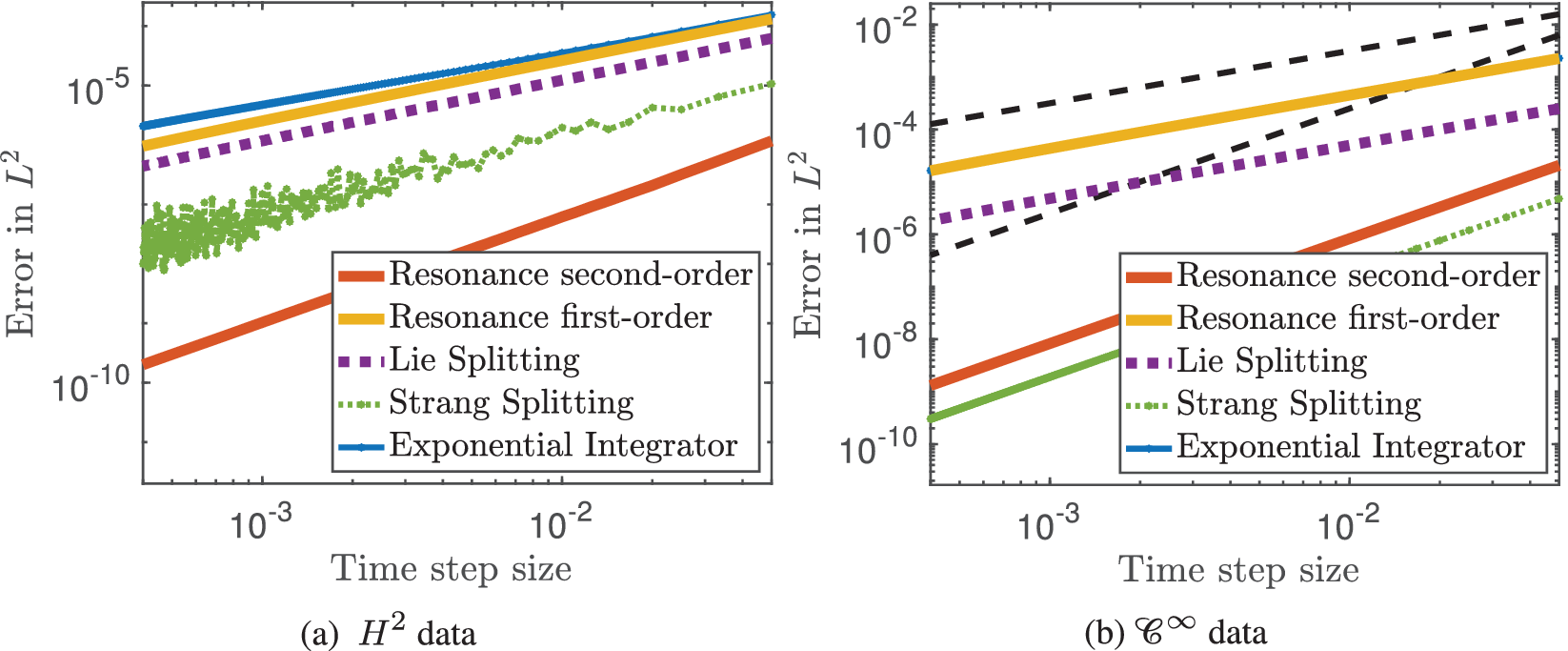
Figure 4 Error versus step size (double logarithmic plot). Comparison of classical and resonance-based schemes for the Schrödinger equation for smooth (right picture) and nonsmooth (left picture) solutions.
Proof
Construction of the schemes. For the second-order scheme we need a local error of order $\mathcal {O}(\tau ^3)$
. Therefore, we need to choose
$\mathcal {O}(\tau ^3)$
. Therefore, we need to choose $r = 1$
in Definition 4.4 and the corresponding trees accordingly. This yields that
$r = 1$
in Definition 4.4 and the corresponding trees accordingly. This yields that
 $$ \begin{align} U_{k}^{n,1}(\tau, v) & = \frac{\Upsilon^{p}( \lambda_k)(v)}{S( \lambda_k)} \Pi^n \left( {\cal D}^1({\cal I}_{({\mathfrak{t}}_1,0)}( \lambda_k)) \right)(\tau)\\ & \quad{}+\sum_{\substack{k_1,k_2,k_3\in {\mathbf{Z}}^d\\-k_1+k_2+k_3 = k}} \frac{\Upsilon^{p}( \lambda_k T_1)(v)}{S(T_1)} \Pi^n \left( {\cal D}^1({\cal I}_{({\mathfrak{t}}_1,0)}( \lambda_k T_1)) \right)(\tau) \notag \\ & \quad{}+\sum_{\substack{k_1,k_2,k_3,k_4,k_5\in {\mathbf{Z}}^d\\-k_1+k_2+k_3 -k_4+k_5= k}} \frac{\Upsilon^{p}( \lambda_k T_2)(v)}{S(T_2)} \Pi^n \left( {\cal D}^1({\cal I}_{({\mathfrak{t}}_1,0)}( \lambda_k T_2)) \right)(\tau) \notag \\ & \quad{}+\sum_{\substack{k_1,k_2,k_3,k_4,k_5\in {\mathbf{Z}}^d\\k_1-k_2-k_3 +k_4+k_5= k}} \frac{\Upsilon^{p}( \lambda_k T_3)(v)}{S(T_3)} \Pi^n \left( {\cal D}^1({\cal I}_{({\mathfrak{t}}_1,0)}( \lambda_k T_3)) \right)(\tau)\notag\end{align} $$
with $T_1$
defined in (126) and
$T_1$
defined in (126) and

In symbolic notation one gets
 $$ \begin{align} \begin{split} & T_2 = {\cal I}_{({\mathfrak{t}}_2,0)} \left( \lambda_k F_2 \right), \quad k = -k_1+k_2+k_3-k_4+k_5 \\ & F_2 = {\cal I}_{({\mathfrak{t}}_1,1)}( \lambda_{k_4}) {\cal I}_{({\mathfrak{t}}_1,0)} \left( \lambda_{-k_1+k_2+k_3} T_1 \right){\cal I}_{({\mathfrak{t}}_1,0)}( \lambda_{k_5}), \\ & T_3 = {\cal I}_{({\mathfrak{t}}_2,0)} \left( \lambda_k F_3 \right), \quad k = k_1-k_2-k_3+k_4+k_5 \\ & F_3 = {\cal I}_{({\mathfrak{t}}_1,0)}( \lambda_{k_4}) \overline{{\cal I}_{({\mathfrak{t}}_1,0)}\left( \lambda_{-k_1+k_2+k_3} T_1 \right)}{\cal I}_{({\mathfrak{t}}_1,0)}( \lambda_{k_5}), \end{split} \end{align} $$
where, thanks to (111),
 $$ \begin{align*} \overline{{\cal I}_{({\mathfrak{t}}_1,0)}\left( \lambda_{-k_1+k_2+k_3} T_1 \right)}\ = {\cal I}_{({\mathfrak{t}}_1,1)}\left( \lambda_{-k_1+k_2+k_3} \overline{T_1} \right). \end{align*} $$
Note that the trees $T_2,T_3$
correspond to the next iterated integrals
$T_2,T_3$
correspond to the next iterated integrals
 $$ \begin{align} \begin{split} {\cal I}_2( v^3,\overline{v}^2, \xi ) & = \int_0^\xi e^{-i \xi_1 \Delta} \left[\left(e^{i \xi_1 \Delta} v\right) \left(e^{-i \xi_1 \Delta} \overline{v}\right) \left( e^{i \xi_1 \Delta} {\cal I}_1( v^2,\overline{v}, \xi_1 ) \right) \right] d\xi_1 \\ {\cal I}_3( v^3,\overline{v}^2, \xi ) & = \int_0^\xi e^{-i \xi_1 \Delta} \left[\left(e^{i \xi_1 \Delta} v\right)^{2} \left( e^{-i \xi_1 \Delta} \overline{{\cal I}_1( v^2,\overline{v}, \xi_1 )} \right) \right] d\xi_1. \end{split} \end{align} $$
The definitions (110) imply that
 $$ \begin{align*} \Upsilon^{p}( \lambda_k T_2)(v) & = 2\Upsilon^{p}\left( {\cal I}_{({\mathfrak{t}}_1,1)}( \lambda_{k_4} ) \right) (v) \Upsilon^{p}\left( {\cal I}_{({\mathfrak{t}}_1,0)}( \lambda_{k} T_1) \right) (v) \Upsilon^{p}\left( {\cal I}_{({\mathfrak{t}}_1,0)}( \lambda_{k_5} ) \right) (v)\\ & = 2\overline{\hat{v}}_{k_4} \left( 2 \overline{\hat{v}}_{k_1}\hat{v}_{k_2}\hat{v}_{k_3}\right) {\hat{v}}_{k_5} \\ \Upsilon^{p}( \lambda_k T_3)(v) & = 2 \Upsilon^{p}\left( {\cal I}_{({\mathfrak{t}}_1,0)}( \lambda_{k_4} ) \right) (v) \Upsilon^{p}\left( \lambda_{k} \overline{T_1} \right)(v)\Upsilon^{p}\left( {\cal I}_{({\mathfrak{t}}_1,0)}( \lambda_{k_5} ) \right) (v)\\ & = 2 \hat v_{k_4}\overline{ \left( 2 \overline{\hat{v}}_{k_1}\hat{v}_{k_2}\hat{v}_{k_3}\right) } \hat v_{k_5} = 2 \hat v_{k_4} \left(2 \hat v_{k_1} \overline{\hat{v}}_{k_2} \overline{\hat{v}}_{k_3}\right) \hat v_{k_5} \end{align*} $$
and by (109) we obtain
 $$ \begin{align*} S(T_2) = 1 \cdot 2 = 2, \quad S(T_3) = 2 \cdot 2 = 4. \end{align*} $$
Next we have to compute $ \Pi ^n \left ( {\cal D}^1({\cal I}_{({\mathfrak {t}}_1,0)}( \lambda _k T_j)) \right )$
for
$ \Pi ^n \left ( {\cal D}^1({\cal I}_{({\mathfrak {t}}_1,0)}( \lambda _k T_j)) \right )$
for $j=1, 2,3$
.
$j=1, 2,3$
.
-
1. Computation of
$ \Pi ^n \left ( {\cal D}^1({\cal I}_{({\mathfrak {t}}_1,0)}( \lambda _k T_1)) \right )$
: Here
$k= - k_1+k_2+k_3$
. Similar to (129), we obtain that (141)where by (130) we have that if
$$ \begin{align} \Pi^n \left( {\cal D}^1({\cal I}_{({\mathfrak{t}}_1,0)}( \lambda_k T_1)) \right)(\tau) = e^{-i \tau k^2} {{\cal K}}^{k,1}_{({\mathfrak{t}}_2,1)} \left( e^{ i \xi (k_1^2- k_2^2-k_3^2)},n\right)(\tau), \end{align} $$
$ n\geq 4$
, If
$$ \begin{align*} {{\cal K}}^{k,1}_{({\mathfrak{t}}_2,1)} \left( e^{ i \xi (k_1^2- k_2^2-k_3^2)},n\right)(\tau) = -i \tau + \left(k^2 + k_1^2 - k_2^2-k_3^2\right) \frac{\tau^2}{2}. \end{align*} $$
$ n < 4 $
, with
$$ \begin{align*} {{\cal K}}^{k,1}_{({\mathfrak{t}}_2,1)} \left( e^{ i \xi (k_1^2- k_2^2-k_3^2)},n\right)(\tau) = -i \Psi_{n,0}^1(\mathcal{L}_{\tiny{\text{dom}}},0)(\tau) -i \frac{g(\tau)-1}{\tau} \Psi_{n,0}^1(\mathcal{L}_{\tiny{\text{dom}}},1)(\tau) , \end{align*} $$
Hence,
$$ \begin{align*} \Psi^{1}_{n,0}\left( {\cal L}_{\tiny{\text{dom}}},\ell \right)(\tau) = \left\{ \begin{array}{l} \displaystyle \int_0^{\tau} \xi^{\ell} f(\xi) d \xi, \, \quad \text{if } 4 - \ell> n \text{ and } n < 4 , \\ \displaystyle\sum_{m \leq 1-\ell} \frac{f^{(m)}(0)}{m!} \int_0^{\tau} \xi^{\ell+m} d \xi, \quad \text{if } 4 - \ell \leq n \text{ and } n < 4. \\ \end{array} \right. \end{align*} $$
(142)where
$$ \begin{align} \begin{split} \Pi^{n=2} \left( {\cal D}^1({\cal I}_{({\mathfrak{t}}_1,0)}( \lambda_k T_1)) \right)(\tau) &=-i \tau e^{-i \tau k^2} \Big( \varphi_1(2i \tau k_1^2) + \left(g(\tau)-1\right) \varphi_2(2i \tau k_1^2) \Big)\\ \Pi^{n= 3} \left( {\cal D}^1({\cal I}_{({\mathfrak{t}}_1,0)}( \lambda_k T_1)) \right)(\tau) & = -i \tau e^{-i \tau k^2} \Big( \varphi_1(2i \tau k_1^2) + \frac{1}{2}\left(g(\tau)-1\right)\Big)\\ \Pi^{n \geq 4} \left( {\cal D}^1({\cal I}_{({\mathfrak{t}}_1,0)}( \lambda_k T_1)) \right)(\tau) & = e^{-i \tau k^2} \Big(-i \tau + \left(k^2 + k_1^2 - k_2^2-k_3^2\right) \frac{\tau^2}{2} \Big) \end{split} \end{align} $$
$g(\tau ) = e^{i \tau (k^2 - k_1^2-k_2^2-k_3^2)}$
and
$\mathcal {L}(k) = \mathcal {L}_{\text {dom}}(k) + \mathcal {L}_{\text {low}}(k)$
.
-
2. Computation of
$ \Pi ^n \left ( {\cal D}^1({\cal I}_{({\mathfrak {t}}_1,0)}( \lambda _k T_2)) \right )$
: Here
$k = -k_1+k_2+k_3-k_4+k_5$
. By (83) and
$ P_{{\mathfrak {t}}_1}(k) = -k^2$
, we have Furthermore, by the mulitiplicativity of
$$ \begin{align*} \Pi^n \left( {\cal D}^1({\cal I}_{({\mathfrak{t}}_1,0)}( \lambda_k T_2)) \right)(\tau) & = e^{-i \tau k^2 } \left( \Pi^n {\cal D}^{1}(T_2)\right)(\tau) = e^{-i \tau k^2 } \left( \Pi^n {\cal I}^1_{({\mathfrak{t}}_2,0)} \left( \lambda_k F_2 \right) \right)(\tau)\\ & = e^{-i \tau k^2 } {{\cal K}}_{({\mathfrak{t}}_2,0)}^{k,1}\left(\Pi^n\left({\cal D}^{0}(F_2)\right),n\right)(\tau). \end{align*} $$
$\Pi ^n$
we obtain with the aid of (129) and (131) where by (132) and the fact that
$$ \begin{align*} \Pi^n\left({\cal D}^{0}(F_2)\right) (\tau)& = \left( \Pi^n {\cal I}^0_{({\mathfrak{t}}_1,1)}( \lambda_{k_4}) \right)(\tau) \left(\Pi^n {\cal I}^0_{({\mathfrak{t}}_1,0)} \left( \lambda_{k}T_1 \right)\right)(\tau) \left(\Pi^n {\cal I}^0_{({\mathfrak{t}}_1,0)}( \lambda_{k_5})\right) (\tau)\\ &= e^{-i \tau k_4^2} e^{-i \tau (-k_1+k_2+k_3)^2} {{\cal K}}^{-k_1+k_2+k_3,0}_{({\mathfrak{t}}_2,0)} \left( e^{ i \xi (k_1^2- k_2^2-k_3^2)},n\right)(\tau) e^{-i \tau k_5^2} \\ &= - i e^{-i \tau (k_4^2+k_5^2)} e^{-i \tau (-k_1+k_2+k_3)^2} \Psi_{n,0}^0 \left(\mathcal{L}_{\tiny{\text{dom}}}, 0\right)(\tau) \end{align*} $$
$n \geq 2$
, we have that Hence,
$$ \begin{align*} \Psi_{n,0}^0 \left(\mathcal{L}_{\tiny{\text{dom}}}, 0\right)(\tau) = \tau. \end{align*} $$
(143)where we used again that
$$ \begin{align} \begin{split} \Pi^n \left( {\cal I}^{1}_{({\mathfrak{t}}_1,0)}( \lambda_k T_2) \right)(\tau) & = -i e^{-i \tau k^2 } {{\cal K}}_{({\mathfrak{t}}_2,0)}^{k,1}\left(\xi e^{-i \xi (k_4^2+k_5^2)} e^{-i \xi (-k_1+k_2+k_3)^2} ,n\right)(\tau)\\ & =- e^{-i \tau k^2 } \frac{\tau^2}{2} \end{split} \end{align} $$
$n \geq 2$
.
-
3. Computation of
$ \Pi ^n \left ( {\cal D}^1({\cal I}_{({\mathfrak {t}}_1,0)}( \lambda _k T_3)) \right )$
: Here
$k = k_1-k_2-k_3+k_4+k_5$
. Similarly, we can show that
$$ \begin{align*} \Pi^n \left( {\cal D}^1({\cal I}_{({\mathfrak{t}}_1,0)}( \lambda_k T_3)) \right)(\tau) & = + e^{-i \tau k^2 } \frac{\tau^2}{2}. \end{align*} $$
Plugging the results from Computations 1–3 into (138) yields that
(144)
$$ \begin{align} U_k^{n,1}(\tau,v) & = e^{-i \tau k^2} \hat v_k\\ & \quad {}-i \tau \sum_{-k_1+k_2+k_3 = k}e^{-i \tau k^2} \frac{1}{\tau} \Pi^{n} \left( {\cal I}^{1}_{({\mathfrak{t}}_1,0)}( \lambda_k T_1) \right) (\tau) \, \overline{\hat{v}}_{k_1} \hat v_{k_2} \hat v_{k_2} \notag\\ & \quad {}- \frac{\tau^2}{2} \sum_{-k_1+k_2+k_3-k_4+k_5 = k} e^{-i \tau k^2}\overline{\hat{v}}_{k_1} \hat v_{k_2} \hat v_{k_2} \overline{\hat{v}}_{k_4} \hat v_{k_5}\notag\end{align} $$


with $\Pi ^{n} \left ( {\cal D}^1({\cal I}_{({\mathfrak {t}}_1,0)}( \lambda _k T_1)) \right )$
given in (142) and we have used that the last two sums in (138) can be merged into one. The Fourier-based resonance schemes (144) can easily be transformed back to physical space yielding the three low-to-high regularity second-order iterative schemes (135)–(137) which depend on the smoothness n of the exact solution.
$\Pi ^{n} \left ( {\cal D}^1({\cal I}_{({\mathfrak {t}}_1,0)}( \lambda _k T_1)) \right )$
given in (142) and we have used that the last two sums in (138) can be merged into one. The Fourier-based resonance schemes (144) can easily be transformed back to physical space yielding the three low-to-high regularity second-order iterative schemes (135)–(137) which depend on the smoothness n of the exact solution.
Local error analysis. It remains to show that the general local error bound given in Theorem 4.8 implies the local error
 $$ \begin{align} \mathcal{O}\left( \tau^3 \nabla^n\right), \quad n = 2,3,4 \end{align} $$
of the schemes (135)–(137). Theorem 4.8 implies that
 $$ \begin{align} U_{k}^{n,1}(\tau,v) - U_{k}^{1}(\tau,v) = \sum_{T\kern-1pt\in\kern0.5pt {\mathcal{T}}_0^{3}(R) } {{\cal O}}\left(\tau^{3} {\cal L}^{1}_{\tiny{\text{low}}}(T,n) \Upsilon^{p}( \lambda_k T)(v) \right) \end{align} $$
where ${\mathcal {T}}_0^3(R) = \{ T_0, T_1, T_2, T_3\}$
with
${\mathcal {T}}_0^3(R) = \{ T_0, T_1, T_2, T_3\}$
with $T_0 = {\mathbf {1}}$
,
$T_0 = {\mathbf {1}}$
, $T_1$
given in (126) and
$T_1$
given in (126) and $T_2, T_3$
defined in (139).
$T_2, T_3$
defined in (139).
-
1) Computation of
${\cal L}^{1}_{\tiny {\text {low}}}(T_0, n)$
and
${\cal L}^{1}_{\tiny {\text {low}}}(T_1, n)$
:By Definition 3.11 and Remark 3.14, we obtain similar to the first-order scheme (here with
$r=1$
) that
$$ \begin{align*} \mathcal{L}^1_{\tiny{\text{low}}}\left(T_0,n\right) = 1, \quad \mathcal{L}^1_{\tiny{\text{low}}}\left(T_1,n\right) = k^{\tiny{\text{max}}(n,2)}= k^{\tiny{\text{max}}(n,2)}. \end{align*} $$
-
2) Computation of
${\cal L}^{1}_{\tiny {\text {low}}}(T_2, n)$
:Next we calculate (using again Definition 3.11 and Remark 3.14) that
(147)with
$$ \begin{align} \mathcal{L}^1_{\tiny{\text{low}}}\left(T_2,n\right) & = \mathcal{L}^1_{\tiny{\text{low}}}\left({\cal I}_{({\mathfrak{t}}_2,0)}( \lambda_k F_2),n\right) = \mathcal{L}^0_{\tiny{\text{low}}}\left(F_2,n\right) + \sum_{j} k^{\bar n_j} \end{align} $$
where
$$ \begin{align*} \bar n_j = \max(n, \deg( \mathscr{F}_{\tiny{\text{low}}} ({\cal I}_{({\mathfrak{t}}_2,0)}( \lambda_{k} F^j_2 ))^{2})) \end{align*} $$
$ \sum _j F_2^j = {\mathcal {M}}_{(1)} \Delta {\cal D}^{r-1} (F_2)$
with
$r=1$
. Hence, we have to calculate
$\Delta {\cal D}^{0} (F_2)$
. By the multiplicativity of the coproduct, its recursive definition (69) and the calculation of
${\cal D}^r(T_1)$
given in (70), we obtain that Hence, as
$$ \begin{align*} \Delta {\cal D}^r (F_2) & =\Delta {\cal I}^r_{({\mathfrak{t}}_1,1)}\left( \lambda_{k_4}\right) \Delta {\cal I}^r_{({\mathfrak{t}}_1,0)}\left( \lambda_{-k_1+k_2+k_3}T_1\right)\Delta {\cal I}^r_{({\mathfrak{t}}_1,0)}\left( \lambda_{k_5}\right)\\ &= \left({\cal I}^r_{({\mathfrak{t}}_1,1)}\left( \lambda_{k_4}\right) \otimes {\mathbf{1}} \right)\left( {\cal I}^{r}_{({\mathfrak{t}}_1,0)}( \lambda_{-k_1+k_2+k_3}\cdot) \otimes {\mathrm{id}} \right) \\& \qquad\Delta {\cal D}^{r}(T_1)) \left({\cal I}^r_{({\mathfrak{t}}_1,0)}\left( \lambda_{k_5}\right) \otimes {\mathbf{1}} \right)\\ & = {\cal D}^r(F_2) \otimes {\mathbf{1}} \\ &\quad{} + {\cal I}^r_{({\mathfrak{t}}_1,1)}\left( \lambda_{k_4}\right) {\cal I}^r_{({\mathfrak{t}}_1,0)}\left( \lambda_{k_5}\right) {\cal I}^{r}_{({\mathfrak{t}}_1,0)}\left(\sum_{m \leq r +1 } \frac{ \lambda_{-k_1+k_2+k_3}^m}{m!} \right) \otimes {\cal D}^{(r,m)}( T_1). \end{align*} $$
$r = 1$
, we obtain Now we are in the position to compute
$$ \begin{align*} \sum_{j=1}^4 F^j_2 = {\cal D}^0(F_2) + \sum_{m \leq r +1 } \frac{1}{m!} {\cal I}^0_{({\mathfrak{t}}_1,1)}\left( \lambda_{k_4}\right) {\cal I}^0_{({\mathfrak{t}}_1,0)}\left( \lambda_{k_5}\right) {\cal I}^{0}_{({\mathfrak{t}}_1,0)}\left( \lambda^{m}_{-k_1+k_2+k_3} \right). \end{align*} $$
$\bar n_1$
: By Definition 2.6 we have (148)where we used that
$$ \begin{align} \mathscr{F}_{\tiny{\text{dom}}}\left({\cal I}_{({\mathfrak{t}}_2,0)}\left( \lambda_k F_2\right)\right)& = {\mathcal{P}}_{\tiny{\text{dom}}}\left( P_{({\mathfrak{t}}_2,0)}(k) +\mathscr{F}_{\tiny{\text{dom}}}(F_2) \right)\\ & = {\mathcal{P}}_{\tiny{\text{dom}}}\left(k^2 +\mathscr{F}_{\tiny{\text{dom}}}( F_2)\right)\notag\end{align} $$
$P_{{\mathfrak {t}}_2}(k) = + k^2$
as well as (46). Furthermore, we have that with
$$ \begin{align*} \mathscr{F}_{\tiny{\text{dom}}}\left(F_2\right)& = \mathscr{F}_{\tiny{\text{dom}}}\left( {\cal I}_{({\mathfrak{t}}_1,1)}( \lambda_{k_4}) \right) +\mathscr{F}_{\tiny{\text{dom}}}\left({\cal I}_{({\mathfrak{t}}_1,0)} \left( \lambda_{-k_1+k_2+k_3} T_1 \right)\right) \\ & \quad{}+\mathscr{F}_{\tiny{\text{dom}}}\left({\cal I}_{({\mathfrak{t}}_1,0)}( \lambda_{k_5})\right) \end{align*} $$
where we used that
$$ \begin{align*} \mathscr{F}_{\tiny{\text{dom}}}\left( {\cal I}_{({\mathfrak{t}}_1,1)}( \lambda_{k_4}) \right) = P_{({\mathfrak{t}}_1,1)}(k_4) +\mathscr{F}_{\tiny{\text{dom}}}({\mathbf{1}}) = - P_{{\mathfrak{t}}_1}(-k_4) = +k_4^2 \end{align*} $$
$P_{{\mathfrak {t}}_1}(k) = - k^2$
as well as (46). Similarly, we obtain that Furthermore, we have that
$$ \begin{align*} \mathscr{F}_{\tiny{\text{dom}}}\left( {\cal I}_{({\mathfrak{t}}_1,0)}( \lambda_{k_5}) \right) = - k_5^2. \end{align*} $$
where we used Example 8. Hence,
$$ \begin{align*} \mathscr{F}_{\tiny{\text{dom}}}\left({\cal I}_{({\mathfrak{t}}_1,0)} \left( \lambda_{-k_1+k_2+k_3} T_1 \right)\right) & = - (-k_1+k_2+k_3)^2 + \mathscr{F}_{\tiny{\text{dom}}}\left(T_1 \right)\\ & = - (-k_1+k_2+k_3)^2 + 2 k_1^2 \end{align*} $$
Plugging this into (148) yields
$$ \begin{align*} \mathscr{F}_{\tiny{\text{dom}}}\left(F_2\right) = - (-k_1+k_2+k_3)^2 + 2 k_1^2 + k_4^2 - k_5^2. \end{align*} $$
Therefore,
$$ \begin{align*} \mathscr{F}_{\tiny{\text{dom}}}\left({\cal I}_{({\mathfrak{t}}_2,0)}\left ( \lambda_k F_2 \right)\right) = {\mathcal{P}}_{\tiny{\text{dom}}}\left(k^2 - (-k_1+k_2+k_3)^2 + 2 k_1^2 + k_4^2 - k_5^2\right). \end{align*} $$
$ \mathscr {F}_{\text {low}}\left ({\cal I}_{({\mathfrak {t}}_2,0)}\left ( \lambda _kF_2\right )\right ) = k$
such that Next we compute
$$ \begin{align*} \overline{n}_1 = \text{max}(n,\text{deg}(k^{2})) = \text{max}(n,2). \end{align*} $$
$\overline {n}_2$
: with
$$ \begin{align*} \mathscr{F}_{\tiny{\text{dom}}}\left({\cal I}_{({\mathfrak{t}}_2,0)}\left ( \lambda_k F_2^2 \right)\right) = {\mathcal{P}}_{\tiny{\text{dom}}}\left(k^2 +\mathscr{F}_{\tiny{\text{dom}}}\left(F_2^2\right)\right) \end{align*} $$
$$ \begin{align*} \mathscr{F}_{\tiny{\text{dom}}}\left(F_2^2\right) & = \mathscr{F}_{\tiny{\text{dom}}}\left( {\cal I}_{({\mathfrak{t}}_1,1)}\left( \lambda_{k_4}\right)\right)+\mathscr{F}_{\tiny{\text{dom}}}\left( {\cal I}_{({\mathfrak{t}}_1,0)}\left( \lambda_{k_5}\right) \right)\\ & \quad + \mathscr{F}_{\tiny{\text{dom}}}\left( {\cal I}_{({\mathfrak{t}}_1,0)}\left( \lambda_{-k_1+k_2+k_3} \right) \right). \end{align*} $$
Note that
Together with the previous computations, we can thus conclude that
$$ \begin{align*} \mathscr{F}_{\tiny{\text{dom}}}\left( {\cal I}_{({\mathfrak{t}}_1,0)}\left({ \lambda_{-k_1+k_2+k_3}^m} \right)\right) & = \mathscr{F}_{\tiny{\text{dom}}}\left( {\cal I}_{({\mathfrak{t}}_1,0)}\left( \lambda_{-k_1+k_2+k_3} \right)\right)\\ & = - (-k_1+k_2+k_3)^2. \end{align*} $$
Therefore,
$$ \begin{align*} \mathscr{F}_{\tiny{\text{dom}}}\left({\cal I}_{({\mathfrak{t}}_2,0)}\left ( \lambda_k F_2^2 \right)\right) = {\mathcal{P}}_{\tiny{\text{dom}}}\left(k^2 - (-k_1+k_2+k_3)^2 + k_4^2 - k_5^2 \right). \end{align*} $$
$ \mathscr {F}_{\text {low}}\left ({\cal I}_{({\mathfrak {t}}_2,0)}\left ( \lambda _k F_2^2 \right )\right ) = k$
and
$$ \begin{align*} \bar n_2 = \text{max}(n,2). \end{align*} $$
Hence,
Furthermore, by Definition 3.11 we have
$$ \begin{align*} \bar n_1 = \bar n_2 = \bar n_3 = \bar n_4 = \text{max}(n,2). \end{align*} $$
Plugging this into (147) yields that
$$ \begin{align*} \mathcal{L}^1_{\tiny{\text{low}}}\left( F_2,n\right) & =\mathcal{L}^1_{\tiny{\text{low}}} \left( {\cal I}_{({\mathfrak{t}}_1,1)}\left( \lambda_{k_4}\right) ,n\right) + \mathcal{L}^1_{\tiny{\text{low}}} \left( {\cal I}_{({\mathfrak{t}}_1,0)}\left( \lambda_{-k_1+k_2+k_3} T_1\right) ,n\right) \\ &\quad{} + \mathcal{L}^1_{\tiny{\text{low}}} \left( {\cal I}_{({\mathfrak{t}}_1,0)}\left( \lambda_{k_5}\right) ,n\right)\\ & = \mathcal{L}^1_{\tiny{\text{low}}}({\mathbf{1}}) + \mathcal{L}^1_{\tiny{\text{low}}}\left(T_1 ,n\right) + \mathcal{L}^1_{\tiny{\text{low}}}({\mathbf{1}}) \\ & = 2 + k^{\tiny{\text{max}}(n,2)}. \end{align*} $$
$$ \begin{align*} \mathcal{L}^1_{\tiny{\text{low}}}\left(T_2,n\right) = \mathcal{O}\left( k^{\tiny{\text{max}}(n,2)}\right). \end{align*} $$
-
3) Computation of
${\cal L}^{1}_{\tiny {\text {low}}}(T_3, n)$
: Similarly, we obtain that
$$ \begin{align*} \mathcal{L}^1_{\tiny{\text{low}}}\left(T_3,n\right) = \mathcal{O}\left( k^{\tiny{\text{max}}(n,2)}\right). \end{align*} $$
Plugging the computations 1–3 into (146) we recover the local error structure (145).


5.2 Korteweg–de Vries
We consider the Korteweg–de Vries (KdV) equation
 $$ \begin{align} \partial_t u + \partial_x^{3} u = \frac12 \partial_x u^2 \end{align} $$
with mild solution given by Duhamel’s formula
 $$ \begin{align*} u(\tau) = e^{-\tau \partial_x^{3}} v + \frac12 e^{-\tau \partial_x^{3}} \int_{0}^{\tau} e^{ \xi \partial_x^{3}} \partial_x u^2(\xi) d\xi. \end{align*} $$
The KdV equation (149) fits into the general framework (1) with
 $$ \begin{align*} \mathcal{L}\left(\nabla, \frac{1}{\varepsilon}\right) = i \partial_x^3, \quad \alpha = 1 \quad \text{and}\quad p(u,\overline{u}) = p(u) = i \frac12 u^2. \end{align*} $$
Here $ {\cal L} = \lbrace {\mathfrak {t}}_1, {\mathfrak {t}}_2 \rbrace $
,
$ {\cal L} = \lbrace {\mathfrak {t}}_1, {\mathfrak {t}}_2 \rbrace $
, $ P_{{\mathfrak {t}}_1} = - \lambda ^3 $
and
$ P_{{\mathfrak {t}}_1} = - \lambda ^3 $
and $ P_{{\mathfrak {t}}_2} = \lambda ^3 $
. Then, we denoted by
$ P_{{\mathfrak {t}}_2} = \lambda ^3 $
. Then, we denoted by
an edge decorated by $ ({\mathfrak {t}}_1,0) $
and by
$ ({\mathfrak {t}}_1,0) $
and by
an edge decorated by $ ({\mathfrak {t}}_2,0) $
. Following the formalism given in [Reference Bruned, Hairer and Zambotti13], one can provide the rules that generate the trees obtained by iterating the Duhamel formulation:
$ ({\mathfrak {t}}_2,0) $
. Following the formalism given in [Reference Bruned, Hairer and Zambotti13], one can provide the rules that generate the trees obtained by iterating the Duhamel formulation:
The general framework (115) derived in Section 4 builds the foundation of the first- and second-order resonance-based schemes presented below for the KdV equation (149). The structure of the schemes depends on the regularity of the solution.
Corollary 5.5. For the KdV equation (149), the general scheme (115) takes at first order the form
 $$ \begin{align} \begin{split} u^{\ell+1} &= e^{-\tau \partial_x^3} u^\ell + \frac16 \left(e^{-\tau\partial_x^3 }\partial_x^{-1} u^\ell\right)^2 - \frac16 e^{-\tau\partial_x^3} \left(\partial_x^{-1} u^\ell\right)^2\end{split} \end{align} $$
with a local error of order $\mathcal {O}\Big ( \tau ^2 \partial _x^2 u \Big )$
and at second order
$\mathcal {O}\Big ( \tau ^2 \partial _x^2 u \Big )$
and at second order
 $$ \begin{align} \begin{split} u^{\ell+1} &= e^{-\tau \partial_x^3} u^\ell + \frac16 \left(e^{-\tau\partial_x^3 }\partial_x^{-1} u^\ell\right)^2 - \frac16 e^{-\tau\partial_x^3} \left(\partial_x^{-1} u^\ell\right)^2\\ &\quad{} +\frac{\tau^2}{4} e^{- \tau \partial_x^3}\Psi\big(i \tau \partial_x^2\big) \Big(\partial_x \Big(u^\ell \partial_x (u^\ell u^\ell)\Big)\Big) \end{split} \end{align} $$
with a local error of order $\mathcal {O}\Big ( \tau ^3 \partial _x^4 u \Big )$
and a suitable filter function
$\mathcal {O}\Big ( \tau ^3 \partial _x^4 u \Big )$
and a suitable filter function $\Psi $
satisfying
$\Psi $
satisfying
 $$ \begin{align*} \Psi= \Psi\left(i \tau \partial_x^2 \right), \quad \Psi(0) = 1, \quad \Vert \tau \Psi \left(i \tau \partial_x^2\right) \partial_x^2 \Vert_r \leq 1. \end{align*} $$
Remark 5.6. Note that the first-order scheme (150) which was originally derived in [Reference Hofmanová and Schratz50] is optimised as the resonance structure factorises in such a way that all frequencies can be integrated exactly (details are given in the proof). This is in general true for equations in one dimension with quadratic nonlinearities up to first order. However, this trick cannot be applied to derive second-order methods. The second-order scheme is new and allows us to improve the local error structure $\mathcal {O}\left ( \tau ^3 \partial _x^5 u \right )$
introduced by the classical Strang splitting scheme [Reference Holden, Lubich and Risebro54]. Due to the stability constraint induced by Burger’s nonlinearity, it is preferable to embed the resonance structure into the numerical discretisation even for smooth solutions. In Figure 5 we numerically observe the favourable error behaviour of the new resonance-based scheme (151) for
$\mathcal {O}\left ( \tau ^3 \partial _x^5 u \right )$
introduced by the classical Strang splitting scheme [Reference Holden, Lubich and Risebro54]. Due to the stability constraint induced by Burger’s nonlinearity, it is preferable to embed the resonance structure into the numerical discretisation even for smooth solutions. In Figure 5 we numerically observe the favourable error behaviour of the new resonance-based scheme (151) for $\mathcal {C}^\infty $
solutions.
$\mathcal {C}^\infty $
solutions.

Figure 5 Error versus step size (double logarithmic plot). Comparison of classical and resonance-based schemes for the KdV equation with smooth data in $\mathcal {C}^\infty $
.
$\mathcal {C}^\infty $
.
Proof
The proof follows the line of argumentation to the analysis for the Schrödinger equation. The construction of the schemes is again based on the general framework (115). Hence, we have to consider for $r = 0,1$
 $$ \begin{align} U_{k}^{n,r}(\tau, v) = \sum_{T\kern-1pt\in\kern0.5pt {\mathcal{T}}^{r+2}_{0}(R)} \frac{\Upsilon^{p}( \lambda_kT)(v)}{S(T)} \Pi^n \left( {\cal D}^r({\cal I}_{({\mathfrak{t}}_1,0)}( \lambda_k T)) \right)(\tau). \end{align} $$
Thereby, for the first-order scheme the trees of interests are

where $T_1$
is associated to the first-order iterated integral
$T_1$
is associated to the first-order iterated integral
 $$ \begin{align*} {\cal I}_1(v^2,s) = \int_{0}^{s} e^{ s_1 \partial_x^{3}} \partial_x (e^{-s_1 \partial_x^{3}}v)^2 ds_1 \end{align*} $$
and in symbolic notation takes the form
 $$ \begin{align*} T_1 = {\cal I}_{({\mathfrak{t}}_2,0)}\left ( \lambda_{k} F_1\right) \quad F_1 = {\cal I}_{({\mathfrak{t}}_1,0)}( \lambda_{k_1}) {\cal I}_{({\mathfrak{t}}_1,0) }( \lambda_{k_2}) \quad \text{with } k = k_1+k_2. \end{align*} $$
For the first-order scheme we set $r=0$
in (161) such that
$r=0$
in (161) such that
 $$ \begin{align} \begin{split} U_{k}^{n,0}(\tau, v) & = \frac{\Upsilon^{p}( \lambda_kT_0 )(v)}{S(T_0)} \Pi^n \left( {\cal D}^0({\cal I}_{({\mathfrak{t}}_1,0)}( \lambda_k T_0)) \right)(\tau)\\ & \quad + \sum_{k = k_1 + k_2} \frac{\Upsilon^{p}( \lambda_kT_1 )(v)}{S(T_1)} \Pi^n \left( {\cal D}^0({\cal I}_{({\mathfrak{t}}_1,0)}( \lambda_k T_1)) \right)(\tau). \end{split} \end{align} $$
For the first term we readily obtain that
 $$ \begin{align*} \frac{\Upsilon^{p}( \lambda_kT_0)(v)}{S(T_0)} \Pi^n \left( {\cal D}^0({\cal I}_{({\mathfrak{t}}_1,0)}( \lambda_k T_0)) \right)(\tau) = e^{-i \tau k^3} \hat{v}_k. \end{align*} $$
It remains to compute the second term. Note that thanks to (83) we have that
 $$ \begin{align} \begin{split} \Pi^n \left( {\cal D}^0({\cal I}_{({\mathfrak{t}}_1,0)}( \lambda_k T_1)) \right)(\tau) &= e^{i \tau P_{{\mathfrak{t}}_1}(k)}\Pi^n ({\cal D}^0(T_1))(\tau) \\ & = e^{-i \tau k^3} \Pi^n ({\cal I}_{({\mathfrak{t}}_2,0)}^0( \lambda_k F_1) )(\tau) \\ & = e^{-i \tau k^3} \mathcal{K}_{({\mathfrak{t}}_2,0)}^{k,0} \left( \Pi^n ({\cal D}^{-1}(F_1))\right)(\tau). \end{split} \end{align} $$
By the product formula we furthermore obtain that
 $$ \begin{align*} \Pi^n ({\cal D}^{-1}(F_1))(\tau)& = \Pi^n \left( {\cal I}^{-1}_{({\mathfrak{t}}_1,0)} ( \lambda_{k_1})\right) (\tau) \Pi^n \left( {\cal I}^{-1}_{({\mathfrak{t}}_1,0)}( \lambda_{k_2})\right) (\tau) \\ & = e^{-i \tau k_1^3} e^{-i \tau k_2^3}. \end{align*} $$
Plugging the above relation into (154) yields that
 $$ \begin{align*} \Pi^n \left( {\cal D}^0({\cal I}_{({\mathfrak{t}}_1,0)}( \lambda_k T_1)) \right)(\tau) = e^{-i \tau k^3} \mathcal{K}_{({\mathfrak{t}}_2,0)}^{k,0} \left( e^{i \xi (-k_1^3 - k_2^3)} \right)(\tau). \end{align*} $$
Next, we observe that
 $$ \begin{align*} P_{({\mathfrak{t}}_2,0)}(k) - k_1^3-k_2^3 = k^3 - k_1^3 - k_2^3 = 3 k_1 k_2 (k_1+k_2) \end{align*} $$
such that
 $$ \begin{align*} \frac{1}{ P_{({\mathfrak{t}}_2,0)}(k) - k_1^3-k_2^3 } \end{align*} $$
can be mapped back to physical space. Therefore, we set
 $$ \begin{align*} \mathcal{L}_{\tiny\text{dom}} = P_{({\mathfrak{t}}_2,0)}(k) - k_1^3-k_2^3 = 3 k_1 k_2 (k_1+k_2) \end{align*} $$
and integrate all frequencies exactly. This implies
 $$ \begin{align*} \Pi^n \left( {\cal D}^0({\cal I}_{({\mathfrak{t}}_1,0)}( \lambda_k T_1)) \right)(\tau) & = e^{-i \tau k^3} \frac{i (k_1+k_2) }{3i k_1 k_2 (k_1+k_2)} \left(e^{i \tau (k^3 - k_1^3 -k_2^3)}-1\right)\\ & =\frac{1 }{3 k_1 k_2 } \left(e^{- i \tau ( k_1^3 + k_2^3)}- e^{-i \tau k^3} \right). \end{align*} $$
Together with (161) this yields the scheme (150).
For the second-order scheme we need to take into account the following trees:

which are associated to the second-order iterated integral
 $$ \begin{align*} {\cal I}_2(v^3,s) = \int_{0}^{s} e^{ s_1 \partial_x^{3}} \partial_x \left( (e^{-s_1 \partial_x^{3}}v) e^{-s_1 \partial_x^{3}} \int_0^{s_1} e^{s_2 \partial_x^{3}}\partial_x (e^{-s_2 \partial_x^{3}}v)^2 ds_2 \right) ds_1. \end{align*} $$
Then one can proceed as in the second-order schemes for the Schrödinger equation. We omit the details here. The local error analysis is then given by Theorem 4.8, noting that $\alpha = 1$
and
$\alpha = 1$
and
 $$ \begin{align*} \mathcal{L}_{\tiny\text{low}}^0(T_1,\cdot) = k^{1+\alpha}, \quad \mathcal{L}_{\tiny\text{low}}^1(T_1,\cdot) = \mathcal{L}_{\tiny\text{low}}^1(T_2,\cdot) = k^{2(1+\alpha)}. \end{align*} $$
5.3 Klein–Gordon
In this section we apply the general framework (115) to the Klein–Gordon equation
 $$ \begin{align} \partial_t^2 z - \Delta z + \frac{1}{\varepsilon^2} z = \vert z\vert^2 z, \quad z(0,x) = \gamma(x),\quad \partial_t z(0,x) = \frac{1}{\varepsilon^2} \delta(x). \end{align} $$
Here we are in particular interested in resolving the highly oscillatory, so-called nonrelativistic structure of the PDE when the speed of light $c = \frac {1}{\varepsilon }$
formally tends to infinity.
$c = \frac {1}{\varepsilon }$
formally tends to infinity.
Via the transformation $u = z - i \varepsilon {\langle \nabla \rangle _{\frac {1}{\varepsilon }}}^{-1} \partial _t z$
we express (155) in its first-order form
$u = z - i \varepsilon {\langle \nabla \rangle _{\frac {1}{\varepsilon }}}^{-1} \partial _t z$
we express (155) in its first-order form
 $$ \begin{align} & i \partial_t u = -\frac{1}{\varepsilon}{\langle \nabla \rangle_{\frac{1}{\varepsilon}}} u + \frac{1}{\varepsilon}{\langle \nabla \rangle_{\frac{1}{\varepsilon}}}^{-1} \textstyle \frac18 (u + \overline{u})^3, \qquad \frac{1}{\varepsilon}{\langle \nabla \rangle_{\frac{1}{\varepsilon}}} = \frac{1}{\varepsilon}\sqrt{\frac{1}{\varepsilon^2}-\Delta}. \end{align} $$
The first-order form (156) casts into the general form (1) with
 $$ \begin{align*} \mathcal{L}\left(\nabla, \frac{1}{\varepsilon}\right) = \frac{1}{\varepsilon}{\langle \nabla \rangle_{\frac{1}{\varepsilon}}}, \quad \alpha = 0 \quad \text{and}\quad p(u,\overline{u}) = \frac{1}{\varepsilon}{\langle \nabla \rangle_{\frac{1}{\varepsilon}}}^{-1} \textstyle \frac18 (u + \overline{u})^3. \end{align*} $$
The leading operator $\mathcal {L}\left (\nabla , \frac {1}{\varepsilon }\right ) $
thereby triggers oscillations of type
$\mathcal {L}\left (\nabla , \frac {1}{\varepsilon }\right ) $
thereby triggers oscillations of type
 $$ \begin{align*} \sum_{\ell \in {\mathbf{Z}} } e^{ i t \ell \frac{1}{\varepsilon^2}}, \end{align*} $$
which can be formally seen by the Taylor series expansion
 $$ \begin{align*}\mathcal{L}\left(\nabla, \frac{1}{\varepsilon}\right) = \frac{1}{\varepsilon} {\langle \nabla \rangle_{\frac{1}{\varepsilon}}} = \frac{1}{\varepsilon^2} - \frac12 \Delta + \mathcal{O}\left(\frac{\Delta^2}{\varepsilon^2}\right). \end{align*} $$
In oder to determine these dominant oscillations, we define the nonoscillatory operators
 $$ \begin{align} & \mathcal{B}_\Delta = \frac{1}{\varepsilon} {\langle \nabla \rangle_{\frac{1}{\varepsilon}}} - \frac{1}{\varepsilon^2}, \qquad \mathcal{B}_\Delta (k) = \frac{1}{\varepsilon^2} \sqrt{1 + \frac{k^2}{\varepsilon^2}} - \frac{1}{\varepsilon^2} \\ & \mathcal{C}_\Delta = \frac{1}{\varepsilon}{\langle \nabla \rangle_{\frac{1}{\varepsilon}}}^{-1}, \qquad \mathcal{C}_\Delta(k) = \frac{1}{\sqrt{1+ \frac{k^2}{\varepsilon^2}}}, \notag \end{align} $$
which both can be uniformly bounded in $\varepsilon $
thanks to the estimates
$\varepsilon $
thanks to the estimates $\Vert \mathcal {B}_\Delta w \Vert \leq \frac 12 \Vert \Delta w\Vert $
,
$\Vert \mathcal {B}_\Delta w \Vert \leq \frac 12 \Vert \Delta w\Vert $
, $\frac {1}{1+x^2} \leq 1$
. The latter motivates us to rewrite the oscillatory equation (156) in the following form:
$\frac {1}{1+x^2} \leq 1$
. The latter motivates us to rewrite the oscillatory equation (156) in the following form:
 $$ \begin{align} & i \partial_t u = - \left( \frac{1}{\varepsilon^2} +\mathcal{B}_\Delta\right) u + \mathcal{C}_\Delta \textstyle \frac18 (u + \overline{u})^3. \end{align} $$
Here $ {\cal L} = \lbrace {\mathfrak {t}}_1, {\mathfrak {t}}_2 \rbrace $
,
$ {\cal L} = \lbrace {\mathfrak {t}}_1, {\mathfrak {t}}_2 \rbrace $
, $ P_{{\mathfrak {t}}_1} = -\left ( \frac {1}{\varepsilon ^2} + \mathcal {B}_\Delta ( \lambda ) \right ) $
and
$ P_{{\mathfrak {t}}_1} = -\left ( \frac {1}{\varepsilon ^2} + \mathcal {B}_\Delta ( \lambda ) \right ) $
and $ P_{{\mathfrak {t}}_2} = \frac {1}{\varepsilon ^2} + \mathcal {B}_\Delta ( \lambda ) $
. Then, we denoted by
$ P_{{\mathfrak {t}}_2} = \frac {1}{\varepsilon ^2} + \mathcal {B}_\Delta ( \lambda ) $
. Then, we denoted by
an edge decorated by $ ({\mathfrak {t}}_1,0) $
, by
$ ({\mathfrak {t}}_1,0) $
, by
an edge decorated by $ ({\mathfrak {t}}_1,1) $
, by
$ ({\mathfrak {t}}_1,1) $
, by
an edge decorated by $ ({\mathfrak {t}}_2,0) $
and by
$ ({\mathfrak {t}}_2,0) $
and by
an edge decorated by $ ({\mathfrak {t}}_2,1) $
. The rules that generate the trees obtained by iterating the Duhamel formulation are given by
$ ({\mathfrak {t}}_2,1) $
. The rules that generate the trees obtained by iterating the Duhamel formulation are given by
The general framework (115) derived in Section 4 builds the foundation of the first-order resonance-based schemes presented below for the Klein–Gordon equation equation (156).
Corollary 5.7. For the Klein–Gordon equation (156) the general scheme (115) takes at first order the form
 $$ \begin{align} u^{\ell+1} & = e^{i \tau \left(\frac{1}{\varepsilon^2} + \mathcal{B}_\Delta\right)} u^\ell - \tau \frac{3i}{8} e^{i \tau \left(\frac{1}{\varepsilon^2} + \mathcal{B}_\Delta\right)}\mathcal{C}_\Delta \vert u^\ell\vert^2 u^\ell \\ &\quad{} - \tau \frac{i}{8} e^{i \tau \left(\frac{1}{\varepsilon^2} + \mathcal{B}_\Delta\right)} \mathcal{C}_\Delta \Big( \varphi_1\left(2i \frac{1}{\varepsilon^2} \tau\right) \left(u^\ell \right)^3+ 3 \varphi_1\left(-2i \frac{1}{\varepsilon^2} \tau\right) \left \vert u^\ell\right\vert{}^2 u^\ell \notag \\ &\quad{} + \varphi_1\left(-4 i \frac{1}{\varepsilon^2} \tau\right) \left(\overline{u^\ell}\right)^3\Big) \notag \end{align} $$
with a local error $\mathcal {O}\left ( \tau ^2 \Delta u\right )$
and the filter function
$\mathcal {O}\left ( \tau ^2 \Delta u\right )$
and the filter function $\varphi _1(\sigma ) = \frac {e^\sigma -1}{\sigma }$
.
$\varphi _1(\sigma ) = \frac {e^\sigma -1}{\sigma }$
.
If we allow step size restrictions $\tau = \tau \left (\frac {1}{\varepsilon ^2}\right )$
, the general scheme (115) takes the simplified form
$\tau = \tau \left (\frac {1}{\varepsilon ^2}\right )$
, the general scheme (115) takes the simplified form
 $$ \begin{align} u^{\ell+1} = e^{i \tau \left(\frac{1}{\varepsilon^2} + \mathcal{B}_\Delta\right)} u^\ell - \tau \frac{i}{8} e^{i \tau \left(\frac{1}{\varepsilon^2} + \mathcal{B}_\Delta\right)} \mathcal{C}_\Delta \left(u^\ell + \overline{u^\ell}\right)^3 \end{align} $$
with a local error of order $ \mathcal {O}\left ( \frac {\tau ^2}{\varepsilon ^{2}} u \right ) + \mathcal {O}(\tau ^2 \Delta u )$
.
$ \mathcal {O}\left ( \frac {\tau ^2}{\varepsilon ^{2}} u \right ) + \mathcal {O}(\tau ^2 \Delta u )$
.
Remark 5.8. With the general framework we recover at first order exactly the resonance-based first-order scheme (159) derived in [Reference Baumstark, Faou and Schratz4]. If we allow for step size restrictions, we recover a classical approximation of the classical local error structure $\mathcal {O}\left ( \frac {\tau ^2}{\varepsilon ^2}\right )$
introduced by classical Strang splitting or Gautschi-type schemes ([Reference Bao and Dong2]).
$\mathcal {O}\left ( \frac {\tau ^2}{\varepsilon ^2}\right )$
introduced by classical Strang splitting or Gautschi-type schemes ([Reference Bao and Dong2]).
Proof
From the general framework (115) (with $r=0$
) we obtain that
$r=0$
) we obtain that
 $$ \begin{align} U_{k}^{n,0}(\tau, v) = \sum_{T\kern-1pt\in\kern0.5pt {\mathcal{T}}^{2}_{0}(R)} \frac{\Upsilon^{p}( \lambda_kT)(v)}{S(T)} \Pi^n \left( {\cal D}^0({\cal I}_{({\mathfrak{t}}_1,0)}( \lambda_k T)) \right)(\tau) \end{align} $$
with

Let us carry out the computation for the tree $T_1$
which in symbolic notation takes the form
$T_1$
which in symbolic notation takes the form
 $$ \begin{align*} T_1 & = {\cal I}_{({\mathfrak{t}}_2,0)} ( \lambda_k F_1), \quad k = k_1+k_2+k_3 \\ F_1 & = {\cal I}_{({\mathfrak{t}}_1,0)} ( \lambda_{k_1}) {\cal I}_{({\mathfrak{t}}_1,0)}( \lambda_{k_2}) {\cal I}_{({\mathfrak{t}}_1,0)} ( \lambda_{k_3}). \end{align*} $$
Thanks to (83) and the fact that $P_{({\mathfrak {t}}_1,0)}\left (k,\frac {1}{\varepsilon ^2}\right )= \frac {1}{\varepsilon ^2} + \mathcal {B}_\Delta (k)$
, we obtain
$P_{({\mathfrak {t}}_1,0)}\left (k,\frac {1}{\varepsilon ^2}\right )= \frac {1}{\varepsilon ^2} + \mathcal {B}_\Delta (k)$
, we obtain
 $$ \begin{align*} \Pi^n \left( {\cal D}^r({\cal I}_{({\mathfrak{t}}_1,0)}( \lambda_k T_1)) \right)(\tau) & = e^{i \tau P_{({\mathfrak{t}}_1,0)}(k,\frac{1}{\varepsilon})} (\Pi^n {\cal D}^0 (T_1))(\tau) \\& = e^{i \tau \left( \frac{1}{\varepsilon^2} + \mathcal{B}_\Delta(k)\right ) } (\Pi^n {\cal I}^0_{({\mathfrak{t}}_2,0)} ( \lambda_k F_1))(\tau) \\& = e^{i \tau \left( \frac{1}{\varepsilon^2} + \mathcal{B}_\Delta(k)\right ) } \mathcal{K}_{({\mathfrak{t}}_2,0)}^{k,0}\left( \Pi^n {\cal D}^{-1}(F_1) \right)(\tau). \end{align*} $$
By the product rule, we furthermore have that
 $$ \begin{align*} \Pi^n {\cal D}^{-1}(F_1)(\xi) & = \left( \Pi^n {\cal I}^{-1}_{(t_1,0)} \lambda_{k_1}\right)(\xi) \left( \Pi^n {\cal I}^{-1}_{(t_1,0)} \lambda_{k_2}\right)(\xi) \left( \Pi^n {\cal I}^{-1}_{(t_1,0)} \lambda_{k_3} \right)(\xi) \\& = e^{i \xi \left(3 \frac{1}{\varepsilon^2} + \mathcal{B}_\Delta(k_1)+ \mathcal{B}_\Delta(k_2)+ \mathcal{B}_\Delta(k_3)\right ) } \end{align*} $$
such that
 $$ \begin{align} &\Pi^n \left( {\cal D}^0({\cal I}_{({\mathfrak{t}}_1,0)}( \lambda_k T_1)) \right)(\tau)\\ & = e^{i \tau \left( \frac{1}{\varepsilon^2} + \mathcal{B}_\Delta(k)\right ) } \mathcal{K}_{({\mathfrak{t}}_2,0)}^{k,0}\left( e^{i \xi \left(3 \frac{1}{\varepsilon^2} + \mathcal{B}_\Delta(k_1)+ \mathcal{B}_\Delta(k_2)+ \mathcal{B}_\Delta(k_3)\right ) } \right)(\tau). \notag\end{align} $$
Definition 3.1 together with Remark 2.7 and the observation $ P_{({\mathfrak {t}}_2,0)}\left (k,\frac {1}{\varepsilon ^2}\right ) = - \left ( \frac {1}{\varepsilon ^2} + \mathcal {B}_\Delta (k) \right ) $
imply that
$ P_{({\mathfrak {t}}_2,0)}\left (k,\frac {1}{\varepsilon ^2}\right ) = - \left ( \frac {1}{\varepsilon ^2} + \mathcal {B}_\Delta (k) \right ) $
imply that
 $$ \begin{align} \mathcal{L}_{\tiny \text{dom}} & = \mathcal{P} _{\tiny \text{dom}} \left(P_{({\mathfrak{t}}_2,0)}\left(k,\frac{1}{\varepsilon^2}\right) + P \right)\\ & = \mathcal{P} _{\tiny \text{dom}} \left( 2 \frac{1}{\varepsilon^2} - \mathcal{B}_\Delta(k) + \mathcal{B}_\Delta(k_1)+ \mathcal{B}_\Delta(k_2)+ \mathcal{B}_\Delta(k_3 ) \right) = 2 \frac{1}{\varepsilon^2} .\notag \end{align} $$
Hence,
 $$ \begin{align*} \mathcal{K}_{({\mathfrak{t}}_2,0)}^{k,0}\left( e^{i \xi \left(3 \frac{1}{\varepsilon^2} + \mathcal{B}_\Delta(k_1)+ \mathcal{B}_\Delta(k_2)+ \mathcal{B}_\Delta(k_3)\right ) } \right)(\tau) = -i \frac{1}{8} \mathcal{C}_\Delta(k) \frac{e^{2 i \tau \frac{1}{\varepsilon^2}} -1}{2 i \frac{1}{\varepsilon^2}}. \end{align*} $$
Plugging this into (162) yields that
 $$ \begin{align*} \Pi^n \left( {\cal D}^0({\cal I}_{({\mathfrak{t}}_1,0)}( \lambda_k T_1)) \right)(\tau) = - i \tau \frac{1}{8} \mathcal{C}_\Delta(k) \varphi_1\left(2 i \tau \frac{1}{\varepsilon^2}\right) e^{i \tau \left( \frac{1}{\varepsilon^2} + \mathcal{B}_\Delta(k)\right ) }. \end{align*} $$
Together with the observation that
 $$ \begin{align*} \frac{\Upsilon^{p}( \lambda_kT_1)(v)}{S(T_1)} = \hat{v}_{k_1} \hat v_{k_2} \hat v_{k_3} \end{align*} $$
we obtain for the first tree $T_1$
in Fourier space that
$T_1$
in Fourier space that
 $$ \begin{align*} \frac{\Upsilon^{p}( \lambda_kT)(v)}{S(T)} & \Pi^n \left( {\cal D}^0({\cal I}_{({\mathfrak{t}}_1,0)}( \lambda_k T_1)) \right)(\tau) \\ & = - i\tau \frac{1}{8} \mathcal{C}_\Delta(k) \hat{v}_{k_1} \hat v_{k_2} \hat v_{k_3} \varphi_1\left(2 i \tau \frac{1}{\varepsilon^2}\right) e^{i \tau \left( \frac{1}{\varepsilon^2} + \mathcal{B}_\Delta(k)\right ) }. \end{align*} $$
In physical space, the latter takes the form
 $$ \begin{align} &\mathcal{F}^{-1} \left(\frac{\Upsilon^{p}( \lambda_kT)(v)}{S(T)} \Pi^n \left( {\cal D}^0({\cal I}_{({\mathfrak{t}}_1,0)}( \lambda_k T_1)) \right)(\tau) \right)\\ &\quad = -i \frac{1}{8} \tau e^{i \tau \left( \frac{1}{\varepsilon^2} + \mathcal{B}_\Delta \right ) } \mathcal{C}_\Delta\varphi_1\left(2 i \tau \frac{1}{\varepsilon^2}\right) v^3\notag\end{align} $$
with $ \mathcal {B}_\Delta $
and
$ \mathcal {B}_\Delta $
and $ \mathcal {C}_\Delta $
defined in (157). The term (164) is exactly the third term (corresponding to
$ \mathcal {C}_\Delta $
defined in (157). The term (164) is exactly the third term (corresponding to $(u^\ell )^3$
) in the first-order scheme (159). The other terms in the scheme can be computed in a similar way with the aid of the trees
$(u^\ell )^3$
) in the first-order scheme (159). The other terms in the scheme can be computed in a similar way with the aid of the trees $T_j$
,
$T_j$
, $j = 1,2,3,4$
. The local error is then given by Theorem 4.8. For instance, the local error introduced by the approximation of
$j = 1,2,3,4$
. The local error is then given by Theorem 4.8. For instance, the local error introduced by the approximation of $T_1$
reads
$T_1$
reads
 $$ \begin{align*} \mathcal{O}\left(\tau^2 \left(- \mathcal{B}_\Delta(k) + \mathcal{B}_\Delta(k_1)+ \mathcal{B}_\Delta(k_2)+ \mathcal{B}_\Delta(k_3 )\right) \hat v_{k_1} \hat v_{k_2} \hat v_{k_3}\right) = \mathcal{O}(\tau^2 \Delta v^3). \end{align*} $$
The other approximations obey a similar error structure.
The simplified scheme (160), on the other hand, is constructed by carrying out a Taylor series expansion of the full operator $\mathcal {L}_{\tiny \text {dom}} + \mathcal {L}_{\tiny \text {low}} $
. For instance, when calculating
$\mathcal {L}_{\tiny \text {dom}} + \mathcal {L}_{\tiny \text {low}} $
. For instance, when calculating $\mathcal {K}$
, instead of integrating the dominant part (163) for the first tree
$\mathcal {K}$
, instead of integrating the dominant part (163) for the first tree $T_1$
exactly, we Taylor expand the full operator
$T_1$
exactly, we Taylor expand the full operator
 $$ \begin{align*} P_{({\mathfrak{t}}_2,0)}\left(k,\frac{1}{\varepsilon^2}\right) + P = 2 \frac{1}{\varepsilon^2} - \mathcal{B}_\Delta(k) + \mathcal{B}_\Delta(k_1)+ \mathcal{B}_\Delta(k_2)+ \mathcal{B}_\Delta(k_3 ). \end{align*} $$
This implies a local error structure of type
 $$ \begin{align*} \mathcal{O}\left( \frac{\tau^2}{\varepsilon^{2}} u \right) + \mathcal{O}(\tau^2 \Delta u ). \end{align*} $$
We omit further details here.
Remark 5.9. Our framework (115) allows us to also derive second- and higher-order schemes for the Klein–Gordon equation (156). The trees have the same shape as for the cubic Schrödinger equation (119), but many more trees $T\in {\mathcal{T}}^{3}_{0}(R)$
are needed for the description. With our framework we can, in particular, recover the first- and second-order uniformly accurate method proposed in [Reference Baumstark, Faou and Schratz4].
$T\in {\mathcal{T}}^{3}_{0}(R)$
are needed for the description. With our framework we can, in particular, recover the first- and second-order uniformly accurate method proposed in [Reference Baumstark, Faou and Schratz4].
5.4 Numerical experiments
We underline the favourable error behaviour of the new resonance-based schemes compared to classical approximation techniques in case of nonsmooth solutions. We choose $M=2^{8}$
spatial grid points and carry out the simulations up to
$M=2^{8}$
spatial grid points and carry out the simulations up to $T = 0.1$
.
$T = 0.1$
.
Example 21 (Schrödinger). In Figure 4 we compare the convergence of the new resonance-based approach with classical splitting and exponential integration schemes in case of the Schrödinger equation (119) with smooth and nonsmooth solutions. The numerical experiments underline the favourable error behaviour of the resonance-based schemes presented in Corollary 5.3 in case of nonsmooth solutions. While the second-order Strang splitting faces high oscillations in the error causing severe order reduction, the second-order resonance-based scheme maintains its second-order convergence for less regular solutions.
Example 22 (Kortweg–de Vries). Figure 5 underlines the preferable choice of embedding the resonance structure into the numerical discretisation even for smooth solutions of the KdV equation (149). While the second-order classical exponential integrator suffers from spikes in the error when hitting certain (resonant) time steps, the second-order resonance-based scheme presented in Corollary 5.5 allows for full-order convergence without any oscillations.
Acknowledgements
We thank the anonymous referee for her/his extremely valuable remarks. First discussions on this work were initiated while the authors participated in the workshop ‘Algebraic and geometric aspects of numerical methods for differential equations’ held at the Institut Mittag-Leffler in July 2018. The authors thank the organisers of this workshop for putting together a stimulating program bringing different communities together and the members of the institute for providing a friendly working atmosphere. This research was supported by grants from the European Research Council (ERC) under the European Union’s Horizon 2020 research and innovation programme (grant agreement No. 850941).
Conflict of Interest
None.


 Open access