


Impact Statement
Waves similar to those observed at the beach exist throughout the ocean interior and are induced by tides, winds, currents, eddies, and other processes. Similar to beach waves, internal waves can also roll up and break. Widespread internal-wave breaking helps drive the ocean circulation by upwelling the densest waters that form in polar regions and sink to the ocean abyss. They also play an important role in transport and storage of heat, carbon and nutrients. In this work, we show how well-understood physical understanding can be used in conjunction with statistics of observed ocean turbulence to improve our understanding of the impact of small-scale mixing on the global ocean, and thereby on the climate system.
1. Introduction
Turbulence induced by breaking density overturns in the ocean interior, such as those induced by internal waves or boundary layer turbulence, plays a key role in regulating the global ocean circulation and budgets of climatically important tracers such as heat, carbon and nutrients (Reference Garabato and MeredithGarabato & Meredith, 2022; Reference Talley, Feely, Sloyan, Wanninkhof, Baringer, Bullister and ZhangTalley et al., 2016; Reference Whalen, De Lavergne, Naveira Garabato, Klymak, Mackinnon and SheenWhalen et al., 2020). Such turbulence is primarily excited at the bottom of the ocean through interaction of tides, currents and eddies with bottom topography and at the surface through the wind stress acting on the sea-surface (Reference AlfordAlford, 2020; Reference Garabato and MeredithGarabato & Meredith, 2022; Reference Garrett and KunzeGarrett & Kunze, 2007; Reference LeggLegg, 2021; Reference Nikurashin and FerrariNikurashin & Ferrari, 2013). As an example, Figure 1 shows an observationally sampled abyssal high mixing zone, the Samoan Passage, where northward flow of Antarctic Bottom Waters through a constriction generates strong turbulence through a generation of wave-induced and hydraulically controlled density overturns (Reference Alford, Girton, Voet, Carter, Mickett and KlymakAlford et al., 2013; Reference Carter, Voet, Alford, Girton, Mickett, Klymak and TanCarter et al., 2019). Figure 1b highlights the intermittency of turbulence, which renders it difficult to sample sufficiently to allow for accurate quantification of properties of interest such as turbulent mixing. Thus, sampling poses a monumental challenge to connecting our understanding of the physics of turbulence, which occur on scales  $\mathcal {O}(10^{-3}\unicode{x2013}10^{-1})$ m, to the larger scale regional and global implications, which are relevant on scales $\mathcal {O}(10^6\unicode{x2013}10^7)$ m. In this sense, this problem is analogous to cloud physics: both involve micro-physics with leading order global impacts, both occur on scales much smaller than typical climate model resolutions and thus need to be parametrized, and both have been notoriously difficult to parametrize and contribute significantly to inaccuracies in model solutions. In this paper, we provide a novel methodology, based on recent progress in our understanding of the microphysics of mixing (Reference Mashayek, Caulfield and AlfordMashayek, Caulfield, & Alford, 2021, hereafter Reference Mashayek, Caulfield and AlfordMCA21) and statistics of wave-induced turbulence (Reference Cael and MashayekCael & Mashayek, 2021, hereafter Reference Cael and MashayekCM21), to connect the physics of small-scale turbulent mixing to large-scale dynamics. While we make specific choices with regard to the physical parametrization of mixing and statistical distributions of ocean turbulence, our choices may reasonably be thought of as placeholders, based on the best we have today. The machinery to which we refer as a ‘recipe’, however, is a broader framework, the components of which can improve over time, for linking physics and statistics to represent small-scale mixing in ocean/climate models.

Figure 1. (a) Bottom water temperature in the Samoan Passage, a chokepoint of abyssal ocean circulation. (b) Turbulence in the passage: northward velocity (colours), potential temperature (black contours), and dissipation rate measured by a turbulence microstructure profiler (shaded black profiles) and inferred from Thorpe scales (blue profiles). Panels (a,b) are from Reference Alford, Girton, Voet, Carter, Mickett and KlymakAlford et al. (2013). (c) Evolution of the overturn scale,  $L_T$, and upper turbulence bound, $L_O$, as well as the viscous dissipation scale,
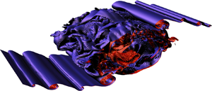
  $L_K$, for an archetypal mixing process in the form of a shear instability of Kelvin Helmholtz type (Reference Mashayek, Caulfield and PeltierMashayek, Caulfield, & Peltier, 2013). The insets show the turbulence breakdown of the wave by showing the spanwise (out of the page) vorticity in grey and counter-rotating streamwise (along flow) vorticity iso-surfaces in green and purple, illustrating the hydrodynamic instabilities that facilitate a wave breakdown (Reference Mashayek and PeltierMashayek & Peltier, 2012a, Reference Mashayek and Peltier2012b). Such instabilities create a turbulence cascade that transfers energy from the energy-containing scale ( $L_T$) to the scales where molecular dissipation erodes momentum ( $L_K$).
The paper is organized as follows. In § 2, we review the physics of small-scale turbulent mixing. In § 3, we provide an overview of the statistics of the observed ocean turbulence and argue that the chronic undersampling of turbulence highlights the inevitability of a statistical approach. In § 4.1, we introduce a recipe that can put the physics and statistics together to infer  $\varGamma _B$. In § 5, we showcase the application of the methodology to an ocean basin. We finish by discussions of the results and their implications in § 7.
2. Physics of wave-induced turbulence
Our understanding of the physics of wave-induced density stratified turbulent mixing has progressed significantly over the past few decades (Reference CaulfieldCaulfield, 2021; Reference Ivey, Winters and KoseffIvey, Winters, & Koseff, 2008; Reference Peltier and CaulfieldPeltier & Caulfield, 2003). A key question concerns how the total power available to turbulence,  $\mathcal {P}$, from winds, tides and other sources, is partitioned into (I) mixing, $\mathcal {M}$, defined as a net vertical irreversible buoyancy flux, and (II) dissipation into heat (due to the seawater viscosity), the rate of which is referred to as $\varepsilon$. The turbulent mixing may be approximated by
 \begin{equation} \mathcal{M}\approx\kappa N^2\approx\varGamma\varepsilon,\end{equation}
where  $N^2=-({g}/{\rho _0})\partial _z\rho$ represents the density stratification, $g$ is the gravitational constant and $\rho _0$ is a reference density (Reference OsbornOsborn, 1980) (note that while the caveats associated with this approximation are important (Reference Mashayek, Caulfield and PeltierMashayek et al., 2013; Reference Mashayek and PeltierMashayek & Peltier, 2013), they do not affect the premise or conclusions of this work in any major way). In physical terms, $\mathcal {M}$ represents a net vertical mass flux as turbulence works against gravity to lift denser waters upward. Such turbulence feeds upon the available potential energy (APE) stored in overturns. Upon mixing, a fraction of the APE gets converted into the background potential energy (i.e. the potential energy that the system would acquire if it were allowed to come to rest adiabatically), with the rest dissipating to heat and increasing the internal energy of the system (which leads to an insignificant temperature rise due to the high heat capacity of seawater; Reference Peltier and CaulfieldPeltier & Caulfield, 2003). The turbulent diffusivity, $\kappa$, is an input parameter in climate models to account for the subgrid-scale unresolved turbulent mixing. The turbulent flux coefficient, $\varGamma =\mathcal {M}/\varepsilon$, is often taken to be a constant value of 0.2 for historical reasons and arguably for the lack of a universally accepted parametrization for it. However, it is well known to be highly variable (Reference CaulfieldCaulfield, 2021; Reference Gregg, D'Asaro, Riley and KunzeGregg, D'Asaro, Riley, & Kunze, 2018; Reference Mashayek and PeltierMashayek & Peltier, 2013), with appreciable consequences for ocean circulation (Reference Cimoli, Caulfield, Johnson, Marshall, Mashayek, Naveira Garabato and VicCimoli et al., 2019; Reference de Lavergne, Madec, Le Sommer, Nurser and Naveira Garabatode Lavergne, Madec, Le Sommer, Nurser, & Naveira Garabato, 2015; Reference Mashayek, Salehipour, Bouffard, Caulfield, Ferrari, Nikurashin and SmythMashayek et al., 2017). While $\mathcal {M}$ is often the quantity of interest from a physical perspective, it is difficult to observe directly and is often inferred from $\varepsilon$ (via (2.1)) which itself is inferred from microscale shear (i.e. spatial gradients of velocity) measured by microstructure probes on profiling instruments, gliders or moorings. Thus, accurate quantification of $\varGamma$ is key to inferring ocean mixing from direct observations.
Three basic turbulence scales have proven useful for parametrization of  $\varGamma$ based on observable quantities. To illustrate their relevance, in Figure 1c, we show their evolution over the life cycle of turbulence breakdown of a canonical overturn. The Kolmogorov scale, $L_K=(\nu ^3/\varepsilon )^{1/4}$, represents the scale below which viscous dissipation takes kinetic energy out of the system, the Ozmidov scale, $L_O=(\varepsilon /N^3)^{1/2}$, is the largest (vertical) scale that is not strongly affected by stratification, and the Thorpe scale, $L_T$, is a geometrical scale characteristic of vertical displacement of notional fluid parcels within an overturning turbulent patch (Reference DillonDillon, 1982; Reference Mashayek, Caulfield and PeltierMashayek, Caulfield, & Peltier, 2017; Reference Smyth and MoumSmyth & Moum, 2000) – $\nu$ is the kinematic viscosity of seawater. The figure shows the initial accumulation of available potential energy (APE) from background shear into the primary billow (large $L_T$) followed by the growth of smaller eddies within the main billow upon feeding on its APE source (increase in $L_O$). As turbulence grows, the scale at which energy is taken out of the system, $L_K$, decreases. The phase where $L_O{\sim }L_T$ is the most efficient transfer of energy from the overturn to the smaller scales, and thus is the richest dynamic range, marked by the largest gap between $L_O$ and $L_K$, and thus the most efficient phase of the flow where (an instantaneous) mixing efficiency is defined as $\mathcal {M}/(\mathcal {M}+\varepsilon )=\varGamma /(1+\varGamma )$ (Reference Peltier and CaulfieldPeltier & Caulfield, 2003). Beyond this efficient phase, both $L_T$ and $L_O$ decay, as does the turbulence.
The ratio of  $L_O$ and $L_K$, often expressed as the buoyancy Reynolds number $Re_b=(L_O/L_K)^{4/3}$, has been widely used to quantify $\varGamma$ (Reference Bouffard and BoegmanBouffard & Boegman, 2013; Reference Gregg, D'Asaro, Riley and KunzeGregg et al., 2018; Reference Mashayek, Salehipour, Bouffard, Caulfield, Ferrari, Nikurashin and SmythMashayek et al., 2017; Reference Monismith, Koseff and WhiteMonismith, Koseff, & White, 2018) and also to establish the global scale impacts of variations in $\varGamma$ (Reference Cimoli, Caulfield, Johnson, Marshall, Mashayek, Naveira Garabato and VicCimoli et al., 2019; Reference de Lavergne, Madec, Le Sommer, Nurser and Naveira Garabatode Lavergne et al., 2015; Reference Mashayek, Salehipour, Bouffard, Caulfield, Ferrari, Nikurashin and SmythMashayek et al., 2017). However, some of these efforts, as well as others, have also highlighted the inherent deficiency of $Re_b$ since it only includes instantaneous information on the turbulence scales $L_O$ and $L_K$ while not ‘knowing’ anything about either the energy containing scale $L_T$ (Reference Gargett and MoumGargett & Moum, 1995; Reference GarrettGarrett, 2001; Reference Mashayek, Caulfield and AlfordMashayek et al., 2021; Reference Mashayek and PeltierMashayek & Peltier, 2011; Reference Mater and VenayagamoorthyMater & Venayagamoorthy, 2014) or any time dependence of the flow, although evidence is accumulating that ‘history matters’ in stratified mixing (Reference CaulfieldCaulfield, 2021). An alternate method for inferring mixing (or more accurately inferring $\varepsilon$ from which diffusivity or flux may be inferred), employed when direct inference of $\varepsilon$ is not available, is to assume that $R_{OT}=L_O/L_T$ is a constant (taken to be between 0.6 and 1; Reference DillonDillon, 1982; Reference Ferron, Mercier, Speer, Gargett and PolzinFerron, Mercier, Speer, Gargett, & Polzin, 1998; Reference ThorpeThorpe, 2005) and $\varGamma =0.2$. This method, too, is inherently deficient (although in practice might be the only available option) since it only ‘knows’ about the energy containing scale and not the dissipation scale, and so does not ‘feel’ the width of the dynamic range of the turbulence (the so-called inertial subrange).
Building on an extensive relevant literature, recently, Reference Mashayek, Caulfield and AlfordMCA21 extended earlier scaling relations relating  $R_{OT}$ to $\varGamma$ and proposed a simple parametrization for $\Gamma$, on basic physical grounds, that agreed well with observational data:
 \begin{equation} \varGamma_i = A\frac{R_{OT}^{{-}1}}{1 + R_{OT}^{{1}/{3}}}, \end{equation}
where  $A$ is a constant ranging between $1/2$ and $2/3$. The subscript $i$ in (2.2) emphasizes the applicability of it to individual turbulent patches as opposed to a bulk region, which typically comprises a multitude of turbulence events separated (in time and space) by ‘quiet’ zones. Crucially, this parametrization captures the fundamental time-dependent nature of overturning mixing events, allowing for variation in $R_{OT}$ and hence $\varGamma$ at different stages in the life cycle of a mixing event. Figure 2a, reproduced from Reference Mashayek, Caulfield and AlfordMCA21, shows the agreement with a combination of data from $\sim$50 000 turbulent patches gathered from six different field campaigns that sampled turbulence in different geographical locations around the globe, at different depths and turbulence regimes, and from turbulence induced by different processes (see supplementary material available at https://doi.org/10.1017/flo.2022.16 for a brief description of data). Equation (2.2) reduces to $A/R_{OT}$ in the limit of young turbulence ( $R_{OT}\ll 1)$) and to $A/R_{OT}^{4/3}$ in the limit of (older) decaying turbulence ( $R_{OT}\gg 1)$). While the latter has been suggested by others in the past, as reviewed in Reference Mashayek, Caulfield and AlfordMCA21, the former limit and the transition between the two limits were formulated in Reference Mashayek, Caulfield and AlfordMCA21.

Figure 2. (a) Agreement of (2.2) with  $\sim$50 000 turbulent patches from six different datasets covering a variety of turbulent regimes and processes. The bar plot insets show the histogram of $R_{OT}$ (top axis) and $\varGamma$ for the parametrization (in red) and data (in blue) along the right vertical axis. The value of $A$ is obtained through regression of data to (2.2). Reproduced from Reference Mashayek, Caulfield and AlfordMashayek et al. (2021) – see supplementary materials for a brief description of data. Note that the data plotted here include observations in the Samoan Passage (shown in Figure 1b) and in the Brazil Basin (of relevance to Figures 5–7). (b) Probability density function (PDF) of $R_{OT}=L_O/L_T$ for the same data as in panel (a), compartmentalized in terms of the rate of dissipation of kinetic energy, $\varepsilon$. The bottom/second/third/top quartiles have increasing modes of 0.66/0.78/0.82/0.88, respectively. Note the negative skewness of the log-transformed PDF. (c,d) Temporal fraction of turbulence lifecycle, as well as the ratio of $R_{OT}$ during the turbulent phase of the flow to its mean value over the whole life cycle. Each symbol represents a life-cycle-averaged quantity from a direct numerical simulation (such as the one in Figure 1d) for the corresponding Reynolds and Richardson numbers. All cases in panel (c) are for $Ri=0.12$ while all cases in panel (d) are for $Re=6000$. The turbulent phases of the life cycles are defined as the times when $Re_b>20$ (Reference GibsonGibson, 1991; Reference Smyth and MoumSmyth & Moum, 2000).
A nice feature of (2.2) is that it allows for the two ranges to merge smoothly at  $R_{OT}{\sim }1$. This limit corresponds to efficient mixing when there exists an optimal balance between the stratification and energy available to turbulence. In the young turbulence range, stratification is relatively high and sufficient energy has not yet transferred to turbulence to work against the stratification and mix. So, while $\varGamma _i$ can be very large, it does not imply much mixing: it is large since $\varepsilon$ is very small, not because $\mathcal {M}$ is large. In fact, in the limit of laminar flow, $\varGamma _i \rightarrow \infty$. However, in the decaying phase of turbulence, stratification is somewhat eroded and so $\mathcal {M}$ is weaker as there is less to mix, while $\varepsilon$ is still finite as even an unstratified flow can have significant $\varepsilon$. Thus, in this limit, $\varGamma _0 \rightarrow 0$. It is the $R_{OT}{\sim }1$ limit in which the right balance of stratification and power exists and optimal mixing occurs. Since this intermediate phase appears to lead to ‘optimal’ mixing, neither too hot nor too cold but ‘just right’, Reference Mashayek, Caulfield and AlfordMCA21 referred to this as ‘Goldilocks mixing’.
Here we argue that all three (time-dependent) phases of the turbulence life cycle, importantly including the young turbulence limit, are key to connecting the small-scale physics of mixing to the large-scale ocean dynamics. While the Goldilocks mixing phase is when most of the effective turbulent flux occurs, the young and weakly turbulent patches are important since most of the ocean interior is relatively ‘quiet’ with intermittent bursts of turbulence. We will argue that it is essential to account for the less/non-turbulent regions, whereas historically, parametrizations have primarily focused on energetic turbulence. This will necessitate careful analysis of the statistics of turbulent patches.
We note that while we will employ the Goldilocks paradigm of Reference Mashayek, Caulfield and AlfordMCA21 in the forthcoming recipe, in principle, it can be replaced by alternative parametrizations for  $\varGamma _i$.
3. Statistics of turbulence
3.1 Statistics of patches
Figure 2b shows the histogram of the data used in Figure 2a separated into four quartiles in terms of  $\varepsilon$. The distribution shows that most turbulent patches lie within a factor of 3 of $R_{OT}=1$ and the larger the $\varepsilon$, the closer to 1 the peak of $R_{OT}$ lies. This suggests the majority of turbulent patches are in this phase of optimal or Goldilocks mixing. Such a clustering of data has been widely reported in the past (Reference DillonDillon, 1982; Reference Mashayek, Caulfield and PeltierMashayek et al., 2017; Reference Mater, Venayagamoorthy, Laurent and MoumMater, Venayagamoorthy, Laurent, & Moum, 2015; Reference ThorpeThorpe, 2005) and suggests that out of the three phases of energetic ocean turbulence events, namely ‘young’ growth, intermediate Goldilocks mixing and ‘old’ decay, the intermediate phase spans the larger fraction of the turbulence life cycle. This is shown quantitatively in Figures 2c and 2d where life-cycle-averaged properties are plotted from turbulence life cycle simulations of shear instabilities by Reference Mashayek and PeltierMashayek and Peltier (2013), Reference Mashayek, Caulfield and PeltierMashayek et al. (2013). Figures 2c and 2d, together, show that for sufficiently energetic turbulence, a larger proportion of the turbulence life cycle corresponds to the Goldilocks phase rather than to the growth and decay phases.
The parametrization (2.2) describes individual turbulent patches. A turbulent region within the ocean, such as that shown in Figure 1b, hosts many patches in different stages of their evolution. Reference Mashayek, Caulfield and AlfordMCA21 argued that an appropriate value for a bulk  $\varGamma$ may be constructed for such a region through
 \begin{equation} \varGamma_{B} = \frac{\mathcal{M}_B}{\varepsilon_B}\approx \frac{\displaystyle \sum_{i = 1}^n \varGamma_i \times \varepsilon_i}{\displaystyle \sum_{i = 1}^n \varepsilon_i}, \end{equation}
where  $n$ represents the number of patches in a region of interest and the subscript $B$ denotes ‘Bulk’. For example, typical resolution of climate models is $\mathcal {O}(100\ {\rm km})$ in the horizontal and $\mathcal {O}(100\ {\rm m})$ in the vertical direction. Models that employ a temporally evolving mixing parametrization, employ $\varGamma _B=0.2$ to construct a diffusivity for each grid cell. Of course there is no obvious reason why such a constant should universally hold, and as we shall show, $\varGamma _{B}$ relies on the statistical distribution of patches within the grid cell and their associated $\varGamma _i$ values. By applying (3.1) to four datasets, Reference Mashayek, Caulfield and AlfordMCA21 showed that $\varGamma _B$ can be close to the Goldilocks mixing (i.e. $A/2\approx 1/3$ in (2.2)) when the region of study has the right balance of power and stratification (where $R_{OT}{\sim }1$), thereby comprising mostly Goldilocks mixing patches. However, regions that host a higher percentage of young or weak turbulent patches can have $\varGamma _B {\sim } \mathcal {O}(1)$ since young patches have large $\varGamma _i$ values, as shown in Figure 3 in the limit of small $R_{OT}$ (Young patches have large $\varGamma$ because of small $\varepsilon$ NOT due to large $\mathcal {M}$. Thus, while they do not contribute much to the net turbulent flux $\sum \varGamma _i \varepsilon _i$, they bias $\varGamma _B$ high).

Figure 3. (a) Sampling bias and uncertainty for buoyancy flux (dashed lines),  $\varGamma \times \varepsilon$ (solid lines) and $\varepsilon$ (dotted lines) for a single turbulent event (e.g. Figure 1c). Purple lines indicate the normalized standard deviation and yellow lines indicate the median relative underestimation, each as a function of sample size, estimated from bootstrap resampling a direct numerical simulation (shown in Figure 1c, from Reference Mashayek, Caulfield and PeltierMashayek et al., 2013). For example, relative uncertainty is ${>}100$ % for the time-averaged buoyancy flux of this event with fewer than $\sim$16 samples, and the median time-averaged buoyancy flux estimate with four or fewer samples underestimates the buoyancy flux by a factor of two or more. (b) Sampling bias and uncertainty for the mean $\varepsilon$ sampled from a log-skew-normal distribution with the parameters estimated from the dataset described in the text, discarding $\varepsilon$ values >10 $^{-5}$ m $^2$ s $^{-3}$. The green line indicates the normalized standard deviation and the orange line indicates the median relative underestimation, each as a function of sample size, estimated from bootstrap resampling.
3.2 Statistics of continuous profiles
Bulk mixing therefore depends on the statistics of turbulent patches. However, weakly/non-turbulent waters reside in between intermittent turbulent patches. Recently, Reference Cael and MashayekCM21 showed that  $\varepsilon$ data from over 750 full depth microstructure profiles from 14 field experiments (covering a wide range of depths, geographical locations and turbulence-inducing processes; see Reference Cael and MashayekCM21 for details), are well described by a log-skew-normal distribution (Figure 4a), which has the form
 \begin{equation} f(\varepsilon;\xi,\omega,\alpha) = \frac{2}{\omega \varepsilon}\phi\left(\frac{\log \varepsilon - \xi}{\omega}\right) \varphi\left(\alpha \frac{\log \varepsilon - \xi}{\omega}\right), \end{equation}
where  $f$ is a probability density function and $\phi$ and $\varphi$ respectively are the probability and cumulative density functions (PDF and CDF) of a standard Gaussian random variable. We refer the reader to Reference Cael and MashayekCM21 for details, but here discuss the essential aspects of that paper for the problem at hand. As discussed in Reference Cael and MashayekCM21, the relationship between the log-skewness ( $\theta$) of the distribution and the additional shape parameter $\alpha$ is one-to-one. The parameters ( $\xi,\omega,\alpha$) are related to the log-mean, log-standard deviation and log-skewness ( $\mu,\sigma,\theta$) of a log-skew-normal random variable according to the following equations:
 \begin{equation} \mu = \xi + \sqrt{\frac{2}{{\rm \pi} }}\omega\delta, \end{equation}
where
 \begin{equation} \delta = \frac{\alpha}{\sqrt{1 + \alpha^2}}, \quad \sigma = \omega \sqrt{1-\frac2{\rm \pi} \delta^2}, \quad \left.\theta = (4-{\rm \pi} )\left(\sqrt{\frac2{\rm \pi} }\delta\right)^3 \right/ \left(2\left(1-\frac2{\rm \pi} \delta^2\right)^{3/2}\right). \end{equation}
Figure 4. (a) Reproduced from Reference Cael and MashayekCM21,  $\varepsilon$ data from over 750 full depth microstructure profiles from 14 field experiments (see Reference Cael and MashayekCael and Mashayek (2021) for more details) are excellently characterized by a log-skew-normal distribution. Cumulative distribution functions (CDFs) are shown in the main plot; the upper inset shows the corresponding probability density functions and that of a log-normal distribution (purple line) for comparison; the lower inset shows the difference between the empirical and hypothesized log-skew-normal CDFs. (b) Regression of log $_{10}(L_T)$ against log $_{10}(L_O)$. The middle line captures the central scaling relationship and is estimated via model II regression as described in the text; the outside lines capture the heteroscedasticity of the residuals and is estimated via quartile regression as described in the text. (c) Mean quantities from the dataset in panel (b) (with error bars representing standard deviation), grouped into three categories: (I) energetic turbulence in weak stratification, (II) weak turbulence in strong stratification, and (III) energetic stratified turbulence; see main text for a discussion. (d) Sensitivity of the bulk flux coefficient to the different $L_T$– $L_O$ scaling parameters, perturbed from a baseline $\varGamma _g$ estimated from the combined global dataset described in the text. Larger fluctuations in $L_T$ when $L_O$ is large can increase the bulk flux coefficient, but it asymptotes to a constant value with decreasing fluctuations. Increasing either the scaling exponent or coefficient increases $L_T$ values for large $L_O$, thus increasing the bulk flux coefficient for large $\varepsilon$; decreasing either the scaling exponent or coefficient drives bulk mixing to zero as $R_{OT}\gg 1$ when $\varepsilon$ is large. See supplementary materials for information on data sources.
The log-skew-normal distribution arises from the analogue of the Central Limit Theorem for lognormal variables: that is, the sum of log-normal variables converges to a log-skew-normal distribution (Reference Wu, Li, Husnay, Chakravarthy, Wang and WuWu et al., 2009). For turbulence, the log-skew-normal distribution is thought to arise because the total, measured  $\varepsilon$ results from a combination of multiple and/or not statistically steady turbulence-generating processes (Reference Caldwell and MoumCaldwell & Moum, 1995), which individually and/or instantaneously have log-normally distributed dissipation rates.
3.3 Chronic undersampling: inevitability of a statistical approach to  $\varGamma _B$

The difficulty of sampling intermittent turbulence has long been recognized (Reference Gregg, Seim and PercivalGregg, Seim, & Percival, 1993), but the problem is perhaps even worse than conventionally thought, owing to the even more heavy-tailed nature of a log-skew-normal  $\varepsilon$ distribution than a lognormal one. This presents a severe challenge for constraining the average $\varepsilon$ value for an ocean volume from a limited sample set, since many samples are required to resolve the disproportionately consequential tail. Direct numerical simulations have established that turbulent quantities, such as $\varepsilon$ and $\Gamma$, vary substantially over the lifetime of an overturning event (Reference CaulfieldCaulfield, 2021). This implies that a single measurement, or even a handful of measurements, of such an event can be a poor estimate of its time-integrated properties since they most likely miss the most energetic phase of turbulence for each event. This underscores the need for large measurement sets and a statistical approach to fill in the gaps and accurately estimate bulk turbulent properties. To highlight the sampling issue, in Figure 3, we consider two examples: one based on sampling of an individual turbulence event; and one based on sampling of the collective global dataset discussed in Figure 4a.
Direct numerical simulations, such as that shown in Figure 1c, clearly demonstrate that turbulent quantities such as  $\mathcal {M}$, $\varepsilon$ and $\varGamma$ vary substantially over the lifetime of an overturning event. This implies that a single measurement, or even a handful of measurements, of such an event are highly likely to be a poor estimate of its time-integrated properties. Figure 3a shows the uncertainty and bias associated with random samples of one (other simulations yielded similar results) simulation's history $(Re = 6000, Ri = 0.16)$ for different sample sizes. Uncertainty is quantified by the normalized standard deviation of the sample mean for collections of samples taken at random times along the temporal history of the overturning event. Bias is quantified by the ratio of the median sample mean from these collections of randomly timed samples to the true time-averaged mean of each property. Because all the properties shown are positively skewed quantities, the sample means tend to miss the peak values and thus underestimate the time-averaged value; because these skews are so large, means of different collections of random samples vary by e.g. more than a factor of two for fewer than $\sim$16 measurements. Turbulent measurements are snapshots of events; it is not possible to make tens of measurements of the same turbulent event. These appreciable biases and uncertainties for characterizing individual events thus underscore the importance of the statistics of turbulent properties.
The heavy-tailed nature of the  $\varepsilon$ distribution in Figure 4a presents a similar challenge for constraining the average $\varepsilon$ value for an ocean volume from a limited sample set. Figure 3b shows the same as Figure 3a, but for random samples from a log-skew-normal distribution whose parameters are fit to match the $\varepsilon$ data from the experiments described above ( $\xi = -24.8$, $\omega = 3.91$, $\alpha = 5.89$) using the same procedure as in Reference Cael and MashayekCM21. We discard values above a chosen $\varepsilon _{max}$ threshold of $10^{-5}$ m $^2$ s $^{-3}$; as with any parametrization for the PDF of $\varepsilon$ supported on $(0,\infty )$, the log-skew-normal allows for a non-zero probability density for unmeasurably and/or unphysically large $\varepsilon$ values, which are either too large to be measured by sampling probes and/or yield impossibly large $L_O$ values. Here, $\mathcal {O}(1000)$ samples are needed to make the underestimation bias less than $\sim$10 %, and $\mathcal {O}(100)$ samples are needed to make the standard deviation of sample means less than the true mean (i.e. <100 % relative uncertainty). (Larger/smaller values of $\varepsilon _{max}$ increase/reduce these sample size numbers.) This further underscores the need for large measurement sets and a statistical approach to estimate bulk turbulent properties accurately.
4. A recipe for $\varGamma _B$

Ingredients:  $\varGamma (R_{OT})$ for individual patches + statistics of $L_O$, $L_T$, and $R_{OT}$.
Here, we aim to exploit the log-skew-normality of  $\varepsilon$ and the statistics of $R_{OT}$ to construct a parametrization for $\varGamma _B$ based on the total power and the mean stratification for the region (or the grid cell) for which $\varGamma _B$ is sought. To this end, first we note that $L_O \propto \varepsilon ^{1/2}$ by definition; the former lies within the $R_{OT}$-based $\varGamma$ parametrization in (2.2) and the latter is captured by (3.2) (historically, $\varepsilon$ has often been described as log-normally distributed based on a simple argument from multi-stage subdivisions of an initial flux for three-dimensional homogeneous isotropic turbulence (Reference Gurvich and YaglomGurvich & Yaglom, 1967), but the log-normal distribution has also been long recognized as a quantitatively inaccurate description of measured distributions (Reference Yamazaki and LueckYamazaki & Lueck, 1990)). Because $L_O$ divides $\varepsilon$ by another random variable and then takes a square root of their quotient, this distribution is also preserved for $L_O$ (supplementary material, Figure S1, Table S1; also see below). Here, we pair the parametrizations for the statistical distribution of $\varepsilon$ in (3.2) and $\varGamma _i=f(R_{OT})$ in (2.2) to obtain a parametrization for $\varGamma _B$.
If, as described above,  $\varepsilon _B$ is log-skew-normally distributed because it is the sum of log-normal random variables (call these $\varepsilon _i$), then $L_O$ must also be so distributed. If we pass the $N^3$ to the summed-over $\varepsilon _i$, such that $\varepsilon _B/N^3 = \sum _i (\varepsilon _i/N^3)$, this will introduce a correlation into the $\varepsilon _i/N^3$ being summed over, which does not affect the log-skew-normality of their sum (Reference Hcine and BouallegueHcine & Bouallegue, 2015). For the $\varepsilon _i$, this introduces another variable multiplicative factor and these each should still then be log-normal, so altogether $\sum _i (\varepsilon _i/N^3)$ is still the sum of log-normal random variables. As the skew-normal distribution is insensitive to multiplicative transformations – we may write any skew-normal random variable $s$ as $s = \mu + \sigma (\delta |n_1| + n_2 \sqrt {1 - \delta ^2})$ (Reference PourahmadiPourahmadi, 2007) so multiplying by some factor $m$ just changes $\mu \to m\mu$ and $\sigma \to m\sigma$ – the log-skew-normal must be equivalently insensitive to exponentiation. Thus, if $\varepsilon _B$ is log-skew-normally distributed, then so is $L_O$. We indeed find that all the datasets used here, as well as their aggregate, are well described by a log-skew-normal distribution (Kuiper's statistic $V = 0.021$ for the combined dataset and as well as the median across the individual datasets; supplementary material, Figure S1, Table S1).
In contrast, there is not a clear description of the probability distribution of  $L_T$. While calculating $L_T$ is straightforward conceptually, it involves subjective choices that bias its distribution (Reference Mater, Venayagamoorthy, Laurent and MoumMater et al., 2015). Thus, it is less practical to identify the ‘true’ distribution for $L_T$ from collections of $L_T$ measurements, as is the equivalent identification of an underlying distribution for $\varepsilon$. It has recently been argued that the size of turbulent overturns, which are thought to have a correspondence with $L_T$, should be power-law distributed (Reference Smyth, Nash and MoumSmyth, Nash, & Moum, 2019), but we find little to no evidence of this in the datasets we use here (supplementary material, Table S2). Either $L_T$ is not proportional to patch size in the datasets examined here or the patch sizes in these datasets are not power-law distributed (Reference Clauset, Shalizi and NewmanClauset, Shalizi, & Newman, 2009). The $L_T$ probability distribution for all the datasets used here is unimodal in log-space, such that at least the bulk of the distributions are qualitatively much closer to log-normally distributed than power-law distributed (supplementary material, Figure S1).
Regardless, it is the probability distribution of  $R_{OT} = L_O/L_T$ that is of interest here, for which a parametrization of the probability of $L_T$ is not necessary. Instead, one needs a suitable description of the conditional distribution of $L_T$ for a given $L_O$ value, i.e. $P(L_T | L_O)$. Somewhat surprisingly, we find that the log-skew-normal distribution is again an excellent description of the probability distribution of $R_{OT}$ ( $V = 0.010$ for the combined dataset and the median $V = 0.027$ across the eight individual datasets; supplementary material, Table S1), but that in this case, the log-skewness is negative. The log-skewness of $R_{OT}$ is in fact only positive for the IH18 dataset (skewness $\tilde {\mu }_3 = 0.48$). Thus, the log-skew-normal distribution is, similar to $\varepsilon$ and $L_O$, a satisfactory parametrization of the probability distribution of $R_{OT}$, but by and large with a different sign in log-skewness. The question then becomes how $L_O$ and $L_T$ are related such that the distribution of $R_{OT}$: (i) is log-skew-normal; (ii) has a negative log-skewness and (iii) is peaked at $\mathcal {O}(1)$. In the absence of a theory for the probability distribution of $L_T$, we derive an empirical construction of $P(L_T|L_O)$ that recapitulates the probability distribution of $R_{OT}$ with simulated $L_T$ values. As $L_T$ appears to be approximately log-normally distributed (supplementary material, Figure S1), it is justifiable to base such a construction on a statistical scaling relationship, with multiplicative fluctuations.
The conditions (i–iii) above can occur for  $R_{OT}$ if $L_T$ scales heteroscedastically, i.e. the fluctuations around how $L_T$ scales with $L_O$ are themselves also a function of $L_O$, and the coefficients of the scaling relationship are close to unity. If $L_T {\sim } \zeta L_O^\beta$ with $\zeta \approx 1$ and $\beta \approx 1$, then most values of $L_O/L_T$ will be $\mathcal {O}(1)$. If this scaling relationship is tight when $L_O$ is large (i.e. small fluctuations and low probability of small $L_T$), this will make cases where $L_O/L_T$ is very large unlikely. Conversely, if this scaling relationship is weaker when $L_O$ is small (i.e. larger fluctuations and comparatively higher probability of larger $L_T$), this will make cases where $L_O/L_T$ is very small less unlikely. Together, these heteroscedastic effects can change the sign of the log-skewness.
As both  $L_O$ and $L_T$ are random variables, their scaling relationship can be captured by model II regression; the heteroscedasticity of this relationship can then be captured by quantile regression, which estimates the conditional quantiles of the response variable (Reference Koenker and HallockKoenker & Hallock, 2001), applied to the residuals. First, applying model II regression to the combined and log-transformed $(L_O,L_T)$ dataset (i.e. that used in Figure 2a,b), we find the best-fit scaling for these data to be $L_T = 1.24 L_O^{1.01}$ (see Figure 4b; we use least-squares cubic regression (Reference YorkYork, 1966) but other standard methods such as bisector or major axis yield similar results). Then applying quantile regression to the residuals, we indeed find that the fluctuations in $L_T$ around this scaling relationship increase as $L_O$ decreases. This decrease is characterized by the relationship $r = r_o + r_1 \log _{10} (L_O)$, where $r$ is the amplitude of the residuals around the best-fit scaling, $r_o$ is the residual amplitude when $L_0 = 1$ m and $r_1$ captures how the residuals decrease as $L_O$ increases. We calculate separate relationships for positive and negative residuals, via quantile regression. (We use the 10th and 90th percentiles to compute $r_o$ and $r_1$ but our results are not sensitive to this choice.) We can then recover the joint $(L_O,L_T)$ distribution and hence the $R_{OT}$ distribution by simulating the $L_T$ accordingly for a given $L_O$. The simulated $L_T$ values yield good agreement with the empirical $R_{OT}$ distribution ( $V = 0.028$). We define $L_T = \eta \times 1.24 L_O^{1.01}$, where $\eta$ is a log-normal random variable with $\mu = 0$ and $\sigma \propto L_O$. This results in a conditional distribution for $L_T$ that matches the estimated scaling relationships, and is thus an approximation of the joint distribution of the data shown in Figure 4b.
Physically, this scaling behaviour has an intuitive interpretation (as illustrated in Figure 4c):  $L_T$ scaling with $L_O$ with an exponent close to unity, such that the peak in the probability density function for $R_{OT}$ is $\mathcal {O}(1)$, occurs because for most turbulent overturns, the displacement of fluid parcels in that patch ( $L_T$) will be of the same order of magnitude as the vertical scale that they can be displaced given the background stratification ( $L_O$), as discussed above. If an overturn has a small $L_O$, this could either be because it is a small overturn, meaning it has a similarly small $L_T$, or a young overturn with a larger $L_T$ but still low turbulent dissipation. If $L_O$ is large, however, it likely corresponds to the energetic phase of the flow (i.e. the optimal mixing phase in Figure 1c) and so $L_T$ could be reasonably expected to be similarly large. This asymmetry in the life cycle of turbulent overturns produces this skewed, heteroscedastic scaling in Figure 4b. Figure 4c groups the data in Figure 4b (same as that in Figures 2a and 2b) into the three categories discussed above, and shows that (a) weak stratification cannot yield a high flux coefficient even at high energy levels as there is barely enough to mix, (b) low energy turbulence in the presence of strong stratification can result in a high flux coefficient, but importantly that does not imply a high flux (since flux $\approx \varGamma \varepsilon$); note that in the limit of no turbulence, $\varGamma \rightarrow \infty$ but flux tends to zero, and (c) for energetic stratified turbulence, the flux coefficient is within the conventional range (0.2–0.3). It is only the latter category (c) that corresponds to large effective turbulent flux.
4.1 The recipe
Altogether, these pieces can be assembled into a ‘recipe’ to compute a bulk flux coefficient as follows. To calculate  $\varGamma _B$ for a coarse resolution grid cell of a general circulation model, which is large enough to enclose sufficient statistics, we imagine a total power $\mathcal {P}$ is available for the grid cell (from one or more sources, such as tides, winds, etc.). Then, we follow the iterative procedure below.
(1) Assume an initial value of 0.2 for
$\varGamma _B$ and using $\mathcal {P}=\mathcal {M}_B+\varepsilon _B$, infer an initial value for $\varepsilon _B$; $\mathcal {M}_B$ and $\varepsilon _B$ are the total mixing and dissipation in the cell.(2) Distribute
$\varepsilon _B$ over a log-skew-normal distribution of $\varepsilon$ for individual patches, so then $\varSigma \varepsilon _i=\varepsilon _B$ and individual $\varepsilon _i$ values are random log-skew-normal sample draws.(3) Calculate
$L_O$ for these patches by transforming their $\varepsilon$ values and a specified background stratification into a distribution for $L_O$.(4) Simulate
$L_T$ values corresponding to these $L_O$ values according to the heteroscedastic scaling relationship between $L_O$ and $L_T$.(5) Calculate
$\varGamma$ for these patches based on the $R_{OT}$ parametrization and their simulated $L_O$ and $L_T$ values (with a small background diffusivity added; see below).(6) Calculate
$\mathcal {M}_i$ for individual patches based on their $\varGamma _i$.(7) Sum over
$\mathcal {M}_i$ of all patches to compute $\mathcal {M}_B$.(8) Calculate
$\varGamma _B=\mathcal {M}_B/\varepsilon _B$.(9) Back to step one and iterate until
$\varGamma _B$ converges (usually within a few iterations).


We repeat this procedure many times and take the average of the realizations to account for the stochasticity in the process; in practice, for oceanographically relevant values, the variability between realizations is negligible. In step 5, we also add a small (regularizing) background diffusivity of  $\kappa _{background} = 10^{-6.5}$ m $^2$ s $^{-1}$ to account for the background wave field processes not encapsulated in the $R_{OT}$ parametrization. This value, which is close to the molecular diffusion coefficient of heat in seawater, was chosen according to the inflection point on the probability density function of $\kappa$ from the combined dataset described above, which separates the low tail of the distribution from the bulk of the data (supplementary material, Figure S2). Including this $\kappa _{background}$, mixing for each patch becomes
 \begin{equation} \mathcal{M}_i = \mathcal{M}_{background} + \mathcal{M}_{turbulent} = \varGamma_{i}\varepsilon_i = \kappa_{background} N^2 + \varGamma_{turbulent} \varepsilon_i, \end{equation}
and so the effective total flux coefficient for individual patches may be defined as
 \begin{equation} \varGamma_i = \kappa_{background} N^2/\varepsilon_i + \varGamma_{turbulent}, \end{equation}
where  $\varGamma _{turbulent}$ is from (2.2). The advantage of adding the background mixing is that it allows for $\varGamma$ to tend to large values in the limit of weak turbulence, i.e. when there is not much turbulence due to lack of power and/or overly strong stratification. From a physical perspective, in the limit of laminar flow, $\varGamma \rightarrow \infty$ since $\varepsilon$ vanishes but $\mathcal {M}$ remains finite. For example, note that Figure 2a shows high values of $\varGamma$ for observed weakly turbulent young patches.
Steps 1–5 in the above recipe involve a degree of computational expense that might prove impractical if applied to every grid cell of a coarse resolution climate model at every time step. It is, however, straightforward and computationally cheap to do the calculations a priori for ranges of power and stratification relevant to the oceans, and then employ a simple lookup table in the models. We employ this approach for the purpose of analysis to be discussed in the next section.
5. Regional/global implications
To highlight the importance of  $\varGamma _B$ for the larger scale circulation, we next apply our recipe to the South Atlantic Ocean. This choice is made for four reasons: (I) it is a region of tidal-shear dominance; (II) it is home to the iconic Brazil Basin Tracer Release Experiment (BBTRE), the first deep observation of bottom generated enhanced turbulent mixing (Reference Ledwell, Montgomery, Polzin, Laurent, Schmitt and TooleLedwell et al., 2000; Reference Polzin, Toole, Ledwell and SchmittPolzin, Toole, Ledwell, & Schmitt, 1997; Reference St. Laurent, Toole and SchmittSt. Laurent, Toole, & Schmitt, 2001); (III) there exist three-dimensional tidal power estimates which are constructed on theoretical grounds but have been verified to agree excellently with observations including BBTRE (Reference de Lavergne, Vic, Madec, Roquet, Waterhouse, Whalen and Hibiyade Lavergne et al., 2020) and (IV) the BBTRE data were shown to correspond to small-scale marginally unstable shear-induced turbulence, and hence consistent with the above-mentioned physical and statistical paradigms laid out in Reference Cael and MashayekCM21, Reference Mashayek, Caulfield and AlfordMCA21.
We construct a regional map from the sum of the tidally generated power and the contribution of the wind-induced near-inertial shear. The former, from Reference de Lavergne, Falahat, Madec, Roquet, Nycander and Vicde Lavergne et al. (2019, Reference de Lavergne, Vic, Madec, Roquet, Waterhouse, Whalen and Hibiya2020), estimates the power in the internal tide field generated through the interaction of ocean tides with ocean bathymetry. The latter, constructed based on Reference AlfordAlford (2020), estimates the power in the downward-propagating wind-induced internal wave field. Figure 5a–c shows the combined power plotted on three density layers (shallow, intermediate depth and deep) (neutral density is often used instead of in situ density as it removes the dynamically inconsequential compression of seawater due to increase in pressure with depth. It is also common to deduct 1000 when reporting neutral density, as in Figure 5). The deep layer, as will be shown, corresponds to the peak cross-density (diapycnal) turbulence-induced upwelling that helps sustain the deep branch of the ocean circulation (Reference de Lavergne, Madec, Roquet, Holmes and McDougallde Lavergne, Madec, Roquet, Holmes, & McDougall, 2017). The shallow layer approximately corresponds to the base of the subtropical wind-driven gyres, across which turbulence mixes heat, carbon and nutrients between the upper ocean and the deep ocean (Reference TalleyTalley, 2011). The patterns on the shallow layer reflect the seasonal atmospheric storm patterns at the surface and the rough topography at the bottom (from which internal tides radiate upwards). The patterns on the deep layer primarily represent the tidally generated turbulence, with little contribution from the surface generated downward propagating waves. The intermediate layer ‘feels’ both top and bottom generated wave fields.

Figure 5. (a–c) Power in the internal wave field in the South Atlantic basin, induced by tides and winds, that is available for mixing and dissipation, plotted on various density levels. (d–f)  $\varGamma _B$ normalized by $\varGamma ^*=A/2$ based on (2.2), plotted on the same density levels as in panels (a–c). Since $\kappa \approx \varGamma _B \varepsilon /N^2$ and the turbulent flux is $\mathcal {M} \approx \kappa N^2$, $\varGamma _B/0.2$ is equal to ratios of $K$ and $\mathcal {M}$ based on $\varGamma _B$ calculated using our recipe to their values when 0.2 is used.
The power maps, together with climatological hydrographic information (i.e.  $N^2$) from the World Ocean Circulation Experiment (WOCE; see Reference Gouretski and KoltermannGouretski & Koltermann, 2004), enable us to calculate $\varGamma _B$ on the WOCE grid on which the power maps in Figure 5 are constructed (following Reference de Lavergne, Vic, Madec, Roquet, Waterhouse, Whalen and Hibiyade Lavergne et al., 2020). The resolution of the grid is half a degree in the horizontal ( $\sim$50 km) and $\sim$110 m in the vertical. Applying our recipe to each grid cell with its local power and density stratification, we obtain the maps of $\varGamma _B$ shown in Figure 5d–f , normalized by 0.2. Since the bulk turbulent diffusivity for each grid cell may be approximated as $\kappa \approx \varGamma _B N^2/\varepsilon _B$ and the associated buoyancy flux is defined as $\mathcal {M}_B\approx \kappa N^2$, the ratio $\varGamma _B/0.2$ is exactly equal to the ratios of $\kappa$ and $\mathcal {M}$ calculated based on our recipe to their values when calculated using $\varGamma _B=0.2$. Thus, Figure 5d–f represents all three ratios and collectively show significant spatial variations to $\varGamma _B$. For example, for flux of a given quantity $\mathcal {C}$ between the surface ocean and the deep ocean (where $\mathcal {C}$ can be heat, carbon or nutrients for example), Figure 5d implies that the flux $\kappa \mathcal {C}$ can be overestimated or underestimated by more than 200 % if $\varGamma _B= 0.2$ is used.
In the deep ocean, turbulent mixing leads to the irreversible transformation of water masses into lighter/denser waters (i.e. upwelling/downwelling), which facilitates a net upwelling of the dense abyssal waters, thereby closure of the deep branch of ocean meridional circulation (Reference Ferrari, Mashayek, McDougall, Nikurashin and CampinFerrari, Mashayek, McDougall, Nikurashin, & Campin, 2016; Reference de Lavergne, Madec, Le Sommer, Nurser and Naveira Garabatode Lavergne, Madec, Le Sommer, Nurser, & Naveira Garabato, 2016; Reference Mashayek, Ferrari, Nikurashin and PeltierMashayek, Ferrari, Nikurashin, & Peltier, 2015; Reference Nikurashin and VallisNikurashin & Vallis, 2011; Reference Wunsch and FerrariWunsch & Ferrari, 2004). The net transformation across a density layer is an integral of complex upwelling and downwelling patterns, decided by topographic features, large-scale stratification and circulation, surface forcings and turbulence (Reference Cimoli, Caulfield, Johnson, Marshall, Mashayek, Naveira Garabato and VicCimoli et al., 2019; Reference de Lavergne, Madec, Capet, Maze and Roquetde Lavergne, Madec, Capet, Maze, & Roquet, 2016; Reference de Lavergne, Madec, Roquet, Holmes and McDougallde Lavergne et al., 2017; Reference Mashayek, Salehipour, Bouffard, Caulfield, Ferrari, Nikurashin and SmythMashayek et al., 2017). The local diapycnal conversion of water masses by turbulent mixing is expressed as (Reference Ferrari, Mashayek, McDougall, Nikurashin and CampinFerrari et al., 2016; Reference WalinWalin, 1982)
 \begin{equation} w^ * \approx \frac{\partial_z \mathcal{M}_B}{N^2}.\end{equation}
This quantity, plotted in Figure 6a,b on the same deep density layer as in Figure 5c, is positive where waters become lighter and negative where waters become denser. Specifically,  $w^*$ is positive when $\mathcal {M}_B$ decreases with depth, for example when there is surface-intensified mixing, or in the bottom boundary layer where a one-dimensional model would predict $\mathcal {M}_B\rightarrow 0$ towards the ocean floor (Reference Ferrari, Mashayek, McDougall, Nikurashin and CampinFerrari et al., 2016) (the nature of such transition is poorly understood and a topic of active research). Conversely, $w^*$ is negative and waters become denser when mixing increases with depth, for example in the ocean interior near rough topography, where mixing is enhanced towards the bottom.

Figure 6. (a) Local diapycnal velocity (see (5.1)) showing upwelling (in red) and downwelling (in blue) on the deep density level 28.1, calculated using the variable  $\varGamma _B$ recipe with a log-skew-normal (LSN; see (3.2)) probability function used for distributing the power in each grid cell over a statistically significant distribution of turbulent patches. (b) Same as panel (a), but when $\varGamma _B=0.2$ is used everywhere. (c) Same as panel (a) but with a log-normal (LN) distribution used instead of LSN (i.e. $\alpha =0$ in (3.2)). (d) Difference between panels (a) and (b). (e) Difference between panels (c) and (b).
Figure 6a is based on the variable  $\varGamma _B$ shown in Figure 5e, obtained from our recipe using the log-skew-normal [LSN] patch distribution in (3.2). The net transformation is the sum of sharp near boundary upwelling squeezed between the bottom topography and regions of intense downwelling. Figure 6b shows the same map as Figure 6a but calculated with $\varGamma _B=0.2$, while Figure 6d shows the difference between Figure 6a and Figure 6b. Red regions in Figure 6d imply either an increase in local upwelling or a decrease in local downwelling whereas blue implies enhanced downwelling or diminished upwelling (see Reference Cimoli, Caulfield, Johnson, Marshall, Mashayek, Naveira Garabato and VicCimoli et al. (2019) for a more detailed discussion of these patterns). The change to $w^*$ is of the same order of magnitude as $w^*$ itself. Thus, the variations in $\varGamma _B$ exert a leading order control over the rate and patterns of deep upwelling and downwelling in the ocean. Figure 6d shows asymmetric anomalies across the mid-Atlantic-ridge which can have important implications for mixing across the ridge and the broader inter-hemispheric Atlantic Meridional Circulation as well as inter-based exchange of water masses.
The net water mass transformation rate across a density surface may be defined as the area integral of the local transformation  $w^*$ through (Reference Ferrari, Mashayek, McDougall, Nikurashin and CampinFerrari et al., 2016)
 \begin{equation} \mathcal{D}(\gamma^n) = {-} \iint_{A(\gamma^n)} w^ * \boldsymbol{\cdot} \hat{\boldsymbol{n}} \, {\rm d} A, \end{equation}
where  $\hat {\boldsymbol {n}}$ is the unit vector normal to the neutral density surface $\gamma ^n$ and $A$ is the surface area of the density surface. Here, $\mathcal {D}$ is measured in Sverdrups where 1 Sv $=10^6$ m $^3$ s $^{-1}$. Figure 7a shows the net rate as a function of neutral density (with the mean depth of the density layers shown along the right vertical axis). In the deep ocean, $\varGamma _B$ enhances the net transformation rate by over 50 % which is significant (although regionally the changes can be much higher, as shown in Figure 6d). In the upper ocean, where turbulence is key to air–sea tracer fluxes and primary productivity through supply of nutrients to the mixed layer, the change to the net upwelling from $\varGamma _B=0.2$ to variable $\varGamma _B$ is also significant.

Figure 7. (a) Water mass transformation (i.e. integral of  $w^*$, as per (5.2)) in the same domain as that in Figures 5,6, for $\varGamma _B=0.2$ and variable $\varGamma _B$ with LSN and LN patch distributions. (b,c) Histogram of the normalized $\varGamma _B$ (calculated with LSN distribution) on various density levels. The legend includes information on the mean depths of density levels as well as their total area normalized by the area at the sea surface. Histograms are normalized by $\varGamma _{goldilocks}=A/2$ (see (2.2)) in panel (b) and by 0.2 in panel (c).
Figure 7b shows the normalized histograms of  $\varGamma _B/(A/2)$, where $A$ is the coefficient in (2.2), for various density levels. The density levels range from a shallow layer with mean depth of 490 m and a total area of 0.98 of the sea surface area to a deep layer with mean depth of 3170 m and an area of 0.63 of the sea surface area. Recalling that $R_{OT}{\sim }1$ corresponds to $\varGamma _{goldilocks}=A/2$, the fact that the histograms centre around $A/2$ implies that for most of the ocean, the statistical distribution of patches (within each grid cell of the climatological data) mostly comprises patches that are ‘optimally’ mixing, in the sense discussed in detail in Reference Mashayek, Caulfield and AlfordMCA21. This implies an optimal balance between stratification and shear production. Or, in other words, regions of strong energy supply to turbulence appear to coincide really rather closely with the most ‘desirable’ stratification to yield optimal mixing. We use $A=2/3$ in this study since it was justified on physical grounds in Reference Mashayek, Caulfield and AlfordMCA21 and also was inferred through data regression as shown in Figure 3a and in Reference Mashayek, Caulfield and AlfordMCA21. With this value, $\varGamma _{gold}=1/3{\sim }1.7 \times 0.2$ which corresponds to green in Figure 7b. However, note that other values of $A$ will not change the histograms and the optimal mixing argument that we make. Of course, built into this observation is the Goldilocks paradigm of (2.2) which is embedded within (but not essential to) our recipe. An alternate paradigm, not imagining energetic turbulence events that are in such an optimally mixing state, would yield another distribution. For completeness, Figure 7c shows the same distributions as in Figure 7b but normalized by 0.2.
6. On the sensitivity of our results to specific choices within the recipe
6.1 A note on the choice of the log skew normal distribution for $\varepsilon$ in (3.2)

As was noted in § 1, the hybrid theoretical–statistical framework (i.e. the recipe) laid out in this work as a means for parametrization of small-scale mixing in climate models has merit in its own rights. Nevertheless, the choices for the ingredients, in the forms of the physical parametrization for patch-based  $\varGamma$ and the statistical distributions of turbulent patches, are critical to the final estimates of $\varGamma _B$ and the local diffusivity inferred from it in coarse-grid models. Central to our estimates is the assumption that the rate of dissipation of kinetic energy has an LSN distribution, following the analysis of Reference Cael and MashayekCM21 which was based on an extensive and diverse set of microstructure data. As discussed in Reference Cael and MashayekCM21, (I) the skewness of the distribution may be contextual and (II) a log-normal distribution has traditionally been assumed. Since the tails of such distributions correspond to the largest turbulence overturns, one should expect the $\varGamma _B$ estimates to be sensitive to the choice of the distribution within the recipe. To show that this is in fact the case, in Figures 6 and 7, we also consider estimates of $w^*$ and $\mathcal {D}$ based on log-normal (LN) distribution. Comparisons of Figures 6d and 6e show the significant regional sensitivity to the choice of the distribution. The integral of $w^*$, as shown in Figure 7a, also shows that in the net, and specially in the abyssal ocean, the choice of the distribution function is of leading order importance. This highlights the need for further studying of statistical distributions of $\varepsilon$ from field data with the goal of quantifying the regional, depth-wise and process-wise variations in the parameters of (3.2). Analogously to the Goldilocks paradigm embodied in (2.2), the LSN distribution is not an essential aspect of the recipe, but simply a base upon which to build.
6.2 A note on the log skew normal scaling for $R_{OT}$

The bulk flux coefficient inferred from our recipe depends significantly on the parameters involved in the  $L_T$– $L_O$ scaling described in § 4. Figure 4d highlights such sensitivity, by perturbing the parameters from a baseline $\varGamma _g$ estimated from the combined global dataset used in Figure 4b. Larger fluctuations in $L_T$ when $L_O$ is large can increase the bulk flux coefficient, but it asymptotes to a constant value with decreasing fluctuations. Increasing either the scaling exponent or coefficient increases $L_T$ values for large $L_O$, thus increasing the bulk flux coefficient for large $\varepsilon$; decreasing either the scaling exponent or the coefficient drives bulk mixing to zero as $R_{OT}\gg 1$ when $\varepsilon$ is large. While there is significant evidence, as reviewed earlier, that $R_{OT}$ possess a (seemingly universal) weakly skewed normal distribution (and so the parameters in our scaling are unlikely to vary over the range shown in Figure 4d), consideration of a much larger collection of observational data and deeper physical–statistical analyses are required to better parametrize this component of the recipe in the future.
6.3 A note on our choice of parametrization for $\varGamma _i$

As discussed earlier, our specific choices with regard to the physical and statistical components of the recipe are subjective choices which should be thought of as placeholders. We acknowledge that while our specific choice for the parametrization of  $\varGamma _i$ (as per (2.2)) is rooted in physical reasoning and seems plausible based on a wide range of oceanic datasets (as discussed in Reference Mashayek, Caulfield and AlfordMCA21), it is one of the existing paradigms. Alternative viewpoints, for example, have recently been expressed by Reference Garanaik and VenayagamoorthyGaranaik and Venayagamoorthy (2019) and Reference Ivey, Bluteau, Gayen, Jones and SohailIvey, Bluteau, Gayen, Jones, and Sohail (2021) and can straightforwardly be implemented in our recipe.
7. Discussion
Climate model resolutions are orders of magnitude away from resolving small-scale ocean turbulence: while model resolution is  $\mathcal {O}$(100 km), diapycnal mixing occurs on sub-meter scales. It is not even clear whether resolving such mixing is an ultimate goal of ocean modelling. Thus, parametrizations that connect the primary sources of power available to turbulence (e.g. from winds, tides, eddies, currents, etc.) to mixing are inevitable. Connecting power to mixing requires an assumption about how it partitions into mixing and viscous dissipation. Assuming a constant flux coefficient of 0.2, which is currently the norm in ocean modelling, for such partitioning can only hold in one of two ways: (I) each grid cell of a given model is always filled with turbulence processes all of which mix with $\varGamma _i=0.2$, (II) each grid cell hosts spatio-temporally intermittent turbulence with variable $\varGamma _i$ in such a way that a time-space average over the cell always results in $\varGamma _B=0.2$. The first possibility is obviously unrealistic and there is no evidence to support the latter. So, in summary, the status quo in form of using $\varGamma _B=0.2$ is unjustifiable. In this work, we showed that it also can lead to significant inaccuracies in predicting turbulence fluxes and diapycnally driven upwelling and downwelling in the ocean interior.
It was suggested herein that (somewhat) established and (seemingly) universal statistical characteristics of turbulent overturns in the ocean interior can be employed to connect the physics of small-scale mixing, in the form of parametrization of flux coefficient for individual patches, to an appropriately averaged bulk mixing on regional or coarse-model-grid scales. There are two aspects to our work. First, from a model parametrization perspective, we offered a recipe which connects power sources to small-scale mixing through a statistical–stochastical approach. Our choices of parametrization of the patch-based flux coefficient and statistical distribution of patches both may be substituted for by alternate paradigms or improved over time.
Second, with our specific choices of parametrization of  $\varGamma _i$ and statistical distributions, both of which were informed by extensive oceanic datasets, we reached a number of physical conclusions. We showed that in most energetically mixing regions, a given ‘box’ of the ocean is filled with turbulent patches which optimally mix with $\varGamma _i{\sim }1/4-1/3$. As discussed in Reference Mashayek, Caulfield and AlfordMCA21, this range is closely related to classical (marginal) instability criteria of stratified mixing layers. Such boxes tend to have a bulk $\varGamma _B{\sim }0.4$. While larger $\varGamma _B$ values may be found in the domain, such values typically correspond to weak turbulence activity (remembering that $\varGamma \rightarrow \infty$ in the limit of laminar flow). The identification of weakly and strongly mixing zones is key as it is the changes from one to another that sets the upwelling and downwelling of waters (we note that while high mixing zones typically correspond to mixing rates well above the effective numerical diffusion in coarse resolution models, that is not necessarily true for the weakly mixing zones. This issue, however, needs to be addressed on a case-by-case basis during implementation as different models use different advection schemes with varying implications for the implied numerical vertical diffusion).
In the deep ocean, for example, our recipe allows for the flux ( $\varGamma _B \times \varepsilon _B$) to vary from small values away from topography, to high values in its vicinity, and from there to zero at the seafloor. In physical terms, the recipe allows for finite, non-trivial mixing where there is something to mix and (reassuringly) zero mixing where there is not anything to mix. Using a constant value will force the model to undermix where it should mix more effectively, and to overmix where there is not much to mix in reality. In climate models that employ a universally constant $\varGamma$, the diffusivity, which is proportional to $\varGamma /N^2$, blows up at the bottom where $N^2$ becomes too small – in models this is often set to 0 at the seafloor. Our recipe alleviates that problem through $\varGamma _B\rightarrow 0$ in that limit. Importantly, the transition from weak turbulent flux to strong flux marks the intensity and direction of diapycnal conversion (upwelling/downwelling patterns) and thereby exerts a control over the closure of the diffusively driven abyssal circulation. Quantification of such patterns and the realization of the fact that the net abyssal upwelling is the residual of significant downwelling and upwelling is a new paradigm in physical oceanography (Reference PowellPowell, 2016; Reference VoosenVoosen, 2022), and one which partially motivated this work.
The recipe proposed in this work, the code for which is available in the supplementary material, may be used to tackle these problems in climate models as a first step with great room for improvement as our understanding of the physics of mixing and statistical distributions of overturns improve with time. In our view, both improvements can benefit from a closer collaboration between the fluid mechanics and physical oceanography communities.
Supplementary material
Supplementary material are available at https://doi.org/10.1017/flo.2022.16.
Figure 2a,b and figure 4b are based on the data used in Reference Mashayek, Caulfield and AlfordMCA21, a brief description of which is included in the supplementary material. Figures 2c and Figure 2d are based on the simulations of (Reference Mashayek, Caulfield and PeltierMashayek et al., 2013; Reference Mashayek and PeltierMashayek & Peltier, 2011, Reference Mashayek and Peltier2013). Figure 4a is reproduced from Reference Cael and MashayekCM21. In Figure 5, the tidal power is from (Reference de Lavergne, Vic, Madec, Roquet, Waterhouse, Whalen and Hibiyade Lavergne et al., 2020) and the wind power is based on (Reference AlfordAlford, 2020) who provided estimates for the net wind work on the ocean, the portion of the power that is dissipated within the surface mixed layer, and the radiation efficiency of the downward propagating wave field.


 Open access