


1 Introduction
Let $([0,1],\mathcal B,\mu )$
be the probability space where
$([0,1],\mathcal B,\mu )$
be the probability space where $\mathcal B=\text {Borel}([0,1])$
and
$\mathcal B=\text {Borel}([0,1])$
and $\mu $
is the Lebesgue measure. Denote by
$\mu $
is the Lebesgue measure. Denote by $\operatorname {Aut}([0,1],\mathcal B,\mu )$
the set of invertible measure-preserving transformations
$\operatorname {Aut}([0,1],\mathcal B,\mu )$
the set of invertible measure-preserving transformations $T:[0,1]\rightarrow [0,1]$
endowed with the weak topology (that is, the topology defined on
$T:[0,1]\rightarrow [0,1]$
endowed with the weak topology (that is, the topology defined on $\operatorname {Aut}([0,1],\mathcal B,\mu )$
by
$\operatorname {Aut}([0,1],\mathcal B,\mu )$
by $T_n\rightarrow T$
if and only if for each
$T_n\rightarrow T$
if and only if for each $f\in L^2(\mu )$
,
$f\in L^2(\mu )$
, $\|T_nf-Tf\|_{L^2}\rightarrow 0$
). With this topology,
$\|T_nf-Tf\|_{L^2}\rightarrow 0$
). With this topology, $\operatorname {Aut}([0,1],\mathcal B,\mu )$
is a completely metrizable space.
$\operatorname {Aut}([0,1],\mathcal B,\mu )$
is a completely metrizable space.
Stëpin proved in [Reference Stëpin11, Theorem 2] that, given $\unicode{x3bb} \in [0,1]$
, the set of transformations
$\unicode{x3bb} \in [0,1]$
, the set of transformations $T\in \operatorname {Aut}([0,1],\mathcal B,\mu )$
for which there exists an increasing sequence
$T\in \operatorname {Aut}([0,1],\mathcal B,\mu )$
for which there exists an increasing sequence $(n_k)_{k\in \mathbb {N}}$
in
$(n_k)_{k\in \mathbb {N}}$
in $\mathbb {N}=\{1,2,\ldots \}$
such that for any
$\mathbb {N}=\{1,2,\ldots \}$
such that for any $A,B\in \mathcal B$
,
$A,B\in \mathcal B$
,
 $$ \begin{align} \lim_{k\rightarrow\infty}\mu(A\cap T^{-n_k}B)=(1-\unicode{x3bb})\mu(A\cap B)+\unicode{x3bb}\mu(A)\mu(B), \end{align} $$
is a dense $G_{\!\delta }$
set in
$G_{\!\delta }$
set in $\operatorname {Aut}([0,1],\mathcal B,\mu )$
. A refinement of Stëpin’s theorem, which is a special case of Theorem 1.2 below, states that for any (strictly) monotone sequence
$\operatorname {Aut}([0,1],\mathcal B,\mu )$
. A refinement of Stëpin’s theorem, which is a special case of Theorem 1.2 below, states that for any (strictly) monotone sequence $\phi :\mathbb {N}\rightarrow \mathbb {Z}$
and any
$\phi :\mathbb {N}\rightarrow \mathbb {Z}$
and any $\unicode{x3bb} \in [0,1]$
, the set
$\unicode{x3bb} \in [0,1]$
, the set $\mathcal G(\phi ,\unicode{x3bb} )$
consisting of all transformations
$\mathcal G(\phi ,\unicode{x3bb} )$
consisting of all transformations $T\in \operatorname {Aut}([0,1],\mathcal B,\mu )$
for which there exists an increasing sequence
$T\in \operatorname {Aut}([0,1],\mathcal B,\mu )$
for which there exists an increasing sequence $(n_k)_{k\in \mathbb {N}}$
in
$(n_k)_{k\in \mathbb {N}}$
in $\mathbb {N}$
such that for any
$\mathbb {N}$
such that for any $A,B\in \mathcal B$
,
$A,B\in \mathcal B$
,
 $$ \begin{align*}\lim_{k\rightarrow\infty}\mu(A\cap T^{-\phi(n_k)}B)=(1-\unicode{x3bb})\mu(A\cap B)+\unicode{x3bb}\mu(A)\mu(B),\end{align*} $$
is again dense $G_{\!\delta }$
.
$G_{\!\delta }$
.
It follows that for any $\unicode{x3bb} _1,\unicode{x3bb} _2\in [0,1]$
and any monotone sequences
$\unicode{x3bb} _1,\unicode{x3bb} _2\in [0,1]$
and any monotone sequences $\phi _1,\phi _2:\mathbb {N}\rightarrow \mathbb {Z}$
, the set
$\phi _1,\phi _2:\mathbb {N}\rightarrow \mathbb {Z}$
, the set $\mathcal G(\phi _1,\unicode{x3bb} _1)\cap \mathcal G(\phi _2,\unicode{x3bb} _2)$
is residual (that is, it contains a dense
$\mathcal G(\phi _1,\unicode{x3bb} _1)\cap \mathcal G(\phi _2,\unicode{x3bb} _2)$
is residual (that is, it contains a dense $G_{\!\delta }$
set). Thus, there exists
$G_{\!\delta }$
set). Thus, there exists $T\in \operatorname {Aut}([0,1],\mathcal B,\mu )$
such that for some increasing sequences
$T\in \operatorname {Aut}([0,1],\mathcal B,\mu )$
such that for some increasing sequences $(n^{(1)}_k)_{k\in \mathbb {N}}$
and
$(n^{(1)}_k)_{k\in \mathbb {N}}$
and $(n^{(2)}_k)_{k\in \mathbb {N}}$
in
$(n^{(2)}_k)_{k\in \mathbb {N}}$
in $\mathbb {N}$
and any
$\mathbb {N}$
and any $A,B\in \mathcal B$
,
$A,B\in \mathcal B$
,
and
Note that depending on our choice of $\unicode{x3bb} _1$
,
$\unicode{x3bb} _1$
, $\unicode{x3bb} _2$
,
$\unicode{x3bb} _2$
, $\phi _1$
, and
$\phi _1$
, and $\phi _2$
, it might be the case that for every
$\phi _2$
, it might be the case that for every $T\in \mathcal G(\phi _1,\unicode{x3bb} _1)\cap \mathcal G(\phi _2,\unicode{x3bb} _2)$
, the sequences
$T\in \mathcal G(\phi _1,\unicode{x3bb} _1)\cap \mathcal G(\phi _2,\unicode{x3bb} _2)$
, the sequences $(n^{(1)}_k)_{k\in \mathbb {N}}$
and
$(n^{(1)}_k)_{k\in \mathbb {N}}$
and $(n^{(2)}_k)_{k\in \mathbb {N}}$
in (1.2) and (1.3) must be different.
$(n^{(2)}_k)_{k\in \mathbb {N}}$
in (1.2) and (1.3) must be different.
For instance, when $\unicode{x3bb} _1=0$
,
$\unicode{x3bb} _1=0$
, $\unicode{x3bb} _2=1$
, and
$\unicode{x3bb} _2=1$
, and $\phi _1(n)=\phi _2(n)=2n$
for each
$\phi _1(n)=\phi _2(n)=2n$
for each $n\in \mathbb {N}$
, we have that if (1.2) and (1.3) hold for some
$n\in \mathbb {N}$
, we have that if (1.2) and (1.3) hold for some $T\in \mathcal G(\phi _1,\unicode{x3bb} _1)\cap \mathcal G(\phi _2,\unicode{x3bb} _2)$
, then
$T\in \mathcal G(\phi _1,\unicode{x3bb} _1)\cap \mathcal G(\phi _2,\unicode{x3bb} _2)$
, then
 $$ \begin{align*}\lim_{k\rightarrow\infty}|n^{(1)}_k-n^{(2)}_k|=\infty.\end{align*} $$
To see this, suppose for sake of contradiction that $\lim _{j\rightarrow \infty }n^{(1)}_{k_j}-n^{(2)}_{k_j}=a\in \mathbb {Z}$
for some increasing sequence
$\lim _{j\rightarrow \infty }n^{(1)}_{k_j}-n^{(2)}_{k_j}=a\in \mathbb {Z}$
for some increasing sequence $(k_j)_{j\in \mathbb {N}}$
in
$(k_j)_{j\in \mathbb {N}}$
in $\mathbb {N}$
. Picking
$\mathbb {N}$
. Picking $A\in \mathcal B$
with
$A\in \mathcal B$
with $\mu (A)\in (0,1)$
and letting
$\mu (A)\in (0,1)$
and letting $B=T^{-2a}A$
, we obtain
$B=T^{-2a}A$
, we obtain
 $$ \begin{align*} \mu^2(A)=\mu(A)\mu(B)&=\lim_{j\rightarrow\infty}\mu(A\cap T^{-2n^{(2)}_{k_j}}B)\\ &=\lim_{j\rightarrow\infty}\mu(A\cap T^{-2n^{(1)}_{k_j}+2a}B)=\mu(A\cap T^{2a}B)=\mu(A). \end{align*} $$
Noting that $\mu ^2(A)\neq \mu (A)$
, we reach the desired contradiction.
$\mu ^2(A)\neq \mu (A)$
, we reach the desired contradiction.
The following result, which is a consequence of [Reference Bergelson, Kasjan and Lemańczyk3, Corollary F], provides sufficient conditions on sequences of the form $(v_1(k))_{k\in \mathbb {N}}$
and
$(v_1(k))_{k\in \mathbb {N}}$
and $(v_2(k))_{k\in \mathbb {N}}$
, where
$(v_2(k))_{k\in \mathbb {N}}$
, where $v_1,v_2 \in \mathbb {Z}[x]$
, to ensure the existence of a
$v_1,v_2 \in \mathbb {Z}[x]$
, to ensure the existence of a $T\in \operatorname {Aut}([0,1],\mathcal B,\mu )$
such that (1.2) and (1.3) hold with
$T\in \operatorname {Aut}([0,1],\mathcal B,\mu )$
such that (1.2) and (1.3) hold with $(n^{(1)}_k)_{k\in \mathbb {N}}=(n^{(2)}_k)_{k\in \mathbb {N}}$
and arbitrary
$(n^{(1)}_k)_{k\in \mathbb {N}}=(n^{(2)}_k)_{k\in \mathbb {N}}$
and arbitrary $\unicode{x3bb} _1,\unicode{x3bb} _2\in \{0,1\}$
. We denote the set of all (strictly) increasing sequences
$\unicode{x3bb} _1,\unicode{x3bb} _2\in \{0,1\}$
. We denote the set of all (strictly) increasing sequences $(n_k)_{k\in \mathbb {N}}$
in
$(n_k)_{k\in \mathbb {N}}$
in $\mathbb {N}$
by
$\mathbb {N}$
by $\mathbb {N}^{\mathbb {N}}_\infty $
.
$\mathbb {N}^{\mathbb {N}}_\infty $
.
Theorem 1.1. Let $N\in \mathbb {N}$
, let
$N\in \mathbb {N}$
, let $\unicode{x3bb} _1,\ldots ,\unicode{x3bb} _N\in \{0,1\}$
, and let
$\unicode{x3bb} _1,\ldots ,\unicode{x3bb} _N\in \{0,1\}$
, and let $v_1,\ldots ,v_N\in \mathbb {Z}[x]$
be
$v_1,\ldots ,v_N\in \mathbb {Z}[x]$
be $\mathbb {Q}$
-linearly independent polynomials such that
$\mathbb {Q}$
-linearly independent polynomials such that $v_j(0)=0$
for each
$v_j(0)=0$
for each $j\in \{1,\ldots ,N\}$
. Then the set
$j\in \{1,\ldots ,N\}$
. Then the set
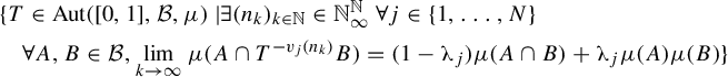
is a dense $G_{\!\delta }$
set.
$G_{\!\delta }$
set.
Theorem 1.2 below, which we prove in §5, extends Theorem 1.1 to any real numbers $\unicode{x3bb} _1,\ldots ,\unicode{x3bb} _N\in [0,1]$
and arbitrary asymptotically linearly independent sequences
$\unicode{x3bb} _1,\ldots ,\unicode{x3bb} _N\in [0,1]$
and arbitrary asymptotically linearly independent sequences $\phi _1,\ldots ,\phi _N:\mathbb {N}\rightarrow \mathbb {Z}$
. The sequences
$\phi _1,\ldots ,\phi _N:\mathbb {N}\rightarrow \mathbb {Z}$
. The sequences $\phi _1,\ldots ,\phi _N$
are asymptotically (linearly) independent if for any
$\phi _1,\ldots ,\phi _N$
are asymptotically (linearly) independent if for any $\vec a=(a_1,\ldots ,a_N)\in \mathbb {Z}^N\setminus \{\vec 0\}$
,
$\vec a=(a_1,\ldots ,a_N)\in \mathbb {Z}^N\setminus \{\vec 0\}$
,
 $$ \begin{align*}\lim_{n\rightarrow\infty}\bigg|\sum_{j=1}^Na_j\phi_j(n)\bigg|=\infty.\end{align*} $$
Theorem 1.2. Let $N\in \mathbb {N}$
and let
$N\in \mathbb {N}$
and let $\unicode{x3bb} _1,\ldots ,\unicode{x3bb} _N\in [0,1]$
. For any asymptotically independent sequences
$\unicode{x3bb} _1,\ldots ,\unicode{x3bb} _N\in [0,1]$
. For any asymptotically independent sequences $\phi _1,\ldots ,\phi _N:\mathbb {N}\rightarrow \mathbb {Z}$
, the set
$\phi _1,\ldots ,\phi _N:\mathbb {N}\rightarrow \mathbb {Z}$
, the set
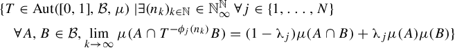
is a dense $G_{\!\delta }$
set.
$G_{\!\delta }$
set.
We will now formulate two results which are needed for the derivation of Theorem 1.2 (see Theorems 1.3 and 1.6 below).
The first of these results is proved by using a modified version of the ‘interpolation’ techniques introduced in [Reference Stëpin11] and can be stated as follows.
Theorem 1.3. Let $N\in \mathbb {N}$
, let
$N\in \mathbb {N}$
, let $\unicode{x3bb} _1,\ldots ,\unicode{x3bb} _N\in [0,1]$
, and let
$\unicode{x3bb} _1,\ldots ,\unicode{x3bb} _N\in [0,1]$
, and let $\phi _1,\ldots ,\phi _N:\mathbb {N}\rightarrow \mathbb {Z}$
. Suppose that
$\phi _1,\ldots ,\phi _N:\mathbb {N}\rightarrow \mathbb {Z}$
. Suppose that $\phi _1,\ldots ,\phi _N$
satisfy the following condition:
$\phi _1,\ldots ,\phi _N$
satisfy the following condition:
Condition C: There exists an $(n_k)_{k\in \mathbb {N}}\in \mathbb {N}^{\mathbb {N}}_\infty $
such that for any
$(n_k)_{k\in \mathbb {N}}\in \mathbb {N}^{\mathbb {N}}_\infty $
such that for any $\vec \xi =(\xi _1,\ldots ,\xi _N)\in \{0,1\}^N$
, there exists an aperiodic
$\vec \xi =(\xi _1,\ldots ,\xi _N)\in \{0,1\}^N$
, there exists an aperiodic $T_{\vec \xi }\in \operatorname {Aut}([0,1],\mathcal B,\mu )$
with the property that for each
$T_{\vec \xi }\in \operatorname {Aut}([0,1],\mathcal B,\mu )$
with the property that for each $j\in \{1,\ldots ,N\}$
and any
$j\in \{1,\ldots ,N\}$
and any $A,B\in \mathcal B$
,
$A,B\in \mathcal B$
,
 $$ \begin{align} \lim_{k\rightarrow\infty}\mu(A\cap T_{\vec \xi}^{- \phi_j(n_k)}B)=(1-\xi_j)\mu(A\cap B)+\xi_j\mu(A)\mu(B). \end{align} $$
Then the set

is a dense $G_{\!\delta }$
set.
$G_{\!\delta }$
set.
To help the reader appreciate the content of Theorem 1.3, let us consider the case $N=1$
. Fix an increasing sequence
$N=1$
. Fix an increasing sequence $(m_k)_{k\in \mathbb {N}}$
in
$(m_k)_{k\in \mathbb {N}}$
in $\mathbb {N}$
and set
$\mathbb {N}$
and set $\phi _1(k)=m_k$
for each
$\phi _1(k)=m_k$
for each $k\in \mathbb {N}$
. We claim that there exists an increasing sequence
$k\in \mathbb {N}$
. We claim that there exists an increasing sequence $(n_k)_{k\in \mathbb {N}}$
in
$(n_k)_{k\in \mathbb {N}}$
in $\mathbb {N}$
for which
$\mathbb {N}$
for which $\phi _1$
satisfies Condition C. In other words, there are transformations
$\phi _1$
satisfies Condition C. In other words, there are transformations $T_0$
and
$T_0$
and $T_1$
such that for any
$T_1$
such that for any $A,B\in \mathcal B$
,
$A,B\in \mathcal B$
,
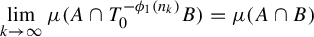 $$ \begin{align} \lim_{k\rightarrow\infty}\mu(A\cap T_0^{-\phi_1(n_k)}B)=\mu(A\cap B) \end{align} $$
and
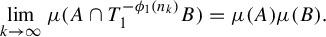 $$ \begin{align} \lim_{k\rightarrow\infty}\mu(A\cap T_1^{-\phi_1(n_k)}B)=\mu(A)\mu(B). \end{align} $$
Note that the set
![]() is a dense
is a dense $G_{\!\delta }$
subset of
$G_{\!\delta }$
subset of $\mathbb {R}$
. Thus, we can pick an irrational
$\mathbb {R}$
. Thus, we can pick an irrational $\alpha $
and an increasing sequence
$\alpha $
and an increasing sequence $(n_k)_{k\in \mathbb {N}}$
such that
$(n_k)_{k\in \mathbb {N}}$
such that $\lim _{k\rightarrow \infty }(\phi _1(n_k)\alpha \,\text {mod}\,1)=0$
. Letting
$\lim _{k\rightarrow \infty }(\phi _1(n_k)\alpha \,\text {mod}\,1)=0$
. Letting $T_0$
be the (aperiodic) transformation defined by
$T_0$
be the (aperiodic) transformation defined by $T_0(x)=(x+\alpha )\,\text {mod}\,1$
, we have that
$T_0(x)=(x+\alpha )\,\text {mod}\,1$
, we have that $T_0$
satisfies (1.5). Our claim now follows by noting that any strongly mixing transformation
$T_0$
satisfies (1.5). Our claim now follows by noting that any strongly mixing transformation $T\in \operatorname {Aut}([0,1],\mathcal B,\mu )$
is aperiodic and satisfies (1.6). (Let
$T\in \operatorname {Aut}([0,1],\mathcal B,\mu )$
is aperiodic and satisfies (1.6). (Let $(X,\mathcal F,\nu )$
be a probability space. A measure-preserving transformation
$(X,\mathcal F,\nu )$
be a probability space. A measure-preserving transformation $T:X\rightarrow X$
is called strongly mixing if for any
$T:X\rightarrow X$
is called strongly mixing if for any $A,B\in \mathcal F$
,
$A,B\in \mathcal F$
, $\lim _{n\rightarrow \infty }\nu (A\cap T^{-n}B)=\nu (A)\nu (B).$
)
$\lim _{n\rightarrow \infty }\nu (A\cap T^{-n}B)=\nu (A)\nu (B).$
)
The above discussion leads to the following corollary to Theorem 1.3. (Corollary 1.4 below is a refinement of the result due to Stëpin mentioned above.)
Corollary 1.4. Let $(m_k)_{k\in \mathbb {N}}$
be an increasing sequence in
$(m_k)_{k\in \mathbb {N}}$
be an increasing sequence in $\mathbb {N}$
and let
$\mathbb {N}$
and let $\unicode{x3bb} \in [0,1]$
. Then
$\unicode{x3bb} \in [0,1]$
. Then
 $$ \begin{align*} &\{T\in\operatorname{Aut}([0,1],\mathcal B,\mu)\,|\exists (k_\ell)_{\ell\in\mathbb{N}}\in\mathbb{N}^{\mathbb{N}}_\infty\,\forall A,B\in\mathcal B,\\ &\qquad\qquad\qquad\qquad\qquad\qquad\lim_{\ell\rightarrow\infty}\mu(A\cap T^{-m_{k_\ell}}B)=(1-\unicode{x3bb})\mu(A\cap B)+\unicode{x3bb}\mu(A)\mu(B)\} \end{align*} $$
is a dense $G_{\!\delta }$
set.
$G_{\!\delta }$
set.
Remark 1.5
-
(1) The special case of Corollary 1.4 corresponding to $\unicode{x3bb} =0$
gives an equivalent form of Proposition 2.8 in [Reference Bergelson, Kasjan and Lemańczyk2], which states that given an increasing sequence
$(m_k)_{k\in \mathbb {N}}$
in
$\mathbb {N}$
, the set is residual.
$$ \begin{align*} \{T\in\operatorname{Aut}([0,1],\mathcal B,\mu)\,|&\exists (k_\ell)_{\ell\in\mathbb{N}}\in\mathbb{N}^{\mathbb{N}}_\infty\,\forall A,B\in\mathcal B,\\&\quad\lim_{\ell\rightarrow\infty}\mu(A\cap T^{-m_{k_\ell}}B)=\mu(A\cap B)\} \end{align*} $$
$\unicode{x3bb} =0$
gives an equivalent form of Proposition 2.8 in [Reference Bergelson, Kasjan and Lemańczyk2], which states that given an increasing sequence
$(m_k)_{k\in \mathbb {N}}$
in
$\mathbb {N}$
, the set is residual.
$$ \begin{align*} \{T\in\operatorname{Aut}([0,1],\mathcal B,\mu)\,|&\exists (k_\ell)_{\ell\in\mathbb{N}}\in\mathbb{N}^{\mathbb{N}}_\infty\,\forall A,B\in\mathcal B,\\&\quad\lim_{\ell\rightarrow\infty}\mu(A\cap T^{-m_{k_\ell}}B)=\mu(A\cap B)\} \end{align*} $$
-
(2) The special case of Corollary 1.4 corresponding to
$\unicode{x3bb} =1$
gives an equivalent form of the ‘folklore theorem’ in [Reference Bergelson, del Junco, Lemańczyk and Rosenblatt1, Proposition 2.14], which states that given an increasing sequence
$(m_k)_{k\in \mathbb {N}}$
in
$\mathbb {N}$
, the set is residual.
$$ \begin{align*} \{T\in\operatorname{Aut}([0,1],\mathcal B,\mu)\,| &\exists (k_\ell)_{\ell\in\mathbb{N}}\in\mathbb{N}^{\mathbb{N}}_\infty\,\forall A,B\in\mathcal B,\\&\quad\lim_{\ell\rightarrow\infty}\mu(A\cap T^{-m_{k_\ell}}B)=\mu(A)\mu(B)\} \end{align*} $$


As we will see below, Condition C in Theorem 1.3 is satisfied by any asymptotically independent sequences $\phi _1,\ldots ,\phi _N:\mathbb {N}\rightarrow \mathbb {Z}$
. We remark in passing that for each
$\phi _1,\ldots ,\phi _N:\mathbb {N}\rightarrow \mathbb {Z}$
. We remark in passing that for each $N\geq 2$
, there exist
$N\geq 2$
, there exist $\mathbb {Q}$
-linearly dependent polynomials
$\mathbb {Q}$
-linearly dependent polynomials $v_1,\ldots ,v_N\in \mathbb {Z}[x]$
for which the (non-asymptotically independent) sequences
$v_1,\ldots ,v_N\in \mathbb {Z}[x]$
for which the (non-asymptotically independent) sequences $(\phi _j(k))_{k\in \mathbb {N}}=(v_j(k))_{k\in \mathbb {N}}$
,
$(\phi _j(k))_{k\in \mathbb {N}}=(v_j(k))_{k\in \mathbb {N}}$
, $j\in \{1,\ldots ,N\}$
, satisfy Condition C. For instance, one can use the results in [Reference Bergelson, Kasjan and Lemańczyk3] to show that
$j\in \{1,\ldots ,N\}$
, satisfy Condition C. For instance, one can use the results in [Reference Bergelson, Kasjan and Lemańczyk3] to show that $\phi _1(n)=2n$
and
$\phi _1(n)=2n$
and $\phi _2(n)=3n$
,
$\phi _2(n)=3n$
, $n\in \mathbb {N}$
, satisfy Condition C. Moreover, one can deduce from [Reference Bergelson, Kasjan and Lemańczyk3] that for any
$n\in \mathbb {N}$
, satisfy Condition C. Moreover, one can deduce from [Reference Bergelson, Kasjan and Lemańczyk3] that for any $N\geq 2$
, the sequences
$N\geq 2$
, the sequences
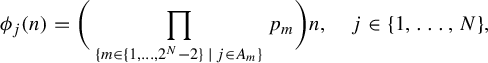 $$ \begin{align*}\phi_j(n)=\bigg(\prod_{\{m\in\{1,\ldots,2^N-2\}\,|\,j\in A_m\}}p_m\bigg)n,\quad j\in\{1,\ldots,N\},\end{align*} $$
where $A_1,\ldots ,A_{2^N-2}$
is an enumeration of the non-empty proper subsets of
$A_1,\ldots ,A_{2^N-2}$
is an enumeration of the non-empty proper subsets of $\{1,\ldots ,N\}$
and
$\{1,\ldots ,N\}$
and $p_1,\ldots ,p_{2^N-2}$
are distinct prime numbers, satisfy Condition C (see also §6 of this paper). For more information on necessary and sufficient conditions for a family of polynomials
$p_1,\ldots ,p_{2^N-2}$
are distinct prime numbers, satisfy Condition C (see also §6 of this paper). For more information on necessary and sufficient conditions for a family of polynomials $\phi _1,\ldots ,\phi _N\in \mathbb {Z}[x]$
to satisfy Condition C, see [Reference Bergelson, Kasjan and Lemańczyk3].
$\phi _1,\ldots ,\phi _N\in \mathbb {Z}[x]$
to satisfy Condition C, see [Reference Bergelson, Kasjan and Lemańczyk3].
The second result needed for the proof of Theorem 1.2 guarantees the existence of measure-preserving transformations for which the sequences $\phi _1,\ldots ,\phi _N:\mathbb {N}\rightarrow \mathbb {Z}$
in Theorem 1.2 satisfy Condition C. Let
$\phi _1,\ldots ,\phi _N:\mathbb {N}\rightarrow \mathbb {Z}$
in Theorem 1.2 satisfy Condition C. Let $(X,\mathcal F,\nu )$
be a probability space. A measure-preserving transformation
$(X,\mathcal F,\nu )$
be a probability space. A measure-preserving transformation $T:X\rightarrow X$
is called weakly mixing if for any
$T:X\rightarrow X$
is called weakly mixing if for any $A,B\in \mathcal F$
,
$A,B\in \mathcal F$
,
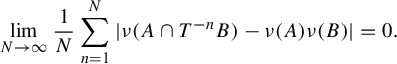 $$ \begin{align*}\lim_{N\rightarrow\infty}\frac{1}{N}\sum_{n=1}^N|\nu(A\cap T^{-n}B)-\nu(A)\nu(B)|=0.\end{align*} $$
Note that every weakly mixing transformation S defined on $([0,1],\mathcal B,\mu )$
is aperiodic.
$([0,1],\mathcal B,\mu )$
is aperiodic.
Theorem 1.6. Let $N\in \mathbb {N}$
and let
$N\in \mathbb {N}$
and let $\phi _1,\ldots ,\phi _N:\mathbb {N}\rightarrow \mathbb {Z}$
be asymptotically independent sequences. Then there exists an increasing sequence
$\phi _1,\ldots ,\phi _N:\mathbb {N}\rightarrow \mathbb {Z}$
be asymptotically independent sequences. Then there exists an increasing sequence $(n_k)_{k\in \mathbb {N}}$
in
$(n_k)_{k\in \mathbb {N}}$
in $\mathbb {N}$
such that for any
$\mathbb {N}$
such that for any $\vec \xi =(\xi _1,\ldots ,\xi _N)\in \{0,1\}^N$
, there exists a weakly mixing
$\vec \xi =(\xi _1,\ldots ,\xi _N)\in \{0,1\}^N$
, there exists a weakly mixing $T_{\vec \xi }\in \operatorname {Aut}([0,1],\mathcal B,\mu )$
with the property that for each
$T_{\vec \xi }\in \operatorname {Aut}([0,1],\mathcal B,\mu )$
with the property that for each $j\in \{1,\ldots ,N\}$
and any
$j\in \{1,\ldots ,N\}$
and any $A,B\in \mathcal B$
,
$A,B\in \mathcal B$
,
 $$ \begin{align} \lim_{k\rightarrow\infty}\mu(A\cap T_{\vec \xi}^{- \phi_j(n_k)}B)=(1-\xi_j)\mu(A\cap B)+\xi_j\mu(A)\mu(B). \end{align} $$
Remark 1.7. When $(\phi _j(k))_{k\in \mathbb {N}}=(v_j(k))_{k\in \mathbb {N}}$
,
$(\phi _j(k))_{k\in \mathbb {N}}=(v_j(k))_{k\in \mathbb {N}}$
, $j\in \{1,\ldots ,N\}$
, for some
$j\in \{1,\ldots ,N\}$
, for some $\mathbb {Q}$
-linearly independent polynomials
$\mathbb {Q}$
-linearly independent polynomials $v_1,\ldots ,v_N\in \mathbb {Z}[x]$
satisfying
$v_1,\ldots ,v_N\in \mathbb {Z}[x]$
satisfying $v_j(0)=0$
, Theorem 1.6 follows from Theorem 3.11 in [Reference Bergelson, Kasjan and Lemańczyk3]. We give an alternative proof of this restricted version of Theorem 1.6 in §3.
$v_j(0)=0$
, Theorem 1.6 follows from Theorem 3.11 in [Reference Bergelson, Kasjan and Lemańczyk3]. We give an alternative proof of this restricted version of Theorem 1.6 in §3.
Consider now the polynomials $v_1,\ldots ,v_N\in \mathbb {Z}[x]$
. We conclude this introduction by formulating a simple corollary of Theorem 1.6 which links the linear independence of the polynomials
$v_1,\ldots ,v_N\in \mathbb {Z}[x]$
. We conclude this introduction by formulating a simple corollary of Theorem 1.6 which links the linear independence of the polynomials $v_1(x)-v_1(0),\ldots ,v_N(x)-v_N(0)\in \mathbb {Z}[x]$
to the possible values of the limits of the form
$v_1(x)-v_1(0),\ldots ,v_N(x)-v_N(0)\in \mathbb {Z}[x]$
to the possible values of the limits of the form
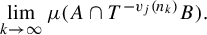 $$ \begin{align*}\lim_{k\rightarrow\infty}\mu(A\cap T^{- v_j(n_k)}B).\end{align*} $$
(Observe that the linear independence of the polynomials $v_1(x)-v_1(0),\ldots ,v_N(x)-v_N(0)$
is equivalent to the asymptotic independence of the sequences
$v_1(x)-v_1(0),\ldots ,v_N(x)-v_N(0)$
is equivalent to the asymptotic independence of the sequences $(v_1(k))_{k\in \mathbb {N}},\ldots , (v_N(k))_{k\in \mathbb {N}}$
.)
$(v_1(k))_{k\in \mathbb {N}},\ldots , (v_N(k))_{k\in \mathbb {N}}$
.)
Corollary 1.8. (Cf. Corollary F in [Reference Bergelson, Kasjan and Lemańczyk3])
Let $N\in \mathbb {N}$
and let
$N\in \mathbb {N}$
and let $t\in \{0,\ldots ,N\}$
. For any non-constant polynomials
$t\in \{0,\ldots ,N\}$
. For any non-constant polynomials $v_1,\ldots ,v_N\in \mathbb {Z}[x]$
such that
$v_1,\ldots ,v_N\in \mathbb {Z}[x]$
such that $v_1(x)-v_1(0),\ldots ,v_N(x)-v_N(0)$
are
$v_1(x)-v_1(0),\ldots ,v_N(x)-v_N(0)$
are $\mathbb {Q}$
-linearly independent, there exists an increasing sequence
$\mathbb {Q}$
-linearly independent, there exists an increasing sequence $(n_k)_{k\in \mathbb {N}}$
in
$(n_k)_{k\in \mathbb {N}}$
in $\mathbb {N}$
and a
$\mathbb {N}$
and a $T\in \operatorname {Aut}([0,1],\mathcal B,\mu )$
with the property that for any
$T\in \operatorname {Aut}([0,1],\mathcal B,\mu )$
with the property that for any $A,B\in \mathcal B$
and any
$A,B\in \mathcal B$
and any $j\in \{1,\ldots ,N\}$
,
$j\in \{1,\ldots ,N\}$
,
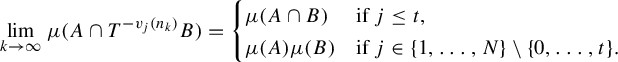 $$ \begin{align*}\lim_{k\rightarrow\infty}\mu(A\cap T^{- v_j(n_k)}B)=\begin{cases} \mu(A\cap B)&\text{if }j\leq t,\\ \mu(A)\mu(B)&\text{if }j\in\{1,\ldots,N\}\setminus\{0,\ldots,t\}. \end{cases}\end{align*} $$
The structure of this paper is as follows. In §2, we introduce the necessary background on Gaussian systems. In §3, we prove a version of Theorem 1.6 dealing with polynomials having zero constant term. In §4, we prove Theorem 1.6. The proof of the special case of Theorem 1.6 given in §3 is quite a bit simpler than, and somewhat different from, the proof of Theorem 1.6 and is of interest on its own. In §5, we prove Theorem 1.3 and obtain Theorem 1.2 as a corollary. In §6, we use a slight modification of the methods introduced in §3 to provide examples of non-asymptotically independent sequences for which Condition C holds.
2 Background on Gaussian systems
In this section, we review the necessary background material on Gaussian systems.
2.1 Basic definitions
Let $\mathcal A=\text {Borel}(\mathbb {R}^{\mathbb {Z}})$
and consider the measurable space
$\mathcal A=\text {Borel}(\mathbb {R}^{\mathbb {Z}})$
and consider the measurable space $(\mathbb {R}^{\mathbb {Z}},\mathcal A)$
. For each
$(\mathbb {R}^{\mathbb {Z}},\mathcal A)$
. For each $n\in \mathbb {Z}$
, we will let
$n\in \mathbb {Z}$
, we will let
 $$ \begin{align} X_n:\mathbb{R}^{\mathbb{Z}}\rightarrow \mathbb{R} \end{align} $$
denote the projection onto the nth coordinate (that is, for each $\omega \in \mathbb {R}^{\mathbb {Z}}$
,
$\omega \in \mathbb {R}^{\mathbb {Z}}$
, $X_n(\omega )=\omega (n)$
).
$X_n(\omega )=\omega (n)$
).
A non-negative Borel measure $\rho $
on
$\rho $
on $\mathbb T=[0,1)$
is called symmetric if for any
$\mathbb T=[0,1)$
is called symmetric if for any $n\in \mathbb {Z}$
,
$n\in \mathbb {Z}$
,
 $$ \begin{align*}\int_{\mathbb T}e^{2\pi inx}\,d\rho(x)=\int_{\mathbb{T}}e^{-2\pi inx}\,d\rho(x).\end{align*} $$
It is well known that for any symmetric non-negative finite Borel measure $\rho $
on
$\rho $
on $\mathbb T$
, there exists a unique probability measure
$\mathbb T$
, there exists a unique probability measure $\gamma =\gamma _{\rho }:\mathcal A\rightarrow [0,1]$
such that: (a) for any
$\gamma =\gamma _{\rho }:\mathcal A\rightarrow [0,1]$
such that: (a) for any $f\in H_1=\overline {\text {span}_{\mathbb {R}}\{X_n\,|\,n\in \mathbb {Z}\}^{L^2(\gamma )}}$
, f has a Gaussian distribution with mean zero (we will treat the constant function
$f\in H_1=\overline {\text {span}_{\mathbb {R}}\{X_n\,|\,n\in \mathbb {Z}\}^{L^2(\gamma )}}$
, f has a Gaussian distribution with mean zero (we will treat the constant function $f\!=0$
as a normal random variable with variance zero); and (b) for any
$f\!=0$
as a normal random variable with variance zero); and (b) for any $m,n\in \mathbb {Z}$
,
$m,n\in \mathbb {Z}$
,
 $$ \begin{align} \int_{\mathbb{R}^{\mathbb{Z}}} X_nX_m\,d\gamma=\int_{\mathbb T}e^{2\pi i(m-n)x}\,d\rho(x). \end{align} $$
We call the probability measure $\gamma $
the Gaussian measure associated with
$\gamma $
the Gaussian measure associated with $\rho $
and refer to
$\rho $
and refer to $\rho $
as the spectral measure associated with
$\rho $
as the spectral measure associated with $\gamma $
. As we will see below, many of the properties of
$\gamma $
. As we will see below, many of the properties of $\rho $
(and hence
$\rho $
(and hence $H_1$
) are intrinsically connected with those of
$H_1$
) are intrinsically connected with those of $\gamma $
.
$\gamma $
.
Let $T:\mathbb {R}^{\mathbb {Z}}\rightarrow \mathbb {R}^{\mathbb {Z}}$
denote the shift map defined by
$T:\mathbb {R}^{\mathbb {Z}}\rightarrow \mathbb {R}^{\mathbb {Z}}$
denote the shift map defined by
 $$ \begin{align*}[T(\omega)](n)=\omega(n+1)\end{align*} $$
for each $\omega \in \mathbb {R}^{\mathbb {Z}}$
and each
$\omega \in \mathbb {R}^{\mathbb {Z}}$
and each $n\in \mathbb {Z}$
. The quadruple
$n\in \mathbb {Z}$
. The quadruple $(\mathbb {R}^{\mathbb {Z}},\mathcal A,\gamma ,T)$
is an invertible probability measure-preserving system called the Gaussian system associated with
$(\mathbb {R}^{\mathbb {Z}},\mathcal A,\gamma ,T)$
is an invertible probability measure-preserving system called the Gaussian system associated with $\rho $
. (For the construction of a Gaussian system, see [Reference Cornfeld, Fomin and Sinai5, Ch. 8] or [Reference Kechris8, Appendix C], for example.)
$\rho $
. (For the construction of a Gaussian system, see [Reference Cornfeld, Fomin and Sinai5, Ch. 8] or [Reference Kechris8, Appendix C], for example.)
Most of the results in the coming sections deal with non-trivial Gaussian systems. A Gaussian system $(\mathbb {R}^{\mathbb {Z}},\mathcal A,\gamma ,T)$
is non-trivial if its spectral measure is not the zero measure. (When
$(\mathbb {R}^{\mathbb {Z}},\mathcal A,\gamma ,T)$
is non-trivial if its spectral measure is not the zero measure. (When $\rho $
is the zero measure, the associated Gaussian system is isomorphic to the probability measure-preserving system with only one point.)
$\rho $
is the zero measure, the associated Gaussian system is isomorphic to the probability measure-preserving system with only one point.)
2.2 Gaussian self-joinings of a Gaussian system
In this subsection, we review the necessary background material on Gaussian self-joinings of Gaussian systems, which were introduced in [Reference Lemańczyk, Parreau and Thouvenot10].
A self-joining of a Gaussian system $(\mathbb {R}^{\mathbb {Z}},\mathcal A,\gamma , T)$
is a (
$(\mathbb {R}^{\mathbb {Z}},\mathcal A,\gamma , T)$
is a ( $T\times T$
)-invariant Borel probability measure
$T\times T$
)-invariant Borel probability measure $\Gamma :\mathcal A\otimes \mathcal A\rightarrow [0,1]$
such that for any
$\Gamma :\mathcal A\otimes \mathcal A\rightarrow [0,1]$
such that for any $A\in \mathcal A$
,
$A\in \mathcal A$
, $\Gamma (\mathbb {R}^{\mathbb {Z}}\times A)=\Gamma (A\times \mathbb {R}^{\mathbb {Z}})=\gamma (A)$
. Denote the set of all self-joinings of
$\Gamma (\mathbb {R}^{\mathbb {Z}}\times A)=\Gamma (A\times \mathbb {R}^{\mathbb {Z}})=\gamma (A)$
. Denote the set of all self-joinings of $(\mathbb {R}^{\mathbb {Z}},\mathcal A,\gamma , T)$
by
$(\mathbb {R}^{\mathbb {Z}},\mathcal A,\gamma , T)$
by $\mathcal J(\gamma )$
. Identifying
$\mathcal J(\gamma )$
. Identifying $\gamma $
with a Borel probability measure on
$\gamma $
with a Borel probability measure on $[0,1]$
, one can view
$[0,1]$
, one can view $\mathcal J(\gamma )$
as a topological subspace of the space of all Borel probability measures on
$\mathcal J(\gamma )$
as a topological subspace of the space of all Borel probability measures on $[0,1]\times [0,1]$
with the weak-* topology. With this topology,
$[0,1]\times [0,1]$
with the weak-* topology. With this topology, $\mathcal J(\gamma )$
is a compact metrizable space with the property that for any sequence
$\mathcal J(\gamma )$
is a compact metrizable space with the property that for any sequence $(\Gamma _k)_{k\in \mathbb {N}}$
in
$(\Gamma _k)_{k\in \mathbb {N}}$
in $\mathcal J(\gamma )$
,
$\mathcal J(\gamma )$
,
 $$ \begin{align*}\lim_{k\rightarrow\infty}\Gamma_k=\Gamma\end{align*} $$
if and only if for every $A,B\in \mathcal A$
,
$A,B\in \mathcal A$
,
 $$ \begin{align} \lim_{k\rightarrow\infty}\Gamma_k(A\times B)=\Gamma(A\times B). \end{align} $$
Remark 2.1. Condition (2.3) is equivalent to the following (seemingly stronger) condition: for any $f,g\in L^2(\gamma )$
,
$f,g\in L^2(\gamma )$
,
 $$ \begin{align*}\lim_{k\rightarrow\infty}\int_{\mathbb{R}^{\mathbb{Z}}\times\mathbb{R}^{\mathbb{Z}}} f(\omega')g(\omega'')\,d\Gamma_k(\omega',\omega'')=\int_{\mathbb{R}^{\mathbb{Z}}\times\mathbb{R}^{\mathbb{Z}}} f(\omega')g(\omega'')\,d\Gamma(\omega',\omega'').\end{align*} $$
Consider now the projections $X^{\prime }_n,X^{\prime \prime }_n:\mathbb {R}^{\mathbb {Z}}\times \mathbb {R}^{\mathbb {Z}}\rightarrow \mathbb {R}$
,
$X^{\prime }_n,X^{\prime \prime }_n:\mathbb {R}^{\mathbb {Z}}\times \mathbb {R}^{\mathbb {Z}}\rightarrow \mathbb {R}$
, $n\in \mathbb {Z}$
, defined by
$n\in \mathbb {Z}$
, defined by
 $$ \begin{align*}X^{\prime}_n(\omega',\omega'')=\omega'(n)\text{ and }X_n''(\omega',\omega'')=\omega''(n)\end{align*} $$
for each $(\omega ',\omega '')\in \mathbb {R}^{\mathbb {Z}}\times \mathbb {R}^{\mathbb {Z}}$
. For any
$(\omega ',\omega '')\in \mathbb {R}^{\mathbb {Z}}\times \mathbb {R}^{\mathbb {Z}}$
. For any $\Gamma \in \mathcal J(\gamma )$
, we will let
$\Gamma \in \mathcal J(\gamma )$
, we will let $H_1'$
and
$H_1'$
and $H_1''$
denote the closed real subspaces of
$H_1''$
denote the closed real subspaces of $L^2(\Gamma )$
spanned by
$L^2(\Gamma )$
spanned by $(X^{\prime }_n)_{n\in \mathbb {Z}}$
and
$(X^{\prime }_n)_{n\in \mathbb {Z}}$
and $(X^{\prime \prime }_n)_{n\in \mathbb {Z}}$
, respectively. Note that both
$(X^{\prime \prime }_n)_{n\in \mathbb {Z}}$
, respectively. Note that both $H_1'$
and
$H_1'$
and $H_1''$
depend only on the topology of
$H_1''$
depend only on the topology of $L^2(\gamma )$
and not on the specific choice of
$L^2(\gamma )$
and not on the specific choice of $\Gamma $
.
$\Gamma $
.
Given $\Gamma \in \mathcal J(\gamma )$
, we say that
$\Gamma \in \mathcal J(\gamma )$
, we say that $\Gamma $
is a Gaussian self-joining (of
$\Gamma $
is a Gaussian self-joining (of $(\mathbb {R}^{\mathbb {Z}},\mathcal A,\gamma ,T)$
) if
$(\mathbb {R}^{\mathbb {Z}},\mathcal A,\gamma ,T)$
) if $\overline {H^{\prime }_1+H^{\prime \prime }_1}$
is a Gaussian subspace in
$\overline {H^{\prime }_1+H^{\prime \prime }_1}$
is a Gaussian subspace in $L^2(\Gamma )$
, meaning that for any
$L^2(\Gamma )$
, meaning that for any $f\in \overline {H^{\prime }_1+H^{\prime \prime }_1}$
, f has a Gaussian distribution. Denote the set of all Gaussian self-joinings of
$f\in \overline {H^{\prime }_1+H^{\prime \prime }_1}$
, f has a Gaussian distribution. Denote the set of all Gaussian self-joinings of $\gamma $
by
$\gamma $
by $\mathcal J_G(\gamma )$
. One can show that for any
$\mathcal J_G(\gamma )$
. One can show that for any $\Gamma \in \mathcal J_G(\gamma )$
,
$\Gamma \in \mathcal J_G(\gamma )$
, $\Gamma $
is completely determined by the values of the correlations
$\Gamma $
is completely determined by the values of the correlations
 $$ \begin{align*}\int_{\mathbb{R}^{\mathbb{Z}}\times\mathbb{R}^{\mathbb{Z}}}X_n'X_m''\,d\Gamma,\quad n,m\in\mathbb{Z}.\end{align*} $$
The following are important examples of Gaussian self-joinings of $(\mathbb {R}^{\mathbb {Z}},\mathcal A,\gamma ,T)$
.
$(\mathbb {R}^{\mathbb {Z}},\mathcal A,\gamma ,T)$
.
-
• The product measure
$\gamma \otimes \gamma $
. This measure is characterized by the correlations (2.4)
$$ \begin{align} \int_{\mathbb{R}^{\mathbb{Z}}\times\mathbb{R}^{\mathbb{Z}}}X_n'X_m''\,d\Gamma=0,\quad n,m\in\mathbb{Z}. \end{align} $$
-
• The measure
$\Delta _a$
,
$a\in \mathbb {Z}$
, defined by
$\Delta _a(A\times B)=\gamma (A\cap T^{-a}B)$
for any
$A,B\in \mathcal A$
. This measure is characterized by the correlations (2.5)
$$ \begin{align} \int_{\mathbb{R}^{\mathbb{Z}}\times\mathbb{R}^{\mathbb{Z}}}X_n'X_m''\,d\Gamma=\int_{\mathbb{R}^{\mathbb{Z}}}X_nX_{m+a}\,d\gamma,\quad n,m\in\mathbb{Z}. \end{align} $$


The next proposition was mentioned as a consequence of Theorem 1 in [Reference Lemańczyk, Parreau and Thouvenot10, p. 267].
Proposition 2.2. $\mathcal J_G(\gamma )$
is a closed (and hence compact) subspace of
$\mathcal J_G(\gamma )$
is a closed (and hence compact) subspace of $\mathcal J(\gamma )$
.
$\mathcal J(\gamma )$
.
Proof. Let $(\Gamma _k)_{k\in \mathbb {N}}$
be a sequence in
$(\Gamma _k)_{k\in \mathbb {N}}$
be a sequence in $\mathcal J_G(\gamma )$
such that
$\mathcal J_G(\gamma )$
such that $\lim _{k\rightarrow \infty }\Gamma _k=\Gamma $
for some
$\lim _{k\rightarrow \infty }\Gamma _k=\Gamma $
for some $\Gamma \in \mathcal J(\gamma )$
. Since the limit of Gaussian distributions is again a Gaussian distribution, it suffices to show that for any
$\Gamma \in \mathcal J(\gamma )$
. Since the limit of Gaussian distributions is again a Gaussian distribution, it suffices to show that for any $f_1\in H_1'$
and
$f_1\in H_1'$
and $f_2\in H_1''$
, the probability measure
$f_2\in H_1''$
, the probability measure $\Gamma \circ (f_1+f_2)^{-1}$
has a Gaussian distribution. To prove this, we will compute the characteristic function
$\Gamma \circ (f_1+f_2)^{-1}$
has a Gaussian distribution. To prove this, we will compute the characteristic function $\phi $
of
$\phi $
of $\Gamma \circ (f_1+f_2)^{-1}$
. For each
$\Gamma \circ (f_1+f_2)^{-1}$
. For each $t\in \mathbb {R}$
,
$t\in \mathbb {R}$
,
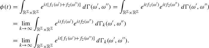 $$ \begin{align} \phi(t)&=\int_{\mathbb{R}^{\mathbb{Z}}\times\mathbb{R}^{\mathbb{Z}}} e^{ it[f_1(\omega')+f_2(\omega'')]}\,d\Gamma(\omega',\omega'')= \int_{\mathbb{R}^{\mathbb{Z}}\times\mathbb{R}^{\mathbb{Z}}} e^{ itf_1(\omega')}e^{itf_2(\omega'')}\,d\Gamma(\omega',\omega'')\nonumber\\ &=\lim_{k\rightarrow\infty}\int_{\mathbb{R}^{\mathbb{Z}}\times\mathbb{R}^{\mathbb{Z}}} e^{ itf_1(\omega')}e^{itf_2(\omega'')}\,d\Gamma_k(\omega',\omega'')\nonumber\\ &= \lim_{k\rightarrow\infty}\int_{\mathbb{R}^{\mathbb{Z}}\times\mathbb{R}^{\mathbb{Z}}} e^{ it[f_1(\omega')+f_2(\omega'')]}\,d\Gamma_k(\omega',\omega''). \end{align} $$
For each $k\in \mathbb {N}$
,
$k\in \mathbb {N}$
, $\Gamma _k\circ (f_1+f_2)^{-1}$
has a Gaussian distribution. Thus, by (2.6),
$\Gamma _k\circ (f_1+f_2)^{-1}$
has a Gaussian distribution. Thus, by (2.6), $\Gamma \circ (f_1+f_2)^{-1}$
has also a Gaussian distribution.
$\Gamma \circ (f_1+f_2)^{-1}$
has also a Gaussian distribution.
2.3 Connections between the mixing properties of
$(\mathbb {R}^{\mathbb {Z}},\mathcal A,\gamma ,T)$
and its spectral measure

Before stating the results in this subsection, we need some definitions.
Let $(X,\mathcal F,\nu , S)$
be an invertible probability measure-preserving system. We say that S has the mixing property along the sequence
$(X,\mathcal F,\nu , S)$
be an invertible probability measure-preserving system. We say that S has the mixing property along the sequence $(n_k)_{k\in \mathbb {N}}$
in
$(n_k)_{k\in \mathbb {N}}$
in $\mathbb {Z}$
if for any
$\mathbb {Z}$
if for any $A,B\in \mathcal F$
,
$A,B\in \mathcal F$
,
 $$ \begin{align*}\lim_{k\rightarrow\infty}\nu(A\cap S^{-n_k}B)=\nu(A)\nu(B).\end{align*} $$
We say that a system $(X,\mathcal F,\nu ,S)$
is rigid along the sequence
$(X,\mathcal F,\nu ,S)$
is rigid along the sequence $(n_k)_{k\in \mathbb {N}}$
in
$(n_k)_{k\in \mathbb {N}}$
in $\mathbb {Z}$
(or equivalently,
$\mathbb {Z}$
(or equivalently, $(n_k)_{k\in \mathbb {N}}$
is a rigidity sequence for
$(n_k)_{k\in \mathbb {N}}$
is a rigidity sequence for $(X,\mathcal F,\nu ,S)$
) if for any
$(X,\mathcal F,\nu ,S)$
) if for any $A,B\in \mathcal F$
,
$A,B\in \mathcal F$
,
 $$ \begin{align*}\lim_{k\rightarrow\infty}\nu(A\cap S^{-n_k}B)=\nu(A\cap B).\end{align*} $$
Now let $\rho $
be a positive finite Borel measure on
$\rho $
be a positive finite Borel measure on $\mathbb T$
and let
$\mathbb T$
and let $(n_k)_{k\in \mathbb {N}}$
be a sequence in
$(n_k)_{k\in \mathbb {N}}$
be a sequence in $\mathbb {Z}$
. We say that
$\mathbb {Z}$
. We say that
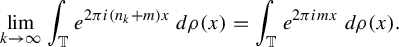
 $\rho $
has the mixing property along the sequence
$\rho $
has the mixing property along the sequence $(n_k)_{k\in \mathbb {N}}$
in
$(n_k)_{k\in \mathbb {N}}$
in $\mathbb {Z}$
if for every
$\mathbb {Z}$
if for every $m\in \mathbb {Z}$
,
$m\in \mathbb {Z}$
,
 $$ \begin{align*}\lim_{k\rightarrow\infty}\int_{\mathbb T} e^{2\pi i (n_k+m)x}\,d\rho(x)=0.\end{align*} $$
We say that $\rho $
is rigid along the sequence
$\rho $
is rigid along the sequence $(n_k)_{k\in \mathbb {N}}$
in
$(n_k)_{k\in \mathbb {N}}$
in $\mathbb {Z}$
if for every
$\mathbb {Z}$
if for every $m\in \mathbb {Z}$
,
$m\in \mathbb {Z}$
,
 $$ \begin{align*}\lim_{k\rightarrow\infty}\int_{\mathbb T} e^{2\pi i (n_k+m)x}\,d\rho(x)=\int_{\mathbb T} e^{2\pi imx}\,d\rho(x).\end{align*} $$
The following result exhibits the close connection between the ‘dynamical’ properties of a spectral measure $\rho $
defined on
$\rho $
defined on $\mathbb T$
and the Gaussian system associated with
$\mathbb T$
and the Gaussian system associated with $\rho $
.
$\rho $
.
Theorem 2.3. Let $\rho $
be a symmetric positive finite Borel measure on
$\rho $
be a symmetric positive finite Borel measure on $\mathbb T$
and let
$\mathbb T$
and let $(\mathbb {R}^{\mathbb {Z}},\mathcal A,\gamma ,T)$
be the Gaussian system associated with it. Given a sequence
$(\mathbb {R}^{\mathbb {Z}},\mathcal A,\gamma ,T)$
be the Gaussian system associated with it. Given a sequence $(n_k)_{k\in \mathbb {N}}$
in
$(n_k)_{k\in \mathbb {N}}$
in $\mathbb {Z}$
, the following statements hold.
$\mathbb {Z}$
, the following statements hold.
-
(i) T has the mixing property along
$(n_k)_{k\in \mathbb {N}}$
if and only if
$\rho $
has the mixing property along
$(n_k)_{k\in \mathbb {N}}$
. -
(ii) T is rigid along
$(n_k)_{k\in \mathbb {N}}$
if and only if
$\rho $
is rigid along
$(n_k)_{k\in \mathbb {N}}$
. -
(iii) Let
$a\in \mathbb {Z}$
. The following are equivalent:-
(1) for every
$A,B\in \mathcal A$
, (2.7)
$$ \begin{align} \lim_{k\rightarrow\infty}\gamma(A\cap T^{-n_k}B)=\gamma(A\cap T^{-a}B); \end{align} $$
-
(2) for every
$m\in \mathbb {Z}$
, (2.8)
$$ \begin{align} \lim_{k\rightarrow\infty}\int_{\mathbb{T}}e^{2\pi i(n_k+m)x}\,d\rho(x)=\int_{\mathbb T} e^{2\pi i(a+m)x}\,d\rho(x). \end{align} $$
-


Proof. The proofs of statements (i), (ii), and (iii) are similar. We will only prove statement (i).
Suppose first that T has the mixing property along $(n_k)_{k\in \mathbb {N}}$
. Then, for any
$(n_k)_{k\in \mathbb {N}}$
. Then, for any $m\in \mathbb {Z}$
,
$m\in \mathbb {Z}$
,
 $$ \begin{align*}\lim_{k\rightarrow\infty}\int_{\mathbb T} e^{2\pi i(n_k+m)x}\,d\rho=\lim_{k\rightarrow\infty}\int_{\mathbb{R}^{\mathbb{Z}}}X_0T^{n_k}X_m\,d\gamma=\int_{\mathbb{R}^{\mathbb{Z}}}X_0\,d\gamma\int_{\mathbb{R}^{\mathbb{Z}}}X_m\,d\gamma=0.\end{align*} $$
Thus, $\rho $
has the mixing property along
$\rho $
has the mixing property along $(n_k)_{k\in \mathbb {N}}$
.
$(n_k)_{k\in \mathbb {N}}$
.
Suppose now that $\rho $
has the mixing property along
$\rho $
has the mixing property along $(n_k)_{k\in \mathbb {N}}$
. Let
$(n_k)_{k\in \mathbb {N}}$
. Let $(k_j)_{j\in \mathbb {N}}$
be an increasing sequence in
$(k_j)_{j\in \mathbb {N}}$
be an increasing sequence in $\mathbb {N}$
such that
$\mathbb {N}$
such that $\lim _{j\rightarrow \infty }\Delta _{n_{k_j}}=\Gamma $
for some
$\lim _{j\rightarrow \infty }\Delta _{n_{k_j}}=\Gamma $
for some $\Gamma \in \mathcal J_G(\gamma )$
. For any
$\Gamma \in \mathcal J_G(\gamma )$
. For any $n,m\in \mathbb {Z}$
, we have
$n,m\in \mathbb {Z}$
, we have
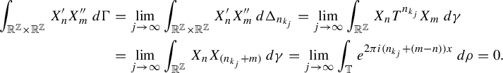 $$ \begin{align*} \int_{\mathbb{R}^{\mathbb{Z}}\times\mathbb{R}^{\mathbb{Z}}}X_n'X_m''\,d\Gamma&=\lim_{j\rightarrow\infty}\int_{\mathbb{R}^{\mathbb{Z}}\times\mathbb{R}^{\mathbb{Z}}}X^{\prime}_nX^{\prime\prime}_m\,d\Delta_{n_{k_j}}=\lim_{j\rightarrow\infty}\int_{\mathbb{R}^{\mathbb{Z}}}X_nT^{n_{k_j}}X_m\,d\gamma\\ &=\lim_{j\rightarrow\infty}\int_{\mathbb{R}^{\mathbb{Z}}}X_nX_{(n_{k_j}+m)}\,d\gamma=\lim_{j\rightarrow\infty}\int_{\mathbb T} e^{2\pi i(n_{k_{j}}+(m-n))x}\,d\rho=0. \end{align*} $$
Thus, by (2.4), $\Gamma =\gamma \otimes \gamma $
. It now follows from the compactness of
$\Gamma =\gamma \otimes \gamma $
. It now follows from the compactness of $\mathcal J_G(\gamma )$
that
$\mathcal J_G(\gamma )$
that $\lim _{k\rightarrow \infty }\Delta _{n_k}=\gamma \otimes \gamma $
. In other words, for any
$\lim _{k\rightarrow \infty }\Delta _{n_k}=\gamma \otimes \gamma $
. In other words, for any $A,B\in \mathcal A$
,
$A,B\in \mathcal A$
,
 $$ \begin{align*}\lim_{k\rightarrow\infty}\gamma(A\cap T^{-n_k}B)=\lim_{k\rightarrow\infty}\Delta_{n_k}(A\times B)=\gamma\otimes \gamma(A\times B)=\gamma(A)\gamma(B).\end{align*} $$
We are done.
We now record for future use the following classical result (see [Reference Cornfeld, Fomin and Sinai5, p. 191] and Theorem 1 in [Reference Cornfeld, Fomin and Sinai5, p. 368], for example).
Proposition 2.4. Let $(\mathbb {R}^{\mathbb {Z}},\mathcal A,\gamma , T)$
be a Gaussian system and let
$(\mathbb {R}^{\mathbb {Z}},\mathcal A,\gamma , T)$
be a Gaussian system and let $\rho $
be the spectral measure associated with it. The following are equivalent: (i)
$\rho $
be the spectral measure associated with it. The following are equivalent: (i) $\rho $
is continuous; (ii) T is weakly mixing; (iii) T is ergodic.
$\rho $
is continuous; (ii) T is weakly mixing; (iii) T is ergodic.
We conclude this section with an easy consequence of Theorem 2.3 which illustrates the connection between non-trivial Gaussian systems and $\operatorname {Aut}([0,1],\mathcal B,\mu )$
.
$\operatorname {Aut}([0,1],\mathcal B,\mu )$
.
Proposition 2.5. Let $(n_k)_{k\in \mathbb {N}}$
be a sequence in
$(n_k)_{k\in \mathbb {N}}$
be a sequence in $\mathbb {Z}$
, let
$\mathbb {Z}$
, let $\xi \in \{0,1\}$
, and let
$\xi \in \{0,1\}$
, and let $a\in \mathbb {Z}$
. The following are equivalent.
$a\in \mathbb {Z}$
. The following are equivalent.
-
(i) There exists a non-trivial Gaussian system
$(\mathbb {R}^{\mathbb {Z}},\mathcal A,\gamma ,T)$
such that for any
$A,B\in \mathcal A$
, (2.9)
$$ \begin{align} \lim_{k\rightarrow\infty}\gamma(A\cap T^{-n_k}B)=(1-\xi)\gamma(A\cap T^{-a} B)+\xi\gamma(A)\gamma(B). \end{align} $$
-
(ii) There exists an
$S\in \operatorname {Aut}([0,1],\mathcal B,\mu )$
such that for any
$A,B\in \mathcal B$
, (2.10)
$$ \begin{align} \lim_{k\rightarrow\infty}\mu(A\cap S^{-n_k}B)=(1-\xi)\mu(A\cap S^{-a} B)+\xi\mu(A)\mu(B). \end{align} $$


Proof. (i) $\implies $
(ii): Note that any non-trivial Gaussian system is measure theoretically isomorphic to
$\implies $
(ii): Note that any non-trivial Gaussian system is measure theoretically isomorphic to $([0,1],\mathcal B,\mu ,S)$
for some
$([0,1],\mathcal B,\mu ,S)$
for some $S\in \operatorname {Aut}([0,1],\beta ,\mu )$
(see [Reference Walters12, Theorem 2.1], for example).
$S\in \operatorname {Aut}([0,1],\beta ,\mu )$
(see [Reference Walters12, Theorem 2.1], for example).
(ii) $\implies $
(i): Let
$\implies $
(i): Let $f\in L^2(\mu )$
be a non-zero real-valued function such that
$f\in L^2(\mu )$
be a non-zero real-valued function such that $\int _{[0,1]}f\,d\mu =0$
and let
$\int _{[0,1]}f\,d\mu =0$
and let $\rho $
be the positive finite Borel measure satisfying
$\rho $
be the positive finite Borel measure satisfying
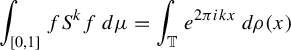 $$ \begin{align*}\int_{[0,1]} fS^kf\,d\mu=\int_{\mathbb T} e^{2\pi i kx}\,d\rho(x)\end{align*} $$
for each $k\in \mathbb {Z}$
. Since
$k\in \mathbb {Z}$
. Since $\int _{\mathbb T} e^{2\pi i kx}\,d\rho (x)$
is a real number for each
$\int _{\mathbb T} e^{2\pi i kx}\,d\rho (x)$
is a real number for each $k\in \mathbb {Z}$
, we have that
$k\in \mathbb {Z}$
, we have that $\rho $
is symmetric.
$\rho $
is symmetric.
By (2.10), for any $g\in L^2(\mu )$
,
$g\in L^2(\mu )$
,
 $$ \begin{align*}\lim_{k\rightarrow\infty}\int_{[0,1]}gS^{n_k}f\,d\mu=(1-\xi)\int_{[0,1]}gS^af\,d\mu+\xi\int_{[0,1]}g\,d\mu\int_{[0,1]}f\,d\mu.\end{align*} $$
Thus, for any $m\in \mathbb {Z}$
,
$m\in \mathbb {Z}$
,
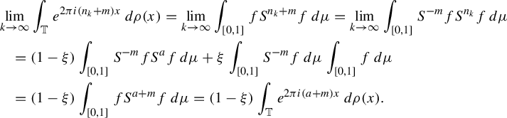 $$ \begin{align*} &\lim_{k\rightarrow\infty}\int_{\mathbb T} e^{2\pi i (n_k+m)x}\,d\rho(x)=\lim_{k\rightarrow\infty}\int_{[0,1]}fS^{n_k+m}f\,d\mu=\lim_{k\rightarrow\infty}\int_{[0,1]}S^{-m}fS^{n_k}f\,d\mu\\ &\quad=(1-\xi)\int_{[0,1]}S^{-m}fS^af\,d\mu+\xi\int_{[0,1]}S^{-m}f\,d\mu\int_{[0,1]}f\,d\mu\\ &\quad=(1-\xi)\int_{[0,1]}fS^{a+m}f\,d\mu =(1-\xi)\int_{\mathbb T} e^{2\pi i(a+m)x}\,d\rho(x). \end{align*} $$
Taking $(\mathbb {R}^{\mathbb {Z}},\mathcal A,\gamma , T)$
to be the non-trivial Gaussian system associated with
$(\mathbb {R}^{\mathbb {Z}},\mathcal A,\gamma , T)$
to be the non-trivial Gaussian system associated with $\rho $
in (i), we see that (2.9) holds.
$\rho $
in (i), we see that (2.9) holds.
3 A version of Theorem 1.6 for polynomials having zero constant term
In this section, we prove a special case of Theorem 1.6 which deals with polynomials $v_1,\ldots ,v_N$
in
$v_1,\ldots ,v_N$
in $\mathbb {Z}[x]$
satisfying
$\mathbb {Z}[x]$
satisfying $v_j(0)=0$
for each
$v_j(0)=0$
for each $j\in \{1,\ldots ,N\}$
. It will be stated in the language of Gaussian systems (see Theorem 3.1 below). Unlike the proof of Theorem 1.6 in its full generality, the proof of this special case uses a simple and explicit construction for the spectral measures associated with each of the Gaussian systems guaranteed to exist in Theorem 3.1. As demonstrated in [Reference Bergelson and Zelada4, Proposition 7.1] and in §6 of this paper, this method can be used to provide examples of measure-preserving systems with various kinds of asymptotic behavior. We remark that while Theorem 1.6 deals with automorphisms of
$j\in \{1,\ldots ,N\}$
. It will be stated in the language of Gaussian systems (see Theorem 3.1 below). Unlike the proof of Theorem 1.6 in its full generality, the proof of this special case uses a simple and explicit construction for the spectral measures associated with each of the Gaussian systems guaranteed to exist in Theorem 3.1. As demonstrated in [Reference Bergelson and Zelada4, Proposition 7.1] and in §6 of this paper, this method can be used to provide examples of measure-preserving systems with various kinds of asymptotic behavior. We remark that while Theorem 1.6 deals with automorphisms of $[0,1]$
, the formulation of Theorem 3.1 deals with non-trivial Gaussian systems
$[0,1]$
, the formulation of Theorem 3.1 deals with non-trivial Gaussian systems $(\mathbb {R}^{\mathbb {Z}},\mathcal A,\gamma ,T)$
. This distinction is immaterial due to a slight modification of Proposition 2.5.
$(\mathbb {R}^{\mathbb {Z}},\mathcal A,\gamma ,T)$
. This distinction is immaterial due to a slight modification of Proposition 2.5.
Theorem 3.1. (Cf. Theorem 1.6)
Let $N\in \mathbb {N}$
, let
$N\in \mathbb {N}$
, let $(m_k)_{k\in \mathbb {N}}$
be an increasing sequence in
$(m_k)_{k\in \mathbb {N}}$
be an increasing sequence in $\mathbb {N}$
with
$\mathbb {N}$
with $k|m_k$
for each
$k|m_k$
for each $k\in \mathbb {N}$
, and let the non-constant polynomials
$k\in \mathbb {N}$
, and let the non-constant polynomials $v_1,\ldots ,v_N\in \mathbb {Z}[x]$
be
$v_1,\ldots ,v_N\in \mathbb {Z}[x]$
be $\mathbb {Q}$
-linearly independent and such that for each
$\mathbb {Q}$
-linearly independent and such that for each $j\in \{1,\ldots ,N\}$
,
$j\in \{1,\ldots ,N\}$
, $v_j(0)=0$
. Then there exists a subsequence
$v_j(0)=0$
. Then there exists a subsequence $(n_k)_{k\in \mathbb {N}}$
of
$(n_k)_{k\in \mathbb {N}}$
of $(m_k)_{k\in \mathbb {N}}$
such that for any
$(m_k)_{k\in \mathbb {N}}$
such that for any $\vec \xi =(\xi _1,\ldots ,\xi _N)\in \{0,1\}^N$
, there exists a non-trivial weakly mixing Gaussian system
$\vec \xi =(\xi _1,\ldots ,\xi _N)\in \{0,1\}^N$
, there exists a non-trivial weakly mixing Gaussian system $(\mathbb {R}^{\mathbb {Z}},\mathcal A,\gamma _{\vec \xi },T_{\vec \xi })$
with the property that for each
$(\mathbb {R}^{\mathbb {Z}},\mathcal A,\gamma _{\vec \xi },T_{\vec \xi })$
with the property that for each $j\in \{1,\ldots ,N\}$
and any
$j\in \{1,\ldots ,N\}$
and any $A,B\in \mathcal A$
,
$A,B\in \mathcal A$
,
 $$ \begin{align} \lim_{k\rightarrow\infty}\gamma_{\kern1.5pt\vec\xi}(A\cap T_{\vec \xi}^{-v_j(n_k)}B)=(1-\xi_j)\gamma_{\kern1.5pt\vec\xi}(A\cap B)+\xi_j\gamma_{\kern1.5pt\vec\xi}(A)\gamma_{\kern1.5pt\vec\xi}(B). \end{align} $$
Proof. By Theorem 2.3 and Proposition 2.4, it suffices to show that there exist a subsequence $(n_k)_{k\in \mathbb {N}}$
of
$(n_k)_{k\in \mathbb {N}}$
of $(m_k)_{k\in \mathbb {N}}$
and continuous Borel probability measures
$(m_k)_{k\in \mathbb {N}}$
and continuous Borel probability measures $\sigma _{\vec \xi }$
on
$\sigma _{\vec \xi }$
on $\mathbb T=[0,1)$
,
$\mathbb T=[0,1)$
, $\vec \xi \in \{0,1\}^N$
, such that for each
$\vec \xi \in \{0,1\}^N$
, such that for each $\vec \xi =(\xi _1,\ldots ,\xi _N)\in \{0,1\}^N$
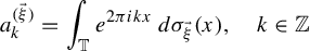
, the sequence
$\vec \xi =(\xi _1,\ldots ,\xi _N)\in \{0,1\}^N$
, the sequence
 $$ \begin{align*}a^{(\vec \xi)}_k=\int_{\mathbb T} e^{2\pi ikx}\,d\sigma_{\vec \xi}(x),\quad k\in\mathbb{Z}\end{align*} $$
is a real-valued sequence with $a^{(\vec \xi )}_0=1$
(which implies that
$a^{(\vec \xi )}_0=1$
(which implies that $\sigma _{\vec \xi }$
is symmetric and non-zero), and for each
$\sigma _{\vec \xi }$
is symmetric and non-zero), and for each $j\in \{1,\ldots ,N\}$
and any
$j\in \{1,\ldots ,N\}$
and any $m\in \mathbb {Z}$
,
$m\in \mathbb {Z}$
,
 $$ \begin{align} \lim_{k\rightarrow\infty}\int_{\mathbb T} e^{2\pi i (v_j(n_k)+m)x}\,d\sigma_{\vec \xi}(x)=(1-\xi_j)\int_{\mathbb T} e^{2\pi i mx}\,d\sigma_{\vec \xi}(x). \end{align} $$
We now proceed to construct the probability measures $\sigma _{\vec \xi }$
,
$\sigma _{\vec \xi }$
, $\vec \xi \in \{0,1\}^N$
, with the desired properties. Let
$\vec \xi \in \{0,1\}^N$
, with the desired properties. Let
 $$ \begin{align*}d=\max _{1\leq j\leq N}\deg v_j\end{align*} $$
and for $j\in \{1,\ldots ,N\}$
, let
$j\in \{1,\ldots ,N\}$
, let $a_{j,1},\ldots ,a_{j,d}\in \mathbb {Z}$
be such that
$a_{j,1},\ldots ,a_{j,d}\in \mathbb {Z}$
be such that
 $$ \begin{align} v_j(x)=\sum_{s=1}^da_{j,s}x^s. \end{align} $$
We define the $N\times d$
matrix D by
$N\times d$
matrix D by
 $$ \begin{align} (D)_{j,s}=a_{j,s} \end{align} $$
for $j\in \{1,\ldots ,N\}$
and
$j\in \{1,\ldots ,N\}$
and $s\in \{1,\ldots ,d\}$
. For each
$s\in \{1,\ldots ,d\}$
. For each $j\in \{1,\ldots ,N\}$
and each
$j\in \{1,\ldots ,N\}$
and each $\vec \xi =(\xi _1,\ldots ,\xi _N)\in \{0,1\}^N$
, let
$\vec \xi =(\xi _1,\ldots ,\xi _N)\in \{0,1\}^N$
, let $b^{(\vec \xi )}_j=1-{\xi _j}/{2}$
and set
$b^{(\vec \xi )}_j=1-{\xi _j}/{2}$
and set
 $$ \begin{align} \vec b_{\vec \xi}=(b^{(\vec \xi)}_1,\ldots,b^{(\vec \xi)}_N). \end{align} $$
Since $v_1,\ldots ,v_N$
are linearly independent, the rank of D is N. Hence, for each
$v_1,\ldots ,v_N$
are linearly independent, the rank of D is N. Hence, for each $\vec \xi \in \{0,1\}^N$
, there exists a non-zero
$\vec \xi \in \{0,1\}^N$
, there exists a non-zero $\vec x_{\vec \xi }=(x^{(\vec \xi )}_1,\ldots ,x^{(\vec \xi )}_d)\in \mathbb {Q}^d$
satisfying
$\vec x_{\vec \xi }=(x^{(\vec \xi )}_1,\ldots ,x^{(\vec \xi )}_d)\in \mathbb {Q}^d$
satisfying
 $$ \begin{align} D\vec x_{\vec \xi}=\vec b_{\vec \xi}. \end{align} $$
Let $n_0\in \mathbb {N}$
be such that
$n_0\in \mathbb {N}$
be such that $n_0>1$
. Choose a subsequence
$n_0>1$
. Choose a subsequence $(n_k)_{k\in \mathbb {N}}$
of
$(n_k)_{k\in \mathbb {N}}$
of $(m_k)_{k\in \mathbb {N}}$
with the property that for any
$(m_k)_{k\in \mathbb {N}}$
with the property that for any $\vec \xi =(\xi _1,\ldots ,\xi _N)\in \{0,1\}^N$
, any
$\vec \xi =(\xi _1,\ldots ,\xi _N)\in \{0,1\}^N$
, any $j\in \{1,\ldots ,d\}$
, and any
$j\in \{1,\ldots ,d\}$
, and any $k\in \mathbb {N}$
: (a)
$k\in \mathbb {N}$
: (a) $dn_0|x_j^{(\vec \xi )}|<n_1$
; (b)
$dn_0|x_j^{(\vec \xi )}|<n_1$
; (b) $x_j^{(\vec \xi )}n_k\in \mathbb {Z}$
; and (c)
$x_j^{(\vec \xi )}n_k\in \mathbb {Z}$
; and (c) $(2dn_{k-1}^{d+1})|n_{k}$
.
$(2dn_{k-1}^{d+1})|n_{k}$
.
Let $\{0,1\}^{\mathbb {N}}$
be endowed with the product topology and let
$\{0,1\}^{\mathbb {N}}$
be endowed with the product topology and let $\mathbb P$
be the
$\mathbb P$
be the $(\tfrac 12,\tfrac 12)$
-probability measure on
$(\tfrac 12,\tfrac 12)$
-probability measure on $\{0,1\}^{\mathbb {N}}$
. For each
$\{0,1\}^{\mathbb {N}}$
. For each $\vec \xi \in \{0,1\}^N$
, we define
$\vec \xi \in \{0,1\}^N$
, we define
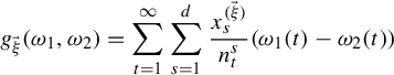
 $f_{\vec \xi }:\{0,1\}^{\mathbb {N}}\times \{0,1\}^{\mathbb {N}}\rightarrow \mathbb T$
by
$f_{\vec \xi }:\{0,1\}^{\mathbb {N}}\times \{0,1\}^{\mathbb {N}}\rightarrow \mathbb T$
by
 $$ \begin{align} f_{\vec \xi}(\omega_1,\omega_2)=\sum_{t=1}^\infty\sum_{s=1}^d\frac{x^{(\vec \xi)}_s}{n_t^s}(\omega_1(t)-\omega_2(t))\, \mod\!1. \end{align} $$
Since for any $\omega _1,\omega _2\in \{0,1\}^{\mathbb {N}}$
and any
$\omega _1,\omega _2\in \{0,1\}^{\mathbb {N}}$
and any $k\in \mathbb {N}$
,
$k\in \mathbb {N}$
, $|\omega _1(k)-\omega _2(k)|\leq 1$
, item (a) implies that for any
$|\omega _1(k)-\omega _2(k)|\leq 1$
, item (a) implies that for any $t\in \mathbb {N}$
and any
$t\in \mathbb {N}$
and any $s\in \{1,\ldots ,d\}$
,
$s\in \{1,\ldots ,d\}$
,
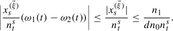 $$ \begin{align*}\bigg|\frac{x^{(\vec \xi)}_s}{n_t^s}(\omega_1(t)-\omega_2(t))\bigg|\leq \frac{|x^{(\vec \xi)}_s|}{n_t^s}\leq \frac{n_1}{dn_0n_t^s}.\end{align*} $$
By item (c),
 $$ \begin{align} \sum_{t=1}^\infty\sum_{s=1}^d\frac{n_1}{dn_0n_t^s}\leq \sum_{t=1}^\infty\frac{dn_1}{dn_0n_t} =\frac{1}{n_0}\sum_{t=1}^\infty\frac{n_1}{n_t}\leq \frac{1}{n_0}\sum_{t=0}^\infty\frac{1}{n_1^t}=\frac{1}{n_0}\frac{n_1}{n_1-1}\leq 1. \end{align} $$
Thus, by Weierstrass M-test, the function $g_{\vec \xi }:\{0,1\}^{\mathbb {N}}\times \{0,1\}^{\mathbb {N}}\rightarrow \mathbb {R}$
given by
$g_{\vec \xi }:\{0,1\}^{\mathbb {N}}\times \{0,1\}^{\mathbb {N}}\rightarrow \mathbb {R}$
given by
 $$ \begin{align*}g_{\vec \xi}(\omega_1,\omega_2)= \sum_{t=1}^\infty\sum_{s=1}^d\frac{x^{(\vec \xi)}_s}{n_t^s}(\omega_1(t)-\omega_2(t))\end{align*} $$
is well defined and continuous.
Let $\phi $
be the canonical map from
$\phi $
be the canonical map from $\mathbb {R}$
to
$\mathbb {R}$
to $[0,1)=\mathbb {R}/\mathbb {Z}$
(so
$[0,1)=\mathbb {R}/\mathbb {Z}$
(so $\phi (x)=x\,\mod \!1$
and
$\phi (x)=x\,\mod \!1$
and $\phi $
is continuous). Since
$\phi $
is continuous). Since $f_{\vec \xi }=\phi \circ g_{\vec \xi }$
, we have that
$f_{\vec \xi }=\phi \circ g_{\vec \xi }$
, we have that $f_{\vec \xi }$
is continuous and hence measurable. For each
$f_{\vec \xi }$
is continuous and hence measurable. For each $\vec \xi \in \{0,1\}^N$
, we will let
$\vec \xi \in \{0,1\}^N$
, we will let
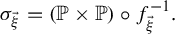 $$ \begin{align*}\sigma_{\vec \xi}=(\mathbb P\times \mathbb P)\circ f_{\vec \xi}^{-1}.\end{align*} $$
Fix now $\vec \xi =(\xi _1,\ldots ,\xi _N)\in \{0,1\}^N$
. Clearly
$\vec \xi =(\xi _1,\ldots ,\xi _N)\in \{0,1\}^N$
. Clearly $\sigma _{\vec \xi }$
is a Borel probability measure on
$\sigma _{\vec \xi }$
is a Borel probability measure on $\mathbb T$
(and so,
$\mathbb T$
(and so, $a^{(\vec \xi )}_0=1$
). All it remains to show is that: (i)
$a^{(\vec \xi )}_0=1$
). All it remains to show is that: (i) $\sigma _{\vec \xi }$
is continuous; (ii)
$\sigma _{\vec \xi }$
is continuous; (ii) $(a^{(\vec \xi )}_k)_{k\in \mathbb {Z}}$
is real-valued; and (iii)
$(a^{(\vec \xi )}_k)_{k\in \mathbb {Z}}$
is real-valued; and (iii) $\sigma _{\vec \xi }$
satisfies (3.2). For this, let
$\sigma _{\vec \xi }$
satisfies (3.2). For this, let $f:\{0,1\}^{\mathbb {N}}\rightarrow \mathbb {R}$
be defined by
$f:\{0,1\}^{\mathbb {N}}\rightarrow \mathbb {R}$
be defined by
 $$ \begin{align*}f(\omega)=\sum_{t=1}^\infty\sum_{s=1}^d\frac{x^{(\vec \xi)}_s}{n_t^s}\frac{\omega(t)}{2}.\end{align*} $$
(Note that by an inequality similar to (3.8), one can show that f is well defined and continuous).
(i) We will now show that $\sigma _{\vec \xi }$
is continuous, but first we need some estimates.
$\sigma _{\vec \xi }$
is continuous, but first we need some estimates.
Combining items (b) and (c), we obtain that for each $\ell \in \{1,\ldots ,d\}$
, each
$\ell \in \{1,\ldots ,d\}$
, each $\omega \in \{0,1\}^{\mathbb {N}}$
, and each
$\omega \in \{0,1\}^{\mathbb {N}}$
, and each $k>1$
,
$k>1$
,
 $$ \begin{align} &n_k^{\ell}f(\omega)\,\text{mod}\,1 \equiv n_k^\ell\bigg(\sum_{t=1}^\infty\sum_{s=1}^d\frac{x^{(\vec \xi)}_s}{n_t^s}\frac{\omega(t)}{2}\bigg)\equiv \sum_{t=1}^\infty\sum_{s=1}^d\frac{n_k^\ell x^{(\vec \xi)}_s}{n_t^s}\frac{\omega(t)}{2}\nonumber\\&\quad\equiv \underbrace{\sum_{t=1}^{k-1}\sum_{s=1}^d\frac{n_k^\ell x^{(\vec \xi)}_s}{n_t^{s}}\frac{\omega(t)}{2}}_{\text{This is an integer}}+\!\underbrace{\sum_{s=1}^{\ell-1}\frac{n_k^\ell x^{(\vec \xi)}_s}{n_k^{s}}\frac{\omega(k)}{2}}_{\text{This is an integer}}+\!\sum_{s=\ell}^d\frac{x^{(\vec \xi)}_s}{n_k^{s-\ell}}\frac{\omega(k)}{2}+\!\sum_{t=k+1}^\infty\sum_{s=1}^d\frac{n_k^\ell x^{(\vec \xi)}_s}{n_t^{s}}\frac{\omega(t)}{2}\nonumber\\&\quad\equiv x^{(\vec \xi)}_\ell\frac{\omega(k)}{2}+\sum_{s=\ell+1}^d\frac{x^{(\vec \xi)}_s}{n_k^{s-\ell}}\frac{\omega(k)}{2}+\sum_{t=k+1}^\infty\sum_{s=1}^d\frac{n_k^\ell x^{(\vec \xi)}_s}{n_t^{s}}\frac{\omega(t)}{2} \,\mod\!1. \end{align} $$
By items (a) and (c), we have
 $$ \begin{align} &\bigg|\sum_{s=\ell+1}^d\frac{x^{(\vec \xi)}_s}{n_k^{s-\ell}}\frac{\omega(k)}{2}+\sum_{t=k+1}^\infty\sum_{s=1}^d\frac{n_k^\ell x^{(\vec \xi)}_s}{n_t^{s}}\frac{\omega(t)}{2}\bigg|\leq \sum_{s=\ell+1}^d\frac{n_1}{n_k^{s-\ell}}+\sum_{t=k+1}^\infty\frac{n_k^\ell n_1}{n_t}\nonumber\\ &\quad\leq \sum_{t=1}^d\frac{n_1}{n_k^t}+\sum_{t=1}^\infty\frac{n_1}{n_k^t}\leq 2n_1\sum_{t=1}^\infty\frac{1}{n_k^t}=\frac{2n_1}{n_k-1}. \end{align} $$
(Note that when $\ell =d$
,
$\ell =d$
, $|\sum _{t=k+1}^\infty \sum _{s=1}^d({n_k^\ell x^{(\vec \xi )}_s}/{n_t^{s}}){\omega (t)}/{2}|<{2n_1}/{(n_k-1)}$
also holds.)
$|\sum _{t=k+1}^\infty \sum _{s=1}^d({n_k^\ell x^{(\vec \xi )}_s}/{n_t^{s}}){\omega (t)}/{2}|<{2n_1}/{(n_k-1)}$
also holds.)
Denote the distance to the closest integer by $\|\cdot \|$
(so for any
$\|\cdot \|$
(so for any $r\in \mathbb {R}$
,
$r\in \mathbb {R}$
, $\|r\|= \inf _{n\in \mathbb {Z}} |r-n|$
and, in particular,
$\|r\|= \inf _{n\in \mathbb {Z}} |r-n|$
and, in particular, $\|r\|\leq |r|$
). Consider a polynomial with integer coefficients
$\|r\|\leq |r|$
). Consider a polynomial with integer coefficients $v(n)=\sum _{\ell =1}^da_\ell n^\ell $
. By (3.9) and (3.10), for any
$v(n)=\sum _{\ell =1}^da_\ell n^\ell $
. By (3.9) and (3.10), for any $k>1$
and any
$k>1$
and any $\omega \in \{0,1\}^{\mathbb {N}}$
,
$\omega \in \{0,1\}^{\mathbb {N}}$
,
 $$ \begin{align*} &\bigg\|v(n_k)f(\omega)-\sum_{\ell=1}^da_{\ell}x^{(\vec \xi)}_\ell\frac{\omega(k)}{2}\bigg\| =\bigg\|\sum_{\ell=1}^d a_\ell\bigg[n_k^{\ell}f(\omega)-x^{(\vec \xi)}_\ell\frac{\omega(k)}{2}\bigg]\bigg\|\\[5pt]&\quad\leq \sum_{\ell=1}^d|a_\ell|\bigg\|n_k^\ell f(\omega)-x^{(\vec \xi)}_\ell\frac{\omega(k)}{2}\bigg\|\\[5pt]&\quad=\sum_{\ell=1}^d|a_{\ell}|\bigg\|\sum_{s=\ell+1}^d\frac{x^{(\vec \xi)}_s}{n_k^{s-\ell}}\frac{\omega(k)}{2}+\sum_{t=k+1}^\infty\sum_{s=1}^d\frac{n_k^\ell x^{(\vec \xi)}_s}{n_t^{s}}\frac{\omega(t)}{2}\bigg\|\\[5pt]&\quad\leq \sum_{\ell=1}^d|a_{\ell}|\bigg|\sum_{s=\ell+1}^d\frac{x^{(\vec \xi)}_s}{n_k^{s-\ell}}\frac{\omega(k)}{2}+\sum_{t=k+1}^\infty\sum_{s=1}^d\frac{n_k^\ell x^{(\vec \xi)}_s}{n_t^{s}}\frac{\omega(t)}{2}\bigg| \leq \sum_{\ell=1}^d|a_{\ell}|\bigg(\frac{2n_1}{n_k-1}\bigg). \end{align*} $$
Thus, for any $\epsilon>0$
, there exists
$\epsilon>0$
, there exists $k_\epsilon \in \mathbb {N}$
such that for any
$k_\epsilon \in \mathbb {N}$
such that for any $k>k_\epsilon $
and any
$k>k_\epsilon $
and any $\omega \in \{0,1\}^{\mathbb {N}}$
,
$\omega \in \{0,1\}^{\mathbb {N}}$
,
 $$ \begin{align} \bigg\|v(n_k)f(\omega)-\sum_{\ell=1}^da_{\ell}x^{(\vec \xi)}_\ell\frac{\omega(k)}{2}\bigg\|<\epsilon. \end{align} $$
Pick now $\alpha \in \mathbb {R}$
and suppose that there exists an
$\alpha \in \mathbb {R}$
and suppose that there exists an $\omega _\alpha \in \{0,1\}^{\mathbb {N}}$
such that
$\omega _\alpha \in \{0,1\}^{\mathbb {N}}$
such that $f(\omega _\alpha )\equiv \alpha \, \mod \!1$
. By (3.11), there exists
$f(\omega _\alpha )\equiv \alpha \, \mod \!1$
. By (3.11), there exists $k_{1/8}\in \mathbb {N}$
such that for any
$k_{1/8}\in \mathbb {N}$
such that for any $k>k_{1/8}$
and any
$k>k_{1/8}$
and any $\omega \in \{0,1\}^{\mathbb {N}}$
with
$\omega \in \{0,1\}^{\mathbb {N}}$
with $f(\omega )\equiv \alpha \, \mod \!1$
,
$f(\omega )\equiv \alpha \, \mod \!1$
,
 $$ \begin{align*} &\bigg\|\bigg(1-\frac{\xi_1}{2}\bigg)\frac{\omega(k)-\omega_\alpha(k)}{2}\bigg\|=\bigg\|b_1^{(\vec \xi)}\frac{\omega(k)-\omega_\alpha(k)}{2}\bigg\|=\bigg\|\sum_{\ell=1}^da_{1,\ell}x^{(\vec \xi)}_\ell\frac{\omega(k)-\omega_\alpha(k)}{2}\bigg\|\\[5pt]&\quad\leq \bigg\|\sum_{\ell=1}^da_{1,\ell}x^{(\vec \xi)}_\ell\frac{\omega(k)-\omega_\alpha(k)}{2}-v_1(n_k)(f(\omega)-\kern-1.5pt f(\omega_\alpha))\bigg\|\kern-2pt +\|v_1(n_k)(f(\omega)-\kern-1.5pt f(\omega_\alpha))\| \\[5pt]&\quad\leq \bigg\|\sum_{\ell=1}^da_{1,\ell}x^{(\vec \xi)}_\ell\frac{\omega(k)}{2}-v_1(n_k)f(\omega)\bigg\|+\bigg\|\sum_{\ell=1}^da_{1,\ell}x^{(\vec \xi)}_\ell\frac{\omega_\alpha(k)}{2}-v_1(n_k)f(\omega_\alpha)\bigg\|\\[5pt]&\qquad+\|v_1(n_k)(f(\omega)-f(\omega_\alpha))\|\\&\quad<\frac{1}{8}+\frac{1}{8}+ \|v_1(n_k)(f(\omega)-f(\omega_\alpha))\|=\frac{1}{4}+0=\frac{1}{4}. \end{align*} $$
Note that if $\omega (k)\neq \omega _\alpha (k)$
, then
$\omega (k)\neq \omega _\alpha (k)$
, then $|(1-{\xi _1}/{2})({\omega (k)-\omega _\alpha (k)})/{2}|\in \{\tfrac 14,\tfrac 12\}$
. Since for any
$|(1-{\xi _1}/{2})({\omega (k)-\omega _\alpha (k)})/{2}|\in \{\tfrac 14,\tfrac 12\}$
. Since for any $k>k_{1/8}$
,
$k>k_{1/8}$
,
 $$ \begin{align*}\bigg|\bigg(1-\frac{\xi_1}{2}\bigg)\frac{\omega(k)-\omega_\alpha(k)}{2}\bigg|=\bigg\|\bigg(1-\frac{\xi_1}{2}\bigg)\frac{\omega(k)-\omega_\alpha(k)}{2}\bigg\|<\frac{1}{4},\end{align*} $$
we have $|(1-{\xi _1}/{2})({\omega (k)-\omega _\alpha (k)})/{2}|\not \in \{\tfrac 14,\tfrac 12\}$
and hence
$|(1-{\xi _1}/{2})({\omega (k)-\omega _\alpha (k)})/{2}|\not \in \{\tfrac 14,\tfrac 12\}$
and hence $\omega (k)=\omega _\alpha (k)$
. It follows that
$\omega (k)=\omega _\alpha (k)$
. It follows that $f^{-1}(\{\alpha +n\,|\,n\in \mathbb {Z}\})$
is a subset of
$f^{-1}(\{\alpha +n\,|\,n\in \mathbb {Z}\})$
is a subset of
 $$ \begin{align*}\{\omega\in\{0,1\}^{\mathbb{N}}\,|\forall k>k_{1/8},\,\omega(k)=\omega_\alpha(k)\},\end{align*} $$
which has at most $2^{k_{1/8}}$
elements.
$2^{k_{1/8}}$
elements.
Let $g:\{0,1\}^{\mathbb {N}}\rightarrow \mathbb T$
be defined by
$g:\{0,1\}^{\mathbb {N}}\rightarrow \mathbb T$
be defined by
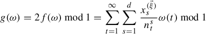 $$ \begin{align*}g(\omega)=2f(\omega)\,\text{mod}\,1=\sum_{t=1}^\infty\sum_{s=1}^d\frac{x^{(\vec \xi)}_s}{n_t^s}\omega(t)\, \mod\!1\end{align*} $$
and set
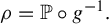 $$ \begin{align*}\rho=\mathbb P\circ g^{-1}.\end{align*} $$
Take $\alpha \in [0,1)$
and let
$\alpha \in [0,1)$
and let $x={\alpha }/{2}$
. Regarding
$x={\alpha }/{2}$
. Regarding $\alpha $
as an element of
$\alpha $
as an element of $\mathbb T=\mathbb {R}/\mathbb {Z}$
, we have
$\mathbb T=\mathbb {R}/\mathbb {Z}$
, we have
 $$ \begin{align*}g^{-1}(\{\alpha\})=f^{-1}(\{x+n\,|\,n\in\mathbb{Z}\})\cup f^{-1}\big(\big\{x+\tfrac{1}{2}+n\,\big|\,n\in\mathbb{Z}\big\}\big).\end{align*} $$
It follows that $g^{-1}(\{\alpha \})$
is finite and hence
$g^{-1}(\{\alpha \})$
is finite and hence
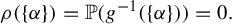 $$ \begin{align*}\rho(\{\alpha\})=\mathbb P(g^{-1}(\{\alpha\}))=0.\end{align*} $$
Noting that $f_{\vec \xi }(\omega _1,\omega _2)=g(\omega _1)-g(\omega _2)$
, we have
$f_{\vec \xi }(\omega _1,\omega _2)=g(\omega _1)-g(\omega _2)$
, we have
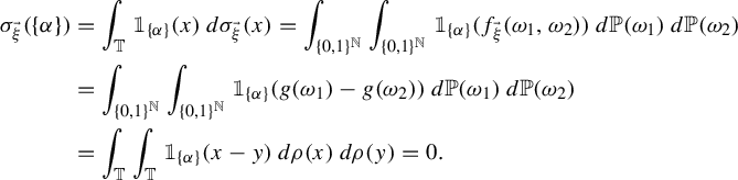
So, $\sigma _{\vec \xi }$
is continuous.
$\sigma _{\vec \xi }$
is continuous.
(ii) For each $m\in \mathbb {Z}$
,
$m\in \mathbb {Z}$
,
 $$ \begin{align} \int_{\mathbb T} e^{2\pi imx}\,d\sigma_{\vec \xi}(x)=\int_{\mathbb T} \int_{\mathbb T} e^{2\pi i m(x-y)}\,d\rho(x)\,d\rho(y)=\bigg|\int_{\mathbb T} e^{2\pi im x}\,d\rho(x)\bigg|^2. \end{align} $$
Thus, the sequence $(a_k^{(\vec \xi )})_{k\in \mathbb {Z}}$
is real valued.
$(a_k^{(\vec \xi )})_{k\in \mathbb {Z}}$
is real valued.
(iii) Finally, we show that $\sigma _{\vec \xi }$
satisfies (3.2). By (3.11) and the definitions of g, D,
$\sigma _{\vec \xi }$
satisfies (3.2). By (3.11) and the definitions of g, D, $\vec x_{\vec \xi }$
, and
$\vec x_{\vec \xi }$
, and $\vec b_{\vec \xi }$
, each
$\vec b_{\vec \xi }$
, each $j\in \{1,\ldots ,N\}$
and each
$j\in \{1,\ldots ,N\}$
and each $m\in \mathbb {Z}$
satisfies
$m\in \mathbb {Z}$
satisfies
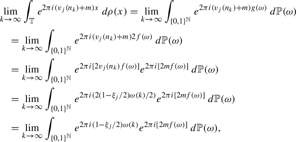 $$ \begin{align} &\lim_{k\rightarrow\infty}\int_{\mathbb T} e^{2\pi i (v_j(n_k)+m)x}\,d\rho(x)=\lim_{k\rightarrow\infty}\int_{\{0,1\}^{\mathbb{N}}} e^{2\pi i (v_j(n_k)+m)g(\omega)}\,d\mathbb P(\omega)\nonumber\\&\quad=\lim_{k\rightarrow\infty}\int_{\{0,1\}^{\mathbb{N}}} e^{2\pi i (v_j(n_k)+m)2f(\omega)}\,d\mathbb P(\omega)\nonumber\\&\quad=\lim_{k\rightarrow\infty}\int_{\{0,1\}^{\mathbb{N}}} e^{2\pi i [2v_j(n_k)f(\omega)]}e^{2\pi i[2m f(\omega)]}\,d\mathbb P(\omega)\nonumber\\&\quad=\lim_{k\rightarrow\infty}\int_{\{0,1\}^{\mathbb{N}}} e^{2\pi i (2(1-{\xi_j}/{2}){\omega(k)}/{2})}e^{2\pi i[2mf(\omega)]}\,d\mathbb P(\omega)\nonumber\\&\quad=\lim_{k\rightarrow\infty}\int_{\{0,1\}^{\mathbb{N}}} e^{2\pi i(1-{\xi_j}/{2})\omega(k)}e^{2\pi i[2mf(\omega)]}\,d\mathbb P(\omega), \end{align} $$
whenever any (and hence each) of the limits in (3.13) exist.
Since the shift map on $\{0,1\}^{\mathbb {N}}$
is
$\{0,1\}^{\mathbb {N}}$
is $\mathbb P$
-mixing, the last expression in (3.13) can be rewritten as
$\mathbb P$
-mixing, the last expression in (3.13) can be rewritten as
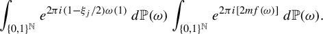 $$ \begin{align} \int_{\{0,1\}^{\mathbb{N}}} e^{2\pi i(1-{\xi_j}/{2})\omega(1)}\,d\mathbb P(\omega)\int_{\{0,1\}^{\mathbb{N}}} e^{2\pi i[2mf(\omega)]}\,d\mathbb P(\omega). \end{align} $$
Since $\omega (1)$
equals each of
$\omega (1)$
equals each of $1$
and
$1$
and $0$
with probability
$0$
with probability $\tfrac 12$
, we get that (3.14) equals
$\tfrac 12$
, we get that (3.14) equals
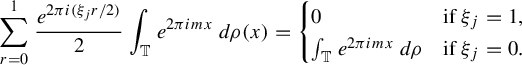 $$ \begin{align*}\sum_{r=0}^1\frac{e^{2\pi i({\xi_jr}/{2})}}{2}\int_{\mathbb T} e^{2\pi imx}\,d\rho(x)=\begin{cases} 0&\text{if }\xi_j=1,\\ \int_{\mathbb T} e^{2\pi imx}\,d\rho&\text{if }\xi_j=0. \end{cases}\end{align*} $$
So, by (3.12),
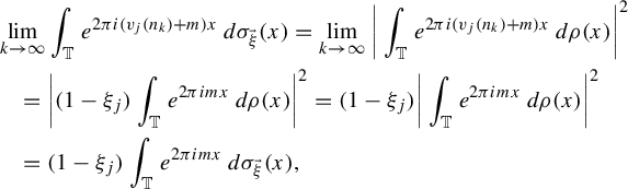 $$ \begin{align*} &\lim_{k\rightarrow\infty}\int_{\mathbb T} e^{2\pi i (v_j(n_k)+m)x}\,d\sigma_{\vec \xi}(x)=\lim_{k\rightarrow\infty}\bigg|\int_{\mathbb T} e^{2\pi i (v_j(n_k)+m)x}\,d\rho(x)\bigg|^2\\ &\quad=\bigg|(1-\xi_j)\int_{\mathbb T} e^{2\pi imx}\,d\rho(x)\bigg|^2=(1-\xi_j)\bigg|\int_{\mathbb T} e^{2\pi imx}\,d\rho(x)\bigg|^2\\ &\quad=(1-\xi_j)\int_{\mathbb T} e^{2\pi imx}\,d\sigma_{\vec \xi}(x), \end{align*} $$
proving that (3.2) holds.
4 The proof of Theorem 1.6
In this section, we prove Theorem 1.6 (=Theorem 4.2 below) on its full generality. First, we need a technical lemma.
Given any sequences $\phi _1,\ldots ,\phi _N:\mathbb {N}\rightarrow \mathbb {Z}$
, we say that the sequences
$\phi _1,\ldots ,\phi _N:\mathbb {N}\rightarrow \mathbb {Z}$
, we say that the sequences $\phi _1,\ldots ,\phi _N$
are strongly asymptotically independent if for any
$\phi _1,\ldots ,\phi _N$
are strongly asymptotically independent if for any $\vec a=(a_1,\ldots ,a_N)\in \mathbb {Z}^N\setminus \{\vec 0\}$
, the sequence
$\vec a=(a_1,\ldots ,a_N)\in \mathbb {Z}^N\setminus \{\vec 0\}$
, the sequence
 $$ \begin{align*}a_1\phi_1(k)+\cdots+a_N\phi_N(k),\quad k\in\mathbb{N}\end{align*} $$
is eventually a strictly monotone sequence (so, in particular, $\lim _{k\rightarrow \infty }\kern-2pt |\!\sum _{s=1}^N\kern-1.2pt a_s\phi _s(k)|\!=\infty $
).
$\lim _{k\rightarrow \infty }\kern-2pt |\!\sum _{s=1}^N\kern-1.2pt a_s\phi _s(k)|\!=\infty $
).
Lemma 4.1. (Cf. Theorem 21 in [Reference Weyl13])
Let $\phi _1,\ldots ,\phi _N:\mathbb {N}\rightarrow \mathbb {Z}$
be strongly asymptotically independent sequences. For any
$\phi _1,\ldots ,\phi _N:\mathbb {N}\rightarrow \mathbb {Z}$
be strongly asymptotically independent sequences. For any $t\in \mathbb {N}$
, the set
$t\in \mathbb {N}$
, the set
 $$ \begin{align*} \mathfrak M_t(\phi_1,\ldots,\phi_N)&= \{(\alpha_1,\ldots,\alpha_t)\in \mathbb{R}^t\,|\,(\phi_1(k)\alpha_1,\ldots,\phi_N(k)\alpha_1,\ldots,\phi_1(k)\alpha_t,\\&\,\quad\ldots,\phi_N(k)\alpha_t)_{k\in\mathbb{N}}\text{ is uniformly distributed mod}\,1\} \end{align*} $$
has full Lebesgue measure on $\mathbb {R}^t$
. Furthermore, for any
$\mathbb {R}^t$
. Furthermore, for any $(\alpha _1,\ldots ,\alpha _t)\in \mathfrak M_t(\phi _1,\ldots ,\phi _N)$
, the set
$(\alpha _1,\ldots ,\alpha _t)\in \mathfrak M_t(\phi _1,\ldots ,\phi _N)$
, the set
 $$ \begin{align} \mathfrak M(\phi_1,\ldots,\phi_N,\alpha_1,\ldots,\alpha_t)=\{\alpha\in\mathbb{R}\,|\,(\alpha_1,\ldots,\alpha_t,\alpha)\in \mathfrak M_{t+1}(\phi_1,\ldots,\phi_N)\} \end{align} $$
has full measure on $\mathbb {R}$
.
$\mathbb {R}$
.
Proof. To prove the first claim, we will use induction on $t\in \mathbb {N}$
. When
$t\in \mathbb {N}$
. When $t=1$
, the proof is the same as that of Theorem 4.1 in [Reference Kuipers and Niederreiter9]. By Weyl’s criterion for uniform distribution
$t=1$
, the proof is the same as that of Theorem 4.1 in [Reference Kuipers and Niederreiter9]. By Weyl’s criterion for uniform distribution $\mod \!1$
, it suffices to show that for any
$\mod \!1$
, it suffices to show that for any $(a_1,\ldots ,a_N)\in \mathbb {Z}^N\setminus \{\vec 0\}$
, the set
$(a_1,\ldots ,a_N)\in \mathbb {Z}^N\setminus \{\vec 0\}$
, the set
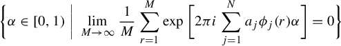 $$ \begin{align*}\bigg\{\alpha\in [0,1)\,\bigg|\,\lim_{M\rightarrow\infty}\frac{1}{M}\sum_{r=1}^M \exp\bigg[2\pi i\sum_{j=1}^N a_j\phi_j(r)\alpha\bigg]=0\bigg\}\end{align*} $$
has Lebesgue measure 1.
For each $M\in \mathbb {N}$
and each
$M\in \mathbb {N}$
and each $\alpha \in [0,1)$
, define
$\alpha \in [0,1)$
, define
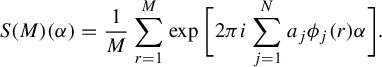 $$ \begin{align*}S(M)(\alpha)=\frac{1}{M}\sum_{r=1}^M \exp\bigg[2\pi i\sum_{j=1}^N a_j\phi_j(r) \alpha\bigg].\end{align*} $$
Observe that
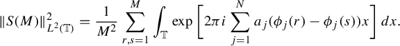 $$ \begin{align} \|S(M)\|_{L^2(\mathbb T)}^2= \frac{1}{M^2}\sum_{r,s=1}^M\int_{\mathbb T}\exp\bigg[2\pi i\sum_{j=1}^N a_j(\phi_j(r)-\phi_j(s)) x\bigg]\,dx. \end{align} $$
The right-hand side of (4.2) can be written as
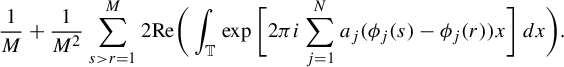 $$ \begin{align} \frac{1}{M}+\frac{1}{M^2}\sum_{s>r=1}^M2\text{Re}\bigg(\int_{\mathbb T}\exp\bigg[2\pi i\sum_{j=1}^N a_j(\phi_j(s)-\phi_j(r))x\bigg]\,dx\bigg). \end{align} $$
So, since $\phi _1,\ldots ,\phi _N$
are strongly asymptotically independent, it follows from (4.3) that for
$\phi _1,\ldots ,\phi _N$
are strongly asymptotically independent, it follows from (4.3) that for $M\in \mathbb {N}$
large enough,
$M\in \mathbb {N}$
large enough,
 $$ \begin{align*}\|S(M)\|_{L^2(\mathbb T)}^2<\frac{2}{M}.\end{align*} $$
It follows that
 $$ \begin{align*}\int_{\mathbb T} \sum_{M=1}^\infty |S(M^2)(x)|^2\,dx=\sum_{M=1}^\infty\|S(M^2)\|_{L^2(\mathbb T)}^2<\infty\end{align*} $$
and hence, for almost every $\alpha \in \mathbb T$
,
$\alpha \in \mathbb T$
, $\sum _{M=1}^\infty |S(M^2)(\alpha )|^2 <\infty $
.
$\sum _{M=1}^\infty |S(M^2)(\alpha )|^2 <\infty $
.
So, in particular, for almost every $\alpha \in \mathbb T$
,
$\alpha \in \mathbb T$
,
 $$ \begin{align} \lim_{M\rightarrow \infty} S(M^2)(\alpha)=0. \end{align} $$
We will now show that (4.4) implies that for almost every $\alpha \in \mathbb T$
,
$\alpha \in \mathbb T$
,
 $$ \begin{align*}\lim_{M\rightarrow\infty} S(M)(\alpha)=0.\end{align*} $$
Indeed, let $\alpha \in \mathbb T$
be such that
$\alpha \in \mathbb T$
be such that $\lim _{M\rightarrow \infty } S(M^2)(\alpha )=0$
and let
$\lim _{M\rightarrow \infty } S(M^2)(\alpha )=0$
and let $M,M_0\in \mathbb {N}$
satisfy
$M,M_0\in \mathbb {N}$
satisfy $M_0^2\leq M<(M_0+1)^2$
. Since
$M_0^2\leq M<(M_0+1)^2$
. Since
 $$ \begin{align*}|S(M)(\alpha)-S(M_0^2)(\alpha)| \leq \frac{1}{M_0^2}\sum_{n=1}^{M_0^2}\bigg(1-\frac{M_0^2}{M}\bigg)+\frac{1}{M}\sum_{n=M_0^2+1}^{M}1,\end{align*} $$
we have that
 $$ \begin{align*}|S(M)(\alpha)-S(M_0^2)(\alpha)|\leq 1-\frac{M_0^2}{M}+\frac{2M_0+1}{M}\leq 1-\frac{M_0^2}{(M_0+1)^2}+\frac{2M_0+1}{M_0^2}.\end{align*} $$
Thus,
 $$ \begin{align*}\lim_{M\rightarrow\infty} S(M)(\alpha)=0,\end{align*} $$
proving that $\mathfrak M_1(\phi _1,\ldots ,\phi _N)$
has full Lebesgue measure in
$\mathfrak M_1(\phi _1,\ldots ,\phi _N)$
has full Lebesgue measure in $\mathbb {R}$
.
$\mathbb {R}$
.
Now let $t\in \mathbb {N}$
and suppose that for any
$t\in \mathbb {N}$
and suppose that for any $t'\leq t$
and any strongly asymptotically independent
$t'\leq t$
and any strongly asymptotically independent $g_1,\ldots ,g_N:\mathbb {N}\rightarrow \mathbb {Z}$
,
$g_1,\ldots ,g_N:\mathbb {N}\rightarrow \mathbb {Z}$
, $\mathfrak M_{t'}(g_1,\ldots ,g_N)$
has full measure in
$\mathfrak M_{t'}(g_1,\ldots ,g_N)$
has full measure in $\mathbb {R}^{t'}$
. We want to show that
$\mathbb {R}^{t'}$
. We want to show that $\mathfrak M_{t+1}(\phi _1,\ldots ,\phi _N)$
has full measure in
$\mathfrak M_{t+1}(\phi _1,\ldots ,\phi _N)$
has full measure in $\mathbb {R}^{t+1}$
.
$\mathbb {R}^{t+1}$
.
For each $R\in \mathbb {N}$
and each
$R\in \mathbb {N}$
and each $\vec r=(r_{1,1},\ldots ,r_{N,1},\ldots ,r_{1,t},\ldots ,r_{N,t})\in \{0,\ldots , R-1\}^{Nt}$
, we define the set
$\vec r=(r_{1,1},\ldots ,r_{N,1},\ldots ,r_{1,t},\ldots ,r_{N,t})\in \{0,\ldots , R-1\}^{Nt}$
, we define the set
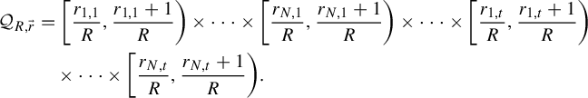 $$ \begin{align*}\mathcal Q_{R,\vec r}&=\bigg[\frac{r_{1,1}}{R},\frac{r_{1,1}+1}{R}\bigg)\times\cdots\times\bigg[\frac{r_{N,1}}{R},\frac{r_{N,1}+1}{R}\bigg)\times\cdots\times\bigg[\frac{r_{1,t}}{R},\frac{r_{1,t}+1}{R}\bigg)\\&\quad\times\cdots\times\bigg[\frac{r_{N,t}}{R},\frac{r_{N,t}+1}{R}\bigg).\end{align*} $$
Observe that for each $R\in \mathbb {N}$
,
$R\in \mathbb {N}$
, $\{\mathcal Q_{R,\vec r}\,|\,\vec r\in \{0,\ldots ,R-1\}^{Nt}\}$
is a partition of
$\{\mathcal Q_{R,\vec r}\,|\,\vec r\in \{0,\ldots ,R-1\}^{Nt}\}$
is a partition of $\mathbb T^{Nt}=[0,1)^{Nt}$
.
$\mathbb T^{Nt}=[0,1)^{Nt}$
.
Fix $(\alpha _1,\ldots ,\alpha _t)\in \mathfrak M_{t}(\phi _1,\ldots ,\phi _N)$
. For each
$(\alpha _1,\ldots ,\alpha _t)\in \mathfrak M_{t}(\phi _1,\ldots ,\phi _N)$
. For each $R\in \mathbb {N}$
and each
$R\in \mathbb {N}$
and each $\vec r\in \{0,\ldots ,R-1\}^{Nt}$
, let
$\vec r\in \{0,\ldots ,R-1\}^{Nt}$
, let $(n_k^{(R,\vec r)})_{k\in \mathbb {N}}$
be the unique increasing sequence satisfying
$(n_k^{(R,\vec r)})_{k\in \mathbb {N}}$
be the unique increasing sequence satisfying
 $$ \begin{align*}&\{n^{(R,\vec r)}_k\,|\,k\in\mathbb{N}\}\\&\quad=\{n\in\mathbb{N}\,|\,(\phi_1(n)\alpha_1,\ldots,\phi_N(n)\alpha_1,\ldots,\phi_1(n)\alpha_t,\ldots,\phi_N(n)\alpha_t)\text{ mod }1\in\mathcal Q_{R,\vec r}\}.\end{align*} $$
For each $j\in \{1,\ldots ,N\}$
, let
$j\in \{1,\ldots ,N\}$
, let $\phi _j^{(R,\vec r)}:\mathbb {N}\rightarrow \mathbb {Z}$
be defined by
$\phi _j^{(R,\vec r)}:\mathbb {N}\rightarrow \mathbb {Z}$
be defined by
 $$ \begin{align*}\phi_j^{(R,\vec r)}(k)=\phi_j(n^{(R,\vec r)}_k).\end{align*} $$
(Observe that since $\phi _1^{(R,\vec r)}$
,…,
$\phi _1^{(R,\vec r)}$
,…, $\phi _N^{(R,\vec r)}$
are ‘simultaneous’ subsequences of
$\phi _N^{(R,\vec r)}$
are ‘simultaneous’ subsequences of $\phi _1,\ldots ,\phi _N$
, the sequences
$\phi _1,\ldots ,\phi _N$
, the sequences $\phi _1^{(R,\vec r)}$
,…,
$\phi _1^{(R,\vec r)}$
,…, $\phi _N^{(R,\vec r)}$
are strongly asymptotically independent.)
$\phi _N^{(R,\vec r)}$
are strongly asymptotically independent.)
Let
 $$ \begin{align*}\mathfrak M'(\phi_1,\ldots,\phi_N,\alpha_1,\ldots,\alpha_t)=\bigcap_{R\in\mathbb{N}}\bigcap_{\vec r\in\{0,\ldots,R-1\}^{Nt}} \mathfrak M_1(\phi_1^{(R,\vec r)},\ldots,\phi_N^{(R,\vec r)}).\end{align*} $$
Note that by the inductive hypothesis, $\mathfrak M'(\phi _1,\ldots ,\phi _N,\alpha _1,\ldots ,\alpha _t)$
has full measure in
$\mathfrak M'(\phi _1,\ldots ,\phi _N,\alpha _1,\ldots ,\alpha _t)$
has full measure in $\mathbb {R}$
. Pick
$\mathbb {R}$
. Pick $\alpha \in \mathfrak M'(\phi _1,\ldots ,\phi _N,\alpha _1,\ldots ,\alpha _t)$
. For any
$\alpha \in \mathfrak M'(\phi _1,\ldots ,\phi _N,\alpha _1,\ldots ,\alpha _t)$
. For any $(a_{1,1},\ldots ,a_{N,1},\ldots ,a_{1,t},\ldots , a_{N,t}) \in \mathbb {Z}^{Nt}$
and any
$(a_{1,1},\ldots ,a_{N,1},\ldots ,a_{1,t},\ldots , a_{N,t}) \in \mathbb {Z}^{Nt}$
and any $(a_1,\ldots ,a_N)\in \mathbb {Z}^N\setminus \{\vec 0\}$
,
$(a_1,\ldots ,a_N)\in \mathbb {Z}^N\setminus \{\vec 0\}$
,
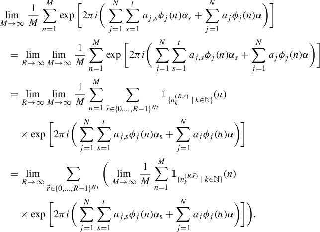
Fix $R\in \mathbb {N}$
and
$R\in \mathbb {N}$
and $\vec r\in \{0,\ldots ,R-1\}^{Nt}$
. By our choice of
$\vec r\in \{0,\ldots ,R-1\}^{Nt}$
. By our choice of $(\alpha _1,\ldots ,\alpha _t)$
and the definition of
$(\alpha _1,\ldots ,\alpha _t)$
and the definition of $(n_k^{(R,\vec r)})_{k\in \mathbb {N}}$
,
$(n_k^{(R,\vec r)})_{k\in \mathbb {N}}$
,
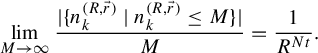 $$ \begin{align*}\lim_{M\rightarrow\infty}\frac{|\{n_k^{(R,\vec r)}\,|\,n_k^{(R,\vec r)}\leq M\}|}{M}=\frac{1}{R^{Nt}}.\end{align*} $$
So,
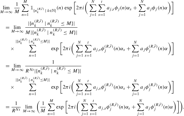
Observe that for any $\epsilon>0$
, there exists an
$\epsilon>0$
, there exists an $R_0\in \mathbb {N}$
such that for any
$R_0\in \mathbb {N}$
such that for any $R\geq R_0$
, any
$R\geq R_0$
, any $\vec r\in \{0,\ldots ,R-1\}^{Nt},$
and any
$\vec r\in \{0,\ldots ,R-1\}^{Nt},$
and any $n\in \mathbb {N}$
,
$n\in \mathbb {N}$
,
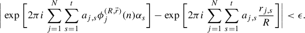 $$ \begin{align*}\bigg|\exp\bigg[2\pi i\sum_{j=1}^N\sum_{s=1}^ta_{j,s}\phi^{(R,\vec r)}_j(n)\alpha_s\bigg]-\exp\bigg[2\pi i\sum_{j=1}^N\sum_{s=1}^ta_{j,s}\frac{r_{j,s}}{R}\bigg]\bigg|<\epsilon.\end{align*} $$
It follows from (4.5) that
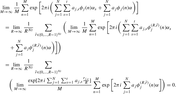 $$ \begin{align*} &\lim_{M\rightarrow\infty}\frac{1}{M}\sum_{n=1}^M\exp\bigg[2\pi i\bigg(\sum_{j=1}^N\sum_{s=1}^ta_{j,s}\phi_j(n)\alpha_s+\sum_{j=1}^Na_j\phi_j(n)\alpha\bigg)\bigg]\\ &\quad=\lim_{R\rightarrow\infty}\frac{1}{R^{Nt}}\sum_{\vec r\in\{0,\ldots,R-1\}^{Nt}}\bigg(\lim_{M\rightarrow\infty}\frac{1}{M} \sum_{n=1}^{M}\exp\bigg[2\pi i\bigg(\sum_{j=1}^N\sum_{s=1}^ta_{j,s}\phi^{(R,\vec r)}_j(n)\alpha_s\\&\qquad+\sum_{j=1}^Na_j\phi^{(R,\vec r)}_j(n)\alpha\bigg)\bigg]\bigg)\\ &\quad=\lim_{R\rightarrow\infty}\frac{1}{R^{Nt}}\sum_{\vec r\in\{0,\ldots,R-1\}^{Nt}}\\&\qquad\bigg(\lim_{M\rightarrow\infty}\frac{\exp[2\pi i\sum_{j=1}^N\sum_{s=1}^ta_{j,s}\frac{r_{j,s}}{R}]}{M} \sum_{n=1}^{M}\exp\bigg[2\pi i\sum_{j=1}^Na_j\phi^{(R,\vec r)}_j(n)\alpha\bigg]\bigg)=0. \end{align*} $$
So $(\alpha _1,\ldots ,\alpha _t,\alpha )\in \mathfrak M_{t+1}(\phi _1,\ldots ,\phi _N)$
.
$(\alpha _1,\ldots ,\alpha _t,\alpha )\in \mathfrak M_{t+1}(\phi _1,\ldots ,\phi _N)$
.
Since $\mathfrak M_t(\phi _1,\ldots ,\phi _N)$
has full measure and for any
$\mathfrak M_t(\phi _1,\ldots ,\phi _N)$
has full measure and for any $(\alpha _1,\ldots ,\alpha _t)\in \mathfrak M_t(\phi _1,\ldots ,\phi _N)$
,
$(\alpha _1,\ldots ,\alpha _t)\in \mathfrak M_t(\phi _1,\ldots ,\phi _N)$
, $\mathfrak M'(\phi _1,\ldots ,\phi _N,\alpha _1,\ldots ,\alpha _t)$
also has full measure, Fubini’s theorem implies that
$\mathfrak M'(\phi _1,\ldots ,\phi _N,\alpha _1,\ldots ,\alpha _t)$
also has full measure, Fubini’s theorem implies that $\mathfrak M_{t+1}(\phi _1,\ldots ,\phi _N)$
has full measure. This completes the induction.
$\mathfrak M_{t+1}(\phi _1,\ldots ,\phi _N)$
has full measure. This completes the induction.
To see that for any $(\alpha _1,\ldots ,\alpha _t)\in \mathfrak M_t(\phi _1,\ldots ,\phi _N)$
,
$(\alpha _1,\ldots ,\alpha _t)\in \mathfrak M_t(\phi _1,\ldots ,\phi _N)$
, $\mathfrak M(\phi _1,\ldots ,\phi _N,\alpha _1,\ldots ,\alpha _t)$
has full measure, simply note that
$\mathfrak M(\phi _1,\ldots ,\phi _N,\alpha _1,\ldots ,\alpha _t)$
has full measure, simply note that
 $$ \begin{align*}\mathfrak M'(\phi_1,\ldots,\phi_N,\alpha_1,\ldots,\alpha_t)\subseteq \mathfrak M(\phi_1,\ldots,\phi_N,\alpha_1,\ldots,\alpha_t).\\[-3.3pc]\end{align*} $$
Theorem 4.2. Let $N\in \mathbb {N}$
and let
$N\in \mathbb {N}$
and let $\phi _1,\ldots ,\phi _N:\mathbb {N}\rightarrow \mathbb {Z}$
be asymptotically independent sequences. Then there exists an increasing sequence
$\phi _1,\ldots ,\phi _N:\mathbb {N}\rightarrow \mathbb {Z}$
be asymptotically independent sequences. Then there exists an increasing sequence $(n_k)_{k\in \mathbb {N}}$
in
$(n_k)_{k\in \mathbb {N}}$
in $\mathbb {N}$
such that for any
$\mathbb {N}$
such that for any $\vec \xi =(\xi _1,\ldots ,\xi _N)\in \{0,1\}^N$
, there exists a non-trivial weakly mixing Gaussian system
$\vec \xi =(\xi _1,\ldots ,\xi _N)\in \{0,1\}^N$
, there exists a non-trivial weakly mixing Gaussian system $(\mathbb {R}^{\mathbb {Z}},\mathcal A,\gamma _{\vec \xi },T_{\vec \xi })$
with the property that for each
$(\mathbb {R}^{\mathbb {Z}},\mathcal A,\gamma _{\vec \xi },T_{\vec \xi })$
with the property that for each $j\in \{1,\ldots ,N\}$
and any
$j\in \{1,\ldots ,N\}$
and any $A,B\in \mathcal A$
,
$A,B\in \mathcal A$
,
 $$ \begin{align} \lim_{k\rightarrow\infty}\gamma_{\kern1.5pt\vec\xi}(A\cap T_{\vec \xi}^{-\phi_j(n_k)}B)=(1-\xi_j)\gamma_{\kern1.5pt\vec\xi}(A\cap B)+\xi_j\gamma_{\kern1.5pt\vec\xi}(A)\gamma_{\kern1.5pt\vec\xi}(B). \end{align} $$
Proof. As in the proof of Theorem 3.1, we will construct spectral measures $\sigma _{\vec \xi }$
,
$\sigma _{\vec \xi }$
, $\vec \xi \in \{0,1\}^N$
, which have associated Gaussian systems with the desired properties. For each
$\vec \xi \in \{0,1\}^N$
, which have associated Gaussian systems with the desired properties. For each $\vec \xi =(\xi _1,\ldots ,\xi _N) \in \{0,1\}^N$
, let
$\vec \xi =(\xi _1,\ldots ,\xi _N) \in \{0,1\}^N$
, let $\vec b_{\vec \xi }=(b_1^{(\vec \xi )},\ldots ,b_N^{(\vec \xi )})\in \mathbb {Q}^N$
be defined as in (3.5) (so
$\vec b_{\vec \xi }=(b_1^{(\vec \xi )},\ldots ,b_N^{(\vec \xi )})\in \mathbb {Q}^N$
be defined as in (3.5) (so $b^{(\vec \xi )}_j=1-{\xi _j}/{2}$
for each
$b^{(\vec \xi )}_j=1-{\xi _j}/{2}$
for each $j\in \{1,\ldots ,N\}$
) and for each
$j\in \{1,\ldots ,N\}$
) and for each $k\in \mathbb {N}$
, let
$k\in \mathbb {N}$
, let
 $$ \begin{align*}\Phi(k)=\max_{j\in\{1,\ldots,N\}}|\phi_j(k)|+1.\end{align*} $$
We claim that there exist: (a) an increasing sequence $(n_k)_{k\in \mathbb {N}}$
in
$(n_k)_{k\in \mathbb {N}}$
in $\mathbb {N}$
and (b) sequences of irrational numbers
$\mathbb {N}$
and (b) sequences of irrational numbers $(\alpha _k^{(\vec \xi )})_{k\in \mathbb {N}}$
,
$(\alpha _k^{(\vec \xi )})_{k\in \mathbb {N}}$
, $\vec \xi \in \{0,1\}^N$
, which satisfy the following conditions.
$\vec \xi \in \{0,1\}^N$
, which satisfy the following conditions.
(1) For each $k\in \mathbb {N}$
and each
$k\in \mathbb {N}$
and each $\vec \xi \in \{0,1\}^N$
,
$\vec \xi \in \{0,1\}^N$
, $\alpha _{k}^{(\vec \xi )}\in (0,{1}/[{2^{k}\Phi (n_{k-1})}]$
, where
$\alpha _{k}^{(\vec \xi )}\in (0,{1}/[{2^{k}\Phi (n_{k-1})}]$
, where $n_0=1$
. So, in particular,
$n_0=1$
. So, in particular,
 $$ \begin{align*}\lim_{t\rightarrow\infty}\phi_\ell(n_t)\sum_{s=t+1}^\infty \bigg|\frac{\alpha_s^{(\vec \xi)}}{2}\bigg|=0\end{align*} $$
for each $\ell \in \{1,\ldots ,N\}$
.
$\ell \in \{1,\ldots ,N\}$
.
(2) For each $k\in \mathbb {N}$
, each
$k\in \mathbb {N}$
, each $\vec \xi \in \{0,1\}^N$
, and each
$\vec \xi \in \{0,1\}^N$
, and each $\ell \in \{1,\ldots ,N\}$
,
$\ell \in \{1,\ldots ,N\}$
,
 $$ \begin{align*}\bigg\|\phi_\ell(n_k)\frac{\alpha_k^{(\vec \xi)}}{2}-\frac{b^{(\vec \xi)}_\ell}{2}\bigg\|<\frac{1}{k},\end{align*} $$
which implies
 $$ \begin{align*}\lim_{t\rightarrow\infty}\bigg\|\phi_\ell(n_t)\frac{\alpha_t^{(\vec \xi)}}{2}- \frac{b^{(\vec \xi)}_\ell}{2}\bigg\|=0.\end{align*} $$
(3) For each $k\in \mathbb {N}$
, each
$k\in \mathbb {N}$
, each $\vec \xi \in \{0,1\}^N$
, each
$\vec \xi \in \{0,1\}^N$
, each $\ell \in \{1,\ldots ,N\}$
, and each
$\ell \in \{1,\ldots ,N\}$
, and each $k_0\in \mathbb {N}$
with
$k_0\in \mathbb {N}$
with $k_0<k$
,
$k_0<k$
,
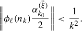 $$ \begin{align*}\bigg\|\phi_\ell(n_k)\frac{\alpha_{k_0}^{(\vec \xi)}}{2}\bigg\|<\frac{1}{k^2}.\end{align*} $$
This means that
 $$ \begin{align*}\lim_{k\rightarrow\infty}\bigg\|\phi_\ell(n_k)\frac{\alpha_{k_0}^{(\vec \xi)}}{2}\bigg\|=0\end{align*} $$
fast enough to ensure that
 $$ \begin{align*}\lim_{k\rightarrow\infty}\sum_{t=1}^k\bigg\|\phi_\ell(n_{k+1})\frac{\alpha_t^{(\vec \xi)}}{2}\bigg\|=0.\end{align*} $$
Indeed, we define the sequences $(n_k)_{k\in \mathbb {N}}$
and
$(n_k)_{k\in \mathbb {N}}$
and $(\alpha _k^{(\vec \xi )})_{k\in \mathbb {N}}$
,
$(\alpha _k^{(\vec \xi )})_{k\in \mathbb {N}}$
, $\vec \xi \in \{0,1\}^N$
, inductively on
$\vec \xi \in \{0,1\}^N$
, inductively on $k\in \mathbb {N}$
. First, note that there exists an increasing sequence
$k\in \mathbb {N}$
. First, note that there exists an increasing sequence $(m_k)_{k\in \mathbb {N}}$
in
$(m_k)_{k\in \mathbb {N}}$
in $\mathbb {N}$
for which the sequences
$\mathbb {N}$
for which the sequences
 $$ \begin{align*}\psi_j(k)=\phi_j(m_k),\quad j\in\{1,\ldots,N\}\end{align*} $$
are strongly asymptotically independent. Let $\vec \xi _1,\ldots ,\vec \xi _{2^N}$
be an enumeration of
$\vec \xi _1,\ldots ,\vec \xi _{2^N}$
be an enumeration of $\{0,1\}^N$
. To construct the desired sequences, we will need to show that the sequences
$\{0,1\}^N$
. To construct the desired sequences, we will need to show that the sequences $(\alpha _k^{(\vec \xi )})_{k\in \mathbb {N}}$
,
$(\alpha _k^{(\vec \xi )})_{k\in \mathbb {N}}$
, $\vec \xi \in \{0,1\}^N$
, satisfy the following additional property.
$\vec \xi \in \{0,1\}^N$
, satisfy the following additional property.
(4) For any $k\in \mathbb {N}$
, the sequence
$k\in \mathbb {N}$
, the sequence
 $$ \begin{align*} &(\phi_1(m_t)\alpha_1^{(\vec \xi_1)},\ldots,\phi_N(m_t)\alpha_1^{(\vec \xi_1)},\ldots, \phi_1(m_t)\alpha_{1}^{(\vec \xi_{2^N})},\ldots,\phi_N(m_t)\alpha_{1}^{(\vec \xi_{2^N})},\\ & \qquad\qquad\qquad\qquad\qquad\qquad\qquad \vdots\\ & \phi_1(m_t)\alpha_k^{(\vec \xi_1)},\ldots,\phi_N(m_t)\alpha_k^{(\vec \xi_1)},\ldots, \phi_1(m_t)\alpha_{k}^{(\vec \xi_{2^N})},\ldots,\phi_N(m_t)\alpha_{k}^{(\vec \xi_{2^N})} ),\,t\in\mathbb{N} \end{align*} $$
is uniformly distributed $\mod \!1$
.
$\mod \!1$
.
By Lemma 4.1, we can pick
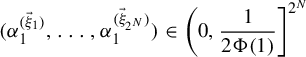 $$ \begin{align*}(\alpha_1^{(\vec \xi_1)},\ldots,\alpha_{1}^{(\vec \xi_{2^N})})\in \bigg(0,\frac{1}{2\Phi(1)}\bigg]^{2^N}\end{align*} $$
such that the sequence
 $$ \begin{align*}(\phi_1(m_t)\alpha_1^{(\vec \xi_1)},\ldots,\phi_N(m_t)\alpha_1^{(\vec \xi_1)},\ldots, \phi_1(m_t)\alpha_{1}^{(\vec \xi_{2^N})},\ldots,\phi_N(m_t)\alpha_{1}^{(\vec \xi_{2^N})}),\quad t\in\mathbb{N}\end{align*} $$
is uniformly distributed $\, \mod \!1$
(and so,
$\, \mod \!1$
(and so, $\alpha _1^{(\vec \xi _1)},\ldots ,\alpha _{1}^{(\vec \xi _{2^N})}$
satisfy (4)). Pick
$\alpha _1^{(\vec \xi _1)},\ldots ,\alpha _{1}^{(\vec \xi _{2^N})}$
satisfy (4)). Pick $t_1\in \mathbb {N}$
arbitrarily. Setting
$t_1\in \mathbb {N}$
arbitrarily. Setting $n_1=m_{t_1}$
, one can check that
$n_1=m_{t_1}$
, one can check that $n_1$
and
$n_1$
and $\alpha _{1}^{(\vec \xi _1)}$
, …,
$\alpha _{1}^{(\vec \xi _1)}$
, …, $\alpha _{1}^{(\vec \xi _{2^N})}$
satisfy conditions (1), (2), and (3) (note that for
$\alpha _{1}^{(\vec \xi _{2^N})}$
satisfy conditions (1), (2), and (3) (note that for $k=1$
, condition (2) is trivial and condition (3) is vacuous).
$k=1$
, condition (2) is trivial and condition (3) is vacuous).
Fix now $k\in \mathbb {N}$
and suppose we have chosen
$k\in \mathbb {N}$
and suppose we have chosen $\alpha _{1}^{(\vec \xi )},\ldots ,\alpha _{k}^{(\vec \xi )}$
,
$\alpha _{1}^{(\vec \xi )},\ldots ,\alpha _{k}^{(\vec \xi )}$
, $\vec \xi \in \{0,1\}^N$
, and
$\vec \xi \in \{0,1\}^N$
, and $n_1<\cdots <n_k$
satisfying conditions (1)–(4). Note that
$n_1<\cdots <n_k$
satisfying conditions (1)–(4). Note that $(0,{1}/[{2^{k+1}\Phi (n_{k})}]$
has positive measure. By repeatedly applying (4.1) in Lemma 4.1, we can find
$(0,{1}/[{2^{k+1}\Phi (n_{k})}]$
has positive measure. By repeatedly applying (4.1) in Lemma 4.1, we can find
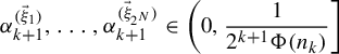 $$ \begin{align*}\alpha_{k+1}^{(\vec \xi_1)},\ldots,\alpha_{k+1}^{(\vec \xi_{2^N})}\in \bigg(0,\frac{1}{2^{k+1}\Phi(n_{k})}\bigg]\end{align*} $$
such that for each $s\in \{1,\ldots ,2^N\}$
, the sequence
$s\in \{1,\ldots ,2^N\}$
, the sequence
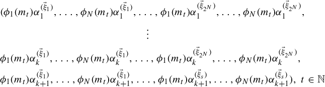 $$ \begin{align*} &(\phi_1(m_t)\alpha_1^{(\vec \xi_1)},\ldots,\phi_N(m_t)\alpha_1^{(\vec \xi_1)},\ldots, \phi_1(m_t)\alpha_{1}^{(\vec \xi_{2^N})},\ldots,\phi_N(m_t)\alpha_{1}^{(\vec \xi_{2^N})},\\ & \qquad\qquad\qquad\qquad\qquad\qquad\qquad \vdots\\ & \phi_1(m_t)\alpha_k^{(\vec \xi_1)},\ldots,\phi_N(m_t)\alpha_k^{(\vec \xi_1)},\ldots, \phi_1(m_t)\alpha_{k}^{(\vec \xi_{2^N})},\ldots,\phi_N(m_t)\alpha_{k}^{(\vec \xi_{2^N})},\\ & \phi_1(m_t)\alpha_{k+1}^{(\vec \xi_1)},\ldots,\phi_N(m_t)\alpha_{k+1}^{(\vec \xi_{1})},\ldots,\phi_1(m_t)\alpha_{k+1}^{(\vec \xi_s)},\ldots,\phi_N(m_t)\alpha_{k+1}^{(\vec \xi_{s})} ),\,t\in\mathbb{N} \end{align*} $$
is uniformly distributed $\, \mod \!1$
. It follows that
$\, \mod \!1$
. It follows that $\alpha _1^{(\vec \xi )},\ldots ,\alpha _{k+1}^{(\vec \xi )}$
,
$\alpha _1^{(\vec \xi )},\ldots ,\alpha _{k+1}^{(\vec \xi )}$
, $\vec \xi \in \{0,1\}^N$
, satisfy condition (4) and hence one can find
$\vec \xi \in \{0,1\}^N$
, satisfy condition (4) and hence one can find $t_{k+1}\in \mathbb {N}$
for which conditions (1)–(3) hold for
$t_{k+1}\in \mathbb {N}$
for which conditions (1)–(3) hold for $n_{k+1}=m_{t_{k+1}}$
and
$n_{k+1}=m_{t_{k+1}}$
and $n_k<n_{k+1}$
, completing the induction.
$n_k<n_{k+1}$
, completing the induction.
Fix $\vec \xi =(\xi _1,\ldots ,\xi _N)\in \{0,1\}^N$
. By conditions (1)–(3), for any
$\vec \xi =(\xi _1,\ldots ,\xi _N)\in \{0,1\}^N$
. By conditions (1)–(3), for any $\epsilon>0$
, there exists
$\epsilon>0$
, there exists $k_\epsilon \in \mathbb {N}$
such that for any
$k_\epsilon \in \mathbb {N}$
such that for any $k>k_\epsilon $
, any
$k>k_\epsilon $
, any $\ell \in \{1,\ldots ,N\}$
, and any
$\ell \in \{1,\ldots ,N\}$
, and any $\omega \in \{0,1\}^{\mathbb {N}}$
,
$\omega \in \{0,1\}^{\mathbb {N}}$
,
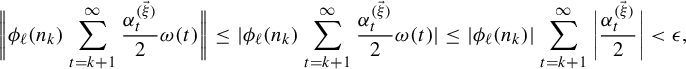 $$ \begin{align} \bigg\|\phi_\ell(n_k)\sum_{t=k+1}^\infty\frac{\alpha^{(\vec \xi)}_t}{2}\omega(t)\bigg\|\leq| \phi_\ell(n_k)\sum_{t=k+1}^\infty\frac{\alpha^{(\vec \xi)}_t}{2}\omega(t)|\leq |\phi_\ell(n_k)|\sum_{t=k+1}^\infty\bigg|\frac{\alpha^{(\vec \xi)}_t}{2}\bigg|<\epsilon, \end{align} $$
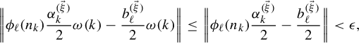 $$ \begin{align} \bigg\|\phi_\ell(n_k)\frac{\alpha_k^{(\vec \xi)}}{2}\omega(k)-\frac{b^{(\vec \xi)}_\ell}{2}\omega(k)\bigg\|\leq \bigg\|\phi_\ell(n_k)\frac{\alpha_k^{(\vec \xi)}}{2}-\frac{b^{(\vec \xi)}_\ell}{2}\bigg\|<\epsilon, \end{align} $$
and
 $$ \begin{align} \bigg\|\phi_\ell(n_k)\sum_{t=1}^{k-1}\frac{\alpha_t^{(\vec \xi)}}{2}\omega(t)\bigg\| \leq \sum_{t=1}^{k-1}\bigg\|\phi_\ell(n_k)\frac{\alpha_t^{(\vec \xi)}}{2}\bigg\|<\epsilon. \end{align} $$
Let $f:\{0,1\}^{\mathbb {N}}\rightarrow \mathbb {R}$
be defined by
$f:\{0,1\}^{\mathbb {N}}\rightarrow \mathbb {R}$
be defined by
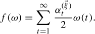 $$ \begin{align*}f(\omega)=\sum_{t=1}^\infty \frac{\alpha^{(\vec \xi)}_t}{2}\omega(t).\end{align*} $$
Combining (4.7), (4.8), and (4.9), one has that for any $\epsilon>0$
, there exists a
$\epsilon>0$
, there exists a $k_\epsilon \in \mathbb {N}$
such that for any
$k_\epsilon \in \mathbb {N}$
such that for any $k>k_\epsilon $
, any
$k>k_\epsilon $
, any $\ell \in \{1,\ldots ,N\}$
, and any
$\ell \in \{1,\ldots ,N\}$
, and any $\omega \in \{0,1\}^{\mathbb {N}}$
,
$\omega \in \{0,1\}^{\mathbb {N}}$
,
 $$ \begin{align} \bigg\|\phi_\ell(n_k)f(\omega)- \frac{b_\ell^{(\vec \xi)}}{2}\omega(k)\bigg\|<\epsilon. \end{align} $$
Let now $f_{\vec \xi }:\{0,1\}^{\mathbb {N}}\times \{0,1\}^{\mathbb {N}}\rightarrow \mathbb T$
be defined by
$f_{\vec \xi }:\{0,1\}^{\mathbb {N}}\times \{0,1\}^{\mathbb {N}}\rightarrow \mathbb T$
be defined by
 $$ \begin{align*}f_{\vec \xi}(\omega_1,\omega_2)=2(f(\omega_1)-f(\omega_2))\,\text{mod}\,1=\sum_{t=1}^\infty \alpha_t^{(\vec \xi)}(\omega_1(t)-\omega_2(t))\,\text{mod}\,1.\end{align*} $$
Setting $\sigma _{\vec \xi }=(\mathbb P\times \mathbb P)\circ f_{\vec \xi }^{-1}$
and imitating the proof of Theorem 3.1, we obtain the desired result.
$\sigma _{\vec \xi }=(\mathbb P\times \mathbb P)\circ f_{\vec \xi }^{-1}$
and imitating the proof of Theorem 3.1, we obtain the desired result.
Corollary 4.3. Let $N\in \mathbb {N}$
and let
$N\in \mathbb {N}$
and let $t\in \{0,\ldots ,N\}$
. For any
$t\in \{0,\ldots ,N\}$
. For any $a_1,\ldots ,a_N\in \mathbb {Z}$
and any linearly independent polynomials
$a_1,\ldots ,a_N\in \mathbb {Z}$
and any linearly independent polynomials $v_1,\ldots ,v_N\in \mathbb {Z}[x]$
with
$v_1,\ldots ,v_N\in \mathbb {Z}[x]$
with $v_j(0)=0$
for each
$v_j(0)=0$
for each $j\in \{1,\ldots ,N\}$
, there exists a weakly mixing Gaussian system
$j\in \{1,\ldots ,N\}$
, there exists a weakly mixing Gaussian system $(\mathbb {R}^{\mathbb {Z}},\mathcal A,\gamma , T)$
and an increasing sequence
$(\mathbb {R}^{\mathbb {Z}},\mathcal A,\gamma , T)$
and an increasing sequence $(n_k)_{k\in \mathbb {N}}$
in
$(n_k)_{k\in \mathbb {N}}$
in $\mathbb {N}$
such that for any
$\mathbb {N}$
such that for any $A,B\in \mathcal A$
,
$A,B\in \mathcal A$
,
 $$ \begin{align*}\lim_{k\rightarrow\infty}\gamma(A\cap T^{- v_j(n_k)}B)=\begin{cases} \gamma(A\cap T^{-a_j} B)&\text{if }j\leq t,\\ \gamma(A)\gamma(B)&\text{if }j\in\{1,\ldots,N\}\setminus\{0,\ldots,t\}. \end{cases}\end{align*} $$
Proof. For each $j\in \{0,\ldots ,t\}\setminus \{0\}$
, let
$j\in \{0,\ldots ,t\}\setminus \{0\}$
, let $(\phi _j(k))_{k\in \mathbb {N}}=(v_j(k)-a_j)_{k\in \mathbb {N}}$
and for each
$(\phi _j(k))_{k\in \mathbb {N}}=(v_j(k)-a_j)_{k\in \mathbb {N}}$
and for each $j\in \{1,\ldots ,N\}\setminus \{0,\ldots ,t\}$
, let
$j\in \{1,\ldots ,N\}\setminus \{0,\ldots ,t\}$
, let $(\phi _j(k))_{k\in \mathbb {N}}=(v_j(k))_{k\in \mathbb {N}}$
. The result now follows by applying Theorem 4.2 to the asymptotically independent sequences
$(\phi _j(k))_{k\in \mathbb {N}}=(v_j(k))_{k\in \mathbb {N}}$
. The result now follows by applying Theorem 4.2 to the asymptotically independent sequences $\phi _1,\ldots ,\phi _N$
.
$\phi _1,\ldots ,\phi _N$
.
5 Interpolating between rigidity and mixing
Our goal in this section is to prove Theorem 1.3 and obtain Theorem 1.2 as a corollary. We now restate Theorem 1.3. (Recall that we denote by $\mathbb {N}^{\mathbb {N}}_\infty $
the set of all (strictly) increasing sequences
$\mathbb {N}^{\mathbb {N}}_\infty $
the set of all (strictly) increasing sequences $(n_k)_{k\in \mathbb {N}}$
in
$(n_k)_{k\in \mathbb {N}}$
in $\mathbb {N}$
.)
$\mathbb {N}$
.)
Theorem 5.1. Let $N\in \mathbb {N}$
, let
$N\in \mathbb {N}$
, let $\unicode{x3bb} _1,\ldots ,\unicode{x3bb} _N\in [0,1]$
, and let
$\unicode{x3bb} _1,\ldots ,\unicode{x3bb} _N\in [0,1]$
, and let $\phi _1,\ldots ,\phi _N:\mathbb {N}\rightarrow \mathbb {Z}$
. Suppose that
$\phi _1,\ldots ,\phi _N:\mathbb {N}\rightarrow \mathbb {Z}$
. Suppose that $\phi _1,\ldots ,\phi _N$
satisfy the following condition.
$\phi _1,\ldots ,\phi _N$
satisfy the following condition.
Condition C: There exists an $(n_k)_{k\in \mathbb {N}}\in \mathbb {N}^{\mathbb {N}}_\infty $
such that for any
$(n_k)_{k\in \mathbb {N}}\in \mathbb {N}^{\mathbb {N}}_\infty $
such that for any $\vec \xi =(\xi _1,\ldots ,\xi _N)\in \{0,1\}^N$
, there exists an aperiodic
$\vec \xi =(\xi _1,\ldots ,\xi _N)\in \{0,1\}^N$
, there exists an aperiodic $T_{\vec \xi }\in \operatorname {Aut}([0,1],\mathcal B,\mu )$
with the property that for each
$T_{\vec \xi }\in \operatorname {Aut}([0,1],\mathcal B,\mu )$
with the property that for each $j\in \{1,\ldots ,N\}$
and any
$j\in \{1,\ldots ,N\}$
and any $A,B\in \mathcal B$
,
$A,B\in \mathcal B$
,
 $$ \begin{align*} \lim_{k\rightarrow\infty}\mu(A\cap T_{\vec \xi}^{- \phi_j(n_k)}B)=(1-\xi_j)\mu(A\cap B)+\xi_j\mu(A)\mu(B). \end{align*} $$
Then the set
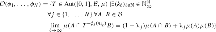
is a dense $G_{\!\delta }$
set.
$G_{\!\delta }$
set.
Before proving Theorem 5.1, we will review the necessary background material on $\operatorname {Aut}([0,1],\mathcal B,\mu )$
.
$\operatorname {Aut}([0,1],\mathcal B,\mu )$
.
5.1 Background on
$\operatorname {Aut}([0,1],\mathcal B,\mu )$

We will follow the material and the terminology in [Reference Halmos7]. For each $\ell \in \mathbb {N}$
, let
$\ell \in \mathbb {N}$
, let $E_\ell $
denote the family of the half-open intervals
$E_\ell $
denote the family of the half-open intervals
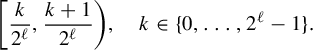 $$ \begin{align*}\bigg[\frac{k}{2^\ell},\frac{k+1}{2^\ell}\bigg),\quad k\in\{0,\ldots,2^\ell-1\}.\end{align*} $$
We call each element of $E_\ell $
a dyadic interval of rank
$E_\ell $
a dyadic interval of rank $\ell $
. Define the metric
$\ell $
. Define the metric $\partial $
on
$\partial $
on $\operatorname {Aut}([0,1],\mathcal B,\mu )$
by
$\operatorname {Aut}([0,1],\mathcal B,\mu )$
by
 $$ \begin{align} \partial(T,S)=\sum_{\ell\in\mathbb{N}}\frac{1}{2^{2\ell}}\sum_{E \in E_\ell}\mu(T E\triangle S E), \end{align} $$
where $T E\triangle S E$
denotes the symmetric difference between the sets
$T E\triangle S E$
denotes the symmetric difference between the sets $TE$
and
$TE$
and $SE$
. The topology induced by
$SE$
. The topology induced by $\partial $
is called the weak topology of
$\partial $
is called the weak topology of $\operatorname {Aut}([0,1],\mathcal B,\mu )$
.
$\operatorname {Aut}([0,1],\mathcal B,\mu )$
.
With this topology, a sequence $(T_k)_{k\in \mathbb {N}}$
in
$(T_k)_{k\in \mathbb {N}}$
in $\operatorname {Aut}([0,1],\mathcal B,\mu )$
converges to
$\operatorname {Aut}([0,1],\mathcal B,\mu )$
converges to $T\in \operatorname {Aut}([0,1],\mathcal B,\mu )$
if and only if
$T\in \operatorname {Aut}([0,1],\mathcal B,\mu )$
if and only if $(T_k)_{k\in \mathbb {N}}$
converges to T with respect to the weak operator topology on
$(T_k)_{k\in \mathbb {N}}$
converges to T with respect to the weak operator topology on $L^2(\mu )$
if and only if
$L^2(\mu )$
if and only if $(T_k)_{k\in \mathbb {N}}$
converges to T in the strong operator topology on
$(T_k)_{k\in \mathbb {N}}$
converges to T in the strong operator topology on $L^2(\mu )$
. Furthermore,
$L^2(\mu )$
. Furthermore, $(\operatorname {Aut}([0,1],\mathcal B,\mu ),\partial )$
is a topological group.
$(\operatorname {Aut}([0,1],\mathcal B,\mu ),\partial )$
is a topological group.
We remark that while $\operatorname {Aut}([0,1],\mathcal B,\mu )$
with the weak topology is completely metrizable, the metric space
$\operatorname {Aut}([0,1],\mathcal B,\mu )$
with the weak topology is completely metrizable, the metric space $(\operatorname {Aut}([0,1],\mathcal B,\mu ),\partial )$
is not complete (that is, not every Cauchy sequence needs to be convergent).
$(\operatorname {Aut}([0,1],\mathcal B,\mu ),\partial )$
is not complete (that is, not every Cauchy sequence needs to be convergent).
We now turn our attention to some of the dense subsets of $(\operatorname {Aut}([0,1],\mathcal B,\mu ),\partial )$
. Given
$(\operatorname {Aut}([0,1],\mathcal B,\mu ),\partial )$
. Given $\ell \in \mathbb {N}$
, a transformation
$\ell \in \mathbb {N}$
, a transformation $T\in \operatorname {Aut}([0,1],\mathcal B,\mu )$
is a cyclic permutation of the dyadic intervals of rank
$T\in \operatorname {Aut}([0,1],\mathcal B,\mu )$
is a cyclic permutation of the dyadic intervals of rank $\ell $
if for any
$\ell $
if for any $E\in E_\ell $
: (a)
$E\in E_\ell $
: (a) $TE\in E_\ell $
; (b) there exists an
$TE\in E_\ell $
; (b) there exists an $\alpha \in \mathbb {R}$
such that for any
$\alpha \in \mathbb {R}$
such that for any $x\in E$
,
$x\in E$
, $Tx=x+\alpha $
; and (c)
$Tx=x+\alpha $
; and (c) $E_\ell =\{E, TE,\ldots ,T^{2^{\ell }-1}E\}$
. The following result states that the cyclic permutations of dyadic intervals are dense in
$E_\ell =\{E, TE,\ldots ,T^{2^{\ell }-1}E\}$
. The following result states that the cyclic permutations of dyadic intervals are dense in $\operatorname {Aut}([0,1],\mathcal B,\mu )$
[Reference Halmos7, p. 65].
$\operatorname {Aut}([0,1],\mathcal B,\mu )$
[Reference Halmos7, p. 65].
Lemma 5.2. Let $T\in \operatorname {Aut}([0,1],\mathcal B,\mu )$
and let
$T\in \operatorname {Aut}([0,1],\mathcal B,\mu )$
and let $\epsilon>0$
. Then there exists an
$\epsilon>0$
. Then there exists an $\ell _\epsilon \in \mathbb {N}$
such that for any
$\ell _\epsilon \in \mathbb {N}$
such that for any $\ell>\ell _\epsilon $
, there exists a cyclic permutation S of the dyadic intervals of rank
$\ell>\ell _\epsilon $
, there exists a cyclic permutation S of the dyadic intervals of rank $\ell $
such that
$\ell $
such that $\partial (T,S)<\epsilon $
.
$\partial (T,S)<\epsilon $
.
Recall that a transformation $T\in \operatorname {Aut}([0,1],\mathcal B,\mu )$
is called aperiodic if the set of
$T\in \operatorname {Aut}([0,1],\mathcal B,\mu )$
is called aperiodic if the set of $x\in [0,1]$
for which there exists an
$x\in [0,1]$
for which there exists an $n\in \mathbb {N}$
with
$n\in \mathbb {N}$
with $T^nx=x$
has measure zero. Lemma 5.3 below asserts that the conjugacy class of any aperiodic
$T^nx=x$
has measure zero. Lemma 5.3 below asserts that the conjugacy class of any aperiodic $T\in \operatorname {Aut}([0,1],\mathcal B,\mu )$
is dense [Reference Halmos7, p. 77].
$T\in \operatorname {Aut}([0,1],\mathcal B,\mu )$
is dense [Reference Halmos7, p. 77].
Lemma 5.3. Let $T_0\in \operatorname {Aut}([0,1],\mathcal B,\mu )$
and let
$T_0\in \operatorname {Aut}([0,1],\mathcal B,\mu )$
and let $\epsilon>0$
. For any aperiodic
$\epsilon>0$
. For any aperiodic $T\in \operatorname {Aut}([0,1],\mathcal B,\mu )$
, there exists an
$T\in \operatorname {Aut}([0,1],\mathcal B,\mu )$
, there exists an $S\in \operatorname {Aut}([0,1],\mathcal B,\mu )$
such that
$S\in \operatorname {Aut}([0,1],\mathcal B,\mu )$
such that $\partial (T_0,S^{-1}TS)<\epsilon $
.
$\partial (T_0,S^{-1}TS)<\epsilon $
.
5.2 The proof of Theorems 1.2 and 1.3
Proof of Theorem 5.1
Let the sequence $(n_k)_{k\in \mathbb {N}}$
in
$(n_k)_{k\in \mathbb {N}}$
in $\mathbb {N}$
be as in the statement of Theorem 5.1. Recall that for each
$\mathbb {N}$
be as in the statement of Theorem 5.1. Recall that for each $\ell \in \mathbb {N}$
,
$\ell \in \mathbb {N}$
, $E_\ell $
denotes the family of all dyadic intervals of rank
$E_\ell $
denotes the family of all dyadic intervals of rank $\ell $
and let
$\ell $
and let $E(\ell )=\bigcup _{r=1}^\ell E_r$
. For each
$E(\ell )=\bigcup _{r=1}^\ell E_r$
. For each $q,\ell \in \mathbb {N}$
, define
$q,\ell \in \mathbb {N}$
, define $\mathcal O(q,\ell )$
to be the set
$\mathcal O(q,\ell )$
to be the set
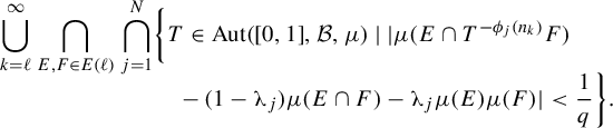
Our first claim is that $\mathcal O(\phi _1,\ldots ,\phi _N)=\bigcap _{q,\ell \in \mathbb {N}}\mathcal O(q,\ell )$
. Clearly, if
$\mathcal O(\phi _1,\ldots ,\phi _N)=\bigcap _{q,\ell \in \mathbb {N}}\mathcal O(q,\ell )$
. Clearly, if $T\in \mathcal O(\phi _1,\ldots , \phi _N)$
, then
$T\in \mathcal O(\phi _1,\ldots , \phi _N)$
, then $T\in \bigcap _{q,\ell \in \mathbb {N}}\mathcal O(q,\ell )$
. Now suppose that
$T\in \bigcap _{q,\ell \in \mathbb {N}}\mathcal O(q,\ell )$
. Now suppose that $T\in \bigcap _{q,\ell \in \mathbb {N}}\mathcal O(q,\ell )$
. It follows that, for each
$T\in \bigcap _{q,\ell \in \mathbb {N}}\mathcal O(q,\ell )$
. It follows that, for each $\ell \in \mathbb {N}$
, we can find a
$\ell \in \mathbb {N}$
, we can find a $k_\ell \geq \ell $
such that
$k_\ell \geq \ell $
such that
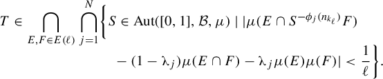
By passing to a subsequence, if needed, we can assume that $(k_\ell )_{\ell \in \mathbb {N}}$
is increasing. Furthermore, for any
$(k_\ell )_{\ell \in \mathbb {N}}$
is increasing. Furthermore, for any $m\in \mathbb {N}$
, any
$m\in \mathbb {N}$
, any $j\in \{1,\ldots ,N\}$
, and any
$j\in \{1,\ldots ,N\}$
, and any $E,F\in E(m)$
,
$E,F\in E(m)$
,
Note that for a fixed $F\in \mathcal B$
, the set
$F\in \mathcal B$
, the set $\mathcal E_F$
of those
$\mathcal E_F$
of those $E\in \mathcal B$
for which (5.2) holds is a
$E\in \mathcal B$
for which (5.2) holds is a $\unicode{x3bb} $
-system and that for a fixed
$\unicode{x3bb} $
-system and that for a fixed $E\in \mathcal B$
, the set
$E\in \mathcal B$
, the set $\Phi _E$
of those
$\Phi _E$
of those $F\in \mathcal B$
for which (5.2) holds is a
$F\in \mathcal B$
for which (5.2) holds is a $\unicode{x3bb} $
-system as well. (Let D be a family of subsets of a non-empty set X. D is a
$\unicode{x3bb} $
-system as well. (Let D be a family of subsets of a non-empty set X. D is a $\unicode{x3bb} $
-system if: (1)
$\unicode{x3bb} $
-system if: (1) $X\in D$
; (2) if
$X\in D$
; (2) if $A,B\in D$
and
$A,B\in D$
and $A\subseteq B$
, then
$A\subseteq B$
, then $B\setminus A\in D$
; and (3) for any collection of sets
$B\setminus A\in D$
; and (3) for any collection of sets $\{A_n\,|\,n\in \mathbb {N}\}\subseteq D$
with
$\{A_n\,|\,n\in \mathbb {N}\}\subseteq D$
with $A_1\subseteq A_2\subseteq \ldots $
, one has
$A_1\subseteq A_2\subseteq \ldots $
, one has $\bigcup _{n\in \mathbb {N}}A_n\in D$
.) Also note that
$\bigcup _{n\in \mathbb {N}}A_n\in D$
.) Also note that $\bigcup _{\ell \in \mathbb {N}}E_\ell \cup \{\emptyset \}$
is a
$\bigcup _{\ell \in \mathbb {N}}E_\ell \cup \{\emptyset \}$
is a $\pi $
-system with
$\pi $
-system with $\bigcup _{\ell \in \mathbb {N}}E_\ell \cup \{\emptyset \}\subseteq \mathcal E_F$
for each
$\bigcup _{\ell \in \mathbb {N}}E_\ell \cup \{\emptyset \}\subseteq \mathcal E_F$
for each $F\in \bigcup _{\ell \in \mathbb {N}}E_\ell $
. (Let P be a family of subsets of a non-empty set X. P is a
$F\in \bigcup _{\ell \in \mathbb {N}}E_\ell $
. (Let P be a family of subsets of a non-empty set X. P is a $\pi $
-system if P is non-empty and for any
$\pi $
-system if P is non-empty and for any $A,B\in P$
,
$A,B\in P$
, $A\cap B\in P$
.) By applying the
$A\cap B\in P$
.) By applying the $\pi $
–
$\pi $
– $\unicode{x3bb} $
theorem (see, for example, [Reference Durrett6, Theorem 2.1.6]) to each
$\unicode{x3bb} $
theorem (see, for example, [Reference Durrett6, Theorem 2.1.6]) to each $\mathcal E_F$
,
$\mathcal E_F$
, $F\in \bigcup _{\ell \in \mathbb {N}}E_\ell $
, we see that (5.2) holds for any
$F\in \bigcup _{\ell \in \mathbb {N}}E_\ell $
, we see that (5.2) holds for any $E\in \mathcal B$
and any
$E\in \mathcal B$
and any $F\in \bigcup _{\ell \in \mathbb {N}}E_\ell $
. Applying the
$F\in \bigcup _{\ell \in \mathbb {N}}E_\ell $
. Applying the $\pi $
–
$\pi $
– $\unicode{x3bb} $
theorem again but now to each
$\unicode{x3bb} $
theorem again but now to each $\Phi _E$
,
$\Phi _E$
, $E\in \mathcal B$
, we obtain that (5.2) holds for arbitrary
$E\in \mathcal B$
, we obtain that (5.2) holds for arbitrary $E,F\in \mathcal B$
and hence
$E,F\in \mathcal B$
and hence $T\in \mathcal O(\phi _1,\ldots ,\phi _N)$
.
$T\in \mathcal O(\phi _1,\ldots ,\phi _N)$
.
We now show that $\mathcal O(\phi _1,\ldots ,\phi _N)$
is
$\mathcal O(\phi _1,\ldots ,\phi _N)$
is $G_{\!\delta }$
. For any
$G_{\!\delta }$
. For any $E,F\in \bigcup _{\ell \in \mathbb {N}}E_\ell $
, define the map
$E,F\in \bigcup _{\ell \in \mathbb {N}}E_\ell $
, define the map
 $$ \begin{align*}I_{E,F}:\operatorname{Aut}([0,1],\mathcal B,\mu)\rightarrow [0,1]\end{align*} $$
by $I_{E,F}(T)=\mu (E\cap TF)$
.
$I_{E,F}(T)=\mu (E\cap TF)$
.
Note that for any given $E,F\in \bigcup _{\ell \in \mathbb {N}}E_\ell $
,
$E,F\in \bigcup _{\ell \in \mathbb {N}}E_\ell $
, $|I_{E,F}(T)-I_{E,F}(S)|\leq \mu (TF\triangle SF)$
and hence
$|I_{E,F}(T)-I_{E,F}(S)|\leq \mu (TF\triangle SF)$
and hence $I_{E,F}$
is continuous (with respect to the weak topology). Recall that
$I_{E,F}$
is continuous (with respect to the weak topology). Recall that $\operatorname {Aut}([0,1],\mathcal B,\mu )$
is a topological group and so, for any
$\operatorname {Aut}([0,1],\mathcal B,\mu )$
is a topological group and so, for any $n\in \mathbb {Z}$
, the map
$n\in \mathbb {Z}$
, the map $T\mapsto T^n$
is continuous. Thus, for each
$T\mapsto T^n$
is continuous. Thus, for each $n\in \mathbb {Z}$
and any
$n\in \mathbb {Z}$
and any $E,F\in \bigcup _{\ell \in \mathbb {N}}E_\ell $
, the map
$E,F\in \bigcup _{\ell \in \mathbb {N}}E_\ell $
, the map $T\mapsto \mu (E\cap T^nF)$
from
$T\mapsto \mu (E\cap T^nF)$
from $\operatorname {Aut}([0,1],\mathcal B,\mu )$
to
$\operatorname {Aut}([0,1],\mathcal B,\mu )$
to $[0,1]$
is continuous as well. It now follows that for any
$[0,1]$
is continuous as well. It now follows that for any $q,\ell \in \mathbb {N}$
,
$q,\ell \in \mathbb {N}$
, $\mathcal O(q,\ell )$
is open and hence
$\mathcal O(q,\ell )$
is open and hence $\mathcal O(\phi _1,\ldots ,\phi _N)$
is
$\mathcal O(\phi _1,\ldots ,\phi _N)$
is $G_{\!\delta }$
.
$G_{\!\delta }$
.
To prove that $\mathcal O(\phi _1,\ldots ,\phi _N)$
is dense, it suffices to show that for any
$\mathcal O(\phi _1,\ldots ,\phi _N)$
is dense, it suffices to show that for any $q,\ell \in \mathbb {N}$
, any
$q,\ell \in \mathbb {N}$
, any $T_0\in \operatorname {Aut}([0,1],\mathcal B,\mu )$
, and any
$T_0\in \operatorname {Aut}([0,1],\mathcal B,\mu )$
, and any $\epsilon>0$
, there exists a
$\epsilon>0$
, there exists a $T\in \mathcal O(q,\ell )$
such that
$T\in \mathcal O(q,\ell )$
such that $\partial (T_0,T)<\epsilon $
. In what follows, we will construct a transformation
$\partial (T_0,T)<\epsilon $
. In what follows, we will construct a transformation $T\in \operatorname {Aut}([0,1],\mathcal B,\mu )$
with these properties.
$T\in \operatorname {Aut}([0,1],\mathcal B,\mu )$
with these properties.
Fix $q,\ell \in \mathbb {N}$
,
$q,\ell \in \mathbb {N}$
, $T_0\in \operatorname {Aut}([0,1],\mathcal B,\mu )$
, and
$T_0\in \operatorname {Aut}([0,1],\mathcal B,\mu )$
, and $\epsilon>0$
. By Lemma 5.2, there exists a cyclic permutation R of the dyadic intervals of rank
$\epsilon>0$
. By Lemma 5.2, there exists a cyclic permutation R of the dyadic intervals of rank $\ell '$
for some
$\ell '$
for some $\ell '\geq \ell $
such that
$\ell '\geq \ell $
such that
 $$ \begin{align} \frac{1}{2^{\ell'}}<\frac{\epsilon}{4}\quad\text{and}\quad\partial (T_0,R)<\frac{\epsilon}{2}. \end{align} $$
By reindexing $\phi _1,\ldots ,\phi _N$
, if needed, we assume without loss of generality that
$\phi _1,\ldots ,\phi _N$
, if needed, we assume without loss of generality that
(we will actually assume that $0<\unicode{x3bb} _1<\cdots <\unicode{x3bb} _N<1$
, the general case is handled similarly).
$0<\unicode{x3bb} _1<\cdots <\unicode{x3bb} _N<1$
, the general case is handled similarly).
By assumption, there exist aperiodic $T_1,\ldots ,T_{N+1}\in \operatorname {Aut}([0,1],\mathcal B,\mu )$
such that for each
$T_1,\ldots ,T_{N+1}\in \operatorname {Aut}([0,1],\mathcal B,\mu )$
such that for each $t\in \{1,\ldots ,N+1\}$
, each
$t\in \{1,\ldots ,N+1\}$
, each $j\in \{1,\ldots ,N\}$
, and each
$j\in \{1,\ldots ,N\}$
, and each $A,B\in \mathcal B$
,
$A,B\in \mathcal B$
,
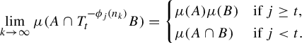 $$ \begin{align*}\lim_{k\rightarrow\infty}\mu(A\cap T_t^{- \phi_j(n_k)}B)=\begin{cases} \mu(A)\mu(B)&\text{if }j\geq t,\\ \mu(A\cap B)&\text{if }j<t. \end{cases}\end{align*} $$
By Lemma 5.3, we can assume that for each $t\in \{1,\ldots ,N+1\}$
,
$t\in \{1,\ldots ,N+1\}$
,
 $$ \begin{align} \partial (R,T_t)<\frac{\epsilon}{4}. \end{align} $$
Furthermore, since the set $\{T_t^n1\,|\,n\in \mathbb {Z}\}$
has measure zero, we assume without loss of generality that
$\{T_t^n1\,|\,n\in \mathbb {Z}\}$
has measure zero, we assume without loss of generality that $T_t(1)=1$
. Thus, for each
$T_t(1)=1$
. Thus, for each $t\in \{1,\ldots ,N+1\}$
,
$t\in \{1,\ldots ,N+1\}$
, $T_t([0,1))=[0,1)$
.
$T_t([0,1))=[0,1)$
.
Let $\unicode{x3bb} _0=0$
and
$\unicode{x3bb} _0=0$
and $\unicode{x3bb} _{N+1}=1$
. For each
$\unicode{x3bb} _{N+1}=1$
. For each $t\in \{1,\ldots ,N+1\}$
, let
$t\in \{1,\ldots ,N+1\}$
, let $\delta _t=\unicode{x3bb} _t-\unicode{x3bb} _{t-1}$
and let
$\delta _t=\unicode{x3bb} _t-\unicode{x3bb} _{t-1}$
and let
be defined by
for any $x\in [{r}/{2^{\ell '}},({r+1})/{2^{\ell '}})$
. We remark that
$x\in [{r}/{2^{\ell '}},({r+1})/{2^{\ell '}})$
. We remark that $S_t$
is a bijection and both
$S_t$
is a bijection and both $S_t$
and
$S_t$
and $S^{-1}_t$
are measurable.
$S^{-1}_t$
are measurable.
We now define $T:[0,1]\rightarrow [0,1]$
by
$T:[0,1]\rightarrow [0,1]$
by
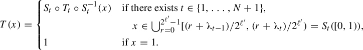
It now remains to show that: (i) $T\in \operatorname {Aut}([0,1],\mathcal B,\mu )$
; (ii)
$T\in \operatorname {Aut}([0,1],\mathcal B,\mu )$
; (ii) $T\in \mathcal O(q,\ell )$
; and (iii)
$T\in \mathcal O(q,\ell )$
; and (iii) $\partial (T_0,T)<\epsilon $
.
$\partial (T_0,T)<\epsilon $
.
(i) We will now show that $T\in \operatorname {Aut}([0,1],\mathcal B,\mu )$
. For each
$T\in \operatorname {Aut}([0,1],\mathcal B,\mu )$
. For each $t\in \{1,\ldots ,N+1\}$
,
$t\in \{1,\ldots ,N+1\}$
,

is an invertible measurable function with measurable inverse $S_t\circ T_t^{-1}\circ S_t^{-1}$
. Note that for any measurable
$S_t\circ T_t^{-1}\circ S_t^{-1}$
. Note that for any measurable $A\subseteq [0,1)$
,
$A\subseteq [0,1)$
, $\mu (S_t(A))=\delta _t\mu (A)$
and, consequently, for any measurable
$\mu (S_t(A))=\delta _t\mu (A)$
and, consequently, for any measurable $A\subseteq S_t([0,1))$
,
$A\subseteq S_t([0,1))$
, $\mu (S_t^{-1}A)=({1}/{\delta _t})\mu (A)$
. It follows that for any measurable
$\mu (S_t^{-1}A)=({1}/{\delta _t})\mu (A)$
. It follows that for any measurable $A\subseteq S_t([0,1))$
,
$A\subseteq S_t([0,1))$
,
 $$ \begin{align} \kern-6pt \mu(S_t\circ T_t\circ S_t^{-1}(A))=\delta_t\mu(T_t\circ S_t^{-1}(A)) =\delta_t\mu( S_t^{-1}(A))=\delta_t\cdot\frac{1}{\delta_t}\mu(A)=\mu(A) \end{align} $$
and similarly $\mu (S_t\circ T_t^{-1}\circ S_t^{-1}(A))=\mu (A)$
.
$\mu (S_t\circ T_t^{-1}\circ S_t^{-1}(A))=\mu (A)$
.
Let $A\subseteq [0,1]$
be measurable and for each
$A\subseteq [0,1]$
be measurable and for each $t\in \{1,\ldots ,N+1\}$
, let
$t\in \{1,\ldots ,N+1\}$
, let $A_t=A\cap S_t([0,1))$
. Since
$A_t=A\cap S_t([0,1))$
. Since $A=\bigcup _{t=1}^{N+1}A_t$
up to a set of measure zero and
$A=\bigcup _{t=1}^{N+1}A_t$
up to a set of measure zero and $A_1,\ldots ,A_{N+1}$
are disjoint, (5.6) implies
$A_1,\ldots ,A_{N+1}$
are disjoint, (5.6) implies
 $$ \begin{align*}\mu(TA){\kern-1.5pt}={\kern-1.5pt}\mu\bigg({\kern-1.5pt}\bigcup_{t=1}^{N+1}{\kern-1.5pt}TA_t{\kern-1.5pt}\bigg)={\kern-2.2pt}\sum_{t=1}^{N+1}{\kern-1.5pt}\mu(S_t\circ T_t\circ S_t^{-1}(A_t))={\kern-2.2pt}\sum_{t=1}^{N+1}{\kern-1.5pt}\mu(A_t)=\mu\bigg({\kern-1.5pt}\bigcup_{t=1}^{N+1}{\kern-1.5pt}A_t{\kern-1.5pt}\bigg)=\mu(A)\end{align*} $$
and $\mu (T^{-1}A)=\mu (A)$
. Thus,
$\mu (T^{-1}A)=\mu (A)$
. Thus, $T\in \operatorname {Aut}([0,1],\mathcal B,\mu )$
.
$T\in \operatorname {Aut}([0,1],\mathcal B,\mu )$
.
(ii) To prove that $T\in \mathcal O(q,\ell )$
, we will first note that for each
$T\in \mathcal O(q,\ell )$
, we will first note that for each $E\in E(\ell ')$
and each
$E\in E(\ell ')$
and each $t\in \{1,\ldots ,N+1\}$
,
$t\in \{1,\ldots ,N+1\}$
, $E\cap S_t([0,1))=S_t(E)$
. We also note that, by (5.5), for any
$E\cap S_t([0,1))=S_t(E)$
. We also note that, by (5.5), for any $t\in \{1,\ldots ,N+1\}$
,
$t\in \{1,\ldots ,N+1\}$
, $T(S_t([0,1)))=S_t([0,1))$
. Thus, for any
$T(S_t([0,1)))=S_t([0,1))$
. Thus, for any $j\in \{1,\ldots ,N\}$
and any
$j\in \{1,\ldots ,N\}$
and any $E,F\in E(\ell )\subseteq E(\ell ')$
,
$E,F\in E(\ell )\subseteq E(\ell ')$
,
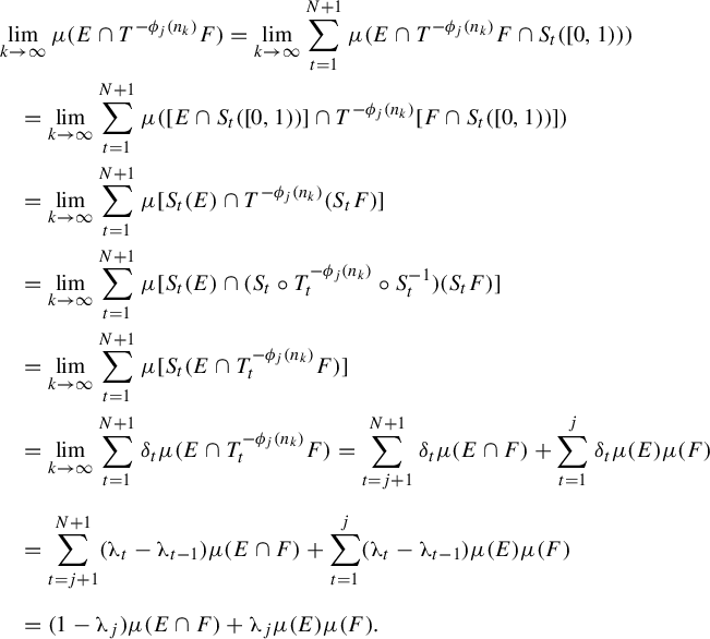
So $T\in \mathcal O(q,\ell )$
.
$T\in \mathcal O(q,\ell )$
.
(iii) By (5.3), to prove that $\partial (T_0,T)<\epsilon $
, all we need to show is that
$\partial (T_0,T)<\epsilon $
, all we need to show is that $\partial (R,T)<{\epsilon }/{2}$
. Note that for any
$\partial (R,T)<{\epsilon }/{2}$
. Note that for any $E\in E_{\ell '}$
,
$E\in E_{\ell '}$
, $RE\in E_{\ell '}$
. So, for any
$RE\in E_{\ell '}$
. So, for any $E\in E(\ell ')$
and any
$E\in E(\ell ')$
and any $t\in \{1,\ldots ,N+1\}$
,
$t\in \{1,\ldots ,N+1\}$
, $RE\cap S_t([0,1))=S_t(R(E))$
. It follows that
$RE\cap S_t([0,1))=S_t(R(E))$
. It follows that
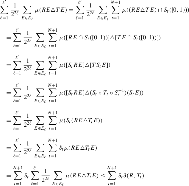 $$ \begin{align*} &\sum_{\ell=1}^{\ell'}\frac{1}{2^{2\ell}}\sum_{E\in E_\ell} \mu(RE\triangle TE)=\sum_{\ell=1}^{\ell'}\frac{1}{2^{2\ell}}\sum_{E\in E_\ell}\sum_{t=1}^{N+1} \mu((RE\triangle TE)\cap S_t([0,1)))\\[6pt]&\quad=\sum_{\ell=1}^{\ell'}\frac{1}{2^{2\ell}}\sum_{E\in E_\ell}\sum_{t=1}^{N+1} \mu([RE\cap S_t([0,1))]\triangle [TE\cap S_t([0,1))])\\[6pt]&\quad=\sum_{\ell=1}^{\ell'}\frac{1}{2^{2\ell}}\sum_{E\in E_\ell}\sum_{t=1}^{N+1} \mu([S_tRE]\triangle [TS_tE])\\[6pt]&\quad=\sum_{\ell=1}^{\ell'}\frac{1}{2^{2\ell}}\sum_{E\in E_\ell}\sum_{t=1}^{N+1} \mu([S_tRE]\triangle (S_t\circ T_t \circ S ^{-1}_t)(S_tE))\\[6pt]&\quad= \sum_{\ell=1}^{\ell'}\frac{1}{2^{2\ell}}\sum_{E\in E_\ell}\sum_{t=1}^{N+1} \mu(S_t(RE\triangle T_t E))\\[6pt]&\quad=\sum_{\ell=1}^{\ell'}\frac{1}{2^{2\ell}}\sum_{E\in E_\ell}\sum_{t=1}^{N+1}\delta_t\mu(RE\triangle T_tE)\\[6pt]&\quad=\sum_{t=1}^{N+1}\delta_t\sum_{\ell=1}^{\ell'}\frac{1}{2^{2\ell}}\sum_{E\in E_\ell}\mu(RE\triangle T_tE)\leq \sum_{t=1}^{N+1}\delta_t\partial(R,T_t). \end{align*} $$
By (5.4), $\partial (R,T_t)<{\epsilon }/{4}$
, so
$\partial (R,T_t)<{\epsilon }/{4}$
, so
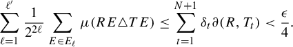 $$ \begin{align*} \sum_{\ell=1}^{\ell'}\frac{1}{2^{2\ell}}\sum_{E\in E_\ell} \mu(RE\triangle TE)\leq \sum_{t=1}^{N+1}\delta_t\partial(R,T_t)<\frac{\epsilon}{4}.\end{align*} $$
Finally, since by our choice of $\ell '$
,
$\ell '$
, ${1}/{2^{\ell '}}<{\epsilon }/{4}$
, we obtain
${1}/{2^{\ell '}}<{\epsilon }/{4}$
, we obtain
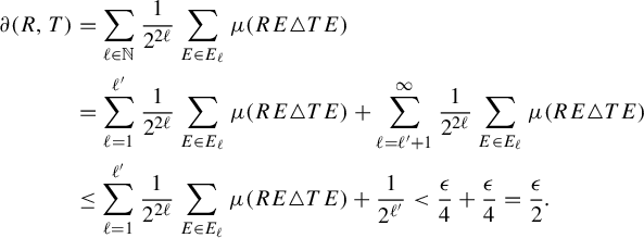 $$ \begin{align*} \partial (R,T)&=\sum_{\ell\in\mathbb{N}}\frac{1}{2^{2\ell}}\sum_{E\in E_\ell}\mu(RE\triangle TE)\\ &=\sum_{\ell=1}^{\ell'}\frac{1}{2^{2\ell}}\sum_{E\in E_\ell} \mu(RE\triangle TE)+\sum_{\ell=\ell'+1}^\infty \frac{1}{2^{2\ell}}\sum_{E\in E_\ell}\mu(RE\triangle TE)\\ &\leq\sum_{\ell=1}^{\ell'}\frac{1}{2^{2\ell}}\sum_{E\in E_\ell} \mu(RE\triangle TE)+\frac{1}{2^{\ell'}}<\frac{\epsilon}{4}+\frac{\epsilon}{4}=\frac{\epsilon}{2}. \end{align*} $$
We are done.
We now obtain Theorem 1.2 as a corollary of Theorems 4.2 and 5.1.
Theorem 5.4. Let $N\in \mathbb {N}$
and let
$N\in \mathbb {N}$
and let $\unicode{x3bb} _1,\ldots ,\unicode{x3bb} _N\in [0,1]$
. For any asymptotically independent sequences
$\unicode{x3bb} _1,\ldots ,\unicode{x3bb} _N\in [0,1]$
. For any asymptotically independent sequences $\phi _1,\ldots ,\phi _N:\mathbb {N}\rightarrow \mathbb {Z}$
, the set
$\phi _1,\ldots ,\phi _N:\mathbb {N}\rightarrow \mathbb {Z}$
, the set

is a dense $G_{\!\delta }$
set.
$G_{\!\delta }$
set.


6 Families of non-asymptotically independent sequences for which Condition C holds
In this section, we will show that, as mentioned in §1, Condition C in Theorem 1.3 is satisfied by families of sequences which are not asymptotically independent. The following result, which also follows from [Reference Bergelson, Kasjan and Lemańczyk3, Theorem 3.11], provides some examples of such families of sequences. (Our proof is different from that of [Reference Bergelson, Kasjan and Lemańczyk3, Theorem 3.11].)
Theorem 6.1. Let $N\geq 2$
, let
$N\geq 2$
, let $A_1,\ldots ,A_{2^N-2}$
be an enumeration of the non-empty proper subsets of
$A_1,\ldots ,A_{2^N-2}$
be an enumeration of the non-empty proper subsets of $\{1,\ldots ,N\}$
, and let
$\{1,\ldots ,N\}$
, and let $p_1,\ldots ,p_{2^N-2}\in \mathbb {N}$
be distinct prime numbers. For each
$p_1,\ldots ,p_{2^N-2}\in \mathbb {N}$
be distinct prime numbers. For each $j\in \{1,\ldots ,N\}$
, set
$j\in \{1,\ldots ,N\}$
, set
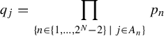 $$ \begin{align} q_j=\prod_{\{n\in\{1,\ldots,2^N-2\}\,|\,j\in A_n\}}p_n \end{align} $$
and put $\phi _j(k)=q_jk$
,
$\phi _j(k)=q_jk$
, $k\in \mathbb {N}$
. Then there exists an increasing sequence
$k\in \mathbb {N}$
. Then there exists an increasing sequence $(n_k)_{k\in \mathbb {N}}$
in
$(n_k)_{k\in \mathbb {N}}$
in $\mathbb {N}$
such that for any
$\mathbb {N}$
such that for any $\vec \xi =(\xi _1,\ldots ,\xi _N)\in \{0,1\}^N$
, there exists a non-trivial weakly mixing Gaussian system
$\vec \xi =(\xi _1,\ldots ,\xi _N)\in \{0,1\}^N$
, there exists a non-trivial weakly mixing Gaussian system $(\mathbb {R}^{\mathbb {Z}},\mathcal A,\gamma _{\vec \xi },T_{\vec \xi })$
with the property that for each
$(\mathbb {R}^{\mathbb {Z}},\mathcal A,\gamma _{\vec \xi },T_{\vec \xi })$
with the property that for each $j\in \{1,\ldots ,N\}$
and any
$j\in \{1,\ldots ,N\}$
and any $A,B\in \mathcal A$
,
$A,B\in \mathcal A$
,
 $$ \begin{align} \lim_{k\rightarrow\infty}\gamma_{\kern1.5pt\vec\xi}(A\cap T_{\vec \xi}^{- \phi_j(n_k) }B)=(1-\xi_j)\gamma_{\kern1.5pt\vec\xi}(A\cap B)+\xi_j\gamma_{\kern1.5pt\vec\xi}(A)\gamma_{\kern1.5pt\vec\xi}(B). \end{align} $$
Proof. Let $A_0=\{1,\ldots ,N\}$
, let
$A_0=\{1,\ldots ,N\}$
, let $A_{2^N-1}=\emptyset $
, and let M be the least prime number with the property that for each
$A_{2^N-1}=\emptyset $
, and let M be the least prime number with the property that for each $n\in \{1,\ldots ,2^N-2\}$
,
$n\in \{1,\ldots ,2^N-2\}$
, $M>p_n$
. Put
$M>p_n$
. Put $p_{2^N-1}=M$
and define the sequence
$p_{2^N-1}=M$
and define the sequence $(n_k)_{k\in \mathbb {N}}$
by
$(n_k)_{k\in \mathbb {N}}$
by
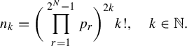 $$ \begin{align*}n_k=\bigg(\prod_{r=1}^{2^N-1}p_r\bigg)^{2k}k!\!,\quad k\in\mathbb{N}.\end{align*} $$
For each $n\in \{0,\ldots ,2^N-1\}$
, define
$n\in \{0,\ldots ,2^N-1\}$
, define $\vec \xi _n=(\xi _1^{(n)},\ldots ,\xi _N^{(n)})\in \{0,1\}^N$
by
$\vec \xi _n=(\xi _1^{(n)},\ldots ,\xi _N^{(n)})\in \{0,1\}^N$
by
(Observe that $\{\vec \xi _n\,|\,n\in \{0,\ldots ,2^N-1\}\}=\{0,1\}^N$
.)
$\{\vec \xi _n\,|\,n\in \{0,\ldots ,2^N-1\}\}=\{0,1\}^N$
.)
Fix $n\in \{0,1,\ldots ,2^N-1\}$
, put
$n\in \{0,1,\ldots ,2^N-1\}$
, put $p_0=1$
, and let
$p_0=1$
, and let $c_n=\max \{p_n-1,1\}$
. Consider the product space
$c_n=\max \{p_n-1,1\}$
. Consider the product space
 $$ \begin{align*}X_n=\{0,\ldots,c_n\}^{\mathbb{N}}\end{align*} $$
and let $\mathbb P_n$
be the Borel probability measure on
$\mathbb P_n$
be the Borel probability measure on $X_n$
defined by the infinite product of the normalized counting measure on
$X_n$
defined by the infinite product of the normalized counting measure on $\{0,\ldots ,c_n\}$
. Let
$\{0,\ldots ,c_n\}$
. Let $f_n:X_n\times X_n\rightarrow \mathbb T$
be defined by
$f_n:X_n\times X_n\rightarrow \mathbb T$
be defined by
 $$ \begin{align*}f_n(\omega_1,\omega_2)=\sum_{t=1}^\infty\frac{1}{n_t}\frac{\omega_1(t)-\omega_2(t)}{p_n}\ \textrm{mod}\,1.\end{align*} $$
Clearly, $f_n$
is continuous.
$f_n$
is continuous.
Set the probability measure $\sigma _{\vec \xi _n}$
on
$\sigma _{\vec \xi _n}$
on $\mathbb T$
to equal
$\mathbb T$
to equal
![]() . Note that for each
. Note that for each $k\in \mathbb {Z}$
,
$k\in \mathbb {Z}$
,
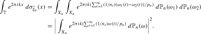 $$ \begin{align*} \int_{\mathbb T} e^{2\pi ikx}\,d\sigma_{\vec \xi_n}(x)&=\int_{X_n}\int_{X_n}e^{2\pi i k(\sum_{t=1}^\infty({1}/{n_t})({\omega_1(t)-\omega_2(t)})/{p_n})}\,d\mathbb P_n(\omega_1)\,d\mathbb P_n(\omega_2)\\ &=\bigg|\int_{X_n}e^{2\pi ik(\sum_{t=1}^\infty({1}/{n_t}){\omega(t)}/{p_n})}\,d\mathbb P_n(\omega)\bigg|^2. \end{align*} $$
It follows that $\sigma _{\vec \xi _n}$
is a (non-zero, positive) symmetric probability measure. We claim that the non-trivial Gaussian system
$\sigma _{\vec \xi _n}$
is a (non-zero, positive) symmetric probability measure. We claim that the non-trivial Gaussian system $(\mathbb {R}^{\mathbb {Z}},\mathcal A,\gamma _{\vec \xi _n}, T_{\vec \xi _n})$
associated with
$(\mathbb {R}^{\mathbb {Z}},\mathcal A,\gamma _{\vec \xi _n}, T_{\vec \xi _n})$
associated with $\sigma _{\vec \xi _n}$
is weakly mixing and satisfies (6.2). By Proposition 2.4 and Theorem 2.3, it suffices to show that: (i)
$\sigma _{\vec \xi _n}$
is weakly mixing and satisfies (6.2). By Proposition 2.4 and Theorem 2.3, it suffices to show that: (i) $\sigma _{\vec \xi _n}$
is continuous and (ii) that for each
$\sigma _{\vec \xi _n}$
is continuous and (ii) that for each $j\in \{1,\ldots ,N\}$
and any
$j\in \{1,\ldots ,N\}$
and any $m\in \mathbb {Z}$
,
$m\in \mathbb {Z}$
,
 $$ \begin{align} \lim_{k\rightarrow\infty}\int_{\mathbb T} e^{2\pi i(\phi_j(n_k)+m)x}\,d\sigma_{\vec\xi_n}(x)=(1-\xi_j^{(n)})\int_{\mathbb T} e^{2\pi imx}\,d\sigma_{\vec\xi_n}(x). \end{align} $$
(i) We will now show that $\sigma _{\vec \xi _n}$
is continuous. For this, let
$\sigma _{\vec \xi _n}$
is continuous. For this, let $j\in \{1,\ldots ,N\}$
and note that
$j\in \{1,\ldots ,N\}$
and note that
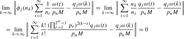 $$ \begin{align} &\lim_{k\rightarrow\infty}\bigg\|\phi_j(n_k)\sum_{t=1}^\infty\frac{1}{n_t}\frac{\omega(t)}{p_nM}-\frac{q_j\omega(k)}{p_nM}\bigg\|=\lim_{k\rightarrow\infty}\bigg\|\sum_{t=1}^\infty\frac{n_k}{n_t}\frac{q_j\omega(t)}{p_nM}-\frac{q_j\omega(k)}{p_nM}\bigg\|\nonumber\\ &\quad=\lim_{k\rightarrow\infty}\bigg\|\sum_{t=1}^\infty\frac{k!}{t!}\frac{(\prod_{r=1}^{2^N-1}p_r)^{2(k-t)}q_j\omega(t)}{p_nM}-\frac{q_j\omega(k)}{p_nM}\bigg\|=0 \end{align} $$
uniformly in $\omega \in X_n$
. Thus,
$\omega \in X_n$
. Thus,
 $$ \begin{align} \lim_{k\rightarrow\infty}\bigg\|\phi_j(n_k)\sum_{t=1}^\infty\frac{1}{n_t}\frac{\omega_1(t)}{p_nM}-\phi_j(n_k)\sum_{t=1}^\infty\frac{1}{n_t}\frac{\omega_2(t)}{p_nM}\bigg\|-\bigg\|\frac{q_j\omega_1(k)}{p_nM}-\frac{q_j\omega_2(k)}{p_nM}\bigg\|=0 \end{align} $$
uniformly in $(\omega _1,\omega _2)\in X_n\times X_n$
.
$(\omega _1,\omega _2)\in X_n\times X_n$
.
By (6.1), $q_j$
and M are relatively prime and hence for any
$q_j$
and M are relatively prime and hence for any $a,b\in \{0,\ldots ,c_n\}$
,
$a,b\in \{0,\ldots ,c_n\}$
,
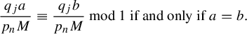 $$ \begin{align} \frac{q_ja}{p_nM}\equiv\frac{q_jb}{p_nM}\,\text{mod}\,1\text{ if and only if}\ a=b. \end{align} $$
The continuity of $\sigma _{\vec \xi _n}$
now follows from (6.5) and (6.6) by noting that
$\sigma _{\vec \xi _n}$
now follows from (6.5) and (6.6) by noting that $\mathbb P_n$
is an atomless measure and arguing as in the proof of Theorem 3.1.
$\mathbb P_n$
is an atomless measure and arguing as in the proof of Theorem 3.1.
(ii) By (6.4), for any $j\in \{1,\ldots ,N\}$
,
$j\in \{1,\ldots ,N\}$
,
 $$ \begin{align*} \lim_{k\rightarrow\infty}{\kern-1.5pt}\bigg\|\phi_j(n_k){\kern-1.5pt}\sum_{t=1}^\infty\frac{1}{n_t}\frac{\omega(t)}{p_n}-\frac{q_j\omega(k)}{p_n}\bigg\|{\kern-1.5pt} = \lim_{k\rightarrow\infty}|M|\bigg\|\phi_j(n_k){\kern-1.5pt}\sum_{t=1}^\infty\frac{1}{n_t}\frac{\omega(t)}{p_nM}-\frac{q_j(\omega(k)}{p_nM}\bigg\|{\kern-1.5pt}=0 \end{align*} $$
uniformly on $\omega \in X_n$
. So for each
$\omega \in X_n$
. So for each $m\in \mathbb {Z}$
,
$m\in \mathbb {Z}$
,
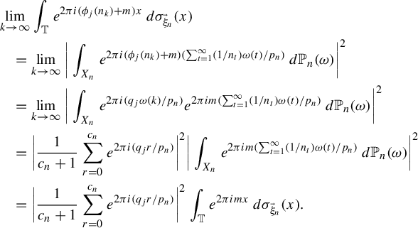 $$ \begin{align*} &\lim_{k\rightarrow\infty}\int_{\mathbb T} e^{2\pi i (\phi_j(n_k)+m)x}\,d\sigma_{\vec \xi_n}(x)\\ &\quad=\lim_{k\rightarrow\infty} \bigg|\int_{X_n}e^{2\pi i(\phi_j(n_k)+m)(\sum_{t=1}^\infty({1}/{n_t}){\omega(t)}/{p_n})}\,d\mathbb P_n(\omega)\bigg|^2\\ &\quad=\lim_{k\rightarrow\infty} \bigg|\int_{X_n}e^{2\pi i({q_j\omega(k)}/{p_n})}e^{2\pi i m(\sum_{t=1}^\infty({1}/{n_t}){\omega(t)}/{p_n})}\,d\mathbb P_n(\omega)\bigg|^2\\ &\quad=\bigg|\frac{1}{c_n+1}\sum_{r=0}^{c_n}e^{2\pi i({q_jr}/{p_n})}\bigg|^2\bigg|\int_{X_n}e^{2\pi i m(\sum_{t=1}^\infty({1}/{n_t}){\omega(t)}/{p_n})}\,d\mathbb P_n(\omega)\bigg|^2\\ &\quad=\bigg|\frac{1}{c_n+1}\sum_{r=0}^{c_n}e^{2\pi i({q_jr}/{p_n})}\bigg|^2\int_{\mathbb T} e^{2\pi imx}\,d\sigma_{\vec \xi_n}(x). \end{align*} $$
By (6.1), for each $j\in \{1,\ldots ,N\}$
,
$j\in \{1,\ldots ,N\}$
,
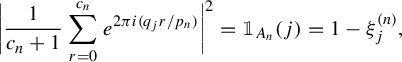
which implies that (6.3) holds.
Acknowledgments
The author would like to thank Professor Vitaly Bergelson for the question which motivated this paper and his valuable input during the preparation of the manuscript. The author also thanks the referee to whom the much clearer and more succinct presentation of the material in §2 is owed.

 Open access