


1 Introduction
The present paper is a continuation of [Reference Mukhamedov and Khakimov35], where we have started to investigate the chaotic behavior of the Potts–Bethe mapping over the p-adic field (here p is some prime number). Note that the mapping is governed by
 $$ \begin{align} f_{\theta,q,k}(x)=\bigg(\frac{\theta x+q-1}{x+\theta+q-2}\bigg)^k, \end{align} $$
where $k,q\in \mathbb N$
and
$k,q\in \mathbb N$
and $|\theta -1|_p<1$
. In [Reference Mukhamedov and Khakimov35], we have considered the case when q is not divisible by p, that is,
$|\theta -1|_p<1$
. In [Reference Mukhamedov and Khakimov35], we have considered the case when q is not divisible by p, that is, $|q|_p=1$
. In that setting, under some conditions, we were able to prove that
$|q|_p=1$
. In that setting, under some conditions, we were able to prove that $f_{\theta ,q,k}$
is conjugate to the full shift on
$f_{\theta ,q,k}$
is conjugate to the full shift on $\kappa _p$
symbols (here
$\kappa _p$
symbols (here $\kappa _p$
is the greatest common factor (GCF) of k and
$\kappa _p$
is the greatest common factor (GCF) of k and $p-1$
). In the current paper, we are going to study the same Potts–Bethe mapping when q is divisible by p, that is
$p-1$
). In the current paper, we are going to study the same Potts–Bethe mapping when q is divisible by p, that is $|q|_p<1$
. It is known that the thermodynamic behavior of the central site of the Potts model with nearest-neighbor interactions on a Cayley tree is reduced to the recursive system which is given by (1.1). The existence of at least two non-trivial p-adic Gibbs measures indicates that the phase transition may exist. This is closely connected to the chaotic behavior of the associated dynamical system [Reference Fan and Liao12, Reference Khakimov16, Reference Khakimov17, Reference Monroe23, Reference Mukhamedov26, Reference Mukhamedov27]. Therefore, it is important to investigate the chaotic properties of (1.1).
$|q|_p<1$
. It is known that the thermodynamic behavior of the central site of the Potts model with nearest-neighbor interactions on a Cayley tree is reduced to the recursive system which is given by (1.1). The existence of at least two non-trivial p-adic Gibbs measures indicates that the phase transition may exist. This is closely connected to the chaotic behavior of the associated dynamical system [Reference Fan and Liao12, Reference Khakimov16, Reference Khakimov17, Reference Monroe23, Reference Mukhamedov26, Reference Mukhamedov27]. Therefore, it is important to investigate the chaotic properties of (1.1).
We stress that the Potts–Ising mapping is a particular case of the Potts–Bethe mapping, which can be obtained from (1.1) by putting $q=2$
. Recently, in [Reference Mukhamedov, Akin and Dogan30, Reference Mukhamedov and Khakimov34] under some condition, a Julia set of the Potts–Ising mapping was described, and it was shown that restricted to its Julia set, the Potts–Ising mapping is conjugate to a full shift. Therefore, it is natural to consider the Potts–Bethe mapping for
$q=2$
. Recently, in [Reference Mukhamedov, Akin and Dogan30, Reference Mukhamedov and Khakimov34] under some condition, a Julia set of the Potts–Ising mapping was described, and it was shown that restricted to its Julia set, the Potts–Ising mapping is conjugate to a full shift. Therefore, it is natural to consider the Potts–Bethe mapping for $q\geq 3$
with
$q\geq 3$
with $|q|_p<1$
and
$|q|_p<1$
and $k\geq 2$
. In [Reference Rozikov and Khakimov43], all fixed points of
$k\geq 2$
. In [Reference Rozikov and Khakimov43], all fixed points of $f_{\theta ,q,k}$
were found when
$f_{\theta ,q,k}$
were found when $k=2$
and
$k=2$
and $|q|_p<1$
. Then, using these fixed points, the dynamics of (1.1) whenever
$|q|_p<1$
. Then, using these fixed points, the dynamics of (1.1) whenever $k=2$
and
$k=2$
and $|q|_p<1$
was investigated in [Reference Fan, Fan, Liao and Wang11, Reference Mukhamedov and Khakimov31, Reference Mukhamedov and Khakimov32]. Recently in [Reference Ahmad, Liao and Saburov1, Reference Saburov and Ahmad44], the Potts–Bethe mapping was studied for the case
$|q|_p<1$
was investigated in [Reference Fan, Fan, Liao and Wang11, Reference Mukhamedov and Khakimov31, Reference Mukhamedov and Khakimov32]. Recently in [Reference Ahmad, Liao and Saburov1, Reference Saburov and Ahmad44], the Potts–Bethe mapping was studied for the case $k=3$
and
$k=3$
and $|q|_p<1$
. In the present paper, we are going to consider a more general case, that is, arbitrary
$|q|_p<1$
. In the present paper, we are going to consider a more general case, that is, arbitrary $k\geq 2$
and
$k\geq 2$
and $|q|_p<1$
. To formulate our main result, let us recall some necessary notions.
$|q|_p<1$
. To formulate our main result, let us recall some necessary notions.
It is easy to notice that the function (1.1) is defined on $\mathbb Q_p\setminus \{x^{(\infty )}\}$
, where
$\mathbb Q_p\setminus \{x^{(\infty )}\}$
, where $x^{(\infty )}=2-q-\theta $
. For the sake of convenience, we write
$x^{(\infty )}=2-q-\theta $
. For the sake of convenience, we write $\text {Dom}(f_{\theta ,q,k}):=\mathbb Q_p\setminus \{x^{(\infty )}\}$
. Let us denote
$\text {Dom}(f_{\theta ,q,k}):=\mathbb Q_p\setminus \{x^{(\infty )}\}$
. Let us denote
 $$ \begin{align*}\mathcal P_{x^{(\infty)}}=\bigcup_{n=1}^\infty f_{\theta,q,k}^{-n}(x^{(\infty)}). \end{align*} $$
One can see that the set $\mathcal P_{x^{(\infty )}}$
is at most countable, and could be empty for some
$\mathcal P_{x^{(\infty )}}$
is at most countable, and could be empty for some $k,q$
and
$k,q$
and $\theta $
(see §3). If it is not empty, then for any
$\theta $
(see §3). If it is not empty, then for any $x_0\in \mathcal P_{x^{(\infty )}}$
, there exists an
$x_0\in \mathcal P_{x^{(\infty )}}$
, there exists an $n\geq 1$
such that after n-times, we will ‘lose’ that point.
$n\geq 1$
such that after n-times, we will ‘lose’ that point.
For a given mapping f on $\mathbb Q_p$
, we denote by
$\mathbb Q_p$
, we denote by $\text {Fix}(f)$
the set of all fixed points of f, that is,
$\text {Fix}(f)$
the set of all fixed points of f, that is,
 $$ \begin{align*}\text{Fix}(f)=\{x\in\mathbb Q_p: f(x)=x\}. \end{align*} $$
Let f be an analytic function and $x^{(0)}\in \text {Fix}(f)$
. We define
$x^{(0)}\in \text {Fix}(f)$
. We define
 $$ \begin{align*}\lambda=\frac{d}{d x}f(x^{(0)}). \end{align*} $$
The fixed point $x^{(0)}$
is called attractive if
$x^{(0)}$
is called attractive if $0<|\lambda |_p<1$
, indifferent if
$0<|\lambda |_p<1$
, indifferent if $|\lambda |_p=1$
, and repelling if
$|\lambda |_p=1$
, and repelling if $|\lambda |_p>1$
.
$|\lambda |_p>1$
.
For an attractive fixed point $x^{(0)}$
of f, its basin of attraction is defined by
$x^{(0)}$
of f, its basin of attraction is defined by
 $$ \begin{align*}A(x^{(0)})=\{x\in\mathbb Q_p: \lim_{n\to\infty}f^n(x)=x^{(0)}\}, \end{align*} $$
where $f^n=\underbrace {f\circ f\circ \cdots \circ f}_n$
.
$f^n=\underbrace {f\circ f\circ \cdots \circ f}_n$
.
The main result of the present paper is given in the following theorem.
Theorem 1.1. Let $p\geq 3$
,
$p\geq 3$
, $k\geq 2$
,
$k\geq 2$
, $|q|_p<1$
,
$|q|_p<1$
, $|\theta -1|_p<1$
, and
$|\theta -1|_p<1$
, and $x_0^*=1$
. Then the dynamical structure of the system
$x_0^*=1$
. Then the dynamical structure of the system $(\mathbb Q_p, f_{\theta ,q,k})$
is described as follows.
$(\mathbb Q_p, f_{\theta ,q,k})$
is described as follows.
-
(A) If $|k|_p\leq |q+\theta -1|_p$
, then
$\mathrm{Fix}(f_{\theta ,q,k})=\{x_0^*\}$
and
$$ \begin{align*}A(x_0^*)=\mathrm{Dom}(f_{\theta,q,k}). \end{align*} $$
$|k|_p\leq |q+\theta -1|_p$
, then
$\mathrm{Fix}(f_{\theta ,q,k})=\{x_0^*\}$
and
$$ \begin{align*}A(x_0^*)=\mathrm{Dom}(f_{\theta,q,k}). \end{align*} $$
-
(B) Assume that
$|k|_p>|q+\theta -1|_p$
and
$|\theta -1|_p<|q|_p^2$
. Then there exists a non-empty set
$J_{f_{\theta ,q,k}}\subset \mathrm{Dom}(f_{\theta ,q,k})\setminus \mathcal P_{x^{(\infty )}}$
which is invariant with respect to
$f_{\theta ,q,k}$
and Moreover, if
$$ \begin{align*}A(x_0^*)=\mathrm{Dom}(f_{\theta,q,k})\setminus(\mathcal P_{x^{(\infty)}}\cup J_{f_{\theta,q,k}}). \end{align*} $$
$\kappa _p$
is the GCF of k and
$p-1$
, then the following hold:
-
(B1) if
$\kappa _p=1$
, then there exists
$x_*\in \mathrm{Fix}(f_{\theta ,q,k})$
such that
$x_*\neq x_0^*$
and
$J_{f_{\theta ,q,k}}=\{x_*\}$
; -
(B2) if
$\kappa _p\geq 2$
, then
$(J_{f_{\theta ,q,k}},f_{\theta ,q,k},|\cdot |_p)$
is topologically conjugate to the full shift dynamics on
$\kappa _p$
symbols.
-


Remark 1.2. It is worth pointing out that, in the present paper, the condition $|\theta -1|_p<|q|_p^2$
is assumed to get essential estimations and calculations to prove the main result. The results of a recent paper [Reference Ahmad, Liao and Saburov1] show that such a condition could be loosened to
$|\theta -1|_p<|q|_p^2$
is assumed to get essential estimations and calculations to prove the main result. The results of a recent paper [Reference Ahmad, Liao and Saburov1] show that such a condition could be loosened to $|\theta -1|_p<|q|_p$
, but only for the case
$|\theta -1|_p<|q|_p$
, but only for the case $k=3$
where explicit expressions of the fixed points of the function
$k=3$
where explicit expressions of the fixed points of the function $f_{\theta ,q,k}$
have essentially been used to get more exact estimations. However, in this paper, we are able to prove the chaoticity of the Potts–Bethe mapping for arbitrary values of k (under the condition
$f_{\theta ,q,k}$
have essentially been used to get more exact estimations. However, in this paper, we are able to prove the chaoticity of the Potts–Bethe mapping for arbitrary values of k (under the condition $|\theta -1|_p<|q|_p^2$
) and moreover, we are not even using the existence of the fixed points. Once we have proved that the Potts–Bethe mapping is conjugate to a full shift, then one concludes the existence of the fixed points. Roughly speaking, we are constructing (explicitly) a Markov partition of the mapping (1.1) which allows us to prove the main result of the current paper. However, the results of [Reference Ahmad, Liao and Saburov1] indicate that the chaoticity of the function (1.1) could be obtained even in the case of
$|\theta -1|_p<|q|_p^2$
) and moreover, we are not even using the existence of the fixed points. Once we have proved that the Potts–Bethe mapping is conjugate to a full shift, then one concludes the existence of the fixed points. Roughly speaking, we are constructing (explicitly) a Markov partition of the mapping (1.1) which allows us to prove the main result of the current paper. However, the results of [Reference Ahmad, Liao and Saburov1] indicate that the chaoticity of the function (1.1) could be obtained even in the case of $|q|^2\leq |\theta -1|_p<|q|_p$
, but this will be a topic for another work. Here, it is better to emphasize that the results are valid when
$|q|^2\leq |\theta -1|_p<|q|_p$
, but this will be a topic for another work. Here, it is better to emphasize that the results are valid when $p\geq 3$
. The case
$p\geq 3$
. The case $p=2$
is considered pathological in the p-adic analysis (see for example [Reference Fan, Liao, Wang and Zhou10]). Indeed, in [Reference Ahmad, Liao and Saburov1], it was established that when
$p=2$
is considered pathological in the p-adic analysis (see for example [Reference Fan, Liao, Wang and Zhou10]). Indeed, in [Reference Ahmad, Liao and Saburov1], it was established that when $p=2$
and
$p=2$
and $k=3$
, the function (1.1) does not have chaotic behavior. For general values of k, owing to huge calculations and numerous technical issues, this case could be investigated elsewhere.
$k=3$
, the function (1.1) does not have chaotic behavior. For general values of k, owing to huge calculations and numerous technical issues, this case could be investigated elsewhere.
Remark 1.3. In [Reference Mukhamedov and Rozikov41, Reference Mukhamedov and Rozikov42], the authors established that the function (1.1) may have at least one fixed point and, moreover, they found a necessary condition (that is q is divisible by p) for the existence of more than one fixed point. Therefore, the following conjecture was formulated: Let $k\in {\mathbb N}$
,
$k\in {\mathbb N}$
, $q\in p{\mathbb N}$
, and
$q\in p{\mathbb N}$
, and $|\theta -1|_p<1$
, then the function (1.1) has at least two fixed points. The formulated Theorem 1.1(A) shows that the mentioned conjecture is not always true.
$|\theta -1|_p<1$
, then the function (1.1) has at least two fixed points. The formulated Theorem 1.1(A) shows that the mentioned conjecture is not always true.
We stress that, in the p-adic setting, owing to the lack of a convex structure of the set of p-adic Gibbs measures, it was quite difficult to constitute a phase transition with some features of the set of p-adic Gibbs measures. However, Theorem 1.1(B2) yields that the set of p-adic Gibbs measures is huge which is a priori not clear (see [Reference Mukhamedov24, Reference Mukhamedov and Rozikov42]). Moreover, the method of the present work allows one to find lots of periodic p-adic Gibbs measures for the p-adic Potts model. Furthermore, Theorem 1.1(B) together with the results of [Reference Mukhamedov and Akin29, Reference Mukhamedov and Khakimov33] will open new perspectives in investigations of generalized p-adic self-similar sets.
On one hand, our results shed some light on the question of the investigation of dynamics of rational functions in the p-adic analysis, because a global dynamical structure of rational maps on $\mathbb {Q}_p$
remains unclear. Some particular rational functions have been considered in [Reference Benedetto4, Reference Benedetto5, Reference Diao and Silva7, Reference Ganikhodjaev, Mukhamedov and Rozikov8, Reference Fan, Liao, Wang and Zhou10, Reference Khakimov13–Reference Khakimov15, Reference Khamraev and Mukhamedov18, Reference Khrennikov and Nilsson21, Reference Mukhamedov, Saburov and Khakimov39]. On the other hand, the obtained results may have potential applications in the cryptography to build pseudo-random codes (see [Reference Anashin2, Reference Anashin, Khrennikov and Yurova3, Reference Mukhamedov, Omirov and Saburov37, Reference Woodcock and Smart45]). We point out that some p-adic chaotic dynamical systems have been studied in [Reference Gyorgyi, Kondor, Sasvari and Tel9, Reference Woodcock and Smart45].
$\mathbb {Q}_p$
remains unclear. Some particular rational functions have been considered in [Reference Benedetto4, Reference Benedetto5, Reference Diao and Silva7, Reference Ganikhodjaev, Mukhamedov and Rozikov8, Reference Fan, Liao, Wang and Zhou10, Reference Khakimov13–Reference Khakimov15, Reference Khamraev and Mukhamedov18, Reference Khrennikov and Nilsson21, Reference Mukhamedov, Saburov and Khakimov39]. On the other hand, the obtained results may have potential applications in the cryptography to build pseudo-random codes (see [Reference Anashin2, Reference Anashin, Khrennikov and Yurova3, Reference Mukhamedov, Omirov and Saburov37, Reference Woodcock and Smart45]). We point out that some p-adic chaotic dynamical systems have been studied in [Reference Gyorgyi, Kondor, Sasvari and Tel9, Reference Woodcock and Smart45].
2 Preliminaries
2.1 p-adic numbers
Let $\mathbb {Q}$
be the field of rational numbers. For a fixed prime number p, every rational number
$\mathbb {Q}$
be the field of rational numbers. For a fixed prime number p, every rational number $x\ne 0$
can be represented in the form
$x\ne 0$
can be represented in the form $x = p^r{n\over m}$
, where
$x = p^r{n\over m}$
, where $r, n\in \mathbb {Z}$
, m is a positive integer, and n and m are relatively prime with p:
$r, n\in \mathbb {Z}$
, m is a positive integer, and n and m are relatively prime with p: $(p, n) = 1$
,
$(p, n) = 1$
, $(p, m) = 1$
. The p-adic norm of x is given by
$(p, m) = 1$
. The p-adic norm of x is given by
 $$ \begin{align*}|x|_p=\left\{\begin{array}{@{}ll} p^{-r} \quad& \text{for } x\ne 0,\\ 0 \quad& \text{for } x = 0. \end{array}\right. \end{align*} $$
This norm is non-Archimedean and satisfies the so-called strong triangle inequality
 $$ \begin{align*}|x+y|_p\leq \max\{|x|_p,|y|_p\}.\end{align*} $$
The completion of $\mathbb {Q}$
with respect to the p-adic norm defines the p-adic field
$\mathbb {Q}$
with respect to the p-adic norm defines the p-adic field $\mathbb {Q}_p$
. Any p-adic number
$\mathbb {Q}_p$
. Any p-adic number $x\ne 0$
can be uniquely represented in the canonical form
$x\ne 0$
can be uniquely represented in the canonical form
 $$ \begin{align} x = p^{\mathrm{ord}_p(x)}(x_0+x_1p+x_2p^2+\cdots), \end{align} $$
where $\mathrm{ord}_p(x)\in \mathbb Z$
and the integers
$\mathrm{ord}_p(x)\in \mathbb Z$
and the integers $x_j$
satisfy:
$x_j$
satisfy: $0\leq x_j \leq p - 1$
,
$0\leq x_j \leq p - 1$
, $x_0\neq 0$
. In this case,
$x_0\neq 0$
. In this case, $|x|_p = p^{-\mathrm{ord}_p{x}}$
.
$|x|_p = p^{-\mathrm{ord}_p{x}}$
.
Recall that $\mathbb Q_p$
is not an ordered field. So, we may compare two p-adic numbers only with respect to their p-adic norms.
$\mathbb Q_p$
is not an ordered field. So, we may compare two p-adic numbers only with respect to their p-adic norms.
In what follows, to simplify our calculations, we are going to introduce new symbols ‘O’ and ‘o’ (roughly speaking, these symbols replace the notation ‘ $\operatorname {\mathrm{mod}}p^k$
’ without noticing the power of k). Namely, for a given p-adic number x, by
$\operatorname {\mathrm{mod}}p^k$
’ without noticing the power of k). Namely, for a given p-adic number x, by $O[x]$
, we mean a p-adic number with the norm
$O[x]$
, we mean a p-adic number with the norm $p^{-\mathrm{ord}_p(x)}$
, that is,
$p^{-\mathrm{ord}_p(x)}$
, that is, $|x|_p=|O(x)|_p$
. By
$|x|_p=|O(x)|_p$
. By $o[x]$
, we mean a p-adic number with a norm strictly less than
$o[x]$
, we mean a p-adic number with a norm strictly less than $p^{-\mathrm{ord}_p(x)}$
, that is,
$p^{-\mathrm{ord}_p(x)}$
, that is, $|o(x)|_p<|x|_p$
. For instance, if
$|o(x)|_p<|x|_p$
. For instance, if $x=1-p+p^2$
, we can write
$x=1-p+p^2$
, we can write $x-1+p=o[p]$
,
$x-1+p=o[p]$
, $x-1=o[1]$
, or
$x-1=o[1]$
, or $x=O[1]$
. The symbols
$x=O[1]$
. The symbols $O[\cdot ]$
and
$O[\cdot ]$
and $o[\cdot ]$
will make our work easier when we need to calculate the p-adic norm of p-adic numbers. It is easy to see that
$o[\cdot ]$
will make our work easier when we need to calculate the p-adic norm of p-adic numbers. It is easy to see that $y=O[x]$
if and only if
$y=O[x]$
if and only if $x=O[y]$
.
$x=O[y]$
.
We give some basic properties of $O[\cdot ]$
and
$O[\cdot ]$
and $o[\cdot ]$
, which will be used later on.
$o[\cdot ]$
, which will be used later on.
Lemma 2.1. Let $x,y\in \mathbb Q_p$
. Then the following statements hold.
$x,y\in \mathbb Q_p$
. Then the following statements hold.
-
(1)
$O[x]O[y]=O[xy]$
. -
(2)
$xO[y]=O[xy]$
,
$O[y]x=O[xy]$
. -
(3)
$O[x]o[y]=o[xy]$
. -
(4)
$o[x]o[y]=o[xy]$
. -
(5)
$xo[y]=o[xy]$
,
$o[y]x=o[xy]$
. -
(6) If
$y\neq 0$
, then
${O[x]}/{O[y]}=O[{x}/{y}]$
. -
(7) If
$y\neq 0$
, then
${o[x]}/{O[y]}=o[{x}/{y}]$
.


For each $a\in {\mathbb Q}_p$
,
$a\in {\mathbb Q}_p$
, $r>0$
, we denote
$r>0$
, we denote
 $$ \begin{align*}B_r(a)=\{x\in {\mathbb Q}_p : |x-a|_p< r\}.\end{align*} $$
We recall that $\mathbb {Z}_p=\{x\in \mathbb {Q}_p: |x|_p\leq 1\}$
and
$\mathbb {Z}_p=\{x\in \mathbb {Q}_p: |x|_p\leq 1\}$
and $\mathbb Z_p^*=\{x\in \mathbb Q_p: |x|_p=1\}$
are the set of all p-adic integers and p-adic units, respectively.
$\mathbb Z_p^*=\{x\in \mathbb Q_p: |x|_p=1\}$
are the set of all p-adic integers and p-adic units, respectively.
The following result is well known as Hensel’s lemma.
Lemma 2.2. [Reference Borevich and Shafarevich6, Reference Koblitz22]
Let $F(x)$
be a polynomial whose coefficients are p-adic integers. Let
$F(x)$
be a polynomial whose coefficients are p-adic integers. Let $x^*$
be a p-adic integer such that for some
$x^*$
be a p-adic integer such that for some $i\geq 0$
,
$i\geq 0$
,
 $$ \begin{align*}F(x^*)\equiv0\ (\operatorname{\mathrm{mod}}p^{2i+1}),\ \ \ F'(x^*)\equiv0\ (\operatorname{\mathrm{mod }}p^{i}),\ \ \ F'(x^*)\not\equiv0\ (\operatorname{\mathrm{mod }}p^{i+1}). \end{align*} $$
Then $F(x)$
has a p-adic integer root
$F(x)$
has a p-adic integer root $x_*$
such that
$x_*$
such that $x_*\equiv x^* (\operatorname {\mathrm{mod }}p^{i+1})$
.
$x_*\equiv x^* (\operatorname {\mathrm{mod }}p^{i+1})$
.
The p-adic exponential is defined by
 $$ \begin{align*}\exp_p(x) =\sum^\infty_{n=0}{x^n\over n!},\end{align*} $$
which converges for every $x\in B_{p^{-1/(p-1)}}(0)$
. Denote
$x\in B_{p^{-1/(p-1)}}(0)$
. Denote
 $$ \begin{align*}\mathcal E_p=\{x\in\mathbb Q_p: |x-1|_p<p^{-1/(p-1)}\}. \end{align*} $$
This set is the range of the p-adic exponential function. The following fact is well known.
Lemma 2.3. [Reference Mukhamedov, Saburov and Khakimov40]
The set $\mathcal E_p$
has the following properties.
$\mathcal E_p$
has the following properties.
-
(a)
$\mathcal E_p$
is a group under multiplication. -
(b) If
$a,b\in \mathcal E_p$
, then the following are true:
$$ \begin{align*}|a-b|_p<\left\{\begin{array}{@{}ll} \tfrac{1}{2}, & p=2,\\ 1, & p\neq2, \end{array}\right.\ \ \ \ \ |a+b|_p=\left\{\begin{array}{@{}ll} \tfrac{1}{2}, & p=2,\\ 1, & p\neq2. \end{array}\right. \end{align*} $$
-
(c) If
$a\in \mathcal E_p$
, then there is an element
$h\in B_{p^{-1/(p-1)}}(0)$
such that
$a=\exp _p(h)$
.


Lemma 2.4. Let $k\geq 2$
and
$k\geq 2$
and $\alpha ,\beta \in \mathcal E_p$
. Then there exists a unique
$\alpha ,\beta \in \mathcal E_p$
. Then there exists a unique $\gamma \in 1+p\mathbb Z_p$
such that
$\gamma \in 1+p\mathbb Z_p$
such that
 $$ \begin{align} \sum_{j=0}^{k-1}\alpha^{k-j-1}\beta^j=k\gamma. \end{align} $$
Moreover, if $p\neq 2$
, then
$p\neq 2$
, then $\gamma \in \mathcal E_p$
.
$\gamma \in \mathcal E_p$
.
Remark 2.5. We notice that Lemma 2.4 has been proved in [Reference Mukhamedov and Khakimov35] for $p\neq 2$
. The proof of the case
$p\neq 2$
. The proof of the case $p=2$
is similar to that one. We notice that this lemma plays a crucial role in our further investigations. Especially, we will often use the fact
$p=2$
is similar to that one. We notice that this lemma plays a crucial role in our further investigations. Especially, we will often use the fact $\gamma \in \mathcal E_p$
.
$\gamma \in \mathcal E_p$
.
Corollary 2.6. Let $k\in \mathbb N$
. Then
$k\in \mathbb N$
. Then
 $$ \begin{align*}\alpha^k-\beta^k=k(\alpha-\beta)+o[k(\alpha-\beta)]\quad\text{for all }\alpha,\beta\in\mathcal E_p. \end{align*} $$
Proof. Let $\alpha ,\beta \in \mathcal E_p$
. By Lemma 2.4,
$\alpha ,\beta \in \mathcal E_p$
. By Lemma 2.4,
 $$ \begin{align*}\sum_{j=0}^{k-1}\alpha^{k-1-j}\beta^j=k+k(\gamma-1), \end{align*} $$
where $\gamma -1=o[1]$
.
$\gamma -1=o[1]$
.
Hence, Lemma 2.1 implies
 $$ \begin{align*} \alpha^k-\beta^k&=(\alpha-\beta)\sum_{j=0}^{k-1}\alpha^{k-j-1}\beta^j\\ &=k(\alpha-\beta)+k(\alpha-\beta)(\gamma-1)\\ &=k(\alpha-\beta)+O[k(\alpha-\beta)]o[1]\\ &=k(\alpha-\beta)+o[k(\alpha-\beta)], \end{align*} $$
which is the required relation.
Remark 2.7. In our further investigations, we mainly use Corollary 2.6 in the following form. Namely, for $k\in \mathbb N$
,
$k\in \mathbb N$
,
 $$ \begin{align} \alpha^k-1=k(\alpha-1)+o[k(\alpha-1)]\quad\text{for all }\alpha\in\mathcal E_p. \end{align} $$
We notice that a monomial equation $x^k=a$
over
$x^k=a$
over $\mathbb Q_p$
has been studied in [Reference Mukhamedov and Khakimov36, Reference Mukhamedov and Saburov38]. In our further investigations, we only need the following special case of that equation.
$\mathbb Q_p$
has been studied in [Reference Mukhamedov and Khakimov36, Reference Mukhamedov and Saburov38]. In our further investigations, we only need the following special case of that equation.
Theorem 2.8. [Reference Mukhamedov and Khakimov36]
Let $p\geq 3$
and
$p\geq 3$
and $a\in \mathcal E_p$
. Then the following statements hold:
$a\in \mathcal E_p$
. Then the following statements hold:
-
(i) if
$|k|_p\leq |a-1|_p$
, then the polynomial
$x^k-a$
has no root; -
(ii) if
$|k|_p>|a-1|_p$
, then for every
$\xi \in \{y\in \mathbb F_p: y^k\equiv a(\operatorname {\mathrm{mod }}p)\}$
, the polynomial
$x^k-a$
has a unique root in
$B_1(\xi )$
.


Here $\mathbb F_p$
stands for the ring of integers modulo p.
$\mathbb F_p$
stands for the ring of integers modulo p.
Remark 2.9. Thanks to Theorem 2.8, for every $a\in \mathcal E_p$
with
$a\in \mathcal E_p$
with $|a-1|_p<|k|_p$
, the equation
$|a-1|_p<|k|_p$
, the equation $x^k=a$
has a single root belonging to
$x^k=a$
has a single root belonging to $\mathcal E_p$
, which is called the principal kth root and denoted by
$\mathcal E_p$
, which is called the principal kth root and denoted by $\sqrt [k]{a}$
. In what follows, the symbol
$\sqrt [k]{a}$
. In what follows, the symbol $\sqrt [k]{a}$
(for
$\sqrt [k]{a}$
(for $a\in \mathcal E_p$
) always means the principal kth root of a. Therefore, for
$a\in \mathcal E_p$
) always means the principal kth root of a. Therefore, for $|a-1|_p<|k|_p$
, all solutions of the monomial equation
$|a-1|_p<|k|_p$
, all solutions of the monomial equation $x^k=a$
have the following form:
$x^k=a$
have the following form: $x_i=\xi _i\sqrt [k]{a}$
, where
$x_i=\xi _i\sqrt [k]{a}$
, where $\xi _i^k=1$
and
$\xi _i^k=1$
and $\sqrt [k]{a}$
is a principal kth root of a.
$\sqrt [k]{a}$
is a principal kth root of a.
2.2 p-adic subshift
Let $f:X\to \mathbb Q_p$
be a map from a compact open set X of
$f:X\to \mathbb Q_p$
be a map from a compact open set X of $\mathbb Q_p$
into
$\mathbb Q_p$
into $\mathbb Q_p$
. We assume that (i)
$\mathbb Q_p$
. We assume that (i) $f^{-1}(X)\subset X$
; (ii)
$f^{-1}(X)\subset X$
; (ii) $X=\cup _{j\in I}B_{r}(a_j)$
can be written as a finite disjoint union of balls of centers
$X=\cup _{j\in I}B_{r}(a_j)$
can be written as a finite disjoint union of balls of centers $a_j$
and of the same radius r such that for each
$a_j$
and of the same radius r such that for each $j\in I$
, there is an integer
$j\in I$
, there is an integer $\tau _j\in \mathbb Z$
such that
$\tau _j\in \mathbb Z$
such that
 $$ \begin{align} |f(x)-f(y)|_p=p^{\tau_j}|x-y|_p,\quad x,y\in B_r(a_j). \end{align} $$
For such a map f, define its Julia set by
 $$ \begin{align} J_f=\bigcap_{n=0}^\infty f^{-n}(X). \end{align} $$
It is clear that $f^{-1}(J_f)=J_f$
and then
$f^{-1}(J_f)=J_f$
and then $f(J_f)\subset J_f$
. The triple
$f(J_f)\subset J_f$
. The triple $(X,J_f,f)$
is called a p-adic weak repeller if all
$(X,J_f,f)$
is called a p-adic weak repeller if all $\tau _j$
in (2.4) are non-negative, but at least one is positive. We call it a p-adic repeller if all
$\tau _j$
in (2.4) are non-negative, but at least one is positive. We call it a p-adic repeller if all $\tau _j$
in (2.4) are positive. For any
$\tau _j$
in (2.4) are positive. For any $i\in I$
, we let
$i\in I$
, we let
 $$ \begin{align*}I_i:=\{j\in I: B_r(a_j)\cap f(B_r(a_i))\neq\varnothing\}=\{j\in I: B_r(a_j)\subset f(B_r(a_i))\} \end{align*} $$
(the second equality holds because of the expansiveness of the ultrametric property). Then define a matrix $A=(a_{ij})_{I\times I}$
, called incidence matrix, as follows:
$A=(a_{ij})_{I\times I}$
, called incidence matrix, as follows:
 $$ \begin{align*}a_{ij}=\left\{\begin{array}{@{}ll} 1\quad& \text{if } j\in I_i,\\ 0\quad& \text{if } j\not\in I_i. \end{array} \right. \end{align*} $$
If A is irreducible, we say that $(X,J_f,f)$
is transitive. Here the irreducibility of A means that for any pair
$(X,J_f,f)$
is transitive. Here the irreducibility of A means that for any pair $(i,j)\in I\times I$
, there is a positive integer m such that
$(i,j)\in I\times I$
, there is a positive integer m such that $a_{ij}^{(m)}>0$
, where
$a_{ij}^{(m)}>0$
, where $a_{ij}^{(m)}$
is the entry of the matrix
$a_{ij}^{(m)}$
is the entry of the matrix $A^m$
.
$A^m$
.
Given I and the irreducible incidence matrix A as above, we denote
 $$ \begin{align*}\Sigma_A=\{(x_k)_{k\geq 0}: \ x_k\in I,\ A_{x_k,x_{k+1}}=1, \ k\geq 0\}, \end{align*} $$
which is the corresponding subshift space, and let $\sigma $
be the shift transformation on
$\sigma $
be the shift transformation on $\Sigma _A$
. We equip
$\Sigma _A$
. We equip $\Sigma _A$
with a metric
$\Sigma _A$
with a metric $d_f$
depending on the dynamics, which is defined as follows. First, for
$d_f$
depending on the dynamics, which is defined as follows. First, for $i,j\in I,\ i\neq j$
, let
$i,j\in I,\ i\neq j$
, let $\kappa (i,j)$
be the integer such that
$\kappa (i,j)$
be the integer such that $|a_i-a_j|_p=p^{-\kappa (i,j)}$
. It is clear that
$|a_i-a_j|_p=p^{-\kappa (i,j)}$
. It is clear that $\kappa (i,j)<\log _p(r)$
. By the ultrametric inequality,
$\kappa (i,j)<\log _p(r)$
. By the ultrametric inequality,
 $$ \begin{align*}|x-y|_p=|a_i-a_j|_p\ \ \ i\neq j\quad \text{for all } x\in B_r(a_i), \text{ for all } y\in B_r(a_j). \end{align*} $$
For $x=(x_0,x_1,\ldots ,x_n,\ldots )\in \Sigma _A$
and
$x=(x_0,x_1,\ldots ,x_n,\ldots )\in \Sigma _A$
and $y=(y_0,y_1,\ldots ,y_n,\ldots )\in \Sigma _A$
, define
$y=(y_0,y_1,\ldots ,y_n,\ldots )\in \Sigma _A$
, define
 $$ \begin{align*}d_f(x,y)=\left\{\begin{array}{@{}ll} p^{-\tau_{x_0}-\tau_{x_1}-\cdots-\tau_{x_{n-1}}-\kappa(x_{n},y_{n})}\quad& \text{if }n\neq 0,\\ p^{-\kappa(x_0,y_0)}\quad& \text{if }n=0 \end{array}\right. \end{align*} $$
where $n=n(x,y)=\min \{i\geq 0: x_i\neq y_i\}$
. It is clear that
$n=n(x,y)=\min \{i\geq 0: x_i\neq y_i\}$
. It is clear that $d_f$
defines the same topology as the classical metric which is defined by
$d_f$
defines the same topology as the classical metric which is defined by $d(x,y)=p^{-n(x,y)}$
.
$d(x,y)=p^{-n(x,y)}$
.
Theorem 2.10. [Reference Gyorgyi, Kondor, Sasvari and Tel9]
Let $(X,J_f,f)$
be a transitive p-adic weak repeller with incidence matrix A. Then the dynamics
$(X,J_f,f)$
be a transitive p-adic weak repeller with incidence matrix A. Then the dynamics $(J_f,f,|\cdot |_p)$
is isometrically conjugate to the shift dynamics
$(J_f,f,|\cdot |_p)$
is isometrically conjugate to the shift dynamics $(\Sigma _A,\sigma ,d_f)$
.
$(\Sigma _A,\sigma ,d_f)$
.
3 Proof of Theorem 1.1: part (A)
In what follows, we always assume that $p\geq 3$
and
$p\geq 3$
and $|q|_p<1$
. To prove Theorem 1.1(A), we need the following auxiliary lemma.
$|q|_p<1$
. To prove Theorem 1.1(A), we need the following auxiliary lemma.
Lemma 3.1. Let $p\geq 3$
and
$p\geq 3$
and $k\in \mathbb N$
. If
$k\in \mathbb N$
. If $a\in \mathcal E_p$
and
$a\in \mathcal E_p$
and $|a-1|_p\geq |k|_p$
, then
$|a-1|_p\geq |k|_p$
, then $|x^k-a|_p\geq |a-1|_p$
for any
$|x^k-a|_p\geq |a-1|_p$
for any $x\in \mathbb Q_p$
.
$x\in \mathbb Q_p$
.
Proof. Take an arbitrary $a\in \mathcal E_p$
such that
$a\in \mathcal E_p$
such that $|a-1|_p\geq |k|_p$
. We distinguish three cases.
$|a-1|_p\geq |k|_p$
. We distinguish three cases.
Case $x\not \in \mathbb Z_p^*$
. Then we immediately get
$x\not \in \mathbb Z_p^*$
. Then we immediately get $|x^k-1|_p\geq 1$
. From
$|x^k-1|_p\geq 1$
. From $|a-1|_p<1$
, using the strong triangle inequality, one has
$|a-1|_p<1$
, using the strong triangle inequality, one has $|x^k-a|_p\geq 1$
. This yields that
$|x^k-a|_p\geq 1$
. This yields that $|x^k-a|_p>|a-1|_p$
.
$|x^k-a|_p>|a-1|_p$
.
Case $x\in \mathcal E_p$
. Then noting
$x\in \mathcal E_p$
. Then noting $|x-1|_p<1$
, owing to Corollary 2.6, we obtain
$|x-1|_p<1$
, owing to Corollary 2.6, we obtain $|x^k-1|_p<|k|_p$
. The last one together with
$|x^k-1|_p<|k|_p$
. The last one together with $|a-1|_p\geq |k|_p$
implies
$|a-1|_p\geq |k|_p$
implies $|x^k-a|_p=|a-1|_p$
.
$|x^k-a|_p=|a-1|_p$
.
Case $x\in \mathbb Z_p^*\setminus \mathcal E_p$
. In this case, x has the following canonical form:
$x\in \mathbb Z_p^*\setminus \mathcal E_p$
. In this case, x has the following canonical form:
 $$ \begin{align*}x=x_0+x_1\cdot p+x_2\cdot p^2+\cdots, \end{align*} $$
where $2\leq x_0\leq p-1$
and
$2\leq x_0\leq p-1$
and $0\leq x_i\leq p-1$
,
$0\leq x_i\leq p-1$
, $i\geq 1$
. Then
$i\geq 1$
. Then $({x}/{x_0})\in \mathcal E_p$
. According to Remark 2.7,
$({x}/{x_0})\in \mathcal E_p$
. According to Remark 2.7,
 $$ \begin{align*}\bigg(\frac{x}{x_0}\bigg)^k-1=O[k(x-x_0)]=o[k]. \end{align*} $$
Consequently, $|x^k-x_0^k|_p<|k|_p$
, which yields
$|x^k-x_0^k|_p<|k|_p$
, which yields $|x^k-1|_p=|x_0^k-1|_p$
. Now we need to check two subcases,
$|x^k-1|_p=|x_0^k-1|_p$
. Now we need to check two subcases, $|x_0^k-1|_p=1$
and
$|x_0^k-1|_p=1$
and $|x_0^k-1|_p<1$
, separately.
$|x_0^k-1|_p<1$
, separately.
Suppose that $|x_0^k-1|_p=1$
. Then, owing to
$|x_0^k-1|_p=1$
. Then, owing to $|a-1|_p<1$
, one has
$|a-1|_p<1$
, one has $|x_0^k-a|_p=1$
. Hence,
$|x_0^k-a|_p=1$
. Hence, $|x^k-a|_p>|a-1|_p$
.
$|x^k-a|_p>|a-1|_p$
.
Let us assume that $|x_0^k-1|_p<1$
. For convenience, let us write
$|x_0^k-1|_p<1$
. For convenience, let us write $k=mp^s$
, where
$k=mp^s$
, where $s\geq 1$
and
$s\geq 1$
and $(m,p)=1$
. Then noting
$(m,p)=1$
. Then noting $x_0^{p}\equiv x_0(\operatorname {\mathrm{mod }}p)$
, from
$x_0^{p}\equiv x_0(\operatorname {\mathrm{mod }}p)$
, from $x^{mp^s}\equiv 1\ (\operatorname {\mathrm{mod }}p)$
, we obtain
$x^{mp^s}\equiv 1\ (\operatorname {\mathrm{mod }}p)$
, we obtain $|x_0^m-1|_p<1$
. Thanks to Remark 2.7, one finds
$|x_0^m-1|_p<1$
. Thanks to Remark 2.7, one finds
 $$ \begin{align*}x_0^{mp^s}-1=p^{s}(x_0^m-1)+o[p^s(x_0^m-1)], \end{align*} $$
which yields $|x_0^k-1|_p<|k|_p$
. Hence, from
$|x_0^k-1|_p<|k|_p$
. Hence, from $|a-1|_p\geq |k|_p$
, it follows that
$|a-1|_p\geq |k|_p$
, it follows that $|x_0^k-a|_p=|a-1|_p$
. Consequently,
$|x_0^k-a|_p=|a-1|_p$
. Consequently, $|x^k-a|_p=|a-1|_p$
. This completes the proof.
$|x^k-a|_p=|a-1|_p$
. This completes the proof.
Remark 3.2. We notice that the set $\mathcal P_{x^{(\infty )}}$
is empty if
$\mathcal P_{x^{(\infty )}}$
is empty if $|k|_p\leq |q+\theta -1|_p$
. Indeed, from
$|k|_p\leq |q+\theta -1|_p$
. Indeed, from $x^{(\infty )}\in \mathcal E_p$
, where
$x^{(\infty )}\in \mathcal E_p$
, where $x^{(\infty )}=2-q-\theta $
and
$x^{(\infty )}=2-q-\theta $
and $|x^{(\infty )}-1|_p\geq |k|_p$
, owing to Lemma 3.1, we infer that
$|x^{(\infty )}-1|_p\geq |k|_p$
, owing to Lemma 3.1, we infer that
 $$ \begin{align*}|f_{\theta,q,k}^n(x)-x^{(\infty)}|_p\geq|x^{(\infty)}-1|_p\quad \text{for all } n\in\mathbb N, \text{ for all } x\in \mathrm{Dom}(f_{\theta,q,k}). \end{align*} $$
Hence, noting $x^{(\infty )}\neq 1$
, we can conclude that
$x^{(\infty )}\neq 1$
, we can conclude that $\mathcal P_{x^{(\infty )}}=\varnothing $
.
$\mathcal P_{x^{(\infty )}}=\varnothing $
.
Let us define
 $$ \begin{align} g_{\theta,q}(x)=\frac{\theta x+q-1}{x+\theta+q-2}. \end{align} $$
In our further investigations, we use the following simple property of the function $g_{\theta ,q}$
:
$g_{\theta ,q}$
:
 $$ \begin{align} g_{\theta,q}(x)-1=\frac{(\theta-1)(x-1)}{x+\theta+q-2}. \end{align} $$
We notice that $f_{\theta ,q,k}(x)=(g_{\theta ,q}(x))^k$
for any
$f_{\theta ,q,k}(x)=(g_{\theta ,q}(x))^k$
for any $x\in \mathrm{Dom}(f_{\theta ,q,k})$
. It is clear that the function
$x\in \mathrm{Dom}(f_{\theta ,q,k})$
. It is clear that the function $f_{\theta ,q,k}$
has a fixed point
$f_{\theta ,q,k}$
has a fixed point $x_0^*=1$
.
$x_0^*=1$
.
Proof of Theorem 1.1: (A)
Let $|k|_p\leq |q+\theta -1|_p$
and denote
$|k|_p\leq |q+\theta -1|_p$
and denote
 $$ \begin{align*}\begin{array}{@{}ll} K_1=\{x\in\mathbb Q_p: |x-1|_p<|q+\theta-1|_p\},\\[2mm] K_2=\{x\in\mathbb Q_p: |x-1|_p=|x-2+q+\theta|_p\}. \end{array} \end{align*} $$
First, we show that $f_{\theta ,q,k}(x)\in K_1\cup K_2$
for any
$f_{\theta ,q,k}(x)\in K_1\cup K_2$
for any $x\notin K_1\cup K_2$
. Then we prove that
$x\notin K_1\cup K_2$
. Then we prove that $f_{\theta ,q,k}(x)\in K_1$
for any
$f_{\theta ,q,k}(x)\in K_1$
for any $x\in K_2$
. Finally, we show that
$x\in K_2$
. Finally, we show that $f_{\theta ,q,k}^n(x)\to 1$
for any
$f_{\theta ,q,k}^n(x)\to 1$
for any $x\in K_1$
.
$x\in K_1$
.
Indeed, let $x\notin K_1\cup K_2$
. From
$x\notin K_1\cup K_2$
. From $|q+\theta -1|_p<1$
, owing to Lemma 3.1,
$|q+\theta -1|_p<1$
, owing to Lemma 3.1,
 $$ \begin{align*}|f_{\theta,q,k}(x)-2+q+\theta|_p\geq|q+\theta-1|_p, \end{align*} $$
which is equivalent to either $|f_{\theta ,q,k}(x)-1|_p<|q+\theta -1|_p$
or
$|f_{\theta ,q,k}(x)-1|_p<|q+\theta -1|_p$
or $|f_{\theta ,q,k}(x)-1|_p=|f_{\theta ,q,k}(x)-2+q+\theta |_p$
. This yields that
$|f_{\theta ,q,k}(x)-1|_p=|f_{\theta ,q,k}(x)-2+q+\theta |_p$
. This yields that $f_{\theta ,q,k}(x)\in K_1\cup K_2$
.
$f_{\theta ,q,k}(x)\in K_1\cup K_2$
.
Now assume that $x\in K_2$
. Then by (3.2),
$x\in K_2$
. Then by (3.2),
 $$ \begin{align*}g_{\theta,q}(x)-1=(\theta-1)O[1] =O[\theta-1] =o[1] \end{align*} $$
which means $g_{\theta ,q}(x)\in \mathcal E_p$
. Then thanks to Remark 2.7,
$g_{\theta ,q}(x)\in \mathcal E_p$
. Then thanks to Remark 2.7,
 $$ \begin{align*}|f_{\theta,q,k}(x)-1|_p<|k|_p. \end{align*} $$
The last one together with $|k|_p\leq |q+\theta -1|_p$
implies
$|k|_p\leq |q+\theta -1|_p$
implies $|f_{\theta ,q,k}(x)-1|_p<|q+\theta -1|_p$
and hence
$|f_{\theta ,q,k}(x)-1|_p<|q+\theta -1|_p$
and hence $f_{\theta ,q,k}(x)\in K_1$
.
$f_{\theta ,q,k}(x)\in K_1$
.
Finally, we suppose that $x\in K_1$
. It then follows from (3.2) that
$x\in K_1$
. It then follows from (3.2) that
 $$ \begin{align*}g_{\theta,q}(x)-1=\frac{(\theta-1)(x-1)}{O[q+\theta-1]} =(\theta-1)o[1] =o[\theta-1] =o[1]. \end{align*} $$
This again means $g_{\theta ,q}(x)\in \mathcal E_p$
. By Remark 2.7,
$g_{\theta ,q}(x)\in \mathcal E_p$
. By Remark 2.7,
 $$ \begin{align*}f_{\theta,q,k}(x)-1=O\bigg[\frac{k(\theta-1)(x-1)}{q+\theta-1}\bigg]. \end{align*} $$
Noting $|q+\theta -1|_p>|k(\theta -1)|_p$
, from the last one,
$|q+\theta -1|_p>|k(\theta -1)|_p$
, from the last one,
 $$ \begin{align*}|f_{\theta,q,k}(x)-1|_p<|x-1|_p. \end{align*} $$
Hence,
 $$ \begin{align*}|f_{\theta,q,k}^n(x)-1|_p\leq\frac{1}{p^n}|x-1|_p, \end{align*} $$
which yields $f_{\theta ,q,k}^n(x)\to 1$
as
$f_{\theta ,q,k}^n(x)\to 1$
as $n\to \infty $
. This completes the proof.
$n\to \infty $
. This completes the proof.
4 Proof of Theorem 1.1: the first part of (B)
In this section, we are going to study the dynamics of $f_{\theta ,q,k}$
when
$f_{\theta ,q,k}$
when $|\theta -1|_p<|q^2|_p$
and
$|\theta -1|_p<|q^2|_p$
and $|q|_p<|k|_p$
. In what follows, the following auxiliary fact is needed.
$|q|_p<|k|_p$
. In what follows, the following auxiliary fact is needed.
Proposition 4.1. Let $p\geq 3$
and
$p\geq 3$
and $|\theta -1|_p<|q|_p<|k|_p$
. If
$|\theta -1|_p<|q|_p<|k|_p$
. If $x\in \mathrm{Dom}(f_{\theta ,q,k})$
with
$x\in \mathrm{Dom}(f_{\theta ,q,k})$
with $|x-2+q+\theta |_p>|\theta -1|_p$
, then
$|x-2+q+\theta |_p>|\theta -1|_p$
, then $f_{\theta ,q,k}^n(x)\to 1$
as
$f_{\theta ,q,k}^n(x)\to 1$
as $n\to \infty $
.
$n\to \infty $
.
Proof. First, we notice that $|x-2+q+\theta |_p>|\theta -1|_p$
implies
$|x-2+q+\theta |_p>|\theta -1|_p$
implies $|x-1+q|_p>|\theta -1|_p$
. Owing to
$|x-1+q|_p>|\theta -1|_p$
. Owing to $|\theta -1|_p<|q|_p$
, we are going to consider two cases: (i)
$|\theta -1|_p<|q|_p$
, we are going to consider two cases: (i) $|x-1+q|_p\geq |q|_p$
and (ii)
$|x-1+q|_p\geq |q|_p$
and (ii) $|\theta -1|_p<|x-1+q|_p<|q|_p$
.
$|\theta -1|_p<|x-1+q|_p<|q|_p$
.
Case (i). Let $|x-1+q|_p\geq |q|_p$
. This means that either
$|x-1+q|_p\geq |q|_p$
. This means that either $x\in B_{|q|_p}(1)$
or
$x\in B_{|q|_p}(1)$
or $|x-1+q|_p=|x-1|_p$
. First, we show that the condition
$|x-1+q|_p=|x-1|_p$
. First, we show that the condition $|x-1+q|_p=|x-1|_p$
yields
$|x-1+q|_p=|x-1|_p$
yields $f_{\theta ,q,k}(x)\in B_{|q|_p}(1)$
. Furthermore, we establish that
$f_{\theta ,q,k}(x)\in B_{|q|_p}(1)$
. Furthermore, we establish that $f_{\theta ,q,k}^n(x)\to 1$
for any
$f_{\theta ,q,k}^n(x)\to 1$
for any $x\in B_{|q|_p}(1)$
.
$x\in B_{|q|_p}(1)$
.
Let us pick $x\in \mathbb Q_p$
such that
$x\in \mathbb Q_p$
such that $|x-1+q|_p=|x-1|_p$
. Then
$|x-1+q|_p=|x-1|_p$
. Then $|q|_p\leq |x-1|_p$
. Keeping in mind
$|q|_p\leq |x-1|_p$
. Keeping in mind $\theta -1=o[q]$
, one finds
$\theta -1=o[q]$
, one finds $\theta -1=o[x-1+q]$
and
$\theta -1=o[x-1+q]$
and
 $$ \begin{align*}x+\theta+q-2=O[x-1+q]=O[x-1].\end{align*} $$
So, by (3.2),
 $$ \begin{align*}g_{\theta,q}(x)-1=\frac{(\theta-1)(x-1)}{O[x-1]}=o[q]O[1]=o[q]. \end{align*} $$
Because $|k|_p\leq 1$
, owing to Remark 2.7, we obtain
$|k|_p\leq 1$
, owing to Remark 2.7, we obtain $|f_{\theta ,q,k}(x)-1|_p<|q|_p$
, which implies
$|f_{\theta ,q,k}(x)-1|_p<|q|_p$
, which implies $f_{\theta ,q,k}(x)\in B_{|q|_p}(1)$
.
$f_{\theta ,q,k}(x)\in B_{|q|_p}(1)$
.
Now let us suppose that $x\in B_{|q|_p}(1)$
. Then by (3.2),
$x\in B_{|q|_p}(1)$
. Then by (3.2),
 $$ \begin{align*}g_{\theta,q}(x)-1=\frac{o[q](x-1)}{q+o[q]} =\frac{o[q](x-1)}{O[q]}=o[1](x-1)=o[x-1]. \end{align*} $$
Hence, again thanks to Remark 2.7, one has $|f_{\theta ,q,k}(x)-1|_p<|x-1|_p$
, which yields
$|f_{\theta ,q,k}(x)-1|_p<|x-1|_p$
, which yields
 $$ \begin{align*}|f_{\theta,q,k}^n(x)-1|_p\leq\frac{1}{p^n}|x-1|_p\quad\text{for all } n\in\mathbb N. \end{align*} $$
So, $f_{\theta ,q,k}^n(x)\to 1$
as
$f_{\theta ,q,k}^n(x)\to 1$
as $n\to \infty $
.
$n\to \infty $
.
Case (ii). Let $|\theta -1|_p<|x-1+q|_p<|q|_p$
. Then
$|\theta -1|_p<|x-1+q|_p<|q|_p$
. Then
 $$ \begin{align*}g_{\theta,q}(x)-1=\frac{o[x-1+q]O[q]}{O[x-1+q]} =o[1]O[q]=o[q]. \end{align*} $$
Again, Remark 2.7 yields $|f_{\theta ,q,k}(x)-1|_p<|q|_p$
. Hence, by (i), we have
$|f_{\theta ,q,k}(x)-1|_p<|q|_p$
. Hence, by (i), we have $f_{\theta ,q,k}^n(x)\to 1$
as
$f_{\theta ,q,k}^n(x)\to 1$
as $n\to \infty $
. This completes the proof.
$n\to \infty $
. This completes the proof.
Corollary 4.2. Let $p\geq 3$
and
$p\geq 3$
and $|\theta -1|_p<|q|_p<|k|_p$
. If
$|\theta -1|_p<|q|_p<|k|_p$
. If $|x-1+q|_p\geq |q|_p$
, then
$|x-1+q|_p\geq |q|_p$
, then $f_{\theta ,q,k}^n(x)\to 1$
as
$f_{\theta ,q,k}^n(x)\to 1$
as $n\to \infty $
.
$n\to \infty $
.
Proof. Let $|x-1+q|_p\geq |q|_p$
. By
$|x-1+q|_p\geq |q|_p$
. By $|\theta -1|_p<|q|_p$
and the strong triangle inequality, one finds
$|\theta -1|_p<|q|_p$
and the strong triangle inequality, one finds $|x-2+q+\theta |_p>|\theta -1|_p$
. Hence, the last one owing to Proposition 4.1 yields
$|x-2+q+\theta |_p>|\theta -1|_p$
. Hence, the last one owing to Proposition 4.1 yields $f_{\theta ,q,k}^n(x)\to 1$
.
$f_{\theta ,q,k}^n(x)\to 1$
.
Lemma 4.3. Let $p\geq 3$
and
$p\geq 3$
and $|\theta -1|_p<|q|_p<|k|_p$
. If
$|\theta -1|_p<|q|_p<|k|_p$
. If $|x-2+q+\theta |_p<|q(\theta -1)|_p$
, then
$|x-2+q+\theta |_p<|q(\theta -1)|_p$
, then $f_{\theta ,q,k}^n(x)\to 1$
as
$f_{\theta ,q,k}^n(x)\to 1$
as $n\to \infty $
.
$n\to \infty $
.
Proof. Take arbitrary $x\in \mathrm{Dom}(f_{\theta ,q,k})$
such that
$x\in \mathrm{Dom}(f_{\theta ,q,k})$
such that $|x-2+q+\theta |_p<|q(\theta -1)|_p$
. Then
$|x-2+q+\theta |_p<|q(\theta -1)|_p$
. Then
 $$ \begin{align*}\frac{\theta x+q-1}{x+q+\theta-2}=\theta-\frac{(q+\theta-1)(\theta-1)}{x+q+\theta-2}= \theta+\frac{O[q(\theta-1)]}{o[q(\theta-1)]}=\frac{O[q(\theta-1)]}{o[q(\theta-1)]}, \end{align*} $$
which yields $|f_{\theta ,q,k}(x)|_p>1$
. Hence,
$|f_{\theta ,q,k}(x)|_p>1$
. Hence, $|f_{\theta ,q,k}(x)-2+q+\theta |_p>|\theta -1|_p$
. Then by Proposition 4.1, we obtain the desired assertion.
$|f_{\theta ,q,k}(x)-2+q+\theta |_p>|\theta -1|_p$
. Then by Proposition 4.1, we obtain the desired assertion.
Our aim is to construct a set $X\subset \mathrm{Dom}(f_{\theta ,q,k})$
for which a triple
$X\subset \mathrm{Dom}(f_{\theta ,q,k})$
for which a triple $(X,J_{f_{\theta ,q,k}},f_{\theta ,q,k})$
is a transitive p-adic repeller. Thanks to Proposition 4.1 and Lemma 4.3, the required set X should be a subset of the following set:
$(X,J_{f_{\theta ,q,k}},f_{\theta ,q,k})$
is a transitive p-adic repeller. Thanks to Proposition 4.1 and Lemma 4.3, the required set X should be a subset of the following set:
 $$ \begin{align*}Y=\big\{x\in U:\ |q(\theta-1)|_p\leq|f_{\theta,q,k}(x)-2+q+\theta|_p\leq|\theta-1|_p\big\}, \end{align*} $$
where
 $$ \begin{align*}U:=\bigcup_{\eta\in\mathbb Q_p:\atop{|q|_p\leq |\eta|_p\leq 1}} B_{|q(\theta-1)|_p}(2-q-\theta+\eta(\theta-1)). \end{align*} $$
One can see that for $|q|_p\leq |\eta |_p\leq 1$
, we have
$|q|_p\leq |\eta |_p\leq 1$
, we have $x_\eta \in Y$
if and only if
$x_\eta \in Y$
if and only if
 $$ \begin{align} \left\{\begin{array}{@{}ll} x_\eta=2-q-\theta+\eta(\theta-1)+o[q(\theta-1)],\\[2mm] |q(\theta-1)|_p\leq\left|f_{\theta,q,k}(x_\eta)-2+q+\theta\right|{}_p\leq|\theta-1|_p. \end{array}\right. \end{align} $$
Remark 4.4. We notice that if for $|q|_p\leq |\eta |_p\leq 1$
one of the assumptions of (4.1) does not hold, then
$|q|_p\leq |\eta |_p\leq 1$
one of the assumptions of (4.1) does not hold, then $f^n_{\theta ,q,k}(x_\eta )\to 1$
as
$f^n_{\theta ,q,k}(x_\eta )\to 1$
as $n\to \infty $
.
$n\to \infty $
.
Now we are going to find a necessary condition for $\eta \in \mathbb Q_p$
which yields (4.1).
$\eta \in \mathbb Q_p$
which yields (4.1).
Proposition 4.5. Let $p\geq 3$
,
$p\geq 3$
, $|k|_p>|q|_p$
and
$|k|_p>|q|_p$
and $|\theta -1|_p<|q^2|_p$
. Assume that for
$|\theta -1|_p<|q^2|_p$
. Assume that for $\eta \in \mathbb Q_p$
with
$\eta \in \mathbb Q_p$
with $|q|_p\leq |\eta |_p\leq 1$
, (4.1) holds. Then the following statements are true:
$|q|_p\leq |\eta |_p\leq 1$
, (4.1) holds. Then the following statements are true:
-
(1η) If
$|\eta |_p=|q|_p$
, then
$(({\eta -q})/{\eta })^k=1+o[1]$
; -
(2η) If
$|\eta |_p>|q|_p$
, then
$\eta =k-({((k-1)q)}/{2})+(({(k-1)(k-2)q^2})/{6k})+o[q]$
.


Proof. Assume that (4.1) holds. Then
 $$ \begin{align} f_{\theta,q,k}(x_\eta)=2-q+\theta+O[\theta-1]=1-q+o[q]=1+o[1]. \end{align} $$
( $1_\eta $
) Let
$1_\eta $
) Let $|\eta |_p=|q|_p$
. By (4.2), one finds
$|\eta |_p=|q|_p$
. By (4.2), one finds
 $$ \begin{align} \bigg(1-\frac{q}{\eta}+\frac{(\eta-1)(\theta-1)}{\eta}\bigg)^k=1+o[1]. \end{align} $$
Noting $|\theta -1|_p<|q|_p$
, we obtain
$|\theta -1|_p<|q|_p$
, we obtain $({(\eta -1)(\theta -1)})/{\eta }=o[1]$
. Plugging the last one into (4.3),
$({(\eta -1)(\theta -1)})/{\eta }=o[1]$
. Plugging the last one into (4.3),
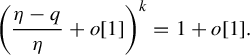 $$ \begin{align} \bigg(\frac{\eta-q}{\eta}+o[1]\bigg)^k=1+o[1]. \end{align} $$
Finally, keeping in mind $|k|_p\leq 1$
, from (4.4),
$|k|_p\leq 1$
, from (4.4),
 $$ \begin{align*}\bigg(\frac{\eta-q}{\eta}\bigg)^k=1+o[1]. \end{align*} $$
( $2_\eta $
) Let
$2_\eta $
) Let $|\eta |_p>|q|_p$
. First, let us assume that
$|\eta |_p>|q|_p$
. First, let us assume that $|k|_p\leq |\eta -k|_p$
. Then, using the strong triangle inequality, we can easily check
$|k|_p\leq |\eta -k|_p$
. Then, using the strong triangle inequality, we can easily check
 $$ \begin{align} \frac{k}{\eta}\neq1+o[1]. \end{align} $$
From $|\theta -1|_p<|q^2|_p$
and
$|\theta -1|_p<|q^2|_p$
and $|q|_p<|\eta |_p$
,
$|q|_p<|\eta |_p$
,
 $$ \begin{align*}g_{\theta,q}(x_\eta)=1-\frac{q}{\eta}+o[q]. \end{align*} $$
Keeping in mind $f_{\theta ,q,k}(x_\eta )=(g_{\theta ,q}(x_\eta ))^k$
, by (2.3),
$f_{\theta ,q,k}(x_\eta )=(g_{\theta ,q}(x_\eta ))^k$
, by (2.3),
 $$ \begin{align} f_{\theta,q,k}(x_\eta)=1-\frac{kq}{\eta}+o\bigg[\frac{kq}{\eta}\bigg]. \end{align} $$
Plugging (4.5) into (4.6) yields
 $$ \begin{align*}f_{\theta,q,k}(x_\eta)-1\neq-q+o[q], \end{align*} $$
but it contracts to $f_{\theta ,q,k}(x_\eta )-1+q=o[q]$
. This means that
$f_{\theta ,q,k}(x_\eta )-1+q=o[q]$
. This means that $|\eta |_p>|q|_p$
and (4.1) hold only for
$|\eta |_p>|q|_p$
and (4.1) hold only for $|\eta -k|_p<|k|_p$
.
$|\eta -k|_p<|k|_p$
.
So, suppose $|\eta -k|_p<|k|_p$
, which implies
$|\eta -k|_p<|k|_p$
, which implies $|\eta |_p=|k|_p$
. Now we prove our assertion by contradiction. Suppose in contrary,
$|\eta |_p=|k|_p$
. Now we prove our assertion by contradiction. Suppose in contrary,
 $$ \begin{align} \bigg|\eta-k+\frac{(k-1)q}{2}-\frac{(k-1)(k-2)q^2}{6k}\bigg|_p\geq|q|_p. \end{align} $$
Noting $|q|_p<|k|_p\leq 1$
, we then can easily check the following:
$|q|_p<|k|_p\leq 1$
, we then can easily check the following:
 $$ \begin{align*} &\bigg|\frac{(k-1)q}{2}\bigg|_p\leq|q|_p,\\ &\bigg|\frac{(k-1)(k-2)q^2}{6k}\bigg|_p\leq|q|_p. \end{align*} $$
These inequalities together with (4.7) yield
 $$ \begin{align} \bigg|\eta-k+\frac{(k-1)q}{2}-\frac{(k-1)(k-2)q^2}{6k}\bigg|_p=\max\{|\eta-k|_p, |q|_p\}. \end{align} $$
Owing to $|\theta -1|_p<|q^2|_p$
and
$|\theta -1|_p<|q^2|_p$
and $|\eta |_p=|k|_p$
, we have
$|\eta |_p=|k|_p$
, we have
 $$ \begin{align} f_{\theta,q,k}(x_\eta)&=\bigg(1-\frac{q}{\eta}+\frac{(\eta-1)(\theta-1)}{\eta}\bigg)^k\nonumber\\ &=\bigg(1-\frac{q}{\eta}+o\bigg[\frac{q^2}{k}\bigg]\bigg)^k\nonumber\\[-12pt] & \nonumber \\ &=\bigg(1-\frac{q}{\eta}\bigg)^k+o\bigg[\frac{q^2}{k}\bigg]\nonumber\\[2mm] &=\bigg(1-\frac{q}{k}\sum_{n=0}^\infty\bigg(\frac{k-\eta}{k}\bigg)^n\bigg)^k+o\bigg[\frac{q^2}{k}\bigg]\nonumber\\[2mm] &=1-q\sum_{n=0}^\infty\bigg(\frac{k-\eta}{k}\bigg)^n+\frac{(k-1)q^2}{2k}-\frac{(k-1)(k-2)q^3}{6k^2}+o\bigg[\frac{q^2}{k}\bigg]\nonumber\\[2mm] &=1-q+\frac{q}{k}\bigg(\eta-k+\frac{(k-1)q}{2}-\frac{(k-1)(k-2)q^2}{6k}\bigg)\nonumber\\ &\quad -q\sum_{n=2}^\infty\bigg(\frac{k-\eta}{k}\bigg)^n+o\bigg[\frac{q^2}{k}\bigg]. \end{align} $$
We calculate the norm of $q\sum _{n=2}^\infty (({k-\eta })/{k})^n.$
Keeping in mind
$q\sum _{n=2}^\infty (({k-\eta })/{k})^n.$
Keeping in mind $|\eta -k|_p<|k|_p$
, by the strong triangle inequality,
$|\eta -k|_p<|k|_p$
, by the strong triangle inequality,
 $$ \begin{align} \bigg|q\sum_{n=2}^\infty\bigg(\frac{k-\eta}{k}\bigg)^n\bigg|_p=\bigg|\frac{q(k-\eta)^2}{k^2}\bigg|_p. \end{align} $$
So, we need to calculate the norm of $({q(k-\eta )^2})/{k^2}$
. One can see that
$({q(k-\eta )^2})/{k^2}$
. One can see that
 $$ \begin{align*}\bigg|\frac{(k-\eta)^2}{k}\bigg|_p<|\eta-k|_p\leq\max\{|\eta-k|_p, |q|_p\}. \end{align*} $$
The last inequality together with (4.10) yields
 $$ \begin{align} \bigg|q\sum_{n=2}^\infty\bigg(\frac{k-\eta}{k}\bigg)^n\bigg|_p <\bigg|\frac{q}{k}\bigg|_p\cdot\max\{|\eta-k|_p, |q|_p\}. \end{align} $$
Then by (4.8) and (4.11), using the strong triangle inequality, one finds
 $$ \begin{align*} &\bigg|\frac{q}{k}\bigg(\eta-k+\frac{(k-1)q}{2}-\frac{(k-1)(k-2)q^2}{6k}\bigg) -q\sum_{n=2}^\infty\bigg(\frac{k-\eta}{k}\bigg)^n\bigg|_p\\&\qquad=\bigg|\frac{q}{k}\bigg|_p\cdot\max\{|\eta-k|_p,|q|_p\}. \end{align*} $$
From the last equality,
 $$ \begin{align} \bigg|\frac{q}{k}\bigg(\eta-k+\frac{(k-1)q}{2}-\frac{(k-1)(k-2)q^2}{6k}\bigg) -q\sum_{n=2}^\infty\bigg(\frac{k-\eta}{k}\bigg)^n\bigg|_p\geq\frac{|q^2|_p}{|k|_p}. \end{align} $$
Hence, plugging (4.12) into (4.9) and noting $|k|_p\leq 1$
, one finds
$|k|_p\leq 1$
, one finds
 $$ \begin{align*}|f_{\theta,q,k}(x_\eta)-1+q|_p\geq|q^2|_p, \end{align*} $$
which together with $|\theta -1|_p<|q^2|_p$
implies
$|\theta -1|_p<|q^2|_p$
implies $|f_{\theta ,q,k}(x_\eta )-2+q+\theta |_p>|\theta -1|_p$
, which contradicts (4.1). This means that if for
$|f_{\theta ,q,k}(x_\eta )-2+q+\theta |_p>|\theta -1|_p$
, which contradicts (4.1). This means that if for $|\eta |_p>|q|_p$
, (4.1) holds, then
$|\eta |_p>|q|_p$
, (4.1) holds, then
 $$ \begin{align*}\eta=k-\frac{(k-1)q}{2}+\frac{(k-1)(k-2)q^2}{6k}+o[q].\\[-42pt] \end{align*} $$
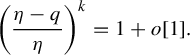
Remark 4.6. One can see that if $|\eta |_p=|q|_p$
and
$|\eta |_p=|q|_p$
and $(({\eta -q})/{\eta })^k\in \mathcal E_p$
, then
$(({\eta -q})/{\eta })^k\in \mathcal E_p$
, then $(({\eta -q})/{\eta })\in \mathbb Z_p^*\setminus \mathcal E_p$
. This means that there exists a root of unity
$(({\eta -q})/{\eta })\in \mathbb Z_p^*\setminus \mathcal E_p$
. This means that there exists a root of unity $\xi \neq 1$
such that
$\xi \neq 1$
such that $({\eta -q})/{\eta }=\xi +o[1]$
, which yields
$({\eta -q})/{\eta }=\xi +o[1]$
, which yields $\eta ={q}/({1-\xi })+o[q]$
. Without loss of generality for
$\eta ={q}/({1-\xi })+o[q]$
. Without loss of generality for $\xi =1$
, we put
$\xi =1$
, we put $\eta =k-(({(k-1)q})/{2})+(({(k-1)(k-2)q^2})/{6k})+o[q]$
. Consequently, we have found a relation between all roots of unity and all
$\eta =k-(({(k-1)q})/{2})+(({(k-1)(k-2)q^2})/{6k})+o[q]$
. Consequently, we have found a relation between all roots of unity and all $\eta \in \mathbb Q_p$
for which (4.1) holds.
$\eta \in \mathbb Q_p$
for which (4.1) holds.
Let us denote
 $$ \begin{align*}\mathrm{Sol}_p(x^k-1)=\{\xi\in\mathbb Z_p^*: \xi^k=1\},\ \ \ \kappa_p=\mathrm{card}(\mathrm{Sol}_p(x^k-1)), \end{align*} $$
where $\mathrm {card}(A)$
is the cardinality of a set A.
$\mathrm {card}(A)$
is the cardinality of a set A.
We point out that $\kappa _p$
is the number of solutions of the equation
$\kappa _p$
is the number of solutions of the equation $x^k=1$
in
$x^k=1$
in ${\mathbb Q}_p$
. From the results of [Reference Mukhamedov and Saburov38], we infer that
${\mathbb Q}_p$
. From the results of [Reference Mukhamedov and Saburov38], we infer that $\kappa _p$
is the GCF of k and
$\kappa _p$
is the GCF of k and $p-1$
. Therefore, it is clear that
$p-1$
. Therefore, it is clear that $1\leq \kappa _p\leq k$
.
$1\leq \kappa _p\leq k$
.
For a given $\xi _i\in \mathrm {Sol}_p(x^k-1),\ i\in \{1,\ldots ,\kappa _p\}$
, we define
$\xi _i\in \mathrm {Sol}_p(x^k-1),\ i\in \{1,\ldots ,\kappa _p\}$
, we define
 $$ \begin{align} {x}_{\xi_i}=\left\{ \begin{array}{@{}ll} 1-q+(k-1)\bigg(1-\dfrac{q}{2}+\dfrac{(k-2)q^2}{6k}\bigg)(\theta-1) & \text{if }\ \xi_i=1,\\[5mm] 2-q-\theta+\dfrac{q}{1-\xi_i}(\theta-1) & \text{if }\ \xi_i\neq1, \end{array}\right. \end{align} $$
and
 $$ \begin{align} X=\bigcup\limits_{i=1}^{\kappa_p}B_r({x}_{\xi_i}),\quad r=|q(\theta-1)|_p. \end{align} $$
By construction, the set X is a subset of $\mathcal E_p\setminus \{1\}$
.
$\mathcal E_p\setminus \{1\}$
.
Thanks to Remark 4.4, as a corollary of Proposition 4.5, we can formulate the following result which describes the basin of attraction of $x_0^*=1$
.
$x_0^*=1$
.
Proposition 4.7. Let $p\geq 3$
and
$p\geq 3$
and $|k|_p>|q|_p$
. If
$|k|_p>|q|_p$
. If $|\theta -1|_p<|q^2|_p$
, then
$|\theta -1|_p<|q^2|_p$
, then
 $$ \begin{align*}\lim\limits_{n\to\infty}f_{\theta,q,k}^n(x)=1 \quad\text{for all } x\in \mathrm{Dom}(f_{\theta,q,k})\setminus X. \end{align*} $$
The next result shows that the set X (given by (4.14)) consists of disjoint balls.
Lemma 4.8. Let $p\geq 3$
and
$p\geq 3$
and $|\theta -1|_p<|q^2|_p<|k^2|_p$
. If
$|\theta -1|_p<|q^2|_p<|k^2|_p$
. If $x_{\xi _i}$
is given by (4.13) and
$x_{\xi _i}$
is given by (4.13) and $r=|q(\theta -1)|_p$
, then
$r=|q(\theta -1)|_p$
, then $B_r({x}_{\xi _i})\cap B_r({x}_{\xi _j})=\varnothing $
if
$B_r({x}_{\xi _i})\cap B_r({x}_{\xi _j})=\varnothing $
if $i\neq j$
.
$i\neq j$
.
Proof. Let $x_{\xi _i}$
and
$x_{\xi _i}$
and $x_{\xi _j}$
be given by (4.13), where
$x_{\xi _j}$
be given by (4.13), where $i\neq j$
. We consider two cases.
$i\neq j$
. We consider two cases.
Case $\xi _i=1$
and
$\xi _i=1$
and $\xi _j\neq 1$
. Then from (4.13),
$\xi _j\neq 1$
. Then from (4.13),
 $$ \begin{align*} x_{\xi_i}-x_{\xi_j}&=\bigg(k-\frac{(k-1)q}{2}+\frac{(k-1)(k-2)q^2}{6k}-\frac{q}{1-\xi_j}\bigg)(\theta-1)\\[2mm] &=(k+o[k])(\theta-1)\\[2mm] &=O[k(\theta-1)], \end{align*} $$
which implies that $|x_{\xi _i}-x_{\xi _j}|_p>|q(\theta -1)|_p$
. Hence,
$|x_{\xi _i}-x_{\xi _j}|_p>|q(\theta -1)|_p$
. Hence, $B_r({x}_{\xi _i})\cap B_r({x}_{\xi _j})=\varnothing $
.
$B_r({x}_{\xi _i})\cap B_r({x}_{\xi _j})=\varnothing $
.
Case $\xi _i\neq 1$
and
$\xi _i\neq 1$
and $\xi _j\neq 1$
. In this case,
$\xi _j\neq 1$
. In this case,
 $$ \begin{align*}x_{\xi_i}-x_{\xi_j}=\frac{(\xi_i-\xi_j)q(\theta-1)}{(1-\xi_i)(1-\xi_j)} =\frac{O[1]q(\theta-1)}{O[1]} =O[q(\theta-1)], \end{align*} $$
which means $|x_{\xi _i}-x_{\xi _j}|_p=r$
. Hence, we infer that
$|x_{\xi _i}-x_{\xi _j}|_p=r$
. Hence, we infer that $B_r({x}_{\xi _i})\cap B_r({x}_{\xi _j})=\varnothing $
.
$B_r({x}_{\xi _i})\cap B_r({x}_{\xi _j})=\varnothing $
.
To prove the first part of (B) of Theorem 1.1, we define the following set:
 $$ \begin{align} J_{f_{\theta,q,k}}=\bigcap\limits_{n=1}^\infty f_{\theta,q,k}^{-n}(X). \end{align} $$
Remark 4.9. In [Reference Mukhamedov and Khakimov36], we have considered the following function over $\mathbb Q_p$
(
$\mathbb Q_p$
( $p\geq 3$
):
$p\geq 3$
):
 $$ \begin{align*}f_{b,c,d}(x)=\bigg(\frac{bx-c}{x-d}\bigg)^k,\quad b,c,d\in\mathcal E_p,\ c\neq bd. \end{align*} $$
It was proved that the mapping $f_{b,c,d}$
has exactly
$f_{b,c,d}$
has exactly $\kappa _p+1$
fixed points belonging to
$\kappa _p+1$
fixed points belonging to $\mathcal E_p$
if
$\mathcal E_p$
if $d=1-b+c$
and
$d=1-b+c$
and $|b-1|_p<|c-1|_p^2<|k|_p^2$
(see [Reference Mukhamedov and Khakimov36, Theorem 4.5]). One can see that if one takes
$|b-1|_p<|c-1|_p^2<|k|_p^2$
(see [Reference Mukhamedov and Khakimov36, Theorem 4.5]). One can see that if one takes $b=\theta $
,
$b=\theta $
, $c=1-q$
, and
$c=1-q$
, and $d=2-q-\theta $
, then the function
$d=2-q-\theta $
, then the function $f_{b,c,d}$
reduces to
$f_{b,c,d}$
reduces to $f_{\theta ,q,k}$
. So, as a corollary of the mentioned result and noting that
$f_{\theta ,q,k}$
. So, as a corollary of the mentioned result and noting that $\mathrm{Fix}(f_{\theta ,q,k})\cap (\mathbb Q_p\setminus X)=\{1\}$
, we conclude that if
$\mathrm{Fix}(f_{\theta ,q,k})\cap (\mathbb Q_p\setminus X)=\{1\}$
, we conclude that if $|\theta -1|_p<|q|_p^2<|k|_p^2$
, then
$|\theta -1|_p<|q|_p^2<|k|_p^2$
, then $f_{\theta ,q,k}$
has exactly
$f_{\theta ,q,k}$
has exactly $\kappa _p$
fixed points belonging to X. This yields
$\kappa _p$
fixed points belonging to X. This yields $J_{f_{\theta ,q,k}}\neq \varnothing $
for
$J_{f_{\theta ,q,k}}\neq \varnothing $
for $|\theta -1|_p<|q|_p^2<|k|_p^2$
. Moreover, we may check that for every
$|\theta -1|_p<|q|_p^2<|k|_p^2$
. Moreover, we may check that for every $i\in \{1,2,\ldots ,\kappa _p\}$
, there exists a unique fixed point of
$i\in \{1,2,\ldots ,\kappa _p\}$
, there exists a unique fixed point of $f_{\theta ,q,k}$
in
$f_{\theta ,q,k}$
in $B_r(x_{\xi _i})$
(see Proposition 5.5).
$B_r(x_{\xi _i})$
(see Proposition 5.5).
Proof of Theorem 1.1: (B)
By Proposition 4.7, the set $\mathcal P_{x^{(\infty )}}$
can not belong to
$\mathcal P_{x^{(\infty )}}$
can not belong to $\mathrm{Dom}(f_{\theta ,q,k})\setminus X$
. Then
$\mathrm{Dom}(f_{\theta ,q,k})\setminus X$
. Then $\mathcal P_{x^{(\infty )}}\subset X$
. According to the construction of
$\mathcal P_{x^{(\infty )}}\subset X$
. According to the construction of $J_{f_{\theta ,q,k}}$
(see (4.15)), we conclude that
$J_{f_{\theta ,q,k}}$
(see (4.15)), we conclude that $J_{f_{\theta ,q,k}}\cap \mathcal P_{x^{(\infty )}}=\varnothing $
. However, owing to Remark 4.9, the set
$J_{f_{\theta ,q,k}}\cap \mathcal P_{x^{(\infty )}}=\varnothing $
. However, owing to Remark 4.9, the set $J_{f_{\theta ,q,k}}$
is not empty and by the construction, it is invariant with respect to
$J_{f_{\theta ,q,k}}$
is not empty and by the construction, it is invariant with respect to $f_{\theta ,q,k}$
. Then for any
$f_{\theta ,q,k}$
. Then for any $x\not \in J_{f_{\theta ,q,k}}\cup \mathcal P_{x^{(\infty )}}$
, there exists a number
$x\not \in J_{f_{\theta ,q,k}}\cup \mathcal P_{x^{(\infty )}}$
, there exists a number $m\geq 1$
such that
$m\geq 1$
such that $f_{\theta ,q,k}^m(x)\not \in X$
. Hence, owing to Proposition 4.7, we infer that
$f_{\theta ,q,k}^m(x)\not \in X$
. Hence, owing to Proposition 4.7, we infer that $f_{\theta ,q,k}^n(x)\to 1$
as
$f_{\theta ,q,k}^n(x)\to 1$
as $n\to \infty $
. The proof is complete.
$n\to \infty $
. The proof is complete.
5 Proof of Theorem 1.1: parts (B1) and (B2)
In the following, we need some auxiliary facts.
Lemma 5.1. Let $p\geq 3$
and
$p\geq 3$
and $|k|_p>|q|_p$
. Then for any
$|k|_p>|q|_p$
. Then for any $a\in B_{|q^2|_p}(1-q)$
, the equation
$a\in B_{|q^2|_p}(1-q)$
, the equation $x^k=a$
has a unique solution
$x^k=a$
has a unique solution $x_*$
on
$x_*$
on $\mathcal E_p$
. Moreover, this solution satisfies
$\mathcal E_p$
. Moreover, this solution satisfies
 $$ \begin{align} x_*-1+\frac{q}{k}+\frac{(k-1)q^2}{2k^2}-\frac{(k-1)(k-2)q^3}{6k^3}=o\bigg[\frac{q^2}{k^2}\bigg]. \end{align} $$
Proof. Let $|k|_p>|q|_p$
and
$|k|_p>|q|_p$
and $a\in B_{|q^2|_p}(1-q)$
. For convenience, we use the canonical form of a:
$a\in B_{|q^2|_p}(1-q)$
. For convenience, we use the canonical form of a:
 $$ \begin{align*}a=1+a_tp^t+a_{t+1}p^{t+1}+\cdots \end{align*} $$
We note that $|k|_p>p^{-t}$
. Let us put
$|k|_p>p^{-t}$
. Let us put $x_t=1$
and define a sequence
$x_t=1$
and define a sequence $\{x_{n+t-1}\}_{n\geq 1}$
as follows:
$\{x_{n+t-1}\}_{n\geq 1}$
as follows:
 $$ \begin{align} x_{n+t}=x_{n+t-1}+\frac{a-x_{n+t-1}^k}{k}. \end{align} $$
First, by induction, let us show that $x_{n+t-1}\in \mathcal E_p$
for any
$x_{n+t-1}\in \mathcal E_p$
for any $n\geq 1$
. It is clear that
$n\geq 1$
. It is clear that $x_t\in \mathcal E_p$
and, therefore, we assume that
$x_t\in \mathcal E_p$
and, therefore, we assume that $x_{n+t-1}\in \mathcal E_p$
for some
$x_{n+t-1}\in \mathcal E_p$
for some $n\geq 1$
. Then, owing to Remark 2.7, we obtain
$n\geq 1$
. Then, owing to Remark 2.7, we obtain
 $$ \begin{align*}x_{n+t-1}^k-1=k(x_{n+t-1}-1)+o[k(x_{n+t-1}-1)], \end{align*} $$
which is equivalent to
 $$ \begin{align*}|x_{n+t-1}^k-1|_p<|k|_p. \end{align*} $$
The last inequality together with $|a-1|_p<|k|_p$
implies that
$|a-1|_p<|k|_p$
implies that $|x_{n+t}-x_{n+t-1}|_p<1$
. Consequently, from
$|x_{n+t}-x_{n+t-1}|_p<1$
. Consequently, from $x_{n+t-1}\in \mathcal E_p$
, we find
$x_{n+t-1}\in \mathcal E_p$
, we find $x_{n+t}\in \mathcal E_p$
. Hence,
$x_{n+t}\in \mathcal E_p$
. Hence, $x_{n+t}\in \mathcal E_p$
for any
$x_{n+t}\in \mathcal E_p$
for any $n\geq 1$
.
$n\geq 1$
.
Owing to Corollary 2.6, by (5.2), we have
 $$ \begin{align*} x_{n+t}^k-x_{n+t-1}^k&=k(x_{n+t}-x_{n+t-1})+o[k(x_{n+t}-x_{n+t-1})]\\ &=a-x_{n+t-1}^k+o[a-x_{n+t-1}], \end{align*} $$
which means
 $$ \begin{align*}|x_{n+t}^k-a|_p<|x_{n+t-1}^k-a|_p. \end{align*} $$
Hence, there exists a number $n_0\geq 1$
such that
$n_0\geq 1$
such that
 $$ \begin{align*}|x_{n_0+t}^k-a|_p\leq|(a-1)^2|_p.\end{align*} $$
Now, let us consider a polynomial $F(x)=x^k-a$
. It is easy to check that
$F(x)=x^k-a$
. It is easy to check that
 $$ \begin{align*}|F'(x_{n_0+t-1})|_p=|k|_p, \quad \text{and} \quad |F(x_{n_0+t-1})|_p\leq|(a-1)^2|_p.\end{align*} $$
So by $|k^2|_p>|(a-1)^2|_p$
and Hensel’s lemma, we conclude that F has a root
$|k^2|_p>|(a-1)^2|_p$
and Hensel’s lemma, we conclude that F has a root $x_*$
such that
$x_*$
such that
 $$ \begin{align*}|x_*-x_{n_0+t-1}|_p\leq|(a-1)^2|_p.\end{align*} $$
From $x_{n_0+t-1}\in \mathcal E_p$
, we infer that
$x_{n_0+t-1}\in \mathcal E_p$
, we infer that $x_*\in \mathcal E_p$
. The uniqueness of the solution on
$x_*\in \mathcal E_p$
. The uniqueness of the solution on $\mathcal E_p$
immediately follows from Remark 2.7.
$\mathcal E_p$
immediately follows from Remark 2.7.
Suppose that $x_*\in \mathcal E_p$
is a solution of
$x_*\in \mathcal E_p$
is a solution of $x^k-a=0$
. Let us show that it can be represented by (5.1). It can be checked that
$x^k-a=0$
. Let us show that it can be represented by (5.1). It can be checked that $x_*$
has the following form:
$x_*$
has the following form:
 $$ \begin{align} x_*=1-\frac{q}{k}+\alpha_*, \end{align} $$
where $\alpha _*=o[{q}/{k}]$
. Indeed, because
$\alpha _*=o[{q}/{k}]$
. Indeed, because $x_*\in \mathcal E_p$
, there exists
$x_*\in \mathcal E_p$
, there exists $y_*\in p\mathbb Z_p$
such that
$y_*\in p\mathbb Z_p$
such that $x_*$
can be represented as follows:
$x_*$
can be represented as follows: $x_*=1+y_*+o[y_*]$
. Then by Remark 2.7, we have
$x_*=1+y_*+o[y_*]$
. Then by Remark 2.7, we have $x_*^k=1+ky_*+o[ky_*]$
. By assumption,
$x_*^k=1+ky_*+o[ky_*]$
. By assumption, $a=1-q+o[q^2]$
. Hence, we obtain the following implications:
$a=1-q+o[q^2]$
. Hence, we obtain the following implications:
 $$ \begin{align*}x_*^k-a=0&\ \ \ \Longrightarrow\ \ \ ky_*+q=o[q]\ \ \ \Longrightarrow\ \ \ y_*=-\frac{q}{k}+o\bigg[\frac{q}{k}\bigg] \\ &\ \ \ \Longrightarrow\ \ \ x_*=1-\frac{q}{k}+o\bigg[\frac{q}{k}\bigg]. \end{align*} $$
Furthermore, from (5.3), one finds
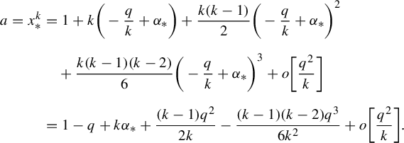 $$ \begin{align*} a=x_*^k&=1+k\bigg(-\frac{q}{k}+\alpha_*\bigg)+\frac{k(k-1)}{2}\bigg(-\frac{q}{k}+\alpha_*\bigg)^2\\[2mm] &\quad +\frac{k(k-1)(k-2)}{6} \bigg(-\frac{q}{k}+\alpha_*\bigg)^3+o\bigg[\frac{q^2}{k}\bigg]\\[2mm] &=1-q+k\alpha_*+\frac{(k-1)q^2}{2k}-\frac{(k-1)(k-2)q^3}{6k^2}+o\bigg[\frac{q^2}{k}\bigg]. \end{align*} $$
Plugging $a=1-q+o[q^2]$
into the last equality,
$a=1-q+o[q^2]$
into the last equality,
 $$ \begin{align*}k\alpha_*+\frac{(k-1)q^2}{2k}-\frac{(k-1)(k-2)q^3}{6k^2}=o\bigg[\frac{q^2}{k}\bigg]. \end{align*} $$
Hence,
 $$ \begin{align*}\alpha_*=-\frac{(k-1)q^2}{2k^2}+\frac{(k-1)(k-2)q^3}{6k^3}+o\bigg[\frac{q^2}{k^2}\bigg]. \end{align*} $$
Putting the last one into (5.3) yields (5.1), which completes the proof.
Remark 5.2. We point out that in [Reference Mukhamedov and Saburov38], the existence of solutions of the equation $x^k=a$
on
$x^k=a$
on $\mathbb Z^*_p$
has been obtained, but an advantage of Lemma 5.1 is that it provides the uniqueness of solution in
$\mathbb Z^*_p$
has been obtained, but an advantage of Lemma 5.1 is that it provides the uniqueness of solution in ${\mathcal E}_p$
with an explicit expression which is essential in our investigation.
${\mathcal E}_p$
with an explicit expression which is essential in our investigation.
On the set X (see (4.14)), the mapping $f_{\theta ,q,k}$
has exactly
$f_{\theta ,q,k}$
has exactly $\kappa _p$
inverse branches:
$\kappa _p$
inverse branches:
 $$ \begin{align*}h_{i}(x)=\frac{(q+\theta-2)\xi_i\sqrt[k]{x}-q+1}{\theta-\xi_i\sqrt[k]{x}}, \end{align*} $$
where $\xi _i^k=1$
,
$\xi _i^k=1$
, $i\in \{1,\ldots ,\kappa _p\}$
and
$i\in \{1,\ldots ,\kappa _p\}$
and $\sqrt [k]{x}$
, as before, is a principal root of
$\sqrt [k]{x}$
, as before, is a principal root of $x\in X$
(see Remark 2.9).
$x\in X$
(see Remark 2.9).
Proposition 5.3. Let $p\geq 3$
and
$p\geq 3$
and $|k|_p>|q|_p$
. If
$|k|_p>|q|_p$
. If $|\theta -1|_p<|q^2|_p$
, then
$|\theta -1|_p<|q^2|_p$
, then
 $$ \begin{align} h_{i}(X)\subset B_r(x_{\xi_i}). \end{align} $$
Proof. Let $x\in X$
. We consider two cases:
$x\in X$
. We consider two cases: $\xi _i=1$
and
$\xi _i=1$
and $\xi _i\neq 1$
.
$\xi _i\neq 1$
.
Case $\xi _i=1$
. In this case, we have
$\xi _i=1$
. In this case, we have
 $$ \begin{align} &h_{i}(x)-x_{\xi_i}\nonumber\\&=\frac{(q+\theta-2)\sqrt[k]{x}-q+1}{\theta-\sqrt[k]{x}}- \bigg(1-q+(k-1)\bigg(1-\frac{q}{2}+\frac{(k-2)q^2}{6k}\bigg)(\theta-1)\bigg)\nonumber\\[2mm] &=\frac{(\theta-1)(q+\theta-1+(k-(({(k-1)q})/{2})+(({(k-1)(k-2)q^2})/{6k}))(\sqrt[k]{x}-\theta))}{\theta-\sqrt[k]{x}}\nonumber\\[2mm] &=\frac{(\theta-1)(q+(k-(({(k-1)q})/{2})+(({(k-1)(k-2)q^2})/{6k}))(\sqrt[k]{x}-1)+o[q^2])}{1-\sqrt[k]{x}+o[q^2]}. \end{align} $$
However, owing to Lemma 5.1,
 $$ \begin{align} \sqrt[k]{x}-1=-\frac{q}{k}-\frac{(k-1)q^2}{2k^2}+\frac{(k-1)(k-2)q^3}{6k^3}+o\bigg[\frac{q^2}{k^2}\bigg]. \end{align} $$
Furthermore, keeping in mind $|q|_p<|k|_p$
, we can easily check the following:
$|q|_p<|k|_p$
, we can easily check the following:
 $$ \begin{align} q+\bigg(k-\frac{(k-1)q}{2}+\frac{(k-1)(k-2)q^2}{6k}\bigg)(\sqrt[k]{x}-1)=o\bigg[\frac{q^2}{k}\bigg]. \end{align} $$
Plugging (5.6), (5.7) into (5.5), one has
 $$ \begin{align*}h_{i}(x)-x_{\xi_i}= \frac{(\theta-1)o[{q^2}/{k}]}{O[{q}/{k}]} =(\theta-1)o[q] =o[q(\theta-1)]. \end{align*} $$
This means $h_{i}(x)\in B_r(x_{\xi _i})$
. The arbitrariness of
$h_{i}(x)\in B_r(x_{\xi _i})$
. The arbitrariness of $x\in X$
yields (5.4).
$x\in X$
yields (5.4).
Case $\xi _i\neq 1$
. Then,
$\xi _i\neq 1$
. Then,
 $$ \begin{align*} h_{i}(x)-x_{\xi_i}&=\frac{(q+\theta-2)\xi_i\sqrt[k]{x}-q+1}{\theta-\xi_i\sqrt[k]{x}}-\bigg(2-q-\theta+\frac{q}{1-\xi_i}(\theta-1)\bigg)\\[2mm] &=\frac{(\theta-1)(q-({\theta q}/({1-\xi_i}))+({\xi_i\sqrt[k]{x}q}/({1-\xi_i}))+\theta-1)}{\theta-1+1-\xi_i\sqrt{x}}\\[2mm] &=\frac{(\theta-1)(q-({q}/({1-\xi_i}))+({\xi_iq}/({1-\xi_i}))+o[q])}{O[1]}\\[2mm] &=\frac{(\theta-1)o[q]}{O[1]}\\[2mm] &=o[q(\theta-1)]. \end{align*} $$
The last one implies $h_{i}(x)\in B_r(x_{\xi _i})$
. Again, owing to the arbitrariness of
$h_{i}(x)\in B_r(x_{\xi _i})$
. Again, owing to the arbitrariness of $x\in X$
, we obtain (5.4).
$x\in X$
, we obtain (5.4).
Corollary 5.4. Let $p\geq 3$
and
$p\geq 3$
and $|k|_p>|q|_p$
. If
$|k|_p>|q|_p$
. If $|\theta -1|_p<|q^2|_p$
and X is the set given by (4.14), then the following statements hold:
$|\theta -1|_p<|q^2|_p$
and X is the set given by (4.14), then the following statements hold:
-
(i)
$f_{\theta ,q,k}^{-1}(X)\subset X$
; -
(ii)
$B_r({x}_{\xi _i})\subset f_{\theta ,q,k}(B_{r}(x_{\xi _j}))$
for any
$i,j\in \{1,\ldots ,\kappa _p\}$
.


Proposition 5.5. Let $p\geq 3$
,
$p\geq 3$
, $|k|_p>|q|_p$
. If
$|k|_p>|q|_p$
. If $|\theta -1|_p<|q^2|_p$
and X is the set given by (4.14), then the following statements hold:
$|\theta -1|_p<|q^2|_p$
and X is the set given by (4.14), then the following statements hold:
-
(a) if
$\xi _i=1$
, then (5.8)
$$ \begin{align} |f_{\theta,q,k}(x)-f_{\theta,q,k}(y)|_p=\frac{|q(x-y)|_p}{|k(\theta-1)|_p}\quad \text{for any }x,y\in B_r(x_{\xi_i}); \end{align} $$
-
(b) if
$\xi _i\neq 1$
, then (5.9)
$$ \begin{align} |f_{\theta,q,k}(x)-f_{\theta,q,k}(y)|_p=\frac{|k(x-y)|_p}{|q(\theta-1)|_p}\quad \text{for any }x,y\in B_r(x_{\xi_i}). \end{align} $$


Proof. (a) Recall that for $\xi _i=1$
,
$\xi _i=1$
,
 $$ \begin{align*}x_{\xi_i}=1-q+(k-1)\bigg(1-\frac{q}{2}+\frac{(k-2)q^2}{6k}\bigg)(\theta-1). \end{align*} $$
Thus for $x\in B_r(x_{\xi _i})$
, by (3.2), we have
$x\in B_r(x_{\xi _i})$
, by (3.2), we have
 $$ \begin{align*}g_{\theta,q}(x)-1=\frac{(\theta-1)(-q+o[q])}{k(\theta-1)+o[k(\theta-1)]} =O\bigg[\frac{q}{k}\bigg]. \end{align*} $$
This means $g_{\theta ,q}(x)\in \mathcal E_p$
. Then, owing to Corollary 2.6, for any
$g_{\theta ,q}(x)\in \mathcal E_p$
. Then, owing to Corollary 2.6, for any $x,y\in B_r(x_{\xi _i})$
,
$x,y\in B_r(x_{\xi _i})$
,
 $$ \begin{align} |f_{\theta,q,k}(x)-f_{\theta,q,k}(y)|_p=|k(g_{\theta,q}(x)-g_{\theta,q}(y))|_p. \end{align} $$
However,
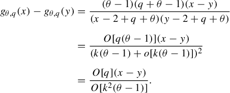 $$ \begin{align*} g_{\theta,q}(x)-g_{\theta,q}(y)&=\frac{(\theta-1)(q+\theta-1)(x-y)}{(x-2+q+\theta)(y-2+q+\theta)}\\[2mm] &=\frac{O[q(\theta-1)](x-y)}{(k(\theta-1)+o[k(\theta-1)])^2}\\[2mm] &=\frac{O[q](x-y)}{O[k^2(\theta-1)]}. \end{align*} $$
Plugging the last one into (5.10) implies (5.8).
(b) Recall that for $\xi _i\neq 1$
,
$\xi _i\neq 1$
,
 $$ \begin{align*}x_{\xi_i}=2-q-\theta+\frac{q(\theta-1)}{1-\xi_i}. \end{align*} $$
Then for $x\in B_r(x_{\xi _i})$
,
$x\in B_r(x_{\xi _i})$
,
 $$ \begin{align*}g_{\theta,q}(x)=1+\frac{(\theta-1)(x-1)}{x-2+q+\theta} =1+\frac{(\theta-1)(-q+o[q])}{({q(\theta-1)})/({1-\xi_i})+o[q(\theta-1)]} =\xi_i+o[1]. \end{align*} $$
So, $|g_{\theta ,q}(x)|_p=1$
. Moreover,
$|g_{\theta ,q}(x)|_p=1$
. Moreover, $({g_{\theta ,q}(x)}/{g_{\theta ,q}(y)})\in \mathcal E_p$
for any
$({g_{\theta ,q}(x)}/{g_{\theta ,q}(y)})\in \mathcal E_p$
for any $x,y\in B_r(x_{\xi _i})$
. Then, owing to Corollary 2.6,
$x,y\in B_r(x_{\xi _i})$
. Then, owing to Corollary 2.6,
 $$ \begin{align} |f_{\theta,q,k}(x)-f_{\theta,q,k}(y)|_p=|k(g_{\theta,q}(x)-g_{\theta,q}(y))|_p. \end{align} $$
However, from
 $$ \begin{align*} g_{\theta,q}(x)-g_{\theta,q}(y)&=\frac{(\theta-1)(q+\theta-1)(x-y)}{(x-2+q+\theta)(y-2+q+\theta)}\\[2mm] &=\frac{O[q(\theta-1)](x-y)}{(({q(\theta-1)})/({1-\xi_i})+o[q(\theta-1)])^2}\\[2mm] &=\frac{(x-y)}{O[q(\theta-1)]} \end{align*} $$
Proof of Theorem 1.1
(B1) Assume that $x^k=1$
has only one solution. Then the set X given by (4.14) consists of only one ball
$x^k=1$
has only one solution. Then the set X given by (4.14) consists of only one ball $B_r(x_1)$
, where
$B_r(x_1)$
, where
 $$ \begin{align*}x_1=1-q+(k-1)\bigg(1-\frac{q}{2}\bigg)(\theta-1),\quad r=|q(\theta-1)|_p. \end{align*} $$
By the proof for the case (B),
 $$ \begin{align*}A(x_0^*)=\mathrm{Dom}(f_{\theta,q,k})\setminus(J_{f_{\theta,q,k}}\cup\mathcal P_{x^{(\infty)}}), \end{align*} $$
where $x_0^*=1$
, and
$x_0^*=1$
, and $J_{f_{\theta ,q,k}}$
is given by (4.15). By Proposition 5.5, for any
$J_{f_{\theta ,q,k}}$
is given by (4.15). By Proposition 5.5, for any $x,y\in B_r(x_1)$
, we have
$x,y\in B_r(x_1)$
, we have
 $$ \begin{align*}|f_{\theta,q,k}(x)-f_{\theta,q,k}(y)|_p>p^2|x-y|_p, \end{align*} $$
which implies that $|J_{f_{\theta ,q,k}}|\leq 1$
. Thanks to Remark 4.9, we have
$|J_{f_{\theta ,q,k}}|\leq 1$
. Thanks to Remark 4.9, we have $J_{f_{\theta ,q,k}}\neq \varnothing $
. Because
$J_{f_{\theta ,q,k}}\neq \varnothing $
. Because $|J_{f_{\theta ,q,k}}|\leq 1$
, one has
$|J_{f_{\theta ,q,k}}|\leq 1$
, one has $J_{f_{\theta ,q,k}}=\{x_*\}$
, where
$J_{f_{\theta ,q,k}}=\{x_*\}$
, where $x_*\in \mathrm{Fix}(f_{\theta ,q,k})\cap (\mathcal E_p\setminus \{1\})$
.
$x_*\in \mathrm{Fix}(f_{\theta ,q,k})\cap (\mathcal E_p\setminus \{1\})$
.
(B2) Assume that $x^k=1$
has
$x^k=1$
has $\kappa _p$
(
$\kappa _p$
( $\kappa _p\geq 2$
) solutions. Consider the set X defined by (4.14). Then according to Corollary 5.4(i) and Proposition 5.5, the triple
$\kappa _p\geq 2$
) solutions. Consider the set X defined by (4.14). Then according to Corollary 5.4(i) and Proposition 5.5, the triple $(X,J_{f_{\theta ,q,k}},f_{\theta ,q,k})$
is a p-adic repeller. Owing to Corollary 5.4(ii), the corresponding incidence matrix A has dimension
$(X,J_{f_{\theta ,q,k}},f_{\theta ,q,k})$
is a p-adic repeller. Owing to Corollary 5.4(ii), the corresponding incidence matrix A has dimension $\kappa _p\times \kappa _p$
and can be written as follows:
$\kappa _p\times \kappa _p$
and can be written as follows:
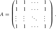 $$ \begin{align*}A=\left(\begin{array}{@{}llll} 1 & 1 & \cdots & 1\\ 1 & 1 & \cdots & 1\\ \vdots & \vdots & \ddots & \vdots\\ 1 & 1 & \cdots & 1 \end{array} \right). \end{align*} $$
This means that the triple $(X,J_{f_{\theta ,q,k}},f_{\theta ,q,k})$
is transitive. Hence, Theorem 2.10 implies that the dynamics
$(X,J_{f_{\theta ,q,k}},f_{\theta ,q,k})$
is transitive. Hence, Theorem 2.10 implies that the dynamics $(J_{f_{\theta ,q,k}},f_{\theta ,q,k},|\cdot |_p)$
is topologically conjugate to the full shift dynamics on
$(J_{f_{\theta ,q,k}},f_{\theta ,q,k},|\cdot |_p)$
is topologically conjugate to the full shift dynamics on $\kappa _p$
symbols.
$\kappa _p$
symbols.
Acknowledgments
The present work is supported by the UAEU UPAR Grant No. G00003247 (Fund No. 31S391). We are grateful to an anonymous referee whose useful suggestions and comments allowed us to improve the presentation of this paper.
A Appendix
A.1 p-adic measure
Let $(X,{\mathcal B})$
be a measurable space, where
$(X,{\mathcal B})$
be a measurable space, where ${\mathcal B}$
is an algebra of subsets X. A function
${\mathcal B}$
is an algebra of subsets X. A function $\mu :{\mathcal B}\to {\mathbb Q}_p$
is said to be a p-adic measure if for any
$\mu :{\mathcal B}\to {\mathbb Q}_p$
is said to be a p-adic measure if for any $A_1,\ldots ,A_n\subset {\mathcal B}$
such that
$A_1,\ldots ,A_n\subset {\mathcal B}$
such that $A_i\cap A_j=\varnothing $
(
$A_i\cap A_j=\varnothing $
( $i\neq j$
), the equality holds
$i\neq j$
), the equality holds
 $$ \begin{align*}\mu\bigg(\bigcup_{j=1}^{n} A_j\bigg)=\sum_{j=1}^{n}\mu(A_j). \end{align*} $$
A p-adic measure is called a probability measure if $\mu (X)=1$
. A p-adic probability measure
$\mu (X)=1$
. A p-adic probability measure $\mu $
is called bounded if
$\mu $
is called bounded if $\sup \{|\mu (A)|_p : A\in {\mathcal B}\}<\infty $
. For more detailed information about p-adic measures, we refer to [Reference Khrennikov19–Reference Khrennikov and Nilsson21].
$\sup \{|\mu (A)|_p : A\in {\mathcal B}\}<\infty $
. For more detailed information about p-adic measures, we refer to [Reference Khrennikov19–Reference Khrennikov and Nilsson21].
A.2 Cayley tree
Let $\Gamma ^k_+ = (V,L)$
be a semi-infinite Cayley tree of order
$\Gamma ^k_+ = (V,L)$
be a semi-infinite Cayley tree of order $k\geq 1$
with the root
$k\geq 1$
with the root $x^0$
(whose each vertex has exactly
$x^0$
(whose each vertex has exactly $k+1$
edges, except for the root
$k+1$
edges, except for the root $x^0$
, which has k edges). Here, V is the set of vertices and L is the set of edges. The vertices x and y are called nearest neighbors and they are denoted by
$x^0$
, which has k edges). Here, V is the set of vertices and L is the set of edges. The vertices x and y are called nearest neighbors and they are denoted by $l=\langle x,y\rangle $
if there exists an edge connecting them. A collection of the pairs
$l=\langle x,y\rangle $
if there exists an edge connecting them. A collection of the pairs $\langle x,x_1\rangle ,\ldots ,\langle x_{d-1},y\rangle $
is called a path from the point x to the point y. The distance
$\langle x,x_1\rangle ,\ldots ,\langle x_{d-1},y\rangle $
is called a path from the point x to the point y. The distance $d(x,y)$
,
$d(x,y)$
, $x,y\in V$
, on the Cayley tree, is the length of the shortest path from x to y.
$x,y\in V$
, on the Cayley tree, is the length of the shortest path from x to y.
 $$ \begin{align*}W_{n}=\{ x\in V\mid d(x,x^{0})=n\}, \quad V_n=\overset{n}{\underset{m=0}{\bigcup}}W_{m}, \quad L_{n}=\{ l=\langle x,y\rangle\in L\mid x,y\in V_{n}\}. \end{align*} $$
The set of direct successors of x is defined by
 $$ \begin{align*}S(x)=\{ y\in W_{n+1}:d(x,y)=1\},\quad x\in W_{n}. \end{align*} $$
Observe that any vertex x has k direct successors.
A.3 p-adic quasi-Gibbs measure
In this section, we recall the definition of p-adic quasi-Gibbs measure (see [Reference Mukhamedov25]).
Let $q\geq 2$
and
$q\geq 2$
and $\Phi =\{1,2,\ldots ,q\}$
. Here,
$\Phi =\{1,2,\ldots ,q\}$
. Here, $\Phi $
is called a state space and is assigned to the vertices of the tree
$\Phi $
is called a state space and is assigned to the vertices of the tree $\Gamma ^k_+=(V,\Lambda )$
. A configuration
$\Gamma ^k_+=(V,\Lambda )$
. A configuration $\sigma $
on V is then defined as a function
$\sigma $
on V is then defined as a function $x\in V\to \sigma (x)\in \Phi $
; in a similar manner, one defines configurations
$x\in V\to \sigma (x)\in \Phi $
; in a similar manner, one defines configurations $\sigma _n$
and
$\sigma _n$
and $\omega $
on
$\omega $
on $V_n$
and
$V_n$
and $W_n$
. The set of all configurations on V (respectively
$W_n$
. The set of all configurations on V (respectively $V_n$
,
$V_n$
, $W_n$
) coincides with
$W_n$
) coincides with $\Omega =\Phi ^{V}$
(respectively
$\Omega =\Phi ^{V}$
(respectively $\Omega _{V_n}=\Phi ^{V_n},\ \ \Omega _{W_n}=\Phi ^{W_n}$
). One can see that
$\Omega _{V_n}=\Phi ^{V_n},\ \ \Omega _{W_n}=\Phi ^{W_n}$
). One can see that $\Omega _{V_n}=\Omega _{V_{n-1}}\times \Omega _{W_n}$
. Using this, for given configurations
$\Omega _{V_n}=\Omega _{V_{n-1}}\times \Omega _{W_n}$
. Using this, for given configurations $\sigma _{n-1}\in \Omega _{V_{n-1}}$
and
$\sigma _{n-1}\in \Omega _{V_{n-1}}$
and $\omega \in \Omega _{W_{n}}$
, we define their concatenation by
$\omega \in \Omega _{W_{n}}$
, we define their concatenation by
 $$ \begin{align*}(\sigma_{n-1}\vee\omega)(x)= \left\{ \begin{array}{@{}ll} \sigma_{n-1}(x) \quad& \text{if } x\in V_{n-1},\\ \omega(x) \quad& \text{if } x\in W_n.\\ \end{array} \right. \end{align*} $$
It is clear that $\sigma _{n-1}\vee \omega \in \Omega _{V_n}$
.
$\sigma _{n-1}\vee \omega \in \Omega _{V_n}$
.
The Hamiltonian of the p-adic Potts model on $\Omega _{V_n}$
is
$\Omega _{V_n}$
is
 $$ \begin{align} H_n(\sigma)=J\sum_{\langle x,y\rangle\in L_n} \delta_{\sigma(x)\sigma(y)}, \end{align} $$
where $J\in B(0, p^{-1/(p-1)})$
is a coupling constant and
$J\in B(0, p^{-1/(p-1)})$
is a coupling constant and $\delta _{ij}$
is the Kroneker’s symbol.
$\delta _{ij}$
is the Kroneker’s symbol.
A construction of a generalized p-adic quasi-Gibbs measure corresponding to the model is given below.
Assume that ${\mathbf {h}}: V\setminus \{x^{(0)}\}\to {\mathbb Q}_p^{\Phi }$
is a mapping, that is,
${\mathbf {h}}: V\setminus \{x^{(0)}\}\to {\mathbb Q}_p^{\Phi }$
is a mapping, that is, ${\mathbf {h}}_x=(h_{1,x},h_{2,x},\ldots ,h_{q,x})$
, where
${\mathbf {h}}_x=(h_{1,x},h_{2,x},\ldots ,h_{q,x})$
, where $h_{i,x}\in {\mathbb Q}_p$
(
$h_{i,x}\in {\mathbb Q}_p$
( $i\in \Phi $
) and
$i\in \Phi $
) and $x\in V\setminus \{x^{(0)}\}$
. Given
$x\in V\setminus \{x^{(0)}\}$
. Given $n\in {\mathbb N}$
, we consider a p-adic probability measure
$n\in {\mathbb N}$
, we consider a p-adic probability measure $\mu ^{(n)}_{{\mathbf {h}},\rho }$
on
$\mu ^{(n)}_{{\mathbf {h}},\rho }$
on $\Omega _{V_n}$
defined by
$\Omega _{V_n}$
defined by
 $$ \begin{align} \mu^{(n)}_{{\mathbf{h}}}(\sigma)=\frac{1}{Z_{n}^{({\mathbf{h}})}}\exp_p\{H_n(\sigma)\}\prod_{x\in W_n}h_{\sigma(x),x}. \end{align} $$
Here, $\sigma \in \Omega _{V_n}$
, and
$\sigma \in \Omega _{V_n}$
, and $Z_{n}^{({\mathbf {h}})}$
is the corresponding normalizing factor
$Z_{n}^{({\mathbf {h}})}$
is the corresponding normalizing factor
 $$ \begin{align} Z_{n}^{({\mathbf{h}})}=\sum_{\sigma\in\Omega_{V_n}}\exp_p\{H_n(\sigma)\}\prod_{x\in W_n}h_{\sigma(x),x}. \end{align} $$
We are interested in the construction of an infinite volume distribution with given finite-dimensional distributions. More exactly, we would like to find a p-adic probability measure $\mu _{\mathbf {h}}$
on
$\mu _{\mathbf {h}}$
on $\Omega $
which is compatible with the given ones
$\Omega $
which is compatible with the given ones $\mu _{{\mathbf {h}}}^{(n)}$
, that is,
$\mu _{{\mathbf {h}}}^{(n)}$
, that is,
 $$ \begin{align} \mu_{\mathbf{h}}(\{\sigma\in\Omega: \sigma|_{V_n}\equiv\sigma_n\})=\mu^{(n)}_{{\mathbf{h}}}(\sigma_n) \quad \text{for all } \sigma_n\in\Omega_{V_n}, \ n\in{\mathbb N}. \end{align} $$
We say that the p-adic probability distributions (A.2) are compatible if for all $n\geq 1$
and
$n\geq 1$
and $\sigma \in \Phi ^{V_{n-1}}$
:
$\sigma \in \Phi ^{V_{n-1}}$
:
 $$ \begin{align} \sum_{\omega\in\Omega_{W_n}}\mu^{(n)}_{{\mathbf{h}}}(\sigma_{n-1}\vee\omega)=\mu^{(n-1)}_{{\mathbf{h}}}(\sigma_{n-1}). \end{align} $$
This condition, according to the Kolmogorov extension theorem (see [Reference Khrennikov and Ludkovsky20]), implies the existence of a unique p-adic measure $\mu _{{\mathbf {h}}}$
defined on
$\mu _{{\mathbf {h}}}$
defined on $\Omega $
with a required condition (A.4). Such a measure
$\Omega $
with a required condition (A.4). Such a measure $\mu _{{\mathbf {h}}}$
is said to be a generalized p-adic Gibbs measure corresponding to the model [Reference Mukhamedov25, Reference Mukhamedov26]. If one has
$\mu _{{\mathbf {h}}}$
is said to be a generalized p-adic Gibbs measure corresponding to the model [Reference Mukhamedov25, Reference Mukhamedov26]. If one has $h_x\in {\mathcal E}_p$
for all
$h_x\in {\mathcal E}_p$
for all $x\in V\setminus \{x^{(0)}\}$
, then the corresponding measure
$x\in V\setminus \{x^{(0)}\}$
, then the corresponding measure $\mu _{\mathbf {h}}$
is called a p-adic Gibbs measure (see [Reference Mukhamedov and Rozikov41]).
$\mu _{\mathbf {h}}$
is called a p-adic Gibbs measure (see [Reference Mukhamedov and Rozikov41]).
By $Q{\mathcal G}(H)$
, we denote the set of all generalized p-adic Gibbs measures associated with functions
$Q{\mathcal G}(H)$
, we denote the set of all generalized p-adic Gibbs measures associated with functions ${\mathbf {h}}=\{{\mathbf {h}}_x,\ x\in V\}$
. If there are at least two distinct generalized p-adic Gibbs measures such that at least one of them is unbounded, then we say that a phase transition occurs.
${\mathbf {h}}=\{{\mathbf {h}}_x,\ x\in V\}$
. If there are at least two distinct generalized p-adic Gibbs measures such that at least one of them is unbounded, then we say that a phase transition occurs.
The following statement describes conditions on $h_x$
guaranteeing compatibility of
$h_x$
guaranteeing compatibility of $\mu _{\textbf {h}}^{(n)}(\sigma )$
.
$\mu _{\textbf {h}}^{(n)}(\sigma )$
.
Theorem A.1. [Reference Mukhamedov25]
The measures $\mu ^{(n)}_{{\mathbf {h}}}$
,
$\mu ^{(n)}_{{\mathbf {h}}}$
, $ n=1,2,\ldots $
(see (A.2)) associated with the q-state Potts model (A.1) satisfy the compatibility condition (A.5) if and only if for any
$ n=1,2,\ldots $
(see (A.2)) associated with the q-state Potts model (A.1) satisfy the compatibility condition (A.5) if and only if for any $n\in {\mathbb N}$
, the following equation holds:
$n\in {\mathbb N}$
, the following equation holds:
 $$ \begin{align} \hat h_{x}=\prod_{y\in S(x)}{\mathbf{F}}(\hat {\mathbf{h}}_{y},\theta). \end{align} $$
Here and below, a vector $\hat {\mathbf {h}}=(\hat h_1,\ldots ,\hat h_{q-1})\in {\mathbb Q}_p^{q-1}$
is defined by a vector
$\hat {\mathbf {h}}=(\hat h_1,\ldots ,\hat h_{q-1})\in {\mathbb Q}_p^{q-1}$
is defined by a vector ${\mathbf {h}}=(h_1,h_2,\ldots ,h_{q})\in {\mathbb Q}_p^{q}$
as follows:
${\mathbf {h}}=(h_1,h_2,\ldots ,h_{q})\in {\mathbb Q}_p^{q}$
as follows:
 $$ \begin{align} \hat h_i=\frac{h_i}{h_q}, \ \ \ i=1,2,\ldots,q-1 \end{align} $$
and the mapping ${\mathbf {F}}:{\mathbb Q}_p^{q-1}\times {\mathbb Q}_p\to {\mathbb Q}_p^{q-1}$
is defined by
${\mathbf {F}}:{\mathbb Q}_p^{q-1}\times {\mathbb Q}_p\to {\mathbb Q}_p^{q-1}$
is defined by ${\mathbf {F}}({\mathbf {x}};\theta )=(F_1({\mathbf {x}};\theta ),\ldots , F_{q-1} ({\mathbf {x}};\theta ))$
with
${\mathbf {F}}({\mathbf {x}};\theta )=(F_1({\mathbf {x}};\theta ),\ldots , F_{q-1} ({\mathbf {x}};\theta ))$
with
 $$ \begin{align} F_i({\mathbf{x}};\theta)=\frac{(\theta-1)x_i+\displaystyle\sum\limits_{j=1}^{q-1}x_j+1} {\displaystyle\sum\limits_{j=1}^{q-1}x_j+\theta}, \quad {\mathbf{x}}=\{x_i\}\in{\mathbb Q}_p^{q-1}, \quad i=1,2,\ldots,q-1. \end{align} $$
Let us first observe that the set $(\underbrace {1,\ldots ,1,h}_m,1,\ldots ,1)$
(
$(\underbrace {1,\ldots ,1,h}_m,1,\ldots ,1)$
( $m=1,\ldots ,q-1$
) is invariant for the equation (A.6). Therefore, in what follows, we restrict ourselves to one of such vectors, let us say
$m=1,\ldots ,q-1$
) is invariant for the equation (A.6). Therefore, in what follows, we restrict ourselves to one of such vectors, let us say $(h,1,\ldots ,1)$
.
$(h,1,\ldots ,1)$
.
In [Reference Mukhamedov and Khakimov32], to establish the phase transition, we considered translation-invariant (that is, ${\mathbf {h}}=\{{\mathbf {h}}_x\}_{x\in V\setminus \{x^0\}}$
such that
${\mathbf {h}}=\{{\mathbf {h}}_x\}_{x\in V\setminus \{x^0\}}$
such that ${\mathbf {h}}_x={\mathbf {h}}_y$
for all
${\mathbf {h}}_x={\mathbf {h}}_y$
for all $x,y$
) solutions of (A.6). Then the equation (A.6) is reduced to the following one:
$x,y$
) solutions of (A.6). Then the equation (A.6) is reduced to the following one:
 $$ \begin{align} h=f_{\theta,q,k}(h), \end{align} $$
where $f_{\theta ,q,k}$
is given by (1.1).
$f_{\theta ,q,k}$
is given by (1.1).
Hence, to establish the existence of the phase transition, when $k=2$
, we showed in [Reference Mukhamedov and Rozikov41] that (A.9) has three non-trivial solutions if q is divisible by p. Note that the full description of all solutions of the last equation has been carried out in [Reference Rozikov and Khakimov43] when
$k=2$
, we showed in [Reference Mukhamedov and Rozikov41] that (A.9) has three non-trivial solutions if q is divisible by p. Note that the full description of all solutions of the last equation has been carried out in [Reference Rozikov and Khakimov43] when $k=2$
. Certain periodic points of
$k=2$
. Certain periodic points of $f_{\theta ,q,k}$
have been carried out in [Reference Ahmad, Liao and Saburov1, Reference Mukhamedov and Akin28, Reference Mukhamedov and Khakimov31].
$f_{\theta ,q,k}$
have been carried out in [Reference Ahmad, Liao and Saburov1, Reference Mukhamedov and Akin28, Reference Mukhamedov and Khakimov31].


 Open access