


INTRODUCTION
The causative agent of the zoonotic disease tularemia, Francisella tularensis subsp. holarctica (type B), occurs almost exclusively in the Northern Hemisphere and is one of the most infectious bacterial pathogens known [Reference Kingry and Petersen1]. Tularemia has attracted interest because it is considered a potential bioterrorism agent [Reference Maurin2]. The fate of F. tularensis subsp. holarctica between natural outbreaks remains unknown but it has been hypothesized that the bacterium persists in natural ecosystems in water-associated protozoans [Reference Beier3–Reference Berdal5]. Another hypothesis suggests that small rodents, in particular voles, are the reservoirs [Reference Hopla and Beran6, Reference Rossow7]. Humans may become infected through arthropod bites, handling infected animal carcasses or tissues, ingesting contaminated food or water, or inhaling contaminated aerosols originating from dead animals. Tularemia is characterized by an uneven geographical distribution with spatially limited natural foci of disease that seem dependent on the close association between the bacterium, bacterial hosts, vectors, and the environment [Reference Svensson8]. Because of its intimate association with local ecology and vectors, tularemia is one of the infectious diseases that experts often consider to be sensitive to climate change [Reference Semenza9]. Zoonotic and vector-borne diseases are considered particularly sensitive to meteorological factors because these factors affect vector and host population dynamics, and influence pathogen transmission [Reference Patz10]. Recently, our research group showed that human tularemia outbreaks could be successfully modelled in a geographical region of Sweden using local meteorological and hydrological data; in that work mosquitoes were implicated as likely disease vectors and prediction of their abundance was instrumental for the model performance [Reference Rydén11].
Here, we applied spatial scan statistics on nationwide tularemia cases from 1984 to 2012 to identify tularemia high-risk regions in Sweden and then modelled the annual variation of tularemia cases in these regions using five previously identified predictor variables [Reference Rydén11].
METHODS
Tularemia case data
Data on tularemia cases, reported between September 1984 and December 2012, were retrieved from the national system for communicable disease surveillance at the Public Health Agency of Sweden. For each case, the suspected location of disease contraction and the disease onset date (or date of disease exposure if the disease onset date was missing) was retrieved. Cases with missing values or low accuracy data regarding either the place of disease contraction or onset date were not included in the subsequent analyses [Reference Desvars12]. Demographic data on the Swedish population per administrative region were obtained from Statistics Sweden [13]. Tularemia incidence per 5-digit postal code area was calculated using the underlying population census data of 2012.
Identification of tularemia high-risk regions
Aggregations of tularemia cases closely grouped in space, so called cluster areas, were identified using the purely spatial analysis tool in Kulldorff's space–time scan statistics implemented in SaTScan v. 9.2 (Kulldorff and Information Management Services Inc.) [Reference Kulldorff14]. Data were analysed assuming a discrete Poisson distribution, using a circular moving window with radius varying from 0 to 40 km. The analysis used case data from 1984 to 2012 and the 5-digit postal code area as spatial unit. The 2012 population count per 5-digit postal code area was used in SaTScan to estimate the population at risk. The moving window was centred on the centroid of the 5-digit postal code area [Reference Kulldorff and Nagarwalla15]. Cluster areas with P values <0·05, calculated through Monte Carlo simulation [Reference Kulldorff16] with 999 permutations, were identified as statistically significant. When cluster areas were <2·5 km apart they were merged to define one single region constituted of all the 5-digit postal areas having centroids inside merged clusters. Such regions with more than 80 tularemia cases 1984–2012 were defined as high-risk regions, labelled by the name of the main municipality or county in the region, and characterized with regard to the population size in 2012, the total number of tularemia cases, the mean annual incidence during the study period, the median and range of the patients’ ages, gender distribution, and the seasonal case distribution (median, first and third quartiles of disease onset dates).
Modelling of the annual number of tularemia cases
For modelling of the annual number of tularemia cases (Tul), we used an approach previously applied to Dalarna County in Sweden employing negative binomial regression with five predictor variables: the number of tularemia cases the preceding year (Tullag), the annual relative mosquito abundance (RMA), the summer temperature the preceding year (STlag) in degrees Celsius (°C), the present summer precipitation (SP) in mm, and the number of cold days (<−7·3 °C) with a thin layer of snow (<10 cm) the preceding winter (CW) (see [Reference Rydén11]). Hydrological and meteorological data were retrieved from the Swedish Meteorological and Hydrological Institute's website and used to estimate the environmental variables RMA, ST, SP, and CW. The daily RMA values were predicted as described in Rydén et al. [Reference Rydén11].
A geostatistical inverse distance weighting (IDW) interpolation method was used to predict the environmental variables at unmeasured points. Briefly, IDW estimates a variable Z(p) at a point p using observations {Z(s 1), . . . , Z(s k )} from some stations {s 1, . . . , s k } such that:
 $$\hat Z\left( p \right) = \displaystyle{{\sum\nolimits_{i = 1}^k {Z\left( {s_i} \right)d\left( {\,p,s_i} \right)^\gamma}} \over {\sum\nolimits_{i = 1}^k {d\left( {\,p,s_i} \right)^\gamma}}}, $$
where d(p, s i ) is the distance from p to the station s i and where γ is a user defined smoothing parameter [Reference Pavlovsky17]. For each high-risk region all variable interpolations were made on a regular grid, with 254–382 grid points, covering the whole region, and considering γ = 2.
The regional annual variables were estimated in a three-step procedure: (1) using IDW interpolation we predicted the daily value of each variable at all grid points; (2) the annual data were calculated for each grid point by averaging (RMA, STlag) or summing (SP, CW) the daily data; (3) for each region, the annual variable value was obtained by taking the mean of the annual grid points values.
To enable model comparisons between high-risk regions, the RMA variable in [Reference Rydén11] was replaced by the standardized RMA variable (sRMA), defined as
 $$sRMA = \displaystyle{{\log _2 RMA - mean\left( {\log _2 RMA} \right)} \over {SD\left( {\log _2 RMA} \right)}},$$
where mean and SD denotes the sample mean and sample standard deviation of the RMA variable, respectively (estimated over the period 1984–2012).
For each high-risk region (indexed by r) a regional model was fitted using negative binomial regression with the five predictor variables, i.e.
 $$\eqalign{Tul_r =& \exp \left( \beta _{0r} + \beta _{1r}\ln \left( {Tullag_r} \right) + \beta _{2r}sRMA_r \right. \cr & \left. +\, \beta _{3r}STlag_r + \beta_{4r}SP + \beta _{5r}CW_r \right).}$$
The performances of the fitted models were evaluated considering Spearman's correlation between the fitted and observed values (ρ) and the model's pseudo-R 2 [Reference Hu, Shao and Palta18].
The model's ability to estimate regional disease outbreaks (defined as ⩾5 tularemia cases/year in a region) was evaluated by the positive and negative predictive values (PPV and NPV, respectively) which were estimated using data from the whole study period (1984–2012). A year was predicted to be a regional outbreak year if the negative binomial regression model predicted ⩾5 tularemia cases/year in the region. For each high-risk region the models’ PPV and NPV were estimated as
 $${\rm PPV} = \displaystyle{{TP{\rm}} \over P},\matrix{ {} & {} \cr} {\rm NPV} = \displaystyle{{TN} \over N},$$
where TP, TN, P, N denote the true positives (i.e. the number of years when an outbreak was predicted and an outbreak occurred), true negatives, positive predictions (i.e. the number of years outbreaks were predicted), and negative predictions, respectively.
Statistical analyses
The proportion test was used to study regional gender differences and Wilcoxon's rank sum test was used to study regional differences with respect to age and season. Throughout the study, pairwise correlations between regional annual variables were investigated using Spearman's rank correlation (ρ). The Shapiro-Wilk test was used to determine if the data followed a normal distribution. Mantel's test [Reference Mantel19] was used to investigate if the geographical distance between high-risk regions (calculated using the Euclidean distances between the centroids of the regions) was associated with the annual co-variation of some variables of interest. Spearman's correlation was used to quantify the co-variation and 1 – ρ was used to estimate the correlation distance between two regions. Henceforth, correlations associated with Mantel's test are denoted by r. Statistical analyses were performed using R v. 3.1.0 (R Development Core Team, 2009) and the level of significance was set to 0·05. Results were visualized using ArcMap software in ArcGIS v. 10.0 (ESRI, Sweden).
Ethical statement
The authors assert that all procedures contributing to this work comply with the ethical standards of the relevant national and institutional committees on human experimentation and with the Helsinki Declaration of 1975, as revised in 2008. The study was approved by the Regional Ethical Review Board in Umeå, Sweden (2014-204-31M).
RESULTS
High-risk regions
Out of 4792 patients infected in Sweden between 1984 and 2012, 3644 passed the filtering for high-quality data. The SaTScan method identified 34 tularemia cluster areas (Fig. 1a , Supplementary Table S1). The 34 cluster areas had a population of 1 111 971 inhabitants (11·6% of the Swedish population in 2012), their combined area covered 11% of Sweden, and reported 2910 of the tularemia cases during the study period (79·9% of the cases observed). Many of the 34 cluster areas were located close to each other and seven larger tularemia high-risk regions could be identified (from South to North): Örebro, Karlstad, Västerdalarna, Ockelbo, Ljusdal, Östersund, and Boden, accounting for 56·4% of the tularemia cases and comprising 9·3% of the Swedish population, and 14·2% of Sweden's area (Table 1, Fig. 1b ). Neither the annual national incidence nor the annual regional incidences were normally distributed (Figure 2). The highest mean annual incidence during the period 1984–2012 was observed in Ockelbo (44·0 cases/100 000 inhabitants) and the lowest in Örebro (3·8 cases/100 000 inhabitants). The annual average incidence 1984–2012 in Sweden, excluding the seven high-risk regions, was 0·63 cases/100 000 inhabitants. The patients infected in each of the high-risk regions were similar with respect to age and gender (45–61% male patients, median age 47–59 years), with the exception that patients in the Östersund region had higher median age, 59 years (P ⩽ 0·001) vs. the other regions (Table 1).
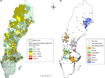
Fig. 1. (a) Mean tularemia incidence (cases/100 000 persons per year) per zip code areas during 1984–2012 and spatial distribution of tularemia cluster areas identified by SatScan using a 40-km maximum window radius size. (b) High-risk regions for tularemia in Sweden 1984–2012. Main municipalities and stations for meteorological and hydrological data are indicated.
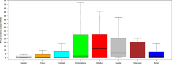
Fig. 2. Boxplots (without outliers) of the tularemia annual incidence in Sweden and the seven tularemia high-risk regions.
Table 1. Description of the seven identified high-risk tularemia regions (from south to north) of Sweden 1984–2012 with regards to population, number of tularemia cases, mean incidence during the study period, age, percent of male patients, and the peak season
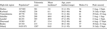
* Population census 2012.
† Cases/100 000 inhabitants/year.
‡ The seasonal period in which 50% of the cases occurred.
§ All region in Sweden not being classified as high-risk regions.
Variation in the number of tularemia cases
The variation of the annual number of tularemia cases (Tul) was prominent for all the high-risk regions with most of the larger outbreaks occurring in the later part of the study period (Fig. 3 and Supplementary Table S2). By pairwise comparisons, annual variations of Tul were found to be highly correlated between the high-risk regions (ρ = 0·33–0·85, Supplementary Table S3). High-risk regions located close to each other were more similar with regard to annual case variation than regions situated far from each other (Mantel's test, r = 0·63, P ⩽ 0·01). The majority of the tularemia disease onset dates occurred from the end of July to the beginning of September in all high-risk regions, although the season occurred a little later in Östersund (Fig. 4, Table 1). The annual median dates of disease onset were positively correlated for all pairs of regions and the correlation increased as the distance between the regions decreased (Mantel's test, r = 0·41, P ⩽ 0·05).
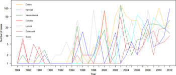
Fig. 3. The observed number of tularemia cases for the seven tularemia high-risk regions of Sweden 1984–2012.
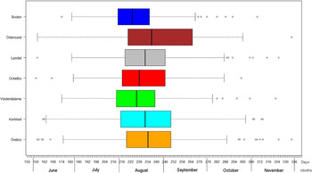
Fig. 4. Boxplots of reported dates of disease onset or diagnosis for the tularemia cases, reported between 1 June (day 154) and 30 November (day 336), in the seven tularemia high-risk regions of Sweden 1984–2012. Under each box, first quartile, median, and third quartile are reported.
Description of the predictor variables in the model
The annual variation of all predictors, except CW, were similar in the high-risk regions, with the highest pairwise correlations observed for STlag, followed by sRMA, and SP (Supplementary Tables 4–7). Regions located close to each other were more likely to display higher covariation than regions located far from each other (Mantel's test, sRMA: r = 0·68, P ⩽ 0·01; STlag: r = 0·55, P ⩽ 0·05; SP: r = 0·39, P > 0·05).
Covariation between the annual number of cases and the predictors
The dependent variable Tul was positively correlated with Tullag (ρ = 0·04–0·79) sRMA (ρ = 0·03–0·44), STlag (ρ = −0·09 to 0·36) and SP (ρ = 0·09–0·80); and negatively correlated with CW (ρ = −0·48 to 0·04) for all high-risk regions with two minor exceptions (Supplementary Table S8). There were no significant correlations between the different predictor variables (data not shown).
Modelling the annual variation of tularemia cases
The coefficients in the fitted models varied noticeably between the high-risk regions, but some trends were observed. The coefficients for the variables Tullag, sRMA, STlag, and SP were positive for all regions with three exceptions: the Tullag coefficient in Ockelbo, and the STlag and SP coefficients in Karlstad were all negative (Table 2).
Table 2. Estimated coefficients of the predictor variables in the fitted models explaining annual tularemia variation in the seven high-risk regions of Sweden (1984–2012)
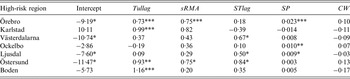
Predictors significantly different from zero are indicated: * P ⩽ 0·05, ** P ⩽ 0·01, *** P ⩽ 0·001.
The models were successful in modelling the annual variation of tularemia cases in most of the high-risk regions: a large fraction of the variation of Tul was explained (pseudo-R 2 = 0·33–0·76), the fitted and observed Tul values were highly correlated (ρ = 0·54–0·87), the estimated PPVs (reflecting the ability to estimate regional outbreaks) were high for most regions (PPV = 0·40–0·92), while the estimated NPVs were high for all regions (NPV = 0·79–1·00) (Table 3). Taking all performance measures into account, we concluded that the modelling was able to describe the annual variation of tularemia cases in the Southern regions, Örebro, Västerdalarna, Ljusdal, Ockelbo, and Karlstad, but was less successful in the most Northern regions Östersund and Boden (Table 3).
Table 3. Performance of the fitted models explaining annual tularemia variation in the seven high-risk regions of Sweden (1984–2012) with regard to pseudo-R2, Spearman's correlation between the fitted and observed annual number of tularemia cases (ρ), the positive predictive value (PPV), and the negative predictive value (NPV).
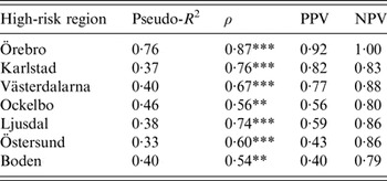
Correlations significantly different from zero are indicated: *P ⩽ 0·05, ** P ⩽ 0·01, *** P ⩽ 0·001.
DISCUSSION
We demonstrated that by using nationwide surveillance data, high-risk regions for contracting tularemia could be identified. The annual tularemia cases within these regions could be retrospectively modelled using easily accessible meteorological and hydrological data. The approach is broadly generalizable for defining high-risk regions, estimating predictors on a regional basis, and modelling the annual variation of tularemia cases. The results validated that modelling tularemia outbreaks is feasible in high-risk regions of Sweden and lays the foundation for developing an early warning system for outbreaks.
Historically, tularemia has repeatedly been described as a disease with uneven geographical distribution but the regions with increased risk of contracting tularemia have remained anecdotally defined. By taking the underlying population into account, we here developed a systematic and objective approach for identifying regions in Sweden where residents are at higher risk of acquiring tularemia. The results show that tularemia in Sweden is a highly geographically concentrated disease, with the majority of cases occurring within seven high-risk regions. We believe that our findings may help public health authorities to rationally assess the risk of tularemia in specific geographical locations and thereby provide more accurate information and early warnings to the public.
Large variation in tularemia incidence among the high-risk regions was identified, with the more densely populated regions generally having lower incidences. Importantly, there was also a very large local incidence variation within the high-risk regions. These findings were consistent with an ecological paradigm of tularemia being a geographically focal disease tied to disease vectors and hosts as was postulated already in the 1950s [Reference Pavlovsky17]. We here showed that the phenomenon of geographical focality readily translates into findings of large heterogeneity of disease risks at small spatial scales for humans. The results also support the many narratives of patients and physicians that the tularemia transmission is tied to specific localities. The identification of high-risk regions and geographical areas at smaller scales could help future studies to resolve unanswered questions with regard to tularemia ecology and local persistence by directing environmental sampling to these localities [Reference Johansson20–Reference Petersen and Molins22].
In previous work, the annual number of tularemia cases (Tul) in the Swedish county Dalarna which includes the high-risk region Västerdalarna identified in this study, was successfully modelled. We here generalized the modelling approach so that it could be used to model Tul in any region with sufficient number of cases. The approach utilized the tularemia case counts the previous year and local hydrological and meteorological data together with spatial interpolation to construct the regional predictor variables the standardized relative mosquito abundance (sRMA), the summer temperature (STlag), the summer precipitation (SP), and a proxy for hostile winter conditions for rodents, i.e. the number of cold days with little snow cover (CW) [Reference Rydén11].
We wanted to investigate if the variation of tularemia cases was similar in all the high-risk regions, if the predictors used in the model were relevant for all regions, and if the model could be used to model Tul within the high-risk regions. We found that Tul were highly correlated between the seven high-risk regions and that the pairwise correlations decreased as the distances between the regions increased. In addition, all high-risk regions had similar seasonal patterns with the majority of the cases occurring in July–September. This similarity suggests that the variation of Tul in different high-risk regions could be explained by the same predictors. It also suggests that the variation of Tul to a high degree was driven by the same variables in all the high-risk regions. All the predictors in the model behaved as if they were essentially independent and the predictors’ coefficients in the regional fitted models, except for the predictor CW, were overall positive. Altogether, these results suggest that a high number of cases the previous year, high relative mosquito abundance, high temperatures the preceding summer; and high summer precipitation are risk factors for regional tularemia outbreaks in Sweden.
The models’ negative predictive values were high for all high-risk regions meaning that non-outbreak years were successfully identified and although the positive predictive values were more variable, ranging between 0·40 and 0·92, the results imply that the models are capable of distinguishing between years with and without outbreaks. This capability would be practically valuable if it can be reproduced in future early-warning systems. A drawback of the present models was that they were fairly inaccurate in estimating the magnitude of the outbreaks, which resulted in relatively low pseudo-R 2 values. This was most evident for the two most Northern regions, Boden and Östersund. These results may indicate that the model was incomplete with one or several predictors missing, in particular for these Northern regions. Boden showed the lowest correlation between sRMA and Tul (data not shown) which may reflect that the regional prediction of sRMA was inadequate, that mosquitoes to lesser extent play a role for transmitting infection to humans, or that other routes of transmission have to be considered in this region (e.g. exposure to infected animals). The procedure for estimating the relative mosquito abundance using local hydrological and meteorological data was developed for an area in the middle part of Sweden, Dalarna, and it is unclear how this procedure performs in regions located far away. Correlation between sRMA and Tul was relatively high in Östersund (but not significant) while our model was inaccurate in this region, which may suggest that another epidemiological cycle of transmission, e.g. infection by inhalation of F. tularensis-contaminated dust, occurs in parallel with the common mosquito transmission cycle in this region [Reference Johansson20]. In a recent study from Finland it was shown that abundance of voles, which are believed to be the sources of infection in the inhalation-form of tularemia, highly correlated with tularemia incidence among humans but with a time-lag of one year [Reference Rossow23]. Unfortunately annual information on the regional vole abundance is currently not available for Sweden but an interesting future research direction is to include proxy variables for vole abundance to improve the current models.
We did not account for human behavioural factors in the modelling and this may be an important shortcoming because of variation in the exposure of humans to disease in different localities and due to their behaviour, e.g. time spent in outdoor activities. Regrettably, there was no data available validated to reflect exposure to tularemia. Future research should focus on improving the assessment of risk exposure by using data reflecting where people spend their time instead of using home addresses, for example data from questionnaires or GPS-enabled devices (e.g. mobile phones). Such data would define the population susceptible to tularemia better than census population.
We showed that a combination of surveillance and meteorological data including lag patterns of one year in the past can be used to predict summer tularemia outbreaks. However, the ability of the model to rapidly detect seasonal outbreaks is limited by the lack of some variables at the time of the prediction. Examples of data that will not be available without considerable lag are summer precipitation and river flow (used in the prediction of RMA) from June to August. At this stage of our research, the models cannot be used as an early warning tool but it surely constitutes a first step in the development of a reliable system to be used by public health authorities.
In conclusion, our study has identified where the high-risk regions for acquiring tularemia in Sweden are located. The results support a hypothesis of tularemia being tied to specific locations for long time periods, with the annual variation of cases driven by local ecological variables. In the coming years, increased knowledge of the ecology, dispersal, and persistence of tularemia will be needed for the identification of more precise predictors to further improve the modelling of annual variation of cases. Even though we here identified a useful model, testing of additional high quality data and making inference analyses using data in real-time will be required for developing a functional early-warning system for tularemia outbreaks.
SUPPLEMENTARY MATERIAL
For supplementary material accompanying this paper visit https://doi.org/10.1017/S0950268816002478.
ACKNOWLEDGEMENTS
The authors acknowledge the guidance and help given by Mattias Landfors, Rafael Björk, and Konrad Abramowicz. The authors also thank all physicians in Sweden and the epidemiologists at the Public Health Agency of Sweden who provided and curated the epidemiological information in the national communicable disease surveillance system, and the personnel at Statistics Sweden and at the Swedish Meteorological and Hydrological Institute for providing open data for research.
This work was supported by the Swedish Research Council for Environment, Agricultural Sciences and Spatial Planning (Formas no. 2012–1070) and Västerbotten County Council (Dnr. VLL-378261).
DECLARATION OF INTEREST
None.


