


INTRODUCTION
Influenza (flu or grippe) is among the most important epidemic diseases. Although preventable to a large extent, it still remains one of the most widely spread infectious diseases globally. Unfortunately, very often the timing, severity and exact strain of influenza remain uncertain. The spread of epidemics and pandemics of infectious diseases depends mainly on individual, physiological or immunological factors as well as on population/social and specific healthcare system phenomena but their appearance might also be related to various meteorological or heliogeophysical factors as part of the natural physical environment [Reference Chizhevsky1–Reference Hoyle and Wickramasinghe4]. The success of preventing influenza will depend largely on well-timed and precise forecasts about its incidence and, possibly, about the subtype of strains appearing by antigenic drift or shift [Reference Hoyle and Wickramasinghe4]. However, such forecasts in various geographical locations will be incomplete without considering the cyclic components of influenza incidence dynamics, its components and virulence patterns as well as the likely impact of physical environmental factors with similar cyclicity.
Previous studies of annual or monthly incidence and incidence rates across different countries have suggested the existence of high-frequency intrannual (<12 months), seasonal (annual) and low-frequency infrannual, trans-year or multiannual cycles. Trans-year cycles are those cycles with periods longer than 12 months, but shorter than 24 months. Various cyclic patterns have been observed, with periods of 1, 2–3, 5–6, 8·0, 10·6–11·3, 13 and 18–19 years; some of these have been associated with the influence of cyclic factors from the natural environment [Reference Chizhevsky1–Reference Ertel6]. Not all of the flu incidence time series have clearly defined linearly increasing or decreasing tendencies but, even so, they could not be easily forecasted ahead by linear trend analysis only. The latter is due to the presence of a high level of variability or volatility. It is possible that variations around such linear trends or mean values may show regular patterns and potentially be exploited in modelling and forecasting with derivation of future estimates and their 95% confidence intervals (CIs). Being of high public health and socioeconomic importance, the better forecasting of flu incidence variations and their peaks is invaluable for national health systems worldwide. Such forecast estimates may help in identifying populations at increased risk, highlighting the potential for immunization and allow a more adequate allocation of resources. This more precise forecasting will also allow an exploration of risk factors or triggers contributing to the appearance and spread of flu epidemics and pandemics.
Triggers for the increases and/or cyclic variations in flu incidence may be such factors of natural environmental origin as interrelated physico-chemical processes and irradiations of cosmic or terrestrial origin. They are known as ‘space weather’, i.e. solar, geomagnetic or cosmic ray activity whereas their dynamics show clear cyclic patterns with fluctuations at various frequencies, for instance from hours, days to months, years and tenths of years. Such natural physical activity influences may be also denoted by the common term ‘heliogeophysical activity’ (HGA). HGA mainly comprises phenomena such as solar activity and geomagnetic field fluctuations but it may also refer to a number of other photic or non-photic events. Such emitting events are sunspots, solar UV radiation, solar wind, 10·7-cm solar radio flux, neutron activity, earth-ionosphere cavity/Schumann resonances [Reference Cherry7] as indicated or described by quantitative indices such as the sunspot index, geomagnetic indexes (aa, Kp, Ap, Dst) or ozone concentration. Most of these indices exhibit seasonal or circa-annual cyclicity but their chronomes are often multicomponent, with trans-year or multiannual periods such as the 22-year cycle (Hale's solar magnetic cycle) or the 11-year cycle of the sunspot index (Rz index or Wolf number). The latter has been a consistent observation over hundreds of years [Reference Cherry7–Reference Komitov9]. Whether or not such cyclic patterns in flu incidence and HGA are interconnected, remains to be explored.
Previous approaches to flu incidence variations have mostly employed a visualization of cyclic variations [Reference Chizhevsky1, Reference Sidyakin2, Reference Hoyle and Wickramasinghe4], calculation of the number of peaks within pre-defined intervals of time [Reference Hope-Simpson3, Reference Hoyle and Wickramasinghe4] and/or indication of their parallelism to similar variations in cyclic environmental factors [Reference Chizhevsky1, Reference Sidyakin2]. However, other more accurate quantitative approaches in modelling and forecasting flu incidence are needed [Reference Dimitrov, Komitov and Dimitrova5, Reference Valev8–Reference Dimitrov, Atanassova and Rachkova10]. These methods, with minimal requirements for a specific algorithm and 95% CIs for the derived estimates and parameters [Reference Dimitrov, Atanassova and Rachkova10–Reference Dimitrov13] should be the following: (1) description, analysis and decomposition of temporal dynamics; nonlinear regression modelling of periodic mode; and derivation and forecasting of cyclic estimates; (2) linear and nonlinear regression modelling to independent variables (e.g. HGA) with such deterministic temporal patterns as seasonality. At present, the relationship of HGA cycles to flu incidence is of increasing importance in the view of the current maximum of the last 11-year solar cycle No. 24, as started in 2008 (http://www.kaltesonne.de/?p=13284).
Study objective
The aims of this study were: (i) to describe the temporal dynamics of monthly flu incidence in Azerbaijan for the years 1976–2000; (ii) to estimate any seasonal and multicomponent infrannual cycles and their eventual relationships with seasonality; and, (iii) to consider flu incidence cyclicity for similarities to and associations with main HGA cycles.
MATERIALS AND METHODS
Sources and description of time-series datasets
The time-series datasets consisted of monthly incidence data presented as an absolute number of new cases of influenza (ICD-9-CM, Dx: 487·0–487·8) in the Grand Baku area, Azerbaijan, (population >3 million). The incidence data were provided by the Azerbaijani State Institute of Advanced Studies of Doctors, Ministry of Health of the Republic of Azerbaijan. Average monthly and annual values of the international sunspot numbers (ISN) are freely available and were retrieved from the online database of the Solar Influences Data Analysis Center (SIDC) at the Royal Observatory of Belgium (http://sidc.oma.be/).
The flu incidence time series covered the period 1976–2000 (300 months, Fig. 1). The 25-year flu dataset, spanning over more than two 11-year cycles of solar activity (No. 21 and No. 22), was divided into three main intervals: interval 1 (1976–1990, n = 180 months), interval 2 (1991–1995, n = 60 months) and interval 3 (1996–2000, n = 60 months). This stratification was necessary to reflect the underlying demographic and socio-political changes that occurred during this period. The first interval was characterized by relative stability, with full medical care coverage (the so called ‘Soviet’ period, with obligatory healthcare); the second interval – by economic downturn due to the collapse of the USSR as characterized by difficulties and malfunctioning of the healthcare system; and the third interval – by further recovery and stabilization of the modern national healthcare system. All datasets are from public sources and can be obtained from the authors upon request.

Fig. 1 [colour online]. Dynamics of flu incidence in Grand Baku area, Azerbaijan and annual international sunspot numbers, 1976–2000.
Statistical analyses
Different statistical methods for time-series analyses and modelling were used (Table 1). Descriptive statistics with linear and nonlinear regression modelling over time were applied. As a second step, autocorrelation and spectral functions for amplitude and density were explored to examine whether the variations may exhibit cyclic patterns (Figs 2, 3). Last, a periodogram regression analysis (PRA) with determination of the cycle length and its statistical significance at P < 0·05 was applied [Reference Dimitrov, Komitov and Dimitrova5, Reference Dimitrov11–Reference Dimitrov14]. PRA, using the sigma method for testing the statistical significance of the linear correlation coefficients, was successfully applied in earlier studies on helioepidemiology of various cancers and infectious diseases [Reference Dimitrov, Komitov and Dimitrova5, Reference Dimitrov11–Reference Dimitrov13]. In this work we approximated the studied time series f(t) with a number of minimizing correlation-regression functions F(t) of periodic mode:
 $$F(t) = a_0 + A\cos \displaystyle{{2\pi t} \over T} + B\sin \displaystyle{{2\pi t} \over T},$
where a 0 is the mean of f(t) and T is a preliminary fixed, stepwise increasing period. The parameters A and B are coefficients of regression obtained by least-square calculations for the actual f(t) at each T; t is the current moment of time (a serial number of the month: 0, 1, 2, 3, …, N – 1), and N is the total number of values in the time-series sample [Reference Komitov9, Reference Dimitrov11, Reference Dimitrov15]. A range of the linear coefficients R is constructed against each of the tested periods T in months (Fig. 4) as a ‘periodogram’ of the time series, i.e. power in the period domain. The PRA with the use of basic, i.e. original, or detrended or decycled time series allows a description of the so-called ‘hypercycles’ on the periodogram. A ‘hypercycle’ is denoted when the length of its period T H exceeds the length of the analysed time-series set [Reference Dimitrov, Shangova-Grigoriadi and Grigoriadis16]. It is possible that such hypercycles represent or are closely related to the long-term linear or nonlinear trends, therefore the time series can be further decomposed. Then, the period/s T H can be removed later by decycling, a type of ‘detrending’ of the time series. The hypercycles may be also included in reconstructing and forecasting the incidence estimates by a trigonometric approximation when they are indicated to improve the forecasting power of the cyclic models [Reference Dimitrov13, Reference Dimitrov15]. SPSS 15 (SPSS Inc., USA), IBM SPSS Statistics 21 (IBM Corporation, USA) and a specialized package for time-series analyses ‘6D-STAT’ were used. The software ‘6D-STAT’ (www.astro.bas.bg/~komitov/dataproc.htm) was kindly provided by B. Komitov (Stara Zagora, Bulgaria).

Fig. 2 [colour online]. Autocorrelation analysis of flu incidence in Azerbaijan, 1976–2000. (a) Clear autocorrelation (r) peaks are seen where the lag number is in multiples of ≈12 months. (b) Partial autocorrelation function (r p) indicates that the strongest influence on monthly flu incidence was from the previous month (lag number = 1 month, r = 0·74) and ~1 year before (lag number peak at 11 months, r p = 0·25); a tendency of autocorrelation at 26 months may also exist (r = −0·13).
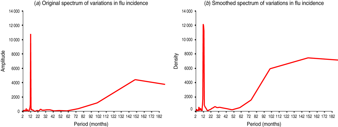
Fig. 3 [colour online]. Spectral analysis of flu incidence in Azerbaijan, 1976–2000. (a) The unsmoothed spectrum of amplitudes against the period indicated two main peaks at 12 and 152 months (spectral windows on a log scale of 10–18, 22–28 and 100–200 months, dara not shown). (b) The smoothed spectrum, where irregular variations have been removed, has confirmed the main peaks at similar periods of 12 and 150 months and a small, additional peak at 27 months (spectral windows on a log scale of 10–16, 22–30 and 50–200 months, data not shown). Of note, periods >150 months may represent artefacts or long-term trends in time series of 300 months where detrending/decycling was not applied a priori, therefore, such peaks should be viewed only as informative in nature and be interpreted with caution.

Fig. 4 [colour online]. Periodogram regression analysis (PRA) of cyclic patterns in the variations of flu incidence in Azerbaijan, 1976–2000. The periodograms show correlation coefficients R against period T (months). The peaks above the horizontal line indicate the significant periods at P < 0·05 (P = 0·05 for a theoretical R T = 0·11 at variance F≈2σ, n = 300) for original (red curve) and decycled/detrended (blue curve) time series. Y axis: correlation coefficient of R for flu incidence variations (the periods T = 12, 26 and 36 months are common for both time series in black font; periods T = 75 and 162 months are observed in the original in red font, while the period T = 113 months is secondary and it appears only in the decycled time-series, in blue font). (See Table 2 for more details.)
Table 1. Complex statistical approach to reveal and model cyclic patterns in incidence time series

RESULTS
Descriptive (exploratory) analyses
Descriptive analyses have shown that flu incidence in the Grand Baku area has remained mainly stable or slightly decreased during the study period from 1976 to 2000. However, the linear or nonlinear regression models by various functions [Reference Dimitrov13] have only been able to explain about 3–61% of the temporal variations. The best models were nonlinear, mainly of cubic, S-shaped or power/exponential type (data not shown). Notably, a minimum 39% of the variations remained unexplained even by decreasing tendencies. Such variations have indicated that analysing flu incidence by such trend models alone, even of nonlinear shape, will be of little use. We then postulated that the temporal distribution of flu incidence may be better represented by other nonlinear functions with high-frequency (seasonal, intrannual) and/or longer, low-frequency (trans-year, multiannual) cyclic components [Reference Dimitrov, Atanassova and Rachkova10, Reference Dimitrov13, Reference Dimitrov15].
Autocorrelation analysis
To provide evidence on the existence of cyclic variations, we constructed and analysed the autocorrelograms of flu incidence (Fig. 2). The autocorrelation function (ACF, Fig. 2 a) and partial autocorrelation function (Fig. 2 b) suggested that multiple cyclic components might co-exist with peaks in the windows of 1–22 and 64–92 as well as 132–156 months (data not shown). The main components of these windows are lag numbers, or cycles of 1 month showing dependence on the previous month, as well as for the previous 4 and 11 months (≈seasonal). Infrannual cycles of 82, 85 and 89 months were also detected (data not shown). Due to inherent limitations of the method where autocorrelations may only be evident when the low-frequency cycles are multiples of prevailing 12-month or other high-frequency components, to further confirm these patterns, a spectral analysis of flu incidence dynamics was also applied (Fig. 3).
Spectral analysis
To test above conjectures and better define the main existing cycles, we obtained spectral amplitudes and densities (Fig. 3). We described again the main 12-month cycle and provided further evidence on infrannual cycles of 27 months (2·3 years, Fig. 3 b), 102 months (8·5 years, Fig. 3 a) and, possibly, ≈150 months (12·5 years, Fig. 3 a,b). The latter may represent an artefact or a long-term trend in the flu incidence time series where detrending/decycling was not applied a priori. To further quantify and statistically confirm the above cyclic patterns, a periodogram analysis with correlation-regression function of periodic mode (see the Materials and Methods section for more details) was also applied (Fig. 4, Table 2).
Table 2. Cyclic patterns of variations in flu incidence time series in Grand Baku area, Azerbaijan (1976–2000)
* Statistical significance of the correlation coefficient R is denoted by p R after the z test at P < 0·05 when R > 1·96S R (z = R/S R), where S R is the standard error of R [Reference Komitov9]; R, correlation coefficient from the periodogram (i.e. PRA, periodogram regression analysis) indicating a peak at a particular period T of an underlying cyclic pattern (e.g. see periodograms in Fig. 4); p R, statistical significance of R; n, sample size of time series (months).
† Hypercycle (long-term cyclic pattern) is revealed when the period T H is longer than the sample size of the time series (see Dimitrov et al. [Reference Dimitrov, Shangova-Grigoriadi and Grigoriadis16] for further references on hypercyclicity).
Periodogram regression analysis
To better quantify and apply formal statistical confidence testing to the underlying cyclic patterns in flu incidence dynamics, we constructed periodograms (Fig. 4) and confirmed the main cycle of 12 months. This period appears to be the most important and repeated cyclic pattern across all stratifications. Beyond seasonality, several multiannual cycles with periods T in the ranges of 26–36, 62–85 and 113–162 months were also established, with an average period for T of 2·5, 6·1 and 11·5 years, respectively. For some of the intervals, one or more hypercycles were described. These may represent or be related to long-term nonlinear trends with periods T H = 128, 156, 194 and 208 months (i.e. hypercycles of 10·7, 13·0, 16·2 and 17·3 years, respectively; data not shown). PRA is now illustrated by depicting only the periodograms for the whole study period (1976–2000). All results for the different intervals and their combinations are summarized in Table 2.
Where an additional elaboration of the time series was considered appropriate in order to control for revealed cyclic patterns in the original time series, a decomposition and further decycling were applied. When removing the cycle of 162 months or a de-trending were applied, e.g. a new time series was derived and an additional periodogram was constructed again (e.g. see the blue curve in Fig. 4). It can be observed that after this procedure the three cycles with periods T = 12, 26 and 36 months remained significant. At the same time, while the cycles of 75 and 162 months disappeared, a new (secondary) cycle of 113 months appeared in the derived time series. Therefore, it can be suggested that the high-frequency cyclicity (annual and, possibly, short-term multiannual periods of 2–3 years) was not dependent upon the long-term nonlinear decreasing trend. Seasonality appears to be an independent, stand-alone stable cyclic pattern over the whole study period of 300 months. Of note, the main cyclic components of monthly flu incidence in Azerbaijan (1, 2–3, 6–7, 10–13, 16–17 years) may be considered similar to some of the most prominent cyclic components in such global HGA parameters as the sunspot index, F10.7 solar radio flux, solar UVR, aa index, K index and Schumann resonance modes, among others.
DISCUSSION
Descriptive, autocorrelation and regression analyses have shown clearly that cyclic patterns (beyond seasonality) may exist in the variations of time series of flu incidence in Azerbaijan over the years 1976–2000 (n = 300 months). First, we found that despite the extensive analysis and modelling, the usual linear or nonlinear models accounted only for up to 61% of overall variance. The remaining, minimum 39% variability was unaccounted for; moreover, the latter appeared most likely in cycles. Notably, the predominant cycles in flu incidence variations, beyond the seasonal one, are those having periods of 2–3, 6–7, 10–13 and 16–17 years. This is very interesting since a relatively recent study [Reference Dimitrov, Komitov and Dimitrova5] has shown that main cycles of 2·25–2·50 and 18–19 years exist in flu annual incidence rates (Bulgaria, 1941–1986, n = 46 years), thereby confirming earlier reports by Chizhevsky [Reference Chizhevsky1] and Sidyakin et al. [Reference Sidyakin2] on the existence of short-term multiannual cycles of 2–3 years in flu dynamics.
Some of the earlier studies on influenza incidence dynamics also postulated interesting patterns of cyclic appearance of flu incidence, with peaks at specific points along the 11-year solar activity cycle in the 20th century [Reference Chizhevsky1–Reference Hoyle and Wickramasinghe4]. Reports of flu pandemics, occurring around the sunspot maxima, were later scrutinized by Ertel [Reference Ertel6]. Ertel had reanalysed data on 25/42 ‘claimed’ pandemics during 1700–1985 (total n = 286 years) and suggested that their peaks tended to occur in years near the minima of these solar cycles but only during the 18th century. This relationship had probably declined over time thus becoming more complex during the 19th and 20th centuries, possibly showing unstable historical patterns. Another explanation might be, as suggested earlier by Chizhevsky [Reference Chizhevsky1], that flu incidence peaks (at least for 17th–19th centuries or earlier) appeared most likely on the ascending or descending slopes of the 11-year solar cycle. This means that the incidence peaks are most likely preceding and/or following the solar maxima by 1–2 years, probably influenced through the cyclic geomagnetic disturbances having double peaks, just before and after the peak of sunspot activity.
Sidyakin and colleagues [Reference Sidyakin2] also reported that flu death epidemic changes had been 1·3 times more frequent in the years of sudden increase in solar activity. They found that 42/44 flu death epidemics coincided with such intervals of sudden change. These authors also suggested that the cyclic variations of 2–4 years in flu epidemics could be associated with the frequency of such sudden changes, i.e. the so called ‘reference points’ along the 11-year sunspot cycle. Recent calculations indicated that such temporal appearances of flu epidemics [Reference Tapping, Mathias and Surkan17] were very likely when taking into account all cycles together since the year 1700 – Tapping and collaborators [Reference Tapping, Mathias and Surkan17] clearly illustrated by phase offset that five epidemic peaks occurred from ‘minimum’ to ‘minimum’ (inclusive) along the 11-year sunspot cycle.
Notably, we can assume that the main short-term multiannual (biennial/triennial) cycle in flu variation is the cycle with a period T = 2–3 years [Reference Dimitrov, Komitov and Dimitrova5], that is, beyond the prevailing seasonality and irrespective of the geographical location, i.e. similarly to malignant melanoma of the skin [Reference Dimitrov, Rachkova and Atanassova18]. Therefore, any other hierarchy of such cyclicity with a lower frequency of 6–7 years or 10–13 years may be considered [Reference Sidyakin2] as a ‘repetition’ of this principal, common period appearing along the curve of the 11-year sunspot cycle. Indeed, it is possible that for a given region flu incidence oscillates in several waves contemporaneously but in different phases. It is theoretically plausible that after a defined number of cycles or calendar years, the seasonally determined peak within the particular year may reach the highest possible level when all other close, shorter infrannual minor epidemic waves of 2–3 years or 5–6 years coincide. Such coincidences, or phase-locked temporal occurrences may certainly give rise to higher flu rates. These higher flu rates may express themselves with a major peak of a longer, infrannual flu cycle with a period T = 10–11 years [Reference Kilbourne19] or T = 18–19 years [Reference Dimitrov, Komitov and Dimitrova5]. Unfortunately, we are not able to further elucidate if such rises of major flu epidemics are due to one single flu strain causing the above-mentioned minor epidemics or if this is an appearance of new strains/variants (e.g. shift, drift), or a combination of both possible scenarios.
We cannot strongly conclude on the likelihood of HGA-related aetiological mechanisms of flu epidemic/pandemic peaks. However, if we consider about four minor epidemics during one average solar cycle, i.e. at the minimum, ascending slope, maximum and descending slope [Reference Tapping, Mathias and Surkan17], a role may be postulated for the solar UV radiation that clearly fluctuates along the 11-year cycle with high frequency [Reference Chizhevsky1, Reference Sidyakin2]. More recent publications have suggested a role for both UV radiation and vitamin D formation in the prevention of colds and flu [Reference Cannell20]. Therefore, minimum solar UV radiation, and possibly, a subsequent vitamin D decrease during the solar minima as well as at the solar maxima [Reference Chizhevsky1, Reference Sidyakin2] may easily facilitate the development and spread of influenza concomitantly, at about the same time intervals, but in different geographical locations. Being novel historically, at least in Britain as hypothesized still in 1940 [Reference Douglas21], and also more recently suggested for Azerbaijan [Reference Babayev, Maris and Messerotti22], these may be considered as very important conjectures. The temporal analyses and correlations between disease incidence and solar activity factors have been shown to be very useful in generating hypotheses and predictive models not only in influenza but also in other infectious diseases such as cholera [Reference Gumarova23]. It is of interet to quote here Dr Douglas Webster [Reference Douglas21], who wrote:
this and the often close correspondence between the monthly sun-spot oscillations and influenzal ‘waves’ (as, for instance, in the three pandemic waves of 1918–19) suggest the possible causal relationship of minor sun-spot cycles to cycles of virus activity in influenza.
To what extent such infrannual cyclicity of 2–3 years in flu incidence from the Grand Baku area in Azerbaijan is associated, or may interact with the underlying seasonality, as a main annual pattern is still largely unknown and may represent an interesting research question for further studies.
In conclusion, we summarize that by using a unique and relatively long time series of monthly data, we revealed a complex, multicomponent dynamics of flu incidence in Grand Baku area, Azerbaijan for the years 1976–2000. First, the main cyclic pattern was a seasonal period T = 12 months. Second, against the background of a long-term nonlinear decreasing trend, multiannual cyclicity with periods T = 26–36, 62–85 or 113–162 months was also described (average periods ≈2·5, 6·1 and 11·5 years, respectively). The cyclicity of 2–3 years was found to be the most interesting. Third, we established that most of these cycles correspond to similar HGA cycles and further analyses are warranted to investigate such relationships. Last, but not least, the specific cyclic patterns of flu incidence in Azerbaijan may not only advance our understanding of influenza aetiology, but may also contribute to the derivation of more precise forecasts for prevention and public healthcare purposes.
ACKNOWLEDGEMENTS
The authors thank Professor Dr F. E. Sadykhova, Azerbaijani State Institute of Advanced Studies of Doctors named after A. Aliyev, Ministry of Health, Republic of Azerbaijan, for providing the data on influenza and her helpful comments during the preparation of this manuscript. Special thanks are due also to Professor G. Cornelissen and the specialists from The Halberg Chronobiology Centre, University of Minnesota, USA, for their help and assistance provided during the revision of the manuscript. This study was initiated in 2009 when Dr Dimitrov was with the HRB Centre for Primary Care Research at the Royal College of Surgeons in Ireland.
DECLARATION OF INTEREST
None.


