


Impact Statement
Mutual style transformation between simulated and observed data was achieved using a neural network. This compensated for the lack of observational data in the construction of data-driven models with simulation data.
1. Introduction
In recent years, deep learning-based image recognition techniques have been applied to atmospheric science. Deep learning, a machine learning approach that utilizes neural networks with high representation capabilities through the connection of multiple layers of neurons, has demonstrated exceptional performance in recognizing atmospheric patterns. Numerous research reports have detailed the use of deep learning to detect extreme weather (Matsuoka et al., Reference Matsuoka, Sugimoto, Nakagawa, Kawahara, Araki, Onoue, Iiyama and Koyamada2019; Prabhat et al., Reference Prabhat, Kashinath, Mudigonda, Kim, Kapp-Schwoerer, Graubner, Karaismailoglu, von Kleist, Kurth, Greiner, Mahesh, Yang, Lewis, Chen, Lou, Chandran, Toms, Chapman, Dagon, Shields, Wehner and Collins2021), perform statistical downscaling (Harris et al., Reference Harris, ATT, Chantry, Dueben and Palmer2022), and parameterization (Rasp et al., Reference Rasp, Pritchard and Gentine2018). Several comprehensive review papers have also been published, encompassing diverse applications of these techniques to topics such as tropical cyclones (Chen et al., Reference Chen, Zhang and Wang2020), rainfall (Barrera-Animas et al., Reference Barrera-Animas, Oyedele, Bilal, Akinosho, JMD and Akanbi2022), and temperature forecasting (Tran et al., Reference Tran, Bateni, Ki and Vosoughifar2021). In particular, deep learning can be advantageous in situations where constructing models based on physical principles proves to be challenging. Moreover, the use of machine learning for improving observations and simulations is expected to increase in the future.
In general, the accuracy of machine learning-based pattern recognition decreases for phenomena with a small number of observed cases. In related research, a decline in recognition performance has been reported for tropical cyclone precursors in their early stages (Matsuoka et al., Reference Matsuoka, Nakano, Sugiyama and Uchida2018) and for super-large hurricanes (Pradhan et al., Reference Pradhan, Aygun, Maskey, Ramachandran and Cecil2018). This is a fundamental problem in supervised machine learning, which learns rules for pattern recognition from training data. Enhancing the predictive capabilities for cases with a limited amount of data has been one of the key challenges in machine learning.
One approach for avoiding the degradation of recognition accuracy is to artificially increase the amount of data with a small number of examples (Shorten & Khoshgoftaar, Reference Shorten and Khoshgoftaar2019). A method called “data augmentation” has been proposed to increase the amount of original data using geometric and color-space transformations. Particularly, data augmentation techniques, including vertical and horizontal flip, random crop, and random rotation, are widely recognized in image pattern recognition, and have been extensively employed in data analysis competitions for tropical cyclone detection (Matsuoka, Reference Matsuoka2021). In addition, attempts have been made to create new data using generative adversarial networks (GANs), a type of generative model (Goodfellow et al., Reference Goodfellow, Pouget-Abadie, Mirza, Xu, Warde-Farley, Ozair, Courville and Bengio2014). However, because the data created by GANs have very similar characteristics as the original data, it is uncertain whether data augmentation can improve recognition performance.
Numerical simulations can generate a large amount of data using multiple initial values and scenarios that are appropriate for use as training data in terms of data volume. Furthermore, simulation data typically contain a greater number of physical variables in comparison to observational data, and it is possible to generate labeled data with higher accuracy than humans by applying the tropical cyclone tracking algorithm to temperature, wind speed, and sea surface pressure data. Thus, simulation data can be used in conjunction with observational data. However, to use simulation and observational data simultaneously, it is necessary to match the two styles. Simulation data do not perfectly match the observed data in terms of patterns, owing to factors such as spatiotemporal resolution, physical schemes, and numerical noise. Therefore, it is not realistic to apply machine learning models learned from simulation data directly to observational data (Matsuoka, Reference Matsuoka2022).
In this study, cloud image data augmentation using style transformation techniques based on simulation data was used to reduce the degradation of the recognition accuracy caused by the lack of observational data. A style-transformation technique was used to transform the simulation data into the style of the observed data, and simultaneous learning with the observed data was achieved for model’s fine tuning. As a case study, the effectiveness of the method was verified by detecting tropical cyclone precursors during the early stages of their development.
2. Datasets
2.1. Observational data
We used infrared data (IR1) from GridSat-B1 as the satellite observational data for cloud distribution. GridSat-B1 data are provided by NOAA as a dataset that combines multiple satellite observations in the International Satellite Cloud Climatology Project on a grid of approximately 7 km for ease of use (Knapp & Wilkins, Reference Knapp and Wilkins2018). In this study, data from 1980 to 2017 in the Northwest Pacific were used.
For supervised machine learning, the above data were trimmed to an appropriate size and correctly labeled as tropical cyclones, their precursors (positive), or not (negative). To label positive cases, we used the best-track data of tropical cyclones obtained through IBTrACS version 4 published by NOAA’s National Climate Data Center. The best track data included the latitude and longitude of the center of the tropical cyclone, minimum pressure, and maximum wind speed. Additionally, it included information after the development of a tropical cyclone as well as information on tropical disturbances before they become tropical cyclones and after they changed to extratropical cyclones. In this study, a 128 $ \times $
128 grid (approximately 1,000 km2) rectangular area, including the center of the cyclone, was cut out as positive examples (TCs and preTCs). When the IR was normalized from 0 to 1 in the range of 200–300, the regions in the rectangular area with a mean value of 0.3 or higher that did not contain positive examples were cut out as negative examples (nonTCs). The total data comprised 39,115 positive and 977,812 negative examples.
$ \times $
128 grid (approximately 1,000 km2) rectangular area, including the center of the cyclone, was cut out as positive examples (TCs and preTCs). When the IR was normalized from 0 to 1 in the range of 200–300, the regions in the rectangular area with a mean value of 0.3 or higher that did not contain positive examples were cut out as negative examples (nonTCs). The total data comprised 39,115 positive and 977,812 negative examples.
Positive and negative examples taken from GridSat IR1 are shown in Figure 1a,b. The number of data points per elapsed time is shown in Figure 1d. The number of cases was highest at the moment of the onset of the tropical cyclone (zero elapsed time), and was smaller for preTCs with a longer time to onset. The number of cases 168 hr before the onset of the cyclone was 10 or less. Additionally, there were fewer cases 7–14 days prior to the outbreak.

Figure 1. Examples of (a) observed TCs and preTCs, (b) observed nonTCs, and (c) simulated TCs and preTCs. The numbers of training and/or test data of (d) observation and (e) simulation in each elapsed time.
2.2. Simulation data
In this study, we used 30-year climate simulation data produced by the nonhydrostatic icosahedral atmospheric model (NICAM) with a 14-km horizontal resolution (Kodama et al., Reference Kodama, Yamada, Noda, Kikuchi, Kajikawa, Nasuno, Tomita, Yamaura, Takahashi, Hara, Kawatani, Satoh and Sugi2015). Fully compressible nonhydrostatic equations guarantee the conservation of mass and energy. This study is not specific to any particular model; for more information on the NICAM, see the survey by Satoh et al. (Reference Satoh, Tomita, Yashiro, Miura, Kodama, Seiki, Noda, Yamada, Goto, Sawada, Miyoshi, Niwa, Hara, Ohno, Iga, Arakawa, Inoue and Kubokawa2014).
Similar to the observational data, the training data for machine learning were prepared as simulation data. A tropical cyclone tracking algorithm (Sugi et al., Reference Sugi, Noda and Sato2002; Nakano et al., Reference Nakano, Sawada, Nasuno and Satoh2015; Yamada et al., Reference Yamada, Satoh, Sugi, Kodama, Noda, Nakano and Nasuno2017) was applied to the 30-year NICAM data, and 754 TC tracks in the western North Pacific were extracted. The algorithm uses sea-level pressure, temperature, and wind field data to detect tropical cyclones and was optimized for NICAM data. From the extracted tracks, the outgoing longwave radiation (OLR) data of a 64 $ \times $
64 grid (approximately 1,000 km2) rectangular area, including the center of the tropical cyclone, were cut out as the training data. The number of examples extracted in this way was 35,060 (13,514 preTCs and 21,546 TCs). Because the NICAM data were used only for style conversion of positive examples (TC and preTC), negative examples (nonTC) were not included.
$ \times $
64 grid (approximately 1,000 km2) rectangular area, including the center of the tropical cyclone, were cut out as the training data. The number of examples extracted in this way was 35,060 (13,514 preTCs and 21,546 TCs). Because the NICAM data were used only for style conversion of positive examples (TC and preTC), negative examples (nonTC) were not included.
Some positive examples of the NICAM data are presented in Figure 1c. Compared with the positive examples of GridSat IR, qualitatively, the images appear blurred with a less fine structure. The amount of data per unit of elapsed time is shown in Figure 1e. The observational data show only 10 cases 168 hr before the event, whereas the simulation data show more than 200 cases.
3. Method
3.1. Method overview
The framework of the proposed method consists of two types of convolutional neural networks (CNNs): neural style transfer and binary classification. An overview of the proposed method is presented in Figure 2. Neural style transfer involved training to transform the features of the observational and simulation data. This framework was used to convert the simulation data (only a positive example) into an observation-like style. The binary classification involved two steps. In the first step, only observational data are input into the CNN and the binary classifier was trained. In the second step, additional training of the binary classifier was performed by inputting the observational data and observation-like data converted from the simulation data by neural style transfer. The trained classifier was then applied to the observational data not used for training to evaluate the detection performance. In the following sections, we describe the architecture of each CNN and its experimental settings.

Figure 2. Schematic diagram in the training phase of the proposed method.
3.2. Style transfer between simulation and observational data
We transformed the simulation data into observation-like data using CycleGAN (Zhu et al., Reference Zhu, Park, Isola and Efros2017), which is a method for mutually transforming data in two different domains. Because the NICAM data do not reproduce the actual atmosphere by data assimilation, they do not perfectly match the GridSat cloud distribution. Therefore, CycleGAN is a promising approach because it enables conversion using unpaired data, unlike conversion methods that use paired data, such as pix2pix (Isola et al., Reference Isola, Zhu, Zhou and Efros2017). CycleGAN trains using unpaired data for function F, which transforms from domain X to domain Y, and function G, which transforms from domain Y to domain X. We used adversarial loss to learn a mapping G that produced a distribution G(X) that was indistinguishable from the target distribution Y. In this study, because the adversarial loss alone was not binding, we introduced a cycle consistency loss to correct F(G(X)) so that it could recover X. The same process was used to train the transformation in the reverse direction. We used 4,000 training data each for both simulated and observed data (1999–2004), and repeated the training for 3,800 epochs until the error (sum of adversarial loss and cycle consistency loss) converged. The error (RMSE) between x sim and G(F(x sim)) was 5.9–17.1 W/m2 (12.2 W/m2 on average) and between x obs and F(G(x obs)) was 3.8–5.8 K (4.9 K on average) for the test data (2005–2008) for the trained CycleGAN. Here, x sim and x obs are simulation and observational data, respectively. F and G are the mapping function from the simulation data to the observational data and from the observational data to the simulation data, respectively.
3.3. Binary classification
A binary classification model was constructed for GridSat IR data to distinguish between TCs and nonTCs. The details of the classification model are beyond the scope of this study; however, we used the ResNet-18 model (He et al., Reference He, Zhang, Ren and Sun2016), a deep CNN with 18 layers. ResNet is an architecture that efficiently propagates gradients from the output layer to the input layer by introducing a Residual Module that skips between multiple layers. The input data are a single channel of data corresponding to the cloud distribution, and the output classes are TCs/preTCs (positive) and nonTCs (negative).
To evaluate the effectiveness of the proposed method, four classification models were constructed using different training data settings (Table 1). Model 1 was a baseline classifier model constructed by training only the observational data. Model 2 was not a realistic configuration, but a model that trained only simulation data to be used as a reference for comparison. Models 3 and 4 performed fine-tuning by learning additional simulation data as positive examples for Model 1. Model 4 trained the transformed simulation data in addition to the observational data using CycleGAN, whereas Model 3 trained the simulation data directly. In the first and second stages, training was repeated until the error between the predicted and correct classes converged. The error function was defined by the binary cross entropy. In all models, the validation data were 10% of the training data, and the test data for evaluation were the observational data not used for training. The test data were unbalanced, with a 50-fold difference in balance: 958,845 negative examples compared to 20,148 positive examples. As seen in previous studies (Matsuoka et al., Reference Matsuoka, Nakano, Sugiyama and Uchida2018; Matsuoka, Reference Matsuoka2021; Matsuoka, Reference Matsuoka2022), the training dataset shows an artificially balanced class distribution for efficient learning, whereas the test dataset shows class imbalances similar to real applications.
Table 1. Training data setting for each classification model. The numbers of positive examples (P) and negative examples (N)

4. Results and discussion
4.1. Style transformation
Using a style transformation, the OLR of the simulated data was converted into the IR of the observed data. Figure 3 shows the examples of the original simulation images and the results of the transformation into the observed style. Qualitatively, the cloud structure of the simulation data was converted into a fine scale. In this figure, a color map wherein the cumulative distribution functions before and after the transformation are nearly identical is provided. The results showed no significant alterations in the cloud form, only an improvement in the resolution of their texture.

Figure 3. Results of neural style transfer from (a) simulated clouds to (b) observed-like clouds.
Style transformation improved the frequency distribution of the physical quantities representing clouds in the simulation. Figure 4a–c shows the differences in the cloud histograms before and after the style transformation. The simulated tropical cyclone had a flat cloud-top and was dominated by high clouds (lower OLR value in Figure 4b). However, the distribution representing the cloud-tops of the tropical cyclones after the transformation (lower value of IR in Figure 4c) was not flat and was in good agreement with the distribution of the observational data (Figure 4a). The distribution of low clouds was also in good agreement before and after the conversion. Similarly, the histogram of the horizontal gradient of clouds shows an improvement owing to the style transformation, as shown in Figure 4d–f. In particular, the distribution of horizontal gradients near zero indicates that the weak horizontal gradients of clouds reproduced by the simulation were improved by the style transformation.
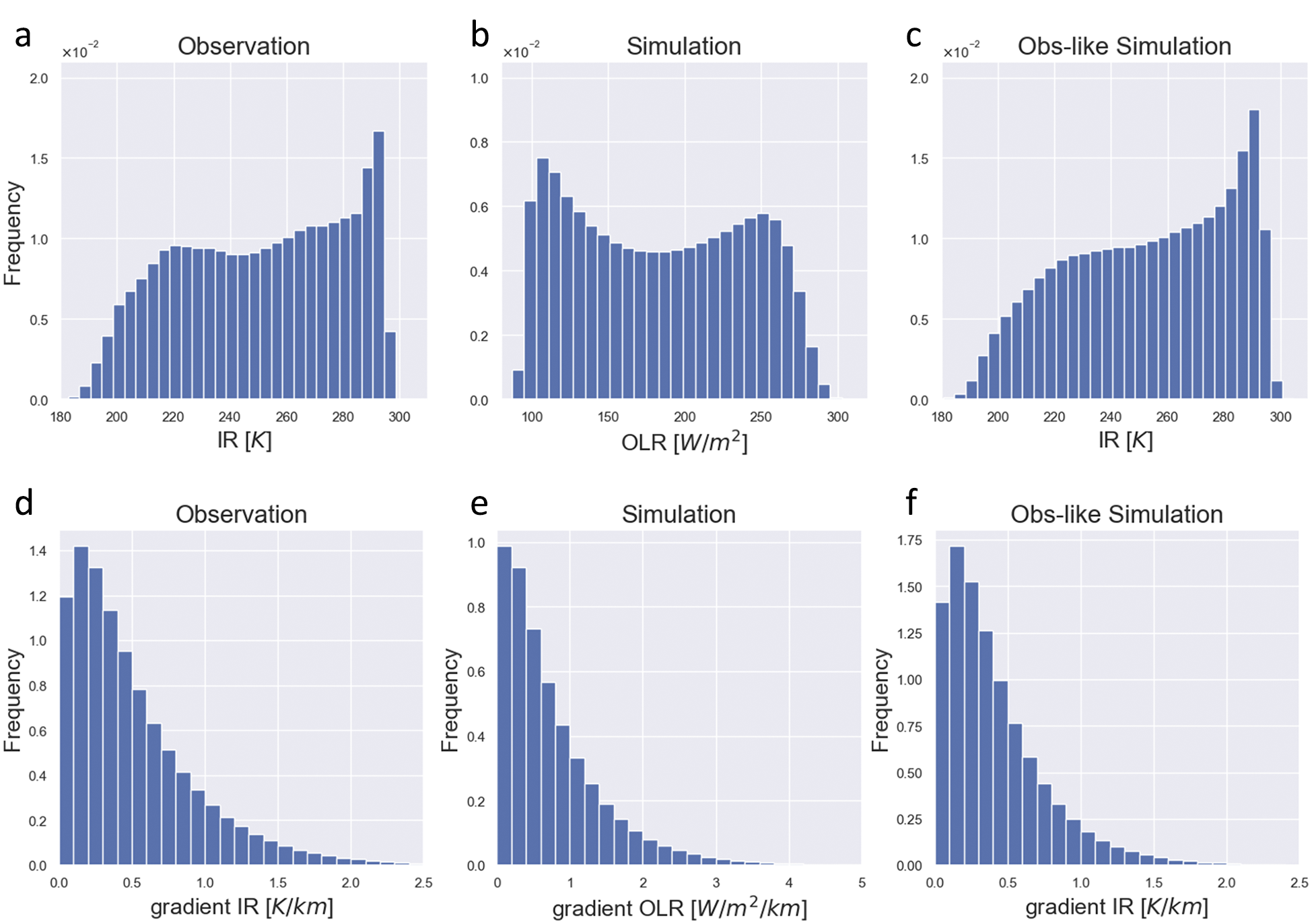
Figure 4. Histograms of clouds (a) observation, (b) simulation, and (c) observation-like data. Histograms of spatial gradient of clouds (d) observation, (e) simulation, and (f) observation-like data.
4.2. Classification performance
Additional training using the style-transformed simulation data improved the classification performance for the test data (observational data) compared with training using only the observational data. Figure 5a shows the classification performance of the four models as precision–recall curves (P–R curves). The larger the area between the P–R curve and the vertical and horizontal axes (area under the curve [AUC]), the higher the accuracy. The model with the highest classification accuracy was the model trained on transformed simulation data (Model 4), with an AUC of 0.95, compared with 0.91 for Model 1, the model trained on observational data alone. For reference, the AUCs for Models 2 and 3 are 0.83 and 0.91, respectively.

Figure 5. Classification performance of four models for test observational data. (a) Precision–recall curves and (b–d) recall with 95% confidence interval for each elapsed time when precisions are fixed at 0.5, 0.7, and 0.9, respectively. Note that in (a), the PR curve of Model 1 almost overlaps that of Model 3.
Additionally, the detection accuracy for tropical cyclone precursors in the early stages of their development improved. Figure 5(b–d) shows the recall for each elapsed time when the precision was fixed at 0.5, 0.7, and 0.9, respectively. The recall of Model 4 was the highest from 7 days prior to the onset of the tropical cyclone to the time of the onset of the cyclone. In particular, in the case of precision = 0.9, the recall at 7, 5, and 3 days before the TC formation improved by 40.5, 90.3, and 41.3%, respectively, compared with the model trained only with observational data. The model trained only on the simulation data (Model 2) exhibited the lowest classification accuracy. Similarly, the model trained directly on the simulation data (Model 3) did not show a significant improvement in accuracy. As seen in previous studies (Matsuoka et al., Reference Matsuoka, Nakano, Sugiyama and Uchida2018), the detection skill of TCs in the early stages is decreased because there is less training example and the shape is not well formed (e.g., 7–14 days before the TC formation). Furthermore, it should be noted that the range of confidence intervals for detection skill is larger during these periods due to the lack of test data.
5. Conclusion
In this study, we propose an approach to compensate for the lack of observed cases using simulation data in supervised machine learning to improve the detection accuracy of tropical cyclone precursors. The simulation data were converted to a style similar to that of observational data by learning-style conversion between the simulated and satellite-observed cloud images. The simulated data with style transformation were confirmed to have a frequency distribution similar to that of the observed data. Incorporating these data in the training improved the detection accuracy of tropical cyclone precursors up to 7 days before onset by 41.2% on average. This represents a novel application of simulations in the machine learning era.
Although this study only dealt with clouds, similar style transformations may be applied to other scalar and vector quantities. In atmospheric sciences, studies have reported the utilization of transfer learning through the use of simulation and reanalysis data, with the aim of precipitation measurement (Sambath et al., Reference Sambath, Viltard, Barthès, Martini and Mallet2022), precipitation forecast (Gibson et al., Reference Gibson, Chapman, Altinok, Monache, MJ and Waliser2021), and so forth. It is anticipated that these methods will emerge as a pioneering approach to utilize numerical models. As mentioned earlier, simulations cannot perfectly reproduce real atmospheric conditions because of limitations in factors such as spatiotemporal resolution and physical schemes. However, learning and understanding the process of converting simulated data to observed data can enable the quantification of the characteristics of the simulation model, thus leading to its advancement in the future.
Abbreviations
- CNN
-
convolutional neural network
- GAN
-
generative adversarial network
- GridSat
-
gridded satellite
- IR
-
infrared
- NICAM
-
nonhydrostatic icosahedral atmospheric model
- OLR
-
outgoing longwave radiation
Acknowledgments
We are grateful to Drs. M. Nakano, C. Kodama, and Y. Yamada for providing the training and test data on tropical cyclones. We would also like to thank Drs. S. Mouatadid and W. Yu for meaningful discussions.
Author contribution
Conceptualization: Both authors; Data curation: D.M.; Data visualization: D.M.; Methodology: Both authors; Writing—original draft: D.M. Both authors approved the final submitted draft.
Competing interest
The authors have no competing interest.
Data availability statement
The NICAM simulation data are available in Mendeley Data (https://data.mendeley.com/datasets/xtvvkfvycr/1). The GridSat observational data are available in their website (https://www.ncei.noaa.gov/products/gridded-geostationary-brightness-temperature). Please contact the corresponding author for other data and source code request.
Ethical standard
The study met all ethical guidelines and adhered to the legal requirements of the study country.
Funding statement
This research was supported by grants from the JST, PRESTO (Grant No. JPMJPR1777), JST, CREST (Grant No. JPMJCR1663), JSPS KAKENHI (Grant No. JP22H01316), and CCAI (Grant No. 150).
Provenance
This article is part of the Climate Informatics 2023 proceedings and was accepted in Environmental Data Science on the basis of the Climate Informatics peer-review process.


 Open access