


Impact Statement
Bayesian modeling provides a fruitful ground for the nuanced combination of multiple climate model outputs when predicting the Earth’s climate characteristics for the coming years. We outline one such model and describe an empirical Bayes estimation approach that is computationally efficient. The proposed methodology, when applied to CMIP6 global temperature datasets, demonstrates that using empirical Bayesian techniques is better than using the simple “model democracy” approach of assigning equal weight to each climate model. We also obtain uncertainty bounds for the global temperature prediction problem.
1. Introduction
This paper is on predictive climate modeling using outputs of multiple models. The topic of how to assign weights to different climate models has been debated at length in the atmospheric science community. One approach is to assign equal weight to each model (Knutti, Reference Knutti2010). A more tailored approach is taken in Braverman et al. (Reference Braverman, Chatterjee, Heyman and Cressie2017) and Chatterjee (Reference Chatterjee2019), where models are assigned scores based on their performance in capturing probabilistic properties of observed climate data. Bayesian approaches with uncertainty quantification may be found in Tebaldi et al. (Reference Tebaldi, Smith, Nychka and Mearns2005) and Smith et al. (Reference Smith, Tebaldi, Nychka and Mearns2009). Other approaches for using information from multiple climate models may be found in Flato et al. (Reference Flato, Marotzke, Abiodun, Braconnot, Chou, Collins, Cox, Driouech, Emori and Eyring2014), Craigmile et al. (Reference Craigmile, Guttorp and Berrocal2017), Knutti et al. (Reference Knutti, Sedlacek, Sanderson, Lorenz, Fischer and Eyring2017), Sanderson et al. (Reference Sanderson, Wehner and Knutti2017), and Abramowitz et al. (Reference Abramowitz, Herger, Gutmann, Hammerling, Knutti, Leduc, Lorenz, Pincus and Schmidt2019). In essence, most techniques directly or implicitly balance the performance of any candidate model output on how closely it emulates current and historical data, and on how well it imitates the outputs of other climate models.
A fundamental scientific reason for studying multimodel ensembles is that the same physical processes and forces are used for all reasonable climate models, and these processes also govern the observed climate data (Masson and Knutti, Reference Masson and Knutti2011). In this paper, we leverage this property of a shared physical basis for all climate model outputs and observed data concerning global temperature data. First, we adopt a statistical framework that assumes that the climate models’ output and real data all share a common trend function over time. Second, we assume that the various model outputs and observed data are dependent on each other. This dependency is captured by framing the  $ L $ climate model outputs and the observed data as an
  $ L+1 $-dimensional random vector at any point in time. This allows the entire dataset in
  $ L+1 $-dimensions over time to be viewed as a vector Gaussian process, which we discuss in some detail in Section 2.2. However, this leads to extremely challenging computations as well as a lack of transparency in the intermediate steps, hence we use an empirical Bayesian (EB) approach in this paper.
We analyze the climate model outputs associated with the Coupled Model Intercomparison Project, now in its sixth phase (CMIP6), which directs research in fundamental areas of climate science (Eyring et al., Reference Eyring, Bony, Meehl, Senior, Stevens, Stouffer and Taylor2016). It organizes the federated efforts of many investigators whose model simulations examine natural climate variability and sensitivity. CMIP6 simulations occur under a wide range of scenarios characterized by a shared socioeconomic pathway (SSP) and a level of increased radiative forcing. The SSPs describe a spectrum of possible futures in terms of human energy use, population, and sentiment toward climate stewardship (Riahi et al., Reference Riahi, Van Vuuren, Kriegler, Edmonds, O’neill, Fujimori, Bauer, Calvin, Dellink and Fricko2017). They then inform the quantification of land use, energy consumption, and other factors used by climate modelers. Radiative forcing concerns the increase in energy transferred through Earth’s atmosphere, relative preindustrial levels (Intergovernmental Panel On Climate Change, 2007). We analyze model output under SSP-5 with a radiative forcing value of 8.5 watts/m $ {}^2 $, the most aggressive increase. The SSP-5 narrative describes an increase in economic capital driven by fossil fuel extraction and an overall technology-driven strategy to climate change mitigation.
The focus of our analysis is the output from a selection of 17 CMIP6 simulations (Bentsen et al., Reference Bentsen, Olivie, Seland, Toniazzo, Gjermundsen, Graff, Debernard, Gupta, He, Kirkevag, Schwinger, Tjiputra, Aas, Bethke, Fan, Griesfeller, Grini, Guo, Ilicak, Karset, Landgren, Liakka, Moseid, Nummelin, Spensberger, Tang, Zhang, Heinze, Iversen and Schulz2019; Dix et al., Reference Dix, Bi, Dobrohotoff, Fiedler, Harman, Law, Mackallah, Marsland, O’Farrell, Rashid, Srbinovsky, Sullivan, Trenham, Vohralik, Watterson, Williams, Woodhouse, Bodman, Dias, Domingues, Hannah, Heerdegen, Savita, Wales, Allen, Druken, Evans, Richards, Ridzwan, Roberts, Smillie, Snow, Ward and Yang2019; Good et al., Reference Good, Sellar, Tang, Rumbold, Ellis, Kelley and Kuhlbrodt2019; Lijuan, Reference Lijuan2019; Rong, Reference Rong2019; Schupfner et al., Reference Schupfner, Wieners, Wachsmann, Steger, Bittner, Jungclaus, Fruh, Pankatz, Giorgetta, Reick, Legutke, Esch, Gayler, Haak, de Vrese, Raddatz, Mauritsen, von Storch, Behrens, Brovkin, Claussen, Crueger, Fast, Fiedler, Hagemann, Hohenegger, Jahns, Kloster, Kinne, Lasslop, Kornblueh, Marotzke, Matei, Meraner, Mikolajewicz, Modali, Muller, Nabel, Notz, Peters-von Gehlen, Pincus, Pohlmann, Pongratz, Rast, Schmidt, Schnur, Schulzweida, Six, Stevens, Voigt and Roeckner2019; Seland et al., Reference Seland, Bentsen, Olivie, Toniazzo, Gjermundsen, Graff, Debernard, Gupta, He, Kirkevag, Schwinger, Tjiputra, Aas, Bethke, Fan, Griesfeller, Grini, Guo, Ilicak, Karset, Landgren, Liakka, Moseid, Nummelin, Spensberger, Tang, Zhang, Heinze, Iversen and Schulz2019; Semmler et al., Reference Semmler, Danilov, Rackow, Sidorenko, Barbi, Hegewald, Pradhan, Sein, Wang and Jung2019; Shiogama et al., Reference Shiogama, Abe and Tatebe2019; Swart et al., Reference Swart, Cole, Kharin, Lazare, Scinocca, Gillett, Anstey, Arora, Christian, Jiao, Lee, Majaess, Saenko, Seiler, Seinen, Shao, Solheim, von Salzen, Yang, Winter and Sigmond2019a,Reference Swart, Cole, Kharin, Lazare, Scinocca, Gillett, Anstey, Arora, Christian, Jiao, Lee, Majaess, Saenko, Seiler, Seinen, Shao, Solheim, von Salzen, Yang, Winter and Sigmondb; Tachiiri et al., Reference Tachiiri, Abe, Hajima, Arakawa, Suzuki, Komuro, Ogochi, Watanabe, Yamamoto, Tatebe, Noguchi, Ohgaito, Ito, Yamazaki, Ito, Takata, Watanabe and Kawamiya2019; Wieners et al., Reference Wieners, Giorgetta, Jungclaus, Reick, Esch, Bittner, Gayler, Haak, de Vrese, Raddatz, Mauritsen, von Storch, Behrens, Brovkin, Claussen, Crueger, Fast, Fiedler, Hagemann, Hohenegger, Jahns, Kloster, Kinne, Lasslop, Kornblueh, Marotzke, Matei, Meraner, Mikolajewicz, Modali, Muller, Nabel, Notz, Peters-von Gehlen, Pincus, Pohlmann, Pongratz, Rast, Schmidt, Schnur, Schulzweida, Six, Stevens, Voigt and Roeckner2019; Xin et al., Reference Xin, Wu, Shi, Zhang, Li, Chu, Liu, Yan, Ma and Wei2019; Yukimoto et al., Reference Yukimoto, Koshiro, Kawai, Oshima, Yoshida, Urakawa, Tsujino, Deushi, Tanaka, Hosaka, Yoshimura, Shindo, Mizuta, Ishii, Obata and Adachi2019; Ziehn et al., Reference Ziehn, Chamberlain, Lenton, Law, Bodman, Dix, Wang, Dobrohotoff, Srbinovsky, Stevens, Vohralik, Mackallah, Sullivan, O’Farrell and Druken2019; NASA Goddard Institute for Space Studies (NASA/GISS), 2020). All simulations were conducted under the SSP-5 8.5 scenario and produced monthly mean global near-surface air temperature values spanning 1850 January to 2100 December. We remove seasonality by subtracting the mean global monthly values from 1961 to 1990 (Jones et al., Reference Jones, New, Parker, Martin and Rigor1999). Constructing anomaly data and deseasonalizing it with a baseline of the averages over a 30-year time window is standard in climate data science. A 30-year period is often considered long enough for averaging out high-frequency weather-related variations, and the data between 1960 and 1990 is considered reliable, having adequate global coverage and modern enough for use as a baseline (Jones et al., Reference Jones, Horton, Folland, Hulme, Parker and Basnett1999; Shaowu et al., Reference Shaowu, Jinhong and Jingning2004; Valev, Reference Valev2006). With these, we forecast the observed monthly mean global near-surface air temperature, which is available from 1850 January to 2020 December (Morice et al., Reference Morice, Kennedy, Rayner, Winn, Hogan, Killick, Dunn, Osborn, Jones and Simpson2021). In all cases, we employed a simple (unweighted) mean and did not perform any regridding of the data beforehand.
2. Methods
2.1. Hierarchical Bayesian model
The 17 CMIP6 simulations produce monthly global near-surface air temperatures from 1850 to 2100. Let  $ {Y}_{\mathrm{\ell},t} $ be the deseasonalized, mean-centered time series from
  $ \mathrm{\ell} $th CMIP6 climate simulation for
  $ \mathrm{\ell}\hskip0.35em =\hskip0.35em 1,\dots, L\hskip0.35em =\hskip0.35em 17 $ and month
  $ t\hskip0.35em =\hskip0.35em 1,\dots, T\hskip0.35em =\hskip0.35em 3,012 $, where
  $ t\hskip0.35em =\hskip0.35em 1 $ corresponds to 1850 January. The observed monthly values through 2020 are denoted by
  $ {Y}_{0,t} $. The vector
  $ {\boldsymbol{Y}}_t $ will represent all values at month
  $ t $, and
  $ {\boldsymbol{Y}}_{\mathrm{CMIP},t} $ will represent the
  $ L $ climate simulations, that is,
 $$ {\boldsymbol{Y}}_t\hskip0.35em =\hskip0.35em \left[\begin{array}{c}{Y}_{0,t}\\ {}{Y}_{1,t}\\ {}\vdots \\ {}{Y}_{L,t}\end{array}\right];\hskip1em {\boldsymbol{Y}}_{\mathrm{CMIP},t}\hskip0.35em =\hskip0.35em \left[\begin{array}{c}{Y}_{1,t}\\ {}\vdots \\ {}{Y}_{L,t}\end{array}\right]. $$
 There are many ways to utilize these values when making predictions for  $ {Y}_{0,t} $. A simple method is to estimate a common mean function
  $ \mu (t) $ shared by all the climate simulations and observed data. Here, our goal is to also leverage the information contained within the plurality of these simulations beyond their mean. One such method is to assume
 $$ {\boldsymbol{Y}}_t\mid {\boldsymbol{U}}_t\hskip0.35em =\hskip0.35em \mu (t){\mathbf{1}}_{L+1}+{\boldsymbol{U}}_t,\hskip1em \mathrm{where}\hskip0.5em {\boldsymbol{U}}_t\overset{\mathrm{i}.\mathrm{i}.\mathrm{d}.}{\sim }{N}_{L+1}\left(\mathbf{0},\Sigma \right), $$
where  $ {\mathbf{1}}_{L+1} $ is an
  $ L+1 $-dimensional vector of 1’s, and
  $ {\boldsymbol{U}}_t $ are independent random effects. These random elements are independent over time but dependent between the
  $ L+1 $ time series. Our assumption here is that these are normally distributed, but this can be relaxed.
One may wonder if assuming the  $ {\boldsymbol{U}}_t $ are independent over time, or identically distributed, is adequate for the available climate data. However, our extensive preliminary studies strongly indicate that there is no temporal dependency pattern in the
  $ {\boldsymbol{U}}_t $: we have experimented using autoregressive integrated moving average (ARIMA) models, several kinds of Gaussian process-based models, conditionally heteroscedastic models, and change-point detection procedures. All these preliminary studies indicate that (2) is the best option for modeling
  $ {\boldsymbol{U}}_t $. However, note that our main modeling principle and ideas do not depend on the particular assumptions surrounding (2). We can easily replace the Gaussian distributional assumption or the independence assumption with other suitable conditions; however, in such cases, even the EB computations would be considerably lengthier and numerical integration-driven.
We represent the common monthly mean  $ \mu (t) $ with a Gaussian process defined by the covariance kernel
  $ {k}_{\alpha}\left(\cdot, \cdot \right) $ parameterized by
  $ \alpha $. The choice of kernel defines the class of functions over which we place our Gaussian process prior; here we have opted to use the squared exponential kernel. Since we have deseasoned our data, we may forgo explicitly encoding seasonality in the kernel (as in, e.g., Williams and Rasmussen, Reference Williams and Rasmussen2006, section 5.4). We also wanted to avoid placing any strict shape restrictions, for example, linear or polynomial. Finally, the Matérn
  $ 5/2 $ kernel is a common alternative to the squared exponential, but our experimentation did not find a meaningful difference between the two. Please see Section 3 of the Supplementary Material for more details. The squared exponential kernel is parameterized by
  $ \alpha \hskip0.35em =\hskip0.35em \left({\sigma}^2,\gamma \right) $, the variance and lengthscale parameters. That is,
 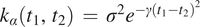 $ {k}_{\alpha}\left({t}_1,{t}_2\right)\hskip0.35em =\hskip0.35em {\sigma}^2{e}^{-\gamma {\left({t}_1-{t}_2\right)}^2} $. This and equation (2) define the hierarchical model given below:
 $$ {\displaystyle \begin{array}{l}{\boldsymbol{Y}}_t\hskip0.35em \mid \hskip0.35em \mu (t),\hskip0.35em \Sigma \hskip0.35em \sim \hskip0.35em {N}_{L+1}\left(\mu (t){\mathbf{1}}_{L+1},\Sigma \right),\\ {}\hskip4.4em \mu (t)\hskip0.35em \sim \hskip0.35em \mathcal{GP}\left(0,{k}_{\alpha}\right).\end{array}} $$
2.2. Estimation: Full Bayesian approach
Due to the nature of Gaussian processes,  $ \mu (t) $ evaluated at points
  $ t\hskip0.35em =\hskip0.35em 1,\dots, T $ will also follow a multivariate normal distribution with mean zero and a covariance matrix
  $ K $ given by
 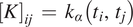 $ {\left[K\right]}_{ij}\hskip0.35em =\hskip0.35em {k}_{\alpha}\left({t}_i,{t}_j\right) $. Thus, equation (3) may alternatively be expressed as a vector Gaussian process, written here as the matrix normal distribution this induces over time
  $ t\hskip0.35em =\hskip0.35em 1,\dots, T $. Let
  $ \underset{\sim }{\boldsymbol{Y}} $ be the
  $ \left(L+1\right)\times T $ matrix representing all observed and simulated time series. Let
  $ {\mathbf{0}}_{\left(L+1\right)\times T} $ be a
  $ \left(L+1\right)\times T $ matrix of zeros. Then,
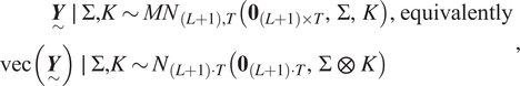 $$ {\displaystyle \begin{array}{l}\hskip3.6em \underset{\sim }{\boldsymbol{Y}}\hskip0.35em \mid \hskip0.35em \Sigma, K\sim {MN}_{\left(L+1\right),T}\left({\mathbf{0}}_{\left(L+1\right)\times T},\Sigma, K\right),\hskip0.35em \mathrm{equivalently}\\ {}\mathrm{vec}\left(\underset{\sim }{\boldsymbol{Y}}\right)\hskip0.35em \mid \hskip0.35em \Sigma, K\sim {N}_{\left(L+1\right)\cdot T}\left({\mathbf{0}}_{\left(L+1\right)\cdot T},\Sigma \hskip0.35em \otimes \hskip0.35em K\right)\end{array}}, $$
where  $ \otimes $ represents the Kronecker product.
With equation (4), standard properties of the multivariate normal distribution provide pointwise predictions and uncertainty quantification via its conditional mean and conditional variance for any subset of  $ \mathrm{vec}\left(\underset{\sim }{\boldsymbol{Y}}\right) $. In particular, let
  $ {t}_a $ corresponds to 2020 December and
  $ {t}_b $ be 2100 December. The distribution of
  $ {Y}_{0,{t}_a:{t}_b} $ conditional on the observed time series
  $ {Y}_{0,0:{t}_a} $ and CMIP6 simulations
  $ {Y}_{\mathrm{\ell},0:{t}_b} $
  $ \mathrm{\ell}\hskip0.35em =\hskip0.35em 1,\dots, L $ is also multivariate normal.
Unfortunately, the matrix  $ \Sigma \hskip0.35em \otimes \hskip0.35em K $ is quite large, with dimension
  $ \left(L+1\right)\cdot T $ by
  $ \left(L+1\right)\cdot T $. Inverting this is cubic in complexity and infeasible for large
  $ L $ or
  $ T $. Also, the manipulation of this size of matrix also incurs numerical overflow issues for sufficiently large dimension. For this final reason in particular we find it necessary to consider alternative estimation procedures.
2.3. Estimation: EB approach
While the vector Gaussian process model would lend itself to full Bayesian modeling, we propose an EB approach in order to reduce the computational overhead. Here, we describe the method by which  $ \mu (t) $ and
  $ \Sigma $ are thus estimated, and how they afford prediction and uncertainty quantification. We estimate the common mean
  $ \mu (t) $ as a Gaussian process on the time pointwise average of the model outputs
  $ {\overline{Y}}_t $. That is, define
  $ {\overline{Y}}_t\hskip0.35em =\hskip0.35em 1/\left(L+1\right){\sum}_{\mathrm{\ell}\hskip0.35em =\hskip0.35em 0}^L{Y}_{\mathrm{\ell},t} $. Then, the parameters
  $ \alpha \hskip0.35em =\hskip0.35em \left({\sigma}^2,\gamma \right) $ are estimated by maximizing the marginal likelihood of
  $ {\overline{Y}}_t $ under the Gaussian process model. Denote the estimated values of the mean function at time
  $ t $ as
  $ \hat{\mu}(t) $.
Next, take  $ {\hat{U}}_{\mathrm{\ell},t}\hskip0.35em =\hskip0.35em {Y}_{\mathrm{\ell},t}-\hat{\mu}(t) $. Then, let
  $ {\hat{\boldsymbol{U}}}_t\hskip0.35em =\hskip0.35em {\left[{\hat{U}}_{0,t}\;{\hat{U}}_{1,t}\dots {\hat{U}}_{L,t}\right]}^T $. Use
  $ {\hat{\boldsymbol{U}}}_1,\dots, {\hat{\boldsymbol{U}}}_T $ to get
  $ \hat{\Sigma} $, the
  $ \left(L+1\right)\times \left(L+1\right) $ variance–covariance matrix. This encodes the possible correlations between time series outside of the common mean, most importantly between the observed time series and the CMIP6 simulations’ outputs. Let us write
 $$ \hat{\Sigma}\hskip0.35em =\hskip0.35em \left(\begin{array}{ll}{\hat{\sigma}}_0^2& {\hat{\Sigma}}_0^T\\ {}{\hat{\Sigma}}_0& {\hat{\Sigma}}_{\mathrm{CMIP}}\end{array}\right), $$
where  $ {\hat{\sigma}}_0^2 $ is the variance of the observed data’s random effects, and
  $ {\hat{\Sigma}}_{\mathrm{CMIP}} $ is the
  $ L\times L $ covariance between random effects associated with the CMIP6 outputs.
One of our goals is to predict  $ {Y}_{0,t} $ for the months
  $ t $ spanning 2021 to 2100 given the model outputs and historic observations. The distribution of these values follows from equation (3) and standard properties of the normal distribution. Given
  $ \hat{\mu}(t) $ and simulated values
  $ {\boldsymbol{Y}}_{\mathrm{CMIP},t} $
 $$ {Y}_{0,t}\hskip0.35em \mid \hskip0.35em \hat{\mu}(t),{\boldsymbol{Y}}_{\mathrm{CMIP},t}\sim N\left({m}^{\ast },{\gamma}^{\ast}\right), $$
 $$ {m}^{\ast}\hskip0.35em =\hskip0.35em \hat{\mu}(t)+{\Sigma}_0^T{\Sigma}_{\mathrm{CMIP}}^{-1}\left({\boldsymbol{Y}}_{\mathrm{CMIP},t}-\hat{\mu}(t){\mathbf{1}}_L\right), $$
 $$ {\gamma}^{\ast}\hskip0.35em =\hskip0.35em {\sigma}_0^2-{\Sigma}_0^T{\Sigma}_{\mathrm{CMIP}}^{-1}{\Sigma}_0. $$
These conditional mean and variance values provide natural point estimates and uncertainty quantification. Note that using  $ \hat{\mu}(t) $ alone amounts to making predictions with the unconditional mean. In the next section, we will see that the conditional mean better reflects the month-to-month variation of these time series, as well as differences between them and the common mean.
3. CMIP6 Results
3.1. Leave-one-out validation
A leave-one-out (LOO) style of evaluation allows us to investigate the validity of this approach. Setting aside the observed time series  $ {Y}_{0,t} $, the remaining CMIP6 simulations all span 1850 January to 2100 December. One by one, each of the available time series is singled out and treated like the “observed” values: it is truncated to 2020 November, and we perform the model estimation approach from Section 2.3. This produces predictions through 2100, which we compare to the full-time series’s actual values.
As a typical example, Figure 1 depicts the results when the ACCESS-CM2 CMIP6 simulation is being treated like the observed time series. Our choice of highlighting this particular example is arbitrary; please see the Supplementary Material for all such cases. Predictions begin in 2020 December and continue to 2100 December. They match the actual simulated values both in broad trend across the whole of their domain, and in local month-to-month fluctuations. Note also that while the common mean function  $ \hat{\mu}(t) $ trends below the simulated values as time continues, the conditional mean (equation (7)) ameliorates this trend.

Figure 1. Amongst others, we used the ACCESS-CM2 CMIP6 time series to evaluate our model’s predictive accuracy. The top left figure shows the whole of the training and test intervals, 1850 January–2020 November and 2020 December–2100 December, respectively. Just 5 years are shown in the top right figure, starting in 2021 January, to highlight the prediction’s month-to-month accuracy. Shading (blue) indicates two standard deviations from the conditional mean, as found in equations (7) and (8). On the top and bottom left we see the conditional mean also improves predictions by inducing a trend that better matches that of the test interval compared to  $ \hat{\mu}(t) $. The correlation terms “pull” the predicted values away from
  $ \hat{\mu}(t) $ in a manner that reflects how the held-out time series’ historic values differed from the others. In the case of ACCESS-CM2, this manifests in the predicted (green) trending above
  $ \hat{\mu}(t) $ (red), which better matches the true future values.
Table 1 contains a summary of the LOO results. It includes the mean squared error (MSE) between the actual output of the indicated simulation and the predictions of our EB model. We compare our method to the predictions found using just the common mean function  $ \hat{\mu}(t) $ and using the pointwise average
  $ {\overline{Y}}_t $. The former amounts to only fitting the Gaussian process, omitting the random effects
  $ \boldsymbol{U}(t) $. The pointwise average merely takes the means of all training forecasts. The empirical Bayes model has a lower MSE than the common mean in every case.
Table 1. Each CMIP6 simulation was treated like the observed time series, truncated to 2020 November, and predicted by various methods.

Note. The predictions produced by our empirical Bayes model are similar in accuracy to using  $ {\overline{Y}}_t $ itself and also provide an estimate of variability. These predictions were superior to the common mean component
  $ \hat{\mu}(t) $ on every CMIP6 test simulation.
3.2. Observed time series
Making predictions for the observed climate follows the procedure in Section 2.3. Figure 2 depicts the predicted values for the observed time series  $ {Y}_{0,t} $ from 2020 December–2100 December. The upward trend is driven by the common mean
  $ \hat{\mu}(t) $ estimated on the CMIP6 time series. The random effects induce the month-to-month variations, shown in Section 3.1 to better reflect CMIP6 time series.

Figure 2. Predicted values for mean global surface temperature using equation (7), with shading to  $ \pm 2 $ standard deviations (equation (8)). This model leverages the common mean as well as individual correlations amongst CMIP6 simulations and historical observed data.
Note that the observed time series has less variation than the CMIP6 simulations considered here. Over the shared period of 1850 January to 2020 November, the observed time series has a variance of 0.15 compared to 0.55 for the CMIP6 simulations on average. Comparing Figure 2 to the ACCESS-CM2 data in Figure 1 is representative of this. This is then reflected in the covariance matrix equation (5); its attenuating presence in equation (7) explains how the predictions in Figure 2 show less variation than those in Figure 1.
4. Conclusion
This preliminary investigation affirms the use of our hierarchical Bayesian model in combining multimodel climate data. Our model reflects both the small and large-scale deviational properties of a given time series vis–a-vis a common mean. An EB treatment is an attractive approach to estimating this model; additional climate simulations can be considered with little added computational cost. This is especially important in applications where simulations produce high-dimensional output as is common in climate science.
Our model assumes that the properties of the common trend  $ \mu \left(\cdot \right) $ can be adequately captured using a Gaussian process. This can be easily extended to a
  $ t $-process or an elliptically contoured process with some additional computations. Also, our model extends to the case where there is a spatial component in the data or where we consider regional climate models: the principles outlined above extend simply to such cases.
Acknowledgments
We are grateful for the considerate input of our reviewers which aided in the clarity of this manuscript.
Author Contributions
Conceptualization: M.T., S.C.; Data curation: A.B.; Formal analysis: M.T.; Methodology: M.T., S.C.; Software: M.T.; Supervision: A.B., S.C.; Writing—original draft: M.T.; Writing—review and editing: S.C.
Competing Interests
The authors declare no competing interests exist.
Data Availability Statement
All materials and code necessary to reproduce these results may be found at https://github.com/MartenThompson/climate_informatics_2022. Please see relevant citations in Section 1 for CMIP6 and observed data.
Ethics Statement
The research meets all ethical guidelines, including adherence to the legal requirements of the study country.
Funding Statement
This research is partially supported by the US National Science Foundation (NSF) under grants 1939916, 1939956, and a grant from Cisco Systems, Inc. It was carried out partially at the Jet Propulsion Laboratory, California Institute of Technology, under a contract with the National Aeronautics and Space Administration (80NM0018D0004).
Provenance
This article is part of the Climate Informatics 2022 proceedings and was accepted in Environmental Data Science on the basis of the Climate Informatics peer review process.
Supplementary Materials
To view supplementary material for this article, please visit http://doi.org/10.1017/eds.2022.24.


 Open access