


1. Introduction: the context in design
Robust parameter design is an off-line quality control method whose purpose is to reduce the variability in performance of products and processes in the face of uncontrollable variations in the environment, manufacture, internal degradation and usage conditions (Taguchi Reference Taguchi1987; Phadke Reference Phadke1989; Wu & Hamada Reference Wu and Hamada2000). The variables that affect a product’s response are classified into control factors whose nominal settings can be specified and noise factors that cause unwanted variations in the system response. In robust design, the space of control factors is searched to seek settings that are less sensitive to the noise factors and therefore exhibit less variation in performance.
Robust parameter design is increasingly performed using computer models of the product or process rather than laboratory experiments. Computer models can provide significant advantages in cost and speed of the robustness optimization process. Although random variations in noise factors can be simulated in a computer, the results of computer models generally lack pure experimental error (Simpson et al. Reference Simpson, Peplinski, Koch and Allen2001). Therefore, it is generally acknowledged that the techniques for robust design via computer models ought to be different than the techniques for robust design via laboratory experiments. In response to this fact, the field of design and analysis of computer experiments (DACE) has grown rapidly in recent decades providing a variety of useful techniques (Santner et al. Reference Santner, Williams and Notz2003). A review of the emerging field of DACE was provided by Giunta et al. (Reference Giunta, Wojtkiewicz and Eldred2003). Three of the most promising techniques developed so far are reviewed in the next paragraphs.
Robust design with computer experiments is often accomplished using a strategy employing two nested loops as depicted in Figure 1, an inner sampling loop and an outer optimization loop (Kalagnanam & Diwekar Reference Kalagnanam and Diwekar1997; Du & Chen Reference Du and Chen2002; Lu & Darmofal Reference Lu and Darmofal2005). The goal of robust design with computer experiments is to determine the optimal setting of control factors that minimizes the variance of the probabilistic model, while ensuring that the mean of the probabilistic model remains at the target value. The mean and variance are calculated by repeatedly running the deterministic computer model with different values of noise factors which are generated by a sampling scheme. Thus, the inner sampling loop comprises the probabilistic model and the outer optimization loop serves to decrease the variance of the probabilistic model’s output.
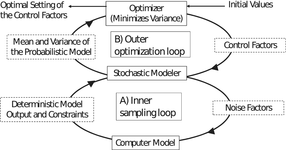
Figure 1. Schematic description of robust design including a sampling loop embedded within an optimization loop (Adapted from Kalagnanam & Diwekar Reference Kalagnanam and Diwekar1997).
2. Ways to implement the inner sampling loop
LHS is a stratified sampling technique that can be viewed as an extension of Latin square sampling and a close relative of highly fractionalized factorial designs (McKay et al. Reference McKay, Beckman and Conover1979). LHS ensures that each input variable has all portions of its distributions represented by input values. This is especially advantageous when only a few of the many inputs turn out to contribute significantly to the output variance. It has been proven that, for large samples, LHS provides smaller variance in estimators than simple random sampling as long as the response function is monotonic in all the noise factors (McKay et al. Reference McKay, Beckman and Conover1979). In typical engineering applications, LHS converges to 1% accuracy in estimating variance in about 2000 samples. However, there is also evidence that LHS provides no significant practical advantage over simple random sampling if the response function is highly nonlinear (Giunta et al. Reference Giunta, Wojtkiewicz and Eldred2003) so the number of samples required to converge to 1% will sometimes be much larger than 2000. Latin hypercube design continues to be an active area of improvement. Chen and Xiong (Reference Chen and Xiong2017) proposed a means to nest these designs so that sequential construction is enabled and the restriction to multiples of the original design is relaxed. With similar objectives, Kong et al. (Reference Kong, Ai and Tsui2018) proposed new sliced designs that accommodate arbitrary sizes for different slices and also derived their sampling properties.
An innovation called Hammersley sequence sampling (HSS) appears to provide significant advantages over LHS (Kalagnanam & Diwekar Reference Kalagnanam and Diwekar1997). HSS employs a quasi-Monte Carlo sequence with low discrepancy and good space-filling properties. In applications to simple functions, it has been demonstrated that HSS converges to 1% accuracy faster than LHS by a factor of from 3 to 100. In an engineering application, HSS converged to 1% accuracy in about 150 samples.
A methodology based on the quadrature factorial model (QFM) employs fractional factorial designs augmented with a center point as a sampling scheme. A local regression model is formed based on these samples. This model is then used to generate the missing samples from a “contrived” full factorial 3k design. Finally, this 3k design is used to estimate the expected performance and deviation index. This method was shown to produce reasonable estimates with fewer samples especially for systems with significant interaction effects and nonlinear behavior (Yu & Ishii Reference Yu and Ishii1998).
Quadrature and cubature are techniques for exactly integrating specified classes of functions by means of a small number of highly structured samples. A remarkable number of different methods have been proposed for different regions and weighting functions (see Cools & Rabinowitz (Reference Cools and Rabinowitz1993) and Cools (Reference Cools1999), for reviews). More recently, Lu & Darmofal (Reference Lu and Darmofal2005) developed a cubature method for Gaussian weighted integration that scales better than other, previously published cubature schemes. If the number of uncertain factors in the inner loop is m, then the method requires m 2 + 3m + 3 samples. The new rule provides exact solutions for the mean for polynomials of fifth degree including the effects of all multifactor interactions. Used recursively to estimate transmitted variance, it provides exact solutions for polynomials of second degree including all two-factor interactions. On a challenging engineering application, the cubature method had less than 0.1% error in estimating mean and about 1% to 3% error in estimating variance. Quadratic scaling with dimensionality limits the method to applications with a relatively small number of uncertain factors.
A meta-model approach has been widely used in practice to overcome computational complexity (Booker et al. Reference Booker, Dennis, Serafini, Torczon and Trosset1999; Simpson et al. Reference Simpson, Peplinski, Koch and Allen2001; Hoffman et al. Reference Hoffman, Sudjianto, Du and Stout2003; Du et al. Reference Du, Sudjianto and Chen2004). The term “meta-model” denotes a user-defined cheap-to-compute function which approximates the computationally expensive model. The popularity of the meta-model approach is due to (1) the cost of computer models of high fidelity in many engineering applications and (2) the many runs that are required for robust design, for which direct computing may be prohibitive. Although the meta-model approach has become a popular choice in many engineering designs, it does have some limitations. One difficulty associated with the meta-model approach is the challenge of constructing an accurate meta-model to represent the original model from a small sample size (Jin et al. Reference Jin, Chen and Simpson2000; Ye et al. Reference Ye, Li and Sudjianto2000). These meta-model-based approaches continue to be improved and integrated with the optimization process (a departure from the nested loop structure displayed in Figure 1). For example, Iooss & Marrel (Reference Iooss and Marrel2019) combined several statistical tools including space-filling design, variable screening and Gaussian process metamodeling. The combined approach enabled consideration of a large number of variables and a more accurate estimation of confidence intervals for the results.
In meta-model-based approaches to robust design, acquisition functions are often used to sequentially determine the next design point so that a Gaussian Process emulator can more accurately locate the optimal setting. Tan (Reference Tan2020) proposed four new acquisition functions for optimizing expected quadratic loss, analyzed their convergence and developed accurate methods to compute them. Tan applied acquisition functions to robust parameter design problems with internal noise factors based on a Gaussian process model and an initial design tailored for such problems. On relatively simple functions, the proposed methods outperformed an optimization approach based on modeling the quadratic loss as a Gaussian Process and also performed better than maximin Latin hypercube designs. However, the proposed methods do not scale well to a large number of noise factors.
A method for robust parameter design using computer models was proposed by Tan & Wu (Reference Tan and Wu2012) using a Bayesian framework and Gaussian process meta-models. They proposed an expected quadratic loss criterion derived by taking expectation with respect to the noise factors and the posterior predictive process. An advantage of the approach is that it provides accurate Bayesian credible intervals for the average quadratic loss. This is valuable because the practitioner will benefit from not only a recommended set point for the control factors but also an interval estimate for the quality loss. These credible intervals are constructed via numerical inversion of the Lugannani–Rice saddlepoint approximation. A relationship between the quadrature method proposed here and the Tan and Wu approach is that integration required for computing the credible intervals used a three- or four-point quadrature method for evaluating the integral needed to find the cumulative density function for quadratic loss. An important difference is that Tan and Wu assumed that the distribution of the noise factors is discrete, or can be discretized. By contrast, the method proposed here assumes that the noise factors are normally distributed or else that they are adequately represented for the purpose of robust parameter design by their first two moments. Also, instead of confidence intervals on quadratic loss, our method provides an estimate of mean and variance of the error of its results.
Joseph et al. (Reference Joseph, Gul and Ba2020) proposed a method for robust design with computer experiments with particular emphasis on nominal, discrete, and ordinal factors. The experimental designs are constructed to follow a maximum projection criterion which can simultaneously optimize the space-filling properties of the design points. This was an important development for instances when various types of factors are mixed in the problem domain because the optimal design criterion incorporating different types of input factors can produce much better experimental designs.
3. Motivation for this paper
The motivation for this paper is that LHS and HSS still require too many samples for many practical engineering applications. Computer models of adequate fidelity can require hours or days to execute. In some cases, changing input parameters to the computer models is not an automatic process – it can often require careful attention to ensure that the assumptions and methods of the analysis remain reasonable. It is also frequently the case that the results of computer models must be reviewed by experts or that some human intervention is required to achieve convergence. All of these considerations suggest a demand for techniques requiring a very small number of samples. Although QFM is designed to meet these needs, further improvements seem to be desirable.
Based on the considerations presented above, Frey et al. (Reference Frey, Reber and Lin2005) were motivated to develop a technique for computer experiments requiring a very small number of samples. They found that a five-point quadrature formula could be extended to multiple dimensions resulting in a 4d + 1 formula that provided generally very good outcomes. Using case studies and a model-based evaluation, they showed that the quadrature technique can estimate the standard deviation within 5% in over 95% of systems which is far superior to LHS or HSS. Cubature performs somewhat better than quadrature with a similar number of samples given low dimensional problems, but cubature scales with the square of the dimension rather than linearly.
A concern regarding the quadrature-based technique is that its theoretical foundations were unclear. In particular, the extension to multiple dimensions seemed to be poorly justified. Therefore, the empirically demonstrated performance of the method presents a puzzle. This paper is the result of our efforts to establish a theoretical foundation and enable practitioners to better understand the assumptions required for its use.
4. Single variable Hermite–Gauss formula
As discussed in the introduction, robust parameter design requires a procedure to estimate the variance of the response of an engineering system in the presence of noise factors. Estimating the variance of a function involves computing an integral. One basic integration technique is Hermite–Gaussian quadrature. First, let us consider a one-dimensional case. Let us denote the response of the system as y and a single noise factor as z. If the noise factor is a standard normal variate, then the expected value of y can be estimated by a five-point Hermite–Gaussian quadrature formula. Figure 2 describes the concept as applied to an arbitrary function y(z) and depicting the noise factor z as having zero mean to simplify the graphic.
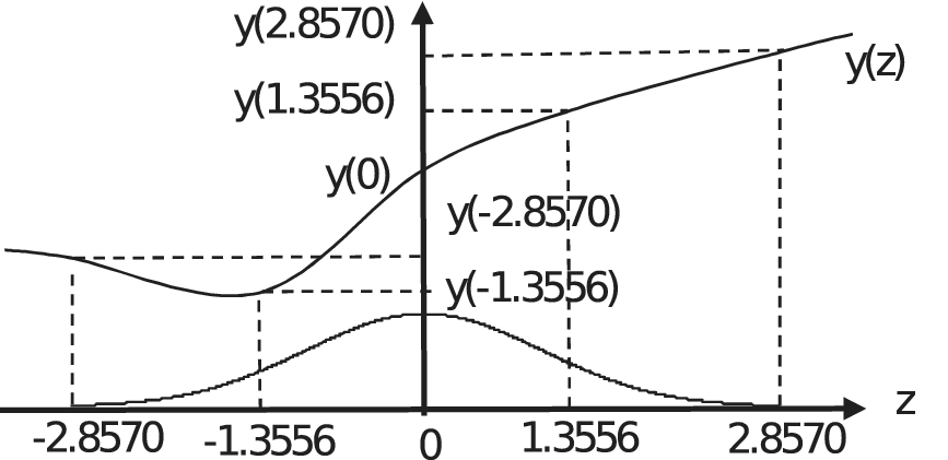
Figure 2. Five-point Hermite–Gauss Quadrature applied to an arbitrary function with the noise factor shifted and scaled to have zero mean and unit variance.
The function is sampled at five points. One sample is at the mean of the variable z which is zero for this example. The other four samples are distributed symmetrically about the origin at prescribed points. The values of the function y(z) are weighted and summed to provide an estimate of the expected value. The sample points and weights in the following equation are selected so that the Hermite–Gaussian quadrature formula gives exact results if y(z) is a polynomial of degree nine or less (Stroud & Seacrest Reference Stroud and Seacrest1966). The five-point Hermite–Gaussian quadrature formula is
 $$ {\displaystyle \begin{array}{l} Ey(z)\Big)=\underset{-\infty }{\overset{\infty }{\int }}\frac{1}{\sqrt{2\pi }}{e}^{-\frac{1}{2}{z}^2}y(z) dz\approx \\ {}y(0)+\frac{1}{\sqrt{\pi }}\left[\begin{array}{l}{A}_1\left[y\left({\zeta}_1\right)-y(0)\right]+{A}_1\left[y\left(-{\zeta}_1\right)-y(0)\right]+\\ {}{A}_2\left[y\left({\zeta}_2\right)-y(0)\right]+{A}_2\left[y\left(-{\zeta}_2\right)-y(0)\right]\end{array}\right],\end{array}} $$
with weights  $ {A}_1=0.39362\;\left(=\frac{1}{60}\left(7+2\sqrt{10}\right)\sqrt{\pi}\right) $,
  $ {A}_2=0.019953\;\left(=\frac{1}{60}\left(7-2\sqrt{10}\right)\sqrt{\pi}\right) $ and sample points
  $ {\unicode{x03B6}}_1=1.3556\;\left(=\sqrt{5-\sqrt{10}}\right) $ and
  $ {\unicode{x03B6}}_2=2.8570\;\left(=\sqrt{5+\sqrt{10}}\right) $.
Estimating variance also involves computing an expected value, namely  $ E\left[{\left(y(z)-E\left[y(z)\right]\right)}^2\right] $. By using Eq. (1) recursively, a variance estimate can be made using the same five samples although the approach gives exact results only if y(z) is a polynomial of degree four or less.
 $$ {\displaystyle \begin{array}{l}E\left[{\left(y(z)-E\left[y(z)\right]\right)}^2\right]=\underset{-\infty }{\overset{\infty }{\int }}\frac{1}{\sqrt{2\pi }}{e}^{-\frac{1}{2}{z}^2}{\left(y(z)-E\left[y(z)\right]\right)}^2 dz\\ {}\hskip0.48em \approx {\left[y(0)-E\left(y(z)\right)\right]}^2+\\ {}\hskip0.48em \frac{1}{\sqrt{\pi }}\left[\begin{array}{l}{A}_1\left[{\left(y\left({\zeta}_1\right)-E\left(y(z)\right)\right)}^2-{\left(y(0)-E\left(y(z)\right)\right)}^2\right]+\\ {}{A}_1\left[{\left(y\left({\zeta}_1\right)-E\left(y(z)\right)\right)}^2-{\left(y(0)-E\left(y(z)\right)\right)}^2\right]+\\ {}{A}_2\left[{\left(y\left({\zeta}_2\right)-E\left(y(z)\right)\right)}^2-{\left(y(0)-E\left(y(z)\right)\right)}^2\right]+\\ {}{A}_2\left[{\left(y\left(-{\zeta}_2\right)-E\left(y(z)\right)\right)}^2-{\left(y(0)-E\left(y(z)\right)\right)}^2\right]\end{array}\right]\\ {}\hskip0.48em =\frac{1}{\sqrt{\pi }}\left[\begin{array}{l}{A}_1\left[{\left(y\left({\zeta}_1\right)-y(0)\right)}^2+{\left(y\left(-{\zeta}_1\right)-y(0)\right)}^2\right]+\\ {}{A}_2\left[{\left(y\left({\zeta}_2\right)-y(0)\right)}^2+{\left(y\left(-{\zeta}_2\right)-y(0)\right)}^2\right]\end{array}\right]\\ {}\hskip0.48em -\frac{1}{\sqrt{\pi }}{\left[\begin{array}{l}{A}_1\left(y\left({\zeta}_1\right)+y\left(-{\zeta}_1\right)\right)-2\left(y(0)\right)+\\ {}{A}_2\left(y\left({\zeta}_2\right)+y\left(-{\zeta}_2\right)\right)-2\left(y(0)\right)\end{array}\right]}^2.\end{array}} $$
5. Multiple variables Hermite–Gauss formula
In the multidimensional case, estimation of integrals becomes more complex. A variety of cubature formulae for Gaussian weighted m-dimensional integrals have been derived (Stroud Reference Stroud1971). These cubature techniques all scale poorly with the dimensionality of the integral despite recent improvements. For responses with more than about 10 variables, cubature will require too many samples to meet the stated goals.
To circumvent the problem of scaling in multidimensional integrals, it is proposed that a one-dimensional quadrature rule can be adapted to m-dimensional problems. The expected value of a function y is approximated by
 $$ E\left(y(z)\right)\approx y\left(\overline{z}\right)+\sum \limits_{i=1}^m\sum \limits_{j=1}^{i-1}{\alpha}_i^{\left(, j\right)}\left[y\left({\mathbf{D}}_i^{\left(, j\right)}{e}_i+\overline{z}\right)-y\left(\overline{z}\right)\right], $$
 $$ {e}_i=\left[{\delta}_{1i}\hskip0.5em {\delta}_{2i}\;\begin{array}{cc}\cdots & {\delta}_{ni}\end{array}\right]\hskip1em \mathrm{and}\hskip1em {\delta}_{ni}=\left\{\begin{array}{c}0\hskip1em \mathrm{if}\hskip1em i\ne j,\\ {}1\hskip1em \mathrm{if}\hskip1em i=j,\end{array}\right. $$
The variance of the function y is approximated by
 $$ {\sigma}^2\left(y(z)\right)\approx \sum \limits_{i=1}^m\left[{\left(y\left(\overline{z}\right)+\sum \limits_{j=1}^{i-1}{\alpha}_i^{\left(, j\right)}\left[y\left({D}_i^{\left(, j\right)}+\overline{z}\right)-y\left(\overline{z}\right)\right]\right)}^2-\left[{y}^2\left(\overline{z}\right)+\sum \limits_{i=1}^m\sum \limits_{j=1}^{i-1}{\alpha}_i^{\left(, j\right)}\left[{y}^2\left({D}_i^{\left(, j\right)}+\overline{z}\right)-{y}^2\left(\overline{z}\right)\right]\right]\right], $$
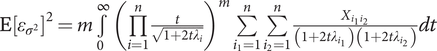
where D〈i〉 denotes the ith row of the design matrix D. For the quadrature-based method with 4m + 1 samples and the design matrix D is
 $$ \mathbf{D}=\left[\frac{\frac{+{\zeta}_1\cdot \mathbf{I}}{-{\zeta}_1\cdot \mathbf{I}}}{\frac{+{\zeta}_2\cdot \mathbf{I}}{-{\zeta}_2\cdot \mathbf{I}}}\right],\hskip0.84em \mathbf{I}={\left[\begin{array}{ccc}1& & 0\\ {}& \ddots & \\ {}0& & 1\end{array}\right]}_{m\times m}. $$
This requires 4m + 1 samples. The values of A 1 and A 2 and of ζ1 and ζ2 are the same as in the one-dimensional case.
A graphical depiction of the design for three standard normal variables (m = 3) and using 4m + 1 samples is presented in Figure 3. The sampling scheme is composed of one center point and four axial runs per variable. Thus, the sampling pattern is similar to a star pattern in a central composite design.
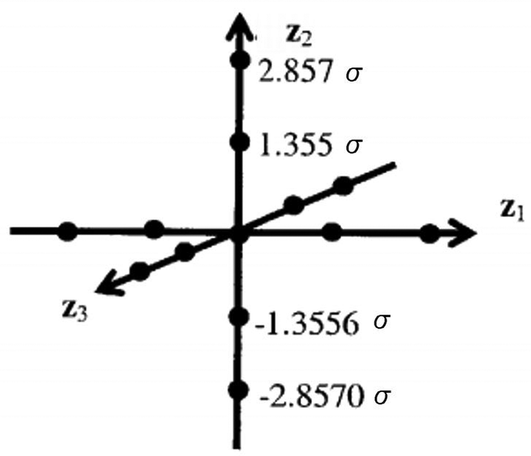
Figure 3. The sampling arrangement of the proposed quadrature-based method.
6. Developing expressions for the method’s error
The accuracy of the Hermite–Gaussian quadrature method in estimating the mean and variance can be verified using a Taylor series expansion.
In accordance with the previous sections, the accuracy of the Hermite–Gaussian quadrature method is first illustrated for a function of only one noise factor following a standard normal distribution. If the response function y(z) is continuous and differentiable, then the Taylor series approximation of y(z) at z = 0 is
 $$ y(z)=y(0)+{y}^{(1)}(0)z+\frac{y^{(2)}(0)}{2!}{z}^2+\frac{y^{(3)}(0)}{3!}{z}^3+\cdots . $$
For legibility reasons, from now on  $ \frac{y^{(i)}(0)}{i!} $, which is the polynomial coefficient of zi, is replaced by
  $ {\beta}^{(i)} $. With z ~ N(0,1), if the coefficients were known, the exact expected value of y(z) could be calculated as
 $$ {\displaystyle \begin{array}{c}E\left[y(z)\right]=\frac{1}{\sqrt{2\pi }}\underset{-\infty }{\overset{\infty }{\int }}{e}^{-\frac{1}{2}{z}^2}\sum \limits_{n=0}^{\infty }{\beta}^{(n)}{z}^n dz\\ {}=\frac{1}{\sqrt{2\pi }}\sum \limits_{n=0}^{\infty }{\beta}^{(n)}\underset{-\infty }{\overset{\infty }{\int }}{e}^{-\frac{1}{2}{z}^2}{z}^n dz\\ {}=\frac{1}{\sqrt{2\pi }}\sum \limits_{k=0}^{\infty }{\beta}^{(2k)}\underset{-\infty }{\overset{\infty }{\int }}{e}^{-\frac{1}{2}{z}^2}{z}^{2k} dz\hskip-5.5pt \\ {}\hskip2pc =\sum \limits_{k=0}^{\infty}\frac{(2k)!}{2^kk!}{\beta}^{(2k)}.\hskip3.8pc \end{array}} $$
In contrast, the expected value of y(z) can also be estimated using the quadrature-based method, again using the Taylor series of y(z),
 $$ {\displaystyle \begin{array}{c}E\left(y(z)\right)=\underset{-\infty }{\overset{\infty }{\int }}\frac{1}{\sqrt{2\pi }}{e}^{-\frac{1}{2}{z}^2}y(z) dz\hskip10.7pc \\ {}\approx y(0)+\frac{1}{\sqrt{\pi }}\left[\begin{array}{l}{A}_1\left[y\left({\zeta}_1\right)-y(0)\right]+{A}_1\left[y\left(-{\zeta}_1\right)-y(0)\right]+\\ {}{A}_2\left[y\left({\zeta}_2\right)-y(0)\right]+{A}_2\left[y\left(-{\zeta}_2\right)-y(0)\right]\end{array}\right]\\ {}=y(0)+\frac{2}{\sqrt{\pi }}\left[\sum \limits_{k=1}^{\infty }{\beta}^{(2k)}\left[{A}_1{\zeta}_1^{2k}+{A}_2{\zeta}_2^{2k}\right]\right].\hskip4.6pc \end{array}} $$
Elaboration of Eq. (7) yields
 $$ {\displaystyle \begin{array}{c}\hskip-2pc E{\left[y(z)\right]}_{\mathrm{exact}}={\beta}^{(0)}+{\beta}^{(2)}+3{\beta}^{(4)}+15{\beta}^{(6)}+\\ {}105{\beta}^{(8)}+945{\beta}^{(10)}+10395{\beta}^{(12)}+\cdots .\hskip-2.7pc \end{array}} $$
Elaboration of Eq. (8) yields
 $$ {\displaystyle \begin{array}{c}E{\left[y(z)\right]}_{\mathrm{quadr}}={\beta}^{(0)}+{\beta}^{(2)}+3{\beta}^{(4)}+15{\beta}^{(6)}+\\ {}105{\beta}^{(8)}+825{\beta}^{(10)}+6675{\beta}^{(12)}+\cdots .\hskip-2.4pc \end{array}} $$
The coefficients of the first five terms are equal. Therefore, for polynomials of degree less than 9 the quadrature method will give exact solutions.
Substituting the Taylor series approximation of y(z) at z = 0 allows the exact value of variance of y(z) to be expressed as a function of the coefficients:
 $$ {\displaystyle \begin{array}{c}\operatorname{var}\left(y(z)\right)=\frac{1}{\sqrt{2\pi }}\underset{-\infty }{\overset{\infty }{\int }}{e}^{-\frac{1}{2}{z}^2}{y}^2(z) dz-{\left[\frac{1}{\sqrt{2\pi }}\underset{-\infty }{\overset{\infty }{\int }}{e}^{-\frac{1}{2}{z}^2}y(z) dz\right]}^2\\ {}=\sum \limits_{k=0}^{\infty}\frac{(2k)!}{2^kk!}\sum \limits_{i=0}^{2k}{\beta}^{(i)}{\beta}^{\left(2k-i\right)}-{\left[\sum \limits_{k=0}^{\infty}\frac{(2k)!}{2^kk!}{\beta}^{(2k)}\right]}^2,\hskip1.5pc \end{array}} $$
The variance of y(z) can also be estimated using the quadrature-based method,
 $$ {\displaystyle \begin{array}{c}\operatorname{var}\left(y(z)\right)\approx \frac{1}{\sqrt{\pi }}\left[\begin{array}{l}{A}_1\left[{\left(y\left({\zeta}_1\right)-y(0)\right)}^2+{\left(y\left(-{\zeta}_1\right)-y(0)\right)}^2\right]+\\ {}{A}_2\left[{\left(y\left({\zeta}_2\right)-y(0)\right)}^2+{\left(y\left(-{\zeta}_2\right)-y(0)\right)}^2\right]\end{array}\right]\\ {}-\frac{1}{\pi }{\left[\begin{array}{l}{A}_1\left(y\left({\zeta}_1\right)+y\left(-{\zeta}_1\right)-2y(0)\right)+\\ {}{A}_2\left(y\left({\zeta}_2\right)+y\left(-{\zeta}_2\right)-2y(0)\right)\end{array}\right]}^2\hskip52pt \\ {}=\frac{2}{\sqrt{\pi }}\left[\sum \limits_{k=1}^{\infty}\left(\sum \limits_{j=1}^{2k-1}{\beta}^{\left(, j\right)}{\beta}^{\left(2k-j\right)}\right)\left[{A}_1{\zeta}_1^{2k}+{A}_2{\zeta}_2^{2k}\right]\right]\hskip1.5pc \\ {}-\frac{4}{\pi }{\left[\sum \limits_{k=1}^{\infty }{\beta}^{(2k)}\left[{A}_1{\zeta}_1^{2k}+{A}_2{\zeta}_2^{2k}\right]\right]}^2.\hskip6.2pc \end{array}} $$
Elaboration of Eq. (11) yields
 $$ {\displaystyle \begin{array}{c}\operatorname{var}{\left(y(z)\right)}_{\mathrm{exact}}={\left({\beta}^{(1)}\right)}^2+\left(6{\beta}^{(1)}{\beta}^{(3)}+2{\left({\beta}^{(2)}\right)}^2\right)+\left(30{\beta}^{(1)}{\beta}^{(5)}+24{\beta}^{(2)}{\beta}^{(4)}+15{\left({\beta}^{(3)}\right)}^2\right)+\\ {}\left(210{\beta}^{(1)}{\beta}^{(7)}+180{\beta}^{(2)}{\beta}^{(6)}+210{\beta}^{(3)}{\beta}^{(5)}+96{\left({\beta}^{(4)}\right)}^2\right)+\hskip6.78pc \\ {}\left(1890{\beta}^{(1)}{\beta}^{(9)}+1680{\beta}^{(2)}{\beta}^{(8)}+1890{\beta}^{(3)}{\beta}^{(7)}+1800{\beta}^{(4)}{\beta}^{(6)}+945{\left({\beta}^{(5)}\right)}^2\right)+\cdots .\hskip-.85pc \end{array}} $$
Elaboration of Eq. (12) yields
 $$ {\displaystyle \begin{array}{c}\operatorname{var}{\left(y(z)\right)}_{\mathrm{exact}}={\left({\beta}^{(1)}\right)}^2+\left(6{\beta}^{(1)}{\beta}^{(3)}+2{\left({\beta}^{(2)}\right)}^2\right)+\left(30{\beta}^{(1)}{\beta}^{(5)}+24{\beta}^{(2)}{\beta}^{(4)}+15{\left({\beta}^{(3)}\right)}^2\right)+\\ {}\left(210{\beta}^{(1)}{\beta}^{(7)}+180{\beta}^{(2)}{\beta}^{(6)}+210{\beta}^{(3)}{\beta}^{(5)}+96{\left({\beta}^{(4)}\right)}^2\right)+\hskip6.75pc \\ {}\left(1650{\beta}^{(1)}{\beta}^{(9)}+1440{\beta}^{(2)}{\beta}^{(8)}+1650{\beta}^{(3)}{\beta}^{(7)}+1560{\beta}^{(4)}{\beta}^{(6)}+825{\left({\beta}^{(5)}\right)}^2\right)+\cdots .\hskip-.9pc \end{array}} $$
The coefficients of the first 10 terms are equal. Therefore, for polynomials of degree less than 5, the quadrature method will give exact solutions for the variance.
Now consider the case for m random input variables, all independent and following a standard normal distribution (without loss of generality because scaling and shifting of the variable z is accomplished relatively simply). Assuming the function is separable, y(z) can be written as  $ \sum \limits_{j=1}^m{y}_j\left({z}_j\right) $.
To simplify notation, from this point forward,  $ \frac{1}{i!}\frac{\partial^iy}{\partial {z}_j^i}\left(\underline{0}\right) $, which is the polynomial coefficient of
  $ {z}_j^i $, is replaced by
  $ {\beta}_j^{(i)} $.
In that case, the Taylor series approximation of y(z) around z = (0, 0, …, 0) is
 $$ y(z)=y(0)+\sum \limits_{n=1}^{\infty}\sum \limits_{j=1}^m\left[{\beta}_j^{(n)}{z}_j^n\right]. $$
And corresponding with Eq. (7) the expected value of y(z) equals
 $$ E\left[y(z)\right]=y(0)+\sum \limits_{k=1}^{\infty}\frac{(2k)!}{2^kk!}\sum \limits_{j=1}^m{\beta}_j^{(2k)}. $$
Using the quadrature-based method, the expected value of y(z) can also be estimated,
 $$ {\displaystyle \begin{array}{c}E\left(y\left(\underline{z}\right)\right)=\sum \limits_{j=1}^mE\left({y}_j\left({z}_j\right)\right)\hskip8.9pc \\ {}\approx \hskip1.5pt y\left(\underline{0}\right)+\frac{2}{\sqrt{\pi }}\sum \limits_{j=1}^m\left[\sum \limits_{k=1}^{\infty}\left[{A}_1{\zeta}_1^{2k}+{A}_2{\zeta}_2^{2k}\right]{\beta}_j^{(2k)}\right].\end{array}} $$
Elaboration of both Eqs. (14) and (15) gives a similar result as in the one-dimensional case. For continuous, differentiable and separable polynomials of degree less than 10 the quadrature method will give exact solutions for the expected value.
The relative error mean is obtained by subtracting Eq. (15) from Eq. (14) and then dividing by Eq. (14).
 $$ \begin{array}{c}\hskip-20.5pc \mathrm{Rel}\_\mathrm{error}=\\ {}\frac{-{\sum}_{\hskip0pt j=1}^m\left[120{\beta}_j^{(10)}+3720{\beta}_j^{(12)}+\dots \right]}{y\left(\overline{\underline{z}}\right)+{\sum}_{\hskip0pt j=1}^m\left[{\beta}_j^{(2)}+3{\beta}_j^{(4)}+15{\beta}_j^{(6)}+105{\beta}_j^{(8)}+945{\beta}_j^{(10)}+10395{\beta}_j^{(12)}+\dots \right]}.\end{array} $$
The coefficients in the numerator are typically very small. And it is also likely that the term y( $ \overline{z} $) in the denominator is the dominating term in practical engineering systems. Hence the quadrature-based method gives accurate results in estimating the expected value for 10th or higher order separable polynomial systems.
Corresponding with Eq. (11), the variance of y(z) equals
 $$ \operatorname{var}\left(y(z)\right)=\sum \limits_{j=1}^m\left[\sum \limits_{k=0}^{\infty}\frac{(2k)!}{2^kk!}\sum \limits_{i=0}^{2k}{\beta}_j^{(i)}{\beta}_j^{\left(2k-i\right)}-{\left[\sum \limits_{k=0}^{\infty}\frac{(2k)!}{2^kk!}{\beta}_j^{(2k)}\right]}^2\right]. $$
Using the quadrature-based method, the variance of y(z) can also be estimated
 $$ \operatorname{var}\left(y(z)\right)\approx \left[\sum \limits_{j=1}^m\begin{array}{l}\frac{2}{\sqrt{\pi }}\left[\sum \limits_{k=1}^{\infty}\left(\sum \limits_{i=1}^{2k-1}{\beta}_j^{(i)}{\beta}_j^{\left(2k-i\right)}\right)\left[{A}_1{\zeta}_1^{2k}+{A}_2{\zeta}_2^{2k}\right]\right]\\ {}-\frac{4}{\pi }{\left[\sum \limits_{k=1}^{\infty }{\beta}_j^{(2k)}\left[{A}_1{\zeta}_1^{2k}+{A}_2{\zeta}_2^{2k}\right]\right]}^2\end{array}\right]. $$
The relative error mean is obtained by subtracting Eq. (18) from Eq. (17) and then divided by Eq. (17)
 $$ {\varepsilon}_{\sigma^2}=\sum \limits_{j=1}^m\frac{-240\left({\beta}_j^{(1)}{\beta}_j^{(9)}+{\beta}_j^{(2)}{\beta}_j^{(8)}+{\beta}_j^{(3)}{\beta}_j^{(7)}+{\beta}_j^{(4)}{\beta}_j^{(6)}+\frac{1}{2}{\left({\beta}_j^{(5)}\right)}^2\right)-\cdots }{{\left({\beta}_j^{(1)}\right)}^2+\left(6{\beta}_j^{(1)}{\beta}_j^{(3)}+2{\left({\beta}_j^{(2)}\right)}^2\right)+\left(30{\beta}_j^{(1)}{\beta}_j^{(5)}+24{\beta}_j^{(2)}{\beta}_j^{(4)}+15{\left({\beta}_j^{(3)}\right)}^2\right)+\cdots }. $$
The coefficients in the numerator are again small. Hence the quadrature-based method gives accurate results in estimating the variance for 5th or higher order separable polynomial systems.
7. Statistical properties of error
For the following results, we assume continuous, differentiable and separable polynomials with polynomial coefficients that are mutually independent and normally distributed with zero mean and variances that decrease geometrically at rate r with the increasing of polynomial order, that is,  $ {\beta}_j^{(i)}\sim N\left(0,{r}^i\right) $.
For polynomials satisfying these properties, we can derive exact formulas for the expected value and the variance of the error  $ {\varepsilon}_{\sigma^2} $ in Eq. (19). Essential to this effort is a theorem proved by Magnus (Reference Magnus1986), which will be presented in its entirety here.
Theorem 1 (Magnus Reference Magnus1986)
Let x be a normally distributed n × 1 vector with mean μ and positive definite covariance matrix Ω = LLT. Let A be a symmetric n × n matrix and B a positive semidefinite n × n matrix, B ≠ 0. Let P be an orthogonal n × n matrix and Λ a diagonal n × n matrix such that
 $ {P}^T{L}^T BLP=\Lambda, \hskip1em {P}^TP={I}_n $
and define
 $ {A}^{\ast }={P}^T{L}^T ALP,\hskip1em {\mu}^{\ast }={P}^T{L}^{-1}\mu . $
Then we have, provided the expectation exists, for s = 1, 2, …
 $ E{\left[\frac{x^T Ax}{x^T Bx}\right]}^s=\frac{e^{-\frac{1}{2}{\mu}^T{\Omega}^{-1}\mu }}{\left(s-1\right)!}\sum \limits_{\nu }{\gamma}_s\left(\nu \right)\times \underset{0}{\overset{\infty }{\int }}{t}^{s-1}\left|\Delta \right|{e}^{\frac{1}{2}{\xi}^T\xi}\prod \limits_{j=1}^s{\left({trR}^j+j{\xi}^T{R}^j\xi \right)}^{n_j} dt, $
where the summation is over all 1 × s vectors ν = (n 1, n 2, …, ns) whose elements nj are nonnegative integers satisfying  $ \sum \limits_{j=1}^s{jn}_j=s $,
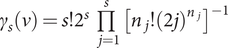 $ {\gamma}_s\left(\nu \right)=s!{2}^s\prod \limits_{j=1}^s{\left[{n}_j!{(2j)}^{n_j}\right]}^{-1} $
and Δ is a diagonal positive definite n × n matrix, R a symmetric n × n matrix and x an n × 1 vector given by
 $ \Delta ={\left({I}_n+2t\Lambda \right)}^{-\frac{1}{2}},\hskip1em R=\Delta {A}^{\ast}\Delta, \hskip1em \xi =\Delta {\mu}^{\ast }. $
Let y(z 1, z 2, …, zm) be a continuous, differentiable, separable polynomial of order n. Let x j be the vector of normally distributed polynomial coefficients of the variable zj in increasing order, that is, 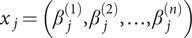 $ {x}_j=\left({\beta}_j^{(1)},{\beta}_j^{(2)},\dots, {\beta}_j^{(n)}\right) $. In that case, its mean μ = 0,
  $ \xi =\Delta {\mu}^{\ast }=0 $ and the covariance matrix Ω is a diagonal matrix with [r, r2, …, rn] on its diagonal.
Let A be the n × n matrix with  $ {A}_{i_1,{i}_2},{i}_1\ne {i}_2 $, is half the coefficient of
  $ {\beta}_j^{\left({i}_1\right)}{\beta}_j^{\left({i}_2\right)} $ and Ai,i is the coefficient of
  $ {\left({\beta}_j^{(i)}\right)}^2 $ in the numerator of Eq. (19). Let B be the n × n matrix with
  $ {B}_{i_1,{i}_2},{i}_1\ne {i}_2 $, is half the coefficient of
  $ {\beta}_j^{\left({i}_1\right)}{\beta}_j^{\left({i}_2\right)} $ and Bi,i is the coefficient of
  $ {\left({\beta}_j^{(i)}\right)}^2 $ in the denominator of Eq. (19). Then
 $ {\varepsilon}_{\sigma^2}=\frac{x^T Ax}{x^T Bx} $ and we can apply Theorem 1 for s = 1, giving the expected value and for s = 2, giving the variance of
  $ {\varepsilon}_{\sigma^2} $.
Theorem 2
Let y(z 1, z 2, …, zm) be a continuous, differentiable, separable polynomial of order n with polynomial coefficients that are mutually independent and normally distributed with zero mean and variances that decrease geometrically at rate r with the increasing of polynomial order, that is, 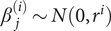 $ {\beta}_j^{(i)}\sim N\left(0,{r}^i\right) $.
Then the relative error  $ {\varepsilon}_{\sigma^2} $ of the quadrature method has mean
 $ \mathrm{E}\left[{\varepsilon}_{\sigma^2}\right]=m\underset{0}{\overset{\infty }{\int }}{\left(\prod \limits_{i=1}^n\frac{1}{\sqrt{1+2t{\lambda}_i}}\right)}^m\left(\sum \limits_{i=1}^n\frac{1}{\left(1+2t{\lambda}_i\right)}\sum \limits_{k=1}^n\sum \limits_{l=1}^n\sqrt{r^{k+l}}{P}_{k,i}{P}_{l,i}{A}_{k,l}\right) dt $
and variance
 $ \mathrm{E}{\left[{\varepsilon}_{\sigma^2}\right]}^2=m\underset{0}{\overset{\infty }{\int }}{\left(\prod \limits_{i=1}^n\frac{t}{\sqrt{1+2t{\lambda}_i}}\right)}^m\sum \limits_{i_1=1}^n\sum \limits_{i_2=1}^n\frac{X_{i_1{i}_2}}{\left(1+2t{\lambda}_{i_1}\right)\left(1+2t{\lambda}_{i_2}\right)} dt $
with
 $ {X}_{i_1{i}_2}=\sum \limits_{k_1=1}^n\sum \limits_{k_2=2}^n\sum \limits_{l_1=1}^n\sum \limits_{l_2=1}^n\sqrt{r^{k_1+{k}_2+{l}_1+{l}_2}}{P}_{i_1,{l}_1}{P}_{i_2,{l}_2}\left(2{P}_{i_2,{k}_1}{P}_{i_1,{k}_2}+{P}_{i_1,{k}_1}{P}_{i_2,{k}_2}\right){A}_{l_1,{k}_1}{A}_{l_2,{k}_2}. $
Here λ is a vector of eigenvalues and P is a matrix whose columns correspond to the eigenvectors of the matrix M = LTBL, with B the n × n matrix with  $ {B}_{i_1,{i}_2},{i}_1\ne {i}_2 $, is half the coefficient of
  $ {\beta}_j^{\left({i}_1\right)}{\beta}_j^{\left({i}_2\right)} $ and Bi,i is the coefficient of
  $ {\left({\beta}_j^{(i)}\right)}^2 $ in the denominator of Eq. (19) and L is a diagonal matrix with
 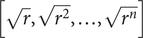 $ \left[\sqrt{r},\sqrt{r^2},\dots, \sqrt{r^n}\right] $ on its diagonal.
Proof
For s = 1, we have  $ \nu =\left[1\right] $ and
  $ {\gamma}_1\left(\left[1\right]\right)=1 $.
For s = 2, we have  $ {n}_1+2{n}_2=2 $, that is,
  $ \nu =\left[0,1\right] $ or
  $ \nu =\left[2,0\right] $, and
  $ {\gamma}_2\left(\left[0,1\right]\right)=2 $ and
  $ {\gamma}_2\left(\left[2,0\right]\right)=1 $.
Let L be the diagonal matrix with  $ \left[\sqrt{r},\sqrt{r^2},\dots, \sqrt{r^n}\right] $ on its diagonal, then Ω = LLT and let
 $ M={L}^T BL. $
Let P be an n × n matrix with the normalized eigenvectors of the matrix M as its columns, then PTP = In and
 $ \Lambda ={P}^T{L}^T BLP $
is the n × n diagonal matrix with the eigenvalues λ 1, …, λn of M on its diagonal. Let Δ be defined by
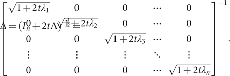 $ \Delta ={\left({I}_n+2t\Lambda \right)}^{-\frac{1}{2}}={\left[\begin{array}{ccccc}\sqrt{1+2t{\lambda}_1}& 0& 0& \cdots & 0\\ {}0& \sqrt{1+2t{\lambda}_2}& 0& \cdots & 0\\ {}0& 0& \sqrt{1+2t{\lambda}_3}& \cdots & 0\\ {}\vdots & \vdots & \vdots & \ddots & \vdots \\ {}0& 0& 0& \cdots & \sqrt{1+2t{\lambda}_n}\end{array}\right]}^{-1}. $
Then its determinant equals  $ \left|\Delta \right|=\prod \limits_{i=1}^n\frac{1}{\sqrt{1+2t{\lambda}_i}} $.
Let A* be defined by
$ {A}^{*}={P}^T{L}^T ALP $
Then R = Δ A* Δ equals
 $ R={\left({I}_n+2t\Lambda \right)}^{-1/2}{P}^T{L}^T ALP{\left({I}_n+2t\Lambda \right)}^{-1/2}. $
The elements of R equal
 $ {R}_{i_1,{i}_2}=\frac{1}{\sqrt{\left(1+2t{\lambda}_{i_1}\right)\left(1+2t{\lambda}_{i_2}\right)}}\sum \limits_{k=1}^n\sum \limits_{l=1}^n\sqrt{r^{k+l}}{P}_{i_1,k}{P}_{i_2,l}{A}_{l,k},{i}_1,{i}_2\in \left\{1,2,\dots, n\right\}. $
The diagonal elements of R 2 equal
 $ {R}_{i_1,{i}_1}^2=\sum \limits_{i_2=1}^n{R}_{i_2{i}_1}{R}_{i_1{i}_2},{i}_1\in \left\{1,2,\dots, n\right\}. $
Then
 $ {\displaystyle \begin{array}{c}\mathrm{E}\left[{\varepsilon}_{\sigma^2}\right]=\sum \limits_{j=1}^m\underset{0}{\overset{\infty }{\int }}\left|\Delta \right|\mathrm{tr}\, Rdt\hskip17pc \\ {}=m\underset{0}{\overset{\infty }{\int }}{\left(\prod \limits_{i=1}^n\frac{1}{\sqrt{1+2t{\lambda}_i}}\right)}^m\left(\sum \limits_{i=1}^n\frac{1}{\left(1+2t{\lambda}_i\right)}\sum \limits_{k=1}^n\sum \limits_{l=1}^n\sqrt{r^{k+l}}{P}_{k,i}{P}_{l,i}{A}_{k,l}\right) dt\end{array}} $
and
 $ {\displaystyle \begin{array}{c}\mathrm{E}{\left[{\varepsilon}_{\sigma^2}\right]}^2=\sum \limits_{j=1}^m2\underset{0}{\overset{\infty }{\int }}t\left|\Delta \right|\left(\mathrm{tr}\,{R}^2\right) dt+\underset{0}{\overset{\infty }{\int }}t\left|\Delta \right|{\left(\mathrm{tr}\,R\right)}^2 dt\hskip7.9pc \\ {}=\sum \limits_{j=1}^m\underset{0}{\overset{\infty }{\int }}t\left|\Delta \right|\left(2\,\mathrm{tr}\,{R}^2+{\left(\mathrm{tr}\,R\right)}^2\right) dt\hskip21.8em \\ {}=m\underset{0}{\overset{\infty }{\int }}{\left(\prod \limits_{i=1}^n\frac{t}{\sqrt{1+2t{\lambda}_i}}\right)}^m\left(2\sum \limits_{i_1=1}^n\sum \limits_{i_2=1}^n{R}_{i_2{i}_1}{R}_{i_1{i}_2}+{\left(\sum \limits_{i_1=1}^n{R}_{i_1{i}_1}\right)}^2\right) dt\\ {}=m\underset{0}{\overset{\infty }{\int }}{\left(\prod \limits_{i=1}^n\frac{t}{\sqrt{1+2t{\lambda}_i}}\right)}^m\sum \limits_{i_1=1}^n\sum \limits_{i_2=1}^n\left(2{R}_{i_2{i}_1}{R}_{i_1{i}_2}+{R}_{i_1{i}_1}{R}_{i_2{i}_2}\right) dt\hskip2.3pc \\ {}=m\underset{0}{\overset{\infty }{\int }}{\left(\prod \limits_{i=1}^n\frac{t}{\sqrt{1+2t{\lambda}_i}}\right)}^m\sum \limits_{i_1=1}^n\sum \limits_{i_2=1}^n\frac{X_{i_1{i}_2}}{\left(1+2t{\lambda}_{i_1}\right)\left(1+2t{\lambda}_{i_2}\right)} dt,\hskip2.4pc \end{array}} $
with
 $ {X}_{i_1{i}_2}=\sum \limits_{k_1=1}^n\sum \limits_{k_2=2}^n\sum \limits_{l_1=1}^n\sum \limits_{l_2=1}^n\sqrt{r^{k_1+{k}_2+{l}_1+{l}_2}}{P}_{i_1,{l}_1}{P}_{i_2,{l}_2}\left(2{P}_{i_2,{k}_1}{P}_{i_1,{k}_2}+{P}_{i_1,{k}_1}{P}_{i_2,{k}_2}\right){A}_{l_1,{k}_1}{A}_{l_2,{k}_2}. $
Assume that the function y(z) is a fifth-order separable polynomial and that the polynomial coefficients are normally distributed with zero mean and their variance that decreases geometrically at rate r with the increasing of polynomial order. For a fifth order polynomial, the numerator of Eq. (19) only consists of the term  $ 120{\left({\beta}_j^{(5)}\right)}^2 $, so
  $ {A}_{5,5}=120 $ and
  $ {A}_{i,j}=0 $ otherwise. Then, with Theorem 2, the relative error
  $ {\varepsilon}_{\sigma^2} $ of the quadrature method has mean
 $ \mathrm{E}\left[{\varepsilon}_{\sigma^2}\right]=-120{r}^5m\underset{0}{\overset{\infty }{\int }}{\left(\prod \limits_{i=1}^5\frac{1}{\sqrt{1+2t{\lambda}_i}}\right)}^m\left(\sum \limits_{i=1}^5\frac{P_{5,i}^2}{\left(1+2t{\lambda}_i\right)}\right) dt $
and variance
 $ \mathrm{E}{\left[{\varepsilon}_{\sigma^2}\right]}^2={120}^2{r}^{10}m\underset{0}{\overset{\infty }{\int }}{\left(\prod \limits_{i=1}^n\frac{t}{\sqrt{1+2t{\lambda}_i}}\right)}^m\sum \limits_{i_1=1}^n\sum \limits_{i_2=1}^n\frac{P_{i_1,5}{P}_{i_2,5}\left(2{P}_{i_2,5}{P}_{i_1,5}+{P}_{i_1,5}{P}_{i_2,5}\right)}{\left(1+2t{\lambda}_{i_1}\right)\left(1+2t{\lambda}_{i_2}\right)} dt. $
An interesting implication of Theorem 2 is that the expected value of error is nonzero for polynomials of order 5 and higher and therefore the quadrature-based method is biased in estimating the relative error  $ {\varepsilon}_{\sigma^2} $ for a fifth or higher order separable polynomial system.
Figure 4 presents results from Theorem 2 which can be used as a priori error estimates. Plotted are the expected value of error and the standard deviation of error for the quadrature-based method versus dimensionality m for a few different values of the parameter r. The plotted values were computed using Theorem 2 and confirmed via Monte Carlo simulation. The results are plotted over a range of values for the parameter  $ r $. It was shown empirically by Li & Frey (Reference Li and Frey2005) via a meta-analysis of published experiments that two-factor interactions are about 0.2 the size of the main effects on average across large populations of factorial experiments. This might suggest that 0.2 is a reasonable mean value for a prior probability of
  $ r $, but we also plotted results for somewhat higher and lower values of r.
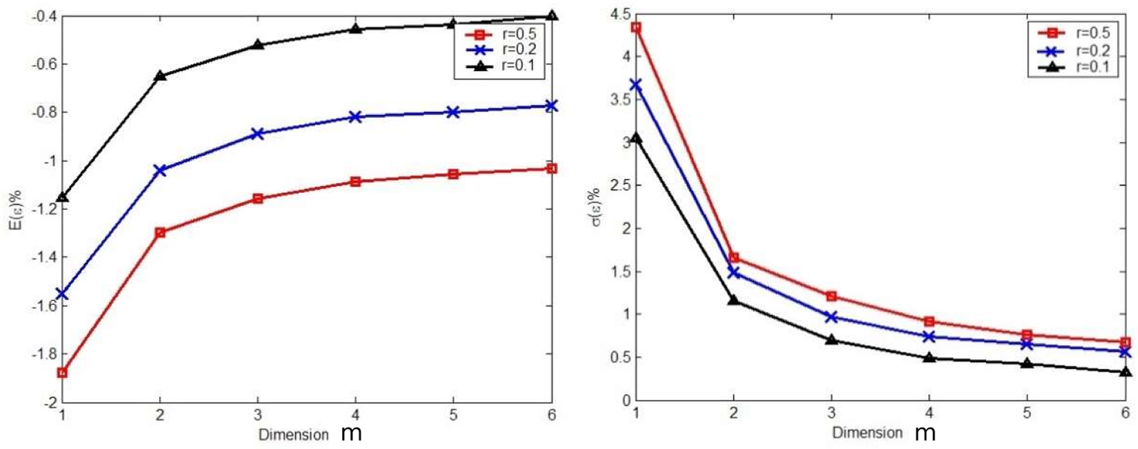
Figure 4. The scaling with dimensionality, m, of standard deviation of relative error, ε, for of the quadrature-based method when applied to separable functions.
The expected value of error for quadrature is strictly negative; therefore the estimates tend to be lower than the actual transmitted variance of the system, although the error can be positive in individual uses of the method. The mean error decreases and the dimensionality of the problem increases, but it does not converge asymptotically toward zero.
The first term in Eq. (17) is weighted by m while the second term is weighted by  $ {m}^2 $ and the denominators of both terms are raised to the power m. An interesting implication is that, if the function y is separable, the error variance of the method decreases monotonically and tends to zero in the limit as the number of noise factors, m, grows. This monotonicity and decay to zero hold for all values of the rate of decay r less than unity.
8. Comparative assessment via hierarchical probability models
The accuracy of the proposed method is determined by the relative size of single-factor effects and interactions and by the number of interactions. Thus, an error estimate might be based on a reasonable model of the size and probability of interactions. The hierarchical probability model was proposed by Chipman et al. (Reference Chipman, Hamada and Wu1997) as a means to more effectively derive response models from experiments with complex aliasing patterns. This model was fit to data from 46 full factorial engineering experiments (Li and Frey, Reference Li and Frey2005). The fitted model is useful for evaluating various techniques for robust design with computer experiments. Eqs. (20) through (27) comprise the model used here.
 $$ y=\sum \limits_{i=1}^n{\beta}_i{x}_i+\sum \limits_{j=1}^n\sum \limits_{\begin{array}{l}i=1\\ {}i\le j\end{array}}^n{\beta}_{ij}{x}_i{x}_j+\sum \limits_{k=1}^n\sum \limits_{\begin{array}{l}j=1\\ {}j\le k\end{array}}^n\sum \limits_{\begin{array}{l}i=1\\ {}i\le j\end{array}}^n{\beta}_{ij k}{x}_i{x}_j{x}_k $$
 $$ {x}_i\sim N\left(0,{\sigma}^2\right), $$
where σ = 10%.
 $$ f\left({\beta}_i\left|{\delta}_i\right.\right)=\left\{\begin{array}{c}N\left(0,1\right)\hskip0.36em \mathrm{if}\hskip0.36em {\delta}_{\mathrm{i}}=0\\ {}N\left(0,10\right)\hskip0.24em \mathrm{if}\hskip0.24em {\delta}_{\mathrm{i}}=1\end{array}\right. $$
 $$ f\left({\beta}_{ij}\left|{\delta}_{ij}\right.\right)=\left\{\begin{array}{c}N\left(0,1\right)\hskip0.36em \mathrm{if}\hskip0.36em {\delta}_{\mathrm{ij}}=0\\ {}N\left(0,10\right)\hskip0.24em \mathrm{if}\hskip0.24em {\delta}_{\mathrm{ij}}=1\end{array}\right. $$
 $$ f\left({\beta}_{ijk}\left|{\delta}_{ijk}\right.\right)=\left\{\begin{array}{c}N\left(0,1\right)\hskip0.36em \mathrm{if}\hskip0.36em {\delta}_{ijk}=0\\ {}N\left(0,10\right)\hskip0.24em \mathrm{if}\hskip0.24em {\delta}_{ijk}=1\end{array}\right. $$
 $$ \Pr \left({\delta}_i=1\right)=p $$
 $$ \Pr \left({\delta}_{ij}=1\left|{\delta}_i\right.,{\delta}_j\right)=\left\{\begin{array}{c}{p}_{00}\hskip0.36em \mathrm{if}\hskip0.36em {\delta}_{\mathrm{i}}+{\delta}_{\mathrm{j}}=0\\ {}{p}_{01}\hskip0.36em \mathrm{if}\hskip0.36em {\delta}_{\mathrm{i}}+{\delta}_{\mathrm{j}}=1\\ {}{p}_{11}\hskip0.36em \mathrm{if}\hskip0.36em {\delta}_{\mathrm{i}}+{\delta}_{\mathrm{j}}=2\end{array}\right. $$
 $$ \Pr \left({\delta}_{ijk}=1\left|{\delta}_i\right.,{\delta}_j,{\delta}_k\right)=\left\{\begin{array}{c}{p}_{000}\hskip0.36em \mathrm{if}\hskip0.36em {\delta}_{\mathrm{i}}+{\delta}_{\mathrm{j}}+{\delta}_{\mathrm{k}}=0\\ {}{p}_{001}\hskip0.36em \mathrm{if}\hskip0.36em {\delta}_{\mathrm{i}}+{\delta}_{\mathrm{j}}+{\delta}_{\mathrm{k}}=1\\ {}{p}_{011}\hskip0.36em \mathrm{if}\hskip0.36em {\delta}_{\mathrm{i}}+{\delta}_{\mathrm{j}}+{\delta}_{\mathrm{k}}=2\\ {}{p}_{111}\hskip0.36em \mathrm{if}\hskip0.36em {\delta}_{\mathrm{i}}+{\delta}_{\mathrm{j}}+{\delta}_{\mathrm{k}}=3\end{array}\right. $$
Eq. (20) expresses the assumption that the system response is a third order polynomial. Eq. (21) defines the input variations as random normal variates. We used a standard deviation of 10% because it represented a level of difficulty for the methods comparable to that found in most case studies we have found in the literature. Eqs. (22) through (24) assign probability distributions to the polynomial coefficients. Polynomial coefficients βι whose corresponding parameter δι = 1 have a larger probability of taking on a large positive or negative value. The values of the parameters δι are set in Eqs. (25) through (27). The values of the parameters in the model are taken from an empirical study of 113 full factorial experiments [16] and are p = 39%, p 00 = 0.48%, p 01 = 4.5%, p 11 = 33%, p 000 = 1.2%, p 001 = 3.5%, p 011 = 6.7% and p 111 = 15%.
For each integer  $ n\in \left[6,20\right] $, one thousand systems were sampled from the model (Eqs. (20 through (27)) The expected value and standard deviation of the response y was estimated in five ways:
(i) using the quadrature technique which required
 $ 4m+1 $ samples,
(ii) generating
$ 4m+1 $ samples via LHS and computing their mean and standard deviation,(iii) generating
$ 4m+1 $ samples via HSS and computing their mean and standard deviation,(iv) generating
$ 10\times \left(4m+1\right) $ samples via LHS and computing their mean and standard deviation and(v) generating
$ 10\times \left(4m+1\right) $ samples via HSS and computing their mean and standard deviation.


The exact solution was also determined using Eqs. (9 and (10), enabling the computation of the size of the error for each of the 1000 systems given each of the three methods. These data were used to estimate the cumulative probability versus error (Figure 4). In effect, this is a chart of confidence level versus error tolerance. The preference is for methods that lie higher on the chart since this indicates greater confidence that the given error tolerance will be satisfied than methods lower on the chart.
Figure 5 shows that the quadrature technique estimated the standard deviation within 5% for more than 95% of all systems sampled. Quadrature accomplished this with only  $ 4m+1 $ samples. HSS and LHS were unable to provide comparably good results with
  $ 4m+1 $ samples. However, given 10 times the resources, HSS achieved accuracy comparable to that of quadrature.

Figure 5. Cumulative probability versus error in estimating standard deviation for five different sampling procedures.
The model-based evaluation presented here assumes that the system response is a polynomial. This is a significant limitation. This approach can reveal the error due to the presence of interaction effects, but it cannot account for the errors due to departure of a system from a polynomial response approximation. For this reason, the case studies in the next section are an important additional check on the results.
9. Comparative assessment via case studies
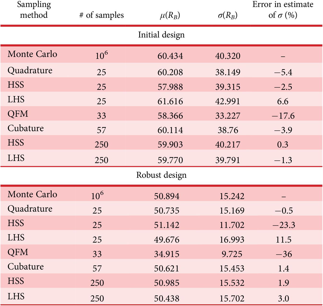
This section presents five computer simulations of engineering systems to which different methods for estimating transmitted variance are applied. One of the engineering systems, the LifeSat satellite, has two different responses making six responses total in the set of five systems. For each of the six responses, two designs within the parameter space are considered – an initial design and an alternative that exhibits lower transmitted variance (we will call this the “robust design”). As a result, there were 12 cases in total to which the sampling methods were applied.
9.1. Case 1: continuous-stirred tank reactor
The engineering system in this case is a continuous-stirred tank reactor (CSTR) which was used to demonstrate the advantages of HSS over LHS (McKay et al. Reference McKay, Beckman and Conover1979). The function of the CSTR system is to produce a chemical species B at a target production rate (RB) of 60 mol/min. Variations from the target (either above or below target) are undesirable. The CSTR system is comprised of a tank into which liquid flows at a volumetric flow rate (F) and initial temperature (Ti). The liquid contains two chemical species (A and B) with known initial concentrations (CAi and CBi). In addition to fluid, heat is added to the CSTR at a given rate (Q). Fluid flows from the CSTR at the same rate it enters but at different temperature (T) and with different concentrations of the species A and B (CA and CB). The system is governed by five equations.
 $$ Q= F\rho {C}_p\left(T-{T}_i\right)+V\left({r}_A{H}_{RA}+{r}_B{H}_{RB}\right), $$
 $$ {C}_A=\frac{C_{Ai}}{1+{k}_A^0{e}^{-{E}_A/ RT}\tau },\hskip7.2pc $$
 $$ {C}_B=\frac{C_{Bi}+{k}_A^0{e}^{-{E}_A/ RT}\tau {C}_A}{1+{k}_B^0{e}^{-{E}_B/ RT}\tau },\hskip5.5pc $$
 $$ -{r}_A={k}_A^0{e}^{-{E}_A/ RT}{C}_A,\hskip8.4pc $$
 $$ -{r}_B={k}_B^0{e}^{-{E}_B/ RT}{C}_B-{k}_A^0{e}^{-{E}_A/ RT}{C}_A,\hskip3.4pc $$
where the average residence time in the reactor is V/F and the realized production rate (RB) is rBV which has a desired target of 60 mol/min.
Table 1 provides a listing of physical constants, input and output variables. These values of physical constants and the input variables are taken directly from Kalagnanam & Diwekar (Reference Kalagnanam and Diwekar1997)) with the exception that the values of T and Ti were swapped to correct for a typographical error in the previous paper pointed out to us by its authors. Following the example of Kalagnam and Diwekar’s paper, we assume that all the input variables are independent and normally distributed with a standard deviation of 10% of the mean. We considered two different “designs” (i.e., nominal values for the input variables) described in Kalagnam and Diwekar’s paper – one was an initial design and the other was an optimized robust design with greatly reduced variance in the response RB.
Table 1. Parameters and their values in the continuous-stirred tank reactor case study

To check that the model was correctly implemented, the results at both points were reproduced by Monte Carlo simulations with 106 trials each. Kalagnam and Diwekar found a transmitted variance in the initial design of 1638 (mol/min)2 and we computed a transmitted variance of 1625.7 ± 1.5 (mol/min)2. There was also a small discrepancy in the transmitted variance of the robust design – the published value was 232 (mol/min)2 and we computed 232.3 ± 0.4 (mol/min)2. The discrepancy between our results and the previously published results is small (less than 0.2%) and likely due to differences in implementation of the solver for the system of equations.
Monte Carlo simulations were run using 106 samples to estimate the true standard deviation of the response of the CSTR due to the six noise factors. Then, six different methods were used to estimate the standard deviation of the response: (1) the quadrature technique using 25 samples; (2) HSS using 25 samples; (3) LHS using 25 samples; (4) QFM which required 33 samples; (5) HSS using 250 samples and (6) LHS using 250 samples.
Table 2 presents the results. The error of the quadrature technique as applied to the CSTR was about 5% for the initial design and improved substantially when the design was made more robust. Given that there were nine randomly varying inputs, Theorem 2 suggested that the mean error would be about –0.5% and the standard deviation of error would be about 0.5 to 1%. These results are consistent with Theorem 2 at the robust set point, but the response to noise was unexpectedly challenging for the initial set point. HSS with 25 samples outperformed quadrature at the initial design, but then performed very poorly at the robust design. Cubature had slightly lower error than quadrature at the initial design, but quadrature performed much better than cubature at the robust design set point and also required about half as many function evaluations.
Table 2. Comparing the accuracy of sampling methods as applied to the continuous-stirred tank reactor
9.2. Case 2: LifeSat satellite
The engineering system in this case is a LifeSat satellite which was used to demonstrate the benefits of the Taguchi method (Mistree et al. Reference Mistree, Lautenschlager, Erikstad and Allen1993). The objective is to select a few key initial conditions at the start of a satellite de-orbit maneuver in order to have the satellite land near a specified target while minimizing the maximum acceleration and dynamic pressure during the de-orbit trajectory. The satellite itself is modeled as a point mass subject to gravitational, drag, and lift forces. The de-orbit sequence is as follows. First, the satellite is subjected to a prescribed thrust to set it on a de-orbit path. The initial state of the satellite after this thrust is described by a three-dimensional position and a velocity vector. Next, the satellite proceeds through a freefall stage whereby it experiences the effects of gravity drag and lift forces until it contacts the earth’s surface. The states of importance in the calculation of this trajectory are the landing position and a measure representative of the maximum force that the satellite experiences during free fall. The system is governed by three equations.
 $$ {\boldsymbol{F}}_{tot}=-m\left(\mu /{R}^2\right){\boldsymbol{e}}_R+\frac{1}{2}\rho {v}_r^2{A}_{ref}{c}_d{\boldsymbol{e}}_d, $$
 $$ \rho \hskip1.5pt \approx \hskip1.5pt {\rho}_0\cdot \exp \left[-\left(h-{h}_o\right)/{h}_s\right], $$
 $$ \mu = {gR}_0^2. $$
Table 3 provides a listing of physical constants and nine dispersed vehicle and environmental parameters (Mistree et al. Reference Mistree, Lautenschlager, Erikstad and Allen1993). We considered two different designs both described in the published case – one was an initial design and the other was an optimized robust design with greatly reduced variance in the landing coordinate.
Table 3. Parameters and their values in the LifeSat case study

In order to validate the simulation code, a verification study was performed. Mistree et al. (Reference Mistree, Lautenschlager, Erikstad and Allen1993) found the landing position of –106.65° longitude and 33.71° latitude. We obtained –106.65° longitude and 33.69° latitude.
Monte Carlo simulations were run using 104 samples to estimate the true standard deviation of both landing longitude and latitude due to the nine noise factors. Then, six different methods were used to estimate the standard deviation of the response: (1) quadrature (Eqs. (4)–(6)) using 4n + 1 or 37 samples; (2) HSS using 37 samples; (3) LHS using 37 samples; (4) QFM which required 33 samples; (5) HSS using 370 samples; and (6) LHS using 370 samples.
Tables 4 and 5 present the results. The error of the quadrature technique as applied to the LifeSat satellite was less than 2% for the initial design and robust design. Given that there were nine randomly varying inputs, Theorem 2 suggested that the mean error would be about –0.5% and the standard deviation of error would be about 0.5% to 1%. These results are generally consistent with Theorem 2 at both the robust set point and the initial set point. Quadrature outperformed HSS, LHS, and QFM with similar samples at both the initial design and the robust design. Cubature required three times as many function evaluations and yet performed less well than quadrature.
Table 4. Comparing the accuracy of sampling methods as applied to the LifeSat satellite (longitude)

Table 5. Comparing the accuracy of sampling methods as applied to the LifeSat satellite (latitude)

9.3. Case #3: I Beam
The engineering system in this case is an I beam which was used to demonstrate the advantages of dimension reduction integration in uncertainty analysis (Huang & Du Reference Huang and Du2005). The parameters in the model are depicted graphically in Figure 6.

Figure 6. Parameters of an I-beam (adapted from Huang & Du (Reference Huang and Du2005)).
The system is governed by the following three equations
 $$ Y=g(X)={\sigma}_{\mathrm{max}}-S, $$
 $$ {\sigma}_{\mathrm{max}}=\frac{Pa\left(L-a\right)d}{2L\cdot I}, $$
 $$ I=\frac{b_f{d}^3-\left({b}_f-{t}_w\right){\left(d-2{t}_f\right)}^3}{12}, $$
Table 6 provides a listing of eight random variables which are taken directly from the published case study (Huang & Du Reference Huang and Du2005). We considered two different designs – one was an initial design from the published case and the other was an optimized robust design proposed here with greatly reduced variance in the output performance.
Table 6. Parameters and their values in the I beam case study

To check that the model was correctly implemented, the results at both points were reproduced by Monte Carlo simulations with 106 trials each. Huang & Du (Reference Huang and Du2005) found the first and second estimated moments about zero using 106 samples. The previously published value of the transmitted variance was 3.2137 × 10⁸. We computed the transmitted variance of 3.2048 × 10⁸. The discrepancy between our results and the previously published results is small (less than 0.3%).
Monte Carlo simulations were run using 106 samples to estimate the true standard deviation of the output performance due to the eight noise factors. Then, six different methods were used to estimate the standard deviation of the response: (1) quadrature (Eqs. (3) and (4)) using 4n + 1 or 33 samples; (2) HSS using 33 samples; (3) LHS using 33 samples; (4) QFM which required 33 samples; (5) HSS using 330 samples and 6) LHS using 330 samples.
Table 7 presents the results of the case study. The accuracy of the quadrature technique as applied to the I-beam was excellent and generally as expected according to Theorem 2. The error was less than 1% and improved slightly as the design was made more robust. This level of accuracy was superior to any method using a comparable number of samples. However, if HSS was afforded 10 times the number of samples as quadrature, it could also provide excellent accuracy. Cubature required more than twice the function evaluations and performed better at the initial set point but worse than quadrature at the robust set point.
Table 7. Comparing the accuracy of sampling methods as applied to the I beam

9.4. Case #4: 10-bar truss
The engineering system in this case is a linear-elastic 10-bar truss structure which was used to demonstrate the accuracy and efficiency of the univariate approximation method in higher-order reliability analysis (Rahman & Wei Reference Rahman and Wei2006). Two concentrated forces are applied at nodes 2 and 3 of the structure as indicated in Figure 7. The maximum displacement occurs at node 3 which is taken as the performance function of interest. Although the components of the truss behave linearly with applied load, the displacements of the structure are large enough to bring about significantly nonlinear behavior of the structure.
Figure 7. Parameters of a 10-bar truss (from Rahman & Wei (Reference Rahman and Wei2006)).
Table 8 provides a listing of physical constants and 10 random variables which are taken from the published case (Rahman & Wei Reference Rahman and Wei2006). We considered two different “designs” – one was an initial design given in the published case and the other was an optimized robust design proposed here with greatly reduced variance in the output performance.
Table 8. Parameters and their values in the 10-bar truss case study

To check that the model was correctly implemented, the failure probability of the 10-bar truss structure was reproduced by Monte Carlo simulations with 106 trials. Rahman found a failure probability of 0.1394 using 106 samples (Rahman & Wei Reference Rahman and Wei2006) and we computed 0.1392 using 106 samples. The discrepancy between our results and the previously published results are small (less than 0.2%).
Monte Carlo simulations were run using 106 samples to estimate the true standard deviation of the output performance due to the 10 noise factors. Then, six different methods were used to estimate the standard deviation of the response: (1) quadrature (Eqs. (4)–(6)) using 4n + 1 or 41 samples; (2) HSS using 41 samples; (3) LHS using 41 samples; (4) QFM which required 33 samples; (5) HSS using 410 samples; and (6) LHS using 410 samples.
Table 9 presents the results. The error of the quadrature technique as applied to the 10-bar truss was around 3% for both the initial design and the robust design. Given that there were eight randomly varying inputs, Theorem 2 suggested that the mean error would be about -0.5% and the standard deviation of error would be about 0.5 to 1%. These results suggest that the 10-bar truss was somewhat challenging case for quadrature. LHS and HSS outperform quadrature if they are afforded 10 times number of samples but are substantially less reliable if they have to use the same number of samples as quadrature. Note that in this case study, the standard deviation of noise factor is 20% of the mean whereas in the model-based evaluation of Section 4, the standard deviation of noise factor is 10% of the mean. Cubature required more than three times as many function evaluations and had similar performance as quadrature.
Table 9. Comparing the accuracy of sampling methods as applied to the 10-bar truss

9.5. Case 5: operational amplifier
The engineering system in this case is an operational amplifier (op amp) which was used by to demonstrate the use of orthogonal arrays for robust design with computer simulations (Phadke Reference Phadke1989). The circuit is presented in Figure 7. The op amp is to be manufactured on a single board using 15 circuit elements whose parameters are to be chosen so that the offset voltage of the circuit is consistent despite manufacturing variations. There are 21 noise factors which affect the offset voltage (20 characterizing the circuit elements and one for the operating temperature) as shown in Table 10. Following the example of Phadke, we modeled some of the noise factors as correlated and some as independent. Phadke defined sliding levels to use in an L36 orthogonal outer array. We calculated the covariance matrix for the noise exhibited in the L36 array, and then ran various sampling schemes assuming the same covariance. Phadke also defined some noise factors as lognormally distributed. We adapted different sampling methods by transforming those input variables and then treating the transformed inputs as normally distributed variates. We considered two different designs, an initial design and a robust design as described in Table 10 (Phadke Reference Phadke1989).
Table 10. Noise factors in the op amp case study, means and standard deviations

We developed a simulation of the op amp circuit based on an Ebers-Moll model of the transistors. To check that the model was correctly implemented, the results were checked against Phadke’s published figures for the L36 outer array. Once the simulation was verified, we tested sampling techniques on it.
Monte Carlo simulations were run using 3 × 10⁴ samples to estimate the true standard deviation of the response of the op amp due to the 21 noise factors. Then, four different methods were used to estimate the standard deviation of the offset voltage: (1) the quadrature technique (Eqs. (3)–(5)) using 2m + 1 or 43 samples; (2) HSS using 43 samples; (3) LHS using 43 samples; (4) HSS using 430 samples; and (5) LHS using 430 samples.
Table 11 presents the results of the case study. The accuracy of the quadrature technique as applied to the op amp was excellent beginning at less than 1% error and improving slightly as the design was made more robust. Given that there were 19 randomly varying inputs, Theorem 2 suggested that the accuracy would be improved compared to the other cases which is what we observed. The level of accuracy attained by quadrature was superior to any method using a comparable number of samples. However, if HSS was afforded 10 times the number of samples as quadrature, it could also provide excellent accuracy. Unlike the other four systems simulated, QFM was not run on the op amp. The method could not be scaled to accommodate the large number of noise factors. Instead an L36 orthogonal array is presented as a basis of comparison. The L36 provided good results for this system, but not as good as the quadrature technique. The cubature method required more than 10 times the function evaluations and performed less well than quadrature.
Table 11. Comparing the accuracy of sampling methods as applied to the operational amplifier

9.6. All the case studies as a set
The set of case studies presented here can be studied as a set. There were five engineering systems and six different responses. For each response, there were an initial and a robust design making 12 case studies in total. Given the accuracy of each method applied across all the cases, it is possible to construct an empirical cdf of its accuracy. These are presented in Figure 8 with the model-based cdf for the 4m + 1 quadrature technique as previously presented in Figure 5.

Figure 8. Empirical cumulative density functions based on the set of case studies. The model-based cumulative density functions of the 4m + 1 quadrature technique is provided for comparison.
A principal observation is that, for the 4m + 1 quadrature technique, the empirical cdf largely matches the model-based cdf. In the range of 3%–5% accuracy, the empirical cdf indicated a somewhat lower probability than the model-based cdf, but this deviation is within the 95% confidence range predicted by the model when only 12 samples are used to construct a cdf (the 95% range is not depicted since Figure 6 is already very dense). Note that the case studies make no assumption of polynomial response behavior. Therefore we submit that the model-based approach to evaluating the accuracy of the sampling methods has passed a stringent test.
Another important set of conclusions arise from comparing the empirical cdfs for the different methods. As in the model-based evaluation, quadrature substantially outperforms the previously available methods when they employ a comparable number of simulations. For the case studies, it appears that if 10 times the number of simulations can be run, then quadrature provides slightly better results.
Also, note that in four out of five case studies, the accuracy of quadrature is better for the robust design than for the initial design. It is not yet clear that this phenomenon is reliable, but it would be useful if it were. As the outer optimization loop begins to hone in on promising design candidates, the ability to make finer distinctions becomes more valuable.
Overall, the case studies as a set are consistent with the principal claims from the model-based evaluation. The quadrature technique enables a 10-fold reduction in the number of computational simulations needed for robust design while providing reasonable accuracy. In addition, the accuracy of the method usually improves as the design is made more robust which should be advantageous when the method is used as an inner loop of a robustness optimization procedure.
10. Conclusions
This paper provides an alternative tool for practitioners to efficiently estimate transmitted variance as part of Robust Parameter Design. This tool is based on Hermite–Gaussian quadrature which, by exploiting the property of hierarchy and compromising slightly on accuracy and bias, greatly reduces the number of samples needed and scales linearly with the number of variables. This paper provides an analysis of the accuracy of the estimated transmitted variance using the quadrature-based method for separable polynomial response systems. It is verified that the method gives exact transmitted variance if the response is up to a fourth-order separable polynomial response. Closed form expressions were derived for the error as well as for the statistical properties of the error (i.e., the mean and variance of error).
The advantages of the quadrature-based method were demonstrated by means of hierarchical probability models and a set of case studies. For typical populations of problems, it is shown that the method has good accuracy, providing less than 5% error in 90% of the applications. The proposed method provides much better accuracy than LHS or HSS, assuming these techniques are also restricted to using 4m + 1 samples. Only if Hammersley Sequence Sampling is afforded at least 10 times the number of samples, can it provide approximately the same degree of accuracy as the quadrature technique.
The limitations of the quadrature-based method should be emphasized. The theorems and model-based evaluations in this paper are predicated on the assumption that the noise factors are all normally distributed and probabilistically independent. To accommodate correlated noise factors, a linear transformation can be applied to the noise variables to create a set of uncorrelated noise factors before applying the equations in this paper. This approach was used in the op-amp case study and it was effective in that application. More generally, the Mahalanobis transformation will serve to create a set of independent random variables from a set of normally distributed, correlated random variables (Härdle & Simar Reference Härdle and Simar2007). However, it should be noted that the transformed, uncorrelated noise factors will not always be probabilistically independent except under particular assumptions, for example, when the noise factors are all normally distributed. We have not yet determined how well the proposed quadrature method will work on correlated variables that depart significantly from a normal distribution.
It’s an interesting fact that the quadrature-based method had improved accuracy at the robust set point (as compared to the initial design) in most of the case studies. This potential regularity has yet to be verified and would require more case studies to develop confidence in its existence and reliability. However, it seems reasonable that as a system becomes more robust to a set of noise factors, its response to noise also becomes more nearly separable. For a set point to exhibit substantial robustness as compared to other set points, the response surface (to noise factors, not control factors) has to be relatively flat, relatively smooth, and nearly devoid of salient features. It stands to reason that response surfaces matching this description might also be separable in their response to noise. If so, this would be an auspicious development for the quadrature method. As the robust design process searches for robust set points, it also improves the degree to which the assumptions needed for quadrature are satisfied.
It is hoped that the advantages of the quadrature-based method will prove helpful for engineering designers facing the demands of real-world pressures such as time and resource limitations. The proposed quadrature-based method adds value to the practitioner’s toolbox. When practical engineering problems have less separability and smaller numbers of input variables, a cubature method might be a reasonable choice. A cubature method such as proposed by Lu & Darmofal (Reference Lu and Darmofal2005) will afford advantages when there are practically significant noise by noise interactions. The meta-model based approach proposed by Tan & Wu (Reference Tan and Wu2012) may offer advantages when a Gaussian process model can closely fit the true underlying response of the engineering system. However, when practitioners face engineering problems with larger numbers of input variables, the quadrature-based method can estimate the transmitted variance efficiently and accurately as compared to other approaches. The developments in this paper also provide a priori error estimates that appear to be reliable, so the method can be applied with confidence.


 Open access