


Impact Statement
Real-time budgets arise in numerous settings, our focus is on the deployment of Monte Carlo methods on large-scale distributed computing systems, using real-time budgets to ensure the simultaneous readiness of multiple processors for collective communication, minimizing wasteful idle times that precedes it. A conceptual solution is found in the anytime algorithm. Our first major contribution is a framework for converting any existing Monte Carlo algorithm into an anytime Monte Carlo algorithm, by running multiple Markov chains in a particular manner. The second major contribution is a demonstration on a large-scale Monte Carlo implementation executing billions of samples distributed across a cluster of 128 graphics processing units. Our anytime algorithm demonstrably reduces idleness and provides control over the total compute budget.
1. Introduction
Real-time budgets arise in embedded systems, fault-tolerant computing, energy-constrained computing, distributed computing and, potentially, management of cloud computing expenses and the fair computational comparison of methods. Here, we are particularly interested in the development of Monte Carlo algorithms to observe such budgets, as well as the statistical properties—and limitations—of these algorithms. While the approach has broader applications, the pressing motivation in this work is the deployment of Monte Carlo methods on large-scale distributed computing systems, using real-time budgets to ensure the simultaneous readiness of multiple processors for collective communication, minimizing the idle wait time that typically precedes it.
A conceptual solution is found in the anytime algorithm. An anytime algorithm maintains a numerical result at all times, and will improve upon this result if afforded extra time. When interrupted, it can always return the current result. Consider, for example, a greedy optimization algorithm: its initial result is little more than a guess, but at each step it improves upon that result according to some objective function. If interrupted, it may not return the optimal result, but it should have improved on the initial guess. A conventional Markov chain Monte Carlo (MCMC) algorithm, however, is not anytime if we are interested in the final state of the Markov chain at some interruption time: as will be shown, the distribution of this state is length-biased by compute time, and this bias does not reduce when the algorithm is afforded additional time.
MCMC algorithms are typically run for some long time and, after removing an initial burn-in period, the expectations of some functionals of interest are estimated from the remainder of the chain. The prescription of a real-time budget, t, introduces an additional bias in these estimates, as the number of simulations that will have been completed is a random variable,  $ N(t). $ This bias diminishes in $ t $, and for long-run Markov chains may be rendered negligible. In motivating this work, however, we have in mind situations where the final state of the chain is most important, rather than averages over all states. The bias in the final state does not diminish in $ t $. Examples where this may be important include (a) sequential Monte Carlo (SMC), where, after resampling, a small number of local MCMC moves are performed on each particle before the next resampling step and (b) parallel tempering, where, after swapping between chains, a number of local MCMC moves are performed on each chain before the next swap. In a distributed computing setting, the resampling step of SMC, and the swap step of parallel tempering, require the synchronization of multiple processes, such that all processors must idle until the slowest completes. By fixing a real-time budget for local MCMC moves, we can reduce this idle time and eliminate the bottleneck, but must ensure that the length bias imposed by the real-time budget is negligible, if not eliminated entirely. In a companion paper (d’Avigneau et al., Reference d’Avigneau, Singh and Murray2020), we also develop this idea for parallel tempering-based MCMC.
The compute time of a Markov chain depends on exogenous factors such as processor hardware, memory bandwidth, I/O load, network traffic, and other jobs contesting the same processor. But, importantly, it may also depend on the states of the Markov chain. Consider (a) inference for a mixture model where one parameter gives the number of components, and where the time taken to evaluate the likelihood of a dataset is proportional to the number of components; (b) a differential model that is numerically integrated forward in time with an adaptive time step, where the number of steps required across any given interval is influenced by parameters; (c) a complex posterior distribution simulated using a pseudomarginal method (Andrieu and Roberts, Reference Andrieu and Roberts2009), where the number of samples required to marginalize latent variables depends on the parameters; (d) a model requiring approximate Bayesian computation with a rejection sampling mechanism, where the acceptance rate is higher for parameters with higher likelihood, and so the compute time lower, and vice versa. Even in simple cases, there may be a hidden dependency. Consider, for example, a Metropolis–Hastings sampler where there is some seemingly innocuous book-keeping code, such as for output, to be run when a proposal is accepted, but not when a proposal is rejected. States from which the proposal is more likely to accept then have longer expected hold time due to this book-keeping code. In general, we should assume that there is indeed a dependency, and assess whether the resulting bias is appreciable.
The first major contribution of the present work is a framework for converting any existing Monte Carlo algorithm into an anytime Monte Carlo algorithm, by running multiple Markov chains in a particular manner. The framework can be applied in numerous contexts where real-time considerations might be beneficial. The second major contribution is an application in one such context: an SMC $ {}^2 $ algorithm deployed on a large-scale distributed computing system. An anytime treatment is applied to the MCMC moves steps that precede resampling, which requires synchronization between processors, and can be a bottleneck in distributed deployment of the algorithm. The real-time budget reduces wait time at synchronization, relieves the resampling bottleneck, provides direct control over the compute budget for the most expensive part of the computation, and in doing so provides indirect control over the total compute budget.
Anytime Monte Carlo algorithms have recently garnered some interest. Paige et al. (Reference Paige, Wood, Doucet and Teh2014) propose an anytime SMC algorithm called the particle cascade. This transforms the structure of conventional SMC by running particles to completion one by one with the sufficient statistics of preceding particles used to make birth–death decisions in place of the usual resampling step. To circumvent the sort of real-time pitfalls discussed in this work, a random schedule of work units is used. This requires a central scheduler, so it is not immediately obvious how the particle cascade might be distributed. In contrast, we propose, in this work, an SMC algorithm with the conventional structure, but including parameter estimation as in SMC $ {}^2 $ (Chopin et al., Reference Chopin, Jacob and Papaspiliopoulos2013), and an anytime treatment of the move step. This facilitates distributed implementation, but provides only indirect control over the total compute budget.
The construction of Monte Carlo estimators under real-time budgets has been considered before. Heidelberger (Reference Heidelberger1988), Glynn and Heidelberger (Reference Glynn and Heidelberger1990), and Glynn and Heidelberger (Reference Glynn and Heidelberger1991) suggest a number of estimators for the mean of a random variable after performing independent and identically distributed (iid) simulation for some prescribed length of real time. Bias and variance results are established for each. The validity of their results relies on the exchangeability of simulations conditioned on their number, and does not extend to MCMC algorithms except for the special cases of regenerative Markov chains and perfect simulation. The present work establishes results for MCMC algorithms (for which, of course, iid sampling is a special case) albeit for a different problem definition.
A number of other recent works are relevant. Recent papers have considered the distributed implementation of Gibbs sampling and the implications of asynchronous updates in this context, which involves real time considerations (Terenin et al., Reference Terenin, Simpson and Draper2015; De Sa et al., Reference De Sa, Olukotun and Ré2016). As mentioned above, optimization algorithms already exhibit anytime behavior and it is natural to consider whether they might be leveraged to develop anytime Monte Carlo algorithms, perhaps in a manner similar to the weighted likelihood bootstrap (Newton and Raftery, Reference Newton and Raftery1994). Meeds and Welling (Reference Meeds, Welling, Cortes, Lawrence, Lee, Sugiyama and Garnett2015) suggest an approach along this vein for approximate Bayesian computation. Beyond Monte Carlo, other methods for probabilistic inference might be considered in an anytime setting. Embedded systems, with organic real-time constraints, yield natural examples (e.g., Ramos and Cozman, Reference Ramos and Cozman2005).
The remainder of the paper is structured as follows. Section 2 formalizes the problem and the framework of a proposed solution; proofs are deferred to Appendix 7 in Supplementary Material. Section 3 uses the framework to establish SMC algorithms with anytime moves, among them an algorithm suitable for large-scale distributed computing. Section 4 validates the framework on a simple toy problem, and demonstrates the SMC algorithms on a large-scale distributed computing case study. Section 5 discusses some of the finer points of the results, before Section 6 concludes.
2. Framework
Let  $ {\left({X}_n\right)}_{n=0}^{\infty } $ be a Markov chain with initial state $ {X}_0 $, evolving on a space $ \unicode{x1D54F} $, with transition kernel $ {X}_n\hskip.2em \mid \hskip.2em {x}_{n-1}\sim \kappa \left(\mathrm{d}x\hskip.2em |\hskip0.2em {x}_{n-1}\right) $ and target (invariant) distribution $ \pi \left(\mathrm{d}x\right) $. We do not assume that $ \kappa $ has a density, for example, it may be a Metropolis—Hastings kernel. (In contrast the notation for a probability density would be $ \kappa \left(x\hskip0.2em |\hskip0.2em {x}_{n-1}\right). $) A computer processor takes some random and positive real time $ {H}_{n-1} $ to complete the computations necessary to transition from $ {X}_{n-1} $ to $ {X}_n $ via $ \kappa $. Let $ {H}_{n-1}\hskip.2em \mid \hskip.2em {x}_{n-1}\sim \tau \left(\mathrm{d}h\hskip.2em |\hskip.2em {x}_{n-1}\right) $ for some probability distribution $ \tau $. The cumulative distribution function (cdf) corresponding to $ \tau $ is denoted $ {F}_{\tau}\left(h\hskip.2em |\hskip.2em {x}_{n-1}\right) $, and its survival function $ {\overline{F}}_{\tau}\left(h\hskip.2em |\hskip.2em {x}_{n-1}\right)=1-{F}_{\tau}\left(h\hskip.2em |\hskip.2em {x}_{n-1}\right) $. We assume (a) that $ H>\epsilon >0 $ for some minimal time $ \epsilon $, (b) that $ {\sup}_{x\in \unicode{x1D54F}}{\unicode{x1D53C}}_{\tau}\left[H\hskip.2em |\hskip.2em x\right]<\infty $, and (c) that $ \tau $ is homogeneous in time.
The distribution  $ \tau $ captures the dependency of hold time on the current state of the Markov chain, as well as on exogenous factors such as contesting jobs that run on the same processor, memory management, I/O, network latency, and so on. The first two assumptions seem reasonable: on a computer processor, a computation must take at least one clock cycle, justifying a lower bound on $ H $, and be expected to complete, justifying finite expectation. The third assumption, of homogeneity, is more restrictive. Exogenous factors may produce transient effects, such as a contesting process that begins part way through the computation of interest. We discuss the relaxation of this assumption—as future work—in Section 5.
Besides these assumptions, no particular form is imposed on  $ \tau $. Importantly, we do not assume that $ \tau $ is memoryless. In general, nothing is known about $ \tau $ except how to simulate it, precisely by recording the length of time $ {H}_{n-1} $ taken to simulate $ {X}_n\hskip0.2em \mid \hskip0.2em {x}_{n-1}\sim \kappa \left(\mathrm{d}x\hskip0.2em |\hskip0.2em {x}_{n-1}\right) $. In this sense, there exists a joint kernel $ \kappa \left(\mathrm{d}{x}_n,\mathrm{d}{h}_{n-1}\hskip0.2em |\hskip0.2em {x}_{n-1}\right)=\kappa \left(\mathrm{d}{x}_n|{h}_{n-1},{x}_{n-1}\right)\tau \left(\mathrm{d}{h}_{n-1}|{x}_{n-1}\right) $ for which the original kernel $ \kappa $ is the marginal over all possible hold times $ {H}_{n-1} $ in transit from $ {X}_{n-1} $ to $ {X}_n $:
 $$ \kappa \left(\mathrm{d}x\hskip.2em |\hskip.2em {x}_{n-1}\right)={\int}_0^{\infty}\kappa \left(\mathrm{d}x\hskip.2em |\hskip.2em {x}_{n-1},{h}_{n-1}\right)\tau \left(\mathrm{d}\hskip.2em {h}_{n-1}|\hskip.2em {x}_{n-1}\right). $$
We now construct a real-time semi-Markov jump process to describe the progress of the computation in real time. The states of the process are given by the sequence  $ {\left({X}_n\right)}_{n=0}^{\infty } $, with associated hold times $ {\left({H}_n\right)}_{n=0}^{\infty } $. Define the arrival time of the $ n $th state $ {X}_n $ as
 $$ {A}_n\hskip.2em := \hskip.2em \sum \limits_{i=0}^{n-1}{H}_i, $$
for all  $ n\hskip0.3em \ge \hskip0.2em 1 $, and $ {a}_0=0 $, and a process counting the number of arrivals by time $ t $ as
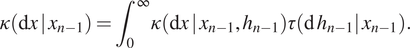
 $$ N(t)\hskip.2em := \hskip.2em \max \left\{n:{A}_n\hskip.2em \le \hskip.2em t\right\}. $$
Figure 1 illustrates a realization of the process.
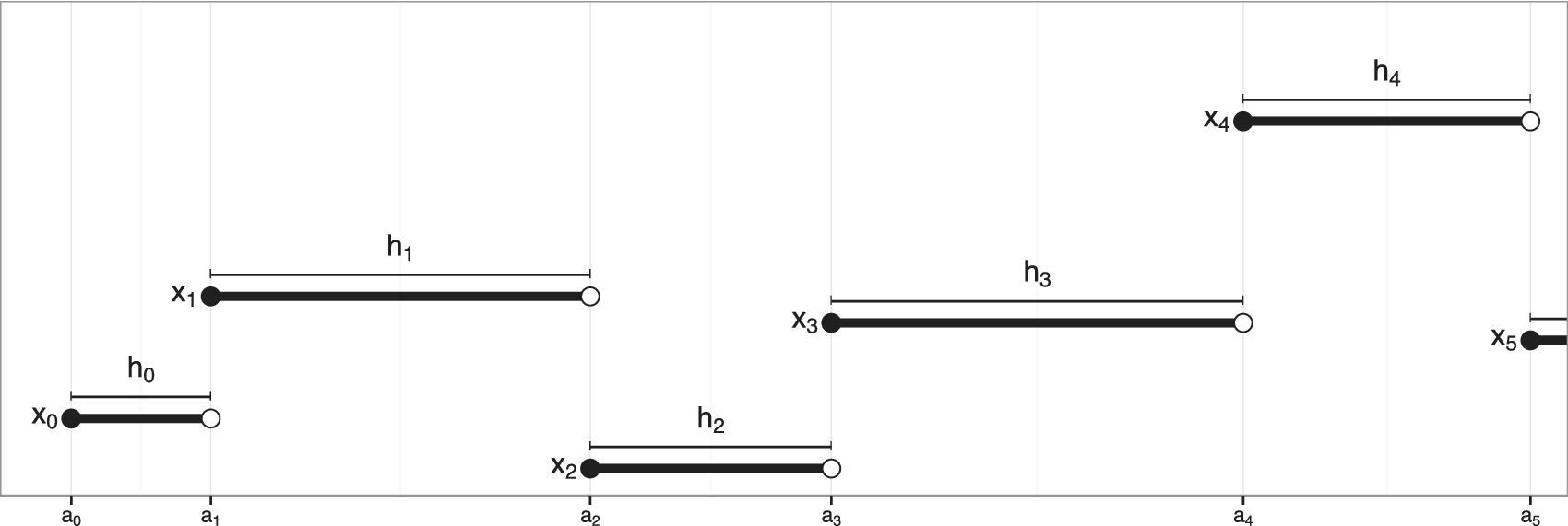
Figure 1. A realization of a Markov chain  $ {\left({X}_n\right)}_{n=0}^{\infty } $ in real time, with hold times $ {\left({H}_n\right)}_{n=0}^{\infty } $ and arrival times $ {\left({A}_n\right)}_{n=0}^{\infty } $.
Now, construct a continuous-time Markov jump process to chart the progress of the simulation in real time. Let  $ X(t)\hskip.2em := \hskip.2em {X}_{N(t)} $ (the interpolated process in Figure 1) and define the lag time elapsed since the last jump as $ L(t)\hskip.2em := \hskip.2em t-{A}_{N(t)} $. Then $ \left(X,\hskip.2em L\right)(t) $ is a Markov jump process.
The process  $ \left(X,\hskip.2em L\right)(t) $ is readily manipulated to establish the following properties. Proofs are given in Appendix A in Supplementary Material.
Proposition 1. The stationary distribution of the Markov jump process  $ \left(X,\hskip.2em L\right)(t) $ is
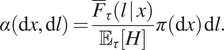 $$ \alpha \left(\mathrm{d}x,\mathrm{d}l\right)=\frac{{\overline{F}}_{\tau}\left(l\hskip.2em |\hskip0.2em x\right)}{{\unicode{x1D53C}}_{\tau}\left[H\right]}\pi \left(\mathrm{d}x\right)\hskip0.1em \mathrm{d}l. $$
Corollary 2. With respect to  $ \pi \left(\mathrm{d}x\right) $, $ \alpha \left(\mathrm{d}x\right) $ is length-biased by expected hold time:
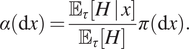 $$ \alpha \left(\mathrm{d}x\right)=\frac{{\unicode{x1D53C}}_{\tau}\left[H\hskip.2em |\hskip.2em x\right]}{{\unicode{x1D53C}}_{\tau}\left[H\right]}\pi \left(\mathrm{d}x\right). $$
 The interpretation of these results are as follows: if the chain  $ \left(X,\hskip.2em L\right)(t) $ is initialized at some time $ t=b<0 $ such that it is in stationary at time $ t=0 $, then $ X(0) $’s distribution is precisely given in Corollary 2. By Corollary 2, in stationarity, the likelihood of a particular $ x $ appearing is proportional to the likelihood $ \pi $ with which it arises under the original Markov chain, and the expected length of real time for which it holds when it does.
Corollary 3. Let  $ \left(X,\hskip.2em L\right)\sim \alpha $, then the conditional probability distribution of $ X $ given $ L<\epsilon $ is $ \pi $.
Corollary 3 simply recovers the original Markov chain from the Markov jump process. This result follows since  $ {\overline{F}}_{\tau}\left(l\hskip.2em |\hskip.2em x\right)=1 $ (of Proposition 1) for all $ x $ and $ l\hskip.4em \le \hskip.4em \epsilon $.
We refer to  $ \alpha $ as the anytime distribution. It is precisely the stationary distribution of the Markov jump process. The new name is introduced to distinguish it from the stationary distribution $ \pi $ of the original Markov chain, which we continue to refer to as the target distribution.
Finally, we state an ergodic theorem from Alsmeyer (Reference Alsmeyer1997); see also Alsmeyer (Reference Alsmeyer1994). Rather than study the process  $ \left(X,L\right)(t) $, we can equivalently study $ {\left({X}_n,{A}_n\right)}_{n=1}^{\infty } $, with the initial state being $ \left({X}_0,0\right) $. This is a Markov renewal process. Conditioned on $ {\left({X}_n\right)}_{n=0}^{\infty } $, the hold times $ {\left({H}_n\right)}_{n=0}^{\infty } $ are independent. This conditional independence can be exploited to derive ergodic properties of $ {\left({X}_n,{A}_n\right)}_{n=1}^{\infty } $, based on assumed regularity of the driving chain $ {\left({X}_n\right)}_{n=0}^{\infty } $.
Proposition 4 (Alsmeyer, Reference Alsmeyer1997, Corollary1). Assume that the Markov chain  $ {\left({X}_n\right)}_{n=1}^{\infty } $ is Harris recurrent. For a function $ g:\unicode{x1D54F}\to \mathrm{\mathbb{R}} $ with $ \int \left|g(x)\hskip0.2em \right|\hskip0.2em \alpha \left(\mathrm{d}x\right)<\infty $,
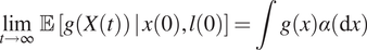 $$ \underset{t\to \infty }{\lim}\hskip0.4em \unicode{x1D53C}\hskip0.2em \left[g\left(X(t)\right)\hskip0.2em |\hskip0.2em x(0),l(0)\right]=\int g(x)\alpha \left(\mathrm{d}x\right) $$
for  $ \pi $-almost all $ x(0) $ and all $ l(0) $.
A further interpretation of this result confirms that, regardless of how we initialize the chain  $ \left(X,L\right)(t) $ at time $ t=0 $, at a future time $ t=T $ the distribution of $ X(T) $ is close to $ \alpha $ and approaches $ \alpha $ as $ T\to \infty $.
2.1. Establishing anytime behavior
The above results establish that, when interrupted at real time  $ t $, the state of a Monte Carlo computation is distributed according to the anytime distribution, $ \alpha $. We wish to establish situations in which it is instead distributed according to the target distribution, $ \pi $. This will allow us to draw samples of $ \pi $ simply by interrupting the running process at any time $ t $, and will form the basis of anytime Monte Carlo algorithms.
Recalling Corollary 2, a sufficient condition to establish  $ \alpha \left(\mathrm{d}x\right)=\pi \left(\mathrm{d}x\right) $ is that $ {\unicode{x1D53C}}_{\tau}\left[H|x\right]={\unicode{x1D53C}}_{\tau}\left[H\right] $, that is for the expected hold time to be independent of $ X $. For iid sampling, this is trivially the case: we have $ \kappa \left(\mathrm{d}x\hskip0.2em |\hskip0.2em {x}_{n-1}\right)=\pi \left(\mathrm{d}x\right) $, the hold time $ {H}_{n-1} $ for $ {X}_{n-1} $ is the time taken to draw $ {X}_n\sim \pi \left(\mathrm{d}x\right) $ and so is independent of $ {X}_{n-1} $, and $ {\unicode{x1D53C}}_{\tau}\left[H\hskip0.2em |\hskip0.2em x\right]={\unicode{x1D53C}}_{\tau}\left[H\right] $.
For non-iid sampling, first consider the following change to the Markov kernel:
 $$ {X}_n\hskip.2em \mid \hskip.2em {x}_{n-2}\sim \kappa \left(\mathrm{d}x\hskip0.2em |\hskip0.2em {x}_{n-2}\right). $$
That is, each new state  $ {X}_n $ depends not on the previous state, $ {x}_{n-1} $, but on one state back again, $ {x}_{n-2} $, so that odd- and even-numbered states are independent. The hold times of the even-numbered states are the compute times of the odd-numbered states and vice versa, so that hold times are independent of states, and the desired property $ {\unicode{x1D53C}}_{\tau}\left[H\hskip0.2em |\hskip0.2em x\right]={\unicode{x1D53C}}_{\tau}\left[H\right] $, and so $ \alpha \left(\mathrm{d}x\right)=\pi \left(\mathrm{d}x\right) $, is achieved. This sampling strategy is illustrated in Figure 2 where the odd chain is Chain 1 (Superscript 1) and the even chain is Chain 2. When querying the sampler at any time $ t $, the sampler returns the chain that is holding and not being worked, which is Chain 2 in the figure. It follows then that the returned sample is distributed according to $ \pi $ as desired. In an attempt to increase the efficiency of this procedure for SMC methods in Section 3, we extend the idea to $ K+1 $ chains as follows. The processor works/samples each of the $ K+1 $ chains in sequential order. At any time $ t $, when queried, all but one chain is being worked and the processor returns the states of the $ K $ chains that are not being worked on. Each state will then be an independent sample with distribution $ \pi $.
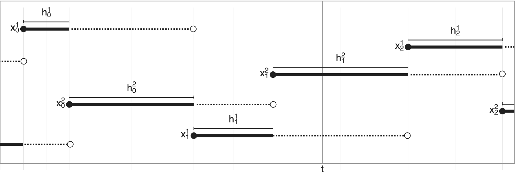
Figure 2. Illustration of the multiple chain concept with two Markov chains. At any time, one chain is being simulated (indicated with a dotted line) while one chain is waiting (indicated with a solid line). When querying the process at some time  $ t $, it is the state of the waiting chain that is reported, so that the hold times of each chain are the compute times of the other chain. For $ K+1\ge 2 $ chains, there is always one chain simulating while $ K $ chains wait, and when querying the process at some time $ t $, the states of all $ K $ waiting chains are reported.
Formally, suppose that we are simulating  $ K $ number of Markov chains, with $ K $ a positive integer, plus one extra chain. Denote these $ K+1 $ chains as $ {\left({X}_n^{1:K+1}\right)}_{n=0}^{\infty } $. For simplicity, assume that all have the same target distribution $ \pi $, kernel $ \kappa $, and hold time distribution $ \tau $. The joint target is
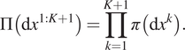 $$ \Pi \left(\mathrm{d}{x}^{1:K+1}\right)=\prod \limits_{k=1}^{K+1}\pi \left(\mathrm{d}{x}^k\right). $$
The  $ K+1 $ chains are simulated on the same processor, one at a time, in a serial schedule. To avoid introducing an index for the currently simulating chain, it is equivalent that chain $ K+1 $ is always the one simulating, but that states are rotated between chains after each jump. Specifically, the state of chain $ K+1 $ at step $ n-1 $ becomes the state of Chain 1 at step $ n $, and the state of each other chain $ k\in \left\{1,\dots, K\right\} $ becomes the state of chain $ k+1 $. The transition can then be written as
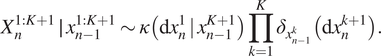 $$ {X}_n^{1:K+1}\hskip.2em \mid \hskip.2em {x}_{n-1}^{1:K+1}\sim \kappa \left(\mathrm{d}{x}_n^1\hskip0.2em |\hskip0.2em {x}_{n-1}^{K+1}\right)\prod \limits_{k=1}^K{\delta}_{x_{n-1}^k}\left(\mathrm{d}{x}_n^{k+1}\right). $$
As before, this joint Markov chain has an associated joint Markov jump process  $ \left({X}^{1:K+1},\hskip.2em L\right)(t) $, where $ L(t) $ is the lag time elapsed since the last jump. This joint Markov jump process is readily manipulated to yield the following properties, analogous to the single chain case. Proofs are given in Appendix A in Supplementary Material.
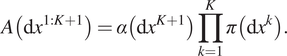
Proposition 5. The stationary distribution of the Markov jump process  $ \left({X}^{1:K+1},L\right)(t) $ is
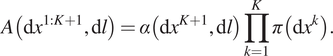 $$ A\left(\mathrm{d}{x}^{1:K+1},\mathrm{d}l\right)=\alpha \left(\mathrm{d}{x}^{K+1},\mathrm{d}l\right)\prod \limits_{k=1}^K\pi \left(\mathrm{d}{x}^k\right). $$
 This result for the joint process extrapolates Proposition 1. To see this, note that the key ingredients of Proposition 1,  $ {\overline{F}}_{\tau}\left(l\hskip0.2em |\hskip0.2em x\right) $ and $ \pi \left(\mathrm{d}x\right) $, are now replaced with $ {\overline{F}}_{\tau}\left(l\hskip0.2em |\hskip0.2em {x}^{K+1}\right) $ and $ \Pi \left(\mathrm{d}{x}^{1:K+1}\right) $. The hold-time survival function for the product chain is $ {\overline{F}}_{\tau}\left(l\hskip0.2em |\hskip0.2em {x}^{K+1}\right) $, since it related to the time taken to execute the kernel $ \kappa \left(\mathrm{d}{x}_n^1\hskip0.2em |\hskip0.2em {x}_{n-1}^{K+1}\right) $, which depends on the state of chain $ K+1 $ only.
Corollary 6. With respect to  $ \Pi \left(\mathrm{d}{x}^{1:K+1}\right) $, $ A\left(\mathrm{d}{x}^{1:K+1}\right) $ is length-biased by expected hold time on the extra state $ {X}^{K+1} $ only:
 $$ A\left(\mathrm{d}{x}^{1:K+1}\right)=\alpha \left(\mathrm{d}{x}^{K+1}\right)\prod \limits_{k=1}^K\pi \left(\mathrm{d}{x}^k\right). $$
Corollary 7. Let  $ \left({X}^{1:K+1},L\right)\sim A $, then the conditional probability distribution of $ {X}^{1:K+1} $ given $ L<\epsilon $ is $ \Pi \left(\mathrm{d}{x}^{1:K+1}\right) $.
We state without proof that the product chain construction also satisfies the ergodic theorem under the same assumptions as Proposition 4. Numerical validation is given in Section 4.1.
The practical implication of these properties is that any MCMC algorithm running  $ K\hskip.2em \ge \hskip.2em 1 $ chains can be converted into an anytime MCMC algorithm by interleaving one extra chain. When the computation is interrupted at some time $ t $, the state of the extra chain is distributed according to $ \alpha $, while the states of the remaining $ K $ chains are independently distributed according to $ \pi $. The state of the extra chain is simply discarded to eliminate the length bias.
3. Methods
It is straightforward to apply the above framework to design anytime MCMC algorithms. One simply runs  $ K+1 $ chains of the desired MCMC algorithm on a single processor, using a serial schedule, and eliminating the state of the extra chain whenever the computation is interrupted at some real time $ t $. The anytime framework is particularly useful within a broader SMC method (Del Moral et al., Reference Del Moral, Doucet and Jasra2006), where there already exist multiple chains (particles) with which to establish anytime behavior. We propose appropriate SMC methods in this section.
3.1. Sequential Monte Carlo
We are interested in the context of sequential Bayesian inference targeting a posterior distribution  $ \pi \left(\mathrm{d}x\right)=p\left(\mathrm{d}x\hskip0.2em |\hskip0.2em {y}_{1:V}\right) $ for a given dataset $ {y}_{1:V} $. For the purposes of SMC, we assume that the target distribution $ \pi \Big(\mathrm{d}x $) admits a density $ \pi (x) $ in order to compute importance weights.
Define a sequence of target distributions  $ {\pi}_0\left(\mathrm{d}x\right)=p\left(\mathrm{d}x\right) $ and $ {\pi}_v\left(\mathrm{d}x\right)\hskip.2em \propto \hskip.2em p\left(\mathrm{d}x\hskip.2em |\hskip.2em {y}_{1:v}\right) $ for $ v=1,\dots, V $. The first target equals the prior distribution, while the final target equals the posterior distribution, $ {\pi}_V\left(\mathrm{d}x\right)=p\left(\mathrm{d}x\hskip.2em |\hskip.2em {y}_{1:V}\right)=\pi \left(\mathrm{d}x\right) $. Each target $ {\pi}_v $ has an associated Markov kernel $ {\kappa}_v $, invariant to that target, which could be defined using an MCMC algorithm.
An SMC algorithm propagates a set of weighted samples (particles) through the sequence of target distributions. At step  $ v $, the target $ {\pi}_v\left(\mathrm{d}x\right) $ is represented by an empirical approximation $ {\hat{\pi}}_v\left(\mathrm{d}x\right) $, constructed with $ K $ number of samples $ {x}_v^{1:K} $ and their associated weights $ {w}_v^{1:K} $:
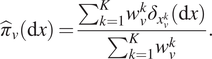 $$ {\hat{\pi}}_v\left(\mathrm{d}x\right)=\frac{\sum_{k=1}^K{w}_v^k{\delta}_{x_v^k}\left(\mathrm{d}x\right)}{\sum_{k=1}^K{w}_v^k}. $$
A basic SMC algorithm proceeds as in Algorithm 1.
Algorithm 1. A basic SMC algorithm. Where  $ k $ appears, the operation is performed for all $ k\in \left\{1,\dots, K\right\} $.
1. Initialize $ {x}_0^k\sim {\pi}_0\left(\mathrm{d}{x}_0\right) $.

2. For  $ v=1,\dots, V $
(a) Set  $ {x}_v^k={x}_{v-1}^k $ and weight $ {w}_v^k={\pi}_v\left({x}_v^k\right)/{\pi}_{v-1}\left({x}_v^k\right)\hskip.2em \propto \hskip.2em p\left({y}_v\hskip0.2em |\hskip0.2em {x}_v^k{y}_{1:v-1}\right) $, to form the empirical approximation $ {\hat{\pi}}_v\left(\mathrm{d}{x}_v\right)\hskip.2em \approx \hskip.2em {\pi}_v\left(\mathrm{d}{x}_v\right) $.
(b) Resample  $ {x}_v^k\sim {\hat{\pi}}_v\left(\mathrm{d}{x}_v\right) $.
(c) Move  $ {x}_v^k\sim {\kappa}_v\left(\mathrm{d}{x}_v|{x}_v^k\right) $ for $ {n}_v $ steps.
An extension of the algorithm concerns the case where the sequence of target distributions requires marginalizing over some additional latent variables. In these cases, a pseudomarginal approach (Andrieu and Roberts, Reference Andrieu and Roberts2009) can be adopted, replacing the exact weight computations with unbiased estimates (Fearnhead et al., Reference Fearnhead, Papaspiliopoulos and Roberts2008, Reference Fearnhead, Papaspiliopoulos, Roberts and Stuart2010). For example, for a state-space model at step  $ v $, there are $ v $ hidden states $ {z}_{1:v}\in {\mathrm{\mathbb{Z}}}^v $ to marginalize over:
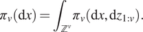 $$ {\pi}_v\left(\mathrm{d}x\right)={\int}_{{\mathrm{\mathbb{Z}}}^v}{\pi}_v\left(\mathrm{d}x,\mathrm{d}{z}_{1:v}\right). $$
Unbiased estimates of this integral can be obtained by a nested SMC procedure targeting  $ {\pi}_v\left(\mathrm{d}{z}_{1:v}|x\right) $, leading to the algorithm known as SMC $ {}^2 $ (Chopin et al., Reference Chopin, Jacob and Papaspiliopoulos2013), where the kernels $ {\kappa}_v $ are particle MCMC moves (Andrieu et al., Reference Andrieu, Doucet and Holenstein2010). This is used for the example of Section 4.2.
3.2. SMC with anytime moves
In the conventional SMC algorithm, it is necessary to choose  $ {n}_v $, the number of kernel moves to make per particle in Step 2(c). For anytime moves, this is replaced with a real-time budget $ {t}_v $. Move steps are typically the most expensive steps—certainly so for SMC $ {}^2 $—with the potential for significant variability in the time taken to move each particle. An anytime treatment provides control over the budget of the move step which, if it is indeed the most expensive step, provides substantial control over the total budget also.
The anytime framework is used as follows. Associated with each target distribution  $ {\pi}_v $, and its kernel $ {\kappa}_v $, is a hold time distribution $ {\tau}_v $, and implied anytime distribution $ {\alpha}_v $. At step $ v $, after resampling, an extra particle and lag $ \left({x}_v^{K+1},\hskip.2em {l}_v\right) $ are drawn (approximately) from the anytime distribution $ {\alpha}_v $. The real-time Markov jump process $ \left({X}_v^{1:K+1},\hskip.2em {L}_v\right)(t) $ is then initialized with these particles and lag, and simulated forward until time $ {t}_v $ is reached. The extra chain and lag are then eliminated, and the states of the remaining chains are restored as the $ K $ particles $ {x}_v^{1:K} $.
The complete algorithm is given in Algorithm 2.
Algorithm 2. SMC with anytime moves. Where  $ k $ appears, the operation is performed for all $ k\in \left\{1,\dots, K\right\} $.
1. Initialize
$ {x}_0^k\sim {\pi}_0\left(\mathrm{d}{x}_0\right) $.

2. For  $ v=1,\dots, V $
(a) Set  $ {x}_v^k={x}_{v-1}^k $ and weight $ {w}_v^k={\pi}_v\left({x}_v^k\right)/{\pi}_{v-1}\left({x}_v^k\right)\hskip.2em \propto \hskip.4em p\left({y}_v\hskip0.2em |\hskip0.2em {x}_v^k{y}_{1:v-1}\right) $, to form the empirical approximation $ {\hat{\pi}}_v\left(\mathrm{d}{x}_v\right)\hskip.2em \approx \hskip.2em {\pi}_v\left(\mathrm{d}{x}_v\right) $.
(b) Resample  $ {x}_v^k\sim {\hat{\pi}}_v\left(\mathrm{d}{x}_v\right) $.
(c) Draw (approximately) an extra particle and lag  $ \left({x}_v^{K+1},\hskip.2em {l}_v\right)\sim {\alpha}_v\left(\mathrm{d}{x}_v,\hskip.2em \mathrm{d}{l}_v\right) $. Construct the real-time Markov jump process $ \left({X}_v^{1:K+1},\hskip.2em {L}_v\right)(0)=\left({x}_v^{1:K+1},\hskip.2em {l}_v\right) $ and simulate it forward for some real time $ {t}_v $. Set $ {x}_v^{1:K}={X}_v^{1:K}\left({t}_v\right) $, discarding the extra particle and lag.
By the end of the move Step 2(c), as  $ {t}_v\to \infty $, the particles $ {x}_v^{1:K+1} $ become distributed according to $ {A}_v $, regardless of their distribution after the resampling Step 2(b). This is assured by Proposition 4. After eliminating the extra particle, the remaining $ {x}_v^{1:K} $ are distributed according to $ {\Pi}_v $.
In practice, of course, it is necessary to choose some finite  $ {t}_v $ for which the $ {x}_v^{1:K} $ are distributed only approximately according to $ {\Pi}_v $. For any given $ {t}_v $, their divergence in distribution from $ {\Pi}_v $ is minimized by an initialization as close as possible to $ {A}_v $. We have, already, the first $ K $ chains initialized from an empirical approximation of the target, $ {\hat{\pi}}_v $, which is unlikely to be improved upon. We need only consider the extra particle and lag.
An easily-implemented choice is to draw  $ \left({x}_v^{K+1},\hskip.2em {l}_v\right)\sim {\hat{\pi}}_v\left(\mathrm{d}{x}_v\right){\delta}_0\left(\mathrm{d}{l}_v\right) $. In practice, this merely involves resampling $ K+1 $ rather than $ K $ particles in Step 2(b), setting $ {l}_v=0 $ and proceeding with the first move.
An alternative is  $ \left({x}_v^{K+1},\hskip.2em {l}_v\right)\sim {\delta}_{x_{v-1}^{K+1}}\left(\mathrm{d}{x}_v\right){\delta}_{l_{v-1}}\left(\mathrm{d}{l}_v\right) $. This resumes the computation of the extra particle that was discarded at step $ v-1 $. As $ {t}_{v-1}\to \infty $, it amounts to approximating $ {\alpha}_v $ by $ {\alpha}_{v-1} $, which is sensible if the sequence of anytime distributions changes only slowly.
3.3. Distributed SMC with anytime moves
While the potential to parallelize SMC is widely recognized (see e.g., Lee et al., Reference Lee, Yau, Giles, Doucet and Holmes2010; Murray, Reference Murray2015), the resampling Step 2(b) in Algorithm 1 is acknowledged as a potential bottleneck when in a distributed computing environment of  $ P $ number of processors. This is due to collective communication: all processors must synchronize after completing the preceding steps in order for resampling to proceed. Resampling cannot proceed until the slowest among them completes. As this is a maximum among $ P $ processors, the expected wait time increases with $ P $. Recent work has considered either global pairwise interaction (Murray, Reference Murray2011; Murray et al., Reference Murray, Lee and Jacob2016) or limited interaction (Vergé et al., Reference Vergé, Dubarry, Del Moral and Moulines2015; Lee and Whiteley, Reference Lee and Whiteley2016; Whiteley et al., Reference Whiteley, Lee and Heine2016) to address this issue. Instead, we propose to preserve collective communication, but to use an anytime move step to ensure the simultaneous readiness of all processors for resampling.
SMC with anytime moves is readily distributed across multiple processors. The  $ K $ particles are partitioned so that processor $ p\in \left\{1,\dots, P\right\} $ has some number of particles, denoted $ {K}^p $, and so that $ {\sum}_{p=1}^P{K}^p=K $. Each processor can proceed with initialization, move and weight steps independently of the other processors. After the resampling step, each processor has $ {K}^p $ number of particles. During the move step, each processor draws its own extra particle and lag from the anytime distribution, giving it $ {K}^p+1 $ particles, and discards them at the end of the step leaving it with $ {K}^p $ again. Collective communication is required for the resampling step, and an appropriate distributed resampling scheme should be used (see e.g., Bolić et al., Reference Bolić, Djurić and Hong2005; Vergé et al., Reference Vergé, Dubarry, Del Moral and Moulines2015; Lee and Whiteley, Reference Lee and Whiteley2016).
In the simplest case, all workers have homogeneous hardware and the obvious partition of particles is  $ {K}^p=K/P $. For heterogeneous hardware another partition may be set a priori (see e.g., Rosenthal, Reference Rosenthal2000). Note also that with heterogenous hardware, each processor may have a different compute capability and therefore different distribution $ {\tau}_v $. For processor $ p $, we denote this $ {\tau}_v^p $ and the associated anytime distribution $ {\alpha}_v^p $. This difference between processors is easily accommodated, as the anytime treatment is local to each processor.
A distributed SMC algorithm with anytime moves proceeds as in Algorithm 3.
Algorithm 3. SMC with anytime moves. Where  $ k $ appears, the operation is performed for all $ k\in \left\{1,\dots, {K}^p\right\} $.
1. On each processor
$ p $, initialize $ {x}_0^k\sim {\pi}_0\left(\mathrm{d}x\right) $.


2. For  $ v=1,\dots, V $
(a) On each processor  $ p $, set $ {x}_v^k={x}_{v-1}^k $ and weight $ {w}_v^k={\pi}_v\left({x}_v^k\right)/{\pi}_{v-1}\left({x}_v^k\right)\hskip.2em \propto \hskip.4em p\left({y}_v\hskip0.2em |\hskip0.2em {x}_v^k,{y}_{1:v-1}\right) $. Collectively, all $ K $ particles form the empirical approximation $ {\hat{\pi}}_v\left(\mathrm{d}{x}_v\right)\hskip.2em \approx \hskip.2em {\pi}_v\left(\mathrm{d}{x}_v\right) $.
(b) Collectively resample  $ {x}_v^k\sim {\hat{\pi}}_v\left(\mathrm{d}{x}_v\right) $ and redistribute the particles among processors so that processor $ p $ has exactly $ {K}^p $ particles again.
(c) On each processor  $ p $, draw (approximately) an extra particle and lag $ \left({x}_v^{K^p+1},{l}_v\right)\sim {\alpha}_v^p\left(\mathrm{d}x,\mathrm{d}l\right) $. Construct the real-time process $ \left({X}_v^{1:{K}^p+1},{L}_v\right)(0)=\left({x}_v^{1:{K}^p+1},{l}_v\right) $ and simulate it forward for some real time $ {t}_v $. Set $ {x}_v^{1:{K}^p}={X}_v^{1:{K}^p}\left({t}_v\right) $, discarding the extra particle and lag.
The preceding discussion around the approximate anytime distribution still holds for each processor in isolation: for any given budget  $ {t}_v $, to minimize the divergence between the distribution of particles and the target distribution, $ {\hat{A}}_v^p $ should be chosen as close as possible to $ {A}_v^p $.
3.4. Setting the compute budget
We set an overall compute budget for move steps, which we denote  $ t $, and apportion this into a quota for each move step $ v $, which we denote $ {t}_v $ as above. This requires some a priori knowledge of the compute profile for the problem at hand.
Given  $ {\hat{\pi}}_{v-1} $, if the compute time necessary to obtain $ {\hat{\pi}}_v $ is constant with respect to $ v $, then a suitable quota for the $ v $th move step is the obvious $ {t}_v=t/V $. If, instead, the compute time grows linearly in $ v $, as is the case for SMC $ {}^2 $, then we expect the time taken to complete the $ v $th step to be proportional to $ v+c $ (where the constant $ c $ is used to capture overheads). A sensible quota for the $ v $th move step is then
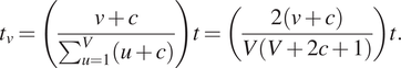 $$ {t}_v=\left(\frac{v+c}{\sum_{u=1}^V\left(u+c\right)}\right)t=\left(\frac{2\left(v+c\right)}{V\left(V+2c+1\right)}\right)t. $$
For the constant, a default choice might be  $ c=0 $; higher values shift more time to earlier time steps.
This approximation does neglect some complexities. The use of memory-efficient path storage (Jacob et al., Reference Jacob, Murray and Rubenthaler2015), for example, introduces a time-dependent contribution of  $ \mathcal{O}(K) $ at $ v=1 $, increasing to $ \mathcal{O}\left(K\log K\right) $ with $ v $ as the ancestry tree grows. Nonetheless, for the example of Section 4.2 we observe, anecdotally, that this partitioning of the time budget produces surprisingly consistent results with respect to the random number of moves completed at each move step $ v $.
3.5. Resampling considerations
To reduce the variance in resampling outcomes (Douc and Cappé, Reference Douc and Cappé2005), implementations of SMC often use schemes such as systematic, stratified (Kitagawa, Reference Kitagawa1996) or residual (Liu and Chen, Reference Liu and Chen1998) resampling, rather than the multinomial scheme (Gordon et al., Reference Gordon, Salmond and Smith1993) with which the above algorithms have been introduced. The implementation of these alternative schemes does not necessarily leave the random variables  $ {X}_v^1,\dots, {X}_v^K $ exchangeable; for example, the offspring of a particle are typically neighbors in the output of systematic or stratified resampling (see e.g., Murray et al., Reference Murray, Lee and Jacob2016).
Likewise, distributed resampling schemes do not necessarily redistribute particles identically between processors. For example, the implementation in LibBi (Murray, Reference Murray2015) attempts to minimize the transport of particles between processors, such that the offspring of a parent particle are more likely to remain on the same processor as that particle. This means that the distribution of the  $ {K}^p $ particles on each processor may have greater divergence from $ {\pi}_v $ than the distribution of the $ K $ particles overall.
In both cases, the effect is that particles are initialized further from the ideal  $ {A}_v $. Proposition 4 nonetheless ensures consistency as $ {t}_v\to \infty $. A random permutation of particles may result in a better initialization, but this can be costly, especially in a distributed implementation where particles must be transported between processors. For a fixed total budget, the time spent permuting may be better spent by increasing $ {t}_v $. The optimal choice is difficult to identify in general; we return to this point in the discussion.
4. Experiments
This section presents two case studies to empirically investigate the anytime framework and the proposed SMC methods. The first uses a simple model where real-time behavior is simulated in order to validate the results of Section 2. The second considers a Lorenz ’96 state-space model with nontrivial likelihood and compute profile, testing the SMC methods of Section 3 in two real-world computing environments.
4.1. Simulation study
Consider the model
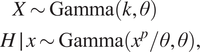 $$ {\displaystyle \begin{array}{l}\hskip1em X\sim \mathrm{Gamma}\left(k,\theta \right)\\ {}H\hskip.2em \mid \hskip.2em x\sim \mathrm{Gamma}\left({x}^p/\theta, \theta \right),\end{array}} $$
with shape parameter  $ k $, scale parameter $ \theta $, and polynomial degree $ p $. The two Gamma distributions correspond to $ \pi $ and $ \tau $, respectively. The anytime distribution is:
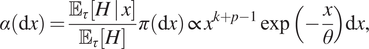 $$ \alpha \left(\mathrm{d}x\right)=\frac{{\unicode{x1D53C}}_{\tau}\left[H\hskip0.2em |\hskip0.2em x\right]}{{\unicode{x1D53C}}_{\tau}\left[H\right]}\pi \left(\mathrm{d}x\right)\hskip.2em \propto \hskip.2em {x}^{k+p-1}\exp \left(-\frac{x}{\theta}\right)\mathrm{d}x, $$
which is  $ \mathrm{Gamma}\left(k+p,\theta \right) $.
Of course, in real situations,  $ \tau $ is not known explicitly, and is merely implied by the algorithm used to simulate $ X $. For this first study, however, we assume the explicit form above and simulate virtual hold times. This permits exploration of the real-time effects of polynomial computational complexity in a controlled environment, including constant ( $ p=0 $), linear ( $ p=1 $), quadratic ( $ p=2 $) and cubic ( $ p=3 $) complexity.
To construct a Markov chain  $ {\left({X}_n\right)}_{n=0}^{\infty } $ with target distribution $ \mathrm{Gamma}\left(k,\theta \right) $, first consider a Markov chain $ {\left({Z}_n\right)}_{n=0}^{\infty } $ with target distribution $ \mathcal{N}\left(0,1\right) $ and kernel
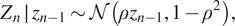 $$ {Z}_n\hskip.2em \mid \hskip.2em {z}_{n-1}\sim \mathcal{N}\left(\rho {z}_{n-1},1-{\rho}^2\right), $$
where  $ \rho $ is an autocorrelation parameter. Now define $ {\left({X}_n\right)}_{n=0}^{\infty } $ as
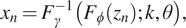 $$ {x}_n={F}_{\gamma}^{-1}\left({F}_{\phi}\left({z}_n\right);k,\theta \right), $$
where  $ {F}_{\gamma}^{-1} $ is the inverse cdf of the Gamma distribution with parameters $ k $ and $ \theta $, and $ {F}_{\phi } $ is the cdf of the standard normal distribution. By construction, $ \rho $ parameterizes a Gaussian copula inducing correlation between adjacent elements of $ {\left({X}_n\right)}_{n=0}^{\infty } $.
For the experiments in this section, we set  $ k=2 $, $ \theta =1/2 $, $ \rho =1/2 $, and use $ p\hskip.2em \in \hskip.2em \left\{\mathrm{0,1,2,3}\right\} $. In all cases Markov chains are initialized from $ \pi $ and simulated for 200 units of virtual time.
We employ the one-Wasserstein distance to compare distributions. For two univariate distributions  $ \mu $ and $ \nu $ with associated cdfs $ {F}_{\mu }(x) $ and $ {F}_{\nu }(x) $, the one-Wasserstein distance $ {d}_1\left({F}_{\mu },{F}_{\nu}\right) $ can be evaluated as (Shorack and Wellner, Reference Shorack and Wellner1986, p. 64)
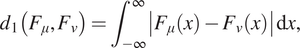 $$ {d}_1\left({F}_{\mu },{F}_{\nu}\right)={\int}_{-\infty}^{\infty}\left|{F}_{\mu }(x)-{F}_{\nu }(x)\right|\hskip0.1em \mathrm{d}x, $$
which, for the purposes of this example, is sufficiently approximated by numerical integration. The first distribution will always be the empirical distribution of a set of  $ n $ samples, its cdf denoted $ {F}_n(x) $. If those samples are distributed according to the second distribution, the distance will go to zero as $ n $ increases. See Figure 3.
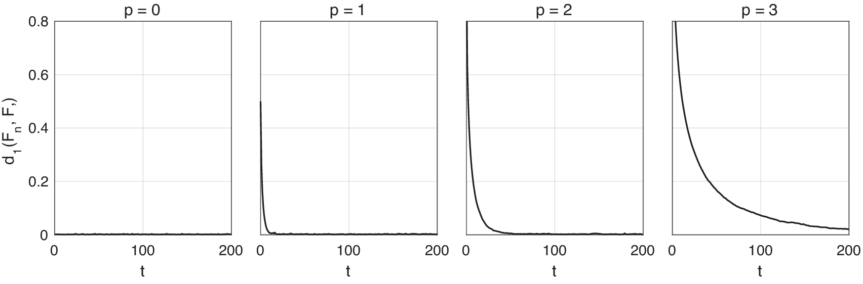
Figure 3. Convergence of Markov chains to the anytime distribution for the simulation study, with constant ( $ p=0 $), linear ( $ p=1 $), quadratic ( $ p=2 $), and cubic ( $ p=3 $) expected hold time. Each plot shows the evolution of the one-Wasserstein distance between the anytime distribution and the empirical distribution of $ {2}^{18} $ independent Markov chains initialized from the target distribution.
4.1.1. Validation of the anytime distribution
We first validate, empirically, that the anytime distribution is indeed  $ \mathrm{Gamma}\left(k+p,\theta \right) $ as expected. We simulate $ n={2}^{18} $ Markov chains. At each integer time we take the state of all $ n $ chains to construct an empirical distribution. We then compute the one-Wasserstein distance between this and the anytime distribution, using the empirical cdf $ {F}_n(x) $ and anytime cdf $ {F}_{\alpha }(x) $.
Figure 2 plots the results over time. In all cases the distance goes to zero in  $ t $, slower for larger $ p $. This affirms the theoretical results obtained in Section 2.
4.1.2. Validation of the multiple chain strategy
We next check the efficacy of the multiple chain strategy in eliminating length bias. For  $ K+1\in \left\{\mathrm{2,4,8,16,32}\right\} $, we initialize $ K+1 $ chains and simulate them forward in a serial schedule. For $ n={2}^{18} $, this is repeated $ n/\left(K+1\right) $ times. We then consider ignoring the length bias versus correcting for it. In the first case, we take the states of all $ K+1 $ chains at each time, giving $ n $ samples from which to construct an empirical cdf $ {F}_n(x) $. In the second case, we eliminate the extra chain but keep the remaining $ K $, giving $ nK/\left(K+1\right) $ samples from which to construct an empirical cdf $ {F}_{nK/\left(K+1\right)}(x) $. In both cases, we compute the one-Wasserstein distance between the empirical and target distributions, using the appropriate empirical cdf, and the target cdf $ {F}_{\pi }(x) $.
Figure 4 plots the results over time for both the uncorrected (top) and corrected (bottom) cases. For the uncorrected case, the one-Wasserstein distance between the empirical distribution and target distribution does not converge to zero. Neither does it become arbitrarily bad: the distance is due to one of the  $ K+1 $ chains being distributed according to $ \alpha $ and not $ \pi $, the influence of which decreases as $ K $ increases.
Figure 4. Correction of length bias for the simulation study, using  $ K+1\in \left\{\mathrm{2,4,8,16,32}\right\} $ chains (light to dark), with constant ( $ p=0 $), linear ( $ p=1 $), quadratic ( $ p=2 $), and cubic ( $ p=3 $) expected hold time. Each plot shows the evolution of the one-Wasserstein distance between the empirical and target distributions. On the top row, the states of all chains contribute to the empirical distribution, which does not converge to the target. On the bottom row, the state of the extra chain is eliminated, contributing only the remaining states to the empirical distribution, which does converge to the target.
For the corrected case, where the extra chain is eliminated, the distance converges to zero in time. This confirms the efficacy of the multiple chain strategy in yielding an anytime distribution equal to the target distribution.
4.2. Distributed computing study
Consider a stochastic extension of the deterministic Lorenz ’96 (Lorenz, Reference Lorenz2006) model described by the stochastic differential equation (SDE)
 $$ \mathrm{d}{X}_d=\left({X}_{d-1}\left({X}_{d+1}-{X}_{d-2}\right)-{X}_d+F\right)\hskip0.1em \mathrm{d}t+\sigma \hskip0.1em \mathrm{d}{W}_d, $$
with parameter  $ F $, constant $ \sigma $, state vector $ \mathbf{X}(t)\in {\mathrm{\mathbb{R}}}^D $, and Wiener process vector $ \mathbf{W}(t)\in {\mathrm{\mathbb{R}}}^D $, with elements of those vectors indexed cyclically by subscripts (i.e., $ {X}_{d-D}\equiv {X}_d\equiv {X}_{d+D} $). The SDE may be equivalently interpreted in the Ito or Stratonovich sense, as the noise term is additive (Kloeden and Platen, Reference Kloeden and Platen1992, p. 157). The observation model is given by
 $$ {Y}_d(t)\sim \mathbf{\mathcal{N}}\left({x}_d(t),{\boldsymbol{\varsigma}}^2\right). $$
We fix  $ D=8 $, $ {\sigma}^2={10}^{-4} $, $ {\varsigma}^2={10}^{-6} $ and set a prior on the parameter $ F $ and initial conditions $ \mathbf{X}(0) $ of:
 $$ {\displaystyle \begin{array}{c}F\sim \mathbf{\mathcal{U}}\left(\left[0,7\right]\right)\\ {}{X}_d(0)\sim \mathbf{\mathcal{N}}\left(0,{\sigma}^2\right).\end{array}} $$
The SDE can be approximately decomposed into a deterministic drift component given by the ordinary differential equation (ODE)
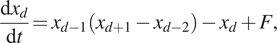 $$ \frac{\mathrm{d}{x}_d}{\mathrm{d}t}={x}_{d-1}\left({x}_{d+1}-{x}_{d-2}\right)-{x}_d+F, $$
and a diffusion component given by the Wiener process. On a fixed time step  $ \Delta t=5\times {10}^{-2} $, the drift component is first simulated using an appropriate numerical scheme for ODEs. Then, a Wiener process increment $ \Delta {W}_d\sim \mathbf{\mathcal{N}}\left(0,\Delta t\right) $ is simulated and added to the result. This numerical scheme yields a result similar to that of Euler–Maruyama for the original SDE but, for drift, substitutes the usual first-order Euler method with a higher-order Runge–Kutta method. This is advantageous in low-noise regimes where $ \sigma $ is close to zero, as here. In such cases, the dynamics are drift-dominated and can benefit from the higher-order scheme (see e.g., Milstein and Tretyakov, Reference Milstein and Tretyakov2004, chapter 3).
The RK4(3)5[2R+]C algorithm of Kennedy et al. (Reference Kennedy, Carpenter and Lewis2000) is used to simulate the drift. This provides a fourth order solution to the ODE with an embedded third-order solution for error estimates. Adaptive step-size adjustment is then used as in Hairer et al. (Reference Hairer, Nørsett and Wanner1993). The complete method is implemented (Murray, Reference Murray2012) on a graphics processing unit (GPU) as in the LibBi software (www.libbi.org; Murray, Reference Murray2015).
The Lorenz ’96 model exhibits intricate qualitative behaviors that depend on the parameter  $ F $. These range from decay, to periodicity, to chaos and back again (Figure 5, top row). With an adaptive step-size adjustment, the number of steps required to simulate trajectories within given error bounds generally increases with $ F $, so that compute time does also.
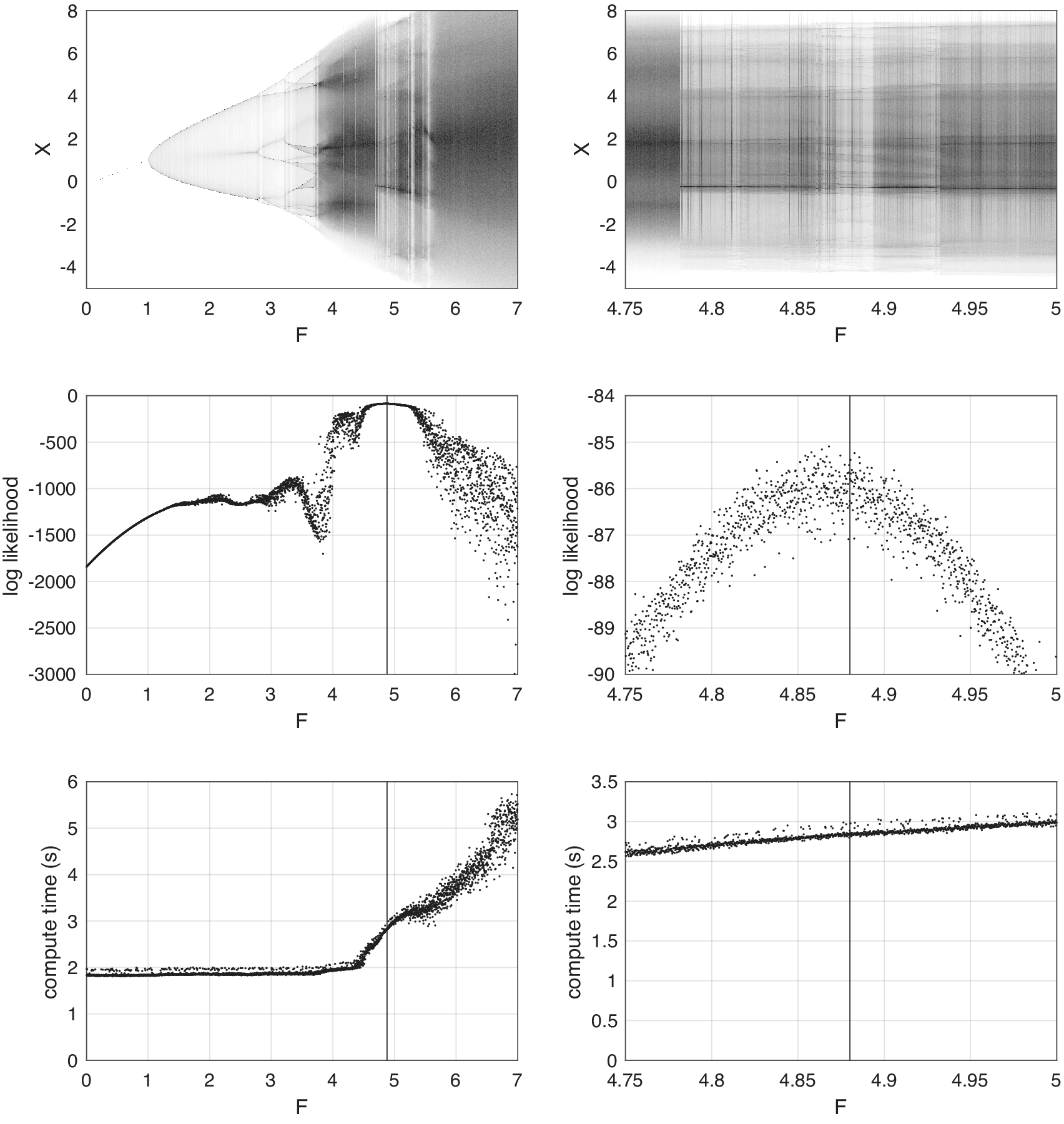
Figure 5. Elucidating the Lorenz ’96 model. The left column shows the range  $ F\hskip.2em \in \hskip.2em \left[0,7\right] $ as in the uniform prior distribution, while the right column shows a narrower range of $ F $ in the vicinity of the posterior distribution. The solid vertical lines indicate the value $ F=4.8801 $, with which data are simulated. The first row is a bifurcation diagram depicting the stationary distribution of any element of $ \mathbf{X}(t) $ for various values of $ F $. Each column is a density plot for a particular value of $ F $; darker for higher density values, scaled so that the mode is black. Note the intricate behaviors of decay, periodicity, and chaos induced by $ F $. The second row depicts estimates of the marginal log-likelihood of the simulated dataset for the same values of $ F $, using SMC with $ {2}^{20} $ particles. Multiple modes and heteroskedasticity are apparent. The third row depicts the compute time taken to obtain these estimates, showing increasing compute time in $ F $ after an initial plateau.
We produce a dataset by setting  $ F=4.8801 $, simulating a single trajectory for 10 time units and taking partial observations $ {\mathbf{Y}}_{1:4}(t) $ every 0.4 time units. This gives 100 observations in total. We then use SMC $ {}^2 $ to attempt to recover the correct posterior distribution over $ F $ given this dataset. This is nontrivial: this particular value of $ F $ is in a region where the qualitative behavior of the Lorenz ’96 model appears to switch frequently, in $ F $, between periodic and chaotic regimes (Figure 5, top right), suggesting that the marginal likelihood may not be smooth in the region of the posterior, and inference may be difficult.
The marginal likelihood  $ p\left(y\hskip0.2em |\hskip0.2em F\right) $ cannot be computed exactly, but it can be unbiasedly estimated with SMC. For each value of $ F $ on a regular grid, we run SMC with $ {2}^{20} $ particles to estimate the marginal likelihood. These estimates are shown in the middle left of Figure 5. The likelihood is clearly multi-modal, and the estimator heteroskedastic. Nevertheless, the variance in the estimator is tolerable in the region of the posterior distribution (middle right of Figure 5), suggesting that $ F $ can be recovered. The real time taken to compute these estimates is shown in the lower plots of Figure 5. The computations were performed in a random order through the grid points on $ F $ so as to decorrelate $ F $ with any transient exogenous effects on compute time. There appears, in fact, to have been some such effect: note the dotted line of points above the bulk on each plot, suggesting that a subset of runs have been slowed. This is most likely due to a contesting process on the shared server on which these computations were run. As expected, compute time tends to increase in $ F $ (after an initial plateau where other factors dominate). Furthermore, variance appears to increase with $ F $ in the higher regions.
We now run SMC $ {}^2 $ using the LibBi software on two platforms:
1. A shared-memory machine with 8 GPUs, each with 1,536 cores, for approximately 12,000-way parallelism, using
$ {2}^{10} $ particles for $ F $, each with $ {2}^{20} $ particles for $ \mathbf{X}(t) $, for approximately 1 billion particles overall. This is a shared machine where contestation from other jobs is expected.2. A distributed-memory cluster on the Amazon EC2 service, with 128 GPUs, each with 1,536 cores, for approximately 200,000-way parallelism, using
$ {2}^{12} $ particles for $ F $, each with $ {2}^{20} $ particles for X(t), for approximately 4 billion particles overall. This is a dedicated cluster where contestation from other jobs is not expected.


In order to obtain a more repeatable comparison between conventional SMC $ {}^2 $ and SMC $ {}^2 $ with anytime moves, we choose to use the same number of samples of $ \mathbf{X}(t) $ for all time steps, rather than adapting this in time as recommended in Chopin et al. (Reference Chopin, Jacob and Papaspiliopoulos2011). For the same reason, we resample at all steps rather than use an adaptive trigger. With anytime moves, the extra particle and lag are drawn as $ \left({x}_v^{K+1},{l}_v\right)\sim {\hat{\pi}}_v\left(\mathrm{d}{x}_v\right){\delta}_0\left(\mathrm{d}{l}_v\right) $.
We first run conventional SMC $ {}^2 $, making $ {n}_v=10 $ moves per particle at each step $ v $. We then run SMC $ {}^2 $ with anytime moves, prescribing a total budget for move steps of 60 min for the 8 GPU configuration, and 5 min for the 128 GPU configuration, apportioned as in equation (3).
The results of the 128 GPU runs are given in Figure 6. Recalling that  $ F=4.8801 $ for the simulated dataset, these suggest that the posterior has indeed been recovered successfully, and there is no indication that the posterior obtained with anytime move steps is much different from that obtained using the conventional method.
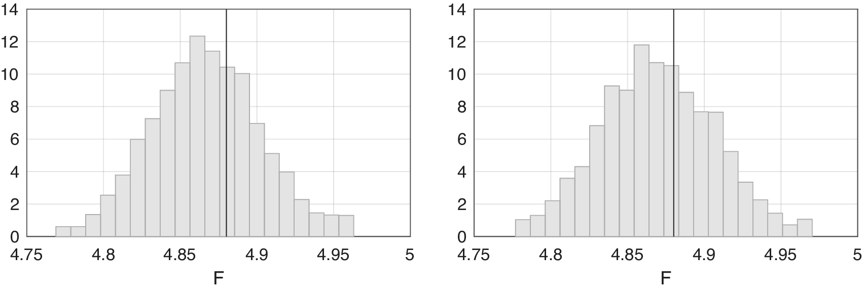
Figure 6. Posterior distributions over  $ F $ for the Lorenz ’96 case study. On the left, from conventional SMC $ {}^2 $, on the right, from SMC $ {}^2 $ with anytime moves, both running on the 128 GPU configuration.
Compute profiles for the runs are given in Figure 7, showing the busy and wait times of all processors involved in the computations. We see obvious wait time with conventional SMC $ {}^2 $, far more pronounced in the eight GPU cases, where a contesting process on one processor has encumbered the entire computation. The anytime move step grants a robustness to this contesting process, and wait times are significantly reduced. For the 128 GPU case, even in the absence of such exogenous problems, wait times are noticeably reduced.
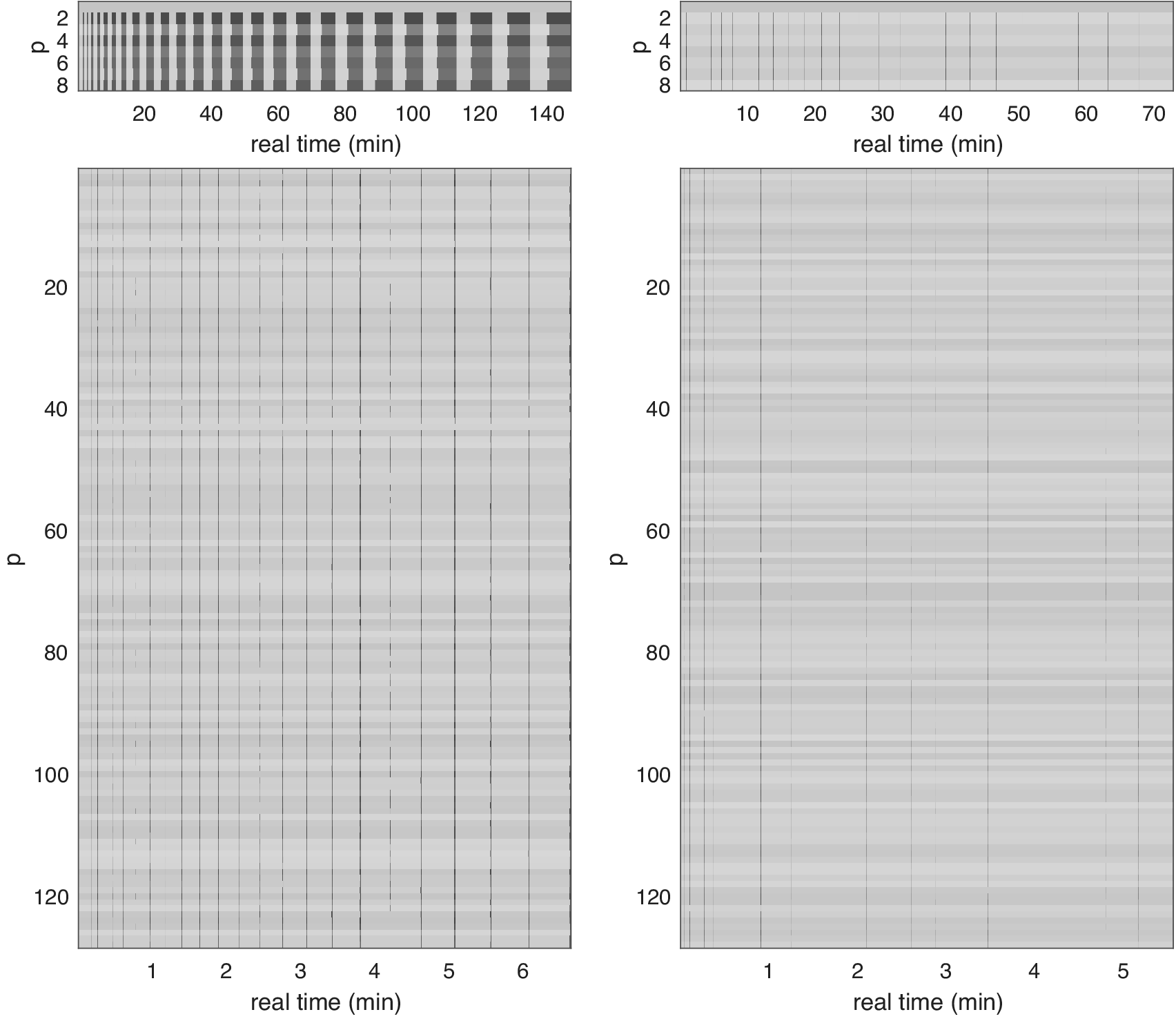
Figure 7. Compute profiles for the Lorenz ’96 case study. On the left is a conventional distributed SMC $ {}^2 $ method with a fixed number of moves per particle after resampling. On the right is distributed SMC $ {}^2 $ with anytime move steps. Each row represents the activity of a single processor over time: light gray while active and dark gray while waiting. The top profiles are for an eight GPU shared system where contesting processes are expected. The conventional method on the left exhibits significant idle time on processors 2–8 due to a contesting job on Processor 1. The two bottom profiles are for the 128 GPU configuration with no contesting processes. Wait time in the conventional methods on the left is significantly reduced in the anytime methods on the right.
5. Discussion
The framework presented is a generic means by which any MCMC algorithm—including iid sampling as a special case—can be made an anytime Monte Carlo algorithm. This facilitates the configuration of Monte Carlo computation in real-time terms, rather than in the number of simulations. The benefits of this have been demonstrated in a distributed computing context where, by setting real-time compute budgets, wait times are significantly reduced for an SMC algorithm that requires collective communication. The framework has potential applications elsewhere, for example as a foundation for real-time, fault-tolerant and energy-constrained Monte Carlo algorithms, for the management of cloud computing budgets, or for the fair computational comparison of methods.
We have assumed throughout that an algorithm is given to simulate the target distribution  $ \pi $, and that the anytime distribution $ \alpha $ is merely a consequence of this. The aim has then been to correct the length bias in $ \alpha $. This is a pragmatic approach, as it leverages existing Monte Carlo algorithms. A tantalizing alternative is to develop algorithms that, from the outset, yield $ \pi $ as the anytime distribution. This might be done with an underlying Markov chain that targets something other than $ \pi $ but that, by design, yields $ \pi $ once length biased. We expect, however, that to do this even approximately will require at least some knowledge of $ \tau $, which will restrict its applicability to specific cases only.
The proposed SMC method uses anytime move steps, but is not a complete anytime algorithm, as it does not provide control over the total compute budget. Its objective is to minimize the wait time that precedes resampling steps in a distributed implementation of SMC. On this account, it succeeds. A complete anytime SMC algorithm (of a conventional structure) will require, in addition, anytime weighting and anytime resampling steps, as well as the apportioning of the total compute budget between these. Because approximations may appear in each of these steps, the apportioning is not straightforward, and will involve tradeoffs. As already identified, for example, the redistribution of particles after resampling in a distributed environment is an expensive operation, and all or part of that time may be better invested in the budget allocation for anytime moves. Such investigations have been left to future work. An alternative means to an anytime SMC algorithm is to use a different structure to the conventional, as in the particle cascade (Paige et al., Reference Paige, Wood, Doucet and Teh2014). Whatever the structure, these anytime algorithms are somewhat more elaborate than the standard SMC algorithms for which theoretical results have been established, and may warrant further study.
Finally, we return to the strongest of the assumptions of the whole framework: that of the homogeneity of  $ \tau $ in time. This may be unrealistic in the presence of transient exogenous factors, such as intermittent network issues, or contesting processes running on the same hardware only temporarily. If the assumption is relaxed, so that $ \tau $ varies in time, the anytime distribution will vary as well, and ergodicity will not hold. Figure 4 suggests that, for example, an exogenous switching factor in $ \tau $ would induce transient effects in the anytime distribution that are not necessarily eliminated by the multiple chain strategy. There may be weaker assumptions under which comparable results and appropriate methods can be established, but this investigation is left to future work.
6. Conclusion
This work has presented an approach to allow any MCMC algorithm to be made an anytime Monte Carlo algorithm, eliminating the length bias associated with real-time budgets. This is particularly important in situations where the final state of a Markov chain is more important than computing averages over all states. It has applications in embedded, distributed, cloud, real-time, and fault-tolerant computing. To demonstrate the usefulness of the approach, a new SMC $ {}^2 $ method has been presented, which exhibits significantly reduced wait time when run on a large-scale distributed computing system.
Acknowledgments
The authors would like to thank the Isaac Newton Institute for Mathematical Sciences, Cambridge, for support and hospitality during the program Monte Carlo Methods for Complex Inference Problems (MCMW01), where some of this work was undertaken. This work was also financially supported by an EPSRC-Cambridge Big Data Travel Grant and EPSRC (EP/K020153/1), The Alan Turing Institute under the EPSRC grant EP/N510129/1, and the Swedish Foundation for Strategic Research (SSF) via the project ASSEMBLE. The authors would like to thank Pierre Jacob for helpful conversations.
Competing Interests
The authors declare no competing interests exist.
Data Availability Statement
The methods introduced in this paper are implemented in LibBi version 1.3.0, and the empirical results may be reproduced with the LibBi Anytime package. Both are available from www.libbi.org.
Author Contributions
Conceptualization, All; Methodology, All; Formal analysis, All; Data curation, L.M.M.; Writing-original draft, L.M.M. and S.S.S.; Writing–review & editing, All; Funding acquisition, All.
Supplementary Materials
To view supplementary material for this article, please visit http://dx.doi.org/10.1017/dce.2021.6.


 Open access
Comments
No Comments have been published for this article.