


1 Introduction
Given a finite, positive, and regular Borel measure, $\mu $
, on the complex unit circle,
$\mu $
, on the complex unit circle, $\partial \mathbb {D}$
, it is natural to consider its
$\partial \mathbb {D}$
, it is natural to consider its $L^2$
-space,
$L^2$
-space, $L^2 (\mu ) := L^2 (\mu , \partial \mathbb {D} )$
, as well as
$L^2 (\mu ) := L^2 (\mu , \partial \mathbb {D} )$
, as well as $H^2 (\mu ) := \mathbb {C} [ \zeta ] ^{-\| \cdot \| _{L^2(\mu )}}$
, the closure of the analytic polynomials,
$H^2 (\mu ) := \mathbb {C} [ \zeta ] ^{-\| \cdot \| _{L^2(\mu )}}$
, the closure of the analytic polynomials, $\mathbb {C} [\zeta ]$
, in
$\mathbb {C} [\zeta ]$
, in $L^2 (\mu )$
. The linear operator of multiplication by the independent variable,
$L^2 (\mu )$
. The linear operator of multiplication by the independent variable, $M^\mu _\zeta $
, is unitary on
$M^\mu _\zeta $
, is unitary on $L^2 (\mu )$
and has
$L^2 (\mu )$
and has $H^2 (\mu )$
as a closed invariant subspace so that
$H^2 (\mu )$
as a closed invariant subspace so that $Z^\mu := M^\mu _\zeta | _{H^2 (\mu )}$
is an isometry that will play a central role in our analysis. The
$Z^\mu := M^\mu _\zeta | _{H^2 (\mu )}$
is an isometry that will play a central role in our analysis. The $\mu $
-Cauchy transform of any
$\mu $
-Cauchy transform of any $h \in H^2 (\mu )$
is the analytic function,
$h \in H^2 (\mu )$
is the analytic function,
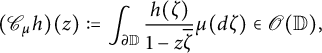 $$ \begin{align*}(\mathscr{C} _\mu h) (z) := \int _{\partial \mathbb{D}} \frac{h (\zeta)}{1- z \overline{\zeta}} \mu (d\zeta ) \in \mathscr{O} (\mathbb{D} ),\end{align*} $$
in the complex unit disk, $\mathbb {D} := (\mathbb {C} ) _1$
. Here, given a Banach space, X,
$\mathbb {D} := (\mathbb {C} ) _1$
. Here, given a Banach space, X, $(X) _1$
and
$(X) _1$
and $[X]_1$
denote its open and closed unit balls in the norm topology.
$[X]_1$
denote its open and closed unit balls in the norm topology.
Recall that a reproducing kernel Hilbert space (RKHS), $\mathcal {H}$
, is a Hilbert space of functions on a set, X, so that point evaluation at any point
$\mathcal {H}$
, is a Hilbert space of functions on a set, X, so that point evaluation at any point $x \in X$
yields a bounded linear functional on the space. The Riesz representation lemma then implies the existence of kernel vectors,
$x \in X$
yields a bounded linear functional on the space. The Riesz representation lemma then implies the existence of kernel vectors, $k_x$
,
$k_x$
, $x \in X$
, so that the bounded linear functional of point evaluation at x is implemented by inner products against
$x \in X$
, so that the bounded linear functional of point evaluation at x is implemented by inner products against $k_x$
. The function of two variables,
$k_x$
. The function of two variables, $k : X \times X \rightarrow \mathbb {C}$
,
$k : X \times X \rightarrow \mathbb {C}$
,
 $$ \begin{align*}k(x,y) := \left\langle {k_x} , {k_y} \right\rangle_{\mathcal{H}},\end{align*} $$
is then called the reproducing kernel of $\mathcal {H}$
. In this paper, all inner products and sesquilinear forms are conjugate linear in their first argument and linear in their second argument. Any reproducing kernel function is a positive kernel function on
$\mathcal {H}$
. In this paper, all inner products and sesquilinear forms are conjugate linear in their first argument and linear in their second argument. Any reproducing kernel function is a positive kernel function on $X \times X$
, i.e., for any finite set
$X \times X$
, i.e., for any finite set $\{ x_1, \dots , x_n \} \subseteq X$
, the
$\{ x_1, \dots , x_n \} \subseteq X$
, the $n \times n$
matrix,
$n \times n$
matrix,
 $$ \begin{align} [ k (x_i , x_j) ] _{1 \leq i,j \leq n} \geq 0, \end{align} $$
is positive semi-definite. Conversely, by a theorem of Aronszajn and Moore, given any positive kernel function, k, on $X \times X$
, one can construct a RKHS of functions on X with reproducing kernel k [Reference Aronszajn3] (see Section 2.2). Given this bijective correspondence between positive kernel functions on X and RKHS of functions on X, one writes
$X \times X$
, one can construct a RKHS of functions on X with reproducing kernel k [Reference Aronszajn3] (see Section 2.2). Given this bijective correspondence between positive kernel functions on X and RKHS of functions on X, one writes ${\mathcal {H} = \mathcal {H} (k)}$
if
${\mathcal {H} = \mathcal {H} (k)}$
if $\mathcal {H}$
is a RKHS with reproducing kernel k.
$\mathcal {H}$
is a RKHS with reproducing kernel k.
Equipping the vector space of $\mu $
-Cauchy transforms with the
$\mu $
-Cauchy transforms with the $H^2 (\mu )$
-inner product,
$H^2 (\mu )$
-inner product,
 $$ \begin{align*}\left\langle {\mathscr{C} _\mu g} , {\mathscr{C} _\mu h} \right\rangle_{\mu} := \left\langle {g} , {h} \right\rangle_{L^2 (\mu )}; \quad \quad g,h \in H^2 (\mu ),\end{align*} $$
yields a RKHS of analytic functions in $\mathbb {D}$
,
$\mathbb {D}$
, $\mathscr {H} ^+ ( \mu )$
, with reproducing kernel,
$\mathscr {H} ^+ ( \mu )$
, with reproducing kernel,
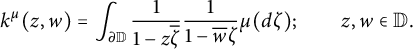 $$ \begin{align} k^\mu (z,w ) = \int _{\partial \mathbb{D}} \frac{1}{1-z \overline{\zeta}} \frac{1}{1-\overline{w}\zeta} \mu (d\zeta ); \quad \quad z,w \in \mathbb{D}. \end{align} $$
Using the above formula (1.2), it is easy to check that domination of measures implies domination of the reproducing kernels for their spaces of Cauchy transforms,
 $$ \begin{align*}\mu \leq t^2 \lambda , \ t>0 \quad \quad \Rightarrow \quad \quad k^\mu \leq t^2 k^\lambda\end{align*} $$
(see Theorem 4.1) where we write $k \leq K$
for positive kernel functions
$k \leq K$
for positive kernel functions $k,K$
on X, if
$k,K$
on X, if $K-k$
is a positive kernel function on X. We will say that
$K-k$
is a positive kernel function on X. We will say that $\lambda $
dominates
$\lambda $
dominates $\mu $
in the reproducing kernel sense (by
$\mu $
in the reproducing kernel sense (by $t^2>0$
) and write
$t^2>0$
) and write $\mu \leq _{RK} t^2 \lambda $
to denote that
$\mu \leq _{RK} t^2 \lambda $
to denote that $k^\mu \leq t^2 k^\lambda $
. By results of Aronszajn, domination of kernels,
$k^\mu \leq t^2 k^\lambda $
. By results of Aronszajn, domination of kernels, $k \leq t^2 K$
, is equivalent to bounded containment of their RKHS, i.e.,
$k \leq t^2 K$
, is equivalent to bounded containment of their RKHS, i.e., $k \leq t^2 K$
if and only if
$k \leq t^2 K$
if and only if $\mathcal {H} (k) \subseteq \mathcal {H} (K)$
and the norm of the linear embedding
$\mathcal {H} (k) \subseteq \mathcal {H} (K)$
and the norm of the linear embedding $\mathrm {e} : \mathcal {H} (k) \hookrightarrow \mathcal {H} (K)$
is at most
$\mathrm {e} : \mathcal {H} (k) \hookrightarrow \mathcal {H} (K)$
is at most $t>0$
[Reference Aronszajn3] (see Section 2.2 for a review of RKHS theory and these results). In summary, domination of measures implies bounded containment of their spaces of Cauchy transforms:
$t>0$
[Reference Aronszajn3] (see Section 2.2 for a review of RKHS theory and these results). In summary, domination of measures implies bounded containment of their spaces of Cauchy transforms:
 $$ \begin{align*}\mu \leq t^2 \lambda \quad \Rightarrow \quad \mathscr{H} ^+ (\mu ) \subseteq \mathscr{H} ^+ (\lambda ), \ \mathrm{e} _{\mu ,\lambda } : \mathscr{H} ^+ (\mu ) \hookrightarrow \mathscr{H} ^+ (\lambda ), \ \| \mathrm{e} _{\mu, \lambda } \| \leq t,\end{align*} $$
i.e., $\mu \leq t^2 \lambda \ \Rightarrow \ \mu \leq _{RK} t^2 \lambda $
.
$\mu \leq t^2 \lambda \ \Rightarrow \ \mu \leq _{RK} t^2 \lambda $
.
Building on this observation, we show that domination and, more generally, absolute continuity, as well as mutual singularity of measures can be completely characterized in terms of their spaces of Cauchy transforms. Moreover, we develop an independent construction of the Lebesgue decomposition and new proof of the Radon–Nikodym theorem using reproducing kernel methods and operator theory.
1.1 Outline
The following Background section, Section 2, provides an introduction to (i) the bijective correspondence between positive, finite, and regular Borel measures on the circle and contractive analytic functions in the disk, (ii) reproducing kernel theory, and (iii) the theory of densely-defined and positive semi-definite quadratic forms in a separable, complex Hilbert space.
Section 3 introduces the RKHSs, $\mathscr {H} ^+ (\mu )$
, of
$\mathscr {H} ^+ (\mu )$
, of $\mu $
-Cauchy transforms associated with any positive, finite, and regular Borel measure,
$\mu $
-Cauchy transforms associated with any positive, finite, and regular Borel measure, $\mu $
, on the complex unit circle. These are Hilbert spaces of holomorphic functions in the complex unit disk.
$\mu $
, on the complex unit circle. These are Hilbert spaces of holomorphic functions in the complex unit disk.
Our first main results appear in Section 4. Theorem 4.1 proves that domination of positive measures in the reproducing kernel sense is equivalent to domination in the classical sense:
Theorem 4.1 Given positive, finite, and regular Borel measures, $\mu $
and
$\mu $
and $\lambda $
on the unit circle,
$\lambda $
on the unit circle, $\mu \leq _{RK} t^2 \lambda $
for some
$\mu \leq _{RK} t^2 \lambda $
for some $t>0$
if and only if
$t>0$
if and only if $\mu \leq t^2 \lambda $
.
$\mu \leq t^2 \lambda $
.
This result is extended to general absolute continuity, written $\mu \ll \lambda $
, in Theorem 4.12. Namely, we say that
$\mu \ll \lambda $
, in Theorem 4.12. Namely, we say that $\mu $
is absolutely continuous in the reproducing kernel sense with respect to
$\mu $
is absolutely continuous in the reproducing kernel sense with respect to $\lambda $
, written
$\lambda $
, written $\mu \ll _{RK} \lambda $
, if the intersection of the space of
$\mu \ll _{RK} \lambda $
, if the intersection of the space of $\mu $
-Cauchy transforms with the space of
$\mu $
-Cauchy transforms with the space of $\lambda $
-Cauchy transforms,
$\lambda $
-Cauchy transforms, $\mathrm {int} (\mu , \lambda )$
, is norm-dense in
$\mathrm {int} (\mu , \lambda )$
, is norm-dense in $\mathscr {H} ^+ (\mu )$
.
$\mathscr {H} ^+ (\mu )$
.
Theorem 4.12 Let $\mu , \lambda $
be positive, finite, and regular Borel measures on
$\mu , \lambda $
be positive, finite, and regular Borel measures on $\partial \mathbb {D}$
. Then
$\partial \mathbb {D}$
. Then $\mu \ll \lambda $
if and only if
$\mu \ll \lambda $
if and only if $\mu \ll _{RK} \lambda $
.
$\mu \ll _{RK} \lambda $
.
Moreover, Theorem 4.12 gives a formula for the Radon–Nikodym derivative of $\mu $
with respect to
$\mu $
with respect to $\lambda $
in terms of the closed, densely-defined embedding,
$\lambda $
in terms of the closed, densely-defined embedding, $\mathrm {e} _{\mu , \lambda } : \mathrm {int} (\mu , \lambda ) := \mathscr {H} ^+ (\mu ) \cap \mathscr {H} ^+ (\lambda ) \subseteq \mathscr {H} ^+ (\mu ) \hookrightarrow \mathscr {H} ^+ (\lambda )$
.
$\mathrm {e} _{\mu , \lambda } : \mathrm {int} (\mu , \lambda ) := \mathscr {H} ^+ (\mu ) \cap \mathscr {H} ^+ (\lambda ) \subseteq \mathscr {H} ^+ (\mu ) \hookrightarrow \mathscr {H} ^+ (\lambda )$
.
These are satisfying results, however, actual construction of the Lebesgue decomposition of $\mu $
with respect to
$\mu $
with respect to $\lambda $
using reproducing kernel methods is more subtle and bifurcates into the two cases, where: The intersection space,
$\lambda $
using reproducing kernel methods is more subtle and bifurcates into the two cases, where: The intersection space, $\mathrm {int} (\mu , \lambda ) = \mathscr {H} ^+ (\mu ) \cap \mathscr {H} ^+ (\lambda )$
, of the spaces of
$\mathrm {int} (\mu , \lambda ) = \mathscr {H} ^+ (\mu ) \cap \mathscr {H} ^+ (\lambda )$
, of the spaces of $\mu $
and
$\mu $
and $\lambda $
-Cauchy transforms is (i) invariant, or, (ii) not invariant, for the image,
$\lambda $
-Cauchy transforms is (i) invariant, or, (ii) not invariant, for the image, $V^\mu $
, of
$V^\mu $
, of $Z^\mu = M^\mu _\zeta | _{H^2 (\mu )}$
under Cauchy transform. Some necessary and sufficient conditions for this to hold are obtained in Lemma 5.3 and Proposition 5.7. Namely, as described in Section 2.1, there is a bijection between contractive analytic functions in the complex unit disk and positive, finite, and regular Borel measures on the circle. If a positive measure,
$Z^\mu = M^\mu _\zeta | _{H^2 (\mu )}$
under Cauchy transform. Some necessary and sufficient conditions for this to hold are obtained in Lemma 5.3 and Proposition 5.7. Namely, as described in Section 2.1, there is a bijection between contractive analytic functions in the complex unit disk and positive, finite, and regular Borel measures on the circle. If a positive measure, $\mu $
, corresponds to an extreme point of this compact, convex set of contractive analytic functions, we say that
$\mu $
, corresponds to an extreme point of this compact, convex set of contractive analytic functions, we say that $\mu $
is extreme, otherwise
$\mu $
is extreme, otherwise $\mu $
is non-extreme. As established in Lemma 5.3 and Proposition 5.7, the intersection space,
$\mu $
is non-extreme. As established in Lemma 5.3 and Proposition 5.7, the intersection space, $\mathrm {int} (\mu , \lambda )$
will be
$\mathrm {int} (\mu , \lambda )$
will be $V_\mu $
-reducing if (i)
$V_\mu $
-reducing if (i) $\lambda $
is non-extreme or if (ii)
$\lambda $
is non-extreme or if (ii) $\mu +\lambda $
is extreme, and the intersection space will be nontrivial and not
$\mu +\lambda $
is extreme, and the intersection space will be nontrivial and not $V_\mu $
-invariant if
$V_\mu $
-invariant if $\mu , \lambda $
are both extreme but
$\mu , \lambda $
are both extreme but $\mu + \lambda $
is non-extreme.
$\mu + \lambda $
is non-extreme.
In the positive direction, we obtain the following:
Theorem 5.5 Let $\mu $
and
$\mu $
and $\lambda $
be finite, positive, and regular Borel measures on the unit circle. If the intersection space,
$\lambda $
be finite, positive, and regular Borel measures on the unit circle. If the intersection space, $\mathrm {int} (\mu , \lambda )$
is
$\mathrm {int} (\mu , \lambda )$
is $V_\mu $
-invariant and
$V_\mu $
-invariant and $\mu = \mu _{ac} + \mu _s$
is the Lebesgue decomposition of
$\mu = \mu _{ac} + \mu _s$
is the Lebesgue decomposition of $\mu $
with respect to
$\mu $
with respect to $\lambda $
, then
$\lambda $
, then
 $$ \begin{align*}\mathscr{H} ^+ (\mu ) = \mathscr{H} ^+ (\mu _{ac} ) \oplus \mathscr{H} ^+ (\mu _s).\end{align*} $$
In this case,
 $$ \begin{align*}\mathscr{H} ^+ (\mu _{ac} ) = \mathrm{int} (\mu , \lambda ) ^{-\| \cdot \| _\mu }, \quad \mbox{and} \quad \mathscr{H} ^+ (\mu _s ) \cap \mathscr{H} ^+ (\lambda ) = \{ 0 \}.\end{align*} $$
Given two positive, finite, and regular Borel measures, $\mu $
and
$\mu $
and $\lambda $
, on the complex unit circle,
$\lambda $
, on the complex unit circle, $\partial \mathbb {D}$
, one can associate with
$\partial \mathbb {D}$
, one can associate with $\mu $
a densely-defined and positive semi-definite sesquilinear or quadratic form in
$\mu $
a densely-defined and positive semi-definite sesquilinear or quadratic form in $H^2 (\lambda )$
. Namely, we define the form domain,
$H^2 (\lambda )$
. Namely, we define the form domain, $\mathrm {Dom} \, \mathfrak {q}_\mu \subseteq H^2 (\lambda )$
, as the disk algebra,
$\mathrm {Dom} \, \mathfrak {q}_\mu \subseteq H^2 (\lambda )$
, as the disk algebra, $\mathrm {Dom} \, \mathfrak {q} _\mu := A(\mathbb {D} )$
, the unital Banach algebra of all uniformly bounded analytic functions in the unit disk which extend continuously to the boundary, equipped with the supremum norm. The disk algebra embeds isometrically into the continuous functions on the circle,
$\mathrm {Dom} \, \mathfrak {q} _\mu := A(\mathbb {D} )$
, the unital Banach algebra of all uniformly bounded analytic functions in the unit disk which extend continuously to the boundary, equipped with the supremum norm. The disk algebra embeds isometrically into the continuous functions on the circle, $\mathscr {C} (\partial \mathbb {D} )$
and
$\mathscr {C} (\partial \mathbb {D} )$
and $A (\mathbb {D} )$
can be viewed as a dense subspace of
$A (\mathbb {D} )$
can be viewed as a dense subspace of $H^2 (\lambda )$
. The quadratic form,
$H^2 (\lambda )$
. The quadratic form, ${\mathfrak {q}_\mu : \mathrm {Dom} \, \mathfrak {q}_\mu \times \mathrm {Dom} \, \mathfrak {q}_\mu \rightarrow \mathbb {C}}$
is then defined in the obvious way by integration against
${\mathfrak {q}_\mu : \mathrm {Dom} \, \mathfrak {q}_\mu \times \mathrm {Dom} \, \mathfrak {q}_\mu \rightarrow \mathbb {C}}$
is then defined in the obvious way by integration against $\mu $
,
$\mu $
,
 $$ \begin{align} \mathfrak{q}_\mu (g, h) := \int _{\partial \mathbb{D}} \overline{g(\zeta )} h(\zeta) \mu (d\zeta ), \quad \quad g,h \in A (\mathbb{D} ) = \mathrm{Dom} \, \mathfrak{q} _\mu. \end{align} $$
As described in Section 4 and Theorem 4.8, there is a theory of Lebesgue decomposition of densely-defined and positive semi-definite quadratic forms in a Hilbert space, $\mathcal {H}$
. Namely, given any such form, there is a unique Simon–Lebesgue form decomposition,
$\mathcal {H}$
. Namely, given any such form, there is a unique Simon–Lebesgue form decomposition,
 $$ \begin{align*}\mathfrak{q}= \mathfrak{q}_{ac} + \mathfrak{q}_s,\end{align*} $$
where $0 \leq \mathfrak {q}_{ac}, \mathfrak {q}_s \leq \mathfrak {q}$
,
$0 \leq \mathfrak {q}_{ac}, \mathfrak {q}_s \leq \mathfrak {q}$
, $\mathfrak {q}_{ac}$
is absolutely continuous in the sense that it is closeable and it is maximal in the sense that
$\mathfrak {q}_{ac}$
is absolutely continuous in the sense that it is closeable and it is maximal in the sense that $\mathfrak {q}_{ac}$
is the largest closeable quadratic form bounded above by
$\mathfrak {q}_{ac}$
is the largest closeable quadratic form bounded above by $\mathfrak {q}$
. The form
$\mathfrak {q}$
. The form $\mathfrak {q}_s$
is singular in the sense that the only closeable positive semi-definite form it dominates is the identically
$\mathfrak {q}_s$
is singular in the sense that the only closeable positive semi-definite form it dominates is the identically $0$
form. Here, a positive semi-definite quadratic form,
$0$
form. Here, a positive semi-definite quadratic form, $\mathfrak {q}$
, with dense form domain
$\mathfrak {q}$
, with dense form domain $\mathrm {Dom} \, \mathfrak {q}$
in
$\mathrm {Dom} \, \mathfrak {q}$
in $\mathcal {H}$
, is closed, if
$\mathcal {H}$
, is closed, if $\mathrm {Dom} \, \mathfrak {q}$
is a Hilbert space, i.e., complete, with respect to the norm induced by the inner product
$\mathrm {Dom} \, \mathfrak {q}$
is a Hilbert space, i.e., complete, with respect to the norm induced by the inner product $\mathfrak {q} ( \cdot , \cdot ) + \left \langle {\cdot } , {\cdot } \right \rangle _{\mathcal {H}}$
. A form is then closeable if it has a closed extension (see Section 2.3 for an introduction to the theory of densely-defined and positive semi-definite quadratic forms).
$\mathfrak {q} ( \cdot , \cdot ) + \left \langle {\cdot } , {\cdot } \right \rangle _{\mathcal {H}}$
. A form is then closeable if it has a closed extension (see Section 2.3 for an introduction to the theory of densely-defined and positive semi-definite quadratic forms).
An immediate question is whether the Simon–Lebesgue decomposition of the form, $\mathfrak {q}_\mu $
, in
$\mathfrak {q}_\mu $
, in $H^2 (\lambda )$
coincides with the Lebesgue decomposition of
$H^2 (\lambda )$
coincides with the Lebesgue decomposition of $\mu $
with respect to
$\mu $
with respect to $\lambda $
. Namely, if
$\lambda $
. Namely, if $\mu = \mu _{ac} + \mu _s$
and
$\mu = \mu _{ac} + \mu _s$
and $\mathfrak {q}_\mu = \mathfrak {q}_{ac} + \mathfrak {q}_s$
, then is it true that
$\mathfrak {q}_\mu = \mathfrak {q}_{ac} + \mathfrak {q}_s$
, then is it true that $\mathfrak {q}_{ac} = \mathfrak {q}_{\mu _{ac}}$
and
$\mathfrak {q}_{ac} = \mathfrak {q}_{\mu _{ac}}$
and $\mathfrak {q}_s = \mathfrak {q}_{\mu _s}$
? A complete answer, summarized in the theorem below, is provided in Theorems 5.12 and 5.18 and Corollaries 5.14 and 5.15.
$\mathfrak {q}_s = \mathfrak {q}_{\mu _s}$
? A complete answer, summarized in the theorem below, is provided in Theorems 5.12 and 5.18 and Corollaries 5.14 and 5.15.
Theorem If $\mathfrak {q}_{\mu } = \mathfrak {q}_{ac} + \mathfrak {q}_s$
is the Simon–Lebesgue form decomposition of
$\mathfrak {q}_{\mu } = \mathfrak {q}_{ac} + \mathfrak {q}_s$
is the Simon–Lebesgue form decomposition of $\mathfrak {q}_\mu $
in
$\mathfrak {q}_\mu $
in $H^2 (\lambda )$
, then
$H^2 (\lambda )$
, then
 $$ \begin{align*}\mathscr{H} ^+ (\mu ) = \mathscr{H} ^+ (\mathfrak{q}_{ac} ) \oplus \mathscr{H} ^+ (\mathfrak{q} _s),\end{align*} $$
where
 $$ \begin{align*}\mathscr{H} ^+ (\mathfrak{q}_{ac} ) = \mathrm{int} (\mu , \lambda ) ^{-\| \cdot \|_\mu}.\end{align*} $$
If $\mu = \mu _{ac} + \mu _s$
is the Lebesgue decomposition of
$\mu = \mu _{ac} + \mu _s$
is the Lebesgue decomposition of $\mu $
with respect to
$\mu $
with respect to $\lambda $
, then
$\lambda $
, then
 $$ \begin{align*}\mathscr{H} ^+ (\mu ) = \mathscr{H} ^+ (\mu _{ac} ) + \mathscr{H} ^+ (\mu _s ),\end{align*} $$
is a complementary space decomposition in the sense of de Branges and Rovnyak, with $\mathscr {H} ^+ (\mu _{ac} )$
,
$\mathscr {H} ^+ (\mu _{ac} )$
, $\mathscr {H} ^+ (\mu _s)$
contractively contained in
$\mathscr {H} ^+ (\mu _s)$
contractively contained in $\mathscr {H} ^+ (\mu )$
. Moreover,
$\mathscr {H} ^+ (\mu )$
. Moreover, $\mathscr {H} ^+ (\mu _{ac} )$
is the largest RKHS,
$\mathscr {H} ^+ (\mu _{ac} )$
is the largest RKHS, $\mathcal {H} (k)$
, contractively contained in
$\mathcal {H} (k)$
, contractively contained in $\mathscr {H} ^+ (\mathfrak {q} _{ac} ) \subseteq \mathscr {H} ^+ (\mu )$
so that the closed embedding,
$\mathscr {H} ^+ (\mathfrak {q} _{ac} ) \subseteq \mathscr {H} ^+ (\mu )$
so that the closed embedding, $\mathrm {e} : \mathcal {H} (k) \cap \mathscr {H} ^+ (\lambda ) \subseteq \mathcal {H} (k) \hookrightarrow \mathscr {H} ^+ (\lambda )$
, is such that
$\mathrm {e} : \mathcal {H} (k) \cap \mathscr {H} ^+ (\lambda ) \subseteq \mathcal {H} (k) \hookrightarrow \mathscr {H} ^+ (\lambda )$
, is such that $\tau := \mathrm {e} \mathrm {e} ^*$
is Toeplitz for the image,
$\tau := \mathrm {e} \mathrm {e} ^*$
is Toeplitz for the image, $V^\lambda $
, of
$V^\lambda $
, of $Z^\lambda $
under Cauchy transform, i.e.,
$Z^\lambda $
under Cauchy transform, i.e., $V ^{\lambda *} \tau V ^\lambda = \tau $
. In particular, the Simon–Lebesgue decomposition of the quadratic form,
$V ^{\lambda *} \tau V ^\lambda = \tau $
. In particular, the Simon–Lebesgue decomposition of the quadratic form, $\mathfrak {q}_\mu $
, in
$\mathfrak {q}_\mu $
, in $H^2 (\lambda )$
coincides with the Lebesgue decomposition of
$H^2 (\lambda )$
coincides with the Lebesgue decomposition of $\mu $
with respect to
$\mu $
with respect to $\lambda $
if and only if
$\lambda $
if and only if $\mathrm {int} (\mu , \lambda )$
is
$\mathrm {int} (\mu , \lambda )$
is $V^\mu $
-invariant.
$V^\mu $
-invariant.
In the above, the spaces of $\mathfrak {q} _{ac}$
and
$\mathfrak {q} _{ac}$
and $\mathfrak {q} _s$
-Cauchy transforms are defined in an analogous way to the space of
$\mathfrak {q} _s$
-Cauchy transforms are defined in an analogous way to the space of $\mu $
-Cauchy transforms (see Section 5.1). By Proposition 5.7, the intersection space,
$\mu $
-Cauchy transforms (see Section 5.1). By Proposition 5.7, the intersection space, $\mathrm {int} (\mu , \lambda )$
, is not always
$\mathrm {int} (\mu , \lambda )$
, is not always $V^\mu $
-invariant. Example 5.9 (continued in Example 5.17) provides a concrete example, where
$V^\mu $
-invariant. Example 5.9 (continued in Example 5.17) provides a concrete example, where $\mu = m_+$
and
$\mu = m_+$
and $\lambda = m_-$
are the mutually singular restrictions of normalized Lebesgue measure, m, to the upper and lower half-circles, so that the Lebesgue decomposition of
$\lambda = m_-$
are the mutually singular restrictions of normalized Lebesgue measure, m, to the upper and lower half-circles, so that the Lebesgue decomposition of $m_+$
with respect to
$m_+$
with respect to $m_-$
has
$m_-$
has $m_{+; ac} =0$
but
$m_{+; ac} =0$
but $\mathrm {int} (m_+ ,m_-) \neq \{ 0 \}$
, so that
$\mathrm {int} (m_+ ,m_-) \neq \{ 0 \}$
, so that $\mathfrak {q} _{m_+; ac} \neq 0$
.
$\mathfrak {q} _{m_+; ac} \neq 0$
.
Remark This “reproducing kernel approach” to measure theory on the circle and Lebesgue decomposition of a positive measure with respect to Lebesgue measure was first considered and studied in [Reference Jury and Martin14, Reference Jury and Martin15], in a more general and noncommutative context.
2 Background
2.1 Function theory in the disk, measure theory on the circle
Classical analytic function theory in the complex unit disk and measure theory on the complex unit circle are fundamentally intertwined. There are bijective correspondences between (i) contractive analytic functions in the disk, (ii) analytic functions in the disk with positive semi-definite real part, i.e., Herglotz functions, and (iii) positive, finite, and regular Borel measures on the complex unit circle. Namely, starting with such a positive measure, $\mu $
, its Herglotz–Riesz transform is the Herglotz function,
$\mu $
, its Herglotz–Riesz transform is the Herglotz function,
 $$ \begin{align*}H _\mu (z) := \int _{\partial \mathbb{D}} \frac{1+z \overline{\zeta}}{1-z \overline{\zeta}} \mu (d\zeta ) \in \mathscr{O} (\mathbb{D} ).\end{align*} $$
It is easily verified that $\mathrm {Re} \, H_\mu (z) \geq 0$
, is a positive harmonic function. Applying the inverse Cayley transform to any Herglotz function, i.e., the Möbius transformation sending the open right half-plane onto the open unit disk,
$\mathrm {Re} \, H_\mu (z) \geq 0$
, is a positive harmonic function. Applying the inverse Cayley transform to any Herglotz function, i.e., the Möbius transformation sending the open right half-plane onto the open unit disk, $\mathbb {D}$
, which interchanges the points
$\mathbb {D}$
, which interchanges the points $1$
and
$1$
and $0$
, yields a contractive analytic function,
$0$
, yields a contractive analytic function, $b_\mu $
, in the disk,
$b_\mu $
, in the disk,
 $$ \begin{align*}b_\mu (z) := \frac{H_\mu (z) -1}{H_\mu (z) +1}, \quad \quad |b _\mu (z) | \leq 1, \ z \in \mathbb{D}.\end{align*} $$
(By the maximum modulus principle, $b_\mu $
is strictly contractive in
$b_\mu $
is strictly contractive in $\mathbb {D}$
unless it is constant.) Each of these transformations is essentially reversible. Namely, given any contractive analytic function, b, the Cayley transform,
$\mathbb {D}$
unless it is constant.) Each of these transformations is essentially reversible. Namely, given any contractive analytic function, b, the Cayley transform, $H_b := \frac {1 + b}{1-b}$
, is a Herglotz function and the Herglotz representation theorem states that if H is any Herglotz function in the disk, then there is a unique finite, positive, and regular Borel measure,
$H_b := \frac {1 + b}{1-b}$
, is a Herglotz function and the Herglotz representation theorem states that if H is any Herglotz function in the disk, then there is a unique finite, positive, and regular Borel measure, $\mu $
on the circle, so that
$\mu $
on the circle, so that
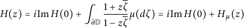 $$ \begin{align*}H (z) = i \mathrm{Im} \, H (0) + \int _{\partial \mathbb{D}} \frac{1+z \overline{\zeta}}{1-z \overline{\zeta}} \mu (d\zeta ) = i \mathrm{Im} \, H (0) + H_\mu (z)\end{align*} $$
(see [Reference Hoffman13, Boundary Values, Chapter 3]). To be precise, two Herglotz functions correspond to the same positive measure, $\mu $
, if and only if they differ by an imaginary constant. If
$\mu $
, if and only if they differ by an imaginary constant. If $H_1, H_2$
are two Herglotz functions so that
$H_1, H_2$
are two Herglotz functions so that $H_2 = H_1 + it$
for some
$H_2 = H_1 + it$
for some $t \in \mathbb {R}$
, then their corresponding inverse Cayley transforms obey
$t \in \mathbb {R}$
, then their corresponding inverse Cayley transforms obey
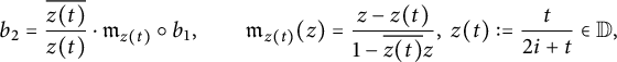 $$ \begin{align*}b _2 = \frac{\overline{z(t)}}{z(t)} \cdot \mathfrak{m} _{z(t)} \circ b_1, \quad \quad \mathfrak{m} _{z(t)} (z) = \frac{z - z(t)}{1-\overline{z(t)} z}, \ z(t) := \frac{t}{2i+t} \in \mathbb{D},\end{align*} $$
so that $b_2$
is, up to multiplication by the unimodular constant
$b_2$
is, up to multiplication by the unimodular constant $\frac {\overline {z(t)}}{z(t)}$
, a Möbius transformation,
$\frac {\overline {z(t)}}{z(t)}$
, a Möbius transformation, $\mathfrak {m} _{z(t)}$
, of
$\mathfrak {m} _{z(t)}$
, of $b_1$
, where
$b_1$
, where $\mathfrak {m} _{z(t)}$
defines an automorphism of the disk interchanging
$\mathfrak {m} _{z(t)}$
defines an automorphism of the disk interchanging $0$
with
$0$
with $z(t)$
.
$z(t)$
.
If a contractive analytic function, b, corresponds, essentially uniquely, to a positive measure, $\mu $
, in this way, we write
$\mu $
, in this way, we write $\mu := \mu _b$
, and
$\mu := \mu _b$
, and $\mu _b$
is called the Clark or Aleksandrov–Clark measure of b [Reference Clark5]. Many properties of contractive analytic functions in the disk can be described in terms of corresponding properties of their Clark measures and vice versa [Reference Aleksandrov2, Reference Aleksandrov1]. For example, by Fatou’s theorem, the Radon–Nikodym derivative of any Clark measure,
$\mu _b$
is called the Clark or Aleksandrov–Clark measure of b [Reference Clark5]. Many properties of contractive analytic functions in the disk can be described in terms of corresponding properties of their Clark measures and vice versa [Reference Aleksandrov2, Reference Aleksandrov1]. For example, by Fatou’s theorem, the Radon–Nikodym derivative of any Clark measure, $\mu _b$
, with respect to normalized Lebesgue measure, m, on the circle is given by the radial, or more generally non-tangential, limits of the real part of its Herglotz function,
$\mu _b$
, with respect to normalized Lebesgue measure, m, on the circle is given by the radial, or more generally non-tangential, limits of the real part of its Herglotz function,
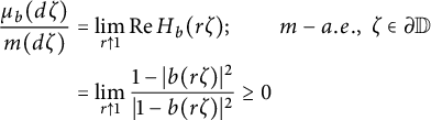 $$ \begin{align*} \frac{\mu _b (d\zeta )}{m(d\zeta )} & = \lim _{r \uparrow 1} \mathrm{Re} \, H_b (r\zeta ); \quad \quad m-a.e., \ \zeta \in \partial \mathbb{D} \\ & = \lim _{r \uparrow 1} \frac{ 1 - | b (r \zeta ) | ^2 }{| 1 - b (r \zeta )| ^2} \geq 0 \end{align*} $$
([Reference Fatou7], [Reference Hoffman13, Fatou’s Theorem, Chapter 3]). As a corollary of this formula, we see that b is inner, i.e., it has unimodular radial boundary limits m-a.e. on the circle, if and only if its Radon–Nikodym derivative vanishes almost everywhere, i.e., if and and only if its Clark measure is singular with respect to Lebesgue measure.
As a second example which will be relevant for our investigations here, b is an extreme point of the closed convex set of contractive analytic functions in the disk if and only if its Radon–Nikodym derivative with respect to Lebesgue measure is not log-integrable. That is, b is an extreme point if and only if
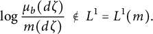 $$ \begin{align*}\mathrm{log} \, \frac{\mu _b (d\zeta )}{m (d\zeta)} \ \notin \ L^1 = L^1 (m).\end{align*} $$
This follows from the characterization of extreme points in the set of contractive analytic functions given in [Reference Hoffman13, Extreme Points, Chapter 9] and Fatou’s Radon–Nikodym formula as described above. Here, equipping the set of all bounded analytic functions in the disk with the supremum norm, we obtain the unital Banach algebra, $H^\infty $
, the Hardy algebra, whose closed unit ball,
$H^\infty $
, the Hardy algebra, whose closed unit ball, $[H^\infty ] _1$
, is the compact and convex set of contractive analytic functions in the disk. It further follows from a well-known theorem of Szegö (later strengthened by Kolmogoroff and Kreı̆n), that
$[H^\infty ] _1$
, is the compact and convex set of contractive analytic functions in the disk. It further follows from a well-known theorem of Szegö (later strengthened by Kolmogoroff and Kreı̆n), that $H^2 (\mu ) = L^2 (\mu )$
if and only if
$H^2 (\mu ) = L^2 (\mu )$
if and only if $\mu = \mu _b$
for an extreme point
$\mu = \mu _b$
for an extreme point $b \in [ H^\infty ] _1$
(see [Reference Hoffman13, Szegö’s Theorem, Chapter 4], [Reference Szegö23]). Namely, Szegö’s theorem gives a formula for the distance from the constant function
$b \in [ H^\infty ] _1$
(see [Reference Hoffman13, Szegö’s Theorem, Chapter 4], [Reference Szegö23]). Namely, Szegö’s theorem gives a formula for the distance from the constant function $1$
to the closure of the analytic polynomials with zero constant term in
$1$
to the closure of the analytic polynomials with zero constant term in $L^2 (\mu )$
:
$L^2 (\mu )$
:
 $$ \begin{align*}\mathrm{inf}_{\substack{p \in \mathbb{C} [\zeta ] \\ p(0) = 0}} \| 1 -p \| ^2 _{L^2 (\mu )} = \mathrm{exp} \, \int _{\partial \mathbb{D}} \mathrm{log} \, \frac{\mu (d\zeta )}{m (d\zeta)} \, m(d\zeta).\end{align*} $$
It follows, in particular, that b is an extreme point so that $\frac {d\mu }{dm}$
is not log-integrable if and only if
$\frac {d\mu }{dm}$
is not log-integrable if and only if $1$
belongs to the closure,
$1$
belongs to the closure, $H^2 _0 (\mu )$
, in
$H^2 _0 (\mu )$
, in $L^2 (\mu )$
of the analytic polynomials obeying
$L^2 (\mu )$
of the analytic polynomials obeying $p(0) =0$
. That is, if and only if
$p(0) =0$
. That is, if and only if $H^2 _0 (\mu ) = H^2 (\mu )$
. An inductive argument then shows that this is equivalent to
$H^2 _0 (\mu ) = H^2 (\mu )$
. An inductive argument then shows that this is equivalent to $H^2 (\mu ) = L^2 (\mu )$
, so that
$H^2 (\mu ) = L^2 (\mu )$
, so that $Z^\mu = M^\mu _\zeta | _{H^2 (\mu )} = M^\mu _\zeta $
is unitary. If
$Z^\mu = M^\mu _\zeta | _{H^2 (\mu )} = M^\mu _\zeta $
is unitary. If $\mu = \mu _b$
is the Clark measure of an extreme point, b, we will say that
$\mu = \mu _b$
is the Clark measure of an extreme point, b, we will say that $\mu $
is extreme, and that
$\mu $
is extreme, and that $\mu $
is non-extreme if b is not an extreme point.
$\mu $
is non-extreme if b is not an extreme point.
The results of this paper reinforce the close relationship between function theory in the disk and measure theory on the circle by establishing the Lebesgue decomposition and Radon–Nikodym theorem for positive measures using functional analysis and reproducing kernel theory applied to spaces of Cauchy transforms of positive measures. We will see that the reproducing kernel construction of the Lebesgue decomposition of a positive measure $\mu $
, with respect to another,
$\mu $
, with respect to another, $\lambda $
, bifurcates into the two cases, where: the intersection of the spaces of
$\lambda $
, bifurcates into the two cases, where: the intersection of the spaces of $\mu $
and
$\mu $
and $\lambda $
-Cauchy transforms, is (i) invariant, or (ii), not invariant for the image of
$\lambda $
-Cauchy transforms, is (i) invariant, or (ii), not invariant for the image of $Z ^\mu $
under Cauchy transform. Moreover, whether or not this intersection space is invariant is largely dependent on whether
$Z ^\mu $
under Cauchy transform. Moreover, whether or not this intersection space is invariant is largely dependent on whether $\lambda $
, or
$\lambda $
, or $\mu + \lambda $
are non-extreme or extreme.
$\mu + \lambda $
are non-extreme or extreme.
2.2 Reproducing kernel Hilbert spaces
As described in the introduction, a RKHS is any complex, separable Hilbert space of functions, $\mathcal {H}$
, on a set X, with the property that the linear functional of point evaluation at any
$\mathcal {H}$
, on a set X, with the property that the linear functional of point evaluation at any $x \in X$
is bounded on
$x \in X$
is bounded on $\mathcal {H}$
. Further, recall, as described above, that for any
$\mathcal {H}$
. Further, recall, as described above, that for any $x \in X$
, there is then a unique kernel vector or point evaluation vector,
$x \in X$
, there is then a unique kernel vector or point evaluation vector, $k_x \in \mathcal {H}$
so that
$k_x \in \mathcal {H}$
so that $\left \langle {k_x} , {h} \right \rangle _{\mathcal {H}} = h(x)$
for any
$\left \langle {k_x} , {h} \right \rangle _{\mathcal {H}} = h(x)$
for any $h \in \mathcal {H}$
and we write
$h \in \mathcal {H}$
and we write $\mathcal {H} = \mathcal {H} (k)$
, where
$\mathcal {H} = \mathcal {H} (k)$
, where $k : X \times X \rightarrow \mathbb {C}$
is a positive kernel function on X in the sense of Equation (1.1). Much of elementary RKHS theory was developed by N. Aronszajn in his seminal paper, [Reference Aronszajn3]. In particular, there is a bijective correspondence between RKHS on a set X and positive kernel functions on X given by the Aronszajn–Moore theorem, [Reference Aronszajn3, Part I], [Reference Paulsen and Raghupathi20, Proposition 2.13 and Theorem 2.14] and this motivates the notation
$k : X \times X \rightarrow \mathbb {C}$
is a positive kernel function on X in the sense of Equation (1.1). Much of elementary RKHS theory was developed by N. Aronszajn in his seminal paper, [Reference Aronszajn3]. In particular, there is a bijective correspondence between RKHS on a set X and positive kernel functions on X given by the Aronszajn–Moore theorem, [Reference Aronszajn3, Part I], [Reference Paulsen and Raghupathi20, Proposition 2.13 and Theorem 2.14] and this motivates the notation $\mathcal {H} = \mathcal {H} (k)$
.
$\mathcal {H} = \mathcal {H} (k)$
.
Theorem (Aronszajn–Moore)
If $\mathcal {H} = \mathcal {H} (k)$
is a RKHS of functions on a set, X, then k is a positive kernel function on X. Conversely, if k is a positive kernel function on X, then there is a (necessarily unique) RKHS of functions on X with reproducing kernel, k.
$\mathcal {H} = \mathcal {H} (k)$
is a RKHS of functions on a set, X, then k is a positive kernel function on X. Conversely, if k is a positive kernel function on X, then there is a (necessarily unique) RKHS of functions on X with reproducing kernel, k.
Any RKHS, $\mathcal {H} (k)$
, of functions on a set X, is naturally equipped with a multiplier algebra,
$\mathcal {H} (k)$
, of functions on a set X, is naturally equipped with a multiplier algebra, $\mathrm {Mult} (k)$
, the unital algebra of all functions on X which “multiply”
$\mathrm {Mult} (k)$
, the unital algebra of all functions on X which “multiply” $\mathcal {H} (k)$
into itself. That is,
$\mathcal {H} (k)$
into itself. That is, $g \in \mathrm {Mult} (k)$
if and only if
$g \in \mathrm {Mult} (k)$
if and only if $g\cdot h \in \mathcal {H} (k)$
for any
$g\cdot h \in \mathcal {H} (k)$
for any $h \in \mathcal {H} (k)$
. Any
$h \in \mathcal {H} (k)$
. Any $h \in \mathrm {Mult} (k)$
can be identified with the linear multiplication operator
$h \in \mathrm {Mult} (k)$
can be identified with the linear multiplication operator $M_h : \mathcal {H} (k) \rightarrow \mathcal {H} (k)$
. More generally, one can consider the set of multipliers,
$M_h : \mathcal {H} (k) \rightarrow \mathcal {H} (k)$
. More generally, one can consider the set of multipliers, $\mathrm {Mult} (k, K)$
, between two RKHS on the same set. If
$\mathrm {Mult} (k, K)$
, between two RKHS on the same set. If $h \in \mathrm {Mult} (k, K)$
, then
$h \in \mathrm {Mult} (k, K)$
, then $M_h$
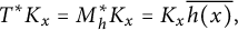
is always bounded, by the closed graph theorem. Adjoints of multiplication operators have a natural action on kernel vectors: If
$M_h$
is always bounded, by the closed graph theorem. Adjoints of multiplication operators have a natural action on kernel vectors: If $h \in \mathrm {Mult} (k , K)$
, then
$h \in \mathrm {Mult} (k , K)$
, then
 $$ \begin{align*}M_h ^* K_z = k_z \overline{h(z)}.\end{align*} $$
All RKHS in this paper will be RKHS, $\mathcal {H} (k)$
, of analytic functions in the complex unit disk,
$\mathcal {H} (k)$
, of analytic functions in the complex unit disk, $\mathbb {D} = (\mathbb {C} ) _1$
, with the additional property that evaluation of the Taylor coefficients of any
$\mathbb {D} = (\mathbb {C} ) _1$
, with the additional property that evaluation of the Taylor coefficients of any $h \in \mathcal {H} (k)$
(at
$h \in \mathcal {H} (k)$
(at $0$
) defines a bounded linear functional on
$0$
) defines a bounded linear functional on $\mathcal {H} (k)$
. Again, by the Riesz representation lemma, for any
$\mathcal {H} (k)$
. Again, by the Riesz representation lemma, for any $j \in \mathbb {N} \cup \{ 0 \}$
, there is then a unique Taylor coefficient kernel vector,
$j \in \mathbb {N} \cup \{ 0 \}$
, there is then a unique Taylor coefficient kernel vector, $k_j \in \mathcal {H} (k)$
, so that if
$k_j \in \mathcal {H} (k)$
, so that if $h \in \mathcal {H} (k)$
has Taylor series at
$h \in \mathcal {H} (k)$
has Taylor series at $0$
,
$0$
,
 $$ \begin{align*}h(z) = \sum _{j=0} ^\infty \hat{h} _j z^j,\end{align*} $$
then $\left \langle {k_j} , {h} \right \rangle _{\mathcal {H} (k)} = \hat {h} _j$
. It follows that
$\left \langle {k_j} , {h} \right \rangle _{\mathcal {H} (k)} = \hat {h} _j$
. It follows that
 $$ \begin{align*}\hat{k} (i , j) := \left\langle {k_i} , {k_j} \right\rangle_{\mathcal{H} (k)},\end{align*} $$
defines a positive kernel function, the coefficient reproducing kernel of $\mathcal {H} (k)$
, on the set
$\mathcal {H} (k)$
, on the set $\mathbb {N} \cup \{ 0 \}$
. It is easily checked that for any such Taylor coefficient RKHSs,
$\mathbb {N} \cup \{ 0 \}$
. It is easily checked that for any such Taylor coefficient RKHSs, $\mathcal {H} (k)$
and
$\mathcal {H} (k)$
and $\mathcal {H} (K)$
, of analytic functions in
$\mathcal {H} (K)$
, of analytic functions in $\mathbb {D}$
,
$\mathbb {D}$
,
 $$ \begin{align*}k \leq K \quad \Leftrightarrow \quad \hat{k} \leq \hat{K}.\end{align*} $$
The reproducing and coefficient reproducing kernels of a Taylor coefficient RKHS in $\mathbb {D}$
are related by the formulas:
$\mathbb {D}$
are related by the formulas:
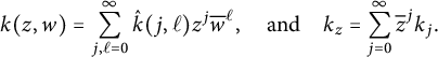 $$ \begin{align*}k(z,w) = \sum _{j,\ell =0} ^\infty \hat{k} (j , \ell) z^j \overline{w} ^\ell, \quad \mbox{and} \quad k_z = \sum _{j=0} ^\infty \overline{z} ^j k_j.\end{align*} $$
Adjoints of multipliers also have a natural convolution action on coefficient kernels, if $h \in \mathrm {Mult} (K , k)$
, then,
$h \in \mathrm {Mult} (K , k)$
, then,
 $$ \begin{align} M_h ^* K_\ell = \sum _{i+j = \ell} k_i \overline{\hat{h} _j}. \end{align} $$
We will say that a RKHS, $\mathcal {H} (k)$
, of analytic functions in
$\mathcal {H} (k)$
, of analytic functions in $X = \mathbb {D}$
is a coefficient RKHS in
$X = \mathbb {D}$
is a coefficient RKHS in $\mathbb {D}$
, if Taylor coefficient evaluations define bounded linear functionals on
$\mathbb {D}$
, if Taylor coefficient evaluations define bounded linear functionals on $\mathcal {H} (k)$
. In this case, the positive coefficient kernel function
$\mathcal {H} (k)$
. In this case, the positive coefficient kernel function $\hat {k}$
on
$\hat {k}$
on $\mathbb {N} \cup \{ 0 \}$
is an example of a discrete or formal reproducing kernel in the sense of [Reference Ball, Vinnikov and Alpay4].
$\mathbb {N} \cup \{ 0 \}$
is an example of a discrete or formal reproducing kernel in the sense of [Reference Ball, Vinnikov and Alpay4].
In this paper, it will be useful to consider densely-defined multipliers between RKHS $\mathcal {H} (K) , \mathcal {H} (k)$
on X, which are not necessarily bounded.
$\mathcal {H} (K) , \mathcal {H} (k)$
on X, which are not necessarily bounded.
Proposition 2.1 (Multipliers are closeable)
Let $k, K$
be positive kernel functions on X, and let h be a function on X so that the linear operator
$k, K$
be positive kernel functions on X, and let h be a function on X so that the linear operator $M_h : \mathrm {Dom} \, M_h \subseteq \mathcal {H} (k) \rightarrow \mathcal {H} (K)$
has dense domain,
$M_h : \mathrm {Dom} \, M_h \subseteq \mathcal {H} (k) \rightarrow \mathcal {H} (K)$
has dense domain, $\mathrm {Dom} \, M_h$
. Then
$\mathrm {Dom} \, M_h$
. Then $M_h$
is closeable, and closed on its maximal domain,
$M_h$
is closeable, and closed on its maximal domain, $\mathrm {Dom} _{\mathrm {max}} \, M_h := \{ g \in \mathcal {H} (k) | \ h \cdot g \in \mathcal {H} (K) \}$
,
$\mathrm {Dom} _{\mathrm {max}} \, M_h := \{ g \in \mathcal {H} (k) | \ h \cdot g \in \mathcal {H} (K) \}$
, $M_h ^* K_x = k_x \overline {h(x)}$
, and
$M_h ^* K_x = k_x \overline {h(x)}$
, and $\bigvee _{x \in X} K_x$
is a core for
$\bigvee _{x \in X} K_x$
is a core for $M_h ^*$
, if
$M_h ^*$
, if $M_h$
is defined on its maximal domain.
$M_h$
is defined on its maximal domain.
Recall that a linear operator with dense domain in a Hilbert space, $\mathcal {H}$
, is said to be closed if its graph is a closed subspace of
$\mathcal {H}$
, is said to be closed if its graph is a closed subspace of $\mathcal {H} \oplus \mathcal {H}$
. Further, recall that a dense set,
$\mathcal {H} \oplus \mathcal {H}$
. Further, recall that a dense set, $\mathscr {D} \subseteq \mathrm {Dom} \, A$
, contained in the domain of closed operator, A, is called a core for A if A is equal to the closure (minimal closed extension) of its restriction to
$\mathscr {D} \subseteq \mathrm {Dom} \, A$
, contained in the domain of closed operator, A, is called a core for A if A is equal to the closure (minimal closed extension) of its restriction to $\mathscr {D}$
. In general, given any two linear transformations
$\mathscr {D}$
. In general, given any two linear transformations $A, B$
, we say that B is an extension of A or that A is a restriction of B, written
$A, B$
, we say that B is an extension of A or that A is a restriction of B, written $A \subseteq B$
, if
$A \subseteq B$
, if $\mathrm {Dom} \, A \subseteq \mathrm {Dom} \, B$
and
$\mathrm {Dom} \, A \subseteq \mathrm {Dom} \, B$
and $B | _{\mathrm {Dom} \, A} = A$
. Equivalently, the set of all pairs
$B | _{\mathrm {Dom} \, A} = A$
. Equivalently, the set of all pairs $(x, Ax)$
, for
$(x, Ax)$
, for $x \in \mathscr {D}$
, is dense in the graph of A. Finally, A is closeable if it has a closed extension.
$x \in \mathscr {D}$
, is dense in the graph of A. Finally, A is closeable if it has a closed extension.
Proof Define $\mathrm {Dom} _{\mathrm {max}} \, M_h$
to be the linear space of all
$\mathrm {Dom} _{\mathrm {max}} \, M_h$
to be the linear space of all $g \in \mathcal {H} (k)$
so that
$g \in \mathcal {H} (k)$
so that $h \cdot g \in \mathcal {H} (K)$
. This is the largest domain on which
$h \cdot g \in \mathcal {H} (K)$
. This is the largest domain on which $M_h$
makes sense. If
$M_h$
makes sense. If $g_n \in \mathrm {Dom} _{\mathrm {max}} \, M_h$
is such that
$g_n \in \mathrm {Dom} _{\mathrm {max}} \, M_h$
is such that $g_n \rightarrow g$
and
$g_n \rightarrow g$
and $M_h g_n \rightarrow f$
, then since
$M_h g_n \rightarrow f$
, then since $\mathcal {H} (k) , \mathcal {H} (K)$
are RKHS, it necessarily follows that
$\mathcal {H} (k) , \mathcal {H} (K)$
are RKHS, it necessarily follows that
 $$ \begin{align*}g_n (x) \rightarrow g (x), \quad \mbox{and} \quad h(x) g_n (x) \rightarrow h(x) g(x) = f(x), \ x \in X.\end{align*} $$
This proves that $f = h \cdot g$
, so that
$f = h \cdot g$
, so that $g \in \mathrm {Dom} _{\mathrm {max}} \, M_h$
and
$g \in \mathrm {Dom} _{\mathrm {max}} \, M_h$
and $M_h$
is closed on
$M_h$
is closed on $\mathrm {Dom} _{\mathrm {max}} \, M_h$
. If
$\mathrm {Dom} _{\mathrm {max}} \, M_h$
. If $M_h$
is densely-defined on some other domain,
$M_h$
is densely-defined on some other domain, $\mathrm {Dom} \, M_h$
, then
$\mathrm {Dom} \, M_h$
, then $\mathrm {Dom} \, M_h \subseteq \mathrm {Dom} _{\mathrm {max}} \, M_h$
by maximality, so that
$\mathrm {Dom} \, M_h \subseteq \mathrm {Dom} _{\mathrm {max}} \, M_h$
by maximality, so that $M_h$
has a closed extension, and is hence closeable.
$M_h$
has a closed extension, and is hence closeable.
The fact that $\bigvee K_x$
is a core for
$\bigvee K_x$
is a core for $M_h ^*$
follows from the assumption that
$M_h ^*$
follows from the assumption that $M_h$
is defined (and closed) on its maximal domain. By maximality,
$M_h$
is defined (and closed) on its maximal domain. By maximality, $M_h$
, with domain
$M_h$
, with domain $\mathrm {Dom} _{\mathrm {max}} \, M_h$
, has no nontrivial closed extensions which act as multiplication by h. Let
$\mathrm {Dom} _{\mathrm {max}} \, M_h$
, has no nontrivial closed extensions which act as multiplication by h. Let $T_*$
be the closure of the restriction of
$T_*$
be the closure of the restriction of $M_h ^*$
to
$M_h ^*$
to $\bigvee K_x$
. Then
$\bigvee K_x$
. Then $T _* \subseteq M_h ^*$
is densely-defined and closed so that
$T _* \subseteq M_h ^*$
is densely-defined and closed so that $M_h \subseteq T:=T_* ^*$
, where
$M_h \subseteq T:=T_* ^*$
, where $T_* ^*$
, the adjoint of
$T_* ^*$
, the adjoint of $T_*$
is necessarily closed so that
$T_*$
is necessarily closed so that $T ^* = T_*$
. However,
$T ^* = T_*$
. However,
 $$ \begin{align*}T^* K_x = M_h ^* K_x = K_x \overline{h(x)},\end{align*} $$
so that T necessarily acts as multiplication by h on its domain. By maximality, $\mathrm {Dom} \, T = \mathrm {Dom} \, _{max} M_h$
and
$\mathrm {Dom} \, T = \mathrm {Dom} \, _{max} M_h$
and $M_h =T$
.
$M_h =T$
.
Remark 2.2 If $\mathcal {H} (k)$
and
$\mathcal {H} (k)$
and $\mathcal {H} (K)$
are Taylor coefficient RKHS in
$\mathcal {H} (K)$
are Taylor coefficient RKHS in $\mathbb {D}$
, then one can further show that the adjoint of any closed multiplication operator,
$\mathbb {D}$
, then one can further show that the adjoint of any closed multiplication operator, $M_h : \mathcal {H} (k) \rightarrow \mathcal {H} (K)$
acts as a convolution operator on coefficient kernels, as in Equation (2.1), and the linear span of all Taylor coefficient kernels is also a core for
$M_h : \mathcal {H} (k) \rightarrow \mathcal {H} (K)$
acts as a convolution operator on coefficient kernels, as in Equation (2.1), and the linear span of all Taylor coefficient kernels is also a core for $M_h ^*$
.
$M_h ^*$
.
One can define a natural partial order on positive kernel functions on a fixed set, X. Namely, if k and K are two positive kernel functions on the same set, X, we write $k \leq K$
, if
$k \leq K$
, if $K-k$
is a positive kernel function on X. Notice that the identically zero kernel function is a positive kernel on X, so that
$K-k$
is a positive kernel function on X. Notice that the identically zero kernel function is a positive kernel on X, so that $k \leq K$
can be equivalently written as
$k \leq K$
can be equivalently written as ${K- k \geq 0}$
. The following theorem of Aronszajn describes when one RKHS of functions on X is boundedly contained in another in terms of this partial order ([Reference Aronszajn3, Section 7], [Reference Paulsen and Raghupathi20, Theorem 5.1]).
${K- k \geq 0}$
. The following theorem of Aronszajn describes when one RKHS of functions on X is boundedly contained in another in terms of this partial order ([Reference Aronszajn3, Section 7], [Reference Paulsen and Raghupathi20, Theorem 5.1]).
Theorem (Aronszajn’s inclusion theorem)
Let $k, K$
be positive kernel functions on a set, X. Then
$k, K$
be positive kernel functions on a set, X. Then $\mathcal {H} (k) \subseteq \mathcal {H} (K)$
and the norm of the embedding
$\mathcal {H} (k) \subseteq \mathcal {H} (K)$
and the norm of the embedding $\mathrm {e} : \mathcal {H} (k ) \hookrightarrow \mathcal {H} (K)$
is at most
$\mathrm {e} : \mathcal {H} (k ) \hookrightarrow \mathcal {H} (K)$
is at most $t^2>0$
if and only if
$t^2>0$
if and only if $t^2 K \geq k$
.
$t^2 K \geq k$
.
If k and K are both positive kernel functions on a set, X, it is immediate that $k+K$
is also a positive kernel function on X. The following “sums of kernels” theorem of Aronszajn describes the norm of
$k+K$
is also a positive kernel function on X. The following “sums of kernels” theorem of Aronszajn describes the norm of $\mathcal {H} (k +K )$
and the decomposition of this space in terms of
$\mathcal {H} (k +K )$
and the decomposition of this space in terms of $\mathcal {H} (k)$
and
$\mathcal {H} (k)$
and $\mathcal {H} (K)$
(see [Reference Aronszajn3], [Reference Paulsen and Raghupathi20, Theorem 5.4 and Corollary 5.5]). Notice, in particular that
$\mathcal {H} (K)$
(see [Reference Aronszajn3], [Reference Paulsen and Raghupathi20, Theorem 5.4 and Corollary 5.5]). Notice, in particular that $k , K \leq k + K$
as kernel functions so that
$k , K \leq k + K$
as kernel functions so that $\mathcal {H} (k)$
and
$\mathcal {H} (k)$
and $\mathcal {H} (K)$
are contractively contained in
$\mathcal {H} (K)$
are contractively contained in $\mathcal {H} (k + K )$
, by the inclusion theorem.
$\mathcal {H} (k + K )$
, by the inclusion theorem.
Theorem (Aronszajn’s sums of kernels theorem)
Let $k, K$
be positive kernel functions on a set, X. Then,
$k, K$
be positive kernel functions on a set, X. Then, $\mathcal {H} (k+K) = \mathcal {H} (k) + \mathcal {H} (K)$
and
$\mathcal {H} (k+K) = \mathcal {H} (k) + \mathcal {H} (K)$
and
 $$ \begin{align*}\| h \| ^2 _{\mathcal{H} (k+K)} = \min \, \{ \| f \| ^2 _{\mathcal{H} (k)} + \| g \| ^2 _{\mathcal{H} (K)} | \ f + g = h \}.\end{align*} $$
In particular, $\mathcal {H} (k+ K) = \mathcal {H} (k) \oplus \mathcal {H} (K)$
if and only if
$\mathcal {H} (k+ K) = \mathcal {H} (k) \oplus \mathcal {H} (K)$
if and only if $\mathcal {H} (k) \cap \mathcal {H} (K) = \{ 0 \}$
.
$\mathcal {H} (k) \cap \mathcal {H} (K) = \{ 0 \}$
.
Observe that the sums of kernels theorem asserts that the algebraic sum $\mathcal {H} (k+K) = \mathcal {H} (k) + \mathcal {H} (K)$
is a direct sum if and only if it is an orthogonal direct sum. More can be said about this decomposition and the structure of
$\mathcal {H} (k+K) = \mathcal {H} (k) + \mathcal {H} (K)$
is a direct sum if and only if it is an orthogonal direct sum. More can be said about this decomposition and the structure of $\mathcal {H} (k+K)$
using the theory of operator-range spaces of contractions and their complementary spaces in the sense of de Branges and Rovnyak ([Reference de Branges and Rovnyak6], [Reference Fricain and Mashreghi8, Chapter 16]). Let
$\mathcal {H} (k+K)$
using the theory of operator-range spaces of contractions and their complementary spaces in the sense of de Branges and Rovnyak ([Reference de Branges and Rovnyak6], [Reference Fricain and Mashreghi8, Chapter 16]). Let $A \in \mathscr {L} (\mathcal {H} , \mathcal {J} )$
be a bounded linear operator. The operator-range space of A,
$A \in \mathscr {L} (\mathcal {H} , \mathcal {J} )$
be a bounded linear operator. The operator-range space of A, $\mathscr {R} (A)$
, is the Hilbert space obtained by equipping the range of A with the inner product that makes A a co-isometry onto its range. That is,
$\mathscr {R} (A)$
, is the Hilbert space obtained by equipping the range of A with the inner product that makes A a co-isometry onto its range. That is, $\mathscr {R} (A) = \mathrm {Ran} \, A \subseteq \mathcal {J} $
, with inner product,
$\mathscr {R} (A) = \mathrm {Ran} \, A \subseteq \mathcal {J} $
, with inner product,
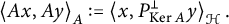 $$ \begin{align*}\left\langle {Ax} , {Ay} \right\rangle_A := \left\langle {x} , {P_{\mathrm{Ker} \, A} ^\perp y} \right\rangle_{\mathcal{H}}.\end{align*} $$
One can generally show that $\mathscr {R} (A) = \mathscr {R} ( \sqrt {A A^*} )$
([Reference Fricain and Mashreghi8, Corollary 16.8]). If A is a contraction,
$\mathscr {R} (A) = \mathscr {R} ( \sqrt {A A^*} )$
([Reference Fricain and Mashreghi8, Corollary 16.8]). If A is a contraction, $\| A \| \leq 1$
, then
$\| A \| \leq 1$
, then $\mathscr {R} (A) \subseteq \mathcal {J} $
is contractively contained in
$\mathscr {R} (A) \subseteq \mathcal {J} $
is contractively contained in $\mathcal {J} $
in the sense that the embedding,
$\mathcal {J} $
in the sense that the embedding, $\mathrm {e} : \mathscr {R} (A) \hookrightarrow \mathcal {J} $
is a linear contraction. In this case, one can define the complementary space of A,
$\mathrm {e} : \mathscr {R} (A) \hookrightarrow \mathcal {J} $
is a linear contraction. In this case, one can define the complementary space of A, $\mathscr {R} ^c (A) := \mathscr {R} (\sqrt {I-AA^*} )$
. The notion of complementary space was originally introduced in a more geometric way by de Branges and Rovnyak [Reference de Branges and Rovnyak6]. Namely, if
$\mathscr {R} ^c (A) := \mathscr {R} (\sqrt {I-AA^*} )$
. The notion of complementary space was originally introduced in a more geometric way by de Branges and Rovnyak [Reference de Branges and Rovnyak6]. Namely, if $\mathcal {H}$
is any Hilbert space and
$\mathcal {H}$
is any Hilbert space and $\mathscr {R} \subseteq \mathcal {H}$
is a Hilbert space which is contractively contained in
$\mathscr {R} \subseteq \mathcal {H}$
is a Hilbert space which is contractively contained in $\mathcal {H}$
, then
$\mathcal {H}$
, then $\mathscr {R} = \mathscr {R} (\mathrm {j} )$
, where
$\mathscr {R} = \mathscr {R} (\mathrm {j} )$
, where $\mathrm {j} : \mathscr {R} \hookrightarrow \mathcal {H}$
is the contractive embedding. L. de Branges and J. Rovnyak defined the complementary space,
$\mathrm {j} : \mathscr {R} \hookrightarrow \mathcal {H}$
is the contractive embedding. L. de Branges and J. Rovnyak defined the complementary space, $\mathscr {R} ^c$
of
$\mathscr {R} ^c$
of $\mathscr {R}$
as the set of all
$\mathscr {R}$
as the set of all $y \in \mathcal {H}$
so that
$y \in \mathcal {H}$
so that
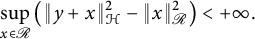 $$ \begin{align*}\sup _{x \in \mathscr{R}} \left( \| y + x \| _{\mathcal{H}} ^2 - \| x \| ^2 _{\mathscr{R}} \right) < + \infty.\end{align*} $$
One can prove that $\mathscr {R} ^c = \mathscr {R} ^c (\mathrm {j} )$
and that the above formula is equal to the norm of y in
$\mathscr {R} ^c = \mathscr {R} ^c (\mathrm {j} )$
and that the above formula is equal to the norm of y in $\mathscr {R} ^c (\mathrm {j})$
, so that these two definitions coincide [Reference Fricain and Mashreghi8, Chapter 16]. The following theorem summarizes several results in the theory of operator-range spaces (see [Reference Fricain and Mashreghi8, Chapter 16]).
$\mathscr {R} ^c (\mathrm {j})$
, so that these two definitions coincide [Reference Fricain and Mashreghi8, Chapter 16]. The following theorem summarizes several results in the theory of operator-range spaces (see [Reference Fricain and Mashreghi8, Chapter 16]).
Theorem 2.3 (Operator-range spaces of contractions)
Let $A \in \mathscr {L} ( \mathcal {H} , \mathcal {J} )$
be a contraction. If
$A \in \mathscr {L} ( \mathcal {H} , \mathcal {J} )$
be a contraction. If $\mathrm {e} : \mathscr {R} (A) \hookrightarrow \mathcal {J} $
and
$\mathrm {e} : \mathscr {R} (A) \hookrightarrow \mathcal {J} $
and $\mathrm {j} : \mathscr {R} ^c (A) \hookrightarrow \mathcal {J} $
are the contractive embeddings, then
$\mathrm {j} : \mathscr {R} ^c (A) \hookrightarrow \mathcal {J} $
are the contractive embeddings, then
 $$ \begin{align*}\mathcal{J} = \mathscr{R} (A) + \mathscr{R} ^c (A).\end{align*} $$
For any $x = y + z \in \mathcal {J} $
so that
$x = y + z \in \mathcal {J} $
so that $y \in \mathscr {R} (A)$
and
$y \in \mathscr {R} (A)$
and $z \in \mathscr {R} ^c (A)$
, the Pythagorean equality,
$z \in \mathscr {R} ^c (A)$
, the Pythagorean equality,
 $$ \begin{align} \| x \| ^2 _{\mathcal{J} } = \| y \| ^2 _{\mathscr{R} (A)} + \| z \| ^2 _{\mathscr{R} ^c (A)}, \end{align} $$
holds if and only if $y = \mathrm {e} \mathrm {e} ^* x$
and
$y = \mathrm {e} \mathrm {e} ^* x$
and $z= \mathrm {j} \mathrm {j} ^*x$
, so that, in particular,
$z= \mathrm {j} \mathrm {j} ^*x$
, so that, in particular, $I _{\mathcal {J}} = \mathrm {e} \mathrm {e} ^* + \mathrm {j} \mathrm {j} ^*$
. As a vector space, the overlapping space is
$I _{\mathcal {J}} = \mathrm {e} \mathrm {e} ^* + \mathrm {j} \mathrm {j} ^*$
. As a vector space, the overlapping space is
 $$ \begin{align*}\mathscr{R} (A) \cap \mathscr{R} ^c (A) = A \mathscr{R} ^c (A^*),\end{align*} $$
and $A : \mathscr {R} ^c (A^*) \rightarrow \mathscr {R} ^c (A)$
acts as a linear contraction.
$A : \mathscr {R} ^c (A^*) \rightarrow \mathscr {R} ^c (A)$
acts as a linear contraction.
Moreover, the following are equivalent:
-
(i) A is a partial isometry,
-
(ii) $\mathscr {R} (A)$
and
$\mathscr {R} ^c (A)$
are isometrically contained in
$\mathcal {J} $
as orthogonal complements,
$\mathcal {J} = \mathscr {R} (A) \oplus \mathscr {R} ^c (A)$
,
$\mathscr {R} (A)$
and
$\mathscr {R} ^c (A)$
are isometrically contained in
$\mathcal {J} $
as orthogonal complements,
$\mathcal {J} = \mathscr {R} (A) \oplus \mathscr {R} ^c (A)$
, -
(iii)
$\mathscr {R} (A) \cap \mathscr {R} ^c (A) = \{ 0 \}$
.


Observe that, as in Aronszajn’s sums of kernels theorem, the algebraic sum $\mathcal {J} = \mathscr {R} (A) + \mathscr {R} ^c (A)$
is a direct sum if and only if it is an orthogonal direct sum.
$\mathcal {J} = \mathscr {R} (A) + \mathscr {R} ^c (A)$
is a direct sum if and only if it is an orthogonal direct sum.
Theorem 2.4 Let $\mathcal {H} (K)$
be a RKHS on a set, X. If
$\mathcal {H} (K)$
be a RKHS on a set, X. If $\mathcal {H} (k)$
is another RKHS on X which embeds, contractively, in
$\mathcal {H} (k)$
is another RKHS on X which embeds, contractively, in $\mathcal {H} (K)$
, and
$\mathcal {H} (K)$
, and $\mathrm {e} : \mathcal {H} (k) \hookrightarrow \mathcal {H} (K)$
is the contractive embedding, then
$\mathrm {e} : \mathcal {H} (k) \hookrightarrow \mathcal {H} (K)$
is the contractive embedding, then $\mathcal {H} (k) = \mathscr {R} (\mathrm {e} )$
and the complementary space,
$\mathcal {H} (k) = \mathscr {R} (\mathrm {e} )$
and the complementary space, $\mathscr {R} ^c (\mathrm {e} )$
, is the RKHS on X with reproducing kernel
$\mathscr {R} ^c (\mathrm {e} )$
, is the RKHS on X with reproducing kernel $K-k$
.
$K-k$
.
An embedding of RKHS, $\mathrm {e}: \mathcal {H} (k) \hookrightarrow \mathcal {H} (K)$
, is necessarily injective.
$\mathrm {e}: \mathcal {H} (k) \hookrightarrow \mathcal {H} (K)$
, is necessarily injective.
Proof Let $\mathrm {e} : \mathcal {H} (k) \hookrightarrow \mathcal {H} (K)$
be the contractive embedding and consider the operator-range space of
$\mathrm {e} : \mathcal {H} (k) \hookrightarrow \mathcal {H} (K)$
be the contractive embedding and consider the operator-range space of $\mathrm {e}$
. Given any
$\mathrm {e}$
. Given any $g,h \in \mathcal {H} (k)$
, we have that
$g,h \in \mathcal {H} (k)$
, we have that
 $$ \begin{align*}\left\langle {\mathrm{e} g} , {\mathrm{e} h} \right\rangle_{\mathrm{e}} = \left\langle {g} , {h} \right\rangle_{\mathcal{H} (k)},\end{align*} $$
since $\mathrm {e}$
is injective. Hence, for any
$\mathrm {e}$
is injective. Hence, for any $x \in X$
,
$x \in X$
,
 $$ \begin{align} \left\langle {\mathrm{e} k _x} , {\mathrm{e}h} \right\rangle_{\mathrm{e}} = \left\langle {k _x} , {h} \right\rangle_{\mathcal{H} (k)} = h (x) = (\mathrm{e} h ) (x), \end{align} $$
and it follows that $\mathscr {R} (\mathrm {e} ) = \mathcal {H} (k)$
. Indeed, equation (2.3) shows that
$\mathscr {R} (\mathrm {e} ) = \mathcal {H} (k)$
. Indeed, equation (2.3) shows that $\mathscr {R} (\mathrm {e} )$
is a RKHS on X with point evaluation vectors
$\mathscr {R} (\mathrm {e} )$
is a RKHS on X with point evaluation vectors $\widetilde {k} _x := \mathrm {e} k_x$
and that for any
$\widetilde {k} _x := \mathrm {e} k_x$
and that for any $x,y \in X$
,
$x,y \in X$
,
 $$ \begin{align*}\widetilde{k} (x,y) = \left\langle {\widetilde{k} _x} , {\widetilde{k} _y} \right\rangle_{\mathrm{e}} = \left\langle {k_x} , {k_y} \right\rangle = k(x,y),\end{align*} $$
so that $\mathscr {R} (\mathrm {e} ) = \mathcal {H} (\widetilde {k} ) = \mathcal {H} (k)$
. Now consider the complementary space,
$\mathscr {R} (\mathrm {e} ) = \mathcal {H} (\widetilde {k} ) = \mathcal {H} (k)$
. Now consider the complementary space, $\mathscr {R} ^c (\mathrm {e} )$
, of
$\mathscr {R} ^c (\mathrm {e} )$
, of $\mathcal {H} (k)= \mathscr {R} (\mathrm {e} )$
. Since this complementary space is contractively contained in
$\mathcal {H} (k)= \mathscr {R} (\mathrm {e} )$
. Since this complementary space is contractively contained in $\mathcal {H} (K)$
, for any
$\mathcal {H} (K)$
, for any $\sqrt {I - \mathrm {e} \mathrm {e} ^*} g \in \mathscr {R} ^c (\mathrm {e} )$
,
$\sqrt {I - \mathrm {e} \mathrm {e} ^*} g \in \mathscr {R} ^c (\mathrm {e} )$
,
 $$ \begin{align*} \left\langle {(I - \mathrm{e} \mathrm{e} ^*) K_x} , {\sqrt{I - \mathrm{e} \mathrm{e} ^*} g} \right\rangle_{\mathscr{H}} & = \left\langle {\sqrt{I - \mathrm{e} \mathrm{e} ^*} K_x} , {g} \right\rangle_{\mathcal{H} (K)} \\& = ( \sqrt{I - \mathrm{e} \mathrm{e} ^*} g ) (x), \end{align*} $$
proving that $\mathscr {R} ^c (\mathrm {e})$
is also a RKHS on X with point evaluation vectors
$\mathscr {R} ^c (\mathrm {e})$
is also a RKHS on X with point evaluation vectors $k ' _x := ( I - \mathrm {e} \mathrm {e} ^* ) K _x$
. Hence,
$k ' _x := ( I - \mathrm {e} \mathrm {e} ^* ) K _x$
. Hence,
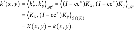 $$ \begin{align*} k'(x,y) & = \left\langle {k' _x} , {k ' _y} \right\rangle_{\mathscr{H}} = \left\langle {( I - \mathrm{e} \mathrm{e} ^* ) K_x } , {( I - \mathrm{e} \mathrm{e} ^* ) K_y} \right\rangle_{\mathscr{H}} \\ & = \left\langle {K_x} , {(I - \mathrm{e} \mathrm{e} ^*) K_y} \right\rangle_{\mathcal{H} (K)} \\ & = K (x,y) - k (x,y). \end{align*} $$
If $\mathrm {j} : \mathscr {R} ^c (\mathrm {e}) \hookrightarrow \mathscr {H} ^+ (\mu )$
is the contractive embedding, then observe that
$\mathrm {j} : \mathscr {R} ^c (\mathrm {e}) \hookrightarrow \mathscr {H} ^+ (\mu )$
is the contractive embedding, then observe that $\mathrm {j} \mathrm {j} ^* + \mathrm {e} \mathrm {e} ^* = I_{\mathcal {H} (K)}$
, so that
$\mathrm {j} \mathrm {j} ^* + \mathrm {e} \mathrm {e} ^* = I_{\mathcal {H} (K)}$
, so that
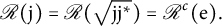 $$ \begin{align*}\mathscr{R} (\mathrm{j} ) = \mathscr{R} (\sqrt{\mathrm{j} \mathrm{j} ^*} ) = \mathscr{R} ^c (\mathrm{e} ).\\[-34pt] \end{align*} $$
The previous theorem and Theorem 2.3 provide additional information on the structure and decomposition of $\mathcal {H} (k +K)$
in Aronszajn’s sums of kernels theorem.
$\mathcal {H} (k +K)$
in Aronszajn’s sums of kernels theorem.
Corollary 2.5 Let $k,K$
be positive kernel functions on a set, X, and let
$k,K$
be positive kernel functions on a set, X, and let $\mathrm {e} : \mathcal {H} (k) \hookrightarrow \mathcal {H} (k+K)$
and
$\mathrm {e} : \mathcal {H} (k) \hookrightarrow \mathcal {H} (k+K)$
and $\mathrm {j} : \mathcal {H} (K) \hookrightarrow \mathcal {H} (k+K)$
be the contractive embeddings. Then we can identify
$\mathrm {j} : \mathcal {H} (K) \hookrightarrow \mathcal {H} (k+K)$
be the contractive embeddings. Then we can identify $\mathcal {H} (k)$
and
$\mathcal {H} (k)$
and $\mathcal {H} (K)$
with the operator range spaces
$\mathcal {H} (K)$
with the operator range spaces $\mathscr {R} (\mathrm {e} )$
and
$\mathscr {R} (\mathrm {e} )$
and $\mathscr {R} (\mathrm {j})$
, respectively. Moreover,
$\mathscr {R} (\mathrm {j})$
, respectively. Moreover, $I_{\mathcal {H} (k+K)} = \mathrm {e} \mathrm {e} ^* + \mathrm {j} \mathrm {j} ^*$
so that
$I_{\mathcal {H} (k+K)} = \mathrm {e} \mathrm {e} ^* + \mathrm {j} \mathrm {j} ^*$
so that $\mathcal {H} (K) = \mathscr {R} ^c (\mathrm {e} )$
is the complementary space of
$\mathcal {H} (K) = \mathscr {R} ^c (\mathrm {e} )$
is the complementary space of $\mathscr {R} (\mathrm {e} ) = \mathcal {H} (k)$
, and given any
$\mathscr {R} (\mathrm {e} ) = \mathcal {H} (k)$
, and given any $h \in \mathcal {H} (k + K)$
,
$h \in \mathcal {H} (k + K)$
,
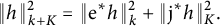 $$ \begin{align*}\| h \|_{k+K} ^2 = \| \mathrm{e} ^* h \| _k ^2 + \| \mathrm{j} ^* h \| ^2 _K.\end{align*} $$
The intersection space, $\mathcal {H} (k) \cap \mathcal {H} (K)$
is equal to
$\mathcal {H} (k) \cap \mathcal {H} (K)$
is equal to $\mathrm {e} \mathscr {R} ^c (\mathrm {e} ^*)$
and
$\mathrm {e} \mathscr {R} ^c (\mathrm {e} ^*)$
and $\mathrm {j} \mathscr {R} ^c (\mathrm {j} ^* )$
, and
$\mathrm {j} \mathscr {R} ^c (\mathrm {j} ^* )$
, and $\mathrm {e} : \mathscr {R} ^c (\mathrm {e} ^*) \rightarrow \mathscr {R} ^c (\mathrm {e} ) = \mathcal {H} (K)$
,
$\mathrm {e} : \mathscr {R} ^c (\mathrm {e} ^*) \rightarrow \mathscr {R} ^c (\mathrm {e} ) = \mathcal {H} (K)$
, $\mathrm {j} : \mathscr {R} ^c (\mathrm {j} ^* ) \rightarrow \mathscr {R} ^c (\mathrm {j})$
are contractions.
$\mathrm {j} : \mathscr {R} ^c (\mathrm {j} ^* ) \rightarrow \mathscr {R} ^c (\mathrm {j})$
are contractions.
Finally, as described in [Reference Okutmustur and Gheondea18] and [Reference Martin and Shamovich17, Section 5], we can define a pair of natural “lattice operations,” $\vee $
and
$\vee $
and $\wedge $
on the set of all positive kernel functions on a fixed set, X. Given two positive kernel functions, k and K, on X, let
$\wedge $
on the set of all positive kernel functions on a fixed set, X. Given two positive kernel functions, k and K, on X, let $k\vee K := k + K$
, a positive kernel function on X. We can also construct a second RKHS on X by defining
$k\vee K := k + K$
, a positive kernel function on X. We can also construct a second RKHS on X by defining
 $$ \begin{align*}\mathrm{int} (k , K) := \mathcal{H} (k ) \cap \mathcal{H} (K),\end{align*} $$
equipped with the inner product
 $$ \begin{align*}\left\langle {g} , {h} \right\rangle_{k \wedge K} := \left\langle {g} , {h} \right\rangle_k + \left\langle {g} , {h} \right\rangle_K.\end{align*} $$
It is not difficult to verify that $\mathrm {int} (k,K)$
, equipped with this inner product is complete, and that point evaluation at any
$\mathrm {int} (k,K)$
, equipped with this inner product is complete, and that point evaluation at any $x \in X$
defines a bounded linear functional on
$x \in X$
defines a bounded linear functional on $\mathrm {int} (k, K)$
, so that this is a RKHS,
$\mathrm {int} (k, K)$
, so that this is a RKHS, $\mathcal {H} (k \wedge K)$
, of functions on X. The following theorem describes a useful relationship between
$\mathcal {H} (k \wedge K)$
, of functions on X. The following theorem describes a useful relationship between $\mathcal {H} (k + K)$
and
$\mathcal {H} (k + K)$
and $\mathcal {H} (k \wedge K)$
(see [Reference Martin and Shamovich17, Theorem 5.2], [Reference Okutmustur and Gheondea18]).
$\mathcal {H} (k \wedge K)$
(see [Reference Martin and Shamovich17, Theorem 5.2], [Reference Okutmustur and Gheondea18]).
Theorem (Sums and intersections of RKHS)
Let $k, K \geq 0$
be positive kernel functions on a set, X. Define two linear maps,
$k, K \geq 0$
be positive kernel functions on a set, X. Define two linear maps, $U_\vee $
and
$U_\vee $
and $U_\wedge $
of
$U_\wedge $
of $\mathcal {H} (k + K)$
and
$\mathcal {H} (k + K)$
and $\mathcal {H} (k\wedge K)$
, respectively, into
$\mathcal {H} (k\wedge K)$
, respectively, into $\mathcal {H} (k) \oplus \mathcal {H} (K)$
by
$\mathcal {H} (k) \oplus \mathcal {H} (K)$
by
 $$ \begin{align*}U_\vee (k +K )_x := k_x \oplus K_x, \ x \in X, \quad \mbox{and} \quad U_\wedge f := f \oplus -f, \ f \in \mathcal{H} (k \wedge K).\end{align*} $$
Then, $U_\vee , U_\wedge $
both define isometries into
$U_\vee , U_\wedge $
both define isometries into $\mathcal {H} (k) \oplus \mathcal {H} ( K)$
with
$\mathcal {H} (k) \oplus \mathcal {H} ( K)$
with $\mathrm {Ran} \, U_\vee = \mathrm {Ran} \, U_\wedge ^\perp $
, so that
$\mathrm {Ran} \, U_\vee = \mathrm {Ran} \, U_\wedge ^\perp $
, so that
 $$ \begin{align*}\mathcal{H} (k) \oplus \mathcal{H} (K) = U_\vee \mathcal{H} (k + K ) \oplus U_\wedge \mathcal{H} (k \wedge K ).\end{align*} $$
The point evaluation vectors for $\mathcal {H} (k \wedge K) = \mathcal {H} (k) \cap \mathcal {H} (K)$
are given by the formulas
$\mathcal {H} (k \wedge K) = \mathcal {H} (k) \cap \mathcal {H} (K)$
are given by the formulas
 $$ \begin{align*}(k \wedge K) _x = \frac{1}{2} U_\wedge ^* ( K_x \oplus - k_x ) = U_\wedge ^* (K_x \oplus 0 ) = U_\wedge ^* ( 0 \oplus -k_x).\end{align*} $$
2.3 Positive quadratic forms
A quadratic or sesquilinear form, $\mathfrak {q} : \mathrm {Dom} \, \mathfrak {q} \times \mathrm {Dom} \, \mathfrak {q} \rightarrow \mathbb {C}$
, with dense form domain,
$\mathfrak {q} : \mathrm {Dom} \, \mathfrak {q} \times \mathrm {Dom} \, \mathfrak {q} \rightarrow \mathbb {C}$
, with dense form domain, $\mathrm {Dom} \, \mathfrak {q}$
in a separable Hilbert space,
$\mathrm {Dom} \, \mathfrak {q}$
in a separable Hilbert space, $\mathcal {H}$
, is said to be positive semi-definite if
$\mathcal {H}$
, is said to be positive semi-definite if $\mathfrak {q} (x,x) \geq 0$
for all
$\mathfrak {q} (x,x) \geq 0$
for all $x \in \mathrm {Dom} \, \mathfrak {q}$
. Such a quadratic form is said to be closed, if
$x \in \mathrm {Dom} \, \mathfrak {q}$
. Such a quadratic form is said to be closed, if $\mathrm {Dom} \, \mathfrak {q}$
is complete with respect to the norm induced by the inner product
$\mathrm {Dom} \, \mathfrak {q}$
is complete with respect to the norm induced by the inner product
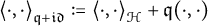 $$ \begin{align*}\left\langle {\cdot} , {\cdot} \right\rangle_{\mathfrak{q} +\mathfrak{id}} := \left\langle {\cdot} , {\cdot} \right\rangle_{\mathcal{H}} + \mathfrak{q} (\cdot , \cdot )\end{align*} $$
and $\mathfrak {q}$
is closeable if it has a closed extension. We will let
$\mathfrak {q}$
is closeable if it has a closed extension. We will let $\hat {\mathcal {H}} (\mathfrak {q})$
denote the Hilbert space completion of
$\hat {\mathcal {H}} (\mathfrak {q})$
denote the Hilbert space completion of $\mathrm {Dom} \, \mathfrak {q}$
with respect to this
$\mathrm {Dom} \, \mathfrak {q}$
with respect to this $\mathfrak {q}+\mathfrak {id}$
-inner product. Hence,
$\mathfrak {q}+\mathfrak {id}$
-inner product. Hence, $\mathfrak {q}$
is closed if and only if
$\mathfrak {q}$
is closed if and only if $\hat {\mathcal {H}} (\mathfrak {q}) = \mathrm {Dom} \, \mathfrak {q}$
. If
$\hat {\mathcal {H}} (\mathfrak {q}) = \mathrm {Dom} \, \mathfrak {q}$
. If $\mathfrak {q}\geq 0$
is closeable, then its closure,
$\mathfrak {q}\geq 0$
is closeable, then its closure, $\overline {\mathfrak {q}}$
, is the minimal closed extension of
$\overline {\mathfrak {q}}$
, is the minimal closed extension of $\mathfrak {q}$
. By Kato, closed positive semi-definite forms obey an “unbounded version” of the Riesz Lemma [Reference Kato16, Chapter VI, Theorems 2.1 and 2.23]. Namely,
$\mathfrak {q}$
. By Kato, closed positive semi-definite forms obey an “unbounded version” of the Riesz Lemma [Reference Kato16, Chapter VI, Theorems 2.1 and 2.23]. Namely, $\mathfrak {q} \geq 0$
is closed if and only if there is a unique self-adjoint, densely-defined and positive semi-definite operator, A, so that
$\mathfrak {q} \geq 0$
is closed if and only if there is a unique self-adjoint, densely-defined and positive semi-definite operator, A, so that $\mathrm {Dom} \, \mathfrak {q} = \mathrm {Dom} \, \sqrt {A}$
and
$\mathrm {Dom} \, \mathfrak {q} = \mathrm {Dom} \, \sqrt {A}$
and
 $$ \begin{align*}\mathfrak{q} (x,x) = \mathfrak{q}_A (x,x) = \left\langle {\sqrt{A} x} , {\sqrt{A} x} \right\rangle_{\mathcal{H}}.\end{align*} $$
Any self-adjoint operator is necessarily closed. Following Kato and Simon, we can define a partial order on densely-defined and positive semi-definite forms by $\mathfrak {q}_1 \leq \mathfrak {q}_2$
if:
$\mathfrak {q}_1 \leq \mathfrak {q}_2$
if:
-
(i)
$\mathrm {Dom} \, \mathfrak {q}_2 \subseteq \mathrm {Dom} \, \mathfrak {q}_1$
, and -
(ii)
$\mathfrak {q}_1 (x,x) \leq \mathfrak {q}_2 (x,x)$
for all
$x \in \mathrm {Dom} \, \mathfrak {q}_2$
.


In particular, if $\mathfrak {q}_A$
and
$\mathfrak {q}_A$
and $\mathfrak {q}_B$
are the closed forms of the self-adjoint and positive semi-definite operators A and B, we say that
$\mathfrak {q}_B$
are the closed forms of the self-adjoint and positive semi-definite operators A and B, we say that $A \leq B$
in the form sense if
$A \leq B$
in the form sense if $\mathfrak {q}_A \leq \mathfrak {q}_B$
as forms. This reduces to the usual Löwner partial order on bounded, self-adjoint operators, if A and B are bounded. At first sight, it may seem strange that the “larger” form in the above definition may have a smaller domain. The following result of Kato provides some justification for this (see [Reference Kato16, Chapter VI, Theorem 2.21], [Reference Simon22, Proposition 1.1]).
$\mathfrak {q}_A \leq \mathfrak {q}_B$
as forms. This reduces to the usual Löwner partial order on bounded, self-adjoint operators, if A and B are bounded. At first sight, it may seem strange that the “larger” form in the above definition may have a smaller domain. The following result of Kato provides some justification for this (see [Reference Kato16, Chapter VI, Theorem 2.21], [Reference Simon22, Proposition 1.1]).
Lemma 2.6 (Kato)
Let $A,B \geq 0$
be self-adjoint and densely-defined in
$A,B \geq 0$
be self-adjoint and densely-defined in $\mathcal {H}$
. Then
$\mathcal {H}$
. Then $A \leq B$
in the form sense if and only if
$A \leq B$
in the form sense if and only if
 $$ \begin{align*}( t I + A ) ^{-1} \leq (tI + B ) ^{-1},\end{align*} $$
for any $t>0$
.
$t>0$
.
Recall that if A is a closed operator with dense domain, $\mathrm {Dom} \, A \subseteq \mathcal {H}$
, that
$\mathrm {Dom} \, A \subseteq \mathcal {H}$
, that $\mathscr {D} \subseteq \mathrm {Dom} \, A$
is called a core for A, if A is equal to the closure of its restriction to
$\mathscr {D} \subseteq \mathrm {Dom} \, A$
is called a core for A, if A is equal to the closure of its restriction to $\mathscr {D}$
. Similarly, if
$\mathscr {D}$
. Similarly, if $\mathfrak {q}$
is a closed, densely-defined, and positive semi-definite form, a (necessarily dense) set
$\mathfrak {q}$
is a closed, densely-defined, and positive semi-definite form, a (necessarily dense) set $\mathscr {D} \subseteq \mathrm {Dom} \, \mathfrak {q}$
is called a form-core for
$\mathscr {D} \subseteq \mathrm {Dom} \, \mathfrak {q}$
is called a form-core for $\mathfrak {q}$
, if
$\mathfrak {q}$
, if $\mathscr {D}$
is dense in
$\mathscr {D}$
is dense in $\hat {\mathcal {H}} (\mathfrak {q})$
. It is not difficult to verify that if
$\hat {\mathcal {H}} (\mathfrak {q})$
. It is not difficult to verify that if $\mathfrak {q}=\mathfrak {q}_A$
is closed, then
$\mathfrak {q}=\mathfrak {q}_A$
is closed, then $\mathscr {D}$
is a form-core for
$\mathscr {D}$
is a form-core for $\mathfrak {q}$
if and only if
$\mathfrak {q}$
if and only if $\mathscr {D}$
is a core for
$\mathscr {D}$
is a core for $\sqrt {A}$
.
$\sqrt {A}$
.
Toeplitz forms. The classical Hardy space, $H^2 = H^2 (\mathbb {D} )$
, is the Hilbert space of square-summable Taylor series in the complex unit disk, equipped with the
$H^2 = H^2 (\mathbb {D} )$
, is the Hilbert space of square-summable Taylor series in the complex unit disk, equipped with the $\ell ^2$
-inner product of these coefficients. By results of Fatou, any element of
$\ell ^2$
-inner product of these coefficients. By results of Fatou, any element of $H^2$
has non-tangential boundary limits almost everywhere on the unit circle,
$H^2$
has non-tangential boundary limits almost everywhere on the unit circle, $\partial \mathbb {D}$
, with respect to normalized Lebesgue measure, m [Reference Hoffman13]. Identifying any
$\partial \mathbb {D}$
, with respect to normalized Lebesgue measure, m [Reference Hoffman13]. Identifying any $h \in H^2$
with its boundary limits defines an isometric inclusion of
$h \in H^2$
with its boundary limits defines an isometric inclusion of $H^2$
into
$H^2$
into $L^2 = L^2 (m)$
. Classically, Toeplitz operators, T, on
$L^2 = L^2 (m)$
. Classically, Toeplitz operators, T, on $H^2$
, are defined as the compression of bounded multiplication operators on
$H^2$
, are defined as the compression of bounded multiplication operators on $L^2$
to
$L^2$
to $H^2$
. Namely,
$H^2$
. Namely, $T = T_g := P_{H^2} M_g | _{H^2}$
, and
$T = T_g := P_{H^2} M_g | _{H^2}$
, and $\| T _g \| = \| M_g \| = \| g \| _\infty $
so that
$\| T _g \| = \| M_g \| = \| g \| _\infty $
so that $g \in L^\infty $
. A theorem of Brown and Halmos, [Reference Halmos and Brown10, Theorem 6], characterizes the Toeplitz operators as the set of all bounded operators, T, on
$g \in L^\infty $
. A theorem of Brown and Halmos, [Reference Halmos and Brown10, Theorem 6], characterizes the Toeplitz operators as the set of all bounded operators, T, on $H^2$
which obey the simple algebraic condition,
$H^2$
which obey the simple algebraic condition,
 $$ \begin{align*}S^* T S = T,\end{align*} $$
where $S = M_z$
, is the shift on
$S = M_z$
, is the shift on $H^2$
, the isometry of multiplication by z. Under the boundary value identification of
$H^2$
, the isometry of multiplication by z. Under the boundary value identification of $H^2$
with the subspace
$H^2$
with the subspace $H^2 (m) \subseteq L^2 (m , \partial \mathbb {D})$
, the shift is identified with the isometry
$H^2 (m) \subseteq L^2 (m , \partial \mathbb {D})$
, the shift is identified with the isometry $S=Z^m = M^m _\zeta |_{H^2(m)}$
.
$S=Z^m = M^m _\zeta |_{H^2(m)}$
.
Recall, as described in the Outline section, given a positive, finite, and regular Borel measure, $\mu $
, on
$\mu $
, on $\partial \mathbb {D}$
, we can associate with
$\partial \mathbb {D}$
, we can associate with $\mu $
the densely-defined and positive semi-definite quadratic form,
$\mu $
the densely-defined and positive semi-definite quadratic form, $\mathfrak {q} _\mu $
, with dense form domain,
$\mathfrak {q} _\mu $
, with dense form domain, $\mathrm {Dom} \, \mathfrak {q} _\mu := A (\mathbb {D} )$
in
$\mathrm {Dom} \, \mathfrak {q} _\mu := A (\mathbb {D} )$
in $H^2 = H^2 (m )$
, where m is normalized Lebesgue measure. This positive form,
$H^2 = H^2 (m )$
, where m is normalized Lebesgue measure. This positive form, $\mathfrak {q} _\mu $
, is an example of a Toeplitz form, as studied by Grenander and Szegö in [Reference Grenander and Szegö9]. Namely,
$\mathfrak {q} _\mu $
, is an example of a Toeplitz form, as studied by Grenander and Szegö in [Reference Grenander and Szegö9]. Namely, $\mathrm {Dom} \, \mathfrak {q}_\mu = A (\mathbb {D} )$
obeys
$\mathrm {Dom} \, \mathfrak {q}_\mu = A (\mathbb {D} )$
obeys $S \mathrm {Dom} \, \mathfrak {q}_\mu \subseteq \mathrm {Dom} \, \mathfrak {q}_\mu $
, and
$S \mathrm {Dom} \, \mathfrak {q}_\mu \subseteq \mathrm {Dom} \, \mathfrak {q}_\mu $
, and
 $$ \begin{align*}\mathfrak{q}_\mu (S x , Sy) = \mathfrak{q}_\mu (x,y); \quad \quad x,y \in A (\mathbb{D} ) = \mathrm{Dom} \, \mathfrak{q}_\mu.\end{align*} $$
If $\mathfrak {q}_\mu $
is closeable so that
$\mathfrak {q}_\mu $
is closeable so that $\overline {\mathfrak {q} _\mu } = \mathfrak {q}_T$
for a closed, self-adjoint
$\overline {\mathfrak {q} _\mu } = \mathfrak {q}_T$
for a closed, self-adjoint $T \geq 0$
, then by Kato’s unbounded Riesz lemma, we have that
$T \geq 0$
, then by Kato’s unbounded Riesz lemma, we have that $S^* T S = T$
, and our results will show that
$S^* T S = T$
, and our results will show that
 $$ \begin{align*}\mathfrak{q}_\mu (x,y) = \left\langle {M_{\sqrt{f}} x} , {M_{\sqrt{f}} y} \right\rangle_{L^2}; \quad \quad f = \frac{d\mu}{dm} \in L^1, \ x,y \in A (\mathbb{D} )\end{align*} $$
(see Theorem 4.12). Hence, $T = T_f = P_{H^2} M_f | _{H^2}$
is a closed, potentially unbounded Toeplitz operator with symbol f, in this “quadratic form sense.” In particular, if
$T = T_f = P_{H^2} M_f | _{H^2}$
is a closed, potentially unbounded Toeplitz operator with symbol f, in this “quadratic form sense.” In particular, if $T\geq 0$
is bounded, which happens if and only if
$T\geq 0$
is bounded, which happens if and only if $\mu \leq t^2 m$
for some
$\mu \leq t^2 m$
for some $t>0$
, then by the Riesz representation lemma,
$t>0$
, then by the Riesz representation lemma, $S^* T S = T$
, so that T is a bounded Toeplitz operator by Brown–Halmos, in which case
$S^* T S = T$
, so that T is a bounded Toeplitz operator by Brown–Halmos, in which case $T = T_f$
for
$T = T_f$
for $f = \frac {d\mu }{dm} \in L^\infty $
and
$f = \frac {d\mu }{dm} \in L^\infty $
and $\| f \| _\infty \leq t$
, by Theorem 4.1 and Corollary 4.2.
$\| f \| _\infty \leq t$
, by Theorem 4.1 and Corollary 4.2.
3 Spaces of Cauchy transforms
Let $\mu $
be a positive, finite, and regular Borel measure on the complex unit circle. Recall that given any
$\mu $
be a positive, finite, and regular Borel measure on the complex unit circle. Recall that given any $h \in H^2 (\mu ) = \mathbb {C} [ \zeta ] ^{- \| \cdot \| _{L^2 (\mu )}}$
, its
$h \in H^2 (\mu ) = \mathbb {C} [ \zeta ] ^{- \| \cdot \| _{L^2 (\mu )}}$
, its $\mu $
-Cauchy transform is the function
$\mu $
-Cauchy transform is the function
 $$ \begin{align} (\mathscr{C} _\mu h) (z) := \int _{\partial \mathbb{D} } h (\zeta) \, \frac{1}{1-z \overline{\zeta}} \mu (d\zeta) = \left\langle {k_z} , {h} \right\rangle_{L^2 (\mu )}; \quad k_z (\zeta ) := (1 - \overline{z} \zeta ) ^{-1}. \end{align} $$
We will call the functions $k_z$
,
$k_z$
, $z \in \mathbb {D}$
, Szegö kernel vectors.
$z \in \mathbb {D}$
, Szegö kernel vectors.
Recall that $A (\mathbb {D} )$
denotes the disk algebra, the unital Banach algebra of analytic functions in
$A (\mathbb {D} )$
denotes the disk algebra, the unital Banach algebra of analytic functions in $\mathbb {D}$
which extend continuously to the boundary,
$\mathbb {D}$
which extend continuously to the boundary, $\partial \mathbb {D}$
. Since the analytic polynomials are supremum-norm dense in
$\partial \mathbb {D}$
. Since the analytic polynomials are supremum-norm dense in $A (\mathbb {D} )$
, viewed as a subspace of the continuous functions,
$A (\mathbb {D} )$
, viewed as a subspace of the continuous functions, $\mathscr {C} (\partial \mathbb {D} )$
, on the circle and
$\mathscr {C} (\partial \mathbb {D} )$
, on the circle and $H^2 (\mu ) = A (\mathbb {D} ) ^{-\| \cdot \| _{L^2 (\mu )}}$
, it follows that
$H^2 (\mu ) = A (\mathbb {D} ) ^{-\| \cdot \| _{L^2 (\mu )}}$
, it follows that $H^2 (\mu ) = \mathbb {C} [\zeta ] ^{-\| \cdot \| _{L^2 (\mu )}} = A (\mathbb {D} ) ^{-\| \cdot \| _{L^2 (\mu )}}$
. Similarly,
$H^2 (\mu ) = \mathbb {C} [\zeta ] ^{-\| \cdot \| _{L^2 (\mu )}} = A (\mathbb {D} ) ^{-\| \cdot \| _{L^2 (\mu )}}$
. Similarly, $\mathscr {K} _{\mathbb {D}} := \bigvee _{z \in \mathbb {D}} k_z$
is also supremum-norm dense in
$\mathscr {K} _{\mathbb {D}} := \bigvee _{z \in \mathbb {D}} k_z$
is also supremum-norm dense in $A (\mathbb {D} ) \subseteq \mathscr {C} (\partial \mathbb {D} )$
, so that this subspace is also dense in
$A (\mathbb {D} ) \subseteq \mathscr {C} (\partial \mathbb {D} )$
, so that this subspace is also dense in $H^2 (\mu )$
.
$H^2 (\mu )$
.
Lemma 3.1 The $\mu $
-Cauchy transform of any
$\mu $
-Cauchy transform of any $h \in H^2 (\mu )$
is holomorphic in
$h \in H^2 (\mu )$
is holomorphic in $\mathbb {D}$
.
$\mathbb {D}$
.
Proof Given any $z \in \mathbb {D}$
, since
$z \in \mathbb {D}$
, since $(\mathscr {C} _\mu h) (z) := \left \langle {k_z} , {h} \right \rangle _{L^2 (\mu )}$
, consider the Leibniz difference quotient
$(\mathscr {C} _\mu h) (z) := \left \langle {k_z} , {h} \right \rangle _{L^2 (\mu )}$
, consider the Leibniz difference quotient
 $$ \begin{align*}\lim _{\epsilon \rightarrow 0} \frac{(\mathscr{C} _\mu h) (z +\epsilon ) -(\mathscr{C} _\mu h) (z)}{\epsilon } = \lim _{\epsilon \rightarrow 0} \epsilon ^{-1} \left\langle {k_{z+\epsilon } - k_z} , {h} \right\rangle_{L^2 (\mu )}.\end{align*} $$
(Here, recall that our inner products are conjugate linear in their first argument.) This limit will exist and $\mathscr {C} _\mu h$
will be holomorphic, if and only if the limit of
$\mathscr {C} _\mu h$
will be holomorphic, if and only if the limit of $\overline {\epsilon } ^{-1} (k_{z+\epsilon } - k_z)$
exists in
$\overline {\epsilon } ^{-1} (k_{z+\epsilon } - k_z)$
exists in $H^2 (\mu )$
. This limit exists in supremum norm on the circle (and so belongs to
$H^2 (\mu )$
. This limit exists in supremum norm on the circle (and so belongs to $A (\mathbb {D} )$
), and so it certainly exists in the
$A (\mathbb {D} )$
), and so it certainly exists in the $L^2 (\mu )$
-norm by Cauchy–Schwarz. Indeed,
$L^2 (\mu )$
-norm by Cauchy–Schwarz. Indeed,
 $$ \begin{align*} \lim _{\epsilon \rightarrow 0} \overline{\frac{k_{z+\epsilon } (\zeta ) - k_z (\zeta )}{\overline{\epsilon }}} & = \lim \frac{1 - \overline{\zeta} z - (1 - \overline{\zeta} z - \overline{\zeta} \epsilon )}{\epsilon (1 - \overline{\zeta} z) (1-\overline{\zeta} (z +\epsilon ))} \\ & = \frac{\overline{\zeta}}{(1-\overline{\zeta} z) ^2}, \end{align*} $$
and this limit is continuous on $\partial \mathbb {D}$
for any fixed
$\partial \mathbb {D}$
for any fixed $z \in \mathbb {D}$
. Hence
$z \in \mathbb {D}$
. Hence $\mathscr {C} _\mu h \in \mathscr {O} (\mathbb {D})$
for any
$\mathscr {C} _\mu h \in \mathscr {O} (\mathbb {D})$
for any $h \in H^2 (\mu )$
.
$h \in H^2 (\mu )$
.
Let $\mathscr {H} ^+ (\mu ) := \mathscr {C} _\mu H^2 (\mu ) \subseteq \mathscr {O} (\mathbb {D})$
be the complex vector space of
$\mathscr {H} ^+ (\mu ) := \mathscr {C} _\mu H^2 (\mu ) \subseteq \mathscr {O} (\mathbb {D})$
be the complex vector space of $\mu $
-Cauchy transforms equipped with the inner product,
$\mu $
-Cauchy transforms equipped with the inner product,
 $$ \begin{align*}\left\langle {\mathscr{C} _\mu g} , {\mathscr{C} _\mu h} \right\rangle_\mu := \left\langle {g} , {h} \right\rangle_{L^2 (\mu )}.\end{align*} $$
Lemma 3.2 The space of $\mu $
-Cauchy transforms,
$\mu $
-Cauchy transforms, $\mathscr {H} ^+ (\mu )$
, is a RKHS of analytic functions in
$\mathscr {H} ^+ (\mu )$
, is a RKHS of analytic functions in $\mathbb {D}$
with reproducing kernel
$\mathbb {D}$
with reproducing kernel
 $$ \begin{align*} k^\mu (z,w) & := \int _{\partial \mathbb{D}} \frac{1}{1-z \overline{\zeta}} \frac{1}{1-\overline{w} \zeta} \mu (d\zeta ) = \left\langle {k_z} , {k_w} \right\rangle_{L^2 (\mu )} \\ & = \frac{1}{2} \frac{H_\mu (z) + \overline{H_\mu (w)}}{1-z \overline{w}}, \end{align*} $$
where $H_\mu (z) = \int _{\partial \mathbb {D}} \frac {1 + z \overline {\zeta }}{1-z\overline {\zeta }} \mu (d\zeta )$
is the Herglotz–Riesz transform of
$H_\mu (z) = \int _{\partial \mathbb {D}} \frac {1 + z \overline {\zeta }}{1-z\overline {\zeta }} \mu (d\zeta )$
is the Herglotz–Riesz transform of $\mu $
.
$\mu $
.
By construction, $\mathscr {C} _\mu $
is an isometry of
$\mathscr {C} _\mu $
is an isometry of $H^2 (\mu )$
onto
$H^2 (\mu )$
onto $\mathscr {H} ^+ (\mu )$
.
$\mathscr {H} ^+ (\mu )$
.
Proof To show that this inner product is well-defined, we need to check that $\mathscr {C} _\mu h \equiv 0$
in the disk implies that
$\mathscr {C} _\mu h \equiv 0$
in the disk implies that $h=0$
in
$h=0$
in $H^2 (\mu )$
. Indeed,
$H^2 (\mu )$
. Indeed,
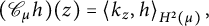 $$ \begin{align*}(\mathscr{C} _\mu h) (z) = \left\langle {k_z} , {h} \right\rangle_{H^2 (\mu )},\end{align*} $$
and since $\bigvee k_z$
is dense in
$\bigvee k_z$
is dense in $A (\mathbb {D})$
, the linear span of the Szegö kernels is also dense in
$A (\mathbb {D})$
, the linear span of the Szegö kernels is also dense in $H^2 (\mu )$
as described above. Hence, this vanishes for all
$H^2 (\mu )$
as described above. Hence, this vanishes for all $z \in \mathbb {D}$
if and only if
$z \in \mathbb {D}$
if and only if $h=0$
.
$h=0$
.
By definition, for any $z \in \mathbb {D}$
,
$z \in \mathbb {D}$
,
 $$ \begin{align*}(\mathscr{C} _\mu h) (z) = \left\langle {k_z} , {h} \right\rangle_{H^2 (\mu )} = \left\langle {\mathscr{C} _\mu k_z} , {\mathscr{C} _\mu h} \right\rangle_\mu,\end{align*} $$
so that $\mathscr {H} ^+ (\mu )$
is a RKHS in
$\mathscr {H} ^+ (\mu )$
is a RKHS in $\mathbb {D}$
with kernel vectors
$\mathbb {D}$
with kernel vectors $k ^\mu _z := \mathscr {C} _\mu k_z$
and reproducing kernel
$k ^\mu _z := \mathscr {C} _\mu k_z$
and reproducing kernel
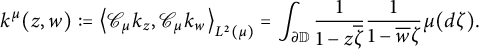 $$ \begin{align*}k^\mu (z,w) := \left\langle {\mathscr{C} _\mu k_z} , {\mathscr{C} _\mu k_w} \right\rangle_{L^2 (\mu )} = \int _{\partial \mathbb{D}} \frac{1}{1 -z \overline{\zeta}} \frac{1}{1-\overline{w} \zeta} \mu (d\zeta ).\end{align*} $$
Finally,
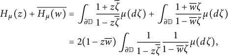 $$ \begin{align*} H_\mu (z) + \overline{H_\mu (w)} & = \int _{\partial \mathbb{D}} \frac{1 +z\overline{\zeta}}{1-z\overline{\zeta}} \mu (d\zeta ) + \int _{\partial \mathbb{D}} \frac{1 +\overline{w} \zeta}{1-\overline{w}\zeta} \mu (d\zeta ) \\ & = 2 (1 - z \overline{w} ) \int _{\partial \mathbb{D}} \frac{1}{1-z \overline{\zeta}} \frac{1}{1-\overline{w} \zeta} \mu (d\zeta ), \end{align*} $$
establishing the second formula.
Example 3.3 (Hardy space)
If $\mu =m$
is normalized Lebesgue measure, then
$\mu =m$
is normalized Lebesgue measure, then
 $$ \begin{align*} H_m (z) & := \int _{\partial \mathbb{D}} \frac{1 + z \overline{\zeta}}{1 -z \overline{\zeta}} m (d\zeta ) \\ & = \int _{\partial \mathbb{D}} \frac{2}{1 -z \overline{\zeta}} m (d\zeta ) - m (\partial \mathbb{D}) \\ & = \sum _{j=0} ^\infty z^j \int _{\partial \mathbb{D}} \overline{\zeta} ^j m (d\zeta ) - \int _{\partial \mathbb{D}} m (d\zeta ) \\ & = \sum _{j=0} ^\infty z^j \frac{1}{2\pi} \int _0 ^{2\pi} e^{-ij\theta} d\theta - \frac{1}{2\pi} \int _0 ^{2\pi} d\theta = 2 \delta _{j,0} - 1 =1. \end{align*} $$
It follows that $b_m := \frac {H_m -1}{H_m +1} \equiv 0$
, so that
$b_m := \frac {H_m -1}{H_m +1} \equiv 0$
, so that $m = \mu _0$
is the Clark measure of the identically
$m = \mu _0$
is the Clark measure of the identically $0$
function. Moreover,
$0$
function. Moreover,
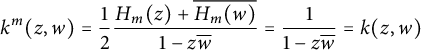 $$ \begin{align*}k^m (z,w) = \frac{1}{2} \frac{H_m (z) + \overline{H_m (w)}}{1-z\overline{w}} = \frac{1}{1-z\overline{w}} = k(z,w)\end{align*} $$
is the Szegö kernel. This is the reproducing kernel for the classical Hardy space $H^2 = H^2 (\mathbb {D} )$
, of square-summable Taylor series in the complex unit disk, equipped with the
$H^2 = H^2 (\mathbb {D} )$
, of square-summable Taylor series in the complex unit disk, equipped with the $\ell ^2$
-inner product of the Taylor coefficients. That is,
$\ell ^2$
-inner product of the Taylor coefficients. That is, $\mathscr {H} ^+ (m) = H^2$
.
$\mathscr {H} ^+ (m) = H^2$
.
Since any $h := \mathscr {C} _\mu g \in \mathscr {H} ^+ (\mu )$
is holomorphic in the open unit disk, its Taylor series at
$h := \mathscr {C} _\mu g \in \mathscr {H} ^+ (\mu )$
is holomorphic in the open unit disk, its Taylor series at $0$
has radius of convergence at least one,
$0$
has radius of convergence at least one,
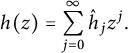 $$ \begin{align*}h(z) = \sum _{j=0} ^\infty \hat{h} _j z^j.\end{align*} $$
Moreover, expanding $k_z (\zeta )$
in a convergent geometric sum,
$k_z (\zeta )$
in a convergent geometric sum,
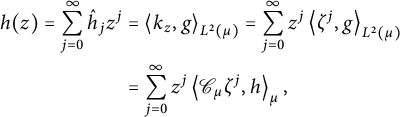 $$ \begin{align*} h(z) = \sum _{j=0} ^\infty \hat{h} _j z^j & = \left\langle {k_z} , {g} \right\rangle_{L^2 (\mu ) } = \sum _{j=0} ^\infty z^j \left\langle {\zeta ^j} , {g} \right\rangle_{L^2 (\mu )} \\ & = \sum _{j=0} ^\infty z^j \left\langle {\mathscr{C} _\mu \zeta ^j} , {h} \right\rangle_\mu, \end{align*} $$
and it follows that the Taylor coefficients are given by
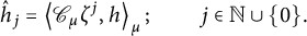 $$ \begin{align*}\hat{h} _j = \left\langle {\mathscr{C} _\mu \zeta ^j} , {h} \right\rangle_\mu; \quad \quad j \in \mathbb{N} \cup \{ 0 \}.\end{align*} $$
That is, for any $j \in \mathbb {N} \cup \{ 0 \}$
, the linear functionals
$j \in \mathbb {N} \cup \{ 0 \}$
, the linear functionals $\ell _j (h) = \hat {h} _j$
are bounded on
$\ell _j (h) = \hat {h} _j$
are bounded on $\mathscr {H} ^+ (\mu )$
and are implemented by inner products against the Taylor coefficient kernel vectors
$\mathscr {H} ^+ (\mu )$
and are implemented by inner products against the Taylor coefficient kernel vectors $k ^\mu _j := \mathscr {C} _\mu \zeta ^j$
. Hence,
$k ^\mu _j := \mathscr {C} _\mu \zeta ^j$
. Hence, $\mathscr {H} ^+ (\mu )$
is a Taylor coefficient RKHS in
$\mathscr {H} ^+ (\mu )$
is a Taylor coefficient RKHS in $\mathbb {D}$
with coefficient reproducing kernel,
$\mathbb {D}$
with coefficient reproducing kernel, $\hat {k} ^\mu (i,j)$
, on the set
$\hat {k} ^\mu (i,j)$
, on the set $\mathbb {N} \cup \{ 0 \}$
,
$\mathbb {N} \cup \{ 0 \}$
,
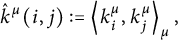 $$ \begin{align*}\hat{k} ^\mu (i,j) := \left\langle {k^\mu _i} , {k^\mu _j} \right\rangle_{\mu},\end{align*} $$
and $\hat {k} ^\mu $
is then a positive kernel function on
$\hat {k} ^\mu $
is then a positive kernel function on $\mathbb {N} \cup \{ 0 \}$
.
$\mathbb {N} \cup \{ 0 \}$
.
Given a positive measure $\mu $
, let
$\mu $
, let $V_\mu := \mathscr {C} _\mu Z^\mu \mathscr {C} _\mu ^*$
. This is an isometry on
$V_\mu := \mathscr {C} _\mu Z^\mu \mathscr {C} _\mu ^*$
. This is an isometry on $\mathscr {H} ^+ (\mu )$
that will play a central role in our analysis. This operator has a natural action on kernel vectors:
$\mathscr {H} ^+ (\mu )$
that will play a central role in our analysis. This operator has a natural action on kernel vectors:
 $$ \begin{align} V _\mu k^\mu _z \overline{z} = k^\mu _z - k^\mu _0, \quad \mbox{and} \quad V_\mu ^* (k^\mu _z - k^\mu _0) = k^\mu _z \overline{z}. \end{align} $$
In particular,
 $$ \begin{align*}\bigvee _{z \in \mathbb{D}} (k_z ^\mu - k_0 ^\mu ) = \mathrm{Ran} \, V_\mu,\end{align*} $$
where, here, $\bigvee $
denotes closed linear span. It is easy to check that a function,
$\bigvee $
denotes closed linear span. It is easy to check that a function, ${h \in \mathscr {H} ^+ (\mu )}$
, is orthogonal to
${h \in \mathscr {H} ^+ (\mu )}$
, is orthogonal to $\mathrm {Ran} \, V_\mu $
if and only if
$\mathrm {Ran} \, V_\mu $
if and only if $h = c 1$
,
$h = c 1$
, $c \in \mathbb {C}$
, is constant in the disk. Hence the following statements are equivalent:
$c \in \mathbb {C}$
, is constant in the disk. Hence the following statements are equivalent:
-
(i)
$\mu $
is extreme, -
(ii)
$H^2 (\mu ) = L^2 (\mu )$
, -
(iii)
$Z^\mu = M^\mu _\zeta | _{H^2 (\mu )}$
and hence
$V _\mu $
is unitary, -
(iv)
$\mathscr {H} ^+ (\mu )$
does not contain the constant functions.


Lemma 3.4 Given any finite, positive, and regular Borel measure, $\mu $
, on
$\mu $
, on $\partial \mathbb {D}$
, the co-isometry
$\partial \mathbb {D}$
, the co-isometry $V_\mu ^*$
, acts as a backward shift on
$V_\mu ^*$
, acts as a backward shift on $\mathscr {H} ^+ (\mu )$
, i.e., if
$\mathscr {H} ^+ (\mu )$
, i.e., if $h \in \mathscr {H} ^+ (\mu )$
,
$h \in \mathscr {H} ^+ (\mu )$
, $h(z) = \sum _{j=0} ^\infty \hat {h} _j z^j$
, then
$h(z) = \sum _{j=0} ^\infty \hat {h} _j z^j$
, then
 $$ \begin{align*}(V_\mu ^* h) (z) = \sum _{j=0} ^\infty \hat{h}_{j+1} z^j = \frac{h(z) - h(0)}{z}.\end{align*} $$
Given any $h \in \mathscr {H} ^+ (\mu )$
,
$h \in \mathscr {H} ^+ (\mu )$
,
 $$ \begin{align*}(V_\mu h) (z) = z h(z) + (V_\mu h) (0) 1.\end{align*} $$
Given any h in the classical Hardy space, $H^2 = \mathscr {H} ^+ (m)$
, one can check that
$H^2 = \mathscr {H} ^+ (m)$
, one can check that $S := V_m = M_z$
is the isometry of multiplication by the independent variable, z, on
$S := V_m = M_z$
is the isometry of multiplication by the independent variable, z, on $H^2$
, the shift. In this case, adjoint of S is called the backward shift and acts as
$H^2$
, the shift. In this case, adjoint of S is called the backward shift and acts as
 $$ \begin{align*}(S^*h) (z) = \frac{h(z) - h(0)}{z}.\end{align*} $$
It is straightforward to verify that if $h \in H^2$
has Taylor series
$h \in H^2$
has Taylor series $h(z) = \sum \hat {h} _j z^j$
, then
$h(z) = \sum \hat {h} _j z^j$
, then $(S^* h) (z) = \sum _{j=0} ^\infty \hat {h} _{j+1} z^j$
. This motivates the terminology “backward shift” in the above lemma statement. This lemma is easily verified and we omit the proof.
$(S^* h) (z) = \sum _{j=0} ^\infty \hat {h} _{j+1} z^j$
. This motivates the terminology “backward shift” in the above lemma statement. This lemma is easily verified and we omit the proof.
4 Absolute continuity in the reproducing kernel sense
Recall that given positive measures $\mu $
and
$\mu $
and $\lambda $
, we say that
$\lambda $
, we say that $\mu $
is dominated by
$\mu $
is dominated by $\lambda $
if there is a
$\lambda $
if there is a $t>0$
so that
$t>0$
so that $\mu \leq t^2 \lambda $
, and we say that
$\mu \leq t^2 \lambda $
, and we say that $\mu $
is reproducing kernel or RK-dominated by
$\mu $
is reproducing kernel or RK-dominated by $\lambda $
, if
$\lambda $
, if $\mathscr {H} ^+ (\mu ) \subseteq \mathscr {H} ^+ (\lambda )$
and there is a
$\mathscr {H} ^+ (\mu ) \subseteq \mathscr {H} ^+ (\lambda )$
and there is a $t>0$
so that the norm of the embedding
$t>0$
so that the norm of the embedding $\mathrm {e} _{\mu , \lambda } : \mathscr {H} ^+ (\mu ) \hookrightarrow \mathscr {H} ^+ (\lambda )$
is at most t, written
$\mathrm {e} _{\mu , \lambda } : \mathscr {H} ^+ (\mu ) \hookrightarrow \mathscr {H} ^+ (\lambda )$
is at most t, written $\mu \leq _{RK} t^2 \lambda $
. We will begin this section by showing that these two definitions of domination are equivalent.
$\mu \leq _{RK} t^2 \lambda $
. We will begin this section by showing that these two definitions of domination are equivalent.
Theorem 4.1 Given positive, finite, and regular Borel measures $\mu , \lambda $
on the unit circle,
$\mu , \lambda $
on the unit circle, $\mu \leq t^2 \lambda $
for some
$\mu \leq t^2 \lambda $
for some $t>0$
if and only if
$t>0$
if and only if $\mu \leq _{RK} t^2 \lambda $
.
$\mu \leq _{RK} t^2 \lambda $
.
Proof (Necessity) If $\mu \leq t^2 \lambda $
, then
$\mu \leq t^2 \lambda $
, then $\gamma := t^2 \lambda - \mu $
is a positive measure and
$\gamma := t^2 \lambda - \mu $
is a positive measure and
 $$ \begin{align*} t^2 k^\lambda (z,w) - k^\mu (z,w) & = t^2 \int _{\partial \mathbb{D}} \frac{1}{1-z\overline{\zeta}}\frac{1}{1-\overline{w}\zeta} \lambda (d\zeta ) - \int _{\partial \mathbb{D}} \frac{1}{1-z\overline{\zeta}}\frac{1}{1-\overline{w}\zeta} \mu (d\zeta ) \\ & = \int _{\partial \mathbb{D}} \frac{1}{1-z\overline{\zeta}}\frac{1}{1-\overline{w}\zeta} \gamma (d\zeta ) = k^\gamma (z,w). \end{align*} $$
It follows that $t^2 k^\lambda - k^\mu = k^\gamma $
is a positive kernel so that
$t^2 k^\lambda - k^\mu = k^\gamma $
is a positive kernel so that $k^\mu \leq t^2 k^\lambda $
.
$k^\mu \leq t^2 k^\lambda $
.
First proof of sufficiency. Conversely, suppose that $K:= t^2 k ^\lambda - k^\mu \geq 0$
is a positive kernel. View the analytic polynomials,
$K:= t^2 k ^\lambda - k^\mu \geq 0$
is a positive kernel. View the analytic polynomials, $\mathbb {C} [ \zeta ]$
, as a dense subspace of the disk algebra
$\mathbb {C} [ \zeta ]$
, as a dense subspace of the disk algebra $A (\mathbb {D} )$
, embedded isometrically in the Banach space
$A (\mathbb {D} )$
, embedded isometrically in the Banach space $\mathscr {C} (\partial \mathbb {D} )$
. For any finite, positive and regular Borel measure on the complex unit circle,
$\mathscr {C} (\partial \mathbb {D} )$
. For any finite, positive and regular Borel measure on the complex unit circle, $\mu $
, we define the positive linear functional,
$\mu $
, we define the positive linear functional, $\hat {\mu }$
on
$\hat {\mu }$
on $\mathscr {C} (\partial \mathbb {D})$
by
$\mathscr {C} (\partial \mathbb {D})$
by
 $$ \begin{align*}\hat{\mu} (f) := \int _{\partial \mathbb{D}} f d\mu.\end{align*} $$
(The map $\mu \mapsto \hat {\mu }$
is a bijection, by the Riesz–Markov theorem.) We then define a bounded linear functional,
$\mu \mapsto \hat {\mu }$
is a bijection, by the Riesz–Markov theorem.) We then define a bounded linear functional, $\ell _K$
on
$\ell _K$
on $\mathscr {C} (\partial \mathbb {D})$
by
$\mathscr {C} (\partial \mathbb {D})$
by $\ell _K := t^2 \hat {\lambda } - \hat {\mu }$
.
$\ell _K := t^2 \hat {\lambda } - \hat {\mu }$
.
By Weierstraß approximation, $\mathbb {C} [ \zeta ] + \overline {\mathbb {C} [ \zeta ] }$
is supremum-norm dense in the continuous functions,
$\mathbb {C} [ \zeta ] + \overline {\mathbb {C} [ \zeta ] }$
is supremum-norm dense in the continuous functions, $\mathscr {C} (\partial \mathbb {D} )$
. Since the Fejér kernel is positive semi-definite, the partial Cesàro sums of any positive semi-definite
$\mathscr {C} (\partial \mathbb {D} )$
. Since the Fejér kernel is positive semi-definite, the partial Cesàro sums of any positive semi-definite $f \in \mathscr {C} (\partial \mathbb {D} )$
will be a positive trigonometric polynomial, i.e., a positive semi-definite element of
$f \in \mathscr {C} (\partial \mathbb {D} )$
will be a positive trigonometric polynomial, i.e., a positive semi-definite element of $\mathbb {C} [\zeta ] + \overline {\mathbb {C} [\zeta ]}$
and, by Fourier theory, it follows that the positive cone of
$\mathbb {C} [\zeta ] + \overline {\mathbb {C} [\zeta ]}$
and, by Fourier theory, it follows that the positive cone of $\mathbb {C} [ \zeta ] + \overline {\mathbb {C} [ \zeta ] }$
is supremum norm-dense in the positive cone of
$\mathbb {C} [ \zeta ] + \overline {\mathbb {C} [ \zeta ] }$
is supremum norm-dense in the positive cone of $\mathscr {C} (\partial \mathbb {D})$
. Moreover, by the Fejér–Riesz theorem, any positive trigonometric polynomial,
$\mathscr {C} (\partial \mathbb {D})$
. Moreover, by the Fejér–Riesz theorem, any positive trigonometric polynomial, $p + \overline {q} \geq 0$
, on
$p + \overline {q} \geq 0$
, on $\partial \mathbb {D}$
factors as
$\partial \mathbb {D}$
factors as $|g| ^2$
for an analytic
$|g| ^2$
for an analytic $g \in \mathbb {C} [\zeta ]$
(and necessarily,
$g \in \mathbb {C} [\zeta ]$
(and necessarily, $p =q$
,
$p =q$
, $\mathrm {deg} (p) = \mathrm {deg} (g)$
). Hence, to check that
$\mathrm {deg} (p) = \mathrm {deg} (g)$
). Hence, to check that $\ell _K$
is a positive linear functional on
$\ell _K$
is a positive linear functional on $\mathscr {C} (\partial \mathbb {D} )$
, it suffices to check that
$\mathscr {C} (\partial \mathbb {D} )$
, it suffices to check that $\ell _K ( p + \overline {p} ) \geq 0$
for any
$\ell _K ( p + \overline {p} ) \geq 0$
for any $p + \overline {p} = |g| ^2 \geq 0$
,
$p + \overline {p} = |g| ^2 \geq 0$
, $p, g \in \mathbb {C} [ \zeta ]$
. If
$p, g \in \mathbb {C} [ \zeta ]$
. If $p = \sum _{j=0} ^n \hat {p} _j \zeta ^j$
and
$p = \sum _{j=0} ^n \hat {p} _j \zeta ^j$
and $g = \sum _{j=0} ^n \hat {g} _j \zeta ^j$
, then by construction
$g = \sum _{j=0} ^n \hat {g} _j \zeta ^j$
, then by construction
 $$ \begin{align*}\left\langle {\mathscr{C} _\mu g} , {\mathscr{C} _\mu g} \right\rangle_\mu = \left\langle {g} , {g} \right\rangle_{H^2 (\mu) } = \left\langle {p} , {1} \right\rangle_{H^2 (\mu)} + \left\langle {1} , {p} \right\rangle_{H^2 (\mu )} = \left\langle {\mathscr{C} _\mu p} , {\mathscr{C} _\mu 1} \right\rangle_\mu + \left\langle {\mathscr{C} _\mu 1} , {\mathscr{C} _\mu p} \right\rangle_{\mu}.\end{align*} $$
Since
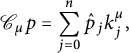 $$ \begin{align*}\mathscr{C} _\mu p = \sum _{j=0} ^n \hat{p} _j k ^\mu _j,\end{align*} $$
where the $k^\mu _j$
,
$k^\mu _j$
, $j \in \mathbb {N} \cup \{ 0 \}$
are the Taylor coefficient evaluation vectors, and since similar formulas hold for
$j \in \mathbb {N} \cup \{ 0 \}$
are the Taylor coefficient evaluation vectors, and since similar formulas hold for $\lambda $
, we obtain that
$\lambda $
, we obtain that
 $$ \begin{align*}\ell _K (|g| ^2) = \int _{\partial \mathbb{D}} |g (\zeta ) | ^2 (t^2 \lambda (d\zeta ) - \mu (d\zeta ) ) = \sum _{i,j=0} ^n \overline{\hat{g} _i} \hat{g} _j \left\langle {K_i} , {K_j} \right\rangle_{\mathcal{H} (K)},\end{align*} $$
where the $K_i$
,
$K_i$
, $i \in \mathbb {N} \cup \{ 0 \}$
are the Taylor coefficient evaluation vectors in
$i \in \mathbb {N} \cup \{ 0 \}$
are the Taylor coefficient evaluation vectors in $\mathcal {H} (K)$
. Namely,
$\mathcal {H} (K)$
. Namely, $\mathcal {H} (K)$
is also a Taylor coefficient RKHS in
$\mathcal {H} (K)$
is also a Taylor coefficient RKHS in $\mathbb {D}$
so that
$\mathbb {D}$
so that $\hat {K} (i , j) := \left \langle {K_i} , {K_j} \right \rangle _{\mathcal {H} (K)}$
defines a positive kernel function on the set
$\hat {K} (i , j) := \left \langle {K_i} , {K_j} \right \rangle _{\mathcal {H} (K)}$
defines a positive kernel function on the set $\mathbb {N} \cup \{ 0 \}$
. It follows that
$\mathbb {N} \cup \{ 0 \}$
. It follows that
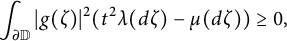 $$ \begin{align*}\int _{\partial \mathbb{D}} |g (\zeta ) | ^2 (t^2 \lambda (d\zeta ) - \mu (d\zeta ) ) \geq 0,\end{align*} $$
for any $g \in \mathbb {C} [ \zeta ]$
, or, equivalently,
$g \in \mathbb {C} [ \zeta ]$
, or, equivalently,
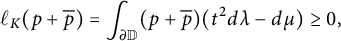 $$ \begin{align*}\ell _K (p + \overline{p}) = \int _{\partial \mathbb{D}} (p + \overline{p} ) (t^2 d\lambda - d\mu ) \geq 0,\end{align*} $$
for any positive semi-definite $p + \overline {p} \in \mathbb {C} [\zeta ] + \overline {\mathbb {C} [ \zeta ]}$
. By density of the positive cone of
$p + \overline {p} \in \mathbb {C} [\zeta ] + \overline {\mathbb {C} [ \zeta ]}$
. By density of the positive cone of $\mathbb {C} [\zeta ] + \overline {\mathbb {C} [\zeta ] }$
in the positive cone of the continuous functions, it follows that
$\mathbb {C} [\zeta ] + \overline {\mathbb {C} [\zeta ] }$
in the positive cone of the continuous functions, it follows that $\ell _K$
is a bounded, positive linear functional on
$\ell _K$
is a bounded, positive linear functional on $\mathscr {C} (\partial \mathbb {D} )$
, with norm
$\mathscr {C} (\partial \mathbb {D} )$
, with norm $\| \ell _K \| = \ell _K (1) = t^2 \lambda (\partial \mathbb {D} ) - \mu (\partial \mathbb {D} ) = K( 0, 0) \geq 0$
. By the Riesz–Markov theorem, there is then a unique, positive, finite, and regular Borel measure,
$\| \ell _K \| = \ell _K (1) = t^2 \lambda (\partial \mathbb {D} ) - \mu (\partial \mathbb {D} ) = K( 0, 0) \geq 0$
. By the Riesz–Markov theorem, there is then a unique, positive, finite, and regular Borel measure, $\gamma $
, on
$\gamma $
, on $\partial \mathbb {D}$
, so that
$\partial \mathbb {D}$
, so that
 $$ \begin{align*}\ell _K (f) = \int _{\partial \mathbb{D}} f(\zeta ) \gamma (d\zeta ),\end{align*} $$
for any $f \in \mathscr {C} (\partial \mathbb {D} )$
, i.e.,
$f \in \mathscr {C} (\partial \mathbb {D} )$
, i.e., $\ell _K = \hat {\gamma }$
, and we conclude that
$\ell _K = \hat {\gamma }$
, and we conclude that $\gamma = t^2 \lambda - \mu \geq 0$
so that
$\gamma = t^2 \lambda - \mu \geq 0$
so that $t^2 \lambda \geq \mu $
.
$t^2 \lambda \geq \mu $
.
Second proof of sufficiency. If $t^2 k^\lambda \geq k^\mu $
, then by Aronszajn’s inclusion theorem,
$t^2 k^\lambda \geq k^\mu $
, then by Aronszajn’s inclusion theorem, $\mathscr {H} ^+ (\mu ) \subseteq \mathscr {H} ^+ (\lambda )$
and the norm of the embedding
$\mathscr {H} ^+ (\mu ) \subseteq \mathscr {H} ^+ (\lambda )$
and the norm of the embedding $\mathrm {e} _{\mu , \lambda } : \mathscr {H} ^+ (\mu ) \hookrightarrow \mathscr {H} ^+ (\lambda )$
is at most
$\mathrm {e} _{\mu , \lambda } : \mathscr {H} ^+ (\mu ) \hookrightarrow \mathscr {H} ^+ (\lambda )$
is at most $t>0$
. Observe that
$t>0$
. Observe that $\mathrm {e} := \mathrm {e} _{\mu , \lambda }$
acts trivially as a multiplier by the constant function
$\mathrm {e} := \mathrm {e} _{\mu , \lambda }$
acts trivially as a multiplier by the constant function $1$
, so that
$1$
, so that
 $$ \begin{align*}\mathrm{e} ^* k ^\lambda _z = k^\mu _z, \quad \mbox{and} \quad \mathrm{e} ^* k^\lambda _j = k^\mu _j,\end{align*} $$
for any $z \in \mathbb {D}$
and
$z \in \mathbb {D}$
and $j \in \mathbb {N} \cup \{ 0 \}$
. Hence,
$j \in \mathbb {N} \cup \{ 0 \}$
. Hence,
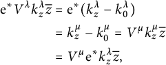 $$ \begin{align*} \mathrm{e} ^* V^\lambda k^\lambda _z \overline{z} & = \mathrm{e} ^* ( k^\lambda _z - k ^\lambda _0 ) \\ & = k^\mu _z - k ^\mu _0 = V^\mu k^\mu _z \overline{z} \\ & = V^\mu \mathrm{e} ^* k^\lambda _z \overline{z}, \end{align*} $$
so that $\mathrm {e} ^*$
intertwines
$\mathrm {e} ^*$
intertwines $V^\lambda $
with
$V^\lambda $
with $V^\mu $
,
$V^\mu $
, $\mathrm {e} ^* V^\lambda = V^\mu \mathrm {e} ^*$
. Setting
$\mathrm {e} ^* V^\lambda = V^\mu \mathrm {e} ^*$
. Setting $E := \mathscr {C} _\mu ^* \mathrm {e} ^* \mathscr {C} _\lambda $
, we see that for any monomial,
$E := \mathscr {C} _\mu ^* \mathrm {e} ^* \mathscr {C} _\lambda $
, we see that for any monomial,
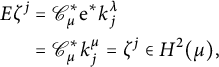 $$ \begin{align*} E \zeta ^j & = \mathscr{C} _\mu ^* \mathrm{e} ^* k^\lambda _j \\ & = \mathscr{C} _\mu ^* k^\mu _j = \zeta ^j \in H^2 (\mu ), \end{align*} $$
so that $E : H^2 (\lambda ) \hookrightarrow H^2 (\mu )$
obeys
$E : H^2 (\lambda ) \hookrightarrow H^2 (\mu )$
obeys $Ep =p$
for any
$Ep =p$
for any $p \in \mathbb {C} [\zeta ] \subseteq H^2 (\lambda )$
. In particular,
$p \in \mathbb {C} [\zeta ] \subseteq H^2 (\lambda )$
. In particular, $E Z^\lambda = Z^\mu E$
. At this point one could argue using the Riesz–Markov theorem as above, however, here is an alternative argument. Since
$E Z^\lambda = Z^\mu E$
. At this point one could argue using the Riesz–Markov theorem as above, however, here is an alternative argument. Since $Z^\lambda $
and
$Z^\lambda $
and $Z^\mu $
are contractions (they are isometries), we can apply the intertwining version of the commutant lifting theorem [Reference Paulsen19, Corollary 5.9] to conclude that E can be “lifted” to a bounded operator
$Z^\mu $
are contractions (they are isometries), we can apply the intertwining version of the commutant lifting theorem [Reference Paulsen19, Corollary 5.9] to conclude that E can be “lifted” to a bounded operator $\hat {E} : L^2 (\lambda ) \rightarrow L^2 (\mu )$
, with norm
$\hat {E} : L^2 (\lambda ) \rightarrow L^2 (\mu )$
, with norm $\| \hat {E} \| = \| E \|$
, so that
$\| \hat {E} \| = \| E \|$
, so that $\hat {E} M^\lambda _\zeta = M^\mu _\zeta \hat {E}$
, and
$\hat {E} M^\lambda _\zeta = M^\mu _\zeta \hat {E}$
, and $P _{H^2 (\mu )} \hat {E} | _{H ^2 (\lambda )} = E$
. Setting
$P _{H^2 (\mu )} \hat {E} | _{H ^2 (\lambda )} = E$
. Setting $\hat {T} := \hat {E}^* \hat {E} \in \mathscr {L} (L ^2 (\lambda ) )$
,
$\hat {T} := \hat {E}^* \hat {E} \in \mathscr {L} (L ^2 (\lambda ) )$
, $\hat {T} \geq 0$
is a positive semi-definite
$\hat {T} \geq 0$
is a positive semi-definite $M^\lambda _\zeta $
-Toeplitz operator in the sense that
$M^\lambda _\zeta $
-Toeplitz operator in the sense that
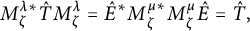 $$ \begin{align*}M^{\lambda *} _\zeta \hat{T} M^\lambda _\zeta = \hat{E} ^* M^{\mu *} _\zeta M^\mu _\zeta \hat{E} = \hat{T},\end{align*} $$
since $M ^\lambda _\zeta , M^\mu _\zeta $
are isometries. Since,
$M ^\lambda _\zeta , M^\mu _\zeta $
are isometries. Since, $M^\lambda _\zeta $
(and
$M^\lambda _\zeta $
(and $M^\mu _\zeta $
) is in fact unitary, it follows that
$M^\mu _\zeta $
) is in fact unitary, it follows that $\hat {T}$
commutes with
$\hat {T}$
commutes with $M^\lambda _\zeta $
. Since
$M^\lambda _\zeta $
. Since $\mathbb {C} [\zeta ] + \overline {\mathbb {C} [\zeta ]} \subseteq \mathrm {Ran} \, M^\lambda _\zeta $
is a dense set in
$\mathbb {C} [\zeta ] + \overline {\mathbb {C} [\zeta ]} \subseteq \mathrm {Ran} \, M^\lambda _\zeta $
is a dense set in $L^2 (\lambda )$
, a simple argument shows that
$L^2 (\lambda )$
, a simple argument shows that $\hat {T}$
acts as multiplication by
$\hat {T}$
acts as multiplication by $f:=T1 \in L^2 (\lambda )$
. However, since
$f:=T1 \in L^2 (\lambda )$
. However, since ${T = M_f}$
is a bounded and positive semi-definite operator, it is easy to check that
${T = M_f}$
is a bounded and positive semi-definite operator, it is easy to check that $t ^2 \geq \| \hat {T} \| = \| f \| _{\infty }$
,
$t ^2 \geq \| \hat {T} \| = \| f \| _{\infty }$
, $\| \hat {T} \| = \| \hat {E} \| ^2 = \| E \| ^2 = \| T \|$
, and
$\| \hat {T} \| = \| \hat {E} \| ^2 = \| E \| ^2 = \| T \|$
, and $f \geq 0\ \lambda $
-a.e. Finally, one can also check that
$f \geq 0\ \lambda $
-a.e. Finally, one can also check that $T = P_{H^2 (\lambda )} \hat {T} | _{H^2 (\lambda )}$
is
$T = P_{H^2 (\lambda )} \hat {T} | _{H^2 (\lambda )}$
is $Z^\lambda $
-Toeplitz, i.e.,
$Z^\lambda $
-Toeplitz, i.e., $Z^{\lambda *} T Z^\lambda =T$
. In conclusion, for any
$Z^{\lambda *} T Z^\lambda =T$
. In conclusion, for any $p, q \in \mathbb {C} [\zeta ]$
,
$p, q \in \mathbb {C} [\zeta ]$
,
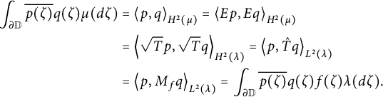 $$ \begin{align*} \int _{\partial \mathbb{D}} \overline{p (\zeta)} q (\zeta ) \mu (d\zeta ) & = \left\langle {p} , {q} \right\rangle_{H^2 (\mu )} = \left\langle {Ep} , {Eq} \right\rangle_{H^2 (\mu )} \\ & = \left\langle {\sqrt{T} p} , {\sqrt{T}q} \right\rangle_{H^2 (\lambda )} = \left\langle {p} , {\hat{T} q} \right\rangle_{L^2 (\lambda )} \\ & = \left\langle {p} , {M_f q} \right\rangle_{L ^2 (\lambda )} = \int _{\partial \mathbb{D}} \overline{p (\zeta )} q (\zeta) f(\zeta ) \lambda (d\zeta ). \end{align*} $$
This formula extends to elements of the form $g= \overline {p} + q \in \mathbb {C} [\zeta ] + \overline {\mathbb {C} [\zeta ]}$
since
$g= \overline {p} + q \in \mathbb {C} [\zeta ] + \overline {\mathbb {C} [\zeta ]}$
since
 $$ \begin{align*}\left\langle {\overline{p} _1 + q_1} , {\overline{p_2} + q_2} \right\rangle_{L^2 (\mu )} = \left\langle {q_1} , {q_2} \right\rangle_{H^2 (\mu )} + \left\langle {q_1 p_2} , {1} \right\rangle_{H^2 (\mu)} + \left\langle {p_2} , {p_1} \right\rangle_{H^2 (\mu )} + \left\langle {1} , {p_1 q_2} \right\rangle_{H^2 (\mu )}\!.\end{align*} $$
Again, by Weierstraß approximation, since $\mathbb {C} [\zeta ] + \overline {\mathbb {C} [\zeta ]}$
is supremum-norm dense in
$\mathbb {C} [\zeta ] + \overline {\mathbb {C} [\zeta ]}$
is supremum-norm dense in $\mathscr {C} (\partial \mathbb {D} )$
, which is in turn dense in
$\mathscr {C} (\partial \mathbb {D} )$
, which is in turn dense in $L^2 (\lambda )$
and
$L^2 (\lambda )$
and $L^2 (\mu )$
, it follows that for any
$L^2 (\mu )$
, it follows that for any $g, h \in L^2 (\lambda )$
,
$g, h \in L^2 (\lambda )$
,
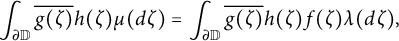 $$ \begin{align*}\int _{\partial \mathbb{D}} \overline{g (\zeta )} h (\zeta ) \mu (d\zeta ) = \int _{\partial \mathbb{D}} \overline{g (\zeta )} h (\zeta ) f(\zeta ) \lambda (d\zeta ),\end{align*} $$
where $f \geq 0$
,
$f \geq 0$
, $\lambda $
-a.e. and
$\lambda $
-a.e. and $\| f \| _\infty \leq t^2$
. We conclude that
$\| f \| _\infty \leq t^2$
. We conclude that $\mu \leq t^2 \lambda $
and that
$\mu \leq t^2 \lambda $
and that
 $$ \begin{align*}f = \frac{\mu (d\zeta )}{\lambda (d\zeta )},\end{align*} $$
is the (bounded) Radon–Nikodym derivative of $\mu $
with respect to
$\mu $
with respect to $\lambda $
.
$\lambda $
.
Definition 1 Let $T \in \mathscr {L} (\mathcal {H} )$
be a bounded operator, and let V be an isometry on
$T \in \mathscr {L} (\mathcal {H} )$
be a bounded operator, and let V be an isometry on $\mathcal {H}$
. We say that T is V-Toeplitz if
$\mathcal {H}$
. We say that T is V-Toeplitz if
 $$ \begin{align*}V^* T V = T.\end{align*} $$
If $\mathfrak {q} \geq 0$
is a positive semi-definite quadratic form with dense form domain,
$\mathfrak {q} \geq 0$
is a positive semi-definite quadratic form with dense form domain, $\mathrm {Dom} \, \mathfrak {q} \subseteq \mathcal {H}$
, we say that
$\mathrm {Dom} \, \mathfrak {q} \subseteq \mathcal {H}$
, we say that $\mathfrak {q}$
is V-Toeplitz if
$\mathfrak {q}$
is V-Toeplitz if $\mathrm {Dom} \, \mathfrak {q}$
is V-invariant and
$\mathrm {Dom} \, \mathfrak {q}$
is V-invariant and
 $$ \begin{align*}\mathfrak{q} (Vg , Vh) = \mathfrak{q} (g,h); \quad \quad g,h \in \mathrm{Dom} \, \mathfrak{q}.\end{align*} $$
In particular, if $T\geq 0$
is a positive semi-definite, self-adjoint and densely-defined operator in
$T\geq 0$
is a positive semi-definite, self-adjoint and densely-defined operator in $\mathcal {H}$
, we say that T is V-Toeplitz if the closed, positive semi-definite form it generates,
$\mathcal {H}$
, we say that T is V-Toeplitz if the closed, positive semi-definite form it generates,
 $$ \begin{align*}\mathfrak{q} _T (x,y) := \left\langle {\sqrt{T} x} , {\sqrt{T} y} \right\rangle_{\mathcal{H}}; \quad \quad x,y \in \mathrm{Dom} \, \mathfrak{q} _T = \mathrm{Dom} \, \sqrt{T},\end{align*} $$
is V-Toeplitz. If $T\geq 0$
is bounded, this latter definition reduces to the definition of a bounded, positive semi-definite V-Toeplitz operator.
$T\geq 0$
is bounded, this latter definition reduces to the definition of a bounded, positive semi-definite V-Toeplitz operator.
Corollary 4.2 Let $\mu , \lambda $
be positive, finite, and regular Borel measures on
$\mu , \lambda $
be positive, finite, and regular Borel measures on $\partial \mathbb {D}$
so that
$\partial \mathbb {D}$
so that $\mu \leq t^2 \lambda $
. In this case,
$\mu \leq t^2 \lambda $
. In this case,
 $$ \begin{align*}E_{\mu , \lambda } := \mathscr{C} _\mu ^* \mathrm{e} _{\mu , \lambda } ^* \mathscr{C} _\lambda : H^2 (\lambda ) \hookrightarrow H^2 (\mu), \end{align*} $$
is a co-embedding in the sense that $E _{\mu ,\lambda } p = p$
for any
$E _{\mu ,\lambda } p = p$
for any $p \in \mathbb {C} [\zeta ]$
. Moreover,
$p \in \mathbb {C} [\zeta ]$
. Moreover,
 $$ \begin{align*}\mathrm{e} _{\mu , \lambda } ^* k ^\lambda _z = k^\mu _z, \quad \mathrm{e} _{\mu , \lambda } ^* k^\lambda _j = k^\mu _j, \quad \quad \forall \ z \in \mathbb{D}, \ j \in \mathbb{N} \cup \{ 0 \},\end{align*} $$ $\mathrm {e} _{\mu ,\lambda } ^* V_\lambda = V^\mu \mathrm {e} _{\mu , \lambda } ^*$
and equivalently
$\mathrm {e} _{\mu ,\lambda } ^* V_\lambda = V^\mu \mathrm {e} _{\mu , \lambda } ^*$
and equivalently $E_{\mu , \lambda } Z ^\lambda = Z^\mu E_{\mu , \lambda }$
. If
$E_{\mu , \lambda } Z ^\lambda = Z^\mu E_{\mu , \lambda }$
. If $T_\mu := E _{\mu , \lambda } ^* E _{\mu ,\lambda }$
, then
$T_\mu := E _{\mu , \lambda } ^* E _{\mu ,\lambda }$
, then $T_\mu $
is
$T_\mu $
is $Z^\lambda $
-Toeplitz and T is the compression of a bounded multiplication operator,
$Z^\lambda $
-Toeplitz and T is the compression of a bounded multiplication operator, $T = P_{H^2 (\lambda )} M_f |_{H^2 (\lambda )}$
, where
$T = P_{H^2 (\lambda )} M_f |_{H^2 (\lambda )}$
, where $f \geq 0\ \lambda -a.e.$
,
$f \geq 0\ \lambda -a.e.$
, $\| f \| _{\infty } \leq t^2$
, and
$\| f \| _{\infty } \leq t^2$
, and $f = \frac {\mu (d\zeta ) }{\lambda (d\zeta )}$
is the Radon–Nikodym derivative of
$f = \frac {\mu (d\zeta ) }{\lambda (d\zeta )}$
is the Radon–Nikodym derivative of $\mu $
with respect to
$\mu $
with respect to $\lambda $
.
$\lambda $
.
Remark 4.3 While the co-embedding, $E_{\mu , \lambda } : H^2 (\lambda ) \hookrightarrow H^2 (\mu )$
always has dense range, it may have nontrivial kernel. For example, if
$E_{\mu , \lambda } : H^2 (\lambda ) \hookrightarrow H^2 (\mu )$
always has dense range, it may have nontrivial kernel. For example, if $\lambda $
is the sum of two Dirac point masses at distinct points
$\lambda $
is the sum of two Dirac point masses at distinct points $\zeta , \xi \in \partial \mathbb {D}$
,
$\zeta , \xi \in \partial \mathbb {D}$
, $\mu $
is the point mass at
$\mu $
is the point mass at $\zeta $
, then
$\zeta $
, then $\mu \leq \lambda $
and if p is any polynomial vanishing at
$\mu \leq \lambda $
and if p is any polynomial vanishing at $\zeta $
, then
$\zeta $
, then $E_{\mu , \lambda } p =0 \in H^2 (\mu )$
. To be precise,
$E_{\mu , \lambda } p =0 \in H^2 (\mu )$
. To be precise, $H^2 (\mu )$
is the closure of the disk algebra,
$H^2 (\mu )$
is the closure of the disk algebra, $A (\mathbb {D} )$
, or the polynomials,
$A (\mathbb {D} )$
, or the polynomials, $\mathbb {C} [\zeta ]$
, in the
$\mathbb {C} [\zeta ]$
, in the $L^2 (\mu )$
-norm, so that if
$L^2 (\mu )$
-norm, so that if $p \in \mathbb {C} [\zeta ]$
or
$p \in \mathbb {C} [\zeta ]$
or $a \in A (\mathbb {D} )$
vanishes on the support of
$a \in A (\mathbb {D} )$
vanishes on the support of $\mu $
, then
$\mu $
, then $p=0=a$
in
$p=0=a$
in $H^2 (\mu )$
.
$H^2 (\mu )$
.
More generally, absolute continuity of positive measures can also be described in terms of their spaces of Cauchy transforms. It is a straightforward exercise, using the Radon–Nikodym formula, to show that $\mu $
is absolutely continuous with respect to
$\mu $
is absolutely continuous with respect to $\lambda $
, if and only if one can construct a monotonically increasing sequence of positive measures,
$\lambda $
, if and only if one can construct a monotonically increasing sequence of positive measures, $\mu _n \geq 0$
, so that
$\mu _n \geq 0$
, so that $\mu _n \leq \mu $
for all n, the
$\mu _n \leq \mu $
for all n, the $\mu _n \uparrow \mu $
increase monotonically to
$\mu _n \uparrow \mu $
increase monotonically to $\mu $
, and there is a sequence of positive constants,
$\mu $
, and there is a sequence of positive constants, $t_n>0$
so that
$t_n>0$
so that $\mu _n \leq t_n ^2 \lambda $
. Indeed, this can be readily established by taking the “join” or point-wise maxima of
$\mu _n \leq t_n ^2 \lambda $
. Indeed, this can be readily established by taking the “join” or point-wise maxima of $\frac {d\mu }{d\lambda }$
and the constant functions
$\frac {d\mu }{d\lambda }$
and the constant functions $t_n ^2 \cdot 1$
. Since
$t_n ^2 \cdot 1$
. Since $\mu _n \leq \mu $
for all n, Aronszajn’s inclusion theorem implies that
$\mu _n \leq \mu $
for all n, Aronszajn’s inclusion theorem implies that $\mathscr {H} ^+ (\mu _n ) \subseteq \mathscr {H} ^+ (\mu )$
and that the embeddings
$\mathscr {H} ^+ (\mu _n ) \subseteq \mathscr {H} ^+ (\mu )$
and that the embeddings $\mathrm {e} _n : \mathscr {H} ^+ (\mu _n ) \hookrightarrow \mathscr {H} ^+ (\mu )$
are all contractive. Moreover, and again by Aronszajn’s inclusion theorem, each
$\mathrm {e} _n : \mathscr {H} ^+ (\mu _n ) \hookrightarrow \mathscr {H} ^+ (\mu )$
are all contractive. Moreover, and again by Aronszajn’s inclusion theorem, each $\mathscr {H} ^+ (\mu _n ) \subseteq \mathscr {H} ^+ (\lambda )$
is boundedly contained in
$\mathscr {H} ^+ (\mu _n ) \subseteq \mathscr {H} ^+ (\lambda )$
is boundedly contained in $\mathscr {H} ^+ (\lambda )$
so that
$\mathscr {H} ^+ (\lambda )$
so that
 $$ \begin{align} \mathscr{H} ^+ (\mu _n ) \subseteq \mathscr{H} ^+ (\mu ) \cap \mathscr{H} ^+ (\lambda )=:\mathrm{int} (\mu , \lambda ). \end{align} $$
Proposition 4.4 If $\mu \ll \lambda $
, then the intersection space,
$\mu \ll \lambda $
, then the intersection space, $\mathrm {int} (\mu , \lambda ) = \mathscr {H} ^+ (\mu ) \cap \mathscr {H} ^+ (\lambda )$
is dense in
$\mathrm {int} (\mu , \lambda ) = \mathscr {H} ^+ (\mu ) \cap \mathscr {H} ^+ (\lambda )$
is dense in $\mathscr {H} ^+ (\mu )$
.
$\mathscr {H} ^+ (\mu )$
.
Proof We have that for all n, $0 \leq \mu _n \leq \mu $
and
$0 \leq \mu _n \leq \mu $
and $\mu _n \uparrow \mu $
. Moreover,
$\mu _n \uparrow \mu $
. Moreover, $\mathscr {H} ^+ (\mu _n ) \subseteq \mathrm {int} (\mu , \lambda )$
for all n. If
$\mathscr {H} ^+ (\mu _n ) \subseteq \mathrm {int} (\mu , \lambda )$
for all n. If $1 \geq g_n \geq 0, \mu -a.e.$
are the Radon–Nikodym derivatives of the
$1 \geq g_n \geq 0, \mu -a.e.$
are the Radon–Nikodym derivatives of the $\mu _n$
with respect to
$\mu _n$
with respect to $\mu $
, and
$\mu $
, and $p \in \mathbb {C} [\zeta ]$
, let
$p \in \mathbb {C} [\zeta ]$
, let $\mathscr {C} _n := \mathscr {C} _{\mu _n}$
and let
$\mathscr {C} _n := \mathscr {C} _{\mu _n}$
and let $\mathrm {e} _n : \mathscr {H} ^+ (\mu _n ) \hookrightarrow \mathscr {H} ^+ (\mu )$
. Then,
$\mathrm {e} _n : \mathscr {H} ^+ (\mu _n ) \hookrightarrow \mathscr {H} ^+ (\mu )$
. Then,
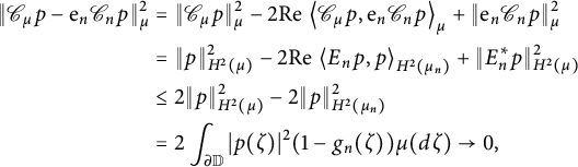 $$ \begin{align*} \| \mathscr{C} _\mu p - \mathrm{e} _n \mathscr{C} _n p \| ^2 _\mu & = \| \mathscr{C} _\mu p \| ^2 _\mu -2 \mathrm{Re} \, \left\langle {\mathscr{C} _\mu p} , {\mathrm{e} _n \mathscr{C} _n p} \right\rangle_\mu + \| \mathrm{e} _n \mathscr{C} _n p \| ^2 _\mu \\ & = \| p \| ^2 _{H^2 (\mu)} - 2 \mathrm{Re} \, \left\langle {E_n p} , {p} \right\rangle_{H^2 (\mu _n )} + \| E_n ^* p \| ^2 _{H^2 (\mu)} \\ & \leq 2 \| p \| ^2 _{H^2 (\mu )} - 2 \| p \| ^2 _{H^2 (\mu _n )} \\ & = 2 \int _{\partial \mathbb{D}} | p (\zeta ) | ^2 (1 - g_n (\zeta ) ) \mu (d\zeta ) \rightarrow 0, \end{align*} $$
by the Lebesgue monotone convergence theorem. In conclusion,
 $$ \begin{align*}\mathscr{H} ^+ (\mu ) = \bigvee _{n=1} ^\infty \mathscr{H} ^+ (\mu _n ),\end{align*} $$
where, here, $\bigvee $
denotes closed linear span.
$\bigvee $
denotes closed linear span.
This motivates the following definitions:
Definition 2 Let $\mu , \lambda $
be finite, positive, and regular Borel measures on
$\mu , \lambda $
be finite, positive, and regular Borel measures on $\partial \mathbb {D}$
. We say that
$\partial \mathbb {D}$
. We say that $\mu $
is absolutely continuous with respect to
$\mu $
is absolutely continuous with respect to $\lambda $
in the reproducing kernel sense,
$\lambda $
in the reproducing kernel sense, $\mu \ll _{RK} \lambda $
, if the intersection space,
$\mu \ll _{RK} \lambda $
, if the intersection space,
 $$ \begin{align*}\mathrm{int} (\mu , \lambda ) = \mathscr{H} ^+ (\mu ) \cap \mathscr{H} ^+ (\lambda )\end{align*} $$
is norm-dense in $\mathscr {H} ^+ (\mu )$
.
$\mathscr {H} ^+ (\mu )$
.
We say that $\mu $
is reproducing kernel singular with respect to
$\mu $
is reproducing kernel singular with respect to $\lambda $
, written
$\lambda $
, written $\mu \perp _{RK} \lambda $
, if the intersection space is trivial,
$\mu \perp _{RK} \lambda $
, if the intersection space is trivial, $\mathrm {int} (\mu , \lambda ) = \{ 0 \}$
.
$\mathrm {int} (\mu , \lambda ) = \{ 0 \}$
.
By the previous proposition, $\mu \ll \lambda $
implies that
$\mu \ll \lambda $
implies that $\mu \ll _{RK} \lambda $
. The main result of this section will be to show that this new “reproducing kernel” definition of absolute continuity is equivalent to the classical one.
$\mu \ll _{RK} \lambda $
. The main result of this section will be to show that this new “reproducing kernel” definition of absolute continuity is equivalent to the classical one.
Lemma 4.5 If $\mu \ll _{RK} \lambda $
, then the embedding,
$\mu \ll _{RK} \lambda $
, then the embedding, $\mathrm {e} _{\mu , \lambda } : \mathrm {int} (\mu ,\lambda ) \subseteq \mathscr {H} ^+ (\mu ) \hookrightarrow \mathscr {H} ^+ (\lambda )$
, is closed with dense domain
$\mathrm {e} _{\mu , \lambda } : \mathrm {int} (\mu ,\lambda ) \subseteq \mathscr {H} ^+ (\mu ) \hookrightarrow \mathscr {H} ^+ (\lambda )$
, is closed with dense domain $\mathrm {int} (\mu , \lambda )$
. In this case, the co-embedding,
$\mathrm {int} (\mu , \lambda )$
. In this case, the co-embedding, $E _{\mu ,\lambda } : \mathrm {Dom} \, E _{\mu ,\lambda } \subseteq H^2 (\lambda ) \hookrightarrow H^2 (\mu )$
, is densely-defined and closed. Both
$E _{\mu ,\lambda } : \mathrm {Dom} \, E _{\mu ,\lambda } \subseteq H^2 (\lambda ) \hookrightarrow H^2 (\mu )$
, is densely-defined and closed. Both $\mathbb {C} [ \zeta ]$
and
$\mathbb {C} [ \zeta ]$
and $\mathscr {K} _{\mathbb {D}} = \bigvee _{z \in \mathbb {D} } k_z$
are cores for
$\mathscr {K} _{\mathbb {D}} = \bigvee _{z \in \mathbb {D} } k_z$
are cores for $E_{\mu ,\lambda }$
and
$E_{\mu ,\lambda }$
and $E_{\mu ,\lambda } k_z = k_z$
,
$E_{\mu ,\lambda } k_z = k_z$
, $E_{\mu , \lambda } p = p$
for all
$E_{\mu , \lambda } p = p$
for all $k_z \in \mathscr {K} _{\mathbb {D}}$
and
$k_z \in \mathscr {K} _{\mathbb {D}}$
and $p \in \mathbb {C} [\zeta ]$
. The (closed) self-adjoint and positive semi-definite operator,
$p \in \mathbb {C} [\zeta ]$
. The (closed) self-adjoint and positive semi-definite operator, $T_\mu := E_{\mu ,\lambda } ^* E_{\mu , \lambda }$
is
$T_\mu := E_{\mu ,\lambda } ^* E_{\mu , \lambda }$
is $Z^\lambda $
-Toeplitz.
$Z^\lambda $
-Toeplitz.
Proof Let $\mathrm {e} := \mathrm {e} _{\mu ,\lambda }$
and observe that
$\mathrm {e} := \mathrm {e} _{\mu ,\lambda }$
and observe that $\mathrm {e}$
is, trivially, a multiplier by the constant function
$\mathrm {e}$
is, trivially, a multiplier by the constant function $1$
from
$1$
from $\mathscr {H} ^+ (\mu )$
into
$\mathscr {H} ^+ (\mu )$
into $\mathscr {H} ^+ (\lambda )$
. By Proposition 2.1 and Remark 2.2,
$\mathscr {H} ^+ (\lambda )$
. By Proposition 2.1 and Remark 2.2, $\mathrm {e}$
is closed on its maximal domain,
$\mathrm {e}$
is closed on its maximal domain, $\mathrm {int} (\mu , \lambda )$
, its adjoint acts as
$\mathrm {int} (\mu , \lambda )$
, its adjoint acts as
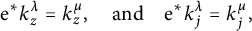 $$ \begin{align*}\mathrm{e} ^* k^\lambda _z = k^\mu _z, \quad \mbox{and} \quad \mathrm{e} ^* k^\lambda _j = k^\mu _j,\end{align*} $$
on kernels and coefficient kernels and the linear spans of the point evaluation and Taylor coefficient kernels in $\mathscr {H} ^+ (\lambda )$
are both cores for
$\mathscr {H} ^+ (\lambda )$
are both cores for $\mathrm {e} ^*$
. Since
$\mathrm {e} ^*$
. Since $E = E_{\mu , \lambda } := \mathscr {C} _\mu ^* \mathrm {e} ^* \mathscr {C} _\lambda $
, E is closed, the formulas
$E = E_{\mu , \lambda } := \mathscr {C} _\mu ^* \mathrm {e} ^* \mathscr {C} _\lambda $
, E is closed, the formulas $E p = p$
for
$E p = p$
for $p \in \mathbb {C} [\zeta ]$
and
$p \in \mathbb {C} [\zeta ]$
and $E k_z = k_z$
are easily verified, and it further follows that
$E k_z = k_z$
are easily verified, and it further follows that $\mathscr {K} _{\mathbb {D}}$
and
$\mathscr {K} _{\mathbb {D}}$
and $\mathbb {C} [\zeta ]$
are cores for E.
$\mathbb {C} [\zeta ]$
are cores for E.
To check that $T:= T_\mu = E_{\mu ,\lambda } ^* E_{\mu ,\lambda } \geq 0$
is
$T:= T_\mu = E_{\mu ,\lambda } ^* E_{\mu ,\lambda } \geq 0$
is $\lambda $
-Toeplitz, consider, for any
$\lambda $
-Toeplitz, consider, for any $p, q \in \mathbb {C} [\zeta ]$
,
$p, q \in \mathbb {C} [\zeta ]$
,
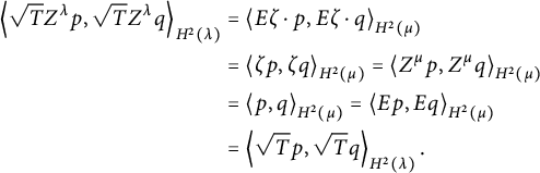 $$ \begin{align*} \left\langle {\sqrt{T} Z^\lambda p} , {\sqrt{T} Z^\lambda q} \right\rangle_{H^2 (\lambda )} & = \left\langle { E \zeta \cdot p} , {E \zeta \cdot q} \right\rangle_{H^2 (\mu )} \\ & = \left\langle { \zeta p} , {\zeta q} \right\rangle_{H^2 (\mu )} = \left\langle {Z^\mu p} , {Z^\mu q} \right\rangle_{H^2 (\mu )} \\ & = \left\langle {p} , {q} \right\rangle_{H^2 (\mu )} = \left\langle {Ep} , {Eq} \right\rangle_{H^2 (\mu )} \\ & = \left\langle {\sqrt{T} p} , {\sqrt{T} q} \right\rangle_{H^2 (\lambda )}. \end{align*} $$
As the polynomials are a core for $E = E_{\mu ,\lambda }$
, this calculation holds on
$E = E_{\mu ,\lambda }$
, this calculation holds on $\mathrm {Dom} \, E = \mathrm {Dom} \, \sqrt {T}$
. Moreover, since
$\mathrm {Dom} \, E = \mathrm {Dom} \, \sqrt {T}$
. Moreover, since $\mathrm {Dom} \, E = \mathrm {Dom} \, \sqrt {T}$
, by polar decomposition of closed operators, and since
$\mathrm {Dom} \, E = \mathrm {Dom} \, \sqrt {T}$
, by polar decomposition of closed operators, and since $\mathbb {C} [\zeta ]$
and
$\mathbb {C} [\zeta ]$
and $\mathscr {K} _{\mathbb {D}}$
are
$\mathscr {K} _{\mathbb {D}}$
are $Z^\lambda $
-invariant cores for E, they are also cores for
$Z^\lambda $
-invariant cores for E, they are also cores for $\sqrt {T}$
, and it follows that
$\sqrt {T}$
, and it follows that $\mathrm {Dom} \, \sqrt {T} _\mu = \mathrm {Dom} \, E$
is also
$\mathrm {Dom} \, \sqrt {T} _\mu = \mathrm {Dom} \, E$
is also $Z^\lambda $
-invariant.
$Z^\lambda $
-invariant.
Proposition 4.6 Given $\mu , \lambda \geq 0$
, if
$\mu , \lambda \geq 0$
, if $\lambda $
is extreme, then
$\lambda $
is extreme, then $\mu \ll _{RK} \lambda $
if and only if
$\mu \ll _{RK} \lambda $
if and only if $\mu \ll \lambda $
.
$\mu \ll \lambda $
.
Proof Recall that $\lambda $
is extreme if and only if
$\lambda $
is extreme if and only if $H^2 (\lambda ) = L^2 (\lambda )$
so that
$H^2 (\lambda ) = L^2 (\lambda )$
so that $Z^\lambda = M^\lambda _{\zeta }$
. In this case, the self-adjoint
$Z^\lambda = M^\lambda _{\zeta }$
. In this case, the self-adjoint $\lambda $
-Toeplitz operator
$\lambda $
-Toeplitz operator $T_\mu \geq 0$
is Toeplitz with respect to the unitary
$T_\mu \geq 0$
is Toeplitz with respect to the unitary $M^\lambda _\zeta $
. That is,
$M^\lambda _\zeta $
. That is,
 $$ \begin{align*}\left\langle {\sqrt{T_\mu} M^\lambda _\zeta h} , {\sqrt{T_\mu} M^\lambda _\zeta h} \right\rangle_{H^2 (\lambda )} = \left\langle {\sqrt{T_\mu} h} , {\sqrt{T_\mu} h} \right\rangle_{H^2 (\lambda )},\end{align*} $$
for all $h \in \mathrm {Dom} \, \sqrt {T_\mu }$
. Hence the quadratic forms for
$h \in \mathrm {Dom} \, \sqrt {T_\mu }$
. Hence the quadratic forms for $(M^\lambda _\zeta ) ^* T _\mu M^\lambda _\zeta $
and
$(M^\lambda _\zeta ) ^* T _\mu M^\lambda _\zeta $
and $T_\mu $
are the same. By uniqueness of the unbounded Riesz representation,
$T_\mu $
are the same. By uniqueness of the unbounded Riesz representation, $(M^\lambda _\zeta ) ^* T_\mu M^\lambda _\zeta = T_\mu $
, so that, by Lemma 2.6,
$(M^\lambda _\zeta ) ^* T_\mu M^\lambda _\zeta = T_\mu $
, so that, by Lemma 2.6,
 $$ \begin{align*}( I + (M^\lambda _\zeta) ^* T_\mu M^\lambda _\zeta ) ^{-1} = ( I + T _\mu ) ^{-1},\end{align*} $$
or, equivalently,
 $$ \begin{align*}M^\lambda _\zeta (I + T_\mu ) ^{-1} = (I + T_\mu ) ^{-1} M^\lambda _\zeta.\end{align*} $$
This shows that $T_\mu $
, and hence
$T_\mu $
, and hence $\sqrt {T} _\mu $
are affiliated to the commutant of the unitary operator
$\sqrt {T} _\mu $
are affiliated to the commutant of the unitary operator $M^\lambda _\zeta $
. Since
$M^\lambda _\zeta $
. Since $\mathbb {C} [\zeta ] \subseteq \mathrm {Dom} \, \sqrt {T_\mu }$
, we conclude that
$\mathbb {C} [\zeta ] \subseteq \mathrm {Dom} \, \sqrt {T_\mu }$
, we conclude that $\sqrt {T _\mu } = M _{\sqrt {T_\mu } 1}$
acts as multiplication by
$\sqrt {T _\mu } = M _{\sqrt {T_\mu } 1}$
acts as multiplication by $\sqrt {T _\mu } 1 =: f \in L^2 (\lambda )$
. Since
$\sqrt {T _\mu } 1 =: f \in L^2 (\lambda )$
. Since $\sqrt {T _\mu } \geq 0$
, we necessarily have that
$\sqrt {T _\mu } \geq 0$
, we necessarily have that $f\geq 0$
,
$f\geq 0$
, $\lambda -a.e.$
, and we conclude that for any polynomials
$\lambda -a.e.$
, and we conclude that for any polynomials $p,q$
,
$p,q$
,
 $$ \begin{align*}\left\langle {p} , {q} \right\rangle_{H^2 (\mu )} = \left\langle {\sqrt{T_\mu}p} , {\sqrt{T_\mu }q} \right\rangle_{H^2 (\lambda )} = \int _{\partial \mathbb{D}} \overline{p (\zeta )} q(\zeta ) f (\zeta ) ^2 \lambda (d\zeta ).\end{align*} $$
As in the proof of sufficiency in Theorem 4.1, we conclude that the above formula holds for any $g,h \in \mathbb {C} [\zeta ] + \overline {\mathbb {C} [\zeta ]}$
, which is dense in
$g,h \in \mathbb {C} [\zeta ] + \overline {\mathbb {C} [\zeta ]}$
, which is dense in $\mathscr {C} (\partial \mathbb {D} )$
and
$\mathscr {C} (\partial \mathbb {D} )$
and $L^\infty (\mu )$
. In particular, the formula holds for all simple functions and characteristic functions of Borel sets. Since
$L^\infty (\mu )$
. In particular, the formula holds for all simple functions and characteristic functions of Borel sets. Since $f \in L^2 (\lambda )$
,
$f \in L^2 (\lambda )$
, $f^2 \in L^1 (\lambda )$
and it follows that
$f^2 \in L^1 (\lambda )$
and it follows that
 $$ \begin{align*}f^2 = \frac{\mu (d\zeta )}{\lambda (d\zeta )}\end{align*} $$
is the Radon–Nikodym derivative of $\mu $
with respect to
$\mu $
with respect to $\lambda $
.
$\lambda $
.
To prove that absolute continuity in the reproducing kernel sense is equivalent to absolute continuity in general, we will appeal to B. Simon’s Lebesgue decomposition theory for positive quadratic forms in Hilbert space (see [Reference Reed and Simon21, Supplement to VIII.7], [Reference Simon22]). Let $\hat {\mathcal {H}} (\mathfrak {q})$
be the Hilbert space completion of
$\hat {\mathcal {H}} (\mathfrak {q})$
be the Hilbert space completion of $\mathrm {Dom} \, \mathfrak {q}$
with respect to the inner product
$\mathrm {Dom} \, \mathfrak {q}$
with respect to the inner product $\left \langle {\cdot } , {\cdot } \right \rangle _{\mathcal {H}} + \mathfrak {q} (\cdot , \cdot )$
, and let
$\left \langle {\cdot } , {\cdot } \right \rangle _{\mathcal {H}} + \mathfrak {q} (\cdot , \cdot )$
, and let $\mathrm {j} _{\mathfrak {q}} : \mathrm {Dom} \, \mathfrak {q} \hookrightarrow \hat {\mathcal {H}} (\mathfrak {q} )$
denote the formal embedding. Further, define the co-embedding
$\mathrm {j} _{\mathfrak {q}} : \mathrm {Dom} \, \mathfrak {q} \hookrightarrow \hat {\mathcal {H}} (\mathfrak {q} )$
denote the formal embedding. Further, define the co-embedding $E_{\mathfrak {q}} : \hat {\mathcal {H}} (\mathfrak {q} )\hookrightarrow \mathcal {H}$
by
$E_{\mathfrak {q}} : \hat {\mathcal {H}} (\mathfrak {q} )\hookrightarrow \mathcal {H}$
by
 $$ \begin{align*}E _{\mathfrak{q}} (\mathrm{j} _{\mathfrak{q}} (x) ) := x, \quad \quad x \in \mathrm{Dom} \, \mathfrak{q}.\end{align*} $$
By construction, $\mathrm {j} _{\mathfrak {q}}$
is densely-defined, has dense range, and
$\mathrm {j} _{\mathfrak {q}}$
is densely-defined, has dense range, and $E_{\mathfrak {q}}$
is contractive with dense range in
$E_{\mathfrak {q}}$
is contractive with dense range in $\mathcal {H}$
. Hence,
$\mathcal {H}$
. Hence, $E_{\mathfrak {q}}$
extends by continuity to a contraction, also denoted by
$E_{\mathfrak {q}}$
extends by continuity to a contraction, also denoted by $E_{\mathfrak {q}}$
,
$E_{\mathfrak {q}}$
, $E_{\mathfrak {q}} : \hat {\mathcal {H}} (\mathfrak {q} ) \hookrightarrow \mathcal {H}$
.
$E_{\mathfrak {q}} : \hat {\mathcal {H}} (\mathfrak {q} ) \hookrightarrow \mathcal {H}$
.
Lemma 4.7 A densely-defined and positive semi-definite quadratic form, $\mathfrak {q}$
, in
$\mathfrak {q}$
, in $\mathcal {H}$
, is closeable if and only if
$\mathcal {H}$
, is closeable if and only if $\mathrm {j} _{\mathfrak {q}}$
is closeable, or equivalently, if and only if
$\mathrm {j} _{\mathfrak {q}}$
is closeable, or equivalently, if and only if $E_{\mathfrak {q}}$
is injective.
$E_{\mathfrak {q}}$
is injective.
This lemma is a straightforward consequence of the definitions (see also [Reference Simon22]).
Theorem 4.8 (Simon–Lebesgue decomposition of positive forms)
Let $\mathfrak {q} \geq 0$
be a positive semi-definite quadratic form with dense form domain,
$\mathfrak {q} \geq 0$
be a positive semi-definite quadratic form with dense form domain, $\mathrm {Dom} \, \mathfrak {q}$
, in a separable, complex Hilbert space,
$\mathrm {Dom} \, \mathfrak {q}$
, in a separable, complex Hilbert space, $\mathcal {H}$
. Then
$\mathcal {H}$
. Then $\mathfrak {q}$
has a unique Lebesgue decomposition,
$\mathfrak {q}$
has a unique Lebesgue decomposition, ${\mathfrak {q} = \mathfrak {q}_{ac} + \mathfrak {q} _s}$
, where
${\mathfrak {q} = \mathfrak {q}_{ac} + \mathfrak {q} _s}$
, where $0 \leq \mathfrak {q}_{ac}, \mathfrak {q} _s \leq \mathfrak {q}$
in the quadratic form sense,
$0 \leq \mathfrak {q}_{ac}, \mathfrak {q} _s \leq \mathfrak {q}$
in the quadratic form sense, $\mathfrak {q} _{ac}$
is the maximal absolutely continuous form less than or equal to
$\mathfrak {q} _{ac}$
is the maximal absolutely continuous form less than or equal to $\mathfrak {q}$
and
$\mathfrak {q}$
and $\mathfrak {q} _s$
is a singular form.
$\mathfrak {q} _s$
is a singular form.
If $P_s$
denotes the projection onto
$P_s$
denotes the projection onto $\mathrm {Ker} \, E_{\mathfrak {q}}$
, and
$\mathrm {Ker} \, E_{\mathfrak {q}}$
, and $P_{ac} = I - P_s$
, then
$P_{ac} = I - P_s$
, then $\mathfrak {q}_{ac}$
is given by the formula,
$\mathfrak {q}_{ac}$
is given by the formula,
 $$ \begin{align} \mathfrak{q}_{ac} (x,y) = \left\langle { \mathrm{j} _{\mathfrak{q}} (x) } , {(P_{ac} - E _{\mathfrak{q}} ^* E_{\mathfrak{q}} ) \mathrm{j} _{\mathfrak{q}} (y)} \right\rangle_{\hat{\mathcal{H}} (\mathfrak{q})} = \left\langle { \mathrm{j} _{\mathfrak{q}} (x) } , {P_{ac} \, \mathrm{j} _{\mathfrak{q}} (y)} \right\rangle_{\hat{\mathcal{H}} (\mathfrak{q})} - \left\langle {x} , {y} \right\rangle_{\mathcal{H}}. \end{align} $$
In the above theorem statement, recall that we defined the notions of an absolutely continuous or singular positive quadratic form in the introduction. Namely, a positive semi-definite and densely-defined quadratic form, $\mathfrak {q} : \mathrm {Dom} \, \mathfrak {q} \times \mathrm {Dom} \, \mathfrak {q} \rightarrow \mathcal {H}$
,
$\mathfrak {q} : \mathrm {Dom} \, \mathfrak {q} \times \mathrm {Dom} \, \mathfrak {q} \rightarrow \mathcal {H}$
, $\mathrm {Dom} \, \mathfrak {q} \subseteq \mathcal {H}$
, is called absolutely continuous if it is closeable, and singular if the only absolutely continuous and positive semi-definite form it dominates is the identically zero form.
$\mathrm {Dom} \, \mathfrak {q} \subseteq \mathcal {H}$
, is called absolutely continuous if it is closeable, and singular if the only absolutely continuous and positive semi-definite form it dominates is the identically zero form.
Remark 4.9 If, now, $\mu , \lambda \geq 0$
are measures on the circle, we can take
$\mu , \lambda \geq 0$
are measures on the circle, we can take $\mathcal {H} := L^2 (\lambda )$
or
$\mathcal {H} := L^2 (\lambda )$
or $H^2 (\lambda )$
, and define
$H^2 (\lambda )$
, and define $\mathfrak {q} _\mu \geq 0$
on a dense form domain in
$\mathfrak {q} _\mu \geq 0$
on a dense form domain in $\mathcal {H}$
by the formula
$\mathcal {H}$
by the formula
 $$ \begin{align*}\mathfrak{q}_\mu (f,g) = \int _{\partial \mathbb{D}} \overline{f(\zeta)} g(\zeta ) \mu (d\zeta ).\end{align*} $$
For example, if $\mathcal {H} = L^2 (\lambda )$
, one can take
$\mathcal {H} = L^2 (\lambda )$
, one can take $\mathrm {Dom} \, \mathfrak {q}_\mu = \mathscr {C} (\partial \mathbb {D} )$
, the continuous functions. In this case, by the remark on [Reference Simon22, p. 381], the quadratic form Lebesgue decomposition of
$\mathrm {Dom} \, \mathfrak {q}_\mu = \mathscr {C} (\partial \mathbb {D} )$
, the continuous functions. In this case, by the remark on [Reference Simon22, p. 381], the quadratic form Lebesgue decomposition of $\mathfrak {q}_\mu $
coincides with the classical Lebesgue decomposition of
$\mathfrak {q}_\mu $
coincides with the classical Lebesgue decomposition of $\mu $
with respect to
$\mu $
with respect to $\lambda $
. Namely, in this case, the absolutely continuous part of
$\lambda $
. Namely, in this case, the absolutely continuous part of $\mathfrak {q}_\mu $
,
$\mathfrak {q}_\mu $
, $\mathfrak {q}_{\mu; ac}$
is equal to
$\mathfrak {q}_{\mu; ac}$
is equal to $\mathfrak {q}_{\mu _{ac}}$
, the positive form of the absolutely continuous part of
$\mathfrak {q}_{\mu _{ac}}$
, the positive form of the absolutely continuous part of $\mu $
with respect to
$\mu $
with respect to $\lambda $
,
$\lambda $
, $\mu _{ac}$
, and
$\mu _{ac}$
, and $\mathfrak {q}_{\mu ;s} = \mathfrak {q} _{\mu _s}$
. In particular,
$\mathfrak {q}_{\mu ;s} = \mathfrak {q} _{\mu _s}$
. In particular, $\mathfrak {q}_T := \overline {\mathfrak {q}_{ac}}$
is the form of the positive semi-definite, self-adjoint operator
$\mathfrak {q}_T := \overline {\mathfrak {q}_{ac}}$
is the form of the positive semi-definite, self-adjoint operator $T = M_f \geq 0$
, where
$T = M_f \geq 0$
, where $f \in L^1 (\lambda )$
is the Radon–Nikodym derivative of
$f \in L^1 (\lambda )$
is the Radon–Nikodym derivative of $\mu $
with respect to
$\mu $
with respect to $\lambda $
. This follows because, as observed by Simon, in this case his construction of the absolutely continuous and singular parts of
$\lambda $
. This follows because, as observed by Simon, in this case his construction of the absolutely continuous and singular parts of $\mathfrak {q}_\mu $
essentially reduces to von Neumann’s functional analytic proof of the Lebesgue decomposition and Radon–Nikodym theorem in [Reference von Neumann24, Lemma 3.2.3]. See also [Reference Hassi, Sebestyén and de Snoo12, Section 5], which arrives at the same conclusion with the choice of form domain,
$\mathfrak {q}_\mu $
essentially reduces to von Neumann’s functional analytic proof of the Lebesgue decomposition and Radon–Nikodym theorem in [Reference von Neumann24, Lemma 3.2.3]. See also [Reference Hassi, Sebestyén and de Snoo12, Section 5], which arrives at the same conclusion with the choice of form domain, $\mathrm {Dom} \, \mathfrak {q}_\mu \subseteq L^2 (\lambda )$
, equal to the simple functions, i.e., linear combinations of characteristic functions of Borel sets.
$\mathrm {Dom} \, \mathfrak {q}_\mu \subseteq L^2 (\lambda )$
, equal to the simple functions, i.e., linear combinations of characteristic functions of Borel sets.
Theorem 4.10 Let $\mathfrak {q} \geq 0$
be a densely-defined and positive semi-definite quadratic form in a separable complex Hilbert space,
$\mathfrak {q} \geq 0$
be a densely-defined and positive semi-definite quadratic form in a separable complex Hilbert space, $\mathcal {H}$
. If
$\mathcal {H}$
. If $\mathfrak {q}_T = \overline {\mathfrak {q}_{ac}}$
is the closure of
$\mathfrak {q}_T = \overline {\mathfrak {q}_{ac}}$
is the closure of $\mathfrak {q}_{ac}$
, then
$\mathfrak {q}_{ac}$
, then $(I+T) ^{-1} = E _{\mathfrak {q}} E_{\mathfrak {q}} ^*$
, where
$(I+T) ^{-1} = E _{\mathfrak {q}} E_{\mathfrak {q}} ^*$
, where $E_{\mathfrak {q}} : \hat {\mathcal {H}} (\mathfrak {q} ) \hookrightarrow \mathcal {H}$
is the contractive co-embedding.
$E_{\mathfrak {q}} : \hat {\mathcal {H}} (\mathfrak {q} ) \hookrightarrow \mathcal {H}$
is the contractive co-embedding.
Lemma 4.11 Let $A : \mathrm {Dom} \, A \subseteq \mathcal {H} \rightarrow \mathcal {H}$
be a densely-defined linear operator. Then A is closeable if and only if the positive semi-definite quadratic form
$A : \mathrm {Dom} \, A \subseteq \mathcal {H} \rightarrow \mathcal {H}$
be a densely-defined linear operator. Then A is closeable if and only if the positive semi-definite quadratic form $\mathfrak {q} _{A^*A} (x,y) := \left \langle {Ax} , {Ay} \right \rangle _{\mathcal {H}}$
, with form domain
$\mathfrak {q} _{A^*A} (x,y) := \left \langle {Ax} , {Ay} \right \rangle _{\mathcal {H}}$
, with form domain $\mathrm {Dom} \, \mathfrak {q} _{A^*A} := \mathrm {Dom} \, A$
, is closeable.
$\mathrm {Dom} \, \mathfrak {q} _{A^*A} := \mathrm {Dom} \, A$
, is closeable.
In the above statement, note that $A^*A$
is not defined if A is not closeable.
$A^*A$
is not defined if A is not closeable.
Proof of Theorem 4.10
Let $(x _j )_{j=1} ^\infty \subseteq \mathrm {Dom} \, \mathfrak {q}$
be a sequence with dense linear span. Apply Gram–Schimdt orthogonalization to
$(x _j )_{j=1} ^\infty \subseteq \mathrm {Dom} \, \mathfrak {q}$
be a sequence with dense linear span. Apply Gram–Schimdt orthogonalization to $(x_j)$
with respect to the
$(x_j)$
with respect to the $\mathfrak {q} +\mathfrak {id}$
-inner product of
$\mathfrak {q} +\mathfrak {id}$
-inner product of $\hat {\mathcal {H}} (\mathfrak {q} )$
. This yields a countable basis
$\hat {\mathcal {H}} (\mathfrak {q} )$
. This yields a countable basis $(y_j )_{j=1} ^\infty \subseteq \mathrm {Dom} \, \mathfrak {q}$
, so that the sequence
$(y_j )_{j=1} ^\infty \subseteq \mathrm {Dom} \, \mathfrak {q}$
, so that the sequence $(\mathrm {j} _{\mathfrak {q}} (y_j) )$
is an orthonormal basis of
$(\mathrm {j} _{\mathfrak {q}} (y_j) )$
is an orthonormal basis of $\hat {\mathcal {H}} (\mathfrak {q} )$
. Hence,
$\hat {\mathcal {H}} (\mathfrak {q} )$
. Hence,
 $$ \begin{align*}E _{\mathfrak{q}} E _{\mathfrak{q}} ^* = E _{\mathfrak{q}} I_{\hat{\mathcal{H}} _{\mathfrak{q}}} E_{\mathfrak{q}} ^* = \sum _{j=1} ^\infty \left\langle {E_{\mathfrak{q}} \mathrm{j} _{\mathfrak{q}} (y_j)} , {\cdot} \right\rangle_{\mathcal{H}} E_{\mathfrak{q}} \mathrm{j}_{\mathfrak{q}} (y_j ) = \sum \left\langle {y_j} , {\cdot} \right\rangle_{\mathcal{H}} y_j.\end{align*} $$
By [Reference Simon22, Theorem 2.1 and Corollary 2.3], see Theorem 4.8 and Equation (4.2) above,
 $$ \begin{align*}\mathfrak{q}_{ac} (x,y) + \left\langle {x} , {y} \right\rangle_{\mathcal{H}} = \mathfrak{q}_{I+T} (x,y) = \left\langle {\sqrt{I+T}x} , {\sqrt{I+T}y} \right\rangle_{\mathcal{H}} = \left\langle {\mathrm{j} _{\mathfrak{q}} (x)} , {P_{ac} \mathrm{j} _{\mathfrak{q}} (y)} \right\rangle_{\hat{\mathcal{H}} (\mathfrak{q} )},\end{align*} $$
for any $x,y \in \mathrm {Dom} \, \mathfrak {q} \subseteq \mathrm {Dom} \, \mathfrak {q} _{ac} \subseteq \mathrm {Dom} \, \sqrt {I+T}$
. Hence, for any
$x,y \in \mathrm {Dom} \, \mathfrak {q} \subseteq \mathrm {Dom} \, \mathfrak {q} _{ac} \subseteq \mathrm {Dom} \, \sqrt {I+T}$
. Hence, for any $x,y \in \mathrm {Dom} \, T$
,
$x,y \in \mathrm {Dom} \, T$
,
 $$ \begin{align*} q_{E_{\mathfrak{q}} E_{\mathfrak{q}} ^*} \left( (I+T ) x , (I+T) y \right) & = \left\langle { \sqrt{E_{\mathfrak{q}} E_{\mathfrak{q}} ^*} (I+T) x} , {\sqrt{E_{\mathfrak{q}} E_{\mathfrak{q}} ^*} (I+T) y} \right\rangle_{\mathcal{H}} \\ & = \sum _{j=1} ^\infty \left\langle {(I+T)x} , {y_j} \right\rangle_{\mathcal{H}} \left\langle {y_j} , {(I+T) y} \right\rangle_{\mathcal{H} } \\ & = \sum \left\langle {\sqrt{I+T} x} , {\sqrt{I+T} y_j} \right\rangle_{\mathcal{H}} \left\langle {\sqrt{I+T} y_j} , {\sqrt{I+T} y} \right\rangle_{\mathcal{H} } \\ & = \sum \left\langle {P_{ac} \, \mathrm{j} _{\mathfrak{q}} (x)} , {\mathrm{j}_{\mathfrak{q}} (y_j)} \right\rangle_{\mathfrak{q}+\mathfrak{id}} \left\langle {\mathrm{j} _{\mathfrak{q}} (y_j)} , {P_{ac} \, \mathrm{j}_{\mathfrak{q}} (y)} \right\rangle_{\mathfrak{q}+\mathfrak{id}} \\ & = \left\langle {P _{ac} \, \mathrm{j} _{\mathfrak{q}} (x)} , {P_{ac} \, \mathrm{j}_{\mathfrak{q}} (y)} \right\rangle_{q+\mathfrak{id}} = q_{I+T} (x,y ) \\ & = \left\langle {x} , {(I+T) y} \right\rangle_{\mathcal{H}}. \end{align*} $$
That is, the (closeable) quadratic forms of $I+T$
and
$I+T$
and $(I+T) E_{\mathfrak {q}} E_{\mathfrak {q}} ^* (I+T)$
agree on
$(I+T) E_{\mathfrak {q}} E_{\mathfrak {q}} ^* (I+T)$
agree on $\mathrm {Dom} \, T$
, which is a core for
$\mathrm {Dom} \, T$
, which is a core for $\sqrt {I+T}$
, and a form-core for
$\sqrt {I+T}$
, and a form-core for $\mathfrak {q}_{I+T}$
. Moreover,
$\mathfrak {q}_{I+T}$
. Moreover, ${\mathscr {D} := \mathrm {Ran} \, \sqrt {I+T} \cap \mathrm {Dom} \, \sqrt {I+T}}$
is a core for
${\mathscr {D} := \mathrm {Ran} \, \sqrt {I+T} \cap \mathrm {Dom} \, \sqrt {I+T}}$
is a core for $\sqrt {I+T}$
, so that for all
$\sqrt {I+T}$
, so that for all $x = \sqrt {I+T} y \in \mathscr {D}$
,
$x = \sqrt {I+T} y \in \mathscr {D}$
,
 $$ \begin{align*} \left\langle {x} , {x} \right\rangle _{\mathcal{H}} & = \left\langle {\sqrt{I+T} y} , {\sqrt{I+T} y} \right\rangle_{\mathcal{H}} = \left\langle {(I+T) y} , {E_{\mathfrak{q}} E_{\mathfrak{q}} ^* (I+T) y} \right\rangle_{\mathcal{H}} \\ & = \left\langle { \sqrt{I+T} x} , {E_{\mathfrak{q}} E_{\mathfrak{q}} ^* \sqrt{I+T}x} \right\rangle_{\mathcal{H}}. \end{align*} $$
That is, the (bounded) positive quadratic form of the identity, I, agrees with the quadratic form of $\sqrt {I+T} E_{\mathfrak {q}} E_{\mathfrak {q}} ^* \sqrt {I+T}$
on the dense subspace
$\sqrt {I+T} E_{\mathfrak {q}} E_{\mathfrak {q}} ^* \sqrt {I+T}$
on the dense subspace $\mathrm {Dom} \, \sqrt {I+T}$
. Here, if
$\mathrm {Dom} \, \sqrt {I+T}$
. Here, if $V:= E _{\mathfrak {q}} ^* \sqrt {I+T}$
, this is a closeable operator by Lemma 4.11. In fact, V extends by continuity to an isometry, since
$V:= E _{\mathfrak {q}} ^* \sqrt {I+T}$
, this is a closeable operator by Lemma 4.11. In fact, V extends by continuity to an isometry, since $\mathfrak {q} _{V^*V} = \mathfrak {q} _I | _{\mathrm {Dom} \, \sqrt {I+T}}$
. Moreover,
$\mathfrak {q} _{V^*V} = \mathfrak {q} _I | _{\mathrm {Dom} \, \sqrt {I+T}}$
. Moreover, $E_{\mathfrak {q}}$
, and hence
$E_{\mathfrak {q}}$
, and hence $\sqrt {E_{\mathfrak {q}} E_{\mathfrak {q}} ^*}$
have dense range, so that
$\sqrt {E_{\mathfrak {q}} E_{\mathfrak {q}} ^*}$
have dense range, so that $\sqrt {E_{\mathfrak {q}} E_{\mathfrak {q}} ^*} \sqrt {I+T}$
extends to an isometry with dense range, i.e., a unitary. For any
$\sqrt {E_{\mathfrak {q}} E_{\mathfrak {q}} ^*} \sqrt {I+T}$
extends to an isometry with dense range, i.e., a unitary. For any $x,y \in \mathrm {Dom} \, \sqrt {I+T}$
, we have that
$x,y \in \mathrm {Dom} \, \sqrt {I+T}$
, we have that
 $$ \begin{align*}\left\langle {x} , {y} \right\rangle_{\mathcal{H}} = \left\langle {\sqrt{I+T} x} , {E_{\mathfrak{q}} E_{\mathfrak{q}} ^* \sqrt{I+T} y} \right\rangle_{\mathcal{H}}.\end{align*} $$
Hence, by definition of the adjoint, for any $y \in \mathrm {Dom} \, \sqrt {I+T}$
,
$y \in \mathrm {Dom} \, \sqrt {I+T}$
, $E _{\mathfrak {q}} E_{\mathfrak {q}} ^* \sqrt {I+T}y \in \mathrm {Dom} \, \sqrt {I+T}$
, and
$E _{\mathfrak {q}} E_{\mathfrak {q}} ^* \sqrt {I+T}y \in \mathrm {Dom} \, \sqrt {I+T}$
, and
 $$ \begin{align*}\sqrt{I+T} E_{\mathfrak{q}} E_{\mathfrak{q}} ^* \sqrt{I+T} y = y.\end{align*} $$
Hence, for any $x = \sqrt {I+T} ^{-1} g$
and
$x = \sqrt {I+T} ^{-1} g$
and $y = \sqrt {I+T} ^{-1} h$
,
$y = \sqrt {I+T} ^{-1} h$
,
 $$ \begin{align*} \left\langle {g} , {(I+T) ^{-1} h} \right\rangle_{\mathcal{H}} & = \left\langle {x} , {y} \right\rangle_{\mathcal{H}} = \left\langle {E_{\mathfrak{q}} ^* \sqrt{I+T}x} , {E_{\mathfrak{q}} ^* \sqrt{I+T}y} \right\rangle_{\mathcal{H}} \\ & = \left\langle {g} , {E_{\mathfrak{q}} E_{\mathfrak{q}} ^* h} \right\rangle_{\mathcal{H}}, \end{align*} $$
and we conclude, by the Riesz lemma for bounded sesquilinear forms, that
 $$ \begin{align*}(I+T) ^{-1} = E_{\mathfrak{q}} E_{\mathfrak{q}} ^*.\\[-37pt] \end{align*} $$
Theorem 4.12 Let $\mu , \lambda $
be positive, finite, and regular Borel measures on
$\mu , \lambda $
be positive, finite, and regular Borel measures on $\partial \mathbb {D}$
. Then
$\partial \mathbb {D}$
. Then $\mu \ll \lambda $
if and only if
$\mu \ll \lambda $
if and only if $\mu \ll _{RK} \lambda $
.
$\mu \ll _{RK} \lambda $
.
In this case, the co-embedding, $E _{\mu , \lambda } : \mathrm {Dom} \, E _{\mu , \lambda } \subseteq H^2 (\lambda ) \hookrightarrow H^2 (\mu )$
is closed, and its domain is
$E _{\mu , \lambda } : \mathrm {Dom} \, E _{\mu , \lambda } \subseteq H^2 (\lambda ) \hookrightarrow H^2 (\mu )$
is closed, and its domain is $Z^\lambda $
-invariant. Both
$Z^\lambda $
-invariant. Both $\mathbb {C} [\zeta ]$
and
$\mathbb {C} [\zeta ]$
and $\mathscr {K} _{\mathbb {D}} = \bigvee k_z$
are cores for
$\mathscr {K} _{\mathbb {D}} = \bigvee k_z$
are cores for $E _{\mu , \lambda }$
,
$E _{\mu , \lambda }$
, $E_{\mu , \lambda } p = p$
and
$E_{\mu , \lambda } p = p$
and $E_{\mu ,\lambda } k_z = k_z$
for any
$E_{\mu ,\lambda } k_z = k_z$
for any $p \in \mathbb {C} [\zeta ]$
or Szegö kernel
$p \in \mathbb {C} [\zeta ]$
or Szegö kernel $k_z$
. The self-adjoint and positive semi-definite operator,
$k_z$
. The self-adjoint and positive semi-definite operator, $T_\mu := E _{\mu , \lambda } ^* E _{\mu , \lambda }$
, is
$T_\mu := E _{\mu , \lambda } ^* E _{\mu , \lambda }$
, is $\lambda $
-Toeplitz and
$\lambda $
-Toeplitz and
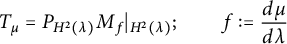 $$ \begin{align*}T _\mu = P_{H^2 (\lambda ) } M_{f} |_{H^2 (\lambda )}; \quad \quad f := \frac{d\mu}{d\lambda }\end{align*} $$
in the quadratic form sense, i.e.,
 $$ \begin{align*}\left\langle {\sqrt{T} _\mu p} , {\sqrt{T} _\mu q} \right\rangle_{H^2 (\lambda )} = \left\langle {M_{\sqrt{f}} \, p} , {M_{\sqrt{f}} \, q} \right\rangle_{L^2 (\lambda )}; \quad \quad \forall \ p, q \in \mathbb{C} [\zeta].\end{align*} $$
Proof Necessity was established in Proposition 4.4 and sufficiency, in the case where $\lambda $
is extreme, was proven in Proposition 4.6. To prove sufficiency in general, assume that
$\lambda $
is extreme, was proven in Proposition 4.6. To prove sufficiency in general, assume that $\mu \ll _{RK} \lambda $
so that the intersection space
$\mu \ll _{RK} \lambda $
so that the intersection space $\mathrm {int} (\mu , \lambda )$
is dense in the space of
$\mathrm {int} (\mu , \lambda )$
is dense in the space of $\mu $
-Cauchy transforms,
$\mu $
-Cauchy transforms, $\mathscr {H} ^+ (\mu )$
. Note that
$\mathscr {H} ^+ (\mu )$
. Note that $\mu \ll _{RK} \lambda $
if and only if
$\mu \ll _{RK} \lambda $
if and only if $\mu + \lambda \ll _{RK} \lambda $
(and the same is true for
$\mu + \lambda \ll _{RK} \lambda $
(and the same is true for $\ll $
). This follows from Aronszajn’s “sums of kernels” theorem as stated in Section 2.2. By Lemma 4.5,
$\ll $
). This follows from Aronszajn’s “sums of kernels” theorem as stated in Section 2.2. By Lemma 4.5, $\mathrm {e} _{\mu +\lambda , \lambda } : \mathrm {int} (\mu + \lambda , \lambda ) \subseteq \mathscr {H} ^+ (\mu +\lambda ) \hookrightarrow \mathscr {H} ^+ (\lambda )$
is a closed embedding,
$\mathrm {e} _{\mu +\lambda , \lambda } : \mathrm {int} (\mu + \lambda , \lambda ) \subseteq \mathscr {H} ^+ (\mu +\lambda ) \hookrightarrow \mathscr {H} ^+ (\lambda )$
is a closed embedding, $E_{\mu +\lambda , \lambda } := \mathscr {C} _{\mu +\lambda } ^* \mathrm {e} _{\mu +\lambda , \lambda } ^* \mathscr {C} _\lambda $
, is a closed co-embedding with
$E_{\mu +\lambda , \lambda } := \mathscr {C} _{\mu +\lambda } ^* \mathrm {e} _{\mu +\lambda , \lambda } ^* \mathscr {C} _\lambda $
, is a closed co-embedding with $\mathscr {K} _{\mathbb {D}} = \bigvee k_z$
and
$\mathscr {K} _{\mathbb {D}} = \bigvee k_z$
and $\mathbb {C} [\zeta ]$
as cores, and
$\mathbb {C} [\zeta ]$
as cores, and $T := T_{\mu +\lambda } = E_{\mu +\lambda , \lambda } ^* E_{\mu +\lambda , \lambda } \geq 0$
is self-adjoint, positive semi-definite, densely-defined, and
$T := T_{\mu +\lambda } = E_{\mu +\lambda , \lambda } ^* E_{\mu +\lambda , \lambda } \geq 0$
is self-adjoint, positive semi-definite, densely-defined, and $\lambda $
-Toeplitz.
$\lambda $
-Toeplitz.
By Remark 4.9 and Theorem 4.10 above, if $\hat {E} : L^2 (\mu + \lambda ) \hookrightarrow L^2 (\lambda )$
is the contractive co-embedding, and
$\hat {E} : L^2 (\mu + \lambda ) \hookrightarrow L^2 (\lambda )$
is the contractive co-embedding, and $\hat {T} := M_f$
, where
$\hat {T} := M_f$
, where $f \geq 0\ \lambda -a.e.$
,
$f \geq 0\ \lambda -a.e.$
, $f \in L^1 (\lambda )$
is the self-adjoint, positive semi-definite multiplication operator by the Radon–Nikodym derivative,
$f \in L^1 (\lambda )$
is the self-adjoint, positive semi-definite multiplication operator by the Radon–Nikodym derivative, ${f = \frac {d\mu }{d\lambda }}$
, then
${f = \frac {d\mu }{d\lambda }}$
, then $(I +\hat {T}) ^{-1} = \hat {E} \hat {E}^*$
. On the other hand,
$(I +\hat {T}) ^{-1} = \hat {E} \hat {E}^*$
. On the other hand, $E:= E_{\mu + \lambda , \lambda } : \mathrm {Dom} \, E_{\mu +\lambda , \lambda } \subseteq H^2 (\lambda ) \hookrightarrow H^2 (\mu +\lambda )$
is closed and bounded below by
$E:= E_{\mu + \lambda , \lambda } : \mathrm {Dom} \, E_{\mu +\lambda , \lambda } \subseteq H^2 (\lambda ) \hookrightarrow H^2 (\mu +\lambda )$
is closed and bounded below by $1$
, and so has a contractive inverse, namely, for any
$1$
, and so has a contractive inverse, namely, for any $h \in \mathscr {K} _{\mathbb {D}}$
or in
$h \in \mathscr {K} _{\mathbb {D}}$
or in $\mathbb {C} [\zeta ]$
,
$\mathbb {C} [\zeta ]$
,
 $$ \begin{align*}\hat{E} E h = h \in H^2 (\lambda ), \quad \mbox{and,} \quad E \hat{E} h = h \in H^2 (\mu +\lambda ).\end{align*} $$
Hence,
 $$ \begin{align*}\hat{E} E | _{\mathrm{Dom} \, E} = I_{H^2 (\lambda )} |_{\mathrm{Dom} \, E}, \quad \mbox{and} \quad E \hat{E} | _{H^2 (\mu + \lambda ) } = I _{\mu +\lambda }.\end{align*} $$
Observe that the contractive co-embedding, $\hat {E}$
is necessarily injective and has dense range, so that it has a closed, potentially unbounded inverse,
$\hat {E}$
is necessarily injective and has dense range, so that it has a closed, potentially unbounded inverse, $\hat {E} ^{-1}$
, which is densely-defined. Since
$\hat {E} ^{-1}$
, which is densely-defined. Since $(I +\hat {T} ) ^{-1} = \hat {E} \hat {E} ^*$
, we conclude that
$(I +\hat {T} ) ^{-1} = \hat {E} \hat {E} ^*$
, we conclude that $I +\hat {T} = \hat {E} ^{-*} \hat {E} ^{-1}$
. Hence, for any
$I +\hat {T} = \hat {E} ^{-*} \hat {E} ^{-1}$
. Hence, for any $p, q \in \mathbb {C} [\zeta ] \subseteq H^2 (\lambda )$
,
$p, q \in \mathbb {C} [\zeta ] \subseteq H^2 (\lambda )$
,
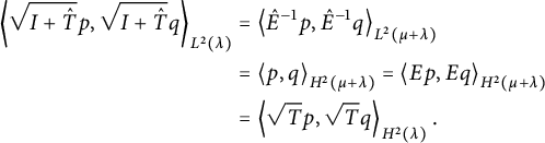 $$ \begin{align*} \left\langle {\sqrt{I +\hat{T}} p} , {\sqrt{I+ \hat{T}} q} \right\rangle_{L^2 (\lambda )} & = \left\langle {\hat{E} ^{-1} p} , {\hat{E} ^{-1} q} \right\rangle_{L^2 (\mu + \lambda )} \\ & = \left\langle {p} , {q} \right\rangle_{H^2 (\mu +\lambda )} = \left\langle {Ep} , {Eq} \right\rangle_{H^2 ( \mu +\lambda )} \\ & = \left\langle {\sqrt{T} p} , {\sqrt{T} q} \right\rangle_{H^2 (\lambda )}. \end{align*} $$
This calculation shows that the “compression” of $I + \hat {T}$
to the intersection of its domain with the subspace
$I + \hat {T}$
to the intersection of its domain with the subspace $H^2 (\lambda )$
is equal to T, in this quadratic form sense. In particular,
$H^2 (\lambda )$
is equal to T, in this quadratic form sense. In particular, ${T - I \geq 0}$
is the compression of
${T - I \geq 0}$
is the compression of $\hat {T} = M_f$
to
$\hat {T} = M_f$
to $H^2 (\lambda )$
, where
$H^2 (\lambda )$
, where $f \in L^1 (\lambda )$
is the Radon–Nikodym derivative of
$f \in L^1 (\lambda )$
is the Radon–Nikodym derivative of $\mu $
with respect to
$\mu $
with respect to $\lambda $
. In conclusion, for any polynomials
$\lambda $
. In conclusion, for any polynomials $p,q$
,
$p,q$
,
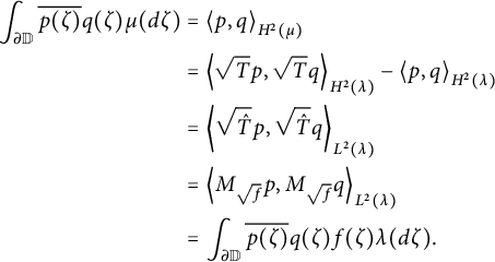 $$ \begin{align*} \int _{\partial \mathbb{D}} \overline{p(\zeta)} q (\zeta) \mu (d\zeta ) & = \left\langle {p} , {q} \right\rangle_{H^2 (\mu )} \\ & = \left\langle {\sqrt{T}p} , {\sqrt{T}q} \right\rangle_{H^2 (\lambda )} - \left\langle {p} , {q} \right\rangle_{H^2 (\lambda )} \\ & = \left\langle {\sqrt{\hat{T}} p} , {\sqrt{\hat{T}}q} \right\rangle_{L^2 (\lambda )} \\ & = \left\langle {M_{\sqrt{f}} p} , {M_{\sqrt{f}} q} \right\rangle_{L^2 (\lambda )} \\ & = \int _{\partial \mathbb{D}} \overline{p(\zeta)} q(\zeta) f (\zeta ) \lambda (d\zeta ). \end{align*} $$
As in the second proof of sufficiency of Theorem 4.1, this equality can be extended to arbitrary $g,h \in \mathbb {C} [\zeta ] + \overline {\mathbb {C} [\zeta ] }$
, so that by Weierstraß approximation,
$g,h \in \mathbb {C} [\zeta ] + \overline {\mathbb {C} [\zeta ] }$
, so that by Weierstraß approximation, $\mu \ll \lambda $
with Radon–Nikodym derivative
$\mu \ll \lambda $
with Radon–Nikodym derivative $f \geq 0$
,
$f \geq 0$
, $f \in L^1 (\lambda )$
.
$f \in L^1 (\lambda )$
.
5 Lebesgue decomposition via reproducing kernels
By Theorem 4.12, our definition of reproducing kernel absolute continuity is equivalent to the classical definition of absolute continuity for finite, positive, and regular Borel measures on the complex unit circle. In particular, if $\mu \ll \lambda $
, it follows that the intersection space of
$\mu \ll \lambda $
, it follows that the intersection space of $\mu $
and
$\mu $
and $\lambda $
-Cauchy transforms is dense in the space of
$\lambda $
-Cauchy transforms is dense in the space of $\mu $
-Cauchy transforms. Hence, if
$\mu $
-Cauchy transforms. Hence, if $\mu = \mu _{ac} + \mu _s$
is the Lebesgue decomposition of
$\mu = \mu _{ac} + \mu _s$
is the Lebesgue decomposition of $\mu $
with respect to
$\mu $
with respect to $\lambda $
, then
$\lambda $
, then $\mathrm {int} (\mu _{ac} , \lambda )$
is dense in
$\mathrm {int} (\mu _{ac} , \lambda )$
is dense in $\mathscr {H} ^+ (\mu _{ac} )$
, and since
$\mathscr {H} ^+ (\mu _{ac} )$
, and since $\mu \geq \mu _{ac}$
,
$\mu \geq \mu _{ac}$
, $\mathrm {int} (\mu _{ac} , \lambda ) \subseteq \mathrm {int} (\mu , \lambda )$
. That is, if
$\mathrm {int} (\mu _{ac} , \lambda ) \subseteq \mathrm {int} (\mu , \lambda )$
. That is, if $\mu _{ac} \neq 0$
, it follows that
$\mu _{ac} \neq 0$
, it follows that $\mathrm {int} (\mu , \lambda ) \neq \{ 0 \}$
is not trivial. This raises several natural questions: How can we identify the space of
$\mathrm {int} (\mu , \lambda ) \neq \{ 0 \}$
is not trivial. This raises several natural questions: How can we identify the space of $\mu _{ac}$
-Cauchy transforms? Is
$\mu _{ac}$
-Cauchy transforms? Is $\mathrm {int} (\mu , \lambda ) ^{-\mu } := \mathrm {int} (\mu , \lambda ) ^{ -\| \cdot \| _{\mu } }$
equal to the space of
$\mathrm {int} (\mu , \lambda ) ^{-\mu } := \mathrm {int} (\mu , \lambda ) ^{ -\| \cdot \| _{\mu } }$
equal to the space of $\mu _{ac}$
-Cauchy transforms? We will see that the answer to the second question is positive if
$\mu _{ac}$
-Cauchy transforms? We will see that the answer to the second question is positive if $\lambda $
is non-extreme, but that in general,
$\lambda $
is non-extreme, but that in general, $\mathrm {int} (\mu , \lambda ) ^{-\mu }$
is not the space of Cauchy transforms of any positive measure (see Corollary 5.15 and Example 5.17).
$\mathrm {int} (\mu , \lambda ) ^{-\mu }$
is not the space of Cauchy transforms of any positive measure (see Corollary 5.15 and Example 5.17).
Theorem 5.1 If $\mathscr {M}$
is a RKHS in
$\mathscr {M}$
is a RKHS in $\mathbb {D}$
that embeds contractively in
$\mathbb {D}$
that embeds contractively in $\mathscr {H} ^+ (\mu )$
, then
$\mathscr {H} ^+ (\mu )$
, then $\mathscr {M} = \mathscr {H} ^+ (\gamma )$
for a positive measure,
$\mathscr {M} = \mathscr {H} ^+ (\gamma )$
for a positive measure, $\gamma $
,
$\gamma $
, $\gamma \leq \mu $
, if and only if
$\gamma \leq \mu $
, if and only if $\mathrm {e} : \mathscr {M} \hookrightarrow \mathscr {H} ^+ (\mu )$
is such that the positive semi-definite contraction
$\mathrm {e} : \mathscr {M} \hookrightarrow \mathscr {H} ^+ (\mu )$
is such that the positive semi-definite contraction $\tau := \mathrm {e} \mathrm {e} ^*$
is
$\tau := \mathrm {e} \mathrm {e} ^*$
is $V_\mu $
-Toeplitz.
$V_\mu $
-Toeplitz.
In this case, $\mathscr {M} = \mathscr {H} ^+ (\gamma ) = \mathscr {R} (\mathrm {e} )$
, and the complementary space of
$\mathscr {M} = \mathscr {H} ^+ (\gamma ) = \mathscr {R} (\mathrm {e} )$
, and the complementary space of $\mathscr {H} ^+ (\gamma )$
in
$\mathscr {H} ^+ (\gamma )$
in $\mathscr {H} ^+ (\mu )$
is
$\mathscr {H} ^+ (\mu )$
is $\mathscr {H} ^+ (\nu )$
, for a positive measure,
$\mathscr {H} ^+ (\nu )$
, for a positive measure, $\nu $
, where
$\nu $
, where $k^\nu = k^\mu - k^\gamma $
so that
$k^\nu = k^\mu - k^\gamma $
so that $\mu = \gamma + \nu $
.
$\mu = \gamma + \nu $
.
Proof First, if $\mathscr {H} ^+ (\gamma ) = \mathscr {M} \subseteq \mathscr {H} ^+ (\mu )$
is contractively contained, then,
$\mathscr {H} ^+ (\gamma ) = \mathscr {M} \subseteq \mathscr {H} ^+ (\mu )$
is contractively contained, then, $\mathrm {e} : \mathscr {H} ^+ (\gamma ) \hookrightarrow \mathscr {H} ^+ (\mu )$
is trivially a (contractive) multiplier so that, as before,
$\mathrm {e} : \mathscr {H} ^+ (\gamma ) \hookrightarrow \mathscr {H} ^+ (\mu )$
is trivially a (contractive) multiplier so that, as before, $\mathrm {e} ^* k_z ^\mu = k_z ^\gamma $
, and
$\mathrm {e} ^* k_z ^\mu = k_z ^\gamma $
, and
 $$ \begin{align*}\mathrm{e} ^* V^\mu = V^\gamma \mathrm{e} ^*.\end{align*} $$
In conclusion,
 $$ \begin{align*}V ^{\mu *} \mathrm{e} \mathrm{e} ^* V^\mu = \mathrm{e} V ^{\gamma *} V^\gamma \mathrm{e} ^* = \mathrm{e} \mathrm{e} ^* = \tau.\end{align*} $$
Conversely, if $\tau = \mathrm {e} \mathrm {e} ^*$
is
$\tau = \mathrm {e} \mathrm {e} ^*$
is $V^\mu $
-Toeplitz and contractive, then, as in the proof of Theorem 4.1,
$V^\mu $
-Toeplitz and contractive, then, as in the proof of Theorem 4.1, $T := \mathscr {C} _\mu ^* \mathrm {e} \mathrm {e} ^* \mathscr {C} _\mu $
is a contractive
$T := \mathscr {C} _\mu ^* \mathrm {e} \mathrm {e} ^* \mathscr {C} _\mu $
is a contractive $Z ^\mu $
-Toeplitz operator and we can appeal to the Riesz–Markov theorem to show that there is a
$Z ^\mu $
-Toeplitz operator and we can appeal to the Riesz–Markov theorem to show that there is a $\gamma \geq 0$
, so that
$\gamma \geq 0$
, so that $T = P_{H^2 (\mu )} M_f | _{H^2 (\mu )}$
, where
$T = P_{H^2 (\mu )} M_f | _{H^2 (\mu )}$
, where $f \geq 0$
,
$f \geq 0$
, $\| f \| _\infty \leq 1$
is the Radon–Nikodym derivative of
$\| f \| _\infty \leq 1$
is the Radon–Nikodym derivative of $\gamma $
with respect to
$\gamma $
with respect to $\mu $
. Namely, one can define a linear functional,
$\mu $
. Namely, one can define a linear functional, $\hat {\mu } _T$
, on
$\hat {\mu } _T$
, on $\mathbb {C} [\zeta ] + \overline {\mathbb {C} [\zeta ]} \subseteq \mathscr {C} (\partial \mathbb {D} )$
, by
$\mathbb {C} [\zeta ] + \overline {\mathbb {C} [\zeta ]} \subseteq \mathscr {C} (\partial \mathbb {D} )$
, by
 $$ \begin{align*}\hat{\mu} _T (p + \overline{q} ) := \left\langle {1} , {Tp} \right\rangle_{H^2 (\mu )} + \left\langle {q} , {T1} \right\rangle_{H^2 (\mu )}.\end{align*} $$
It is easy to check that $\hat {\mu } _T$
is bounded and positive using the Fejér–Riesz theorem, as in the proof of Theorem 4.1. The fact that T is a positive semi-definite
$\hat {\mu } _T$
is bounded and positive using the Fejér–Riesz theorem, as in the proof of Theorem 4.1. The fact that T is a positive semi-definite $Z^\mu $
-Toeplitz contraction ensures that
$Z^\mu $
-Toeplitz contraction ensures that $\hat {\mu } _T$
extends to a bounded, positive linear functional on
$\hat {\mu } _T$
extends to a bounded, positive linear functional on $\mathscr {C} (\partial \mathbb {D} )$
, and that
$\mathscr {C} (\partial \mathbb {D} )$
, and that $\hat {\mu } _T \leq \hat {\mu }$
, so that
$\hat {\mu } _T \leq \hat {\mu }$
, so that $\hat {\mu } _T = \hat {\gamma }$
for some finite, regular, and positive Borel measure,
$\hat {\mu } _T = \hat {\gamma }$
for some finite, regular, and positive Borel measure, $\gamma \leq \mu $
, by the Riesz–Markov theorem.
$\gamma \leq \mu $
, by the Riesz–Markov theorem.
By Theorem 2.4, the complementary space, $\mathscr {R} ^c (\mathrm {e} )$
, of
$\mathscr {R} ^c (\mathrm {e} )$
, of $\mathscr {R} (\mathrm {e}) = \mathscr {H} ^+ (\gamma )$
is a RKHS in
$\mathscr {R} (\mathrm {e}) = \mathscr {H} ^+ (\gamma )$
is a RKHS in $\mathbb {D}$
with reproducing kernel
$\mathbb {D}$
with reproducing kernel $k ' (z,w) = k^\mu (z,w) - k^\gamma (z,w)$
and it is contractively contained in
$k ' (z,w) = k^\mu (z,w) - k^\gamma (z,w)$
and it is contractively contained in $\mathscr {H} ^+ (\mu )$
, by the inclusion theorem. Moreover, if
$\mathscr {H} ^+ (\mu )$
, by the inclusion theorem. Moreover, if $\mathrm {j} : \mathscr {R} ^c (\mathrm {e} ) \hookrightarrow \mathscr {H} ^+ (\mu )$
is the contractive embedding, then it follows that
$\mathrm {j} : \mathscr {R} ^c (\mathrm {e} ) \hookrightarrow \mathscr {H} ^+ (\mu )$
is the contractive embedding, then it follows that $\mathrm {j} \mathrm {j} ^* = I - \mathrm {e} \mathrm {e} ^* \geq 0$
is also a positive semi-definite
$\mathrm {j} \mathrm {j} ^* = I - \mathrm {e} \mathrm {e} ^* \geq 0$
is also a positive semi-definite $V^\mu $
-Toeplitz contraction. Hence, by the first part of the proof,
$V^\mu $
-Toeplitz contraction. Hence, by the first part of the proof, $\mathscr {H} = \mathscr {H} ^+ (\nu )$
for a positive measure,
$\mathscr {H} = \mathscr {H} ^+ (\nu )$
for a positive measure, $\nu $
. Finally, since
$\nu $
. Finally, since $k^\mu = k^\gamma + k^\nu $
, we obtain that
$k^\mu = k^\gamma + k^\nu $
, we obtain that $\mu = \gamma + \nu $
.
$\mu = \gamma + \nu $
.
Lemma 5.2 Given any $\mu , \lambda $
, the intersection space
$\mu , \lambda $
, the intersection space $\mathrm {int} (\mu ,\lambda )$
, is both
$\mathrm {int} (\mu ,\lambda )$
, is both $V_\lambda $
and
$V_\lambda $
and $V_\mu $
-co-invariant, and
$V_\mu $
-co-invariant, and $V_\lambda ^* | _{\mathrm {int} (\mu , \lambda )} = V_\mu ^* |_{\mathrm {int} (\mu , \lambda )}$
.
$V_\lambda ^* | _{\mathrm {int} (\mu , \lambda )} = V_\mu ^* |_{\mathrm {int} (\mu , \lambda )}$
.
Proof This is immediate, by Lemma 3.4, since both $V_\mu ^*$
and
$V_\mu ^*$
and $V_\lambda ^*$
act as “backward shifts” on power series.
$V_\lambda ^*$
act as “backward shifts” on power series.
Lemma 5.3 If $\lambda $
is non-extreme, then the intersection space,
$\lambda $
is non-extreme, then the intersection space, $\mathrm {int} (\mu , \lambda )$
, is
$\mathrm {int} (\mu , \lambda )$
, is $V_\mu $
-reducing. If
$V_\mu $
-reducing. If $\lambda $
is extreme, then
$\lambda $
is extreme, then $\mathrm {int} (\mu , \lambda )$
is
$\mathrm {int} (\mu , \lambda )$
is $V_\mu $
-reducing (and
$V_\mu $
-reducing (and $V_\lambda $
-reducing) if and only if
$V_\lambda $
-reducing) if and only if $V_{\mu } | _{\mathrm {int} (\mu , \lambda )} = V_\lambda | _{\mathrm {int} (\mu , \lambda )}$
.
$V_{\mu } | _{\mathrm {int} (\mu , \lambda )} = V_\lambda | _{\mathrm {int} (\mu , \lambda )}$
.
Proof By Lemma 3.4, if $h \in \mathrm {int} (\mu , \lambda )$
, then
$h \in \mathrm {int} (\mu , \lambda )$
, then $V_\mu h \in \mathscr {H} ^+ (\mu )$
and
$V_\mu h \in \mathscr {H} ^+ (\mu )$
and
 $$ \begin{align} (V_\mu h) (z) = z h(z) + (V_\mu h) (0) 1= (V_\lambda h) (z) - (V_\lambda h) (0) 1 + (V_\mu h) (0) 1. \end{align} $$
Hence, if $c:= (V_\lambda h) (0) - (V_\mu h) (0) \in \mathbb {C}$
and
$c:= (V_\lambda h) (0) - (V_\mu h) (0) \in \mathbb {C}$
and $\lambda $
is non-extreme, then both
$\lambda $
is non-extreme, then both $V_\lambda h$
and
$V_\lambda h$
and $c1$
belong to
$c1$
belong to $\mathscr {H} ^+ (\lambda )$
so that
$\mathscr {H} ^+ (\lambda )$
so that $V_\mu h \in \mathscr {H} ^+ (\lambda ) \cap \mathscr {H} ^+ (\mu ) = \mathrm {int} (\mu , \lambda )$
. Recall that
$V_\mu h \in \mathscr {H} ^+ (\lambda ) \cap \mathscr {H} ^+ (\mu ) = \mathrm {int} (\mu , \lambda )$
. Recall that $\lambda $
is extreme if and only if
$\lambda $
is extreme if and only if $\mathscr {H} ^+ (\lambda )$
does not contain the constant functions. Hence, if
$\mathscr {H} ^+ (\lambda )$
does not contain the constant functions. Hence, if $\lambda $
is extreme then
$\lambda $
is extreme then $\mathrm {int} (\mu ,\lambda )$
will be
$\mathrm {int} (\mu ,\lambda )$
will be $V_\mu $
-reducing if and only if
$V_\mu $
-reducing if and only if $(V_\mu h) (0) = (V_\lambda h) (0)$
for all
$(V_\mu h) (0) = (V_\lambda h) (0)$
for all $h \in \mathrm {int} (\mu , \lambda )$
. By Equation (5.1), this happens if and only if
$h \in \mathrm {int} (\mu , \lambda )$
. By Equation (5.1), this happens if and only if $V_\mu h = V_\lambda h$
.
$V_\mu h = V_\lambda h$
.
Corollary 5.4 If $\mathscr {M} \subseteq \mathscr {H} ^+ (\mu )$
is a
$\mathscr {M} \subseteq \mathscr {H} ^+ (\mu )$
is a $V_\mu $
-reducing subspace, then
$V_\mu $
-reducing subspace, then $\mathscr {M} = \mathscr {H} ^+ (\gamma )$
for some
$\mathscr {M} = \mathscr {H} ^+ (\gamma )$
for some $\gamma \leq \mu $
. Moreover,
$\gamma \leq \mu $
. Moreover, $\mathscr {M} ^\perp = \mathscr {H} ^+ (\gamma ')$
for some
$\mathscr {M} ^\perp = \mathscr {H} ^+ (\gamma ')$
for some $\mu \geq \gamma ' \geq 0$
so that
$\mu \geq \gamma ' \geq 0$
so that $\gamma + \gamma ' = \mu $
.
$\gamma + \gamma ' = \mu $
.
Proof Let P be the orthogonal projection of $\mathscr {H} ^+ (\mu )$
onto
$\mathscr {H} ^+ (\mu )$
onto $\mathscr {M}$
. Then if
$\mathscr {M}$
. Then if $\mathrm {e} : \mathscr {M} \hookrightarrow \mathscr {H} ^+ (\mu )$
is the isometric embedding,
$\mathrm {e} : \mathscr {M} \hookrightarrow \mathscr {H} ^+ (\mu )$
is the isometric embedding, $P= \mathrm {e} \mathrm {e} ^*$
. Hence,
$P= \mathrm {e} \mathrm {e} ^*$
. Hence,
 $$ \begin{align*}V_\mu ^* \mathrm{e} \mathrm{e} ^* V_\mu = V_\mu ^* P V_\mu = V_\mu ^* V_\mu P = P = \mathrm{e}\mathrm{e} ^*,\end{align*} $$
so that $\tau = \mathrm {e} \mathrm {e} ^*$
is
$\tau = \mathrm {e} \mathrm {e} ^*$
is $V ^\mu $
-Toeplitz and
$V ^\mu $
-Toeplitz and $\mathscr {M} = \mathscr {H} ^+ (\gamma )$
for some
$\mathscr {M} = \mathscr {H} ^+ (\gamma )$
for some $0 \leq \gamma \leq \mu $
, and
$0 \leq \gamma \leq \mu $
, and $\mathscr {M} ^\perp = \mathscr {H} ^+ (\gamma ' )$
, by Theorem 5.1.
$\mathscr {M} ^\perp = \mathscr {H} ^+ (\gamma ' )$
, by Theorem 5.1.
Theorem 5.5 Let $\mu , \lambda \geq 0$
be finite, positive, and regular Borel measures on
$\mu , \lambda \geq 0$
be finite, positive, and regular Borel measures on $\partial \mathbb {D}$
. If the intersection space,
$\partial \mathbb {D}$
. If the intersection space, $\mathrm {int} (\mu , \lambda )$
, is
$\mathrm {int} (\mu , \lambda )$
, is $V ^\mu $
-reducing and
$V ^\mu $
-reducing and $\mu = \mu _{ac} + \mu _s$
is the Lebesgue decomposition of
$\mu = \mu _{ac} + \mu _s$
is the Lebesgue decomposition of $\mu $
with respect to
$\mu $
with respect to $\lambda $
, then
$\lambda $
, then
 $$ \begin{align*}\mathscr{H} ^+ (\mu ) = \mathscr{H} ^+ ( \mu _{ac} ) \oplus \mathscr{H} ^+ (\mu _s ).\end{align*} $$
In this case,
 $$ \begin{align*}\mathscr{H} ^+ (\mu _{ac} ) = \mathrm{int} (\mu , \lambda ) ^{-\mu}, \quad \mbox{and} \quad \mathscr{H} ^+ (\mu _s ) \cap \mathscr{H} ^+ (\lambda ) = \{ 0 \}.\end{align*} $$
That is, $\mu _{ac}$
is the largest positive measure
$\mu _{ac}$
is the largest positive measure $\leq \mu $
which is RK-ac with respect to
$\leq \mu $
which is RK-ac with respect to $\lambda $
, and
$\lambda $
, and $\mu _s$
is RK-singular with respect to
$\mu _s$
is RK-singular with respect to $\lambda $
.
$\lambda $
.
In particular, $\mathrm {int} (\mu , \lambda )$
will be
$\mathrm {int} (\mu , \lambda )$
will be $V^\mu $
-reducing if
$V^\mu $
-reducing if $\lambda $
is non-extreme by Lemma 5.3.
$\lambda $
is non-extreme by Lemma 5.3.
Proof By Theorem 4.12, we have that $\mathrm {int} (\mu _{ac}, \lambda ) \subseteq \mathrm {int} (\mu , \lambda )$
is dense in
$\mathrm {int} (\mu _{ac}, \lambda ) \subseteq \mathrm {int} (\mu , \lambda )$
is dense in $\mathscr {H} ^+ (\mu _{ac})$
. Since we assume that
$\mathscr {H} ^+ (\mu _{ac})$
. Since we assume that $\mathrm {int} (\mu , \lambda )$
is
$\mathrm {int} (\mu , \lambda )$
is $V_\mu $
-reducing, its closure,
$V_\mu $
-reducing, its closure, $\mathrm {int} (\mu , \lambda ) ^{-\mu }$
, is also
$\mathrm {int} (\mu , \lambda ) ^{-\mu }$
, is also $V_\mu $
-reducing and then
$V_\mu $
-reducing and then $\mathrm {int} (\mu , \lambda ) ^{-\mu } = \mathscr {H} ^+ (\gamma )$
for some
$\mathrm {int} (\mu , \lambda ) ^{-\mu } = \mathscr {H} ^+ (\gamma )$
for some $0 \leq \gamma \leq \mu $
by Corollary 5.4. By construction
$0 \leq \gamma \leq \mu $
by Corollary 5.4. By construction $\gamma \ll _{RK} \lambda $
so that
$\gamma \ll _{RK} \lambda $
so that $\gamma \ll \lambda $
by Theorem 4.12. By maximality,
$\gamma \ll \lambda $
by Theorem 4.12. By maximality, $\gamma \leq \mu _{ac}$
and by construction
$\gamma \leq \mu _{ac}$
and by construction $\mathrm {int} (\mu , \lambda ) \subseteq \mathrm {int} (\gamma , \lambda )$
. However, we also have that
$\mathrm {int} (\mu , \lambda ) \subseteq \mathrm {int} (\gamma , \lambda )$
. However, we also have that $\mathrm {int} (\mu _{ac} , \lambda ) \subseteq \mathrm {int} (\mu , \lambda ) \subseteq \mathrm {int} (\gamma , \lambda )$
. Hence, if
$\mathrm {int} (\mu _{ac} , \lambda ) \subseteq \mathrm {int} (\mu , \lambda ) \subseteq \mathrm {int} (\gamma , \lambda )$
. Hence, if $\mathrm {e} : \mathscr {H} ^+ (\mu _{ac} ) \hookrightarrow \mathscr {H} ^+ (\mu )$
is the contractive embedding, then
$\mathrm {e} : \mathscr {H} ^+ (\mu _{ac} ) \hookrightarrow \mathscr {H} ^+ (\mu )$
is the contractive embedding, then $\mathrm {e}$
, restricted to the dense subspace
$\mathrm {e}$
, restricted to the dense subspace $\mathrm {int} (\mu _{ac} , \lambda ) \subseteq \mathscr {H} ^+ (\mu _{ac} )$
defines a contraction into
$\mathrm {int} (\mu _{ac} , \lambda ) \subseteq \mathscr {H} ^+ (\mu _{ac} )$
defines a contraction into $\mathscr {H} ^+ (\gamma )$
, which is isometrically contained in
$\mathscr {H} ^+ (\gamma )$
, which is isometrically contained in $\mathscr {H} ^+ (\mu )$
. It follows that
$\mathscr {H} ^+ (\mu )$
. It follows that $\mathrm {e}$
extends by continuity to a contractive embedding of
$\mathrm {e}$
extends by continuity to a contractive embedding of $\mathscr {H} ^+ (\mu _{ac} )$
into
$\mathscr {H} ^+ (\mu _{ac} )$
into $\mathscr {H} ^+ (\gamma )$
. Hence, by Theorem 4.1,
$\mathscr {H} ^+ (\gamma )$
. Hence, by Theorem 4.1, $\mu _{ac} \leq \gamma $
and we conclude that
$\mu _{ac} \leq \gamma $
and we conclude that $\mu _{ac} =\gamma $
.
$\mu _{ac} =\gamma $
.
Corollary 5.6 Let $\mu , \lambda \geq 0$
be finite, positive, and regular Borel measures on
$\mu , \lambda \geq 0$
be finite, positive, and regular Borel measures on $\partial \mathbb {D}$
. If
$\partial \mathbb {D}$
. If $\mathrm {int} (\mu ,\lambda ) = \{ 0 \}$
so that
$\mathrm {int} (\mu ,\lambda ) = \{ 0 \}$
so that $\mu \perp _{RK} \lambda $
, then
$\mu \perp _{RK} \lambda $
, then $\mu \perp \lambda $
. If
$\mu \perp \lambda $
. If $\mathrm {int} (\mu , \lambda )$
is either
$\mathrm {int} (\mu , \lambda )$
is either $V_\mu $
or
$V_\mu $
or $V_\lambda $
-reducing then
$V_\lambda $
-reducing then $\mu \perp \lambda $
if and only if
$\mu \perp \lambda $
if and only if $\mu \perp _{RK} \lambda $
. In particular, if either
$\mu \perp _{RK} \lambda $
. In particular, if either $\mu $
or
$\mu $
or $\lambda $
is non-extreme then
$\lambda $
is non-extreme then $\mu \perp \lambda $
if and only if
$\mu \perp \lambda $
if and only if $\mu \perp _{RK} \lambda $
.
$\mu \perp _{RK} \lambda $
.
While the previous two results give quite a satisfactory description of the Lebesgue decomposition of $\mu $
with respect to
$\mu $
with respect to $\lambda $
in terms of reproducing kernel theory in the case where the intersection space,
$\lambda $
in terms of reproducing kernel theory in the case where the intersection space, $\mathrm {int} (\mu ,\lambda )$
is
$\mathrm {int} (\mu ,\lambda )$
is $V^\mu $
-reducing, this is not generally the case, as the next proposition and example show.
$V^\mu $
-reducing, this is not generally the case, as the next proposition and example show.
In the proposition statement below, recall the definition of the lattice operations $\vee , \wedge $
on positive kernels and the definition of the isometries
$\vee , \wedge $
on positive kernels and the definition of the isometries $U_\vee : \mathcal {H} (K +k ) \rightarrow \mathcal {H} (K) \oplus \mathcal {H} (k)$
and
$U_\vee : \mathcal {H} (K +k ) \rightarrow \mathcal {H} (K) \oplus \mathcal {H} (k)$
and $U_\wedge : \mathcal {H} (K \wedge k) = \mathcal {H} (K) \cap \mathcal {H} (k) \rightarrow \mathcal {H} (K) \oplus \mathcal {H} (k)$
(see Section 2.2).
$U_\wedge : \mathcal {H} (K \wedge k) = \mathcal {H} (K) \cap \mathcal {H} (k) \rightarrow \mathcal {H} (K) \oplus \mathcal {H} (k)$
(see Section 2.2).
Proposition 5.7 If $\mu + \lambda $
is extreme, then
$\mu + \lambda $
is extreme, then $\mathrm {int} (\mu , \lambda )$
is
$\mathrm {int} (\mu , \lambda )$
is $V_\mu $
-reducing. If
$V_\mu $
-reducing. If $\mu , \lambda $
are both extreme but
$\mu , \lambda $
are both extreme but $\mu + \lambda $
is non-extreme, then
$\mu + \lambda $
is non-extreme, then $\mathrm {int} (\mu , \lambda )$
is nontrivial, but not
$\mathrm {int} (\mu , \lambda )$
is nontrivial, but not $V_\mu $
-reducing and
$V_\mu $
-reducing and
 $$ \begin{align*}\mathrm{int} (\mu , \lambda ) \supseteq U_\wedge ^* \bigvee _{j=1} ^\infty (V_\mu ^* \oplus V_\lambda ^* ) ^j U_\vee 1.\end{align*} $$
Lemma 5.8 Let $\mu , \lambda \geq 0$
be positive, finite, and regular Borel measures on
$\mu , \lambda \geq 0$
be positive, finite, and regular Borel measures on $\partial \mathbb {D}$
. Consider the RKHSs of
$\partial \mathbb {D}$
. Consider the RKHSs of $\mu , \lambda $
, and
$\mu , \lambda $
, and $\mu + \lambda $
-Cauchy transforms in
$\mu + \lambda $
-Cauchy transforms in $\partial \mathbb {D}$
,
$\partial \mathbb {D}$
, $\mathscr {H} ^+ (\mu ) = \mathcal {H} (k^\mu )$
,
$\mathscr {H} ^+ (\mu ) = \mathcal {H} (k^\mu )$
, $\mathscr {H} ^+ (\lambda ) = \mathcal {H} (k ^\lambda ),$
and
$\mathscr {H} ^+ (\lambda ) = \mathcal {H} (k ^\lambda ),$
and $\mathscr {H} ^+ (\mu + \lambda ) = \mathcal {H} ( k^\mu + k^\lambda )$
. Then,
$\mathscr {H} ^+ (\mu + \lambda ) = \mathcal {H} ( k^\mu + k^\lambda )$
. Then,
 $$ \begin{align*}U_\vee V_{\mu + \lambda } = V_\mu \oplus V_\lambda U_\vee\end{align*} $$
and $\mathrm {Ran} \, U_\vee $
is
$\mathrm {Ran} \, U_\vee $
is $V_\mu \oplus V_\lambda $
-invariant so that
$V_\mu \oplus V_\lambda $
-invariant so that $\mathrm {Ran} \, U_\wedge $
is
$\mathrm {Ran} \, U_\wedge $
is $V_\mu \oplus V_\lambda $
co-invariant, and
$V_\mu \oplus V_\lambda $
co-invariant, and
 $$ \begin{align*}U_\wedge V^{\mu *} | _{\mathrm{int} (\mu, \lambda )} = U_\wedge V^{\lambda *} |_{\mathrm{int} (\mu, \lambda )} = (V^\mu \oplus V^\lambda ) ^* U_\wedge.\end{align*} $$
Moreover, we have that $V_\mu | _{\mathrm {int} (\mu , \lambda )} = V_\lambda | _{\mathrm {int} (\mu , \lambda )}$
so that
$V_\mu | _{\mathrm {int} (\mu , \lambda )} = V_\lambda | _{\mathrm {int} (\mu , \lambda )}$
so that $\mathrm {int} (\mu , \lambda ) = \mathcal {H} (k^\mu \wedge k^\lambda )$
is both
$\mathrm {int} (\mu , \lambda ) = \mathcal {H} (k^\mu \wedge k^\lambda )$
is both $V_\mu $
and
$V_\mu $
and $V_\lambda $
-invariant if and only if
$V_\lambda $
-invariant if and only if $\mathrm {Ran} \, U_\wedge $
is
$\mathrm {Ran} \, U_\wedge $
is $V_\mu \oplus V_\lambda $
-invariant.
$V_\mu \oplus V_\lambda $
-invariant.
Proof The intertwining formulas are easily verified. The range of $U _\wedge : \mathscr {H} ^+ (\mu + \lambda ) \rightarrow \mathscr {H} ^+ (\mu ) \oplus \mathscr {H} ^+ (\lambda )$
is
$U _\wedge : \mathscr {H} ^+ (\mu + \lambda ) \rightarrow \mathscr {H} ^+ (\mu ) \oplus \mathscr {H} ^+ (\lambda )$
is $V_\mu \oplus V_\lambda $
-reducing if and only if, for any
$V_\mu \oplus V_\lambda $
-reducing if and only if, for any $h \oplus -h \in \mathrm {Ran} \, U _\wedge $
,
$h \oplus -h \in \mathrm {Ran} \, U _\wedge $
, $h \in \mathrm {int} (\mu , \lambda )$
,
$h \in \mathrm {int} (\mu , \lambda )$
,
 $$ \begin{align*}V _\mu h \oplus - V_\lambda h = g \oplus -g,\end{align*} $$
for some $g \in \mathrm {int} (\mu , \lambda )$
. Clearly, this happens if and only if
$g \in \mathrm {int} (\mu , \lambda )$
. Clearly, this happens if and only if $V_\mu | _{\mathrm {int} (\mu , \lambda )} = V_\lambda | _{\mathrm {int} (\mu , \lambda )}$
.
$V_\mu | _{\mathrm {int} (\mu , \lambda )} = V_\lambda | _{\mathrm {int} (\mu , \lambda )}$
.
Proof of Proposition 5.7
If $\lambda + \mu $
is extreme, then
$\lambda + \mu $
is extreme, then $\mathscr {H} ^+ (\mu + \lambda ) = \mathscr {H} ^+ (\mu ) + \mathscr {H} ^+ (\lambda )$
does not contain the constant functions. Hence, both
$\mathscr {H} ^+ (\mu + \lambda ) = \mathscr {H} ^+ (\mu ) + \mathscr {H} ^+ (\lambda )$
does not contain the constant functions. Hence, both $\lambda $
and
$\lambda $
and $\mu $
must also be extreme. In this case,
$\mu $
must also be extreme. In this case, $V_\mu , V_\lambda $
, and
$V_\mu , V_\lambda $
, and $V_{\mu + \lambda }$
are all unitary operators. We know that
$V_{\mu + \lambda }$
are all unitary operators. We know that $\mathrm {Ran} \, U_\vee $
is always
$\mathrm {Ran} \, U_\vee $
is always $V_\mu \oplus V_\lambda $
-invariant. On the other hand, since
$V_\mu \oplus V_\lambda $
-invariant. On the other hand, since $\mu + \lambda $
is extreme,
$\mu + \lambda $
is extreme, $V_{\mu + \lambda }$
is unitary, hence surjective, and
$V_{\mu + \lambda }$
is unitary, hence surjective, and
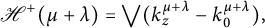 $$ \begin{align*}\mathscr{H} ^+ ( \mu + \lambda ) = \bigvee (k_z ^{\mu +\lambda } - k_0 ^{\mu + \lambda } ),\end{align*} $$
so that
 $$ \begin{align*}\mathrm{Ran} \, U_\vee = \bigvee (k_z ^{\mu} - k_0 ^{\mu} ) \oplus (k_z ^\lambda - k_0 ^\lambda ).\end{align*} $$
Hence,
 $$ \begin{align*}(V_\mu ^* \oplus V_\lambda ^*) \mathrm{Ran} \, U_\vee = \bigvee k_z ^\mu \overline{z} \oplus k_z ^\lambda \overline{z} \subseteq \mathrm{Ran} \, U_\vee.\end{align*} $$
It follows that $\mathrm {Ran} \, U_\vee $
is
$\mathrm {Ran} \, U_\vee $
is $V_\mu \oplus V_\lambda $
-reducing, so that
$V_\mu \oplus V_\lambda $
-reducing, so that $\mathrm {Ran} \, U_\wedge = \mathrm {Ran} \, U_\vee ^\perp $
is also reducing. The previous lemma now implies that
$\mathrm {Ran} \, U_\wedge = \mathrm {Ran} \, U_\vee ^\perp $
is also reducing. The previous lemma now implies that $\mathrm {int} (\mu , \lambda )$
is
$\mathrm {int} (\mu , \lambda )$
is $V_\mu $
-reducing.
$V_\mu $
-reducing.
If, on the other hand, $\mu , \lambda $
are both extreme but
$\mu , \lambda $
are both extreme but $\mu + \lambda $
is not, then
$\mu + \lambda $
is not, then $V^\mu , V^\lambda $
are both unitary but
$V^\mu , V^\lambda $
are both unitary but $V^{\mu +\lambda }$
is not. Hence, since
$V^{\mu +\lambda }$
is not. Hence, since $1 \perp \mathrm {Ran} \, V^{\mu + \lambda }$
,
$1 \perp \mathrm {Ran} \, V^{\mu + \lambda }$
, $1 \in \mathscr {H} ^+ (\mu + \lambda )$
, we have that
$1 \in \mathscr {H} ^+ (\mu + \lambda )$
, we have that
 $$ \begin{align*}U_\vee 1 \perp V ^\mu \oplus V^\lambda \mathrm{Ran} \, U_\vee,\end{align*} $$
or, equivalently,
 $$ \begin{align*}(V ^\mu \oplus V^\lambda ) ^* U_\vee 1 \perp \mathrm{Ran} \, U_\vee.\end{align*} $$
Since $V^\mu \oplus V^\lambda $
is unitary, it follows that
$V^\mu \oplus V^\lambda $
is unitary, it follows that
 $$ \begin{align*}0 \neq (V ^\mu \oplus V^\lambda ) ^* U_\vee 1 \in \mathrm{Ran} \, U _\wedge,\end{align*} $$
so that $\mathrm {int} (\mu , \lambda ) \neq \{ 0 \}$
. Since
$\mathrm {int} (\mu , \lambda ) \neq \{ 0 \}$
. Since $\mathrm {Ran} \, U_\vee $
is not
$\mathrm {Ran} \, U_\vee $
is not $V ^\mu \oplus V^\lambda $
-reducing, neither is
$V ^\mu \oplus V^\lambda $
-reducing, neither is $\mathrm {Ran} \, U_\wedge $
, and hence
$\mathrm {Ran} \, U_\wedge $
, and hence $\mathrm {int} (\mu , \lambda )$
is not
$\mathrm {int} (\mu , \lambda )$
is not $V_\mu $
-reducing by the previous lemma.
$V_\mu $
-reducing by the previous lemma.
Example 5.9 (Lebesgue measure on the half circles)
Let $m_{\pm }$
be normalized Lebesgue measure restricted to the upper and lower half-circles. Then
$m_{\pm }$
be normalized Lebesgue measure restricted to the upper and lower half-circles. Then $m = m_+ + m_-$
, and
$m = m_+ + m_-$
, and $m_+ \perp m_-$
. Note that both
$m_+ \perp m_-$
. Note that both $m_\pm $
are extreme since
$m_\pm $
are extreme since $\frac {dm_\pm }{dm} = \chi _{\partial \mathbb {D} _\pm }$
, where
$\frac {dm_\pm }{dm} = \chi _{\partial \mathbb {D} _\pm }$
, where $\chi _\Omega $
denotes the characteristic function of a Borel set,
$\chi _\Omega $
denotes the characteristic function of a Borel set, $\Omega $
, is not log-integrable (with respect to m). On the other hand, m is non-extreme. By the previous proposition,
$\Omega $
, is not log-integrable (with respect to m). On the other hand, m is non-extreme. By the previous proposition, $\mathrm {int} (m_+ , m_-) \neq \{ 0 \}$
is nontrivial, and yet
$\mathrm {int} (m_+ , m_-) \neq \{ 0 \}$
is nontrivial, and yet $m_+ \perp m_-$
. If
$m_+ \perp m_-$
. If $\mathrm {int} (m_+ , m_-)$
contained a nontrivial
$\mathrm {int} (m_+ , m_-)$
contained a nontrivial $V_+ := V^{m_+}$
or
$V_+ := V^{m_+}$
or $V_-:= V^{m_-}$
-reducing subspace,
$V_-:= V^{m_-}$
-reducing subspace, $\mathscr {M}$
, then the closure,
$\mathscr {M}$
, then the closure, $\mathscr {M} ^+$
or
$\mathscr {M} ^+$
or $\mathscr {M} ^-$
in the norms of
$\mathscr {M} ^-$
in the norms of $\mathscr {H} ^+ (m _{\pm })$
would be a closed
$\mathscr {H} ^+ (m _{\pm })$
would be a closed $V_+$
or
$V_+$
or $V_{-}$
-reducing subspace. In the first case, Corollary 5.4 would then imply that
$V_{-}$
-reducing subspace. In the first case, Corollary 5.4 would then imply that $\mathscr {M} ^+ = \mathscr {H} ^+ (\gamma )$
for some
$\mathscr {M} ^+ = \mathscr {H} ^+ (\gamma )$
for some $0 \leq \gamma \leq m_+$
. On the other hand,
$0 \leq \gamma \leq m_+$
. On the other hand, $\mathrm {int} (\gamma , m_-) \supseteq \mathscr {M}$
is dense in
$\mathrm {int} (\gamma , m_-) \supseteq \mathscr {M}$
is dense in $\mathscr {M} ^+ = \mathscr {H} ^+ (\gamma )$
so that
$\mathscr {M} ^+ = \mathscr {H} ^+ (\gamma )$
so that $\gamma \ll _{RK} m_-$
. Since RK-absolute continuity is equivalent to absolute continuity by Theorem 4.12, this contradicts the mutual singularity of
$\gamma \ll _{RK} m_-$
. Since RK-absolute continuity is equivalent to absolute continuity by Theorem 4.12, this contradicts the mutual singularity of $m_+$
and
$m_+$
and $m_-$
. A symmetric argument shows that
$m_-$
. A symmetric argument shows that $\mathrm {int} (m_+, m_-)$
cannot contain a nontrivial
$\mathrm {int} (m_+, m_-)$
cannot contain a nontrivial $V_-$
-reducing subspace either.
$V_-$
-reducing subspace either.
Similarly, $m = m_+ + m_-$
can be viewed as the Lebesgue decomposition of m with respect to
$m = m_+ + m_-$
can be viewed as the Lebesgue decomposition of m with respect to $m_+$
. In this case,
$m_+$
. In this case, $\mathrm {int} (m , m_+ ) = \mathscr {H} ^+ (m _+) \neq \{ 0 \}$
since
$\mathrm {int} (m , m_+ ) = \mathscr {H} ^+ (m _+) \neq \{ 0 \}$
since $m _+ \leq m$
. However,
$m _+ \leq m$
. However, $\mathrm {int} (m , m_+)$
cannot be
$\mathrm {int} (m , m_+)$
cannot be $S= V_m$
-reducing as then its closure,
$S= V_m$
-reducing as then its closure, $\mathrm {int} (m , m_+)^{-m}$
would be a closed, S-reducing subspace of
$\mathrm {int} (m , m_+)^{-m}$
would be a closed, S-reducing subspace of $H^2 = \mathscr {H} ^+ (m)$
and the shift has no nontrivial reducing subspaces. (Hence this intersection space cannot contain any nontrivial S-reducing subspace.) In fact,
$H^2 = \mathscr {H} ^+ (m)$
and the shift has no nontrivial reducing subspaces. (Hence this intersection space cannot contain any nontrivial S-reducing subspace.) In fact, $\mathrm {int} (m_+ , m_-)$
cannot (contractively) contain the space of
$\mathrm {int} (m_+ , m_-)$
cannot (contractively) contain the space of $\gamma $
-Cauchy transforms of any nonzero positive measure,
$\gamma $
-Cauchy transforms of any nonzero positive measure, $\gamma $
, as then
$\gamma $
, as then $\gamma \ll _{RK} m_+$
and
$\gamma \ll _{RK} m_+$
and $\gamma \ll _{RK} m_-$
, so that
$\gamma \ll _{RK} m_-$
, so that $\gamma \ll m_+ , m_-$
by Theorem 4.12 and
$\gamma \ll m_+ , m_-$
by Theorem 4.12 and $\gamma \equiv 0$
since
$\gamma \equiv 0$
since $m_+$
and
$m_+$
and $m_-$
are mutually singular. Finally, we cannot have
$m_-$
are mutually singular. Finally, we cannot have $\mathrm {int} (m , m_+)$
dense in
$\mathrm {int} (m , m_+)$
dense in $H^2$
either as this would imply that
$H^2$
either as this would imply that $m \ll _{RK} m_+$
which would imply that
$m \ll _{RK} m_+$
which would imply that $m \ll m_+$
by Theorem 4.12.
$m \ll m_+$
by Theorem 4.12.
We can calculate some vectors in $\mathrm {int} (m_+ , m_-)$
more explicitly. By the proof of Proposition 5.7, we have that
$\mathrm {int} (m_+ , m_-)$
more explicitly. By the proof of Proposition 5.7, we have that $V_+ ^* \oplus V_- ^* U _\vee 1 \in \mathrm {Ran} \, U _\wedge $
, and since
$V_+ ^* \oplus V_- ^* U _\vee 1 \in \mathrm {Ran} \, U _\wedge $
, and since $\mathrm {Ran} \, U_\wedge $
is always
$\mathrm {Ran} \, U_\wedge $
is always $V_+ \oplus V_-$
co-invariant,
$V_+ \oplus V_-$
co-invariant,
 $$ \begin{align*}\mathrm{int} (m_+ , m_- ) \supseteq \bigvee _{j=1} ^\infty V_+ ^{*j} k_0 ^+ = \bigvee V_- ^{*j} k_0 ^-.\end{align*} $$
Here, $1 = k^m _0$
, where
$1 = k^m _0$
, where $m=m_+ + m_-$
, so that
$m=m_+ + m_-$
, so that $U_\vee 1 = k_0 ^+ \oplus k_0 ^-$
. Since the unitaries
$U_\vee 1 = k_0 ^+ \oplus k_0 ^-$
. Since the unitaries $V_\pm ^*$
both act as backward shifts on power series, we can compute these elements of the intersection space explicitly. First, the kernel vectors of
$V_\pm ^*$
both act as backward shifts on power series, we can compute these elements of the intersection space explicitly. First, the kernel vectors of $\mathscr {H} ^+ (m _\pm )$
at
$\mathscr {H} ^+ (m _\pm )$
at $0$
are
$0$
are
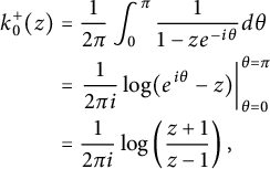 $$ \begin{align*} k_0 ^+ (z) & = \frac{1}{2\pi} \int _0 ^\pi \frac{1}{1-z e^{-i \theta}} d\theta \\ & = \left. \frac{1}{2\pi i} \log (e ^{i\theta} -z ) \right| _{\theta =0} ^{\theta = \pi} \\ & = \frac{1}{2\pi i} \log \left( \frac{z+1}{z-1} \right), \end{align*} $$
where $\log $
is the branch of the logarithm fixed by the choice of the argument function taking values in
$\log $
is the branch of the logarithm fixed by the choice of the argument function taking values in $[0, 2\pi )$
. Here, the branch cut is along the positive real axis, and
$[0, 2\pi )$
. Here, the branch cut is along the positive real axis, and
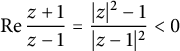 $$ \begin{align*}\mathrm{Re} \, \frac{z+1}{z-1} = \frac{|z| ^2 -1}{|z-1| ^2} <0\end{align*} $$
is strictly negative for any $z \in \mathbb {D}$
so that this formula defines a holomorphic function in
$z \in \mathbb {D}$
so that this formula defines a holomorphic function in $\mathbb {D}$
. (We know, of course, that
$\mathbb {D}$
. (We know, of course, that $k_0 ^+$
must be holomorphic in
$k_0 ^+$
must be holomorphic in $\mathbb {D}$
.) Since
$\mathbb {D}$
.) Since
 $$ \begin{align*}1 = k_0 (z) = k(z, 0) = k^+ (z , 0) + k^- (z,0) = k^+ _0 (z) + k^- _0 (z),\end{align*} $$
it follows that
 $$ \begin{align} k_0 ^- (z) = 1 - k_0 ^+ (z) = 1 - \frac{1}{2\pi i} \log \left( \frac{z+1}{z-1} \right). \end{align} $$
Also note that
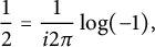 $$ \begin{align*}\frac{1}{2} = \frac{1}{i2\pi} \log (-1),\end{align*} $$
so that $\frac {1}{2} = k_0 ^+ (0) = k_0 ^- (0)$
.
$\frac {1}{2} = k_0 ^+ (0) = k_0 ^- (0)$
.
Since $V_\pm ^*$
act as backward shifts on power series, it follows that
$V_\pm ^*$
act as backward shifts on power series, it follows that $V_+ ^* k_0 ^+ = -V_- ^* k_0 ^-$
, so that
$V_+ ^* k_0 ^+ = -V_- ^* k_0 ^-$
, so that
 $$ \begin{align*}(V_+ \oplus V_-) ^* k_0 ^+ \oplus k_0 ^- \in \mathrm{Ran} \, U_\wedge = \bigvee _{h \in \mathrm{int} ( m_+ , m_- )} h \oplus -h,\end{align*} $$
as required.
5.1 Lebesgue decomposition of measures and their forms
As described in Remark 4.9 and Section 2.3, if $\mu , \lambda \geq 0$
are positive, finite, and regular Borel measures on the unit circle,
$\mu , \lambda \geq 0$
are positive, finite, and regular Borel measures on the unit circle, $\partial \mathbb {D}$
, then one can construct the Lebesgue decomposition of
$\partial \mathbb {D}$
, then one can construct the Lebesgue decomposition of $\mu $
with respect to
$\mu $
with respect to $\lambda $
by considering the densely-defined positive quadratic form,
$\lambda $
by considering the densely-defined positive quadratic form, $\mathfrak {q}_\mu : \mathscr {C} (\partial \mathbb {D} ) \times \mathscr {C} (\partial \mathbb {D}) \rightarrow 0$
, with dense form domain
$\mathfrak {q}_\mu : \mathscr {C} (\partial \mathbb {D} ) \times \mathscr {C} (\partial \mathbb {D}) \rightarrow 0$
, with dense form domain $\mathscr {C} (\partial \mathbb {D} ) \subseteq L^2 (\lambda )$
, the continuous functions on the unit circle. Namely, applying the Simon–Lebesgue decomposition to
$\mathscr {C} (\partial \mathbb {D} ) \subseteq L^2 (\lambda )$
, the continuous functions on the unit circle. Namely, applying the Simon–Lebesgue decomposition to $\mathfrak {q}_\mu $
, viewed as a positive, densely-defined form in
$\mathfrak {q}_\mu $
, viewed as a positive, densely-defined form in $L^2 (\lambda )$
, one obtains,
$L^2 (\lambda )$
, one obtains,
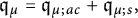 $$ \begin{align*}\mathfrak{q}_\mu = \mathfrak{q}_{\mu; ac} + \mathfrak{q} _{\mu ;s},\end{align*} $$
where $\mathfrak {q}_{\mu ;ac}$
is an absolutely continuous (closeable) form and
$\mathfrak {q}_{\mu ;ac}$
is an absolutely continuous (closeable) form and $\mathfrak {q}_s$
is a singular form and moreover,
$\mathfrak {q}_s$
is a singular form and moreover, $\mathfrak {q}_{\mu; ac} = \mathfrak {q}_{\mu _{ac}}, \mathfrak {q}_s = \mathfrak {q}_{\mu _s}$
, where
$\mathfrak {q}_{\mu; ac} = \mathfrak {q}_{\mu _{ac}}, \mathfrak {q}_s = \mathfrak {q}_{\mu _s}$
, where $\mu = \mu _{ac} + \mu _s$
is the Lebesgue decomposition.
$\mu = \mu _{ac} + \mu _s$
is the Lebesgue decomposition.
However, in this paper, since we wish to apply analytic and function theoretic methods, we instead consider the positive quadratic $Z^\lambda $
-Toeplitz form,
$Z^\lambda $
-Toeplitz form, $\mathfrak {q}_\mu $
, associated with
$\mathfrak {q}_\mu $
, associated with $\mu \geq 0$
, with dense form domain
$\mu \geq 0$
, with dense form domain $\mathrm {Dom} \, \mathfrak {q} _\mu = \mathbb {C} [\zeta ]$
or
$\mathrm {Dom} \, \mathfrak {q} _\mu = \mathbb {C} [\zeta ]$
or $\mathrm {Dom} \, \mathfrak {q}_\mu = A (\mathbb {D} )$
, in
$\mathrm {Dom} \, \mathfrak {q}_\mu = A (\mathbb {D} )$
, in $H^2 (\lambda ) \subseteq L^2 (\lambda )$
. As we will show, if
$H^2 (\lambda ) \subseteq L^2 (\lambda )$
. As we will show, if $\mathfrak {q} _\mu = \mathfrak {q}_{ac} + \mathfrak {q}_{s}$
is the Simon–Lebesgue form decomposition of
$\mathfrak {q} _\mu = \mathfrak {q}_{ac} + \mathfrak {q}_{s}$
is the Simon–Lebesgue form decomposition of $\mathfrak {q}_\mu $
in
$\mathfrak {q}_\mu $
in $H^2 (\lambda )$
, then one can define RKHSs of
$H^2 (\lambda )$
, then one can define RKHSs of $\mathfrak {q}_{ac}$
and
$\mathfrak {q}_{ac}$
and $\mathfrak {q}_s$
-Cauchy transforms,
$\mathfrak {q}_s$
-Cauchy transforms, $\mathscr {H} ^+ (\mathfrak {q}_{ac})$
and
$\mathscr {H} ^+ (\mathfrak {q}_{ac})$
and $\mathscr {H} ^+ (\mathfrak {q}_s)$
. The goal of this subsection is to compare the Lebesgue decomposition of
$\mathscr {H} ^+ (\mathfrak {q}_s)$
. The goal of this subsection is to compare the Lebesgue decomposition of $\mu $
with respect to
$\mu $
with respect to $\lambda $
with the Simon–Lebesgue decomposition of
$\lambda $
with the Simon–Lebesgue decomposition of $\mathfrak {q}_\mu $
in
$\mathfrak {q}_\mu $
in $H^2 (\lambda )$
.
$H^2 (\lambda )$
.
Let $\mu , \lambda \geq 0$
be finite and regular Borel measures on
$\mu , \lambda \geq 0$
be finite and regular Borel measures on $\partial \mathbb {D}$
. Consider the positive quadratic form,
$\partial \mathbb {D}$
. Consider the positive quadratic form, $\mathfrak {q}_\mu $
, with dense form domain,
$\mathfrak {q}_\mu $
, with dense form domain, $A (\mathbb {D} ) \subseteq H^2 (\lambda )$
. Observe that
$A (\mathbb {D} ) \subseteq H^2 (\lambda )$
. Observe that $\hat {\mathcal {H}} (\mathfrak {q}_\mu ) = H^2 (\mu + \lambda )$
so that
$\hat {\mathcal {H}} (\mathfrak {q}_\mu ) = H^2 (\mu + \lambda )$
so that $\mathbb {C} [\zeta ]$
and
$\mathbb {C} [\zeta ]$
and $\mathscr {K} _{\mathbb {D}}$
are both dense sets in this space. Consider the Simon–Lebesgue decomposition,
$\mathscr {K} _{\mathbb {D}}$
are both dense sets in this space. Consider the Simon–Lebesgue decomposition, $\mathfrak {q}_\mu = \mathfrak {q}_{ac} + \mathfrak {q}_s$
, of
$\mathfrak {q}_\mu = \mathfrak {q}_{ac} + \mathfrak {q}_s$
, of $\mathfrak {q}_\mu $
in
$\mathfrak {q}_\mu $
in $H^2 (\lambda )$
. By Theorem 4.8,
$H^2 (\lambda )$
. By Theorem 4.8, $\mathfrak {q}_{ac} \geq 0$
, is the largest closeable quadratic form bounded above by
$\mathfrak {q}_{ac} \geq 0$
, is the largest closeable quadratic form bounded above by $\mathfrak {q}_\mu $
. Since
$\mathfrak {q}_\mu $
. Since $\mathfrak {q}_{ac} \leq \mathfrak {q}_\mu $
, this implies that
$\mathfrak {q}_{ac} \leq \mathfrak {q}_\mu $
, this implies that $\mathrm {Dom} \, \mathfrak {q}_\mu = A (\mathbb {D} ) \subseteq \mathrm {Dom} \, \mathfrak {q}_{ac}$
, and if
$\mathrm {Dom} \, \mathfrak {q}_\mu = A (\mathbb {D} ) \subseteq \mathrm {Dom} \, \mathfrak {q}_{ac}$
, and if $\mathfrak {q}_D = \overline {\mathfrak {q}_{ac}}$
denotes the closure of
$\mathfrak {q}_D = \overline {\mathfrak {q}_{ac}}$
denotes the closure of $\mathfrak {q}_{ac}$
, then
$\mathfrak {q}_{ac}$
, then $A (\mathbb {D} )$
must be a form-core for the closed form
$A (\mathbb {D} )$
must be a form-core for the closed form $\mathfrak {q}_D$
by the maximality statement in Theorem 4.8. We define
$\mathfrak {q}_D$
by the maximality statement in Theorem 4.8. We define $H^2 (\mathfrak {q}_{ac} ), H^2 ( \mathfrak {q}_s )$
as the Hilbert space completion of the disk algebra,
$H^2 (\mathfrak {q}_{ac} ), H^2 ( \mathfrak {q}_s )$
as the Hilbert space completion of the disk algebra, $A (\mathbb {D})$
, modulo vectors of zero length, with respect to the pre-inner products,
$A (\mathbb {D})$
, modulo vectors of zero length, with respect to the pre-inner products, $\mathfrak {q}_{ac}, \mathfrak {q}_s$
, respectively. Since
$\mathfrak {q}_{ac}, \mathfrak {q}_s$
, respectively. Since $0 \leq \mathfrak {q}_{ac}, \mathfrak {q}_s \leq \mathfrak {q}_\mu $
, we can define the contractive co-embeddings
$0 \leq \mathfrak {q}_{ac}, \mathfrak {q}_s \leq \mathfrak {q}_\mu $
, we can define the contractive co-embeddings $E_{ac} : H^2 (\mu ) \hookrightarrow H^2 ( \mathfrak {q}_{ac}) $
and
$E_{ac} : H^2 (\mu ) \hookrightarrow H^2 ( \mathfrak {q}_{ac}) $
and $E_s : H^2 (\mu ) \hookrightarrow H^2 (\mathfrak {q}_s)$
by
$E_s : H^2 (\mu ) \hookrightarrow H^2 (\mathfrak {q}_s)$
by $E_{ac} a = a \in H^2 (\mathfrak {q}_{ac} )$
and
$E_{ac} a = a \in H^2 (\mathfrak {q}_{ac} )$
and $E_s a = a \in H^2 (\mu _s)$
. (Here, an element
$E_s a = a \in H^2 (\mu _s)$
. (Here, an element $a \in A (\mathbb {D} )$
could be equal to
$a \in A (\mathbb {D} )$
could be equal to $0$
as an element of
$0$
as an element of $H^2 (\mu )$
, or as an element of the spaces
$H^2 (\mu )$
, or as an element of the spaces $H^2 (\mathfrak {q}_{ac}), H^2 (\mathfrak {q}_s )$
. However, the inequality
$H^2 (\mathfrak {q}_{ac}), H^2 (\mathfrak {q}_s )$
. However, the inequality $0 \leq \mathfrak {q}_{ac} ,\mathfrak {q}_s \leq \mathfrak {q}_\mu $
, ensures that if
$0 \leq \mathfrak {q}_{ac} ,\mathfrak {q}_s \leq \mathfrak {q}_\mu $
, ensures that if $a \in A (\mathbb {D})$
is zero as an element of
$a \in A (\mathbb {D})$
is zero as an element of $H^2 (\mu )$
, i.e., it vanishes
$H^2 (\mu )$
, i.e., it vanishes $\mu -a.e.$
, then
$\mu -a.e.$
, then $a =0$
as element of both
$a =0$
as element of both $H^2 (\mathfrak {q}_{ac} )$
and
$H^2 (\mathfrak {q}_{ac} )$
and $H^2 (\mathfrak {q}_s)$
. A more precise notation would be to let
$H^2 (\mathfrak {q}_s)$
. A more precise notation would be to let $N_{ac}$
denote the subspace of all elements of
$N_{ac}$
denote the subspace of all elements of $A (\mathbb {D})$
of zero-length with respect to the
$A (\mathbb {D})$
of zero-length with respect to the $\mathfrak {q}_{ac}$
-pre-inner product so that equivalence classes of the form
$\mathfrak {q}_{ac}$
-pre-inner product so that equivalence classes of the form $a + N_{ac}$
,
$a + N_{ac}$
, $a \in A (\mathbb {D} )$
, are dense in
$a \in A (\mathbb {D} )$
, are dense in $H^2 (\mathfrak {q}_{ac} )$
. )
$H^2 (\mathfrak {q}_{ac} )$
. )
Observe that if $\mathscr {D} \subseteq A (\mathbb {D} )$
is any supremum-norm dense set, such as
$\mathscr {D} \subseteq A (\mathbb {D} )$
is any supremum-norm dense set, such as $\mathscr {K} _{\mathbb {D}} = \bigvee k_z$
or
$\mathscr {K} _{\mathbb {D}} = \bigvee k_z$
or $\mathbb {C} [\zeta ]$
, then
$\mathbb {C} [\zeta ]$
, then $\mathscr {D}$
is dense in
$\mathscr {D}$
is dense in $H^2 ( \mu )$
, and since the co-embedding
$H^2 ( \mu )$
, and since the co-embedding $E_{ac} : H^2 (\mu ) \hookrightarrow H^2 (\mathfrak {q}_{ac})$
is a contraction with dense range,
$E_{ac} : H^2 (\mu ) \hookrightarrow H^2 (\mathfrak {q}_{ac})$
is a contraction with dense range, $\mathscr {D}$
will be dense in
$\mathscr {D}$
will be dense in $H^2 (\mathfrak {q}_{ac})$
and it will be similarly dense in
$H^2 (\mathfrak {q}_{ac})$
and it will be similarly dense in $H^2 (\mathfrak {q}_s)$
.
$H^2 (\mathfrak {q}_s)$
.
Lemma 5.10 If $\mathfrak {q}_D = \overline {\mathfrak {q}_{ac}}$
is the closure of
$\mathfrak {q}_D = \overline {\mathfrak {q}_{ac}}$
is the closure of $\mathfrak {q}_{ac}$
, and
$\mathfrak {q}_{ac}$
, and $\mathscr {D} \subseteq A (\mathbb {D} )$
is supremum-norm dense, then
$\mathscr {D} \subseteq A (\mathbb {D} )$
is supremum-norm dense, then $\mathscr {D}$
is a core for
$\mathscr {D}$
is a core for $\sqrt {D}$
.
$\sqrt {D}$
.
Proof Since $\mathrm {Dom} \, \mathfrak {q}_\mu = A (\mathbb {D} )$
, and
$\mathrm {Dom} \, \mathfrak {q}_\mu = A (\mathbb {D} )$
, and $\mathfrak {q}_{ac} \leq \mathfrak {q}_\mu $
is the largest closeable and positive semi-definite quadratic form,
$\mathfrak {q}_{ac} \leq \mathfrak {q}_\mu $
is the largest closeable and positive semi-definite quadratic form, $A (\mathbb {D})$
is a form-core for
$A (\mathbb {D})$
is a form-core for $\mathfrak {q}_D$
, and hence a core for
$\mathfrak {q}_D$
, and hence a core for $\sqrt {D}$
. Hence,
$\sqrt {D}$
. Hence, $A (\mathbb {D} )$
is dense in
$A (\mathbb {D} )$
is dense in $\hat {\mathcal {H}} (\mathfrak {q}_D) = \hat {\mathcal {H}} (\mathfrak {q}_{ac} )$
. Given any
$\hat {\mathcal {H}} (\mathfrak {q}_D) = \hat {\mathcal {H}} (\mathfrak {q}_{ac} )$
. Given any $a \in A (\mathbb {D})$
, let
$a \in A (\mathbb {D})$
, let $x_n \in \mathscr {D}$
be a sequence which converges to a in supremum-norm. Then
$x_n \in \mathscr {D}$
be a sequence which converges to a in supremum-norm. Then
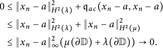 $$ \begin{align*} 0 & \leq \| x_n - a \| ^2 _{H^2 (\lambda )} + \mathfrak{q}_{ac} (x_n -a , x_n -a ) \\ & \leq \| x_n -a \| ^2 _{H^2 (\lambda )} + \| x_n - a \| ^2 _{H^2 (\mu )} \\ & \leq \| x_n -a \| ^2 _{\infty} (\mu (\partial \mathbb{D}) + \lambda (\partial \mathbb{D} ) ) \rightarrow 0. \end{align*} $$
This proves that $\mathscr {D}$
is dense in the dense subspace
$\mathscr {D}$
is dense in the dense subspace $A (\mathbb {D} ) \subseteq \hat {\mathcal {H}} (\mathfrak {q}_D)$
, and hence
$A (\mathbb {D} ) \subseteq \hat {\mathcal {H}} (\mathfrak {q}_D)$
, and hence $\mathscr {D}$
is a form-core for
$\mathscr {D}$
is a form-core for $q_D$
and a core for
$q_D$
and a core for $\sqrt {D}$
.
$\sqrt {D}$
.
Given any $h \in H^2 (\mathfrak {q}_{ac} )$
or in
$h \in H^2 (\mathfrak {q}_{ac} )$
or in $H^2 (\mathfrak {q}_s)$
, we can now define the
$H^2 (\mathfrak {q}_s)$
, we can now define the $\mathfrak {q}_{ac}$
or
$\mathfrak {q}_{ac}$
or $\mathfrak {q}_s$
-Cauchy transform of h as before:
$\mathfrak {q}_s$
-Cauchy transform of h as before:
 $$ \begin{align*}(\mathscr{C} _{ac} h ) (z) := \mathfrak{q}_{ac} ( k_z , h ),\end{align*} $$
and similarly for $\mathfrak {q}_s$
. As in Lemmas 3.1 and 3.2, Cauchy transforms of elements of
$\mathfrak {q}_s$
. As in Lemmas 3.1 and 3.2, Cauchy transforms of elements of $H^2 (\mathfrak {q}_{ac}) , H^2 (\mathfrak {q}_s)$
are holomorphic in the unit disk, and if we equip the vector space of
$H^2 (\mathfrak {q}_{ac}) , H^2 (\mathfrak {q}_s)$
are holomorphic in the unit disk, and if we equip the vector space of $\mathfrak {q}_{ac}$
-Cauchy transforms with the inner product
$\mathfrak {q}_{ac}$
-Cauchy transforms with the inner product
 $$ \begin{align*}\left\langle { \mathscr{C} _{ac} x} , {\mathscr{C} _{ac} y} \right\rangle_{ac} := \mathfrak{q}_{ac} (x,y), \end{align*} $$
we obtain a RKHS of analytic functions in the disk, $\mathscr {H} ^+ (\mathfrak {q} _{ac} )$
with reproducing kernel:
$\mathscr {H} ^+ (\mathfrak {q} _{ac} )$
with reproducing kernel:
 $$ \begin{align*}k^{(ac)} (z,w) := \mathfrak{q}_{ac} (k_z , k_w).\end{align*} $$
Finally, since $\mathfrak {q}_\mu = \mathfrak {q}_{ac} + \mathfrak {q}_s$
,
$\mathfrak {q}_\mu = \mathfrak {q}_{ac} + \mathfrak {q}_s$
, $\mathfrak {q}_\mu \geq \mathfrak {q}_{ac}, \mathfrak {q}_s \geq 0$
, we obtain the following.
$\mathfrak {q}_\mu \geq \mathfrak {q}_{ac}, \mathfrak {q}_s \geq 0$
, we obtain the following.
Proposition 5.11 The RKHS of $\mathfrak {q}_{ac}$
and
$\mathfrak {q}_{ac}$
and $\mathfrak {q}_s$
-Cauchy transforms are contractively contained in
$\mathfrak {q}_s$
-Cauchy transforms are contractively contained in $\mathscr {H} ^+ (\mu ) = \mathscr {H} ^+ (q_\mu )$
and
$\mathscr {H} ^+ (\mu ) = \mathscr {H} ^+ (q_\mu )$
and $k^\mu = k^{(ac)} + k ^s$
so that
$k^\mu = k^{(ac)} + k ^s$
so that
 $$ \begin{align*}\mathscr{H} ^+ (\mu ) = \mathscr{H} ^+ (\mathfrak{q}_{ac} ) + \mathscr{H} ^+ (\mathfrak{q}_s).\end{align*} $$
Moreover, if $\mathrm {e} _{ac} : \mathscr {H} ^+ (\mathfrak {q} _{ac} ) \hookrightarrow \mathscr {H} ^+ (\mu )$
and
$\mathrm {e} _{ac} : \mathscr {H} ^+ (\mathfrak {q} _{ac} ) \hookrightarrow \mathscr {H} ^+ (\mu )$
and $\mathrm {e} _s$
are the contractive embeddings, then
$\mathrm {e} _s$
are the contractive embeddings, then
 $$ \begin{align*}I_{\mathscr{H} ^+ (\mu )} = \mathrm{e} _{ac} \mathrm{e} _{ac} ^* + \mathrm{e} _s \mathrm{e} _s ^*.\end{align*} $$
Proof To check the decomposition of the identity, it suffices to calculate
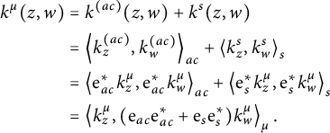 $$ \begin{align*} k ^\mu (z,w) & = k^{(ac)} (z,w) + k^s (z,w) \\ & = \left\langle {k_z ^{(ac)}} , {k_w ^{(ac)}} \right\rangle_{ac} + \left\langle {k_z ^s} , {k_w ^s} \right\rangle_s \\ & = \left\langle {\mathrm{e} _{ac} ^* k_z ^\mu} , {\mathrm{e} _{ac} ^* k ^\mu _w} \right\rangle_{ac} + \left\langle {\mathrm{e} _{s} ^* k_z ^\mu} , {\mathrm{e} _{s} ^* k ^\mu _w} \right\rangle_{s} \\ & = \left\langle {k_z ^\mu} , {(\mathrm{e}_{ac} \mathrm{e}_{ac} ^* + \mathrm{e} _s \mathrm{e} _s ^* )k_w ^\mu} \right\rangle_\mu.\\[-37pt] \end{align*} $$
Theorem 5.12 Let $\mathfrak {q}_\mu = \mathfrak {q}_{ac} + \mathfrak {q}_s$
be the Simon–Lebesgue decomposition of the form
$\mathfrak {q}_\mu = \mathfrak {q}_{ac} + \mathfrak {q}_s$
be the Simon–Lebesgue decomposition of the form $\mathfrak {q}_\mu $
with dense form domain
$\mathfrak {q}_\mu $
with dense form domain $A (\mathbb {D} )$
in
$A (\mathbb {D} )$
in $H^2 (\lambda )$
. Then,
$H^2 (\lambda )$
. Then,
 $$ \begin{align*}\mathscr{H} ^+ (\mathfrak{q}_{ac} ) = \mathrm{int} (\mu , \lambda ) ^{ -\mu } = \left( \mathscr{H} ^+ (\mu ) \cap \mathscr{H} ^+ (\lambda ) \right) ^{ -\| \cdot \| _\mu}.\end{align*} $$
If $\mathrm {e} : \mathrm {int} (\mu , \lambda ) \subseteq \mathscr {H} ^+ (\mu )\hookrightarrow \mathscr {H} ^+ (\lambda )$
is the closed embedding and
$\mathrm {e} : \mathrm {int} (\mu , \lambda ) \subseteq \mathscr {H} ^+ (\mu )\hookrightarrow \mathscr {H} ^+ (\lambda )$
is the closed embedding and $\mathfrak {q}_D = \overline {\mathfrak {q}_{ac}}$
, then
$\mathfrak {q}_D = \overline {\mathfrak {q}_{ac}}$
, then
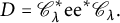 $$ \begin{align*}D = \mathscr{C} _\lambda ^* \mathrm{e} \mathrm{e} ^* \mathscr{C} _\lambda .\end{align*} $$
Lemma 5.13 Let $\mathfrak {q}_1, \mathfrak {q}_2$
be densely-defined, closed and positive semi-definite quadratic forms in a separable, complex Hilbert space,
$\mathfrak {q}_1, \mathfrak {q}_2$
be densely-defined, closed and positive semi-definite quadratic forms in a separable, complex Hilbert space, $\mathcal {H}$
. Then
$\mathcal {H}$
. Then $\mathfrak {q}_1 \leq \mathfrak {q}_2$
if and only if
$\mathfrak {q}_1 \leq \mathfrak {q}_2$
if and only if $\mathfrak {q}_1 (x,x) \leq \mathfrak {q}_2 (x,x)$
for all x in a form-core for
$\mathfrak {q}_1 (x,x) \leq \mathfrak {q}_2 (x,x)$
for all x in a form-core for $\mathfrak {q}_2$
.
$\mathfrak {q}_2$
.
Proof (of Theorem 5.12) First, since $\mathfrak {q}_{ac}$
is closeable,
$\mathfrak {q}_{ac}$
is closeable, $\overline {\mathfrak {q}}_{ac} = \mathfrak {q}_B$
for some closed, self-adjoint operator
$\overline {\mathfrak {q}}_{ac} = \mathfrak {q}_B$
for some closed, self-adjoint operator $B \geq 0$
. By construction,
$B \geq 0$
. By construction, $A (\mathbb {D} ) \subseteq \mathrm {Dom} \, \sqrt {B}$
, and
$A (\mathbb {D} ) \subseteq \mathrm {Dom} \, \sqrt {B}$
, and $\mathbb {C} [ \zeta ]$
,
$\mathbb {C} [ \zeta ]$
, $\mathscr {K} _{\mathbb {D}} = \bigvee k_z$
and
$\mathscr {K} _{\mathbb {D}} = \bigvee k_z$
and $A (\mathbb {D} )$
are all cores for
$A (\mathbb {D} )$
are all cores for $\sqrt {B}$
. Since
$\sqrt {B}$
. Since $B \geq 0$
is closed,
$B \geq 0$
is closed, $\mathrm {Dom} \, B$
is also a core for
$\mathrm {Dom} \, B$
is also a core for $\sqrt {B}$
. It follows that we can identify
$\sqrt {B}$
. It follows that we can identify $\mathrm {Dom} \, B$
with a dense subspace of
$\mathrm {Dom} \, B$
with a dense subspace of $H^2 (\mathfrak {q} _{ac} )$
. Namely, if
$H^2 (\mathfrak {q} _{ac} )$
. Namely, if $x \in \mathrm {Dom} \, B \subseteq H^2 ( \lambda )$
, we can find
$x \in \mathrm {Dom} \, B \subseteq H^2 ( \lambda )$
, we can find $a_n \in A (\mathbb {D} )$
so that
$a_n \in A (\mathbb {D} )$
so that $a_n \rightarrow x$
in
$a_n \rightarrow x$
in $H^2 (\lambda )$
and
$H^2 (\lambda )$
and $\sqrt {B} a_n \rightarrow \sqrt {B} x$
. Since
$\sqrt {B} a_n \rightarrow \sqrt {B} x$
. Since $\overline {\mathfrak {q}_{ac}} = \mathfrak {q} _B$
, it follows that
$\overline {\mathfrak {q}_{ac}} = \mathfrak {q} _B$
, it follows that $(a_n)$
is a Cauchy sequence in
$(a_n)$
is a Cauchy sequence in $H^2 (\mathfrak {q} _{ac} )$
, and we can identify
$H^2 (\mathfrak {q} _{ac} )$
, and we can identify $x \in \mathrm {Dom} \, B$
with the limit,
$x \in \mathrm {Dom} \, B$
with the limit, $\hat {x}$
, of this Cauchy sequence in the Hilbert space
$\hat {x}$
, of this Cauchy sequence in the Hilbert space $H^2 (\mathfrak {q} _{ac} )$
. Finally, since
$H^2 (\mathfrak {q} _{ac} )$
. Finally, since $\mathrm {Dom} \, B$
is a core for
$\mathrm {Dom} \, B$
is a core for $\sqrt {B}$
, for any
$\sqrt {B}$
, for any $a \in A (\mathbb {D} ) \subseteq \mathrm {Dom} \, \sqrt {B}$
, we can find
$a \in A (\mathbb {D} ) \subseteq \mathrm {Dom} \, \sqrt {B}$
, we can find $x_n \in \mathrm {Dom} \, B$
so that
$x_n \in \mathrm {Dom} \, B$
so that $x_n \rightarrow a$
and
$x_n \rightarrow a$
and $\sqrt {B} x_n \rightarrow \sqrt {B} a$
and it follows that
$\sqrt {B} x_n \rightarrow \sqrt {B} a$
and it follows that $\hat {x} _n \rightarrow a$
in
$\hat {x} _n \rightarrow a$
in $H^2 (\mathfrak {q} _{ac} )$
, so that
$H^2 (\mathfrak {q} _{ac} )$
, so that $\mathrm {Dom} \, B$
can be identified with a dense subspace of
$\mathrm {Dom} \, B$
can be identified with a dense subspace of $H^2 (\mathfrak {q} _{ac} )$
.
$H^2 (\mathfrak {q} _{ac} )$
.
Furthermore, we can then define the $\mathfrak {q}_{ac}$
-Cauchy transform of any
$\mathfrak {q}_{ac}$
-Cauchy transform of any $x \in \mathrm {Dom} \, B$
,
$x \in \mathrm {Dom} \, B$
,
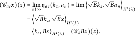 $$ \begin{align*} (\mathscr{C} _{ac} x ) (z) & = \lim _{n \uparrow \infty} \mathfrak{q}_{ac} (k_z , a_n) = \lim \left\langle {\sqrt{B} k_z} , {\sqrt{B} a_n } \right\rangle_{H^2 (\lambda )} \\ & = \left\langle {\sqrt{B} k_z} , {\sqrt{B} x} \right\rangle_{H^2 (\lambda )} \\ & = \left\langle {k_z} , {Bx} \right\rangle_{H^2 (\lambda )} = (\mathscr{C} _\lambda Bx) (z). \end{align*} $$
This proves that $\mathscr {C} _{ac} x \in \mathscr {H} ^+ (\lambda )$
. Since
$\mathscr {C} _{ac} x \in \mathscr {H} ^+ (\lambda )$
. Since $\mathscr {C} _{ac} x \in \mathscr {H} ^+ (\mathfrak {q}_{ac} ) \subseteq \mathscr {H} ^+ (\mu )$
, it follows that
$\mathscr {C} _{ac} x \in \mathscr {H} ^+ (\mathfrak {q}_{ac} ) \subseteq \mathscr {H} ^+ (\mu )$
, it follows that $\mathscr {C} _{ac} \mathrm {Dom} \, B \subseteq \mathrm {int} (\mu , \lambda )$
. Moreover, since
$\mathscr {C} _{ac} \mathrm {Dom} \, B \subseteq \mathrm {int} (\mu , \lambda )$
. Moreover, since $\mathrm {Dom} \, B$
can be identified with a dense subspace of
$\mathrm {Dom} \, B$
can be identified with a dense subspace of $H^2 (\mathfrak {q}_{ac} )$
, it follows that
$H^2 (\mathfrak {q}_{ac} )$
, it follows that $\mathscr {C} _{ac} \mathrm {Dom} \, B \subseteq \mathscr {H} ^+ (\mathfrak {q}_{ac} ) \cap \mathscr {H} ^+ (\lambda ) \subseteq \mathrm {int} (\mu ,\lambda )$
is dense in
$\mathscr {C} _{ac} \mathrm {Dom} \, B \subseteq \mathscr {H} ^+ (\mathfrak {q}_{ac} ) \cap \mathscr {H} ^+ (\lambda ) \subseteq \mathrm {int} (\mu ,\lambda )$
is dense in $\mathscr {H} ^+ (\mathfrak {q}_{ac} )$
.
$\mathscr {H} ^+ (\mathfrak {q}_{ac} )$
.
Now consider $\mathfrak {q}_D$
, where
$\mathfrak {q}_D$
, where $D = \mathscr {C} _\lambda ^* \mathrm {e} \mathrm {e} ^* \mathscr {C} _\lambda $
and
$D = \mathscr {C} _\lambda ^* \mathrm {e} \mathrm {e} ^* \mathscr {C} _\lambda $
and $\mathrm {e} : \mathrm {int} (\mu , \lambda ) \subseteq \mathscr {H} ^+ (\mu ) \hookrightarrow \mathscr {H} ^+ (\lambda )$
, as in the theorem statement. By construction,
$\mathrm {e} : \mathrm {int} (\mu , \lambda ) \subseteq \mathscr {H} ^+ (\mu ) \hookrightarrow \mathscr {H} ^+ (\lambda )$
, as in the theorem statement. By construction, $\mathscr {K} _{\mathbb {D}}$
is a core for
$\mathscr {K} _{\mathbb {D}}$
is a core for $\sqrt {D}$
, and it is also a core for B, so that this set is a form-core for both
$\sqrt {D}$
, and it is also a core for B, so that this set is a form-core for both $\mathfrak {q}_B = \overline {\mathfrak {q}_{ac}}$
and
$\mathfrak {q}_B = \overline {\mathfrak {q}_{ac}}$
and $\mathfrak {q}_D$
. It follows that
$\mathfrak {q}_D$
. It follows that $\mathfrak {q}_D | _{\mathscr {K} _{\mathbb {D}}} \leq \mathfrak {q}_\mu | _{\mathscr {K} _{\mathbb {D}}}$
is a positive closeable form so that by maximality and Lemma 5.13,
$\mathfrak {q}_D | _{\mathscr {K} _{\mathbb {D}}} \leq \mathfrak {q}_\mu | _{\mathscr {K} _{\mathbb {D}}}$
is a positive closeable form so that by maximality and Lemma 5.13, $\mathfrak {q}_D \leq \mathfrak {q}_B$
in the form-sense. Also, by construction,
$\mathfrak {q}_D \leq \mathfrak {q}_B$
in the form-sense. Also, by construction, $\mathrm {e} ^* k^\lambda _z = k ^{\mu \cap \lambda } _z$
, where
$\mathrm {e} ^* k^\lambda _z = k ^{\mu \cap \lambda } _z$
, where $k^{\mu \cap \lambda }$
is the reproducing kernel for the closed subspace
$k^{\mu \cap \lambda }$
is the reproducing kernel for the closed subspace $\mathrm {int} (\mu , \lambda ) ^{-\mu } \subseteq \mathscr {H} ^+ (\mu )$
. Hence, for any finite subset,
$\mathrm {int} (\mu , \lambda ) ^{-\mu } \subseteq \mathscr {H} ^+ (\mu )$
. Hence, for any finite subset, $\{ z_1, \dots , z_n \} \subseteq \mathbb {D}$
, if we consider any finite linear combination of Szegö kernels,
$\{ z_1, \dots , z_n \} \subseteq \mathbb {D}$
, if we consider any finite linear combination of Szegö kernels,
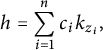 $$ \begin{align*}h = \sum _{i=1} ^n c_i k _{z_i},\end{align*} $$
then
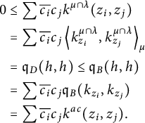 $$ \begin{align*} 0 & \leq \sum \overline{c_i} c_j k^{\mu \cap \lambda } (z_i , z_j ) \\ & = \sum \overline{c_i} c_j \left\langle {k ^{\mu \cap \lambda } _{z_i} } , {k^{\mu \cap \lambda } _{z_j}} \right\rangle_\mu \\ & = \mathfrak{q} _D (h , h) \leq \mathfrak{q} _B (h, h) \\ & = \sum \overline{c_i} c_j \mathfrak{q} _B (k_{z_i} , k_{z_j} ) \\ & = \sum \overline{c_i} c_j k^{ac} (z_i , z_j ). \end{align*} $$
That is,
 $$ \begin{align*}0 \leq [k ^{\mu \cap \lambda } (z_i ,z_j) ] _{1\leq i,j \leq n} = [\mathfrak{q}_D (k_{z_i} ,k_{z_j}) ] \leq [ \mathfrak{q}_B (k_{z_i} , k_{z_j}) ] = [k ^{ac} (z_i,z_j)],\end{align*} $$
so that $k^{\mu \cap \lambda } \leq k^{ac}$
, and by Aronszajn’s inclusion theorem,
$k^{\mu \cap \lambda } \leq k^{ac}$
, and by Aronszajn’s inclusion theorem, $\mathrm {int} (\mu , \lambda ) ^{-\mu }$
is contractively contained in
$\mathrm {int} (\mu , \lambda ) ^{-\mu }$
is contractively contained in $\mathscr {H} ^+ (\mathfrak {q}_{ac} )$
which is in turn contractively contained in
$\mathscr {H} ^+ (\mathfrak {q}_{ac} )$
which is in turn contractively contained in $\mathscr {H} ^+ (\mu )$
. Hence, if
$\mathscr {H} ^+ (\mu )$
. Hence, if $\mathrm {e} _1$
is the first embedding into
$\mathrm {e} _1$
is the first embedding into $\mathscr {H} ^+ (\mathfrak {q}_{ac} )$
and
$\mathscr {H} ^+ (\mathfrak {q}_{ac} )$
and $\mathrm {e} _2$
is the second embedding into
$\mathrm {e} _2$
is the second embedding into $\mathscr {H} ^+ (\mu )$
, the composite embedding,
$\mathscr {H} ^+ (\mu )$
, the composite embedding, $\mathrm {e} = \mathrm {e} _2 \mathrm {e} _1 : \mathrm {int} (\mu ,\lambda ) ^{-\mu } \hookrightarrow \mathscr {H} ^+ (\mu )$
is again a contractive embedding and it must be isometric since
$\mathrm {e} = \mathrm {e} _2 \mathrm {e} _1 : \mathrm {int} (\mu ,\lambda ) ^{-\mu } \hookrightarrow \mathscr {H} ^+ (\mu )$
is again a contractive embedding and it must be isometric since $\mathrm {int} (\mu , \lambda ) ^{-\mu }$
is a closed subspace of
$\mathrm {int} (\mu , \lambda ) ^{-\mu }$
is a closed subspace of $\mathscr {H} ^+ (\mu )$
. It follows that
$\mathscr {H} ^+ (\mu )$
. It follows that $\mathrm {e} _1$
must be an isometric embedding. Indeed, if there is a unit vector x so that
$\mathrm {e} _1$
must be an isometric embedding. Indeed, if there is a unit vector x so that $\| \mathrm {e} _1 x \| <1$
, then
$\| \mathrm {e} _1 x \| <1$
, then
 $$ \begin{align*}1= \|x \| = \| \mathrm{e} x \| \leq \| \mathrm{e} _2 \| \| \mathrm{e} _1 x \| < 1.\end{align*} $$
Similarly, $\mathrm {e} _2$
must be isometric on the range of
$\mathrm {e} _2$
must be isometric on the range of $\mathrm {e} _1$
. On the other hand, since
$\mathrm {e} _1$
. On the other hand, since $\mathrm {int} (\mathfrak {q}_{ac}, \lambda ) := \mathscr {H} ^+ (\mathfrak {q}_{ac} ) \cap \mathscr {H} ^+ (\lambda )$
is dense in
$\mathrm {int} (\mathfrak {q}_{ac}, \lambda ) := \mathscr {H} ^+ (\mathfrak {q}_{ac} ) \cap \mathscr {H} ^+ (\lambda )$
is dense in $\mathscr {H} ^+ (\mathfrak {q}_{ac})$
and
$\mathscr {H} ^+ (\mathfrak {q}_{ac})$
and $\mathscr {H} ^+ (\mathfrak {q}_{ac})$
is contractively contained in
$\mathscr {H} ^+ (\mathfrak {q}_{ac})$
is contractively contained in $\mathscr {H} ^+ (\mu )$
, we must have that
$\mathscr {H} ^+ (\mu )$
, we must have that $\mathrm {int} (\mathfrak {q}_{ac} , \lambda ) \subseteq \mathrm {int} (\mu , \lambda ) \subseteq \mathrm {Ran} \, \mathrm {e} _1$
. Hence, by the previous argument, since
$\mathrm {int} (\mathfrak {q}_{ac} , \lambda ) \subseteq \mathrm {int} (\mu , \lambda ) \subseteq \mathrm {Ran} \, \mathrm {e} _1$
. Hence, by the previous argument, since $\mathrm {int} (\mathfrak {q} _{ac} , \lambda ) \subseteq \mathrm {Ran} \, \mathrm {e} _1$
is dense in
$\mathrm {int} (\mathfrak {q} _{ac} , \lambda ) \subseteq \mathrm {Ran} \, \mathrm {e} _1$
is dense in $\mathscr {H} ^+ (\mathfrak {q} _{ac} )$
and
$\mathscr {H} ^+ (\mathfrak {q} _{ac} )$
and $\mathrm {e} _2$
is isometric on the range of
$\mathrm {e} _2$
is isometric on the range of $\mathrm {e} _1$
,
$\mathrm {e} _1$
, $\mathrm {e} _2 : \mathscr {H} ^+ (\mathfrak {q} _{ac} ) \hookrightarrow \mathscr {H} ^+ (\mu )$
is also an isometric inclusion. In conclusion,
$\mathrm {e} _2 : \mathscr {H} ^+ (\mathfrak {q} _{ac} ) \hookrightarrow \mathscr {H} ^+ (\mu )$
is also an isometric inclusion. In conclusion, $\mathrm {int} (\mu , \lambda ) ^{ -\mu }$
and
$\mathrm {int} (\mu , \lambda ) ^{ -\mu }$
and $\mathscr {H} ^+ (\mathfrak {q}_{ac})$
are both closed subspaces of
$\mathscr {H} ^+ (\mathfrak {q}_{ac})$
are both closed subspaces of $\mathscr {H} ^+ (\mu )$
,
$\mathscr {H} ^+ (\mu )$
, $\mathrm {int} (\mu , \lambda ) ^{-\mu }$
is a closed subspace of
$\mathrm {int} (\mu , \lambda ) ^{-\mu }$
is a closed subspace of $\mathscr {H} ^+ (\mathfrak {q}_{ac} )$
and
$\mathscr {H} ^+ (\mathfrak {q}_{ac} )$
and $\mathrm {int} (\mathfrak {q}_{ac}, \lambda ) \subseteq \mathrm {int} (\mu , \lambda )$
is dense in
$\mathrm {int} (\mathfrak {q}_{ac}, \lambda ) \subseteq \mathrm {int} (\mu , \lambda )$
is dense in $\mathscr {H} ^+ (\mathfrak {q}_{ac})$
so that
$\mathscr {H} ^+ (\mathfrak {q}_{ac})$
so that $\mathrm {int} (\mu , \lambda ) ^{-\mu } = \mathscr {H} ^+ (\mathfrak {q}_{ac})$
. It follows that
$\mathrm {int} (\mu , \lambda ) ^{-\mu } = \mathscr {H} ^+ (\mathfrak {q}_{ac})$
. It follows that $\mathfrak {q}_B = \mathfrak {q}_D$
on
$\mathfrak {q}_B = \mathfrak {q}_D$
on $\mathscr {K} _{\mathbb {D}}$
so that by Lemma 5.13 and the uniqueness of representation of closed forms,
$\mathscr {K} _{\mathbb {D}}$
so that by Lemma 5.13 and the uniqueness of representation of closed forms, $D=B$
.
$D=B$
.
Corollary 5.14 If $\mu , \lambda \geq 0$
are finite, positive, and regular Borel measures on
$\mu , \lambda \geq 0$
are finite, positive, and regular Borel measures on $\partial \mathbb {D}$
and
$\partial \mathbb {D}$
and $\mathfrak {q}_\mu $
is the densely-defined positive quadratic form associated with
$\mathfrak {q}_\mu $
is the densely-defined positive quadratic form associated with $\mu $
with form domain
$\mu $
with form domain $A (\mathbb {D} ) \subseteq H^2 (\lambda )$
, then the space of
$A (\mathbb {D} ) \subseteq H^2 (\lambda )$
, then the space of $\mu $
-Cauchy transforms decomposes as the orthogonal direct sum,
$\mu $
-Cauchy transforms decomposes as the orthogonal direct sum,
 $$ \begin{align*}\mathscr{H} ^+ (\mu ) = \mathscr{H} ^+ (\mathfrak{q}_{ac} ) \oplus \mathscr{H} ^+ (\mathfrak{q}_s ).\end{align*} $$
In particular, $\mathscr {H} ^+ (\mathfrak {q}_s) \cap \mathrm {int} (\mu ,\lambda ) = \{ 0 \}$
.
$\mathscr {H} ^+ (\mathfrak {q}_s) \cap \mathrm {int} (\mu ,\lambda ) = \{ 0 \}$
.
Proof By Proposition 5.11 and Theorem 4.8, we have that the identity operator on $\mathscr {H} ^+ (\mu )$
decomposes as
$\mathscr {H} ^+ (\mu )$
decomposes as
 $$ \begin{align*}I_\mu = \mathrm{e} _{ac} \mathrm{e} _{ac} ^* + \mathrm{e} _s \mathrm{e} _s ^*,\end{align*} $$
and $\mathscr {H} ^+ (\mathfrak {q}_{ac} ) = \mathrm {int} (\mu ,\lambda ) ^{-\mu }$
is a closed subspace of
$\mathscr {H} ^+ (\mathfrak {q}_{ac} ) = \mathrm {int} (\mu ,\lambda ) ^{-\mu }$
is a closed subspace of $\mathscr {H} ^+ (\mu )$
so that the contractive embedding,
$\mathscr {H} ^+ (\mu )$
so that the contractive embedding, $\mathrm {e} _{ac} : \mathscr {H} ^+ (\mathfrak {q}_{ac} ) \hookrightarrow \mathscr {H} ^+ (\mu )$
is an isometry. Hence,
$\mathrm {e} _{ac} : \mathscr {H} ^+ (\mathfrak {q}_{ac} ) \hookrightarrow \mathscr {H} ^+ (\mu )$
is an isometry. Hence, $P_{ac} := \mathrm {e} _{ac} \mathrm {e}_{ac} ^*$
is an orthogonal projection onto the range of
$P_{ac} := \mathrm {e} _{ac} \mathrm {e}_{ac} ^*$
is an orthogonal projection onto the range of $\mathrm {e} _{ac}$
and hence
$\mathrm {e} _{ac}$
and hence $P_s = I - P_{ac} = \mathrm {e} _s \mathrm {e} _s ^*$
is the projection onto the orthogonal complement of
$P_s = I - P_{ac} = \mathrm {e} _s \mathrm {e} _s ^*$
is the projection onto the orthogonal complement of $\mathrm {Ran} \, \mathrm {e} _{ac}$
in
$\mathrm {Ran} \, \mathrm {e} _{ac}$
in $\mathscr {H} ^+ (\mu )$
. It follows that
$\mathscr {H} ^+ (\mu )$
. It follows that $\mathrm {e} _s$
is also an isometric embedding and that we can identify
$\mathrm {e} _s$
is also an isometric embedding and that we can identify $\mathscr {H} ^+ (\mathfrak {q}_{ac}), \mathscr {H} ^+ (\mathfrak {q} _s)$
with the ranges of these isometric embeddings so that
$\mathscr {H} ^+ (\mathfrak {q}_{ac}), \mathscr {H} ^+ (\mathfrak {q} _s)$
with the ranges of these isometric embeddings so that
 $$ \begin{align*}\mathscr{H} ^+ (\mu ) = \mathscr{H} ^+ (\mathfrak{q}_{ac} ) \oplus \mathscr{H} ^+ (\mathfrak{q} _s ).\\[-35pt] \end{align*} $$
Corollary 5.15 Let $\mu , \lambda $
be positive, finite, and regular Borel measures on the unit circle. The Lebesgue decomposition of
$\mu , \lambda $
be positive, finite, and regular Borel measures on the unit circle. The Lebesgue decomposition of $\mu $
with respect to
$\mu $
with respect to $\lambda $
,
$\lambda $
, $\mu = \mu _{ac} + \mu _s$
, coincides with the Simon–Lebesgue decomposition of
$\mu = \mu _{ac} + \mu _s$
, coincides with the Simon–Lebesgue decomposition of $\mathfrak {q}_\mu $
with form domain
$\mathfrak {q}_\mu $
with form domain $\mathrm {Dom} \, \mathfrak {q}_\mu = A (\mathbb {D} )$
in
$\mathrm {Dom} \, \mathfrak {q}_\mu = A (\mathbb {D} )$
in $H^2 (\lambda )$
,
$H^2 (\lambda )$
, $\mathfrak {q}_\mu = \mathfrak {q}_{ac} + \mathfrak {q}_s$
, in the sense that
$\mathfrak {q}_\mu = \mathfrak {q}_{ac} + \mathfrak {q}_s$
, in the sense that $\mathfrak {q}_{ac} = \mathfrak {q}_{\mu _{ac}}$
and
$\mathfrak {q}_{ac} = \mathfrak {q}_{\mu _{ac}}$
and $\mathfrak {q}_s = \mathfrak {q}_{\mu _s}$
if and only if
$\mathfrak {q}_s = \mathfrak {q}_{\mu _s}$
if and only if $\mathrm {int} (\mu , \lambda )$
is
$\mathrm {int} (\mu , \lambda )$
is $V^\mu $
-reducing.
$V^\mu $
-reducing.
Remark 5.16 More generally, one can apply the methods of this section to construct a Lebesgue decomposition for pairs of positive kernel functions $k, K$
on the same set, X, see Appendix A.
$k, K$
on the same set, X, see Appendix A.
Example 5.17 (Lebesgue measure on the half-circles)
As before, let $m_\pm $
denote normalized Lebesgue measure restricted to the upper and lower half-circles. These are mutually singular measures so that
$m_\pm $
denote normalized Lebesgue measure restricted to the upper and lower half-circles. These are mutually singular measures so that $m_+ = m_{+; s}$
is the singular part of
$m_+ = m_{+; s}$
is the singular part of $m_+$
with respect to
$m_+$
with respect to $m_-$
, and yet by Example 5.9,
$m_-$
, and yet by Example 5.9, $\mathrm {int} (m_+ , m_-) \neq \{ 0 \}$
, so that
$\mathrm {int} (m_+ , m_-) \neq \{ 0 \}$
, so that $\mathfrak {q}_+ = \mathfrak {q}_{m_+}$
has a Simon–Lebesgue decomposition
$\mathfrak {q}_+ = \mathfrak {q}_{m_+}$
has a Simon–Lebesgue decomposition $\mathfrak {q}_+ = \mathfrak {q}_{ac} + \mathfrak {q} _s$
in
$\mathfrak {q}_+ = \mathfrak {q}_{ac} + \mathfrak {q} _s$
in $H^2 (m_-)$
, where
$H^2 (m_-)$
, where $\mathfrak {q}_{ac}$
is nontrivial, by Theorem 5.12. Moreover, in this example,
$\mathfrak {q}_{ac}$
is nontrivial, by Theorem 5.12. Moreover, in this example, $m_-$
is extreme, so that
$m_-$
is extreme, so that $H^2 (m_-) = L^2 (m_-)$
. This means that while the quadratic form,
$H^2 (m_-) = L^2 (m_-)$
. This means that while the quadratic form, $\mathfrak {q}_\mu $
, associated with
$\mathfrak {q}_\mu $
, associated with $\mu $
, with dense form domain,
$\mu $
, with dense form domain, $A (\mathbb {D} ) \subseteq L^2 (m_- ) = H^2 (m _-)$
has nonzero absolutely continuous part, if we instead define the form domain of
$A (\mathbb {D} ) \subseteq L^2 (m_- ) = H^2 (m _-)$
has nonzero absolutely continuous part, if we instead define the form domain of $\mathfrak {q}_\mu $
to be
$\mathfrak {q}_\mu $
to be $\mathrm {Dom} \, \mathfrak {q}_\mu = \mathscr {C} (\partial \mathbb {D} )$
, then, with this form domain,
$\mathrm {Dom} \, \mathfrak {q}_\mu = \mathscr {C} (\partial \mathbb {D} )$
, then, with this form domain, $\mathfrak {q}_\mu $
has vanishing absolutely continuous part (since the decompositions of
$\mathfrak {q}_\mu $
has vanishing absolutely continuous part (since the decompositions of $\mathfrak {q}_\mu $
and
$\mathfrak {q}_\mu $
and $\mu $
always coincide in this case, see Remark 4.9). This shows, that in dealing with these unbounded positive quadratic Toeplitz forms, the choice of form domain is crucial!
$\mu $
always coincide in this case, see Remark 4.9). This shows, that in dealing with these unbounded positive quadratic Toeplitz forms, the choice of form domain is crucial!
5.2 Lebesgue decomposition for arbitrary measures
The question remains: If $\mu , \lambda \geq 0$
are arbitrary, how can we construct the Lebesgue decomposition of
$\mu , \lambda \geq 0$
are arbitrary, how can we construct the Lebesgue decomposition of $\mu $
with respect of
$\mu $
with respect of $\lambda $
using reproducing kernel theory and their spaces of Cauchy transforms? If
$\lambda $
using reproducing kernel theory and their spaces of Cauchy transforms? If $\lambda $
is non-extreme, or more generally if
$\lambda $
is non-extreme, or more generally if $\mathrm {int} (\mu , \lambda )$
is
$\mathrm {int} (\mu , \lambda )$
is $V_\mu $
-reducing, Theorem 5.5 provides a satisfying answer. However, as Proposition 5.7, Example 5.9, and Theorem 5.12 show, the intersection of the spaces of
$V_\mu $
-reducing, Theorem 5.5 provides a satisfying answer. However, as Proposition 5.7, Example 5.9, and Theorem 5.12 show, the intersection of the spaces of $\mu $
and
$\mu $
and $\lambda $
Cauchy transforms cannot be reducing in general, and that there are examples of pairs of positive measures
$\lambda $
Cauchy transforms cannot be reducing in general, and that there are examples of pairs of positive measures $\mu , \lambda $
, for which
$\mu , \lambda $
, for which $\mathrm {int} (\mu ,\lambda )$
cannot be equal to, or even contain, the space of Cauchy transforms of any nonzero positive measure.
$\mathrm {int} (\mu ,\lambda )$
cannot be equal to, or even contain, the space of Cauchy transforms of any nonzero positive measure.
By Theorem 4.12, we do know that if $\mu = \mu _{ac} + \mu _s$
is the Legbesgue decomposition of
$\mu = \mu _{ac} + \mu _s$
is the Legbesgue decomposition of $\mu $
with respect to
$\mu $
with respect to $\lambda $
, that
$\lambda $
, that $\mu _{ac} \ll _{RK} \lambda $
so that
$\mu _{ac} \ll _{RK} \lambda $
so that $\mathrm {int} (\mu _{ac} , \lambda ) \subseteq \mathrm {int} (\mu , \lambda ) \subseteq \mathrm {int} (\mu , \lambda ) ^{-\mu } = \mathscr {H} ^+ (q_{ac} )$
. The final result below provides an abstract characterization of the Lebesgue decomposition for arbitrary pairs of positive measures.
$\mathrm {int} (\mu _{ac} , \lambda ) \subseteq \mathrm {int} (\mu , \lambda ) \subseteq \mathrm {int} (\mu , \lambda ) ^{-\mu } = \mathscr {H} ^+ (q_{ac} )$
. The final result below provides an abstract characterization of the Lebesgue decomposition for arbitrary pairs of positive measures.
Theorem 5.18 If $\mu = \mu _{ac} + \mu _s$
is the Lebesgue decomposition of
$\mu = \mu _{ac} + \mu _s$
is the Lebesgue decomposition of $\mu $
with respect to
$\mu $
with respect to $\lambda $
and
$\lambda $
and $\mathfrak {q}_\mu = \mathfrak {q}_{ac} +\mathfrak {q}_s$
is the Simon–Lebesgue form decomposition of
$\mathfrak {q}_\mu = \mathfrak {q}_{ac} +\mathfrak {q}_s$
is the Simon–Lebesgue form decomposition of $\mathfrak {q}_\mu $
in
$\mathfrak {q}_\mu $
in $H^2 (\lambda ),$
then
$H^2 (\lambda ),$
then $\mathfrak {q}_{\mu _{ac}} \leq \mathfrak {q}_{ac}$
. Moreover,
$\mathfrak {q}_{\mu _{ac}} \leq \mathfrak {q}_{ac}$
. Moreover, $\mathscr {H} ^+ (\mu _{ac} )$
is the maximal RKHS,
$\mathscr {H} ^+ (\mu _{ac} )$
is the maximal RKHS, $\mathcal {H} (k)$
, in
$\mathcal {H} (k)$
, in $\mathbb {D}$
with the following property:
$\mathbb {D}$
with the following property: $\mathcal {H} (k) \cap \mathscr {H} ^+ (\lambda ) \subseteq \mathrm {int} (\mu ,\lambda )$
is dense in
$\mathcal {H} (k) \cap \mathscr {H} ^+ (\lambda ) \subseteq \mathrm {int} (\mu ,\lambda )$
is dense in $\mathcal {H} (k)$
,
$\mathcal {H} (k)$
, $\mathcal {H} (k) \subseteq \mathscr {H} ^+ (\mu )$
is contractively contained, and if
$\mathcal {H} (k) \subseteq \mathscr {H} ^+ (\mu )$
is contractively contained, and if $\mathrm {e} : \mathcal {H} (k) \hookrightarrow \mathscr {H} ^+ (\mu )$
is the contractive embedding, then
$\mathrm {e} : \mathcal {H} (k) \hookrightarrow \mathscr {H} ^+ (\mu )$
is the contractive embedding, then $\mathrm {e} \mathrm {e} ^*$
is
$\mathrm {e} \mathrm {e} ^*$
is $V_\mu $
-Toeplitz. Equivalently,
$V_\mu $
-Toeplitz. Equivalently, $q_{\mu _{ac}}$
is the largest closeable
$q_{\mu _{ac}}$
is the largest closeable $Z^\lambda $
-Toeplitz form bounded above by
$Z^\lambda $
-Toeplitz form bounded above by $q_\mu $
.
$q_\mu $
.
Moreover, if $\mathrm {e} _1 := \mathrm {e} _{\mu _{ac}}$
and
$\mathrm {e} _1 := \mathrm {e} _{\mu _{ac}}$
and $\mathrm {e} _2 = \mathrm {e} _{\mu _s}$
, then
$\mathrm {e} _2 = \mathrm {e} _{\mu _s}$
, then $I_\mu = \mathrm {e} _1 \mathrm {e} _1 ^* + \mathrm {e} _2 \mathrm {e} _2 ^*$
. Hence, we can identify
$I_\mu = \mathrm {e} _1 \mathrm {e} _1 ^* + \mathrm {e} _2 \mathrm {e} _2 ^*$
. Hence, we can identify $\mathscr {H} ^+ (\mu _{ac})$
with the operator-range space
$\mathscr {H} ^+ (\mu _{ac})$
with the operator-range space $\mathscr {R} (\mathrm {e} _1)$
and
$\mathscr {R} (\mathrm {e} _1)$
and $\mathscr {H} ^+ (\mu _s)$
with
$\mathscr {H} ^+ (\mu _s)$
with $\mathscr {R} (\mathrm {e} _2) = \mathscr {R} ^c (\mathrm {e} _1)$
, the complementary space of
$\mathscr {R} (\mathrm {e} _2) = \mathscr {R} ^c (\mathrm {e} _1)$
, the complementary space of $\mathscr {H} ^+ (\mu _{ac})$
in the sense of deBranges and Rovnyak and
$\mathscr {H} ^+ (\mu _{ac})$
in the sense of deBranges and Rovnyak and
 $$ \begin{align*}\mathscr{H} ^+ (\mu ) = \mathscr{H} ^+ (\mu _{ac} ) + \mathscr{H} ^+ (\mu _s).\end{align*} $$

Remark 5.19 In the case where the complementary space decomposition of $\mathscr {H} ^+ (\mu ) = \mathscr {H} ^+ (\mu _{ac} ) + \mathscr {H} ^+ (\mu _s )$
, appearing in the above theorem statement, is not an orthogonal direct sum, this yields a corresponding decomposition of the quadratic form
$\mathscr {H} ^+ (\mu ) = \mathscr {H} ^+ (\mu _{ac} ) + \mathscr {H} ^+ (\mu _s )$
, appearing in the above theorem statement, is not an orthogonal direct sum, this yields a corresponding decomposition of the quadratic form $\mathfrak {q} _\mu $
,
$\mathfrak {q} _\mu $
,
 $$ \begin{align} \mathfrak{q} _\mu = \mathfrak{q} _{\mu _{ac}} + \mathfrak{q} _{\mu _s}, \end{align} $$
where $\mathfrak {q} _{\mu _{ac} } < \mathfrak {q} _{ac}$
and
$\mathfrak {q} _{\mu _{ac} } < \mathfrak {q} _{ac}$
and $\mathfrak {q} _\mu = \mathfrak {q} _{ac} + \mathfrak {q} _s$
is the Simon–Lebesgue decomposition of
$\mathfrak {q} _\mu = \mathfrak {q} _{ac} + \mathfrak {q} _s$
is the Simon–Lebesgue decomposition of $\mathfrak {q} _\mu $
. In this case, the decomposition of Equation (5.3) is an example of a “pseudo-orthogonal” Lebesgue decomposition of
$\mathfrak {q} _\mu $
. In this case, the decomposition of Equation (5.3) is an example of a “pseudo-orthogonal” Lebesgue decomposition of $\mathfrak {q} _\mu $
as recently defined and studied in [Reference Hassi and de Snoo11].
$\mathfrak {q} _\mu $
as recently defined and studied in [Reference Hassi and de Snoo11].
The previous theorem is, while interesting, admittedly not very practical for construction of the Lebesgue decomposition of $\mu $
with respect to
$\mu $
with respect to $\lambda $
. A simpler, albeit somewhat ad hoc, approach using our reproducing kernel methods is simply to “add Lebesgue measure.” Namely, if
$\lambda $
. A simpler, albeit somewhat ad hoc, approach using our reproducing kernel methods is simply to “add Lebesgue measure.” Namely, if $\mu _{ac; \lambda }$
is the absolutely continuous part of
$\mu _{ac; \lambda }$
is the absolutely continuous part of $\mu $
with respect to
$\mu $
with respect to $\lambda $
, then
$\lambda $
, then $\mu _{ac; \lambda } = \mu _{ac; \lambda + m} - \mu _{ac; m}$
and both
$\mu _{ac; \lambda } = \mu _{ac; \lambda + m} - \mu _{ac; m}$
and both $\lambda + m$
and m are non-extreme so that Theorem 5.5 applies.
$\lambda + m$
and m are non-extreme so that Theorem 5.5 applies.
A Lebesgue decomposition of positive kernels
Let K be a fixed positive kernel function on a set, X. Given any other positive kernel, k, on X, we can associate with it the densely-defined and positive semi-definite quadratic form, $\mathfrak {q} _k : \mathrm {Dom} \, \mathfrak {q} _k \times \mathrm {Dom} \, \mathfrak {q} _k \rightarrow \mathbb {C}$
, with dense form domain
$\mathfrak {q} _k : \mathrm {Dom} \, \mathfrak {q} _k \times \mathrm {Dom} \, \mathfrak {q} _k \rightarrow \mathbb {C}$
, with dense form domain $\mathrm {Dom} \, \mathfrak {q} _k := \bigvee _{x \in X} K_x$
in
$\mathrm {Dom} \, \mathfrak {q} _k := \bigvee _{x \in X} K_x$
in $\mathcal {H} (K)$
,
$\mathcal {H} (K)$
,
 $$ \begin{align*}\mathfrak{q} _k (K_x , K_y ) := k(x,y).\end{align*} $$
One can then apply B. Simon’s Lebesgue decomposition of positive quadratic forms to $\mathfrak {q} _k$
. Such a Lebesgue decomposition of positive kernels was first considered in [Reference Hassi, Sebestyén and de Snoo12, Section 7, Theorem 7.2]. The theorem below provides some more details about this decomposition.
$\mathfrak {q} _k$
. Such a Lebesgue decomposition of positive kernels was first considered in [Reference Hassi, Sebestyén and de Snoo12, Section 7, Theorem 7.2]. The theorem below provides some more details about this decomposition.
Theorem A.1 Let $k,K$
be positive kernel functions on a set, X. If
$k,K$
be positive kernel functions on a set, X. If $\mathfrak {q} _k$
is the densely-defined positive quadratic form of k in
$\mathfrak {q} _k$
is the densely-defined positive quadratic form of k in $\mathcal {H} (K)$
, as defined above, with Simon–Lebesgue form decomposition
$\mathcal {H} (K)$
, as defined above, with Simon–Lebesgue form decomposition $\mathfrak {q} _{k} = \mathfrak {q} _{ac} + \mathfrak {q} _s$
, then there are positive kernels,
$\mathfrak {q} _{k} = \mathfrak {q} _{ac} + \mathfrak {q} _s$
, then there are positive kernels, $k^{ac}$
and
$k^{ac}$
and $k^s$
on X, so that
$k^s$
on X, so that $\mathfrak {q} _{ac} = \mathfrak {q} _{k^{(ac)}}$
,
$\mathfrak {q} _{ac} = \mathfrak {q} _{k^{(ac)}}$
, $\mathfrak {q} _s = \mathfrak {q} _{k^s}$
,
$\mathfrak {q} _s = \mathfrak {q} _{k^s}$
, $k = k^{ac} + k^s$
, and
$k = k^{ac} + k^s$
, and
 $$ \begin{align*}\mathcal{H} (k) = \mathcal{H} (k ^{ac} ) \oplus \mathcal{H} (k^s ).\end{align*} $$
Moreover, $\mathcal {H} (k ^{ac} ) = \mathrm {int} (k , K) ^{-k} := \left ( \mathcal {H} (k) \cap \mathcal {H} (K) \right ) ^{-\| \cdot \| _k }$
, and if
$\mathcal {H} (k ^{ac} ) = \mathrm {int} (k , K) ^{-k} := \left ( \mathcal {H} (k) \cap \mathcal {H} (K) \right ) ^{-\| \cdot \| _k }$
, and if $\mathrm {e} : \mathrm {int} (k, K) \hookrightarrow \mathcal {H} (K)$
is the (closed) embedding, then
$\mathrm {e} : \mathrm {int} (k, K) \hookrightarrow \mathcal {H} (K)$
is the (closed) embedding, then $\overline {\mathfrak {q} _{ac}} = \mathfrak {q} _{\mathrm {e}\mathrm {e} ^*}$
.
$\overline {\mathfrak {q} _{ac}} = \mathfrak {q} _{\mathrm {e}\mathrm {e} ^*}$
.
In the above, $\mathrm {int} (k,K) := \mathcal {H} (k) \cap \mathcal {H} (K)$
.
$\mathrm {int} (k,K) := \mathcal {H} (k) \cap \mathcal {H} (K)$
.
Proof Let $h := \sum _{i=1} ^n c_i K_{x_i}$
be any finite linear combination of the kernels
$h := \sum _{i=1} ^n c_i K_{x_i}$
be any finite linear combination of the kernels $K_{x_i}$
,
$K_{x_i}$
, $\{ x_i \} _{i=1} ^n \subseteq X$
. Then, since
$\{ x_i \} _{i=1} ^n \subseteq X$
. Then, since $\mathfrak {q} _{ac} \leq \mathfrak {q} _k$
, we obtain that
$\mathfrak {q} _{ac} \leq \mathfrak {q} _k$
, we obtain that
 $$ \begin{align*} \sum \overline{c_i} c_j k (x_i , x_j ) & = \sum \overline{c_i } c_j \mathfrak{q} _k (x_i , x_j ) \\ & = \mathfrak{q} _k (h , h) \geq \mathfrak{q} _{ac} (h , h) \geq 0, \end{align*} $$
where
 $$ \begin{align*}0 \leq \mathfrak{q} _{ac} (h , h) = \sum \overline{c_i} c_j \mathfrak{q} _{ac} ( K_{x_i} , K_{x_j} ).\end{align*} $$
It follows that
 $$ \begin{align*}k^{ac} (x,y) := \mathfrak{q} _{ac} (K_x , K_y),\end{align*} $$
defines a positive kernel function on X so that $0 \leq k^{ac} \leq k$
. Similarly,
$0 \leq k^{ac} \leq k$
. Similarly, $k^s (x,y) := \mathfrak {q} _s (K_x , K_y)$
defines a positive kernel function on X so that
$k^s (x,y) := \mathfrak {q} _s (K_x , K_y)$
defines a positive kernel function on X so that $0 \leq k^s \leq k$
, and since
$0 \leq k^s \leq k$
, and since $\mathfrak {q} _k = \mathfrak {q} _{ac} +\mathfrak {q} _s$
, we obtain that
$\mathfrak {q} _k = \mathfrak {q} _{ac} +\mathfrak {q} _s$
, we obtain that $k^{ac} + k^s = k$
.
$k^{ac} + k^s = k$
.
By definition, $\mathfrak {q} _{ac}$
is the largest closeable quadratic form bounded above by
$\mathfrak {q} _{ac}$
is the largest closeable quadratic form bounded above by $\mathfrak {q} _k$
. In particular,
$\mathfrak {q} _k$
. In particular, $\overline {\mathfrak {q} _{ac}} =\mathfrak {q} _D$
is the positive form of some densely-defined, self-adjoint, and positive semi-definite operator D, so that
$\overline {\mathfrak {q} _{ac}} =\mathfrak {q} _D$
is the positive form of some densely-defined, self-adjoint, and positive semi-definite operator D, so that $\mathscr {K} _x := \bigvee _{x \in X} K_x$
is a core for
$\mathscr {K} _x := \bigvee _{x \in X} K_x$
is a core for $\sqrt {D}$
. (Here,
$\sqrt {D}$
. (Here, $\bigvee $
denotes non-closed linear span.) If
$\bigvee $
denotes non-closed linear span.) If $\mathrm {e} : \mathrm {int} (k, K) \subseteq \mathrm {int} (k,K) ^{-k} \hookrightarrow \mathcal {H} (K)$
is the densely-defined and closed embedding, let
$\mathrm {e} : \mathrm {int} (k, K) \subseteq \mathrm {int} (k,K) ^{-k} \hookrightarrow \mathcal {H} (K)$
is the densely-defined and closed embedding, let $A := \mathrm {e} \mathrm {e} ^*$
. We claim that
$A := \mathrm {e} \mathrm {e} ^*$
. We claim that $A=D$
. First,
$A=D$
. First, $A \geq 0$
is self-adjoint, hence closed, and since
$A \geq 0$
is self-adjoint, hence closed, and since $\mathrm {e}$
is trivially a multiplier, we obtain that
$\mathrm {e}$
is trivially a multiplier, we obtain that
 $$ \begin{align*}\mathfrak{q} _A ( K_x , K_y ) = \left\langle {\mathrm{e} ^* K_x} , {\mathrm{e} ^* K_y} \right\rangle_k = \left\langle {k ^{\cap} _x} , {k^\cap _y} \right\rangle_k = k^\cap (x,y),\end{align*} $$
where $k^\cap $
denotes the reproducing kernel of the subspace
$k^\cap $
denotes the reproducing kernel of the subspace $\mathrm {int} (k,K) ^{-k} \subseteq \mathcal {H} (k)$
, the closure of the intersection space,
$\mathrm {int} (k,K) ^{-k} \subseteq \mathcal {H} (k)$
, the closure of the intersection space, $\mathrm {int}(k,K)$
in
$\mathrm {int}(k,K)$
in $\mathcal {H} (k)$
. In particular, since
$\mathcal {H} (k)$
. In particular, since $k^\cap _x = P _\cap k_x$
, where
$k^\cap _x = P _\cap k_x$
, where $P_\cap : \mathcal {H} (k) \rightarrow \mathrm {int} (k , K) ^{-k}$
is the orthogonal projection, it follows that
$P_\cap : \mathcal {H} (k) \rightarrow \mathrm {int} (k , K) ^{-k}$
is the orthogonal projection, it follows that $k^\cap \leq k$
, and hence that
$k^\cap \leq k$
, and hence that $\mathfrak {q} _A \leq \mathfrak {q} _k$
. Since
$\mathfrak {q} _A \leq \mathfrak {q} _k$
. Since $\mathfrak {q} _A | _{\mathscr {K} _X}$
is closeable, it follows, by maximality of the Simon–Lebesgue decomposition, that
$\mathfrak {q} _A | _{\mathscr {K} _X}$
is closeable, it follows, by maximality of the Simon–Lebesgue decomposition, that $\mathfrak {q} _A \leq \mathfrak {q} _D$
. This inequality implies that
$\mathfrak {q} _A \leq \mathfrak {q} _D$
. This inequality implies that $k^\cap \leq k^{ac}$
as positive kernels on X.
$k^\cap \leq k^{ac}$
as positive kernels on X.
Now suppose that $h \in \mathrm {Dom} \, D \subseteq \mathcal {H} (K)$
and choose
$h \in \mathrm {Dom} \, D \subseteq \mathcal {H} (K)$
and choose $h_n \in \mathscr {K} _X = \bigvee _{x \in X} K_x$
so that
$h_n \in \mathscr {K} _X = \bigvee _{x \in X} K_x$
so that $h_n \rightarrow h$
and
$h_n \rightarrow h$
and $\sqrt {D} h_n \rightarrow \sqrt {D} h$
. (This can be done since
$\sqrt {D} h_n \rightarrow \sqrt {D} h$
. (This can be done since $\mathrm {Dom} \, D$
is a core for
$\mathrm {Dom} \, D$
is a core for $\sqrt {D}$
.) If
$\sqrt {D}$
.) If $h_n = \sum _{j=1} ^{m_n} c_j (n) K_{x_j (n)}$
, a finite linear combination, then note that
$h_n = \sum _{j=1} ^{m_n} c_j (n) K_{x_j (n)}$
, a finite linear combination, then note that
 $$ \begin{align*} (Dh) (x) & = \lim _{n \uparrow \infty } \sum c_j (n) \left\langle {\sqrt{D} K_x} , {\sqrt{D} K_{x_j (n) }} \right\rangle_K \\ & = \lim \sum c_j (n) k^{ac} (x,x_j (n) ) = \lim g_n (x), \end{align*} $$
where
 $$ \begin{align*}g_n = \sum c_j (n) k^{ac} _{x_j (n) } \in \mathcal{H} ( k^{ac} ) \subseteq \mathcal{H} (k).\end{align*} $$
Moreover,
 $$ \begin{align*} \| g_n \| ^2 _{k^{ac}} & = \sum _{i,j} \overline{c_i (n) } c_j (n) k^{ac} (x_i (n) , x_j (n) ) \\ & = \left\langle {\sqrt{D} h_n} , {\sqrt{D} h_n} \right\rangle _K \rightarrow \| \sqrt{D} h \| _K ^2, \end{align*} $$
so that the sequence $(g_n ) \subseteq \mathcal {H} (k^{ac})$
is uniformly bounded in norm. Since
$(g_n ) \subseteq \mathcal {H} (k^{ac})$
is uniformly bounded in norm. Since $g_n (x) \rightarrow (Dh) (x)$
pointwise in X, this and uniform boundedness imply that
$g_n (x) \rightarrow (Dh) (x)$
pointwise in X, this and uniform boundedness imply that $g_n$
converges weakly to the function
$g_n$
converges weakly to the function $Dh$
. Since Hilbert spaces are weakly closed, the function
$Dh$
. Since Hilbert spaces are weakly closed, the function $Dh \in \mathcal {H} (k^{ac} ) \subseteq \mathcal {H} (k)$
, and also
$Dh \in \mathcal {H} (k^{ac} ) \subseteq \mathcal {H} (k)$
, and also $Dh \in \mathcal {H} (K)$
so that
$Dh \in \mathcal {H} (K)$
so that $Dh \in \mathrm {int} (k, K) \subseteq \mathcal {H} (k ^\cap )$
. Hence
$Dh \in \mathrm {int} (k, K) \subseteq \mathcal {H} (k ^\cap )$
. Hence $Dh \in \mathcal {H} (k^{ac} )$
and
$Dh \in \mathcal {H} (k^{ac} )$
and
 $$ \begin{align*}\| Dh \| ^2 _{k^{ac}} = \| \sqrt{D} h \| ^2 _K.\end{align*} $$
Let $\mathrm {j} _1 : \mathcal {H} (k^\cap ) \hookrightarrow \mathcal {H} (k^{ac})$
and
$\mathrm {j} _1 : \mathcal {H} (k^\cap ) \hookrightarrow \mathcal {H} (k^{ac})$
and $\mathrm {j} _2 : \mathcal {H} (k^{ac} ) \hookrightarrow \mathcal {H} (k)$
be the contractive embeddings. Then
$\mathrm {j} _2 : \mathcal {H} (k^{ac} ) \hookrightarrow \mathcal {H} (k)$
be the contractive embeddings. Then $\mathrm {j} := \mathrm {j} _2 \mathrm {j} _1 : \mathcal {H} (k ^\cap ) \hookrightarrow \mathcal {H} (k)$
is the isometric embedding of the subspace
$\mathrm {j} := \mathrm {j} _2 \mathrm {j} _1 : \mathcal {H} (k ^\cap ) \hookrightarrow \mathcal {H} (k)$
is the isometric embedding of the subspace $\mathcal {H} (k ^\cap ) \subseteq \mathcal {H} (k)$
into
$\mathcal {H} (k ^\cap ) \subseteq \mathcal {H} (k)$
into $\mathcal {H} (k)$
. It follows that
$\mathcal {H} (k)$
. It follows that $\mathrm {j} _1$
must be isometric and
$\mathrm {j} _1$
must be isometric and $\mathrm {j} _2$
must be isometric on the range of
$\mathrm {j} _2$
must be isometric on the range of $\mathrm {j} _1$
in
$\mathrm {j} _1$
in $\mathcal {H} (k ^{ac} )$
.
$\mathcal {H} (k ^{ac} )$
.
We claim that $\mathrm {Ran} \, \mathrm {j} _1$
is dense in
$\mathrm {Ran} \, \mathrm {j} _1$
is dense in $\mathcal {H} (k^{ac})$
so that
$\mathcal {H} (k^{ac})$
so that $\mathrm {j}_2$
and
$\mathrm {j}_2$
and $\mathrm {j} _2$
are both isometries. Define a linear map,
$\mathrm {j} _2$
are both isometries. Define a linear map, $V : \mathscr {K} ^{ac} _X := \bigvee _{x\in X} k^{ac} _x \rightarrow \mathcal {H} (K)$
by
$V : \mathscr {K} ^{ac} _X := \bigvee _{x\in X} k^{ac} _x \rightarrow \mathcal {H} (K)$
by
 $$ \begin{align*}V k^{ac} _x := \sqrt{D} K_x,\end{align*} $$
and extending linearly. Since
 $$ \begin{align*}\left\langle {k^{ac} _x} , {k^{ac} _y} \right\rangle_{k^{ac}} = k^{ac} (x,y) = \left\langle {\sqrt{D} K_x} , {\sqrt{D} K_y} \right\rangle_K,\end{align*} $$
it follows that V is an isometry and extends by continuity to an isometry from $\mathcal {H} (k^{ac} )$
onto the closure of
$\mathcal {H} (k^{ac} )$
onto the closure of $\sqrt {D} \mathscr {K} _X$
in
$\sqrt {D} \mathscr {K} _X$
in $\mathcal {H} (K)$
, which we also denote by V. Since
$\mathcal {H} (K)$
, which we also denote by V. Since $\mathscr {K} _X$
is a core for
$\mathscr {K} _X$
is a core for $\sqrt {D}$
, V is onto
$\sqrt {D}$
, V is onto $\mathrm {Ran} \, \sqrt {D} ^{- \| \cdot \| _K}$
in
$\mathrm {Ran} \, \sqrt {D} ^{- \| \cdot \| _K}$
in $\mathcal {H} (K)$
. If there exists a
$\mathcal {H} (K)$
. If there exists a $g \in \mathcal {H} (k^{ac} )$
orthogonal to
$g \in \mathcal {H} (k^{ac} )$
orthogonal to $\mathrm {Ran} \, D \subseteq \mathcal {H} (k ^{ac} )$
, then choose a sequence
$\mathrm {Ran} \, D \subseteq \mathcal {H} (k ^{ac} )$
, then choose a sequence $g_n = \sum _{j=1} ^{m_n} c_j (n) k^{ac} _{x_j (n)} \in \mathscr {K} ^{ac} _X$
so that
$g_n = \sum _{j=1} ^{m_n} c_j (n) k^{ac} _{x_j (n)} \in \mathscr {K} ^{ac} _X$
so that $g_n \rightarrow g$
and calculate, for any
$g_n \rightarrow g$
and calculate, for any $h \in \mathrm {Dom} \, D$
, that
$h \in \mathrm {Dom} \, D$
, that
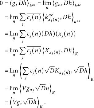 $$ \begin{align*} 0 & = \left\langle {g} , {Dh} \right\rangle_{k^{ac}} = \lim _n \left\langle {g_n} , {Dh} \right\rangle_{k^{ac}} \\ & = \lim _n \sum _j \overline{c_j(n)} \left\langle {k^{ac} _{x_j (n)}} , {Dh} \right\rangle_{k^{ac}} \\ & = \lim _n \sum _j \overline{c_j(n)} (Dh) (x_j (n)) \\ & = \lim _n \sum _j \overline{c_j(n)} \left\langle {K _{x_j (n)}} , {Dh} \right\rangle_K \\ & = \lim _n \left\langle { \sum _j c_j(n) \sqrt{D} K _{x_j (n)}} , {\sqrt{D}h} \right\rangle_K \\ & = \lim _n \left\langle {Vg_n} , {\sqrt{D}h} \right\rangle_K \\ & = \left\langle {Vg} , {\sqrt{D}h} \right\rangle_K. \end{align*} $$
This proves that $Vg \in \mathrm {Ran} \, \sqrt {D} ^{-\| \cdot \| _K}$
is orthogonal to
$Vg \in \mathrm {Ran} \, \sqrt {D} ^{-\| \cdot \| _K}$
is orthogonal to $\sqrt {D} \mathrm {Dom} \, D$
. However,
$\sqrt {D} \mathrm {Dom} \, D$
. However, $\mathrm {Dom} \, D$
is a core for
$\mathrm {Dom} \, D$
is a core for $\sqrt {D}$
, so that
$\sqrt {D}$
, so that $\sqrt {D} \mathrm {Dom} \, D$
is dense in
$\sqrt {D} \mathrm {Dom} \, D$
is dense in $\mathrm {Ran} \, \sqrt {D}$
. This proves that
$\mathrm {Ran} \, \sqrt {D}$
. This proves that $Vg=0$
, and hence
$Vg=0$
, and hence $g=0$
. In conclusion,
$g=0$
. In conclusion, $\mathrm {Ran} \, D \subseteq \mathrm {Ran} \, \mathrm {j} _1 \subseteq \mathcal {H} (k ^{ac} )$
is dense in
$\mathrm {Ran} \, D \subseteq \mathrm {Ran} \, \mathrm {j} _1 \subseteq \mathcal {H} (k ^{ac} )$
is dense in $\mathcal {H} (k^{ac})$
so that both
$\mathcal {H} (k^{ac})$
so that both $\mathrm {j} _1$
and
$\mathrm {j} _1$
and $\mathrm {j} _2$
are isometric embeddings. That is,
$\mathrm {j} _2$
are isometric embeddings. That is, $\mathcal {H} (k^\cap )$
embeds, as a closed, dense subspace of
$\mathcal {H} (k^\cap )$
embeds, as a closed, dense subspace of $\mathcal {H} (k ^{ac})$
, which embeds isometrically into
$\mathcal {H} (k ^{ac})$
, which embeds isometrically into $\mathcal {H} (k)$
and we conclude that
$\mathcal {H} (k)$
and we conclude that $\mathcal {H} (k ^\cap ) = \mathcal {H} (k^{ac})$
so that
$\mathcal {H} (k ^\cap ) = \mathcal {H} (k^{ac})$
so that $k^\cap = k^{ac}$
and
$k^\cap = k^{ac}$
and $\mathfrak {q} _D = \mathfrak {q} _A$
. By the uniqueness of Kato’s Riesz representation of closed, positive semi-definite forms,
$\mathfrak {q} _D = \mathfrak {q} _A$
. By the uniqueness of Kato’s Riesz representation of closed, positive semi-definite forms, $D=A$
as closed operators.
$D=A$
as closed operators.
The fact that $k = k^{ac} + k^s$
, implies that if
$k = k^{ac} + k^s$
, implies that if $\mathrm {e} _{ac} : \mathcal {H} (k^{ac} ) \hookrightarrow \mathcal {H} (k)$
is the isometric embedding and
$\mathrm {e} _{ac} : \mathcal {H} (k^{ac} ) \hookrightarrow \mathcal {H} (k)$
is the isometric embedding and $\mathrm {e} _s : \mathcal {H} (k^s) \hookrightarrow \mathcal {H} (k)$
is the contractive (and injective) embedding, that
$\mathrm {e} _s : \mathcal {H} (k^s) \hookrightarrow \mathcal {H} (k)$
is the contractive (and injective) embedding, that $I = \mathrm {e} _{ac} \mathrm {e} _{ac} ^* + \mathrm {e} _s \mathrm {e} _s ^*$
. Hence
$I = \mathrm {e} _{ac} \mathrm {e} _{ac} ^* + \mathrm {e} _s \mathrm {e} _s ^*$
. Hence $\mathrm {e} _s \mathrm {e} _s ^* = I - P_{ac}$
, so that
$\mathrm {e} _s \mathrm {e} _s ^* = I - P_{ac}$
, so that $\mathcal {H} (k^s)$
also embeds isometrically in
$\mathcal {H} (k^s)$
also embeds isometrically in $\mathcal {H} (k)$
as the orthogonal complement of
$\mathcal {H} (k)$
as the orthogonal complement of $\mathcal {H} (k^{ac} )$
.
$\mathcal {H} (k^{ac} )$
.


 Open access