1 The Falconer distance problem and its many variants

The Falconer distance problem, a continuous analogue of the celebrated Erdős distance problem asks: How large does $\dim (E)$ , for a compact set $E\subseteq \mathbb {R}^d$ , need to be to ensure that the Lebesgue measure of its distance set

$$ \begin{align*}\Delta(E):= \{|x-y|,\, x,y \in E\}\end{align*} $$

is positive? Here and below, $\dim (E)$ denotes the Hausdorff dimension of the set E. Falconer introduced this problem in 1985 in [Reference Falconer10] and established the dimensional threshold $\dim (E)> \frac {d+1}{2}$ .

Further, Falconer conjectured the threshold is $\dim (E)> \frac {d}{2}$ and showed the result could not hold true strictly below that threshold. Falconer’s problem has stimulated much activity and been the focus of many outstanding results (e.g., [Reference Bourgain5–Reference Erdogan9, Reference Guth, Iosevich, Ou and Wang18, Reference Wolff34]).

For two compact sets $E,F \subseteq \mathbb {R}^d$ , one can also consider an asymmetric version, given by

$$ \begin{align*}\Delta(E,F) := \{ |x-y|:\, x\in E, y\in F \},\end{align*} $$

so that $\Delta (E,E)=\Delta (E)$ . Note that all the standard proofs adapt to this setting and the threshold condition can be replaced by a lower bound on $(\dim (E) +\dim (F))/2$ .

Yet another variant of the Falconer problem was introduced by Mattila and Sjölin [Reference Mattila and Sjölin29], who asked how large does $\dim (E)$ need to be in order to ensure that $\Delta (E)$ satisfies the stronger condition of having nonempty interior, and showed that $\dim (E)> \frac {d+1}{2}$ is sufficient.

Both the Falconer and Mattila–Sjölin problems have pinned versions, asking how large does $\dim (E)$ need to be to guarantee that there exists an x such that the pinned distance set,

$$ \begin{align*}\Delta^x(E):= \{|x-y|\, :\, y \in E\},\end{align*} $$

has positive Lebesgue measure or nonempty interior. Peres and Schlag [Reference Peres and Schlag33] showed that this holds for $\dim (E)> \frac {d+2}{2},\, d\ge 3$ (see [Reference Iosevich and Liu22] for some improvements and generalization). More recently, improvements to thresholds in the Falconer distance problem automatically transfer over to the pinned setting due to the magical formula of Liu [Reference Liu26].

Nowadays one can view the original result of Falconer as well as the one of Mattila and Sjölin through the same lens (see, e.g., [Reference Mattila28]). As with Falconer’s original problem, this has led to considerable further work in more general settings [Reference Greenleaf, Iosevich and Taylor14–Reference Greenleaf, Iosevich and Taylor16, Reference Iosevich, Mourgoglou and Taylor23, Reference Koh, Pham and Shen25, Reference Palsson and Romero-Acosta30, Reference Palsson and Romero-Acosta31].

2 A new problem and motivation

In this paper, we introduce new variants of the Falconer and Mattila–Sjölin problems, which we call restricted distance problems.Footnote ¹ These lie between the original distance problems and their pinned variants, and when stated in general encapsulate both of them.

For a compact set $E \subseteq \mathbb {R}^d$ , let $F\subseteq \mathbb {R}^{d}$ be a compact set which might depend on E. Defining the restricted distance set,

$$ \begin{align*}\Delta^F(E) := \{ |x-y|\, : \, x\in F, \,y \in E\},\end{align*} $$

we ask what lower bounds on $\dim (E)$ guarantee that $\Delta ^F(E)$ has positive Lebesgue measure or nonempty interior. Note that if F has no dependence on E, then ${\Delta ^F(E)=\Delta (E,F)}$ and one is in the asymmetric setting of the Falconer or Mattila–Sjölin problem.

The two simplest cases of a set F which is dependent on E are the extremes when

(i) $F=E$ , so that $\Delta ^F(E)=\Delta (E)$ , the standard distance set of E,

and

(ii) $F=\{x_0\}$ for some point $x_0$ , fixed in advance. This is similar to a pinned distance problem, but stronger than the usual one, since the pin is fixed. (A result giving nonempty interior for the set of volumes of parallelepipeds generated by an arbitrary $x_0$ and all d-tuples of points in $E\subset \mathbb {R}^d$ is in [Reference Greenleaf, Iosevich and Taylor15, Theorem 1.2], where this is referred to as a strongly pinned result.)

To illustrate the type of restricted distance problems in which we are interested, we focus on a prototype lying between (i) and (ii). For a compact set $E\subseteq \mathbb {R}^d$ , let ${F=\{\,(x,x)\,:\, x\in E\,\}\subset \mathbb {R}^{2d}}$ , the diagonal of $E\times E$ . With $|\, \cdot \,|$ denoting the Euclidean norm on $\mathbb {R}^{2d}$ , we ask what lower bound on $\dim (E)$ ensures that

(2.1) $$ \begin{align} \Delta^F(E\times E)= \{ \,\left|\,(x,x)-(y_1,y_2)\,\right| : x, y_1, y_2\, \in E \}, \end{align} $$

which we will also denote by $\Delta ^{\mathrm{diag}}(E)$ , has positive Lebesgue measure or nonempty interior in $\mathbb {R}$ . See Figure 1.

Figure 1: A sketch of how one could view $\Delta ^{\mathrm{diag}}(E)$ .

As noted in [Reference Borges, Iosevich and Ou4], in order to make the problem more interesting, in (2.1), one should impose a condition $y_1\ne y_2$ because, if $y_1=y_2$ were allowed, then $\Delta ^{\mathrm{diag}}(E)\supset \sqrt 2\cdot \Delta (E)$ , which would then have positive Lebesgue measure or nonempty interior if $\dim (E)$ is greater than the thresholds in $\mathbb {R}^d$ for the standard Falconer or Mattila–Sjölin distance problems, respectively. We thus include this condition and its extensions in the statements below. So, we define F

$$ \begin{align*}\mathring{\Delta}^{\mathrm{diag}}(E):= \{ \,\left|\,(x,x)-(y_1,y_2)\,\right| : x, y_1, y_2\, \in E,\, y_1\ne y_2\, \}.\end{align*} $$

or an $E\subset \mathbb {R}^d$ and an $F\subset \mathbb {R}^{ld}$ , define

$$ \begin{align*}\mathring{\Delta}^F(E):=\left\{ \, |x-y|\, :\, x\in F,\, y=(y_1,\dots,y_l)\in E^l,\, y_i\ne y_j,\, \forall i\ne j\, \right\}, \end{align*} $$

where $|\, \cdot \, |$ is the Euclidean norm on $\mathbb {R}^{ld}$ .

We are now ready to pose the following set of questions generalizing the prototype:

Restricted Falconer and Mattila–Sjölin Problems. Fix $l\in \mathbb N$ and a map $\mathcal F$ from the collection $\mathcal C\left (\mathbb {R}^d\right )$ of compact sets in $\mathbb {R}^d$ to $2^{\mathcal C\left (\mathbb {R}^{ld}\right )}$ , denoting the image of a compact E by $\mathcal F_E$ .

Q. What lower bounds on $\dim (E)$ ensure that either

(i) there exists an $F \in \mathcal {F}_E$ such that $\mathring {\Delta }^F(E)$ has positive Lebesgue measure (or nonempty interior); or

(ii) for a.e. $F\in \mathcal {F}_E$ (with respect to some measure on $\mathcal F$ ); or

(iii) for every $F\in \mathcal {F}_E$ ,

the same property holds.

Remarks 1. For $l=1$ , case (i), and positive Lebesgue measure, the choice of $\mathcal {F}_E=\{E\}$ yields the classical Falconer distance problem, while $\mathcal {F}_E=\{ \{x\}:\, x\in E\}$ yields its standard pinned variant. On the other hand, $\mathring {\Delta }^{\mathrm{diag}}(E)$ corresponds to $l=2$ , $\mathcal F_E=\{F\}$ , where F is the diagonal of $E\times E$ in $\mathbb {R}^{2d}$ . If $\mathcal F$ is a singleton, the questions (i), (ii), and (iii) collapse into one, concerning a three-point configuration problem of either Falconer or Mattila–Sjölin type, and in this paper we will focus on this, for $\mathring {\Delta }^{\mathrm{diag}}(E)$ and its k-point configuration generalizations.

2. $\mathbb {R}^d$ can be replaced by a smooth d-dimensional manifold with a smooth density, and Theorem 3.3 below is formulated in this setting.

3. Returning to the prototype (2.1), note that if we do not restrict to the diagonal but instead consider the full $\mathbb {R}^{2d}$ distance set $\Delta (E\times E)$ , the best results known for the $\mathbb {R}^{2d}$ Falconer problem would yield a sufficient lower bound on $\dim (E)$ . Since $\dim (E)>\frac {d}{2}+ \frac {1}{8}$ implies that $\dim (E\times E)> \frac {2d}2+\frac {1}{4}$ , and $2d$ is even, the results of [Reference Du, Iosevich, Ou, Wang and Zhang7, Reference Guth, Iosevich, Ou and Wang18] yield that $\Delta (E\times E)$ has positive Lebesgue measure. However, for the restricted Falconer problem we are considering, the set $\mathring {\Delta }^{\mathrm{diag}}(E)$ consists only of distances from points on the diagonal of E to general points of $E\times E$ .

4. By a result of Peres and Schlag [Reference Peres and Schlag33], if $\dim (E)>(d+2)/2$ , with $d\ge 3$ , then there exists an x such that the pinned distance set $\Delta ^x(E)=\{\, |x-y_1|\, :\, y_1\in E\, \}$ contains an interval. This immediately implies that $\mathring {\Delta }^{\mathrm{diag}}(E)$ contains an interval, since $y_2$ in (2.1) can simply be fixed. The same principle applies to any $\mathring {\Delta }^{F}(E)$ with F of the form

(2.2) $$ \begin{align} F=\{(x,\phi_2(x),\dots,\phi_l(x))\, :\, x\in E\}, \end{align} $$

with arbitrary continuous functions $\phi _j:\mathbb {R}^d\to \mathbb {R}^d$ . Further comments are in Section 3.1. below. However, this argument relies on both the form of F and the product nature of the Euclidean metric on $\mathbb {R}^{ld}$ , and thus does not apply to our most general result, Theorem 3.3.

3 The main results

Our main results are the following, in increasing order of generality.

Theorem 3.1 is the $k=3$ case of the following theorem.

Theorem 3.2 Let $E\subseteq \mathbb {R}^d$ be compact, $d\ge 2$ . For $k\ge 3$ , define the k-point configuration set,

$$ \begin{align*}\mathring{\Delta}_k^{\mathrm{diag}}(E):=\left\{\, \left|\, (x,\dots,x) - \left(y_1,\dots, y_{k-1}\right)\, \right|\, : \, x, y_1,\dots, y_{k-1}\in E ,\, y_i\ne y_j \right\},\end{align*} $$

$|\, \cdot \, |$ being the Euclidean norm on $\mathbb {R}^{(k-1)d}$ . Then ${\mathop {}\!\mathrm {Int}} ( \mathring {\Delta }_k^{\mathrm{diag}} (E)) \neq \varnothing $ if

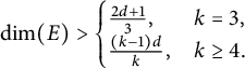
(3.1) $$ \begin{align} \dim(E)> \begin{cases} \frac{2d+1}{3}, & k=3, \\ \frac{(k-1)d}k, & k\ge 4. \end{cases} \end{align} $$

In fact, the Euclidean structure is not necessary. More generally, we have the following theorem.

Theorem 3.3 Suppose $d\ge 2$ and $k\ge 3$ . Let $\mathcal G$ denote the space of $C^\omega $ Riemannian metrics on $\left (\mathbb {R}^d\right )^{k-1}$ . For any $g\in \mathcal G$ , let $d_g$ be the induced distance function, which is defined on at least a neighborhood of the diagonal of $\left (\mathbb {R}^d\right )^{k-1}$ . Let $g_0$ denote the Euclidean metric. Then there is an $N=N_{d,k}\in \mathbb N$ and a neighborhood $\mathcal U$ of $g_0$ in the $C^N$ topology on $\mathcal G$ such that if $g\in \mathcal U$ , and for a compact $E\subset \mathbb {R}^d$ , we define

$$ \begin{align*} \mathring{\Delta}_g^{\mathrm{diag}}(E)~:=~& \big\{ \, d_g\left(\left(x,\dots,x\right),\left(y_1,\dots,y_{k-1}\right)\right)\, \\ & \qquad\quad :\, x,y_1,\dots, y_{k-1} \in E,\, y_i\ne y_j,\, \forall\, i\ne j \big\}, \end{align*} $$

then ${\mathop {}\!\mathrm {Int}} ( \mathring {\Delta }^{\mathrm{diag}} (E)) \neq \varnothing $ if (3.1) holds.

4 The bilinear spherical averaging operator

Let $d\geq 2$ . Then, for $x\in \mathbb {R}^d$ , $t>0$ , and for functions $f,g \in \mathcal {S} (\mathbb {R}^d)$ , define the bilinear spherical averaging operator,

$$ \begin{align*}A_r(f,g)(x):= \int_{\mathbb{S}^{2d-1}} f(x-ru)\,g(x-rv)\, d\sigma(u,v),\end{align*} $$

where $\sigma $ is the standard surface measure on unit sphere $\mathbb {S}^{2d-1}$ in $\mathbb {R}^{2d}$ ,

$$ \begin{align*}\mathbb{S}^{2d-1}=\{ (u,v) \in \mathbb{R}^d \times \mathbb{R}^d\, :\, |u|^2+|v|^2=1\, \}.\end{align*} $$

Next, we define the (full) maximal bilinear spherical operator

$$ \begin{align*}\mathcal{M}(f,g)(x):= \sup_{r>0}|A_r(f,g)(x)|,\end{align*} $$

as well as its single-scale (localized) version,

$$ \begin{align*}\widetilde{\mathcal{M}}(f,g)(x):= \sup_{r\in [1,2]}|A_r(f,g)(x)|.\end{align*} $$

4.1 Known results and goals

The operators $A_r$ and $\mathcal {M}$ first appeared in the paper of Geba et al. [Reference Geba, Greenleaf, Iosevich, Palsson and Sawyer11], where the authors proved some initial $L^p$ improving estimates for these operators. Subsequently, the $L^p$ improving estimates for $\mathcal {M}$ were further developed in the works of Barrionevo et al. (see [Reference Barrionuevo, Grafakos, He, Honzík and Oliveira1]), Grafakos, He, and Honzík (see [Reference Grafakos, He and Honzík13]), and Heo, Hong, and Yang (see [Reference Heo, Hong and Yang19]). Finally, the full region $L^p$ improving estimates for the operator $\mathcal {M}$ were given in the work of Jeong and Lee (see [Reference Jeong and Lee24]) as the result of a clever “slicing” argument enabled them to pointwisely dominate the maximal bilinear spherical averaging operator by the product of a Hardy–Littlewood maximal operator and a linear spherical averaging operator, both of which have been extensively studied. Furthermore, in the same work, the authors explored the $L^p$ improving estimates for the operator $\widetilde {\mathcal {M}}$ obtaining a large region of exponents; however, there is still work left open in this case. Subsequent developments have included sparse domination results [Reference Borges, Foster, Ou, Pipher and Zhou3, Reference Palsson and Sovine32] and very recent lacunary maximal operator results [Reference Borges and Foster2].

We already know the operator is bounded from $L^2\times L^2 \to L^2$ , but this is not enough. For our work, rather than $L^p$ improving estimates for $A_r$ , we need ${L^2\times L^2 \to L^2}$ estimates with decay in the frequency variable. The key to achieve this is to exploit the decay of the surface measure on the unit ball in $\mathbb {R}^{2d}$ and work on dyadic scales.

A key ingredient in the proof of Theorem 3.1 will be the following:

Proposition Let $i, j \in \mathbb {N}$ , and let $f,g$ be functions with

$$ \begin{align*}\mathrm{supp}(\hat{f}) \subset \{\xi \in \mathbb{R}^d \, :\, 2^{i-1}<|\xi| \leq 2^{i+1}\}\end{align*} $$

and

$$ \begin{align*}\mathrm{supp}(\hat{g}) \subset \{\xi \in \mathbb{R}^d \, :\, 2^{j-1}<|\xi| \leq 2^{j+1}\},\end{align*} $$

then

$$ \begin{align*}\|A_r(f,g)\|_2 \lesssim_r \big(2^{2i}+2^{2j}\big)^{-\frac{2d-1}{4}} 2^{\min \{i,j\} \frac{d}{2}} \|f\|_2 \|g\|_2.\end{align*} $$

Let $\sigma _r$ to be the surface measure on the sphere of radius r in $\mathbb {R}^{d}\times \mathbb {R}^d$ :

$$ \begin{align*}\mathbb{S}_r^{2d-1}=\{ (u,v) \in \mathbb{R}^d \times \mathbb{R}^d\, :\, |u|^2+|v|^2=r^2\, \},\end{align*} $$

so that $\sigma =\sigma _1$ and, by a change of variable, one has

$$ \begin{align*}A_r(f,g)(x)= \frac{1}{r^{2d-1}}\,\int_{\mathbb{S}_r^{2d-1}} f(x-u)\,g(x-v)\, d\sigma_r(u,v).\end{align*} $$

As a tool in the proof of Proposition 4.1, we note the Fourier decay of these measures. For $(\xi ,\eta ) \in \mathbb {R}^d\times \mathbb {R}^d$ , by the dilation property of the Fourier transform and stationary phase, respectively, one has

(4.1)

For the purpose of proving Proposition 4.1, we may assume that $\hat {f}$ and $\hat {g}$ , besides being compactly supported, are smooth. Thus, for $\xi \in \mathbb {R}^d$ , we use Fourier inversion formula and Fubini’s theorem, justified since $\hat {f},\hat {g}\in C_0^\infty $ , to calculate

Since

$$ \begin{align*}\int_{\mathbb{R}^d}\, e^{2\pi i(x,x,x)\cdot (\eta, -\xi, x')} \,dx = \delta(\eta-\xi+x'),\end{align*} $$

where $\delta (\cdot )$ is the delta distribution on $\mathbb {R}^d$ , this gives the representation

We can now prove Proposition 4.1.

Proof Without loss of generality, we can assume that $i\leq j$ . Applying Plancherel and the identity above yields

The Fourier decay of the measure in (4.1) gives

$$ \begin{align*}\lesssim_r \big(2^{2i}+2^{2j}\big)^{-\frac{2d-1}{2}} \int_{\mathbb{R}^d} \Big( \int_{\mathbb{R}^d}|\widehat{f}(\eta)|\,|\widehat{g}(\xi-\eta)|\, d\eta \Big)^2 d\xi \end{align*} $$

since $|\eta |\sim 2^i$ , $|\xi -\eta |\sim 2^j$ , and so $|(\eta , \xi -\eta )|^2= |\eta |^2+|\xi -\eta |^2 \sim 2^{2i}+2^{2j}$ .

Next, let $A^{\xi }_{i,j}:=\{\eta \, : \, |\eta |\sim 2^i\,,\, |\xi -\eta |\sim 2^j \}$ . Note that the inner integral is supported on this set and so we can estimate it by Cauchy–Schwarz:

$$ \begin{align*}\int_{A^{\xi}_{i,j}}|\widehat{f}(\eta)|\,|\widehat{g}(\xi-\eta)|\, d\eta \lesssim 2^{\frac{id}{2}} \Bigg(\int_{\mathbb{R}^d} \, |\widehat{f}(\eta)|^2 \, |\widehat{g}(\xi-\eta)|^2 d \eta\Bigg)^{\frac{1}{2}},\end{align*} $$

which gives, after applying Fubini’s theorem (again justified since $\hat {f}, \hat {g}\in C_0^\infty $ ) and a change of variable:

$$ \begin{align*}\|A_r(f,g)\|^2_2 \lesssim_r \big(2^{2i}+2^{2j}\big)^{-\frac{2d-1}{2}} \, 2^{id} \|f\|_2^2\|g\|_2^2\end{align*} $$

This finishes the proof of Proposition 4.1.

5 Proof of Theorem 3.1

In this section, we prove Theorem 3.1 using the estimates for the bilinear spherical averaging operator $A_r$ in Proposition 4.1.

Proof Let $E\subset \mathbb {R}^d$ with $\dim (E)>\frac {2d+1}{3}$ , and fix an $s\in (\frac {2d+1}{3}, \dim (E))$ . We argue as in the proof of Theorem 4.6 in [Reference Mattila28]. By Frostman’s lemma [Reference Mattila28, Theorem 2.8], there exists a measure $\mu \in \mathcal {M}(E)$ with $I_s(\mu ) < \infty $ . This then induces the distance measure, $\nu _\mu \in \mathcal {M}(\mathring {\Delta }^{\mathrm{diag}}(E))$ , which is the image (or pushforward) of $\mu \times \mu \times \mu $ under the distance map (or configuration function)

$$ \begin{align*}E\times E\times E \owns (x,y_1,y_2) \to \left|(x,x)-(y_1,y_2)\right|\in \mathbb{R}.\end{align*} $$

More explicitly, for a Borel set $B\subset \mathbb {R}$ ,

$$ \begin{align*}\nu_\mu(B):= (\mu\times\mu\times \mu) \left( \left\{(x,y_1,y_2)\, :\, |(x,x)-(y_1,y_2)| \in B\right\} \right).\end{align*} $$

We have seemingly enlarged the set being measured by including the set $y_1=y_2$ , but note that, for any x, $(\mu \times \mu )\left (\left \{(y_1,y_2):y_1=y_2\right \}\right )=0$ . This follows from the fact that in $\mathbb {R}^{2d}$ , $\dim \left (\{y_1=y_2\}\right )=d$ , of dimension strictly less than $\dim (E\times E)$ , since, by [Reference Mattila28, Theorem 2.10],

$$ \begin{align*}\dim(E\times E)\ge 2\dim(E)>(4d+2)/3 > d.\end{align*} $$

Equivalently, for a continuous function g on $\mathbb {R}$ ,

$$ \begin{align*}\int_{\mathbb{R}} g(r) \, d\nu_\mu(r)= \int_E \,\int_E\,\int_E g\big( |(x,x)-(y_1,y_2)| \big)\, d\mu(x) \, d\mu(y_1)\, d\mu(y_2).\end{align*} $$

Next, we claim that, for an $f\in C_0^\infty \left (\mathbb {R}^d\right )$ , $\nu _f:=\nu _{f\cdot dx}$ is also a function. To see this, write

$$ \begin{align*} \int_{\mathbb{R}} g(r) \, d\nu_f(r)&= \int_{\mathbb{R}^d} \,\int_{\mathbb{R}^d}\,\int_{\mathbb{R}^d} g\big( |(x,x)-(y_1,y_2)| \big) f(x)\, f(y_1)\,f(y_2)\, dx\, dy_1\, dy_2 \\ &= \int_{\mathbb{R}^{2d}} \int_{\mathbb{R}^d} g\big( |(x,x)-y| \big) (f\otimes f)(y)\, f(x)\, dx\,dy \\ &= \int_{\mathbb{R}} \int_{\mathbb{S}^{2d-1}} \!\int_0^{\infty} \!g(r) \, f(x-r \omega_1) \, f(x-r\omega_2) \, r^{2d-1}\,dr\, d\sigma(\omega) \, f(x) dx, \end{align*} $$

where in the second equality for $y=(y_1,y_2)\in \mathbb {R}^{d} \times \mathbb {R}^{d} $ we write $(f\otimes f)(y):=f(y_1)\, f(y_2)$ , and in the third equality, we used polar coordinates, with $\omega =(\omega _1,\omega _2)\in \mathbb {S}^{2d-1}$ . Therefore, after applying Fubini’s theorem (justified by $f\in C_0^\infty $ ) and using the definition of the bilinear spherical averaging operator $A_r$ , we obtain

$$ \begin{align*}\int_0^{\infty} g(r)\, d\nu_f(r)= \int_0^{\infty} g(r) \,r^{2d-1}\, A_r(f,f)(x) \, f(x)\, dx\, dr,\end{align*} $$

which implies that $\nu _f$ is a function, with

$$ \begin{align*}\nu_f(r)= r^{2d-1}\,\int_{\mathbb{R}^d} A_r(f,f)(x) \, f(x) \, dx.\end{align*} $$

Next, we approximate weakly the Frostman measure $\mu $ : Let $\psi \in C_0^\infty (\mathbb {R}^d)$ with ${\int \psi =1}$ , and for $\epsilon>0$ , define $\psi _{\epsilon }(x)=\epsilon ^{-d}\psi (\frac {x}{\epsilon })$ . Then, setting $\mu _{\epsilon } := \psi _{\epsilon } \ast \mu $ , we have $\mu _{\epsilon } \to \mu $ weakly as $\epsilon \to 0$ , and so $\nu _{\mu _{\epsilon }} \to \nu _\mu $ weakly, as well. Moreover, $\widehat {\mu _{\epsilon }}(x)=\widehat {\psi }(\epsilon \,x) \, \widehat {\mu }(x) \to \widehat {\mu }(x)$ for all $x\in \mathbb {R}^d$ .

For any $\epsilon>0$ , $\mu _{\epsilon }$ , is a function; thus, applying the formula above for $\nu _f$ , we get

$$ \begin{align*}\nu_{\mu_{\epsilon}}(r)= r^{2d-1}\,\int_{\mathbb{R}^d} \, A_r(\mu_{\epsilon},\mu_{\epsilon})(x) \, \mu_{\epsilon}(x) dx,\end{align*} $$

and by the comments above, the left side converges weakly to $\nu _{\mu }(r)$ . We would like to see what the right-hand side converges to. Using Parseval’s theorem, we see

Next, we have pointwise, and since

we get

with passing the limit inside justified by the dominated convergence theorem. Note that

$$ \begin{align*}|\widehat{\mu}(\eta) \, \widehat{\mu}(\xi-\eta)\, \widehat{\sigma}(r(\eta,\xi-\eta))| &\lesssim _r |\widehat{\mu}(\eta) \, \widehat{\mu}(\xi-\eta)||(\eta, \xi-\eta)|^{-\frac{2d-1}{2}} \\ &\lesssim_r |\widehat{\mu}(\eta) \, \widehat{\mu}(\xi-\eta)|\, |\eta|^{-\frac{2d-1}{4}} \, |\xi-\eta|^{-\frac{2d-1}{4}} \end{align*} $$

and the last function is integrable (in $\eta $ ) by utilizing the Cauchy–Schwarz inequality, a change of variable, and the fact $I_{\frac {1}{2}}(\mu ) \leq I_s(\mu )$ , since $\mu $ has compact support and $s> \frac {1}{2}$ .

Now we write

$$ \begin{align*}\nu_{\mu_{\epsilon}}(r)=r^{2d-1}\,\int_{\mathbb{R}^d} \,B_{\epsilon}(\xi)\, E_{\epsilon}(\xi)\, d \xi,\end{align*} $$

where

$$ \begin{align*}B_{\epsilon}(\xi)= |\xi|^{\frac{d-s}{2}}\int_{\mathbb{R}^d} \widehat{\psi}(\epsilon\,\eta \, )\widehat{\mu}(\eta) \,\widehat{\psi}(\epsilon\,(\xi-\eta)) \, \widehat{\mu}(\xi-\eta)\, \widehat{\sigma}(r(\eta,\xi-\eta))\, d\eta\end{align*} $$

and

$$ \begin{align*}E_{\epsilon}(\xi) = |\xi|^{\frac{s-d}{2}}\widehat{\psi}(\epsilon\,\xi)\, \widehat{\mu}(\xi).\end{align*} $$

We will dominate each of these functions by $L^2$ integrable functions, independently of $\epsilon $ , so that $B_{\epsilon }(\xi )\, E_{\epsilon }(\xi )$ will be dominated by an $L^1$ function, independently of $\epsilon $ ; this will allow us to use the dominated convergence theorem, yielding the formula

(5.1) $$ \begin{align} \nu_\mu(r)= r^{2d-1}\int_{\mathbb{R}^d}\Bigg( \int_{\mathbb{R}^d} \widehat{\mu}(\eta) \, \widehat{\mu}(\xi-\eta)\, \widehat{\sigma}(r\eta,r(\xi-\eta))\, d\eta \Bigg) \widehat{\mu}(\xi) d\xi. \end{align} $$

Note first that

$$ \begin{align*}|E_{\epsilon}(\xi)| = |\xi|^{\frac{s-d}{2}}|\widehat{\psi}(\epsilon\,\xi)\, \widehat{\mu}(\xi)| \lesssim_{\psi} |\xi|^{\frac{s-d}{2}}\,| \widehat{\mu}(\xi)|\end{align*} $$

and the $L^2$ norm of the right side is exactly equal to $I_s(\mu )$ which is finite. Second,

$$ \begin{align*}|B_{\epsilon}(\xi)| \lesssim_{\psi} |\xi|^{\frac{d-s}{2}}\int_{\mathbb{R}^d} |\widehat{\mu}(\eta)| \, |\widehat{\mu}(\xi-\eta)|\, |\widehat{\sigma}(r(\eta,\xi-\eta))|\, d\eta.\end{align*} $$

Now we will decompose $\hat {\mu }$ on dyadic scales. Consider the Schwartz functions $\eta _0 (\xi )$ supported at $|\xi | \leq \frac {1}{2}$ and $\eta (\xi )$ supported in the spherical shell $\frac {1}{2}<|\xi |\leq 2$ such that the quantities $ \eta _0(\xi )$ , $ \eta _j(\xi ):= \eta \big (2^{-j}\xi \big )$ , with $j \geq 1$ , form a partition of unity.

Then we define and so $ \widehat {\mu }_j(\xi )= \widehat {\mu }(\xi ) \eta _j(\xi )$ . Thus, $\widehat {\mu }(\xi )=\sum \limits _{j=0}^{\infty } \widehat {\mu _j}(\xi )$ and, moreover,

$$ \begin{align*} |B_{\epsilon}(\xi)| &\lesssim_{\psi} \sum\limits_{i,j=0}^{\infty} |\xi|^{\frac{d-s}{2}}\int_{\mathbb{R}^d} |\widehat{\mu_i}(\eta)| \, |\widehat{\mu_j}(\xi-\eta)|\, |\widehat{\sigma}(r(\eta,\xi-\eta))|\, d\eta \\ &\lesssim \sum\limits_{i,j=0}^{\infty} (2^i+2^j)^{\frac{d-s}{2}} \int_{\mathbb{R}^d} |\widehat{\mu_i}(\eta)| \, |\widehat{\mu_j}(\xi-\eta)|\, |\widehat{\sigma}(r(\eta,\xi-\eta))|\, d\eta \end{align*} $$

since $|\xi | \leq |\eta |+|\xi -\eta |\lesssim 2^i+2^j$ on the supports of $\widehat {\mu _i}, \widehat {\mu _i}$ and $d>s$ . Now the function on the right is independent of $\epsilon $ and $L^2$ integrable as

$$ \begin{align*}I:=\bigg(\int_{\mathbb{R}^d}\, \Bigg( \sum\limits_{i,j=0}^{\infty} (2^i+2^j)^{\frac{d-s}{2}} \int_{\mathbb{R}^d} |\widehat{\mu_i}(\eta)| \, |\widehat{\mu_j}(\xi-\eta)|\, |\widehat{\sigma}(r(\eta,\xi-\eta))|\, d\eta\, \Bigg)^2 \, d\xi \bigg)^{\frac{1}{2}}\end{align*} $$

$$ \begin{align*}\leq \sum\limits_{i,j=0}^{\infty} (2^i+2^j)^{\frac{d-s}{2}} \bigg(\int_{\mathbb{R}^d}\, \Bigg(\int_{\mathbb{R}^d} |\widehat{\mu_i}(\eta)| \, |\widehat{\mu_j}(\xi-\eta)|\, |\widehat{\sigma}(r(\eta,\xi-\eta))|\, d\eta\, \Bigg)^2 \, d\xi \bigg)^{\frac{1}{2}}\end{align*} $$

$$ \begin{align*}\lesssim_r \sum\limits_{i,j=0}^{\infty} (2^i+2^j)^{\frac{d-s}{2}} \big(2^{2i}+2^{2j}\big)^{-\frac{2d-1}{4}} 2^{\min \{i,j\} \frac{d}{2}} \|\mu_i\|_2 \|\mu_j\|_2\end{align*} $$

by Minkowski’s integral inequality and Proposition 4.1.

Next, we want to evaluate the $L^2$ -norms of the functions $\mu _i$ . We have, using Plancherel’s theorem in the first line and the Fourier transform characterization of the energy integral [Reference Mattila28, Theorem 3.10] in the third line,

$$ \begin{align*} \|\mu_{i}\|_2^2 =\|\widehat{\mu_{i}}\|_2^2 &\lesssim 2^{i(d-s)} \int_{\mathbb{R}^d} |\xi|^{-d+s} |\widehat{\mu_{i}}(\xi)|^2 d\xi \\ &\lesssim_{\eta} 2^{i(d-s)}\int_{\mathbb{R}^d} |\xi|^{-d+s} |\widehat{\mu}(\xi)|^2 d\xi \\ &= 2^{i(d-s)}I_s(\mu) \\ &\lesssim_{\mu} 2^{i(d-s)}. \end{align*} $$

With this at hand, we continue estimating I by utilizing the symmetry of the summand,

$$ \begin{align*} I &\lesssim \sum\limits_{i=0}^{\infty} \sum\limits_{j=i}^{\infty} 2^{j\frac{d-s}{2}} \, 2^{-j\frac{2d-1}{2}} \, 2^{i\frac{d}{2}} \, 2^{i\frac{d-s}{2}}\, 2^{j\frac{d-s}{2}} \\ &= \sum\limits_{i=0}^{\infty} 2^{i(d -\frac{s}{2})} \sum\limits_{j=i}^{\infty} 2^{j(\frac{1}{2} -s)}\\ &\lesssim\sum\limits_{i=0}^{\infty} 2^{i(d -\frac{s}{2})} \, 2^{i(\frac{1}{2} -s)}, \end{align*} $$

which is finite since $s> \frac {2d+1}{3}$ .

Therefore, for a set E with $\dim (E)> \frac {2d+1}{3}$ , from the dominated convergence theorem, it follows that the function in (5.1) is continuous in r. Finally, since $\mathrm{supp} (\nu _\mu ) \subset {\Delta }^{\mathrm{diag}}(\mathrm{supp} (\mu )) \subset {\Delta }^{\mathrm{diag}}(E)$ , we see that $\mathring {\Delta }^{\mathrm{diag}}(E)$ has non-empty interior.

Remark 5.1 The same proof works for an arbitrary number of points. Namely, for $k\geq 3$ , if for $E\subset \mathbb {R}^d$ compact we define the k-point configuration set $\mathring {\Delta }_k^{\mathrm{diag}}(E)$ as in Theorem 3.2, then

$$ \begin{align*} \dim(E)> \frac{(k-1)d+1}{k}\ \text{implies that}\ {\mathop{}\!\mathrm{Int}} ( \mathring{\Delta}_k^{\mathrm{diag}} (E)) \neq \varnothing, \end{align*} $$

extending what we have just shown for $k=3$ . However, as we show in the next section, it turns out that using the FIO approach of [Reference Greenleaf, Iosevich and Taylor14, Reference Greenleaf, Iosevich and Taylor15] allows one to lower this by $1/k$ for $k\ge 4$ . Additionally, the FIO approach does not require the metric to be Euclidean, or a product, or even translation invariant, leading to Theorem 3.3.

6 A Fourier integral operator approach

We now prove Theorem 3.2 using multilinear FIOs, improving on the threshold, mentioned in Remark 5.1, which can be obtained for $k\ge 4$ by Fourier transform methods.

The FIO method, introduced in [Reference Greenleaf, Iosevich and Taylor14] for two-point configuration sets and then extended to k-point configurations in [Reference Greenleaf, Iosevich and Taylor15], is based on optimizing linear FIO estimates over all bipartite partitions of the variables. The flexibility of this approach and its stability under perturbations then sets the scene for the proof of Theorem 3.3.

We will give the calculations needed to prove Theorem 3.2, using the general framework and notation of [Reference Greenleaf, Iosevich and Taylor15], which the reader should consult for a full exposition. In the terminology of [Reference Grafakos, Greenleaf, Iosevich and Palsson12], the k-configuration set $ \mathring {\Delta }_k^{\mathrm{diag}} (E)$ is a $\Phi $ -configuration set. For convenience, we relabel $(x,y_1,\dots ,y_{k-1})$ as $(x^0,x^1,\dots ,x^{k-1})$ and define $\Phi :(\mathbb {R}^d)^k\to \mathbb {R}$ ,

(6.1) $$ \begin{align} \Phi(x^0,x^1,\dots,x^{k-1})=\frac12\sum_{i=1}^{k-1} \big| x^0-x^i \big|^2, \end{align} $$

so that ${\mathop {}\!\mathrm {Int}} ( \mathring {\Delta }^{\mathrm{diag}}_k (E)) \neq \varnothing $ iff

$$ \begin{align*}\mathring{\Delta}_\Phi(E):=\left\{\Phi\left(x^0,x^1,\dots ,x^{k-1}\right): x^0,\dots, x^{k-1}\in E, x_i\ne x_j,\, \forall i\ne j\right\},\end{align*} $$

has nonempty interior.

We start by finding a base point in $\mathbb {R}^{kd}$ about which to work. Let $s_0=s_0(d,k)$ be the threshold for $\dim (E)$ in (3.1) in the statement of Theorem 3.2, and suppose ${\dim (E)>s_0}$ . Pick an s with $s_0<s<\dim (E)$ , and let $\mu $ be a Frostman measure supported on E and of finite s-energy (see [Reference Mattila27, Theorem 8.17]). We claim that there exist points $x_0^0,\dots ,x_0^{k-1}\in E$ and an $\epsilon>0$ such that $\mu (B(x_0^i,\epsilon ))>0,\, 0\le i\le k-1$ ,

$$ \begin{align*}x_0^i\ne x_0^0,\, \forall\, i>0,\text{ and } x_0^i\ne x_0^j,\, \forall\, 1\le i\ne j\le k-1,\end{align*} $$

and then set

(6.2) $$ \begin{align} t_0:=\frac12\sum_{i=1}^{k-1} \left|x_0^0-x_0^i\right|{}^2>0. \end{align} $$

To see this, one can argue as in [Reference Greenleaf, Iosevich and Taylor15, Section 4.1]. The key point is that if we define

(6.3) $$ \begin{align} W:=\left\{(x^0,\dots,x^{k-1})\in\mathbb{R}^{kd}\, :\, x^i\ne x^0,\, \forall\, i>0,\text{ and } x^i\ne x^j,\, \forall\, 1\le i\ne j\le k-1\,\right\}, \end{align} $$

then W is a Zariski open subset of $\mathbb {R}^{kd}$ , whose complement is contained in a union of algebraic varieties of dimensions $\le (k-1)d$ (since each $\{x^i=x^j\}$ is codimension d). Hence, $\dim \left (\mathbb {R}^{kd}\setminus W\right )\le (k-1)d<s$ , so that $(\mu \times \cdots \times \mu )(\mathbb {R}^{kd}\setminus W)=0$ . See [Reference Greenleaf, Iosevich and Taylor15], where this type of argument is given for several different $\Phi $ -configurations, for more details.

For each $t>0$ , the configuration function $\Phi $ induces a surface measure,

$$ \begin{align*}K_t(x^0,\dots,x^{k-1})=\delta\left(\Phi\left(x^0,\dots,x^{k-1}\right) - t \right)\in\mathcal D'\left(\mathbb{R}^{kd}\right),\end{align*} $$

where $\delta (\cdot )$ is the delta distribution on $\mathbb {R}$ . Each $K_t$ supported on its incidence relation,

(6.4) $$ \begin{align} Z_t:=\left\{\, \left(x^0,\dots,x^{k-1}\right)\in\mathbb{R}^{kd}\, :\, \Phi(x^0,\dots,x^{k-1})=t\,\right\}, \end{align} $$

and is a Fourier integral (or Lagrangian) distribution on $\mathbb {R}^{kd}$ in the sense of Hörmander [Reference Hörmander20, Reference Hörmander21]: by Fourier inversion of $\delta $ on $\mathbb {R}$ , $K_t$ has an oscillatory representation,

$$ \begin{align*}K_t(\cdot)=c\int_{\mathbb{R}} e^{i\tau\left(\Phi(x^0,\dots,x^{k-1})-t\right)} 1(\tau)\, d\tau.\end{align*} $$

The phase function parametrizes the conormal bundle of $Z_t$ , denoted $N^*Z_t\subset T^*\left (\mathbb {R}^{kd}\right )\setminus 0$ , which is a Lagrangian submanifold, while the amplitude $1(\tau )$ is a symbol of order 0. Thus, by Hömander’s formula for the order of a Fourier integral distribution,

$$ \begin{align*}\mathrm{ord}(K_t)=\mathrm{ord}(1(\cdot))+\frac{\#\text{ phase vars}}2-\frac{\#\text{ spatial vars}}4=0+\frac12-\frac{kd}4\end{align*} $$

and one writes $K_t\in I^{\frac 12-\frac {kd}4}\left (N^*Z_t\right )$ .

For convenience, we will write $N^*Z_t$ with each pair of spatial and cotangent variables, $(x^i,\, \xi ^i)$ , grouped together. Thus,

(6.5) $$ \begin{align} N^*Z_t =& \Bigg\{ \left(x^0,\tau\sum_{i=1}^{k-1}(x^0-x^i); x^1,-\tau(x^0-x^1); \dots; x^{k-1},-\tau(x^0-x^{k-1})\right) \nonumber\\ & \qquad :\, \left(x^0,\dots,x^{k-1}\right)\in Z_t,\, \tau\ne 0 \, \Bigg\}. \end{align} $$

To make this more explicit, we parametrize an open subset of $Z_t$ by letting $x^0$ range freely over $\mathbb {R}^d$ , and then write $x^i=x^0+y^i,\, 1\le i\le k-1$ . Writing $\vec {y}=(y^1,\dots ,y^{k-2})\in \mathbb {R}^{(k-2)d}$ , set $r(\vec {y},t)=\left ( 2t - \sum _{i=1}^{k-2} |y^i|^2\right )^{\frac {1}{2}}$ and let

$$ \begin{align*} \mathring{U}_t~:=~& \big\{ \, (\vec{y},y^{k-1})\in \mathbb{R}^{(k-1)d}:\, |y^i|>0,\,\forall\, 1\le i\le k-1; \\ & \qquad\quad \sum_{i=1}^{k-2} |y^i|^2<2t; y^{k-1} =r(y^1,\dots,y^{k-2},t)\omega,\, \omega\in\mathbb S^{d-1};\\ & \qquad\quad \text{ and } y^{i}\ne y^j,\, \forall\, 1\le i\ne j\le k-1 \big\}, \end{align*} $$

which is an open subset of $\mathbb {R}^{(k-1)d}$ . Since all of the $x^i-x^0=y^i$ are distinct, it follows that $x^i\ne x^j,\, \forall \, 0\le i\ne j\le k-1$ . Thus,

$$ \begin{align*} Z_t\supset \mathring{Z}_t~:=~& \Big\{\left(x^0,x^0+y^1,\dots,x^0+y^{k-2},x^0+y^{k-1}\right)\, \\ & \qquad\qquad :\, x^0\in\mathbb{R}^d,\,(\vec{y},y^{k-2})\in\mathring{U}_t\Big\}, \end{align*} $$

allowing us to parametrize the open subset $N^*\mathring {Z}_t\subset N^*Z_t$ as

(6.6) $$ \begin{align} N^*\mathring{Z}_t~=~&\big\{\, \big(x^0,-\tau\left(\sum_{i=1}^{k-2} y^i + r(\vec{y},t)\omega\right); x^0+y^1,\tau y^1;\dots;\nonumber \\ & \qquad\quad x^0+y^{k-2},\tau y^{k-2}; x^0+r(\vec{y},t)\omega,\tau r(\vec{y},t)\omega\big) \\ & \qquad\quad\, :\, x^0\in\mathbb{R}^d,\, (\vec{y},y^{k-1})\in \mathring{U}_t,\, \omega\in\mathbb S^{d-1},\, \tau\ne 0\, \big\}.\nonumber \end{align} $$

Note that $(x_0^0,x_0^1,\dots ,x_0^{k-1})\in \mathring {Z}_{t_0}$ , with $t=t_0$ as in (6.2). Multiplying $K_t$ by a smooth cutoff function in order to localize to where $x^i\ne x^j,\, \forall \, 0\le i\ne j\le k-1$ , yields, for $m=\frac 12-\frac {kd}4$ , an element of $I^{m}\left (N^*\mathring {Z}_{t}\right )$ , which for simplicity we still denote by $K_{t}$ .

With all of this in place, we commence the proof of Theorem 3.2, showing how the FIO approach of [Reference Greenleaf, Iosevich and Taylor15] can be used to reprove Theorem 3.1. We begin by treating the case $k=3$ , using [Reference Greenleaf, Iosevich and Taylor15, Theorem 2.1], relevant for three-point configurations. It suffices to find a partition $\sigma $ of the three variables, $x^0,x^1,x^2$ , into one on the left and two on the right, which we write as $\sigma =\left (\, \sigma _L\, |\, \sigma _R\, \right )= (\, i\, |\, j\, k\, )$ , with $i,j,k\in \{0,1,2\}$ distinct, and the choice of which gives rise to the nondegenerate structure we are about to describe. In fact, we focus on $\sigma :=(\,0\, |\, 12\,)$ . This corresponds to treating $K_{t}$ as the Schwartz kernel of a linear FIO, $T_{t}^{\sigma }$ , taking functions of $x^1,x^2$ to functions of $x^0$ . From (6.6), the canonical relation $C_t^{\sigma }$ of $T_t^{\sigma }$ is the conormal bundle $N^*\mathring {Z}_t$ , with the $(x^0,\xi ^o)$ variables on the left and the $(x^1,\xi ^1,x^2,\xi ^2)$ on the right, which simplifies to

(6.7) $$ \begin{align} C^{\sigma}_t~=~&\big\{\, \big(x^0,-\tau\left( y^1+ r(y^1,t)\omega\right); x^0+y^1,\tau y^1; x^0+r(y^1,t)\omega,\tau r(y^1,t)\omega\big) \nonumber \\ & \qquad\qquad :\, x^0\in\mathbb{R}^d,\, (y^1,y^2)\in \mathring{U}_t\subset\mathbb{R}^{2d},\, \omega\in\mathbb S^{d-1},\, \tau\ne 0\, \big\}\\ \subset& \left(T^*\mathbb{R}^d\setminus 0\right) \times \left(T^*\mathbb{R}^{2d}\setminus 0\right), \nonumber \end{align} $$

where $r(y^1,t)=\left (2t-|y^1|^2\right )^{\frac {1}{2}}$ . Since $C^{\sigma }_t$ avoids the zero sections of both $T^*\mathbb {R}^d\setminus 0$ and $T^*\mathbb {R}^{2d}\setminus 0$ , the linear FIO/generalized Radon transform $T_t^\sigma $ maps $\mathcal D(\mathbb {R}^{2d})\to \mathcal E(\mathbb {R}^d)$ and $\mathcal E'(\mathbb {R}^{2d})\to \mathcal D'(\mathbb {R}^d)$ .

Note that $C^{\sigma }_t$ has dimension $3d$ . We claim $C_t^{\sigma }$ is nondegenerate, in the sense that the projections $\pi _L:C_t^{\sigma _0}\to T^*\mathbb {R}^d$ and $\pi _R:C_t^{\sigma _0}\to T^*\mathbb {R}^{2d}$ have maximal rank, i.e., are a submersion and an immersion, respectively. By a general property of canonical relations, at any point, one of these holds iff the other does, so we only need to verify that $\pi _L$ is a submersion. This already follows from $|D(x^0,\xi ^0)/D(x^0,\omega ,\tau )|\ne 0$ . By [Reference Greenleaf, Iosevich and Taylor15, Theorem 2.1(ii)], with $p=1$ since the configuration function $\Phi $ is $\mathbb {R}^1$ -valued,

$$ \begin{align*}\text{ if } \dim(E)>\frac{1}{3}[\max({d,2d}+1)]=\frac{2d+1}3,\text{ then } {\mathop{}\!\mathrm{Int}}\left(\mathring{\Delta}_\Phi(E)\right) \ne \varnothing,\end{align*} $$

as desired.

One can check that the other nontrivial choices of $\sigma $ , namely $(1|02)$ and $(2|01)$ up to irrelevant permutations, could also have been used and yield the same result, but do no better.

For $k\ge 4$ below, we will again exhibit one partition that implies the claimed threshold. However, when $k\ge 4$ , the geometry of the $C_t^\sigma $ is less favorable than for $k=3$ : the only way to partition the variables to make $C_t^\sigma $ nondegenerate is to make the total spatial dimension $d_L$ of the variables on the left much less than the dimension $d_R$ on the right, and then that incurs a penalty by raising the effective order of the associated linear FIO, $T_t^\sigma $ . (See the discussion in [Reference Greenleaf, Iosevich and Taylor15, Section 5].) On the other hand, for $d_L$ as close to $d_R$ as possible, we will see that the projections drop rank, resulting in $T_t^\sigma $ losing derivatives on $L^2$ -based Sobolev spaces. This forces us to use [Reference Greenleaf, Iosevich and Taylor15, Theorem 5.2(i)] in place of part (ii).

To start, suppose that $k\ge 4$ is even. Partition the variables $x^0,x^1,\dots ,x^{k-1}$ into two groups of equal cardinality $k/2$ on the left and right, respectively, picking

$$ \begin{align*}\sigma=\big(\sigma_L\, |\, \sigma_R\,\big)=\Bigg(\, 0\, 1 \, \cdots \frac{k-2}2\,\, \big|\, \frac{k}2 \,\, \cdots\, k-1\, \Bigg).\end{align*} $$

Using (6.6), one sees that this choice has the following properties.

(i) The total spatial dimensions on the left and right groups are $d_L=d_R=kd/2$ .

(ii) Using $\sigma $ to rearrange $N^*\mathring {Z}_t$ into $C_t^\sigma \subset T^*\mathbb {R}^{kd/2} \times T^*\mathbb {R}^{kd/2}$ , $C_t^\sigma $ avoids the zero sections on both sides, so that $K_t$ is the Schwartz kernel of a linear FIO, $T_t^\sigma \in I^{\frac {1}{2}-\frac {kd}4}(\mathbb {R}^{\frac {kd}2},\mathbb {R}^{\frac {kd}2};\, C_t^\sigma )$ .

(iii) $C_t^\sigma $ has the property that the projections to the left and right have rank at least $(k+2)d/2+1$ . As remarked above, we only need to verify this for $\pi _L:C^\sigma _t\to T^*\mathbb {R}^{kd/2}$ . From (6.6), one calculates that $D\pi _L$ restricted to

$$ \begin{align*}\mathrm{span}\left\{\, T_{x^0}\mathbb{R}^d,\, \left\{T_{y^i}\mathbb{R}^d\right\}_{i=1}^{(k-2)/2},\, y^{\frac{k}2}\cdot\partial_{y^{\frac{k}2}},\, T_\omega\mathbb S^{d-1},\, \partial_\tau\right\}\end{align*} $$

is injective. This uses the fact that the radial derivative of $r(\vec {y},t)$ with respect to $y^{\frac {k}2}$ is nonzero. (We could have used $y^i\cdot \partial _{y^i}$ for any of the variables $y^i,\, k/2\le i\le k-2$ .)

(iv) Since $\operatorname {rank}(D\pi _L)\ge (k+2)d/2+1$ at each point of $C_t^\sigma $ , it follows that $\text {corank}(D\pi _L)=kd-\operatorname {rank}(D\pi _L)\le (k-2)d/2 -1$ . We now recall Hörmander’s estimates for FIO, in the form that we need from [Reference Greenleaf, Iosevich and Taylor15]:

By part (b), $T_t^\sigma $ loses at most $\beta ^\sigma =(k-2)d/4 -1/2$ derivatives on $L^2$ -based Sobolev spaces, and this is locally uniform in t. (To use these estimates, one also needs that the spatial projections from $C_t^{\sigma }$ onto the left and right variables are submersions, which is easily verified.)

(v) In the notation of [Reference Greenleaf, Iosevich and Taylor15, Theorem 5.2(i)], $d_L=d_R=kd/2,\, p=1$ , $2\beta ^\sigma \le (k-2)d/2 -1$ and all of the sets $E_i=E$ ; hence, by that result, ${\mathop {}\!\mathrm {Int}}\left (\mathring {\Delta }_k^{\mathrm{diag}}(E)\right )\ne \varnothing $ if

$$ \begin{align*} \dim(E)~>~& \frac{1}{k}\left( \max(d_L,d_R)+p+2\beta^\sigma\right)\\ =~&\frac{1}{k}\left(\frac{kd}2+1+\frac{(k-2)d}2-1\right)=\frac{(k-1)d}k, \end{align*} $$

finishing the proof of Theorem 3.2 for $k\ge 4$ and even.

Finally, for $k\ge 5$ and odd, parity prevents the existence of an equidimensional partition, as it did for $k=3$ . Choosing

$$ \begin{align*}\sigma=\big(\sigma_L\, |\, \sigma_R\,\big)=\Bigg(\, 0\, 1 \, \cdots \frac{k-3}2\,\, \big|\, \frac{k-2}2 \,\, \cdots k-1\, \Bigg),\end{align*} $$

one has $d_L=(k-1)d/2 < d_R=(k+1)d/2$ , and the resulting canonical relation $C_t^\sigma \subset T^*\mathbb {R}^{(k-1)d/2} \times \mathbb {R}^{(k+1)d/2}$ avoids the zero section on each side. Calculations almost identical to the case of k even show that $\operatorname {rank}(D\pi _L)\ge (k+1)d/2+1$ at each point of $C_t^\sigma $ , so that $\text {corank}(D\pi _L)=(k-1)d-\operatorname {rank}(D\pi _L) \le (k-3)d/2-1$ and thus [Reference Greenleaf, Iosevich and Taylor15, Theorem 5.2(i)], with $\max (d_L,d_R)=(k+1)d/2,\, p=1, \, 2\beta ^\sigma = (k-3)d/2-1$ , implies that ${\mathop {}\!\mathrm {Int}}\left (\mathring {\Delta }_k^{\mathrm{diag}}(E)\right )\ne \varnothing $ if

$$ \begin{align*}\dim(E)>\frac{1}{k}\left(\frac{(k+1)d}2+1+\frac{(k-3)d}2-1\right)=\frac{(k-1)d}k,\end{align*} $$

finishing the proof of Theorem 3.2.

7 Riemannian setting: proof of Theorem 3.3

As indicated in Theorem 6.1(c), Hörmander’s estimates for FIO on $\mathbb {R}^d$ or a d-dimensional smooth manifold are stable with respect to perturbations which are small in the $C^N$ topology on the canonical relations and amplitude, for some $N=N_d$ . This might not be stated explicitly in the literature, but is a folk theorem, being clear from the proofs of the estimates for the underlying oscillatory integrals (see, e.g., [Reference Greenleaf and Seeger17, Lemma 2.3]), as they are based on integration by parts using vector fields constructed from the phase functions.

Due to this stability, Theorem 3.3 follows almost immediately from the proof of Theorem 3.2 above. Perturbing the Euclidean metric $g_0$ on $\mathbb {R}^{(k-1)d}$ in the $C^{N+3}$ topology (for $N=N_{(k-1)d}$ ) results in a $C^{N+1}$ perturbation of the geodesic flow, and hence a $C^{N+1}$ perturbation of the distance function. Thus, the configuration function

$$ \begin{align*}\Phi_g(x^0,\dots,x^{k-1})=\frac{1}{2}d_g\left(\, (x^0,\dots,x^0)\, ,\, (x^1,\dots,x^{k-1})\, \right)^2\end{align*} $$

is a $C^{N+1}$ perturbation of

$$ \begin{align*}\Phi_{g_0}(x^0,\dots,x^{k-1})=\frac{1}{2}\left|\, (x^0,\dots,x^0) - (x^1,\dots,x^{k-1})\, \right|{}^2,\end{align*} $$

which was the starting point (6.1) for the analysis in the previous section. The existence of a base point $(x_0^0,x_0^1,\dots , x_0^{k-1})\in \mathbb {R}^{kd}$ around which to run the whole argument follows as before, since the analogue of W in the Riemannian case of (6.3) from the Euclidean case is again an analytic variety of codimension $\ge d$ and thus has measure zero w.r.t. $\mu \times \cdots \times \mu $ . Forming $\mathring {Z}_t^g$ as above, it is a $C^{N+1}$ perturbation of $Z_t^{g_0}$ and hence the conormal bundle $N^*Z_t^g$ is a $C^N$ perturbation of (6.5). As a result, for the same choices of partitions $\sigma $ as in the Euclidean case, the canonical relations $C_t^\sigma $ in the Riemannian case are $C^N$ perturbations of the $C_t^\sigma $ analyzed in the previous section. Since $C^N$ perturbations of submersions are submersions, this means the same $L^2$ -Sobolev estimates hold, yielding nonempty interior of $\mathring {\Delta }_g^{\mathrm{diag}}(E) $ for the same lower bounds on $\dim (E)$ (3.1) as in the Euclidean case.