


1. Introduction
It has long been a hen-and-the-egg question in modern pension product development to decide where to start alleviating the many problems with opaque products that most people fail to understand. Many pension savers end up receiving suboptimal pension products that might be optimal for other people. An obvious reason for this is the poor communication. Pension communication has been notoriously difficult due to opaque products and cases with contradicting interests between pension providers and pension receivers. Also, financial advice is expensive and becomes even more so if it is based on opaque products with contradicting interests. An extreme solution to this financial advice question is to give all customers the same one-size-fits-all product. Another extreme is to let the pension saver make all the important investment decisions, even when he is not educated enough to carry out such a difficult financial optimisation.
This paper provides a simple intuitive framework that most pension savers would be able to understand. Within a few minutes, the pension saver should be able to select the optimal investment strategy based on individual preferences of financial risk. Our main point is that, during this task, it is not necessary or relevant to know about the complicated underlying financial mathematical hedging. We suggest solving the financial communication problem of the risk of life-long pension annuities by changing the way that pension products are constructed, so that there is a one-to-one fit between the simple communication and the complicated underlying financial hedging. We believe we offer a genuine solution to the pension crisis challenge articulated by Merton (Reference Merton2014). We are not aware of any other solution enabling the pension saver to design the entire investment guarantee within a few minutes via a simple question that the pension saver can understand. Many alternative pension designs might be possible in future developments with the same set of positive features. Therefore, the reader should not dwell too long on our particular design, but on the fact that pension annuity products can be constructed in a way that pension savers can make informed decisions. Our specific solution incorporates many of the suggested pension principles in Merton (Reference Merton2014), shaped in a format that is simple to implement. Our approach builds on the recent research by Gerrard et al. (Reference Gerrard, Hiabu, Kyriakou and Nielsen2017, Reference Gerrard, Hiabu, Kyriakou and Nielsen2018) and Donnelly et al. (Reference Donnelly, Guillen, Nielsen and Pérez-Marn2018) where similar tools and investment strategies are provided for the simple lump sum case. Gerrard et al. (Reference Gerrard, Hiabu, Kyriakou and Nielsen2017, Reference Gerrard, Hiabu, Kyriakou and Nielsen2018) provide an example of a risk-averse investor who could lose up to 80% of his savings, calculated in certainty equivalents, if mistaken for a riskier investor. This paper introduces an approach where the pension saver picks his own risk appetite in a simple way that also exactly back-calculates the pension saver’s optimal investment strategy. A major difference from the existing pension offers is that the pension saver picks the pension product directly without translation. The pension saver’s decision has a one-to-one relationship with the financial investment strategy. Most existing pension products would let the pension saver decide whether he is, for example, of high, medium or low risk. The financial institution then translates the pension saver’s message into an investment strategy, but the pension saver’s real interests might be lost in such a translation. Our pension design provides the pension saver with the exact investment strategy he asks for. In addition, the pension saver might change his investment strategy: the financial question can be posed again at any given time, perhaps on a yearly basis, and the pension saver might then either adhere to the original or update the strategy based on his risk preferences at that time.
The rest of the paper is organised as follows. In section 2, we explain how the communication of the simple lump sum can be generalised to the more complicated life-long annuity case, without compromising on the simplicity of financial advice, by diving into individual customer Emma’s perspective. Section 3 highlights the differences from the classical defined contribution (DC) scheme. Section 4 discusses various details of the pension product. Section 5 presents the stochastic model. Section 6 and the Appendices provide all the mathematical details of the pension product.
2. The Pension Product from Customers’ Perspective
Emma is 35 years old and wants to invest £300,000 received from an inheritance. The investment should cover a real annuity income after her retirement at age 65. The actuaries need to handle the underlying mortality, inflation and investment risk. We require a product that can be presented in a way that allows her to select her optimal strategy in consistency with her financial risk preferences. Our solution is communicated to her in the following simple way:
∙ What is your age, when do you want to retire and what is the amount you want to invest? (See also Figure 1.)
∙ Now, use the slider below to choose the number of years for which you want to have a monthly pension benefit guaranteed.
∙ Half of the time your income will continue life long at a fixed high level. The other half of the time, it will continue life long at some level between the targeted high level and zero pension.
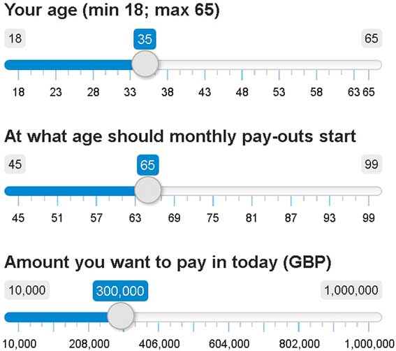
Figure 1 The customer prespecifies some points for the pension product. The age is used to determine the mortality rate.
Figure 2a shows the slider Emma can use in order to see the trade-off between the length of guarantee and monthly benefit size. All amounts are in real terms, i.e. in today’s values, subject to future increases with inflation. This facilitates communication as the amount can be compared with today’s purchasing power. Emma can choose between no guarantee, mimicking a classical financial product or a life-long guarantee, mimicking a deferred annuity and hence no exposure to risk. The accompanying percentage states the chance of ending up with the worst-case scenario of hitting rock bottom zero pension once the guaranteed pension income period is over.
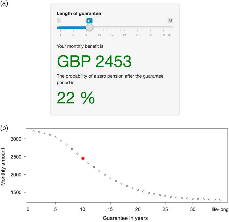
Figure 2 The top figure shows how the customer can choose the length of guarantee via a slider. This then determines the size of the monthly benefit and the probability of a zero pension after the guarantee period. The bottom figure shows the trade-off between guarantee and monthly benefit. In our example, Emma chose a guarantee of 10 years that yielded a monthly real income of £2,453 after retirement.
Imagine that Emma chooses a guarantee period of 10 years providing her a monthly real income of £2,453 until at least the age of 75. If investments go well, with a 50% chance, the monthly payments of £2,453 will continue life long. However, there is also the worst-case scenario, with a probability of 22%, that Emma’s pension income will run out when she reaches 75 years of age. In the remaining 28% case, Emma’s life-long annuity will continue with payouts lower than the targeted £2,453. One could imagine that Emma would safeguard herself to minimise the consequences of such an unfortunate investment performance. She could, for example, incorporate the value of her house when reaching 75 years of age, or buy a second product, perhaps a smaller annuity starting when she is 75 – but then with a life-long guarantee. The annuity option in this paper could be considered as a building block in a more diverse financial planning of the particular household economy Emma faces. It is beyond the scope of this research to illustrate how a wide array of annuities could provide a flexible financial tool for individual households’ financial planning.
In Figure 2b, we see the trade-off between length of guarantee and monthly benefit Emma faces. Note that if Emma did not want any guarantee, her most likely pension outcome would exceed £3,000 a year. Alternatively, if Emma wanted absolute lifetime certainty, the guaranteed income would be below £1,500. Emma can gain a lot by taking the risk of not buying a guarantee, and such should be made clear to her via the graph provided. Emma can also discover that by increasing the age at which pay-outs start in Figure 1, a life-long annuity becomes substantially cheaper.
3. Comparison with Traditional-DC Scheme
In this section, we compare the proposed pension product to a typical DC scheme where at retirement the lump sum is converted to an annuity.
3.1. Guaranteed Income
In the DC scheme, the pensioner is exposed to (a) risk from the financial market, i.e. investment performance in nominal terms, (b) inflation risk, i.e. uncertain development of average living cost and (c) mortality risk, i.e. fluctuations of the annuity price at retirement. These three risks make the final pension hard to predict. Financial planning is, therefore, a challenge for most pension savers holding traditional DC schemes. Our proposed pension product has a clearly stated minimum monthly income, expressed in real terms, aiding the financial planning.
3.2. Performance
We highlight two areas where our suggested pension product seems to outperform the classical DC scheme. First, in DC schemes, risky investments cease at retirement, whereas in our product investments stop at the end of the guarantee period. Those extra years of investment provide our pension saver with either a higher average return or a lower risk. This is because our pension saver has more years to diversify the financial investment risk. Second, in our proposed life annuity product, the pension saver receives additional returns equal to the mortality rate. The full transparency of our pooled mortality provides our pension saver with a significant extra life-long return. In a DC scheme, the added mortality return is opaque and hidden, hence it is expected to be on the lower side. Both features of our product are expected to result in a significantly higher final pension, which is the direct financial benefit. More importantly, there is also an indirect benefit stemming from the fact that our pension saver is more likely to pick the financial risk profile sought, see next.
3.3. Communication
In a classical DC scheme, it is necessary to determine the risk preferences of the pension saver. This is usually done indirectly by means of a procedure that is unrelated with the actual pension, raising the chance of miscommunication and investment in assets that do not fit the actual needs. In our proposed product, the pension saver can directly pick the level of risk sought. He can directly see the trade-off between guarantee and monthly benefit and can pick anything between a no-guarantee product with highest monthly pay-out and a deferred annuity which bears no risk but at the same time gives minimal monthly income. He can also buy more than one product, for example a deferred annuity that starts paying out at age 85 as well as a 20-year guarantee starting at 65. Finally, the choice can be changed at any time by either taking (parts) of the money out or changing the guarantee period.
4. Additional Details
4.1. The Customer Reveals His Risk Appetite
In the above example, Emma revealed her risk appetite in much the same way as proposed for the lump sum case in Gerrard et al. (Reference Gerrard, Hiabu, Kyriakou and Nielsen2017, Reference Gerrard, Hiabu, Kyriakou and Nielsen2018). By specifying the required guarantee length, Emma directly specifies her financial risk appetite. A subsequent simple back-calculation provides us with Emma’s optimal investment strategy. We are in the fortunate situation that the single most important financial risk question Emma faces is one that she understands, is directly linked to her pension, and she can give an immediate answer to: she wants 10 years of guarantee. Perhaps, this is due to children finishing education by then, and her willingness to sell her house when she is 75 renting a smaller apartment instead. Selling the house would only be necessary if investment income turned out to be too disadvantageous. This is rather unlikely and Emma may maintain her current lifestyle without having to withdraw further from her assets including her house. From a regulatory perspective, the pension provider selling the annuity has a full record, for future control purposes, of the financial communication: Emma answered the simple question posed to her with a 10-year period of guarantee ending at the age of 75. The one-to-one fit between communication and pension product drastically reduces the burden of recording the financial advice.
4.2. Annuity Principle
The pension system introduced in this paper uses the annuity overlay fund introduced in Bräutigam et al. (Reference Bräutigam, Guillén and Nielsen2017) and motivated by Donnelly et al. (Reference Donnelly, Guillén and Nielsen2013, Reference Donnelly, Guillén and Nielsen2014) and Stamos (Reference Stamos2008). As the authors point out, while the pooled annuity overlay fund includes the word annuity, the concept is quite distinct from that of a standard life annuity. The main difference is that longevity risk is not transferred to an insurer, but is shared, instead, among the members of the pension fund. The result is an annuity that is transparent in its costs and is actuarially fair.
Whenever an individual in the pension fund dies, his wealth is distributed to the survivors in an actuarially fair way, i.e. at every instant the expected gain (gain when someone else dies less loss of wealth if own death occurs) is zero. Given that the pool is large enough (e.g. 1,000, refer to Donnelly et al., Reference Donnelly, Guillén and Nielsen2013, Reference Donnelly, Guillén and Nielsen2014 for how surprisingly small these annuity pools need to be), the mortality gains are given by
 $$\lambda _{i} (t)X_{i} (t){\rm d}t,$$
where X i is the wealth of individual i and λ i (t) the individual’s force of mortality. The relative annuity gains with magnitude λ i (t) coincide with the growth rate of a fairly priced life-long standard annuity, hence longevity risk is automatically hedged. If Emma reaches the optimal investment scenario, which happens most of the times, the payouts will continue life long.
4.3. The Overall Principle of Hedging and the Importance of Technical simplicity
The most important feature of our new class of pension products is the straightforward communication. Another obvious advantage is its simple technical implementation that will help minimising technical errors from actuarial and financial offices. The simplicity will ensure that actuaries and financial experts are on top of things so that a one-to-one fit is achieved between what actuaries and financial experts tell other departments and the board of directors and what these interested agents actually get. The hedging strategy can be expressed in terms of a simple probability that actuaries immediately understand. The optimal investment strategy before introducing risk sharing is given by investing the amount
 $$\mathop{{\mathop{\underbrace{{{\rm 300,000e}^{{rt{\plus}{\int}_0^t \lambda _{i} (s){\rm d}s}} }}}\limits_{}}}\limits_{{{\rm value}\,{\rm of}\,\pounds{\rm 300,}\,{\rm 000}\,{\rm at}\,t}} {\Bbb P}\left( {0\leq \mathop{{\mathop{\underbrace{{X_{i}^{{\asterisk}} (T_{i} ){\plus}{\cal P}_{i} (0){\minus}{\rm 300,000}\left( {\mu {\minus}r} \right)T_{i} }}}\limits_{}}}\limits_{{{\rm terminal}\,{\rm wealth}\,{\rm of}\,{\rm unconstrained}\,{\rm strategy}\,{\rm corrected}\,{\rm by}\,{\rm drift}}} \leq G_{{U_{i} }} (T_{i} )\mid X_{i}^{{\asterisk}} (t)} \right)$$
in the risky fund, where μ is the average mean return on the risky asset, r the average inflation per year, t the time passed since commencement, T
i
the time from commencement until the end of the guarantee period, λ
i
the force of mortality of individual i,
 $$X_{i}^{{\asterisk}} $$
the wealth of individual i following an optimal unconstrained strategy,
$$X_{i}^{{\asterisk}} $$
the wealth of individual i following an optimal unconstrained strategy,
 $${\cal P}_{i} (0)$$
the initial price of the hedge, and
$${\cal P}_{i} (0)$$
the initial price of the hedge, and
 $$G_{{U_{i} }} (T_{i} )$$
the actuarially fair price at T
i
for a life-long annuity; refer to section 6 for further details.
$$G_{{U_{i} }} (T_{i} )$$
the actuarially fair price at T
i
for a life-long annuity; refer to section 6 for further details.
4.4. How Risk is Pooled
In what follows, our pension saver can invest only in an inflation fund or a risky fund. We assume that both have some risk that has to be taken into account in the financial hedge of the underlying long-term target. In Gerrard et al. (Reference Gerrard, Hiabu, Kyriakou and Nielsen2017, Reference Gerrard, Hiabu, Kyriakou and Nielsen2018), it is assumed that a risk-free inflation fund exists at any given time. Here, we relax this assumption and allow some risk involved when hedging inflation. Most of the time this is not a concern as pension savers can adjust their investments and maintain the same level of risk as if the inflation fund were risk-free (see section 4.4). However, in some rare cases individuals want less risk than the safest option. This can be, for example, the case when 100% in the inflation fund still bears too much risk. The individuals can then take advantage of being part of a group. More specifically, the individuals’ lack of risk appetite can be circumvented by transferring risk to the rest of the group with a risk appetite (see section 4.4). Finally, in extremely rare cases the entire group loses its aggregate risk appetite, rendering the inflow of investments with risk appetite necessary. This implies the need for an intermediary whose role is described in section 4.4.
4.4.1. Individual
Once the individual has specified the length of his guarantee period, an optimal financial hedge is back-calculated. The financial hedge is based on a risk-free inflation fund and a risky fund. It implies at every point in time a certain risk appetite and an optimal level of inflation hedge. When considering a risky inflation fund, those levels can be recovered by adjusting the proportions of the investments. This result is obtained by lowering the level of investment in the risky fund until the risk appetite from the financial hedge is achieved. This implies a slight increase of the investment in the risky inflation fund compared to the original investment in the risk-free fund.
4.4.2. Group
In rare cases, the risk appetite of the individual is so small that risk has to be transferred from the individual to the group. The group, then, chooses, as a solidarity of being part of the group, to borrow money at the risk-free inflation rate and include it in its investments. This allows our pension system to work almost frictionless.
4.4.3. Intermediary
In extremely rare cases with insufficient risk appetite in the group to cover the risk in the inflation fund, an intermediary provides capital with risk appetite. Note that the only promise the intermediary makes is to provide risk capital close to the market value. Therefore, it does not cost much to participate. Even so, the intermediary is allowed to charge some administration cost for being the “market maker” to ensure that risk appetite is available at all times and, therefore, ensure the underlying guarantee.
5. The Stochastic Model Underlying the Financial Hedge
In this section, we present the financial model used for the financial hedging. We choose the simplest possible such model for the sake of transparency, noting that this research output is not aiming for optimal financial modelling. While in this paper we are concerned with connecting investment strategies with annuities and achieving a one-to-one communication to the customer, let us for a second assume that we change the underlying financial model. The financial hedge is about the target income and the length of the guarantee. Changing the financial model is expected to only slightly affect the size of the forecasted target income for given guarantees, however the decision of the pension saver remains more or less of the same nature; this approach seems robust under underlying financial model variations. Therefore, we pick the simplest most transparent model comprising a risk-free inflation fund S 0≡1–note that we operate in real terms–and a risky fund S 1 described via
 $${\rm d}S_{1} (t){\equals}\mu S_{1} (t){\rm d}t{\plus}\sigma S_{1} (t){\rm d}W(t),$$
where μ, σ>0, S 1(0)=1 and W is a standard Brownian motion.
Note that the financial model (1) is simpler than the investment universe provided to the pension customer consisting of a risky asset and an inflation fund, where also the latter carries some risk. The risky inflation fund is expected to be constructed in a way that over the long run at least a return of inflation is obtained plus an additional return corresponding to the risk taken in the risky inflation fund. In section 6.5, we will see that a risk transfer can be made from the real investment universe of a risky inflation fund and a more risky fund to the artificial investment universe of a risk-free inflation fund and a risky fund. The transfer simply looks at the risk that the financial hedging strategy suggests and downplays the risky fund a little bit while upgrading the risky inflation fund a little bit. This is done until the pension customer has the same risk-return profile, as suggested by the very simple transparent financial model (1) consisting of an infeasible risk-free inflation fund and a risky asset.
In the example of section 2, we assume
 $$\mu {\equals}0.0337,\sigma {\equals}0.1538,$$
corresponding to 1-year mean returns and standard deviations of 3.43% and 16% for the risky asset (see equations (10) and (11)). The 3.43% return and 16% volatility of the risky asset are from Guillén et al. (Reference Guillén, L. and Nielsen2006), based on the empirical results in the book “Triumph of the optimist” (Dimson et al., Reference Dimson, Marsh and Staunton2002). In order to price a pension product, the pension provider requires an estimate of the mortality rate, λ(t), of the customer. In Figure 1, this is done by asking for customer’s age. In practice, one may consider more covariates aiming to achieve a better estimate, however such is beyond the scope of this paper. For illustration purposes, we choose for simplicity the mortality rates from the National Life Tables, England, for females in the period 2013–2015 Office for National Statistics (2017). By using this data, we implicitly assume no future period effect on the mortality rates. Again, adopting a more realistic model is possible, but not the focus of this paper. Other information the pension provider receives is the amount of money that the customer wants to invest and the time when payouts should start.
To derive a customer-tailored pension product, it is important to communicate correctly the risk appetite of the customer. Following Gerrard et al. (Reference Gerrard, Hiabu, Kyriakou and Nielsen2017, Reference Gerrard, Hiabu, Kyriakou and Nielsen2018), it is possible to describe the risk appetite with only one parameter that the customer understands. This is in contrast to an abstract risk aversion parameter of a utility function which is hard to communicate. In Gerrard et al. (Reference Gerrard, Hiabu, Kyriakou and Nielsen2017, Reference Gerrard, Hiabu, Kyriakou and Nielsen2018), it is shown that, by specifying a minimum amount the pensioner wants to have guaranteed, an optimal investment strategy can be back-calculated, yielding a practically optimal performance specific to the customer’s risk appetite. In section 6.3, we extend this result to the annuity case in which the customer now chooses how long he wants payouts guaranteed. From equation (8), one can then calculate the corresponding size of monthly payouts, so that there is a 50% chance that these continue life long after the guarantee period.
Note that the money paid in should be invested as long as possible. In particular, investments should not stop at retirement, as such would lead to significant losses in expected performance. In our implementation, we choose the investment to last to the end of the guarantee period. A longer investment horizon is not directly possible as it is a priori not known how long the money on the pension account will last. The customer himself is not concerned with these details and only sees Figure 2, visualising the trade-off between guarantee length and monthly benefit size. Once the decision is made, the pension provider is left with an investment strategy due to be implemented.
Whenever an investor in the pension fund dies, his wealth is distributed according to formula (4). The distribution of wealth is actuarially fair, meaning that, given the individual’s mortality rate, the expected gain at every instant is exactly zero. Note that gains occur if others in the fund die and a loss occurs with own death, the full wealth being redistributed. In Proposition 1, we show that in a large pension pool, payouts from it have little volatility and the extra return from entering the annuity scheme is very close to the mortality rate, λ(t).
The theoretical optimal investment strategy is derived in a Black–Scholes world, hence needs to be adjusted to account for model (1). The main idea is that the strategy is adjusted in a way that the calculated optimal risk exposure from the Black–Scholes world is preserved. This is straightforward to do as long as all individuals in the pension fund have enough risk appetite for the adjustment to be feasible, i.e. equation (13) is fulfilled for everyone. If equation (13) is violated for an individual, the risk-sharing principle kicks in: those with sufficient risk appetite in the pension fund offer those who lack risk appetite a risk-free inflation return; refer to section 6.5.1 for more details. The result is that via this risk-sharing principle, everyone maintains the same risk as derived from the Black–Scholes world.
6. The Full Investment Model Including Mortality Risk
In this section, we incorporate mortality in our financial model. While almost any approach to mortality risk can be combined with our new pension design, we have particular preference for the modern risk-sharing approach of Bräutigam et al. (Reference Bräutigam, Guillén and Nielsen2017) as there are no hidden costs in it to the customers that cover each other’s risk almost without any long-term cost. But again, what follows aims to just illustrate that it is possible to provide an easily communicated pension design including mortality risk. Just as our pension design itself may have several variations with similar positive properties, the underlying mortality approach used for the annuity may also take different shapes without compromising on our overall ideas of a simple pension product that is easy to communicate and where the entire investment strategy can be back-calculated from a short conversation with the pension saver. As pointed out in section 5, we will start with two assets: a risk-free inflation bond S 0 and a risky asset S 1. The financial hedging principle is based on this simple model; mortality risk will be incorporated in section 6.2. The real investment universe the pension customer faces has a risky inflation fund rather than a risk-free inflation bond. Therefore, there is some risk transfer adjustment to be done, so that the pension saver can maintain the risk–return relationship that the financial hedging suggests. This is carried out in section 6.5.
6.1. Two Asset Case: Inflation Fund and Risky Fund
Let us first restate our simple transparent financial model used for financial hedging. There are two assets: a risk-free inflation bond, S 0, and a risky asset S 1, described by
 $${\rm d}S_{0} (t){\equals}rS_{0} (t){\rm d}t,\quad {\rm d}S_{1} (t){\equals}\mu S_{1} (t){\rm d}t{\plus}\sigma S_{1} (t){\rm d}W(t),\quad t\geq 0$$
where μ, σ, r>0 and S
0(0)=S
1(0)=1. The only source of randomness is the standard Brownian motion, W, defined on a complete probability space
 $$(\Omega ,{\cal F},{\Bbb P})$$
. The information available to the investor is represented by the filtration
$$(\Omega ,{\cal F},{\Bbb P})$$
. The information available to the investor is represented by the filtration
 $${\cal F}_{t} {\equals}\sigma \{ W(s),s\in0,t]\} \vee{\cal N}({\Bbb P})$$
, where
$${\cal F}_{t} {\equals}\sigma \{ W(s),s\in0,t]\} \vee{\cal N}({\Bbb P})$$
, where
 $${\cal N}({\Bbb P})$$
denotes the collection of all
$${\cal N}({\Bbb P})$$
denotes the collection of all
 $${\Bbb P}$$
-null sets so that the filtration obeys the usual conditions. We denote by X
i
(t) the amount of wealth invested by individual i in the fund at time t, of which π
i
(t) is invested in the risky asset and the remaining in the risk-free asset. There is also a deterministic stream of payments into the fund defined by
$${\Bbb P}$$
-null sets so that the filtration obeys the usual conditions. We denote by X
i
(t) the amount of wealth invested by individual i in the fund at time t, of which π
i
(t) is invested in the risky asset and the remaining in the risk-free asset. There is also a deterministic stream of payments into the fund defined by
 $${\rm d}{\cal C}_{i} (t)$$
over the time interval (t,t + dt). Hence,
$${\rm d}{\cal C}_{i} (t)$$
over the time interval (t,t + dt). Hence,
 $$\eqalignno{ {\rm d}X_{i} (t){\equals} & r\left( {X_{i} (t){\minus}\pi _{i} (t)} \right){\rm d}t{\plus}\left( {\mu {\rm d}t{\plus}\sigma {\rm d}W(t)} \right)\pi _{i} (t){\plus}{\rm d}{\cal C}_{i} (t) \cr {\equals} & X_{i} (t){\rm d}t{\plus}\left( {\theta {\rm d}t{\plus}{\rm d}W(t)} \right)\sigma \pi _{i} (t){\plus}{\rm d}{\cal C}_{i} (t), $$
where θ=(μ−r)/σ is the market price of risk.
6.2. Adding Pooled Mortality Gains
Next, we consider a fixed, deterministic rate of mortality and the risk pooling principle of Bräutigam et al. (Reference Bräutigam, Guillén and Nielsen2017), and explain how actuarially fair mortality gains can be incorporated in our pension system. In this attempt, we make two assumptions:
A1 The mortality rate of the individuals is known, with no extra parameter uncertainty.
A2 The pension fund has an infinite number of individuals.
We denote the mortality rate of individual i by λ
i
(t). Whenever an individual in the pension fund dies, his remaining wealth is distributed to the survivors in the pension fund. We denote by
 $${\cal L}(t)$$
the index set of people alive at time t. The wealth is distributed in an actuarially fair way. Assume that individual j is alive at time t
−. If he dies at time t, then the surviving pension saver i≠j receives
$${\cal L}(t)$$
the index set of people alive at time t. The wealth is distributed in an actuarially fair way. Assume that individual j is alive at time t
−. If he dies at time t, then the surviving pension saver i≠j receives
 $${{\lambda _{i} (t)X_{i} (t)\left[ {1{\plus}A_{i} (t)} \right]} \over {\mathop{\sum}\limits_{l\in{\cal L}(t_{{\minus}} )} \lambda _{l} (t)X_{l} (t)\left[ {1{\plus}A_{l} (t)} \right]}}X_{j} (t)[1{\plus}A_{j} (t)],$$
where A is an adjustment factor implicitly defined by equation (A1) which converges to zero with growing pool size. More precisely, the individual mortality gains at time t, when individual j dies, are given by
 $${\rm d}H_{i} (t){\equals}\left\{ {\matrix{ {{{\lambda _{i} (t)X_{i} (t)\left[ {1{\plus}A_{i} (t)} \right]} \over {\mathop{\sum}\limits_{l\in{\cal L}(t{\minus})} \lambda _{l} (t)X_{l} (t)\left[ {1{\plus}A_{l} (t)} \right]}}X_{i} (t)\left[ {1{\plus}A_{i} (t)} \right],} \hfill & {\:if\;\:i\,\ne\,j} \hfill \cr {{\minus}X_{i} (t),} \hfill & {\:if\;\:i{\equals}j}, \hfill \cr } } \right.$$
where the case i=j is derived as a consequence of the definition of A.
Proposition 1. The expected mortality gain at every instant is given by
 $${\Bbb E}\left[ {{\rm d}H_{i} (t)\mid {\cal F}_{{t_{{\minus}} }} {\rm ,}\,i\,{\rm alive}\,{\rm at}\,t_{{\minus}} } \right]{\equals}0,$$
hence wealth is distributed in an actuarially fair way. In addition, conditional on surviving, the expected mortality gain is given by
 $$\eqalignno{ {\Bbb E}\left[ {{\rm d}H_{i} (t)\mid {\cal F}_{{t_{{\minus}} }} {\rm ,}\;i\,{\rm alive}\,{\rm at}\,t} \right]{\equals} & \lambda _{i} (t)X_{i} (t)\left[ {1{\plus}A_{i} (t)} \right] \cr& {\times} \left( {1{\minus}{{\lambda _{i} (t)X_{i} (t)\left[ {1{\plus}A_{i} (t)} \right]} \over {\mathop{\sum}\limits_{l\in{\cal L}(t_{{\minus}} )} \lambda _{l} (t)X_{l} (t)\left[ {1{\plus}A_{l} (t)} \right]}}} \right){\rm d}t, $$
and the variance by
 $$\eqalignno{ {\Bbb V}ar\left[ {{\rm d}H_{i} (t)\mid {\cal F}_{{t_{{\minus}} }} {\rm ,}\;i\,{\rm alive}\,{\rm at}\,t} \right] & {\equals} \left( {{{\lambda _{i} (t)X_{i} (t)\left[ {1{\plus}A_{i} (t)} \right]} \over {\mathop{\sum}\limits_{l\in{\cal L}(t_{{\minus}} )} \lambda _{l} (t)X_{l} (t)\left[ {1{\plus}A_{l} (t)} \right]}}} \right)^{2} \cr& \hskip12.5pt {\times} \mathop{\sum}\limits_{j\in{\cal L}(t_{{\minus}} )\,\backslash\,i} X_{j}^{2} (t)\left[ {1{\plus}A_{j} (t)} \right]^{2} \lambda _{j} (t){\rm d}t. $$
Then, with growing pool size, the variance of the actuarial gains converges to zero and the expected gains, conditional on not dying, to λ i (t)X i (t)dt.
Proof. See Appendix A. ∎
In the following, we assume that the pool size is large enough so that any noise can be ignored. Then, if the financial model (3) of the previous section is combined with the annuity pool, as long as the individual is alive the development of wealth is given by
 $${\rm d}X_{i} (t){\equals}\left( {rX_{i} (t){\plus}(\mu {\minus}r)\pi _{i} (t){\plus}\lambda _{i} (t)X_{i} (t)} \right){\rm d}t{\plus}\sigma \pi _{i} (t){\rm d}W(t){\plus}{\rm d}{\cal C}_{i} (t).$$
This means that when an optimal strategy π i is considered, such should incorporate the additional gains λ i (t)X i (t)dt.
Proposition 2. Under model (5), the optimal strategy maximising U(X
i
(T
i
)) for an exponential utility function,
 $$U(x){\equals}{\minus}\gamma _{i}^{{{\minus}1}} {\rm e}^{{{\minus}\gamma _{i} x}} $$
, is given by
$$U(x){\equals}{\minus}\gamma _{i}^{{{\minus}1}} {\rm e}^{{{\minus}\gamma _{i} x}} $$
, is given by
 $$\pi _{i}^{{\asterisk}} (t){\equals}C_{i} {\rm e}^{{{\minus}r(T_{i} {\minus}t){\minus}{\int}_t^{T_{i} } \lambda _{i} (s){\rm d}s}} ,$$
where C i =θ/(σγ i ). Under this strategy, the evolution of the optimal wealth is given by
 $$X_{i}^{{\asterisk}} (t){\equals}{\rm e}^{{rt{\plus}{\int}_0^t \lambda _{i} (s){\rm d}s}} \left[ {X_{i} (0){\plus}g_{i} (0)} \right]{\plus}{\rm e}^{{{\minus}r(T_{i} {\minus}t){\minus}{\int}_t^{T_{i} } \lambda _{i} (s){\rm d}s}} R_{i} \left[ {\theta t{\plus}W(t)} \right]{\minus}g_{i} (t),$$
where
 $$g_{i} (t){\equals}{\int}_t^{T_{i} } {\rm e}^{{{\minus}r(s{\minus}t){\minus}{\int}_t^s \lambda _{i} (u){\rm d}u}} {\rm d}{\cal C}_{i} (s)$$
and R i =C i σ.
Proof. See Appendix B.∎
Remark. Following Gerrard et al. (Reference Gerrard, Hiabu, Kyriakou and Nielsen2017, Reference Gerrard, Hiabu, Kyriakou and Nielsen2018), we assume that
 $$\gamma _{i} {\equals}\theta {\rm e}^{{{\minus}rT_{i} {\minus}{\int}_0^{T_{i} } \lambda _{i} (s){\rm d}s}} \,/\,(\sigma X_{i} (0))$$
so that
$$\gamma _{i} {\equals}\theta {\rm e}^{{{\minus}rT_{i} {\minus}{\int}_0^{T_{i} } \lambda _{i} (s){\rm d}s}} \,/\,(\sigma X_{i} (0))$$
so that
 $$C_{i} {\equals}X_{i} (0){\rm e}^{{rT_{i} {\plus}{\int}_0^{T_{i} } \lambda _{i} (s){\rm d}s}} $$
.
$$C_{i} {\equals}X_{i} (0){\rm e}^{{rT_{i} {\plus}{\int}_0^{T_{i} } \lambda _{i} (s){\rm d}s}} $$
.
6.3. From Lump Sum to Annuities
When considering a retirement product, the focus should not be on a lump sum but on the monthly income level at retirement and the duration of payment. In this section, we extend the lump sum case to an annuity.
Assume that the pension saver has
 $$T_{i}^{0} $$
years until retirement. Assume that individual i chooses to have guaranteed payout duration of D
i
years with payouts of
$$T_{i}^{0} $$
years until retirement. Assume that individual i chooses to have guaranteed payout duration of D
i
years with payouts of
 $${\minus}d{\cal C}_{i} $$
. Payouts stop, however, at the time of death. We set
$${\minus}d{\cal C}_{i} $$
. Payouts stop, however, at the time of death. We set
 $$T_{i} {\equals}T_{i}^{0} {\plus}D_{i} $$
. Then, the discounted remaining guaranteed amount of payments as at t>0 is given by
$$T_{i} {\equals}T_{i}^{0} {\plus}D_{i} $$
. Then, the discounted remaining guaranteed amount of payments as at t>0 is given by
 $$G_{L} _{i}^{{\asterisk}} (t){\equals}{\minus}{\int}_{T_{i}^{0} \vee t}^{T_{i} } {\rm e}^{{{\minus}r(s{\minus}t)}} N_{i} (s)d{\cal C}_{i} (s),$$
where N i has value 1 while the individual is alive, otherwise it becomes 0. We also consider the optimal outcome to be a life-long payout, hence we define the top value based on receipt of payments until death
 $$G_{U} _{i}^{{\asterisk}} (t){\equals}{\minus}{\int}_{T_{i}^{0} \vee t}^\infty {\rm e}^{{{\minus}r(s{\minus}t)}} N_{i} (s)d{\cal C}_{i} (s).$$
Then, t years from now,
 $$G_{{Li}} (t)\,\colon{\equals}{\Bbb E}[G_{L} _{i}^{{\asterisk}} (t)\mid {\cal F}_{t} ]{\equals}{\minus}{\int}_{T_{i}^{0} \vee t}^{T_{i} } {\rm e}^{{{\minus}r(s{\minus}t)}} {{{\cal S}_{i} (s)} \over {{\cal S}_{i} (t)}}d{\cal C}_{i} (s),$$
where
 $${\cal S}_{i} (a){\equals}\exp \left( {{\minus}{\int}_0^a \lambda _{i} (u){\rm d}u} \right)$$
is the survival function, i.e. the unconditional probability of surviving until a certain age, and
$${\cal S}_{i} (a){\equals}\exp \left( {{\minus}{\int}_0^a \lambda _{i} (u){\rm d}u} \right)$$
is the survival function, i.e. the unconditional probability of surviving until a certain age, and
 $$G_{U} _{i} (t)\,\colon{\equals}{\Bbb E}[G_{U} _{i}^{{\asterisk}} (t)\mid {\cal F}_{t} ]{\equals}{\minus}{\int}_{T_{i}^{0} \vee t}^\infty {\rm e}^{{{\minus}r(s{\minus}t)}} {{{\cal S}_{i} (s)} \over {{\cal S}_{i} (t)}}d{\cal C}_{i} (s).$$
Note that
 $$\eqalignno{ & G_{{Li}} (t){\equals}{\minus}g_{i} (t){\plus}{\int}_t^{T_{i}^{0} \vee t} {\rm e}^{{{\minus}r(s{\minus}t){\minus}{\int}_t^s \lambda _{i} (u){\rm d}u}} d{\cal C}_{i} (s), \cr & G_{{Ui}} (t){\equals}{\rm e}^{{{\minus}r(T_{i} {\minus}t){\minus}{\int}_t^{T_{i} } \lambda _{i} (s){\rm d}s}} G_{{Ui}} (T_{i} ){\minus}g_{i} (t){\plus}{\int}_t^{T_{i}^{0} \vee t} {\rm e}^{{{\minus}r(s{\minus}t){\minus}{\int}_t^s \lambda _{i} (u){\rm d}u}} d{\cal C}_{i} (s). $$
We can now modify the unconstrained strategy of the previous section. The aim is to guarantee the payment stream for a period of D i years, while maximising the chance of getting the payouts life long. Technically, this translates to finding an optimal strategy maximising U(X i (T i )), for a given utility function U, subject to the constraint 0=G Li (T i )≤X i (T i )≤G Ui (T i ). Note that the optimal strategy will then naturally satisfy that, at any given time, the wealth remains always above the price of an annuity with D i years payout and below a life-long annuity.
Proposition 3. For
 $$G_{{L} _{i}} (0)\leq X_{i} (0){\plus}{\int}_t^{T_{i}^{0} \vee t} {\rm e}^{{{\minus}r(s{\minus}t){\minus}{\int}_t^s \lambda _{i} (u){\rm d}u}} d{\cal C}_{i} (s)\leq G_{{Ui}} (0),$$
there exists an optimal strategy yielding wealth
 $$X_{i}^{{{\asterisk}{\asterisk}}} (t)$$
with
$$X_{i}^{{{\asterisk}{\asterisk}}} (t)$$
with
 $$X_{i}^{{{\asterisk}{\asterisk}}} (T_{i} ){\equals}\left\{ {\matrix{ {G_{{L_{i} }} (T_{i} ),} \hfill & {{\rm if}\;\:X_{i}^{{\asterisk}} (T_{i} ){\plus}{\cal P}_{i} (0)\,\lt\,0} \hfill \cr {X_{i}^{{\asterisk}} (T_{i} ){\plus}{\cal P}_{i} (0),} \hfill & {{\rm if}\;\:0\leq X_{i}^{{\asterisk}} (T_{i} ){\plus}{\cal P}_{i} (0)\leq G_{{U_{i} }} (T_{i} )} \hfill \cr {G_{{U_{i} }} (T_{i} ),} \hfill & {{\rm if}\;\:X_{i}^{{\asterisk}} (T_{i} ){\plus}{\cal P}_{i} (0)\,\gt\,G_{{U_{i} }} (T_{i} )} \hfill \cr } } \right..$$
Furthermore, it holds for all t ∈ (0, T i ] that
 $$G_{{L_{i} }} (t)\leq X_{i}^{{{\asterisk}{\asterisk}}} (t){\plus}{\int}_t^{T_{i}^{0} \vee t} {\rm e}^{{{\minus}r(s{\minus}t){\minus}{\int}_t^s \lambda _{i} (u){\rm d}u}} d{\cal C}_{i} (s)\leq G_{{U_{i} }} (t).$$
The corresponding optimal strategy is given by
 $$\pi _{i}^{{{\asterisk}{\asterisk}}} (t){\equals}C_{i} {\rm e}^{{{\minus}r(T_{i} {\minus}t){\minus}{\int}_t^{T_{i} } \lambda _{i} (s){\rm d}s}} {\Bbb P}\left[ {G_{{L_{i} }} (T_{i} )\leq X_{i}^{{\asterisk}} (T_{i} ){\plus}{\cal P}_{i} (0){\minus}R_{i} \theta T_{i} \leq G_{{U_{i} }} (T_{i} )\mid X_{i}^{{\asterisk}} (t)} \right],$$
where
 $${\cal P}_{i} (0)$$
is defined via
$${\cal P}_{i} (0)$$
is defined via
 $$\eqalignno{ X_{i} (0) {&\equals} &G_{{U_{i} }} (0){\minus}X_{i} (0)\sigma \sqrt {T_{i} } \left[ {H\left( {{{G_{{U_{i} }} (0){\minus}X_{i} (0){\minus}{\rm e}^{{{\minus}rT_{i} {\minus}{\int}_0^{T_{i} } \lambda _{i} (s){\rm d}s}} {\cal P}_{i} (0)} \over {X_{i} (0)\sigma \sqrt {T_{i} } }}} \right)} \right. \cr & \left. {{\minus} H\left( {{{G_{{L_{i} }} (0){\minus}X_{i} (0){\minus}{\rm e}^{{{\minus}rT_{i} {\minus}{\int}_0^{T_{i} } \lambda _{i} (s){\rm d}s}} {\cal P}_{i} (0)} \over {X_{i} (0)\sigma \sqrt {T_{i} } }}} \right)} \right], $$
 $$H(x){\equals}x \Phi (x){\plus}\phi (x)$$
, and Φ and
$$H(x){\equals}x \Phi (x){\plus}\phi (x)$$
, and Φ and
 $$\phi$$
are, respectively, the standard normal cumulative distribution and density functions.
$$\phi$$
are, respectively, the standard normal cumulative distribution and density functions.
Proof. See Appendix C. ∎
6.4. The Probabilities
In this section, we want to find the monthly payment stream
 $$d{\cal C}_{i} $$
corresponding to monthly constant real income. More specifically, we define
$$d{\cal C}_{i} $$
corresponding to monthly constant real income. More specifically, we define
 $${\cal C}_{i} (t){\equals}{\minus}\mathop{\sum} {\limits}_{s \equals 1}^{12t} M_{i} {\rm e}^{{rs\,/\,12}} $$
,
$${\cal C}_{i} (t){\equals}{\minus}\mathop{\sum} {\limits}_{s \equals 1}^{12t} M_{i} {\rm e}^{{rs\,/\,12}} $$
,
 $$t\,\gt\,T_{i}^{0} $$
and aim to find M
i
, i.e. the monthly income measured in today’s purchasing power, such that
$$t\,\gt\,T_{i}^{0} $$
and aim to find M
i
, i.e. the monthly income measured in today’s purchasing power, such that
 $${\Bbb P}\left[ {X_{i}^{{{\asterisk}{\asterisk}}} (T_{i}^{D} )\,\gt\,0\mid T_{i}^{D} \,\gt\,T_{i} } \right]{\equals}50\,\%\,,$$
where
 $$T_{i}^{D} $$
is the time until death, i.e. given that individual i outlives the guarantee period, there is a 50% chance that the payment stream will continue life long. Assuming independence of the time of death and the performance of the investments, we have that
$$T_{i}^{D} $$
is the time until death, i.e. given that individual i outlives the guarantee period, there is a 50% chance that the payment stream will continue life long. Assuming independence of the time of death and the performance of the investments, we have that
 $$\eqalignno{ {\Bbb P}[X_{i}^{{{\asterisk}{\asterisk}}} (T_{i}^{D} )\,\gt \, 0\mid T_{i}^{D} \,\gt\,T_{i} ]{\equals} & {\int}_{T_{i} }^\infty {{f_{i} (t)} \over {{\cal S}_{i} (T_{i} )}}{\Bbb P}[X_{i}^{{{\asterisk}{\asterisk}}} (t)\,\gt\,0]{\rm d}t \cr {\equals} & {\int}_{T_{i} }^\infty {{f_{i} (t)} \over {{\cal S}_{i} (T_{i} )}}{\Bbb P}\left[ {X_{i}^{{{\asterisk}{\asterisk}}} (T_{i} )\,\gt\,{\minus}{\int}_{T_{i} }^t {\rm e}^{{{\minus}r(s{\minus}T_{i} ){\minus}{\int}_{T_{i} }^s \lambda _{i} (u)du}} d{\cal C}_{i} (s)} \right]{\rm d}t \cr {\equals} & {\int}_{T_{i} }^\infty {{f_{i} (t)} \over {{\cal S}_{i} (T_{i} )}}{\Bbb P}\left[ {X_{i}^{{{\asterisk}{\asterisk}}} (T_{i} )\,\gt\,M_{i} {\rm e}^{{rT_{i} }} \mathop{\sum}\limits_{s{\equals}12T_{i} }^{12t} {\rm e}^{{{\minus}{\int}_{T_{i} }^{s\,/\,12} \lambda _{i} (u)du}} } \right]{\rm d}t $$
where
 $$f_{i} (t){\equals}\lambda _{i} (t)\exp \left( {{\minus}{\int}_0^t \lambda _{i} (s){\rm d}s} \right)$$
is the mortality density. Define
$$f_{i} (t){\equals}\lambda _{i} (t)\exp \left( {{\minus}{\int}_0^t \lambda _{i} (s){\rm d}s} \right)$$
is the mortality density. Define
 $$P_{i} (0){\equals}{\rm e}^{{rT_{i} {\plus}{\int}_0^{T_{i} } \lambda _{i} (s){\rm d}s}} [X_{i} (0){\plus}g_{i} (0)]{\plus}{\cal P}_{i} (0)$$
, then, in distribution,
$$P_{i} (0){\equals}{\rm e}^{{rT_{i} {\plus}{\int}_0^{T_{i} } \lambda _{i} (s){\rm d}s}} [X_{i} (0){\plus}g_{i} (0)]{\plus}{\cal P}_{i} (0)$$
, then, in distribution,
 $$\hskip80pt X_{i}^{{{\asterisk}{\asterisk}}} (T_{i} ){\equals}\max \left\{ {\min \left[ {P_{i} (0){\plus}R_{i} \theta T_{i} {\plus}R_{i} \sqrt {T_{i} } Z,G_{{U_{i} }} (T_{i} )} \right],G_{{L_{i} }} (T_{i} )} \right\}, $$
where Z is a standard normal random variable. Hence,
 $$0.5{\equals}{\int}_{T_{i} }^\infty {{f_{i} (t)} \over {{\cal S}_{i} (T_{i} )}}\Phi \left[ {{{{\minus}M_{i} {\rm e}^{{rT_{i} }} \mathop{\sum}\limits_{s{\equals}12T_{i} }^{12t} {\rm e}^{{{\minus}{\int}_{T_{i} }^{s\,/\,12} \lambda _{i} (u)du}} {\plus}R_{i} \theta T_{i} {\plus}P_{i} (0)} \over {R_{i} \sqrt {T_{i} } }}} \right]{\rm d}t.$$
If
 $${\cal C}_{i} (t){\equals}0$$
for
$${\cal C}_{i} (t){\equals}0$$
for
 $$t\,\lt\,T_{i}^{0} $$
, the above can be rewritten to
$$t\,\lt\,T_{i}^{0} $$
, the above can be rewritten to
 $$\eqalignno{ 0.5{\equals} & {\int}_{T_{i} }^\infty {{f_{i} (t)} \over {{\cal S}_{i} (T_{i} )}}\Phi \left[ {{{{\minus}M_{i} {\rm e}^{{rT_{i} }} \mathop{\sum}\limits_{s{\equals}12T_{i}^{0} }^{12t} {\rm e}^{{{\minus}{\int}_{T_{i} }^{s\,/\,12} \lambda _{i} (u){\rm d}u}} {\plus}R_{i} \theta T_{i} {\plus}{\rm e}^{{rT_{i} {\plus}{\int}_0^{T_{i} } \lambda _{i} (s){\rm d}s}} X_{i} (0){\plus}{\cal P}_{i} (0)} \over {R_{i} \sqrt {T_{i} } }}} \right]{\rm d}t \cr {\equals} & {\int}_{T_{i} }^\infty {{f_{i} (t)} \over {{\cal S}_{i} (T_{i} )}}\Phi \left[ {{{{\minus}M_{i} \mathop{\sum}\limits_{s{\equals}12T_{i}^{0} }^{12t} {\rm e}^{{{\minus}{\int}_0^{s\,/\,12} \lambda _{i} (u){\rm d}u}} {\plus}X_{i} (0)(\mu {\minus}r)T_{i} {\plus}X_{i} (0){\plus}\widetilde{{\cal P}}_{i} (0)} \over {X_{i} (0)\sigma \sqrt {T_{i} } }}} \right]{\rm d}t, $$
where for the last equality we have used that
 $$R_{i} {\equals}X_{i} (0){\rm e}^{{rT_{i} {\plus}{\int}_0^{T_{i} } \lambda _{i} (s){\rm d}s}} \sigma $$
, with
$$R_{i} {\equals}X_{i} (0){\rm e}^{{rT_{i} {\plus}{\int}_0^{T_{i} } \lambda _{i} (s){\rm d}s}} \sigma $$
, with
 $$\widetilde{{{\cal P}_{i} }}(0){\equals}{\rm e}^{{{\minus}rT_{i} {\minus}{\int}_0^{T_{i} } \lambda _{i} (s){\rm d}s}} {\cal P}_{i} (0)$$
– the cost of the hedge when assuming zero inflation. The last equation can be solved iteratively for M
i
. Note that M
i
does not depend on the inflation rate r directly but only via the excess return μ−r.
$$\widetilde{{{\cal P}_{i} }}(0){\equals}{\rm e}^{{{\minus}rT_{i} {\minus}{\int}_0^{T_{i} } \lambda _{i} (s){\rm d}s}} {\cal P}_{i} (0)$$
– the cost of the hedge when assuming zero inflation. The last equation can be solved iteratively for M
i
. Note that M
i
does not depend on the inflation rate r directly but only via the excess return μ−r.
6.5. No Risk-Free Asset but an Inflation Fund
We now relax the assumption of a risk-free asset of the previous section. The reason is that nearly risk-free assets, like bonds, provide a certain nominal return, but a pensioner is more interested in a return with respect to his purchasing power at retirement. By subtracting the inflation rate from an investment return, one derives the real return which, however, bears some risk.
Abandoning the original risk-free asset S 0, we consider now the two assets
 $$d\widetilde{S}_{0} (t){\equals}\widetilde{\mu }\widetilde{S}_{0} (t){\rm d}t{\plus}\widetilde{\sigma }\widetilde{S}_{0} (t)d\widetilde{W}(t),\quad dS_{1} (t){\equals}\mu S_{1} (t){\rm d}t{\plus}\sigma S_{1} (t)dW(t),$$
where
 $$\mu ,\,\widetilde{\mu },\,\sigma ,\,\widetilde{\sigma }\,\gt\,0$$
,
$$\mu ,\,\widetilde{\mu },\,\sigma ,\,\widetilde{\sigma }\,\gt\,0$$
,
 $$\widetilde{S}_{0} (0){\equals}S_{1} (0){\equals}1$$
and
$$\widetilde{S}_{0} (0){\equals}S_{1} (0){\equals}1$$
and
 $$\left( {\widetilde{W},W} \right)$$
is a standard two-dimensional Brownian motion; the correlation coefficient of the Brownian motions is ρ∈[−1,1].
$$\left( {\widetilde{W},W} \right)$$
is a standard two-dimensional Brownian motion; the correlation coefficient of the Brownian motions is ρ∈[−1,1].
6.5.1. Adjusting for extra risk in the inflation fund and the risk sharing principle
To account for the change from the risk-free bond model (2) to the inflation fund (9), we propose an ad hoc adjustment to the optimal strategy (7).
The mean return, μ 1, and risk, σ 1, on £1 in S 1 are given by
 $$\mu _{1} {\equals}{\Bbb E}\left[ {(S_{1} (1){\minus}S_{1} (0))\,/\,S_{1} (0)} \right]{\equals}{\rm e}^{\mu } {\minus}1,$$
 $$\sigma _{1} {\equals}\sqrt {{\Bbb V}ar(S_{1} (1))} {\equals}\sqrt {({\rm e}^{{\sigma ^{2} }} {\minus}1){\rm e}^{{2\mu }} } .$$
In the same fashion for the case when £1 is invested solely in
 $$\widetilde{S}_{0} $$
, we derive μ
0 and σ
0 by replacing μ, σ in equations (10) and (11) with
$$\widetilde{S}_{0} $$
, we derive μ
0 and σ
0 by replacing μ, σ in equations (10) and (11) with
 $$\widetilde{\mu }$$
,
$$\widetilde{\mu }$$
,
 $$\widetilde{\sigma }$$
. For the risk-free case, i.e. when investing in S
0 and S
1, the yearly risk for an individual investing π in S
1 is πσ
1. When we replace the risk-free fund S
0 by the inflation fund
$$\widetilde{\sigma }$$
. For the risk-free case, i.e. when investing in S
0 and S
1, the yearly risk for an individual investing π in S
1 is πσ
1. When we replace the risk-free fund S
0 by the inflation fund
 $$\widetilde{S}_{0} $$
, additional risk (and return) needs to be considered. For wealth X and π invested in S
1, the remaining X−π is invested in
$$\widetilde{S}_{0} $$
, additional risk (and return) needs to be considered. For wealth X and π invested in S
1, the remaining X−π is invested in
 $$\widetilde{S}_{0} $$
and the yearly risk is given by
$$\widetilde{S}_{0} $$
and the yearly risk is given by
 $$\left( {\pi ^{2} \sigma _{1}^{2} {\plus}\left( {X{\minus}\pi } \right)^{2} \sigma _{0}^{2} {\plus}2\pi \left( {X{\minus}\pi } \right)\rho \sigma _{0} \sigma _{1} } \right)^{{1\,/\,2}} .$$
Hence, the risk of individual i is preserved by investing π with
 $$\pi ^{2} \left( {\sigma _{1}^{2} {\plus}\sigma _{0}^{2} {\minus}2\rho \sigma _{1} \sigma _{0} } \right){\plus}\pi \left( {{\minus}2X_{i} \sigma _{0}^{2} {\plus}2X_{i} \rho \sigma _{1} \sigma _{0} } \right){\plus}X_{i}^{2} \sigma _{0}^{2} {\minus}\pi _{i}^{{{\asterisk}{\asterisk}}} ^{2} \sigma _{1}^{2} {\equals}0.$$
The solution
 $$\pi {\equals}{{X_{i} \sigma _{0}^{2} {\minus}X_{i} \rho \sigma _{1} \sigma _{0} {\plus}\left[ {(X_{i} \sigma _{0}^{2} {\minus}X_{i} \rho \sigma _{1} \sigma _{0} )^{2} {\minus}(\sigma _{1}^{2} {\plus}\sigma _{0}^{2} {\minus}2\rho \sigma _{1} \sigma _{0} )(X_{i}^{2} \sigma _{0}^{2} {\minus}\pi _{i}^{{{\asterisk}{\asterisk}2}} \sigma _{1}^{2} )} \right]^{{1\,/\,2}} } \over {\sigma _{1}^{2} {\plus}\sigma _{0}^{2} {\minus}2\rho \sigma _{1} \sigma _{0} }}$$
is well-defined for sufficiently large
 $$\pi _{i}^{{{\asterisk}{\asterisk}}} $$
:
$$\pi _{i}^{{{\asterisk}{\asterisk}}} $$
:
 $$\pi _{i}^{{{\asterisk}{\asterisk}}} \geq X_{i} \sigma _{0} \sqrt {{{1{\minus}\rho ^{2} } \over {\sigma _{1}^{2} {\plus}\sigma _{0}^{2} {\minus}2\rho \sigma _{1} \sigma _{0} }}} .$$
Condition (13) is violated if the individual does not have enough risk appetite, i.e. the optimal strategy involves less risk than any combination of
 $$\widetilde{S}_{0} $$
and S
1 can offer. This leads to the risk sharing principle. More specifically, we arrange the people in the pension fund into three groups. Individuals in groups I and J are those with sufficient risk appetite so that equation (13) holds – see later. Individuals in group K are those with insufficient risk appetite and given the opportunity to invest in the risk-free asset S
0 instead of the risky inflation fund
$$\widetilde{S}_{0} $$
and S
1 can offer. This leads to the risk sharing principle. More specifically, we arrange the people in the pension fund into three groups. Individuals in groups I and J are those with sufficient risk appetite so that equation (13) holds – see later. Individuals in group K are those with insufficient risk appetite and given the opportunity to invest in the risk-free asset S
0 instead of the risky inflation fund
 $$\widetilde{S}_{0} $$
. In turn, the inflation fund
$$\widetilde{S}_{0} $$
. In turn, the inflation fund
 $$\widetilde{S}_{0} $$
replaces S
1 as the risky fund. By slight abuse of notation, we denote by
$$\widetilde{S}_{0} $$
replaces S
1 as the risky fund. By slight abuse of notation, we denote by
 $$\pi _{k}^{{{\asterisk}{\asterisk}{\asterisk}}} $$
, for members of group k∈K, the amount invested in
$$\pi _{k}^{{{\asterisk}{\asterisk}{\asterisk}}} $$
, for members of group k∈K, the amount invested in
 $$\widetilde{S}_{0} $$
, whereas the remaining is invested in S
0. Strategy
$$\widetilde{S}_{0} $$
, whereas the remaining is invested in S
0. Strategy
 $$\pi _{k}^{{{\asterisk}{\asterisk}{\asterisk}}} $$
is adjusted via the risk-preserving relationship
$$\pi _{k}^{{{\asterisk}{\asterisk}{\asterisk}}} $$
is adjusted via the risk-preserving relationship
 $$\pi _{k}^{{{\asterisk}{\asterisk}}} \sigma _{1} {\equals}\pi _{k}^{{{\asterisk}{\asterisk}{\asterisk}}} \sigma _{0} .$$
Note that a solution
 $$\pi _{k}^{{{\asterisk}{\asterisk}{\asterisk}}} \in\left[ {0,X_{k} } \right]$$
exists as the members of group K violate condition (13), hence
$$\pi _{k}^{{{\asterisk}{\asterisk}{\asterisk}}} \in\left[ {0,X_{k} } \right]$$
exists as the members of group K violate condition (13), hence
 $$\pi _{k}^{{{\asterisk}{\asterisk}}} \leq \sigma _{0} X_{k} \,/\,\sigma _{1} $$
.
$$\pi _{k}^{{{\asterisk}{\asterisk}}} \leq \sigma _{0} X_{k} \,/\,\sigma _{1} $$
.
For the strategy to be feasible, the fund S
0 needs to be created internally in the pension fund. This means that those in group I and J have to short S
0 with the amount required by group K. The aggregate amount that needs to be borrowed by members of I and J is
 $$\chi {\equals}\mathop{\sum}\limits_{k\in K} X_{k} {\minus}\pi _{k}^{{{\asterisk}{\asterisk}{\asterisk}}} $$
. The maximum amount individual i∈(I∪J) is willing to borrow is
$$\chi {\equals}\mathop{\sum}\limits_{k\in K} X_{k} {\minus}\pi _{k}^{{{\asterisk}{\asterisk}{\asterisk}}} $$
. The maximum amount individual i∈(I∪J) is willing to borrow is
 $$\xi _{i} {\equals}{{\pi _{i}^{{{\asterisk}{\asterisk}}} } \over {\sigma _{0} \sqrt {{{1{\minus}\rho ^{2} } \over {\sigma _{1}^{2} {\plus}\sigma _{0}^{2} {\minus}2\rho \sigma _{1} \sigma _{0} }}} }}{\minus}X_{i} .$$
The members of group J do not have enough risk appetite for a full support. The subgroups of J are defined iteratively, starting with
 $$J_{1} {\equals}\left\{ {j\in K^{{\complement}} \,\colon\,\xi _{j} \,\lt\,{{\pi _{j}^{{{\asterisk}{\asterisk}}} } \over {\mathop{\sum}\limits_{l\in K^{{\complement}}} \pi _{l}^{{{\asterisk}{\asterisk}}} }}\chi } \right\}\,\subset\,J.$$
If J 1 is empty, the iteration terminates. Otherwise by the mth iteration, the subgroup J m ⊂J is created:
 $$J_{m} {\equals}\left\{ {j\in(K{\cup}J_{1} \cdots {\cup}J_{{m{\minus}1}} )^{{\complement}} \,\colon\,\xi _{j} \,\lt\,{{\pi _{j}^{{{\asterisk}{\asterisk}}} } \over {\mathop{\sum}\limits_{l\in(K{\cup}J_{1} \cdots {\cup}J_{{m{\minus}1}} )^{{\complement}} } \pi _{l}^{{{\asterisk}{\asterisk}}} }}\left( {\chi {\minus}\mathop{\sum}\limits_{l\in(K{\cup}J_{1} \cdots {\cup}J_{{m{\minus}1}} )} \xi _{l} } \right)} \right\}.$$
The iteration stops once an empty set is created. We then define J=∪
l
J
l
. All remaining members of the pension fund are allocated to group
 $$I{\equals}(J{\cup}K)^{{\complement}} $$
. The final strategies for members of I and J are as follows:
$$I{\equals}(J{\cup}K)^{{\complement}} $$
. The final strategies for members of I and J are as follows:
 $$\pi _{l}^{{{\asterisk}{\asterisk}{\asterisk}}} $$
in S
1, −q
l
in S
0 and the remaining in
$$\pi _{l}^{{{\asterisk}{\asterisk}{\asterisk}}} $$
in S
1, −q
l
in S
0 and the remaining in
 $$\widetilde{S}_{0} $$
; q
l
=ξ
l
for members of J, whereas
$$\widetilde{S}_{0} $$
; q
l
=ξ
l
for members of J, whereas
 $$q_{l} {\equals}\left( {\pi _{l}^{{{\asterisk}{\asterisk}}} \,/\,\mathop{\sum}\limits_{i\in I} \pi _{i}^{{{\asterisk}{\asterisk}}} } \right)\left( {\chi {\minus}\mathop{\sum}\limits_{l\in(K{\cup}J)} \xi _{l} } \right)$$
for members of I. Finally,
$$q_{l} {\equals}\left( {\pi _{l}^{{{\asterisk}{\asterisk}}} \,/\,\mathop{\sum}\limits_{i\in I} \pi _{i}^{{{\asterisk}{\asterisk}}} } \right)\left( {\chi {\minus}\mathop{\sum}\limits_{l\in(K{\cup}J)} \xi _{l} } \right)$$
for members of I. Finally,
 $$\pi _{l}^{{{\asterisk}{\asterisk}{\asterisk}}} $$
satisfies (12) when X
l
is replaced by X
l
+ q
l
.
$$\pi _{l}^{{{\asterisk}{\asterisk}{\asterisk}}} $$
satisfies (12) when X
l
is replaced by X
l
+ q
l
.
Acknowledgements
This work was supported by the Institute and Faculty of Actuaries in the UK through the grant “Minimising Longevity and Investment Risk while Optimising Future Pension Plans.”
Appendix A. Proof of Proposition 1
The death of an individual is modelled by a counting process N i (s) with value 1 indicating that the individual is alive. By definition, the counting process has intensity
 $$\mathop {\lim }\limits_{h\downarrow0} h^{{{\minus}1}} {\Bbb E}\left[ {N_{i} \left( {(t{\plus}h)_{{\minus}} } \right){\minus}N_{i} (t_{{\minus}} )\mid {\cal F}_{{t_{{\minus}} }} } \right]{\equals}\lambda _{i} (t){\bf 1}_{{\{ i\,{\rm alive}\,{\rm at}\,t_{{\minus}} \} }} .$$
Hence,
 $$\eqalignno{ H_{i} (t){\equals} & {\minus}\mathop{\sum}\limits_j {\int}_0^t {{\lambda _{i} (s)X_{i} (s)\left[ {1{\plus}A_{i} (s)} \right]N_{i} (s_{{\minus}} )} \over {\mathop{\sum}\limits_l \lambda _{l} (s)X_{l} (s)\left[ {1{\plus}A_{l} (s)} \right]N_{l} (s_{{\minus}} )}}X_{j} (s)\left[ {1{\plus}A_{j} (s)} \right]dN_{j} (s) \cr &{\plus} {\int}_0^t X_{i} (s)\left[ {1{\plus}A_{i} (s)} \right]dN_{i} (s), $$
where A j satisfies
 $$A_{j} (t){\equals}{{\lambda _{j} (t)X_{j} (t)\left[ {1{\plus}A_{j} (t)} \right]} \over {\mathop{\sum} {\limits}_{l} \lambda _{l} (t)X_{l} (t)N_{l} (t_{{\minus}} )\left[ {1{\plus}A_{l} (t)} \right]{\minus}\lambda _{j} (t)X_{j} (t)N_{j} (t_{{\minus}} )}},$$
which can be solved iteratively. Feasibility of this strategy is ensured as
 $$\mathop{\sum}\limits_i H_{i} (t){\equals}0$$
. Furthermore, if individual j dies at time t,
$$\mathop{\sum}\limits_i H_{i} (t){\equals}0$$
. Furthermore, if individual j dies at time t,
 $$dH_{j} (t){\equals}{{\lambda _{j} (t)X_{j} (t)[1{\plus}A_{j} (t)]} \over {\mathop{\sum} \limits_l \lambda _{l} (t)X_{l} (t)\left[ {1{\plus}A_{l} (t)} \right]N_{l} (t_{{\minus}} )}}X_{j} (t)[1{\plus}A_{j} (t)]{\minus}X_{j} (t)[1{\plus}A_{j} (t)]{\equals}{\minus}X_{j} ,$$
where the last equality follows from equation (A1). The expected growth of the gains dH i at time t given that i is alive at t − is given by
 $$\eqalignno{ {\Bbb E}\left[ {dH_{i} (t)\mid {\cal F}_{{t_{{\minus}} }} ,N_{i} (t_{{\minus}} ){\equals}1} \right]{\equals} & {{\lambda _{i} (t)X_{i} (t)\left[ {1{\plus}A_{i} (t)} \right]\mathop{\sum}\limits_{j\in{\cal L}(t_{{\minus}} )} \lambda _{j} (t)X_{j} (t)\left[ {1{\plus}A_{j} (t)} \right]{\rm d}t} \over {\mathop{\sum}\limits_{l\in{\cal L}(t_{{\minus}} )} \lambda _{l} (t)X_{l} (t)\left[ {1{\plus}A_{l} (t)} \right]}} \cr& {\minus} \lambda _{i} (t)X_{i} (t)\left[ {1{\plus}A_{i} (t)} \right]{\rm d}t \cr {\equals} & 0, $$
hence the mortality pooling is actuarially fair at any time. Similarly,
 $$\eqalignno{ {\Bbb E}\left[ {dH_{i} (t)\mid {\cal F}_{{t_{{\minus}} }} ,N_{i} (t){\equals}1} \right]{\equals} & {{\lambda _{i} (t)X_{i} (t)\left[ {1{\plus}A_{i} (t)} \right]\mathop{\sum}\limits_{j\in{\cal L}(t_{{\minus}} )\,\backslash\,i} \lambda _{j} (t)X_{j} (t)\left[ {1{\plus}A_{j} (t)} \right]{\rm d}t} \over {\mathop{\sum}\limits_{l\in{\cal L}(t_{{\minus}} )} \lambda _{l} (t)X_{l} (t)\left[ {1{\plus}A_{l} (t)} \right]}} \cr {\equals} & \lambda _{i} (t)X_{i} (t)\left[ {1{\plus}A_{i} (t)} \right]\left( {1{\minus}{{\lambda _{i} (t)X_{i} (t)\left[ {1{\plus}A_{i} (t)} \right]} \over {\mathop{\sum}\limits_{l\in{\cal L}(t_{{\minus}} )} \lambda _{l} (t)X_{l} (t)\left[ {1{\plus}A_{l} (t)} \right]}}} \right){\rm d}t. $$
For the variance we have
 $$\eqalignno{ {\Bbb V}ar\left[ {dH_{i} (t)\mid{\cal F}_{{t_{{\minus}} }} ,N_{i} (t){\equals}1} \right]& {\equals} \left( {{{\lambda _{i} (t)X_{i} (t)\left[ {1{\plus}A_{i} (t)} \right]} \over {\mathop{\sum}\limits_{l\in{\cal L}(t_{{\minus}} )} \lambda _{l} (t)X_{l} (t)\left[ {1{\plus}A_{l} (t)} \right]}}} \right)^{2} \cr & \quad {\times} \mathop{\sum}\limits_j {\Bbb V}ar[X_{j} (t)\left( {1{\plus}A_{j} (t)} \right)dN_{i} (t)\mid {\cal F}_{{t_{{\minus}} }} ,N_{i} (t){\equals}1] \cr & {\equals} \left( {{{\lambda _{i} (t)X_{i} (t)\left[ {1{\plus}A_{i} (t)} \right]} \over {\mathop{\sum}\limits_{l\in{\cal L}(t_{{\minus}} )} \lambda _{l} (t)X_{l} (t)\left[ {1{\plus}A_{l} (t)} \right]}}} \right)^{2} \cr & \quad{\times} \mathop{\sum}\limits_{j\in{\cal L}(t_{{\minus}} )\,\backslash\,i} X_{j}^{2} (t)\left[ {1{\plus}A_{j} (t)} \right]^{2} \lambda _{j} (t){\rm d}t. $$
Appendix B. Proof of Proposition 2
For notational convenience, in what follows subscript i is suppressed. Define the discounted wealth process
 $$Y(t){\equals}{\rm e}^{{r(T{\minus}t){\plus}{\int}_t^T \lambda (s){\rm d}s}} \left( {X(t){\plus}g(t)} \right).$$
As Y(T)=X(T), maximising
 $${\Bbb E}$$
[U(X(T))] amounts to maximising
$${\Bbb E}$$
[U(X(T))] amounts to maximising
 $${\Bbb E}$$
[U(Y(T))]. Furthermore,
$${\Bbb E}$$
[U(Y(T))]. Furthermore,
 $$dY(t){\equals}(\mu {\minus}r){\rm e}^{{r(T{\minus}t){\plus}{\int}_t^T \lambda (s){\rm d}s}} \pi (t){\rm d}t{\plus}\sigma {\rm e}^{{r(T{\minus}t){\plus}{\int}_t^T \lambda (s){\rm d}s}} \pi (t)dW(t).$$
Based on standard optimal control theory, the optimal value function at time t is given by
 $$\hskip80pt V(t,y){\equals}\mathop {\sup }\limits_\pi \,{\Bbb E}[U(Y(T))\mid Y(t){\equals}y{\rm ,}\,{\rm strategy}\,\pi \,{\rm is}\,{\rm used}].$$
The Hamilton Jacobi Bellman equation describing the dynamics of V is given by
 $$\mathop {\sup }\limits_\pi \left\{ {V_{t} {\plus}\theta \sigma {\rm e}^{{r(T{\minus}t){\plus}{\int}_t^T \lambda (s){\rm d}s}} \pi (t)V_{y} {\plus}{1 \over 2}\sigma ^{2} \pi ^{2} (t){\rm e}^{{2r(T{\minus}t){\plus}2{\int}_t^T \lambda (s){\rm d}s}} V_{{yy}} } \right\}{\equals}0,$$
where V t , V y and V yy are the partial derivatives with respect to t and y (first and second order). By utilising the first-order condition in the optimisation problem above, the optimal value of π is
 $$\pi ^{{\asterisk}} (t,y){\equals}{\minus}{\theta \over \sigma }{\rm e}^{{{\minus}r(T{\minus}t){\minus}{\int}_t^T \lambda (s){\rm d}s}} {{V_{y} } \over {V_{{yy}} }},$$
hence V satisfies
 $$V_{t} {\minus}{{\theta ^{2} } \over 2}{{V_{y}^{2} } \over {V_{{yy}} }}{\equals}0.$$
Subject to the boundary condition
 $$V(T,y){\equals}{\minus}{1 \over \gamma }{\rm e}^{{{\minus}\gamma y}} ,$$
it is straightforward to show that
 $$V(t,y){\equals}{\minus}{1 \over \gamma }\exp \left( {{\minus}{{\theta ^{2} } \over 2}(T{\minus}t){\minus}\gamma y} \right),$$
yielding the optimal strategy
 $$\pi ^{{\asterisk}} (t,y){\equals}C{\rm e}^{{{\minus}r(T{\minus}t){\minus}{\int}_t^T \lambda (s){\rm d}s}} $$
and
 $$Y^{{\asterisk}} (t){\equals}y_{0} {\plus}C\sigma \left( {\theta t{\plus}W(t)} \right).$$
From equations (B1) and (B3), we then get the optimal wealth equation (6).
Appendix C. Proof of Proposition 3
Lemma. Wealth X ** described in equation (7) is feasible.
Proof. Define the process
 $$P(t){\equals}X^{{\asterisk}} (t){\plus}{\cal P}(0),$$
where X
*(t) satisfies equation (6). Further, define the martingale measure
 $${\Bbb Q}$$
such that W
ℚ(t)=W(t) + θt is a standard Brownian motion. Hence,
$${\Bbb Q}$$
such that W
ℚ(t)=W(t) + θt is a standard Brownian motion. Hence,
 $$P(t){\equals}P(0){\plus}RW^{{\Bbb Q}} (t).$$
Conditional on the history of the process up until time t>0,
 $$P(T){\equals}P(0){\plus}R(W^{{\Bbb Q}} (t){\plus}\sqrt {T{\minus}t} Z),$$
where Z is a standard normal random variable under
 $${\Bbb Q}$$
. We note that
$${\Bbb Q}$$
. We note that
 $$P(T)\,\gt\,G_{U} (T)\Leftrightarrow W^{{\Bbb Q}} (t){\plus}\sqrt {T{\minus}t} Z\,\gt\,R^{{{\minus}1}} \left( {G_{U} (T){\minus}P(0)} \right)\Leftrightarrow Z\,\gt\,d_{U} ,$$
where
 $$d_{U} {\equals}{1 \over {\sqrt {T{\minus}t} }}\left[ {R^{{{\minus}1}} \left( {G_{U} (T){\minus}P(0)} \right){\minus}W^{{\Bbb Q}} (t)} \right]$$
and, similarly, we have that P(T)<G L (T) is in distribution equivalent to Z<d L with
 $$d_{L} {\equals}{1 \over {\sqrt {T{\minus}t} }}\left[ {R^{{{\minus}1}} \left( {G_{L} (T){\minus}P(0)} \right){\minus}W^{{\Bbb Q}} (t)} \right].$$
The price of Y
**(T)=X
**(T) at time t is given by the present value of wealth at time t under
 $${\Bbb Q}$$
:
$${\Bbb Q}$$
:
 $$\eqalignno{ Y^{{{\asterisk}{\asterisk}}} (t){\equals} & {\Bbb E}_{{\Bbb Q}} \left[ {\left. {\max \left( {G_{L} (T),\min \left( {G_{U} (T),P(T)} \right)} \right)} \right|{\cal F}_{t}^{{\Bbb Q}} } \right] \cr {\equals} & {\int}_{{\minus}\infty}^{d_{L} } G_{L} (T)\phi (z){\rm d}z{\plus}{\int}_{d_{U} }^\infty G_{U} (T)\phi (z){\rm d}z{\plus}{\int}_{d_{L} }^{d_{U} } \left( {P(0){\plus}R(W^{{\Bbb Q}} (t){\plus}\sqrt {T{\minus}t} z)} \right)\phi (z){\rm d}z \cr {\equals} & G_{L} (T)\Phi (d_{L} ){\plus}G_{U} (T)\left[ {1{\minus}\Phi (d_{U} )} \right]{\plus}\left( {P(0){\plus}RW^{{\Bbb Q}} (t)} \right)\left[ {\Phi (d_{U} ){\minus}\Phi (d_{L} )} \right] \cr& {\minus} R\sqrt {T{\minus}t} \left[ {\phi (d_{U} ){\minus}\phi (d_{L} )} \right] \cr {\equals} & G_{U} (T){\minus}R\sqrt {T{\minus}t} \left[ {H(d_{U} ){\minus}H(d_{L} )} \right]. $$
As H ’(x)=Φ(x)∈(0,1) and d L <d U , we deduce that
 $$0\leq H(d_{U} ){\minus}H(d_{L} )\leq d_{U} {\minus}d_{L} {\equals}{1 \over {\sqrt {T{\minus}t} }}R^{{{\minus}1}} (G_{U} (T){\minus}G_{L} (T)).$$
Returning to the standard measure ℙ, we can write both d L and d U as functions of t and w=W(t):
 $$\eqalignno{ & d_{L} (t,w){\equals}{1 \over {\sqrt {T{\minus}t} }}\left[ {R^{{{\minus}1}} \left( {G_{L} (T){\minus}P(0)} \right){\minus}w{\minus}\theta t} \right], \cr & d_{U} (t,w){\equals}{1 \over {\sqrt {T{\minus}t} }}\left[ {R^{{{\minus}1}} \left( {G_{U} (T){\minus}P(0)} \right){\minus}w{\minus}\theta t} \right], $$
with
 $${{\partial d_{L} } \over {\partial t}}{\equals}{\minus}{\theta \over {\sqrt {T{\minus}t} }}{\plus}{{d_{L} } \over {2(T{\minus}t)}},\quad {{\partial d_{L} } \over {\partial w}}{\equals}{\minus}{1 \over {\sqrt {T{\minus}t} }},$$
and similarly for d U . By exploiting the expressions for d L and d U , we rewrite Y **(t)=η(t,W(t)), where η satisfies
 $$\eqalignno{ {{\partial \eta } \over {\partial t}}& { \equals} {R \over {2\sqrt {T{\minus}t} }}\left[ {H(d_{U} ){\minus}H(d_{L} )} \right]{\minus}R\sqrt {T{\minus}t} \left[ {H^{'} (d_{U} ){{\partial d_{U} } \over {\partial t}}{\minus}H^{'} (d_{L} ){{\partial d_{L} } \over {\partial t}}} \right] \cr& {\equals} {R \over {2\sqrt {T{\minus}t} }}\left[ {H(d_{U} ){\minus}H(d_{L} )} \right] \cr& \hskip8.5pt {\plus} R\theta \left[ {\Phi (d_{U} ){\minus}\Phi (d_{L} )} \right]{\minus}{R \over {2\sqrt {T{\minus}t} }}\left[ {d_{U} \Phi (d_{U} ){\minus}d_{L} \phi (d_{L} )} \right] \cr& {\equals} {R \over {2\sqrt {T{\minus}t} }}\left[ {\phi (d_{U} ){\minus}\phi (d_{L} )} \right]{\plus}R\theta \left[ {\Phi (d_{U} ){\minus}\Phi (d_{L} )} \right], \cr& \hskip-16pt {{\partial \eta } \over {\partial w}}{\equals}{\minus}R\sqrt {T{\minus}t} \left( {H^{'} (d_{U} ){{\partial d_{U} } \over {\partial w}}{\minus}H^{'} (d_{L} ){{\partial d_{L} } \over {\partial w}}} \right){\equals}R\left[ {\Phi (d_{U} ){\minus}\Phi (d_{L} )} \right], \cr& \hskip-20.5pt {{\partial ^{2} \eta } \over {\partial w^{2} }}{\equals}{\minus}{R \over {\sqrt {T{\minus}t} }}\left[ {\phi (d_{U} ){\minus}\phi (d_{L} )} \right], $$
so that
 $$dY^{{{\asterisk}{\asterisk}}} (t){\equals}\left( {{{\partial \eta } \over {\partial t}}{\plus}{1 \over 2}{{\partial ^{2} \eta } \over {\partial w^{2} }}} \right){\rm d}t{\plus}{{\partial \eta } \over {\partial w}}{\rm d}W(t){\equals}R\left( {\Phi (d_{U} ){\minus}\Phi (d_{L} )} \right)\left( {\theta {\rm d}t{\plus}{\rm d}W(t)} \right).$$
Now equation (B2) states
 $$dY(t){\equals}\sigma {\rm e}^{{r(T{\minus}t){\plus}{\int}_t^T \lambda (s){\rm d}s}} \pi (t)\left( {\theta {\rm d}t{\plus}{\rm d}W(t)} \right),$$
for
 $$Y(t){\equals}{\rm e}^{{r(T{\minus}t){\plus}{\int}_t^T \lambda (s){\rm d}s}} \{ X(t){\plus}g(t)\} $$
, hence Y
**(t) is obtained via the strategy
$$Y(t){\equals}{\rm e}^{{r(T{\minus}t){\plus}{\int}_t^T \lambda (s){\rm d}s}} \{ X(t){\plus}g(t)\} $$
, hence Y
**(t) is obtained via the strategy
 $$\pi ^{{{\asterisk}{\asterisk}}} (t,y){\equals}C{\rm e}^{{r(T{\minus}t){\plus}{\int}_t^T \lambda (s){\rm d}s}} \left( {\Phi (d_{U} ){\minus}\Phi (d_{L} )} \right).$$
We now prove that it is possible to choose P(0) in such a way that the budget constraint X(0)=x 0 is satisfied. The budget constraint is
 $$\eqalignno{ Y(0) & {\equals}\eta (0,0) \cr& {\equals}G_{U} (T){\minus}R\sqrt T \left[ {H\left( {R^{{{\minus}1}} {{G_{U} (T){\minus}P(0)} \over {\sqrt T }}} \right){\minus}H\left( {R^{{{\minus}1}} {{G_{L} (T){\minus}P(0)} \over {\sqrt T }}} \right)} \right] $$
with its derivative with respect to P(0) given by
 $$\Phi \left( {R^{{{\minus}1}} {{G_{U} (T){\minus}P(0)} \over {\sqrt T }}} \right){\minus}\,\Phi \left( {R^{{{\minus}1}} {{G_{L} (T){\minus}P(0)} \over {\sqrt T }}} \right)\,\gt\,0.$$
The smallest and largest possible values are therefore the limits as P(0)→±∞: at the top end,
 $$G_{U} (T){\minus}R\sqrt T \mathop {\lim }\limits_{q\to\infty} {\int}_{R^{{{\minus}1}} (G_{L} (T){\minus}q)\,/\,\sqrt T }^{R^{{{\minus}1}} (G_{U} (T){\minus}q)\,/\,\sqrt T } \Phi (z){\rm d}z{\equals}G_{U} (T),$$
and at the bottom end,
 $$\eqalignno{ & G_{U} (T){\minus}R\sqrt T \mathop {\lim }\limits_{q\to{\minus}\infty} {\int}_{R^{{{\minus}1}} (G_{L} (T){\minus}q)\,/\,\sqrt T }^{R^{{{\minus}1}} (G_{U} (T){\minus}q)\,/\,\sqrt T } \Phi (z){\rm d}z \cr & {\equals}G_{U} (T){\minus}R\sqrt T \left( {{{R^{{{\minus}1}} (G_{U} (T){\minus}q)} \over {\sqrt T }}{\minus}{{R^{{{\minus}1}} (G_{L} (T){\minus}q)} \over {\sqrt T }}} \right){\equals}G_{L} (T), $$
as expected. We conclude that it is always possible to find a value of P(0) such that the budget constraint is satisfied as long as
 $$G_{L} (T)\,\lt\,Y(0)\,\lt\,G_{U} (T).$$
Assuming that this inequality holds, we have a strategy which is feasible.
It is left to show that
 $$G_{L} (t)\leq X^{{{\asterisk}{\asterisk}}} (t)\leq G_{U} (t).$$
As
 $$Y^{{{\asterisk}{\asterisk}}} (t){\equals}{\Bbb E}_{{\Bbb Q}} \left( {\left. {\max \left( {G_{L} (T),\min \left( {G_{U} (T),P(T)} \right)} \right)} \right|{\cal F}_{t}^{{\Bbb Q}} } \right),$$
we have that G L (T)≤Y **(t)≤G U (T), and conclude that
 $${\rm e}^{{{\minus}r(T{\minus}t){\minus}{\int}_t^T \lambda (s){\rm d}s}} G_{L} (T){\minus}g(t)\leq X^{{{\asterisk}{\asterisk}}} (t)\leq {\rm e}^{{{\minus}r(T{\minus}t){\minus}{\int}_t^T \lambda (s){\rm d}s}} G_{U} (T){\minus}g(t).$$
We now prove that X ** is optimal.
Let V 0(t, y) be the value function of the proposed solution:
 $$V_{0} (t,y){\equals}{\Bbb E}\left( {{\minus}{1 \over \gamma }{\rm e}^{{{\minus}\gamma Y(T)}} \mid Y(t){\equals}y} \right).$$
We demonstrate the optimality of π** by demonstrating that V 0 satisfies the Hamilton–Jacobi–Bellman equation and that π** is the strategy which gives rise to Y(t). We are faced with the problem that Y(t) is only defined as a function of W(t) and t. We therefore write
 $$V_{0} \left( {t,Y(t)} \right){\equals}V_{0} \left( {t,\eta \left( {t,W(t)} \right)} \right){\equals}\bar{V}\left( {t,W(t)} \right),$$
so that
 $${{\partial \bar{V}} \over {\partial t}}{\equals}{{\partial V_{0} } \over {\partial t}}{\plus}{{\partial V_{0} } \over {\partial y}}{{\partial \eta } \over {\partial t}},$$
 $${{\partial \bar{V}} \over {\partial w}}{\equals}{{\partial V_{0} } \over {\partial y}}{{\partial \eta } \over {\partial w}},\quad {{\partial ^{2} \bar{V}} \over {\partial w^{2} }}{\equals}{{\partial ^{2} V_{0} } \over {\partial y^{2} }}\left( {{{\partial \eta } \over {\partial w}}} \right)^{2} {\plus}{{\partial V_{0} } \over {\partial y}}{{\partial ^{2} \eta } \over {\partial w^{2} }}.$$
Now
 $$\hskip70pt P(T){\equals}P(0){\plus}R\left( {\theta T{\plus}W(T)} \right)\mathop{{\equals}}\limits^{{\cal D}} P(0){\plus}R\left( {\theta T{\plus}W(t){\plus}\sqrt {T{\minus}t} Z} \right),$$
where Z is a standard normal random variable under the original probability measure ℙ. As a result,
 $$\hskip95pt P(T)\,\gt\,G_{U} (T)\Leftrightarrow Z\,\gt\,D_{U} (t,w)\mathop{{\equals}}\limits^{{def}} d_{U} (t,w){\minus}\theta \sqrt {T{\minus}t} $$
(D L follows similarly from P(T)<G L (T)). Given the previous definition, we get
 $$\eqalignno{ \bar{V}\left( {t,w} \right){\equals} & {\Bbb E}\left( {{\minus}{1 \over \gamma }{\rm e}^{{{\minus}\gamma Y(T)}} \mid W(t){\equals}w} \right) \cr {\equals} & {\minus}{1 \over \gamma }\left( {{\int}_{{\minus}\infty}^{D_{L} } {\rm e}^{{{\minus}\gamma G_{L} (T)}} \phi (z){\rm d}z{\plus}{\int}_{D_{U} }^\infty {\rm e}^{{{\minus}\gamma G_{U} (T)}} \phi (z){\rm d}z} \right. \cr& \left. {{\plus} & {\int}_{D_{L} }^{D_{U} } {\rm e}^{{{\minus}\gamma \left( {P(0){\plus}R(\theta T{\plus}w{\plus}\sqrt {T{\minus}t} z)} \right)}} \phi (z){\rm d}z} \right) \cr {\equals} & {\minus}{1 \over \gamma }\left( {{\rm e}^{{{\minus}\gamma G_{L} (T)}} \Phi (D_{L} ){\plus}{\rm e}^{{{\minus}\gamma G_{U} (T)}} \left( {1{\minus}\Phi (D_{U} )} \right)} \right. \cr& \left. {{\plus} {\rm e}^{{{\minus}\gamma P(0){\minus}{1 \over 2}\theta ^{2} (T{\plus}t){\minus}\theta w}} \left( {\Phi (D_{U} {\plus}\theta \sqrt {T{\minus}t} ){\minus}\Phi (D_{L} {\plus}\theta \sqrt {T{\minus}t} )} \right)} \right), $$
with
 $$\eqalignno{ {{\partial \bar{V}} \over {\partial w}} & {\equals}{\minus}{1 \over \gamma }\left( {{\rm e}^{{{\minus}\gamma G_{U} (T)}} {{\phi (D_{U} )} \over {\sqrt {T{\minus}t} }}{\minus}{\rm e}^{{{\minus}\gamma G_{L} (T)}} {{\phi (D_{L} )} \over {\sqrt {T{\minus}t} }}{\minus}\theta {\rm e}^{{{\minus}\gamma P(0){\minus}{1 \over 2}\theta ^{2} (T{\plus}t){\minus}\theta w}} \left( {\Phi (d_{U} ){\minus}\Phi (d_{L} )} \right)} \right. \cr & \hskip8.7pt\left. {{\minus}{\rm e}^{{{\minus}\gamma P(0){\minus}{1 \over 2}\theta ^{2} (T{\plus}t){\minus}\theta w}} \left( {{{\phi (d_{U} )} \over {\sqrt {T{\minus}t} }}{\minus}{{\phi (d_{L} )} \over {\sqrt {T{\minus}t} }}} \right)} \right). $$
As
 $$\eqalignno{ \phi (D_{U} ){\equals} & {{{\rm e}^{{{\minus}{1 \over 2}d_{U}^{2} {\plus}\theta d_{U} \sqrt {T{\minus}t} {\minus}{1 \over 2}\theta ^{2} (T{\minus}t)}} } \over {\sqrt {2\pi } }}{\equals}\phi (d_{U} ){\rm e}^{{{\minus}{1 \over 2}\theta ^{2} (T{\minus}t){\plus}\gamma G_{U} (T){\minus}\gamma P(0){\minus}\theta w{\minus}\theta ^{2} t}} \cr {\equals} & \phi (d_{U} ){\rm e}^{{\gamma G_{U} (T){\minus}\gamma P(0){\minus}{1 \over 2}\theta ^{2} (T{\plus}t){\minus}\theta w}} $$
(similarly for D L ), we get that
 $${{\partial \bar{V}} \over {\partial w}}{\equals}R{\rm e}^{{{\minus}\gamma P(0){\minus}{1 \over 2}\theta ^{2} (T{\plus}t){\minus}\theta w}} \left( {\Phi (d_{U} ){\minus}\Phi (d_{L} )} \right)$$
and, consequently,
 $${{\partial ^{2} \bar{V}} \over {\partial w^{2} }}{\equals}R{\rm e}^{{{\minus}\gamma P(0){\minus}{1 \over 2}\theta ^{2} (T{\plus}t){\minus}\theta w}} \left( {{\minus}\theta \left( {\Phi (d_{U} ){\minus}\Phi (d_{L} )} \right){\minus}{1 \over {\sqrt {T{\minus}t} }}\left( {\phi (d_{U} ){\minus}\phi (d_{L} )} \right)} \right).$$
Then, from equation (C2),
 $$\eqalignno{ {{\partial V_{0} } \over {\partial y}} & {\equals}{\rm e}^{{{\minus}\gamma P(0){\minus}{1 \over 2}\theta ^{2} (T{\plus}t){\minus}\theta w}} , \cr& {{\partial ^{2} V_{0} } \over {\partial y^{2} }}{\equals}{{{{\partial ^{2} \bar{V}} \over {\partial w^{2} }}{\minus}{{\partial V_{0} } \over {\partial y}}{{\partial ^{2} \eta } \over {\partial w^{2} }}} \over {\left( {{{\partial \eta } \over {\partial w}}} \right)^{2} }}{\equals}{\minus}\gamma {{{\rm e}^{{{\minus}\gamma P(0){\minus}{1 \over 2}\theta ^{2} (T{\plus}t){\minus}\theta w}} } \over {\Phi (d_{U} ){\minus}\Phi (d_{L} )}}, $$
and from equation (C1),
 $$\eqalignno{ {{\partial V_{0} } \over {\partial t}}{\equals} & {\rm e}^{{{\minus}\gamma P(0){\minus}{1 \over 2}\theta ^{2} (T{\plus}t){\minus}\theta w}} \left( {{{R\theta } \over 2}\left( {\Phi (d_{U} ){\minus}\Phi (d_{L} )} \right){\plus}{R \over {2\sqrt {T{\minus}t} }}\left( {\phi (d_{U} ){\minus}\phi (d_{L} )} \right)} \right) \cr& {\minus} {\rm e}^{{{\minus}\gamma P(0){\minus}{1 \over 2}\theta ^{2} (T{\plus}t){\minus}\theta w}} \left( {R\theta \left( {\Phi (d_{U} ){\minus}\Phi (d_{L} )} \right){\plus}{R \over {2\sqrt {T{\minus}t} }}\left( {\phi (d_{U} ){\minus}\phi (d_{L} )} \right)} \right) \cr {\equals} & {\minus}{{R\theta } \over 2}{\rm e}^{{{\minus}\gamma P(0){\minus}{1 \over 2}\theta ^{2} (T{\plus}t){\minus}\theta w}} \left( {\Phi (d_{U} ){\minus}\Phi (d_{L} )} \right), $$
from which
 $${{\partial V_{0} } \over {\partial t}}{\minus}{{\theta ^{2} } \over 2}{{\left( {{{\partial V_{0} } \over {\partial y}}} \right)^{2} } \over {{{\partial ^{2} V_{0} } \over {\partial y^{2} }}}}{\equals}0$$
follows. Hence, the value function satisfies the Hamilton–Jacobi–Bellman equation: we conclude that this must be the optimal strategy.


 Open access