

The Chairman (Mr H. Patel, F.I.A.): This sessional meeting is on improving understanding and transparency around the assessment of inflation and will be presented by members of the IFoA’s Limited Price Indexation (LPI) Risks Working Party.
I am a member of the Finance and Investment Practice Area Board, and we indirectly oversee a number of working parties, including this one. In my day job, I am an Investment Director at Legal and General, supporting its With Profits fund.
I am very pleased to introduce Alexandra (Al) Miles and John Southall. Al is a Senior Solution Strategy Manager at Legal and General Investment Management (LGIM), supporting Defined Benefit and Defined Contribution clients to implement broader solution-based investment strategies. Previously, Al worked on the consultancy side with Willis Towers Watson. Al is the Chair of the LPI Risk Working Party, and she is also the Deputy Chair of the Research Sub Committee of the Finance Investment Practice Area.
John (Southall) is currently the Head of Solutions Research at LGIM and was previously a Senior Investment Strategist Risk Manager. Prior to joining LGIM, John also worked on the consultancy side with Punter Southall. John is also a member of the LPI Risks Working Party.
I am sure everybody will agree that in an age of increasing risk management, risk budgeting, and, ultimately, risk transfer, it is vitally important that we have a common understanding of how we assess, measure, and manage LPI exposures. Just thinking about my own experience as an Investment Strategy Manager, I have found that when trying to hedge this risk, we have often been constrained by our own confidence in the underlying measures, so, as a result, you think that by coming up with too precise a hedge, that there is a risk of spurious accuracy. So, I am really pleased by the work this working party is doing, which will help overcome, hopefully, some of those hurdles and, more importantly, help standardise thinking.
I understand that there are a couple of papers that underpin the presentation that are going through the peer review process.
Ms A. M. A. Miles, F.I.A.: Thank you, Hetal (Patel). I thought I would start by running through the terms of reference for our working party.
There are two main aims of our working party that we set out as our high-level aims. The first aim is to improve understanding, and our second aim is to increase transparency in the area of calculating the inflation sensitivity of LPI-linked liabilities.
In order to do this, we have gathered a wide body of people from across the industry, representing actuaries, investment consultants, asset managers, insurers, and academics. So, there is a wide gathering of people with various different skill sets and experiences to date, which we thought was key to the progress of this LPI risk working party.
In terms of what we look to generate going forward, the first stage was a deep dive audit of all the existing methodologies that people use across the industry when calculating the inflation sensitivity of LPI-linked liabilities. Off the back of that, we are in the progress of putting together some simple worked examples in spreadsheet format, which we will also publish, so people can go in and have a look and play around with the key assumptions, the outputs, and what is driving what for themselves, which I think is key to improving understanding and increasing transparency in this area.
We have two key outputs to which Hetal (Patel) alluded, focused on two different sections of our readership. One is a simple guide or a layman’s guide to this area. Something that a trustee could potentially pick up and have a look at and get to grips with a general understanding of this area, which is, in itself, quite technical. The second output is a detailed academic style paper going through, very thoroughly, the modelling detail. It is something that, maybe, a quant would look at who is already practised in the area. So, we are appealing to both those areas, which we thought was quite important in the output from this working party.
In terms of key industry players, we have five. Pensions actuaries are the closest to the raw data and to the pension scheme. They have two main objectives: setting the valuation assumptions on an ongoing basis and consolidating and publishing the scheme summary information in terms of it being used by other third parties across the industry.
Investment consultants have a primary aim to construct the investment strategy in order to hedge the inflation sensitivity of the LPI-linked liabilities. Obviously, the methodology chosen to calculate that inflation sensitive LPI-linked liability is a key driver to the investment strategy which you select.
The methodology chosen, the calibration technique for that methodology, any key assumptions, as well as the underlying scheme data, can all influence the end picture, and John Southall will go through that in a bit more detail later on.
The two key outputs that we have highlighted from this exercise are usually an IE01 risk data profile for a scheme or a set of fixed and real liabilities. So, that is the split once you have calculated the inflation sensitivity of your LPI-linked liability benchmark and those in themselves are influenced, as I say, by the methodology chosen, calibration technique and the underlying key assumptions.
Key to all of this is transparency, and I think to date maybe there has been a lack of transparency, with lots of players in the market and lots of data available. Maybe some things could be lost in translation. So, part of the output, or part of the aim of this working party, is to make clear the key things that you would need to know when handling that data. Maybe more detail about the underlying data, and not just taking the benchmark at face value, because quite a lot of factors can influence that benchmark.
Next, we have the asset managers. They are implementing the benchmark that has been constructed and designed by the consultant or actuary. They can also become involved in constructing the benchmark, and increasingly, we are seeing asset managers step into that space. They can also take account of trading costs, market liquidity constraints, and LPI swaps on the book held by a pension scheme on the asset side.
They also have a think about the end objective of the exercise, such as whether it is a cashflow-matching approach or a risk-driven approach. That, potentially, can have an influence on the methodology that you choose which, in turn, is driving your benchmark.
Then you have the insurers. There are two main aims for insurers: setting up sufficient reserves and structuring the capital to meet the liabilities. They will be influenced by internal prudence and external regulatory prudence, as well as commerciality, such as whether they are going to win a deal based on the pricing basis that they have chosen.
Key things influencing the methodology they would go for would include cashflow stability of the benchmark, ease of ongoing monitoring of the benchmark, and materiality on the assumptions being made.
The fifth and final set of key players are the trustees. Their main aim is to oversee the scheme, paying the pensions that have been promised to members. They are also interested in the implications on any liability benchmark in terms of the level of contributions required from the employer and the volatility of those employer contributions going forward. They are not technical experts, and they do have a day job themselves, so they rely quite heavily on their advisors to fill the gaps.
In terms of valuing the inflation sensitivity of LPI-linked liabilities, there are four key approaches. The work of the LPI Risk Working Party to date has focused on the delta hedging approach, but, for completeness, we will briefly cover three other approaches.
The simplest of the methodologies is the binary approach. This is where, if inflation is lying above an LPI cap or below the floor, you would assume that LPI-linked benefit is effectively fixed. Then, when inflation is lying between the cap and the floor, you assume that it is 100% inflation linked. There is no middle grey area which you might see with a delta hedging approach.
The main issue with this approach is, perhaps, a cashflow mismatch risk, especially when inflation is sitting at or around the cap or the floor. So this approach is generally used in combination with holding a reserve approach.
The second approach is “holding a reserve” and takes account of the implicit cost, or negative cost, of where inflation is lying, and the mismatch generated between your assets and your liabilities. Assume that you are holding 100% inflation-linked assets against LPI-linked liabilities. If inflation rises above your cap, that is a negative cost. The inflation earned by your assets is more than the inflation you need for your liabilities. The reverse is true if inflation is lying below your floor.
So you run several simulations, or lots of simulations, and calculate a net aggregate cost, and that becomes the inflation reserve that you would hold.
The third approach is an LPI asset approach that, at a high level, looks like it is the ideal solution, but it also has issues. Your ideal hedging instruments are LPI swaps. There is also LPI debt and LPI-linked property infrastructure available. It is quite a limited supply and, as a result, quite expensive for a scheme to buy. Also, it is not so good when trying to match more esoteric LPI-linked increases, for example, LPI(2.5, 7), as opposed to LPI(0, 5).
The fourth and final approach on which we will focus is the delta hedging approach. This is where you would use an option pricing model to calculate the inflation sensitivity of your LPI-linked liabilities and then calculate your inflation-linked assets in order to match that inflation sensitivity calculated on your liabilities. That would go through a regular review and recalibration to check that it stays relatively in line.
What are the reasons for picking a certain approach? There can be short-term or long-term outlooks. Depending on the pension scheme, they might be interested in hedging a short-term balance sheet volatility between valuations, or possibly aligning their approach with a buyout provider. That would mean, or could mean, that they want to align their methodology to be similar to the one chosen by an actuary or a buyout provider.
Cashflow matching or risk matching, we touched on earlier. The binary hedging approach is, possibly, less adequate when looking at a cashflow-matching approach compared with a risk-matching approach.
What is the client trying to achieve? So if a client, for example, is looking to set out a long-term hedging strategy, it is possibly better to hedge the true economic value of LPI, so they might use a real-world model rather than a market-consistent model, and we will go on to the details of that issue later.
Regulatory requirements are applicable. International Financial Reporting Standards (IFRS) stipulates a market-consistent basis, so if you are following IFRS you may be constrained in the approach that you can use.
If you are already holding LPI swaps on your assets, you may want to adopt a consistent approach on your liability as well, which might lead you to adopt a market-consistent approach rather than a real world.
Finally, any requirements to replicate methodologies are similar to the first point around adopting or aligning your methodology with somebody else that you know it is important to align yourself with, whether that be an actuary or a buyout provider.
We now have a quick-fire jargon buster before we go into the details of the modelling. We will set out a few of the key terms that we will be using as we go through the rest of this presentation.
Delta, which has already been covered briefly, is a sensitivity of the present value of your liabilities to changes in underlying inflation. It is usually expressed as a percentage, sitting somewhere between 0% and 100%. So fixed would be 0% and 100% would be Retail Price Index (RPI).
Skew is the difference in implied volatility of an at-the-money option compared to an in-and-out-of-the-money option, and that can be affected by sentiment or market demand (a supply and demand relationship). Giving an example, if you look back at historical inflation, and John will come on to cover this in a bit more detail later, if you had a fairly symmetrical distribution for inflation, you might expect to find limited or no skew in the distribution that you were using to drive your methodology.
Smile, then, is a particular case of skew. So this is where your at-the-money option has a lower implied volatility than in-and-out-of-the-money options. That means your call or put has increasing implied volatility as the strike price moves away from the current market price and can be severely driven by demand.
Autocorrelation is the degree of similarity between a given time series and a lag of itself. So that shows the influence of the past on the future. For example, if you were to look back prior to the inflation-targeting regime which came in during 1992, periods of high inflation would typically be followed by other periods of high inflation, so displaying autocorrelation.
Market consistency is a term we will use a lot in the remainder of our presentation. You have strong, weak, and not market consistent. Strong and weak fully replicate the nominal yield curve and full-term structure of breakeven inflation. Strong market consistency goes that step further and also replicates market prices of zero coupon LPI swaps at various different strike prices.
Finally, real world is moving away from market consistency. It is being driven, primarily, by historic behaviour but then being recalibrated back to current market conditions.
Dr J. O. Southall, F.I.A.: One of the key questions when it comes to managing LPI liabilities is whether you take a market-consistent approach or a real-world approach.
There are various pros and cons involved, and one of the key advantages of a market-consistent approach, or indeed of market-consistent approaches in general, is that it is objective. The trouble with subjective approaches is that it is always very tempting to choose assumptions that give you the answer that you would like. Not that an actuary would ever dream of such a thing.
The other potential advantage of a market-consistent approach is that it is good to have that kind of approach if you execute or hold LPI swaps, or other LPI assets, and that you have greater consistency between your assets and your liabilities, because otherwise your LPI swaps and your LPI liabilities will not move in line with each other, despite the fact that they are perfectly matching assets.
In terms of disadvantages of a market-consistent approach, one of the key disadvantages is that it is arguably becoming increasingly unrealistic. It is becoming increasingly difficult to calibrate models to fit the pricing. A further disadvantage is that the data must be paid for and somebody along the line has to absorb that cost.
The alternative to a market-consistent approach is a real-world approach. The real-world approaches that we have looked at, at least weakly market consistent, as Al previously defined, so they replicate the gilt curve and breakeven inflation. Where they differ is instead of looking at the prices of LPI swaps, they use historic realised inflation to guide how you set your assumptions regarding the distribution of future inflation.
So, a real-world approach sounds like a good way to go given what is happening in the LPI swap market, but there are disadvantages. In particular, there is a lack of data. We only have, for example, gilt yields going back to 1985. Inflation targeting began in 1992, so that gives you relatively limited amount of data on which to base your assumptions. As such, it can be quite unclear how bad some of your simplifying assumptions may be and, obviously, it is a more subjective exercise, which can be dangerous.
There are four main models that we investigated or have started to investigate. There is the Black model, sometimes referred to as the Black–Scholes model. Technically, the model that is used is the Black one, where it is calibrated to forward prices rather than spot prices as an input. It is the simplest model and assumes that there is a log normal distribution for inflation each year and that each year is independent of the previous one. You can fit it to market prices if you want, but a problem with doing that is that you can only fit one strike per term, so it is not very flexible in that regard.
There is the so-called Jarrow-Yildirim (JY) model. This can be thought of as an extension to the Black model. The central idea of this model is that it is based on a foreign currency analogy. You can almost imagine two economies, one nominal economy and one real economy, and the RPI effectively acts like an exchange rate between the two.
You can simplify it, if you put in simplifying parameters and you can recover the Black model. But what you can also do is to model things like stochastic interest rates. You can capture the autocorrelation of inflation that I mentioned earlier. One thing you cannot do is to capture skew under this approach.
There are alternatives. For example, you could use a commercial Economic Scenario Generator (ESG). This could be weak or strong, and this is full bells and whistles, which you can make as fancy as you like. You can have stochastic interest rates, stochastic real rates, pickup autocorrelation and skew. The trouble with it is it is not nearly as transparent. There are no closed-form formulae, so you have to look at simulations. Obviously, that is highly subjective, but that definitely is one option.
Then, we have the Stochastic Alpha Beta Rho (SABR) model. This is, effectively, a very flexible model for fitting to market prices, and it is a very convenient way of doing so because you can generate a lot of different shapes just by tweaking the parameters. However, it is arguably not really very sound as a stochastic model. It does not model inflation in a particularly realistic way. That does not matter under a market-consistent approach because you can always compensate by adjusting your parameters. All you are effectively trying to do is to obtain a nice interpolation and extrapolation of market pricing.
That is why we have not really seriously considered SABR as something you would use for a real-world model.
Let us look now at a couple of more detailed points.
In terms of the autocorrelation point, the idea that if you have high inflation is more likely to be followed by more high inflation than suddenly deflation. One way you can see that is by comparing RPI swap rates with year-on-year swap rates. So, for a year-on-year swap, the floating leg is basically based on the inflation increase in a single year in the future, whereas for an RPI swap, the floating leg is based on cumulative inflation.
What you can do is, you can take your year-on-year rates and you can compound them up, annualise them, and compare them with your RPI swap rates, as in Figure 1.
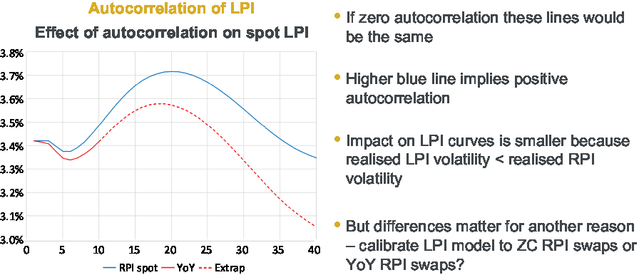
Figure 1. Autocorrelation of LPI.
Now, naively, you might think those sound very similar, so why do they not give the same curves? There is a difference going on in that when you are looking at the RPI spot rates, you are effectively looking at the expectation of a product, whereas when you are taking the product of the year-on-year rate, you are doing a product of expectations.
These two things, an expectation of product and a product of expectations, are not the same thing. You might remember, if you think back to your CT3 or university statistics, the definition of covariance is the expectation of a product, minus the product of an expectation. So that is why we see the blue line, which is the RPI spot rate, exceeding the red line. It is because the market is effectively pricing in the possibility of positive feedback loops that lead to inflation either being stubbornly high or stubbornly low. The market is not completely confident that the Bank of England will necessarily be able to control inflation.
Moving on to another feature: skew. Later on, we will look at the skew implied by market pricing, but in terms of skew that you might want to use in a real-world model, what we have done here is we have just plotted yearly realised inflation since 1992. The reason we chose 1992 was because that is when inflation targeting began. As we can see in Figure 2, realised inflation has been broadly symmetric other than a blip during the financial crisis. It is based on a rolling period, which is why it looks like there are several data points.
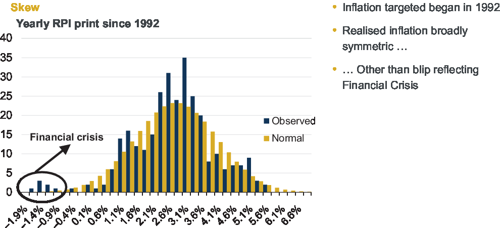
Figure 2. Skew.
Focusing on the real-world models for now, one of the key questions we considered is, how can you calibrate the simplest and most commonly used model, the Black model?
Frequently, when people are calibrating this model, they just look at the volatility of realised inflation, but this is not strictly the right approach. For example, you should really be looking at realised inflation relative to what you expected it to be. For example, if you are looking at a 10-year point, what you might want to do is go 10 years back, look at the breakeven inflation curve and the 10-year point on that, and then compare how inflation behaved over the subsequent 10-year period with what was expected. That is quite important because, when you are building this model, you are building it around the expected inflation curve.
So the question then is, exactly how can we calibrate it? We cannot just literally repeat historic inflation because, obviously, the curves are no longer the same, so we need to scale it in some way to basically replicate current prices.
What we did was to take realised inflation relative to expectations, expressed these as cumulative factors, and scaled them to today’s curves. Then, essentially, what this model does is to look at many rolling periods and calculate what is called a burning cost of the caps and the floors. Then, you back out the volatilities that you would plug in to the Black model to recover those values.
So, that is the essential idea. As you can see on the graph in Figure 3, there is very limited evidence of skew. For this particular example, we have looked at LPI(0, 5). The red line reflects the cap and the green line reflects the floor. There is not statistically much difference between them. The model seems to be implying a volatility assumption of somewhere between 1.5% and 2%.
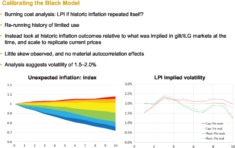
Figure 3. Calibrating the Black model.
This is one of the spreadsheets that we hoped to publish. You could specify different caps, different floors, and this model will back out the implied volatilities that the burning cost analysis suggests that you ought to use. There is also additional functionality in the spreadsheet in that it will calculate your hedging portfolio and things like that, which is potentially useful.
So, in terms of looking at some results, I said for the Black model an inflation volatility assumption of somewhere between 1.5% and 2% looks sensible. We chose 1.8% just to show as an illustration. We had to choose a date as well, so we chose 31 October 2017 because we were able to source some market pricing for LPI swaps at the same date, so later we can do a comparison.
The graphs in Figure 4 show some results in the terms of the value of the cap and the value of the floor, and also the resulting LPI curve, as a result of the calculations.
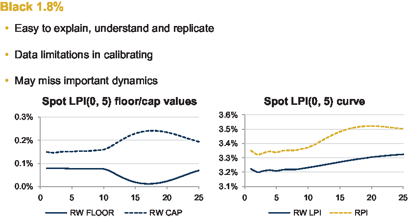
Figure 4. Black 1.8%.
The cap is more valuable here than the floor, and this is simply a function of the fact that at this analysis date, expected inflation is closer to the cap than it is to the floor. It has an interesting bowl shape, like it is a wine glass on its side. Essentially, this just reflects that the RPI curve increases from around 10 to 20 years. So that pushes up the value of the cap and, at the same time, decreases the value of the floor. The key takeaway is that at least for this particular cap and this particular floor, at this date, the LPI curve is lower than the RPI curve for this real-world approach.
The other key approach is the market-consistent approach where, as we have said, you fit parameters to LPI quotes from banks at key tenors, and one of the key advantages is that it is highly flexible in terms of extrapolation and interpolation. So it captures skew and smiles and all sorts of nice shapes. But the problem with the market-consistent approach has been that the number of quotes has reduced and the dispersion between those few quotes that we do get has also increased, so arguably, it is not very realistic. For example, it would not satisfy Active, Deep, Liquid, and Transparent (ADLT) criteria under Solvency II.
We have been saying for a while that it is unrealistic, so as an illustration that it is unrealistic, what we have done on the graph in Figure 5 is we have plotted spot implied volatilities. Just for comparison, we have the Black 1.8%, which is just a flat line at 1.8%. We have plotted the implied volatility for 5% cap, so that is the blue line, and it looks pretty close to fair pricing. Then, we have plotted the floor. This starts off at something that looks sensible or fair, but the implied volatility rapidly increases. In other words, it looks expensive, unless you believe there is a very high chance of deflation in the future. The reason we suspect this is the case is that there is a lot of demand for this floor from pension schemes, but there is very little supply on the other side, it has been very difficult to find a natural supply.

Figure 5. Stochastic Alpha Beta Rho.
I have tried to put this all together in Figure 6.

Figure 6. How much impact does choice of model have?
If you imagine at the moment a scheme with a market-consistent approach, but because of the concerns we have raised they are thinking of moving to a real-world approach. What might the impact be? There are really two considerations. IE01, which is defined as the change in Present Value (PV) from a 1-basis point move in inflation, is driven by two factors. One of these factors is how high or low the LPI curve is, that is fairly clear, and the second point is this delta or percentage type sensitivity.
Now, if you have a scheme that is interested in funding level hedging, it is interesting in that you only care about the delta for the purpose of constructing the hedge, because you are hedging up to the level of the assets. The actual value of the liabilities is not relevant. You are just trying to mirror the same percentage split in terms of fixed and real. But if you are interested in deficit hedging, you obviously do care about how high or low that LPI curve is.
In terms of these two effects, I have shown an example of moving from market consistent to real world. In terms of valuation, the LPI curve is largely above the RPI curve, but the real-world curve is below. When you look at the impact at a typical scheme duration of maybe 20 years, there is about a 30-basis point gap in this particular case, which might be a 6%-ish decrease in the present value of your liabilities.
The story for deltas is in the opposite direction. So because you are moving to something which overall has less volatility, those caps and floors and less likely to apply, in particular the floor is really less likely to apply, so the delta goes up. So in this case, we actually move from 61% to 76% delta, which relatively speaking is a 25% uplift. The impact is the combination of these two, so we have got a 6% decrease, but we have got a 25% increase, with a bit of rounding we get an 18% overall increase in IE01.
I think we will need to expand out our illustrations, consider different caps and floors, maybe look at other dates in terms of what breakeven inflation, but this is the kind of analysis that we are looking into.
At the same time, we are keen to stress that LPI risk obviously is not the whole story. So it is very important that the risk is considered in context. Figure 7 shows estimates of various risks that schemes face.
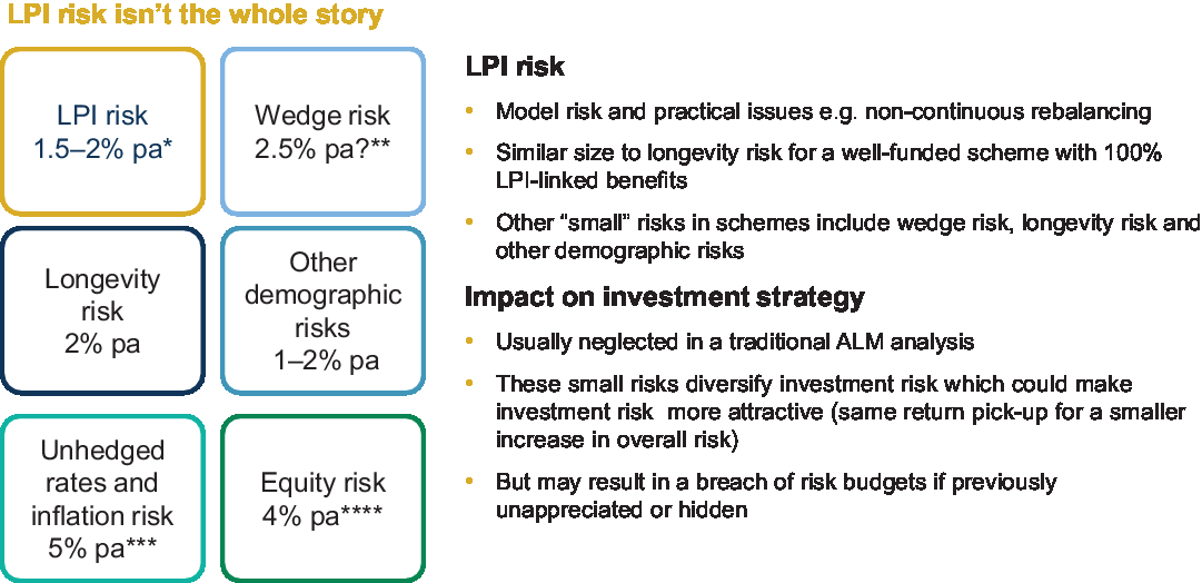
Figure 7. LPI risk is not the full story.
One thing I will comment on is what exactly we mean by LPI and risk, because we have not defined that, even though it has been implicit in what we are saying. LPI risk is the risk, essentially, that your model is wrong. Not that you have made a mistake, but just it is impossible to know exactly what the correct inflation distribution is. If your model is wrong, then you accidentally end up with the wrong delta assumptions and valuation assumptions, so you end up being either under or over exposed to inflation, and therefore, ultimately, there is a risk that your assets are not lined up with your liabilities in terms of meeting cash flows.
This 1.5–2% assumption can become quite messy because, essentially, we are trying to do model on model. I think all parameter uncertainty problems face this issue, but under a simple approach we basically assume there is about a 70% chance that inflation volatility is within 50-basis points of our 1.8% assumption. Then, across many different simulations, calculate how much you are under or over exposed to inflation and then the knock-on impact of that.
It is quite interesting in that the potential risk is quite sizable. These numbers assume that 100% of your liabilities are LPI linked, which obviously is unlikely to be true. You can always scale this number down. It is quite a considerable number, and as schemes de-risk, as they become better funded, I think it is a risk that they are going to increasingly be looking at.
I think our work highlights, in particular with the existence of LPI risk, that many people will not have thought about that very much. It will not be obvious either because, as long as you are doing the same thing on your assets and your liabilities, in the short term, they are going to move in line, and you are not even going to notice anything is happening. Obviously, if you have chosen the wrong model and inflation does not behave as you assumed it would, in the long run you are going to be mismatched.
Recognising this risk does have consequences. For example, you may not want to rebalance quite as frequently as you thought you might because if you do not really know if the inflation volatility assumption you should be using is 1.3 or 2.3, although it might look like you were significantly mismatched, you could still be using a delta hedge that could be justified by a perfectly reasonable model.
Ms Miles: In terms of key takeaways, and then looking to what we plan around some future work and output from this working party, we have taken you through pros and cons of the different approaches and focussed on market-consistent and real-world approaches at a high level. John has looked at a particular example, highlighting the potential impact of using one approach over the other. He talked about the 6% fall in PV and about an 18% increase in IE01 for that particular example. We have also developed a method that will feed into user-enabled spreadsheets that will output from this working party, looking at burning cost analysis and historical data, and using that to calibrate the Black model. We have also covered a range of different data limitations, both in the real world and the market-consistent methodologies. Those exist for any approach undertaken – there is no escaping them.
In terms of our planned future work, we have some further work looking at the JY model. To date, we have focussed more on the Black and the SABR. Then, a bit more guidance to our end users around those key assumptions and the impact of those key assumptions on the end output in terms of the liability benchmarking inflation sensitivity calculated through your LPI-linked liabilities. So, perhaps guidance about the 1.8 key assumption of the implied volatility for the Black model, including how certain we are on that 1.8, maybe giving a flavour of, if you were to change it to 1.5 or 2, what the additional implications would be for that resulting liability benchmark.
Then, there are simple examples of key models and their outputs. These will be in spreadsheet format that everyone can use. We are going to try and make them as simple as possible, so that people can play around and become comfortable with the key assumptions and the various points of calibration.
There is also the production of a simple guide to this area. It is a very technical area, so it would be good to have a simple guide that someone like a trustee can use to get a broad understanding, so that they can challenge their actuary or asset manager and have more debate and conversation around this topic, rather than just taking the assumption as given.
The Chairman: Excellent. With that, I am going to open the debate up for questions.
Mr J. G. Spain, F.I.A.: The idea of transparency being focussed upon actuarial work is really to be applauded, so thank you for that. However, I did spot a couple of things along the way which I thought were not transparent. For example, you said there were five key players. There are not five key players. There are at least six, and that would include the Sponsors, and you do not seem to have thought about the Pension Regulator. They are involved as well.
Second, the pensions actuary does not set the valuation assumptions anymore. They may recommend them, but it is a trustees’ responsibility, and that is quite important.
I obtained the impression along the way that some of the pricing was in the swap space, but it is very difficult to get a lot of data.
I gather from something that Andrew Smith said that you are looking at index-linked gilt against conventional gilts. The trouble is they do not give you a decent result at all. You would probably be much better off looking at the Bank of England yield curves, which are much better at predicting inflation.
Mr M. Ashmore, F.I.A.: Just trying to understand, when you are talking about the Black model, and what you are applying Black to, and particularly the log normal distribution, because my thinking is, and I may have misunderstood, that the log normal model assumes that the variable that has that log normal distribution can only ever be positive, and so if we are trying to model floors, and particularly the floor at zero, how good a choice is the log normal model is for trying to value the floor at zero?
Dr Southall: It is the RPI index, which, you can imagine, if you think of a log normal for a stock price, for example, it is similar to that but instead of the stock price, you are talking about the RPI index. So, each year, if you are expecting inflation at 2%, then each year the RPI increase could be 2%, but it could have volatility around that, so it could be that the RPI falls.
Mr Ashmore: Thank you.
Mr J. A. Fermont, F.I.A.: When you were talking about the SABR model, you were talking about the data that are available to calibrate it, I particularly noted that the number of participants has come down, and so it may not meet the ADLT criteria. Do you have any specific numbers on the number of participants, and also did the working party look into whether those quotes, the data you have, were just indicative marks or were those actual transacted prices?
Ms Miles: In terms of number providers, I think, pre-financial crisis, there were maybe eight or nine regularly providing quotes. That we have seen drop to maybe two or three at key tenors. Maybe that is just one at some of the tenors, so really becoming quite light on data. Those quotes themselves are quite disparate, so it is not like they are all in the same ballpark. They are just quotes, not transactions.
Mr I. W. McKinlay, F.F.A.: I was interested in the risks that you had calculated, and one of them I was quite surprised at was the wedge. Just intuitively, that wedge risk just feels awfully high to me but can you explain exactly what you mean?
Dr Southall: So, by wedge risk, you mean you have Consumer Price Index (CPI)-linked liabilities but you are using RPI-linked assets to try and hedge those. The risk here can be surprisingly large, as you say.
If you look at the correlation between RPI and CPI, both in terms of realised inflation and based on the limited amount of expected inflation that we have, they are quite highly correlated, as you would expect. It is about an 80% correlation.
In addition, RPI and CPI do have similar volatilities, but when you work through the maths you are looking at the volatility of RPI minus CPI. You have the volatility of RPI squared plus the volatility of CPI squared minus twice times 0.8 and so on. You do the square root, and you get a number that is left, that is about 60% of the volatility.
By hedging CPI liabilities with RPI-linked assets, you are left with (it is all approximate) about half the risk still on the table. So, this particular 2.5% number, we are saying, let us suppose, just as an example, the scheme is 50% CPI and you are only using RPI-linked instruments, and if the mark-to-market volatility from inflation risk is about 10% per annum, breakeven inflation volatility is about 50-basis points, and so on, that is how you get to the 2.5% figure. I agree that it is very surprising.
Mr J. S. Neale, F.I.A.: The government is due to respond to the House of Lords RPI survey this month. Would it change the calibration of your numbers if there are significant changes to the RPI index?
Dr Southall: It is definitely something we should take into account. I suppose, in an extreme scenario, the RPI might move to be completely in line with the CPI. So, obviously that would change the initial inflation curve that all the calculations are based on. In terms of volatility, it probably would not change that much, given that CPI and RPI have a slight difference but they have broadly similar volatility. In terms of all the principles that we are applying here, I think that they would remain the same.
Mr G. S. Mee, F.I.A.: When you were looking at calibrating the Black model, were you looking at empirical volatility over the time period that you looked at?
Dr Southall: Yes, what we were doing is essentially looking at realised inflation relative to expected inflation over different periods.
Mr Mee: Normally, if you were pricing an option in the market, then you would have an increase, so the difference between implied volatility and empirical volatility. Did you look at needing to uplift the empirical volatility in your calculations, and if so, did that get you closer to the market-consistent numbers?
Dr Southall: We did not look at uplifting it. We just basically took that realised versus expected, recalibrated it and backed up the vols. So no, we did not allow for any potential uplift.
Mr H. Popat, F.I.A.: In carrying out your research, did you get a sense of which market participants used which types of models, because looking at it from a pension scheme trustee’s perspective, today they might be looking at the scheme actuaries model, which might typically be Black, JY or some variation of that class of models.
At some point, they will probably be looking at what insurers might be interested in, if they are going to go down the buy-out route. If they are in run-off, then they can live forever in scheme actuary world, which may drift as a result of your work, but do you have a sense of where the insurers are and what they are allowed to do by their regulators?
Ms Miles: We did start by doing a broad audit, and the insurers were more likely to follow a market-consistent SABR methodology. Pensions actuaries, as you say, were more likely to use the Black model. Asset managers probably look to use a market-consistent but potentially move more towards aligning themselves with the actuaries going forwards, so potentially allowing clients to use or have the flexibility to adopt a more real-world or Black approach.
Mr R. A. Rae, F.I.A.: I have done a little bit of work on this when we were looking to value income strips on long-lease properties, and we were trying to work out the expected inflation that you might use. I work for an asset-management company, and my colleagues naturally opted for a market-consistent approach but were dogged because there is absolutely no market-consistent data out there in terms of implied volatilities over a term structure.
I can see the problems that you are facing. Have you done any work or are you intending to do any work that might look at current assumptions that are being used on the various approaches, and seeing how you measure it in terms of expected inflation across a term structure or a delta that you would place.
Dr Southall: In assets base, effectively?
Mr Rae: Well, however, you are comparing the different approaches in terms of how material those differences could be based on what you might consider to be a common set of assumptions or perhaps testing their sensitivity.
Dr Southall: Yes, that is one of the key parts. We sort of touched on it a little bit, and then we have compared the market. I compared the market consistent with the real-world approach, and you can see the impact in terms of both the valuation and in terms of the sensitivity to inflation. That is obviously just one example. Obviously, we cannot show every example, but we can show a broader set.
Mr Rae: So you are showing the sense of the material differences there.
Dr Southall: Yes.
Ms Miles: Yes, and in the simple guide, we will highlight the key assumptions, those to focus on that have a material impact on the outcome. In terms of the benchmark, that you end up or the IO1 risk ladder that you end up generating.
Mr Rae: Any comments on actuarial judgement here at this point in time?
Dr Southall: I suppose the nice thing about the real-world approach is there is some scope for actuarial judgement, but obviously there are pros and cons with that. I think it would be nice if we can publish this spreadsheet and it would give a common tool. So, there would probably be less variance in terms of how people choose to set their volatility assumption because often, the way it is done, is, in our view, a little bit oversimplified, and this gives a more robust approach.
The Chairman: Since the early '90s, we have been in this inflation-targeting regime and inflation has been very benign. To what extent have you taken into account data prior to that low inflation environment, and how do you think it would impact your results? Is there an intention of modelling more extreme scenarios in your work going forwards?
Dr Southall: In terms of the burning cost model that we used, we can only go as far back as January 1985, but you are right to say, if you look in the 1970s, for example, there was very high inflation volatility. I think there is always a dilemma in turns of trading off relevance and volume when you are deciding how much data that you use. I think, if we could, going back into the 1970s, we would provide more data, it would arguably be a lot less relevant, given that there is no inflation targeting involved. In terms of the burning cost model, we again set that up with input parameters, so you can sensitivity test it to different starting points and end points. Just testing with that, broadly, you get very similar results over different periods since 1985, which gives some comfort.
Mr L. M. Townley, F.I.A.: In motor insurance, there are periodic payment orders. They are linked to care-worker inflation, and that can be quite volatile. It can be negative some years. It can be double-digits other years. We would quite like to have an LPI cap and collar I think, but those liabilities are very long-tailed. So, you have a minor in a motor accident, and then you could be paying these claims for 60, 70, 80, and 90 years, ultimately. I was just interested in what the pros and cons of some of your methods for really long-tail liabilities and just thinking of last liquid points, are they influenced by ultimate forward rates?
Dr Southall: I think, obviously, the further you are trying to project out, the harder and harder it does become. So, when we did our burning cost analysis, for example, the maximum we went out to was 10 years, so that at least we had a few independent 10-year rolling periods. So, I think when you start looking that far out, you have to just become more and more pragmatic and really extrapolate. If there is a flat-term structure, as far as you can tell, it is obviously sensible, unless you have got a good reason to think otherwise, just to extrapolate that out. Yes, to answer your question, I think looking at the long term just involves actuarial judgement.
Mr K. Washoma, F.I.A.: When can we expect publication of the more detailed paper and the spreadsheet?
Dr Southall: We have not quite decided how much is going to be included in the detailed paper at the moment. So, we may just publish the details behind the burning cost model, together with the spreadsheet at the same time, and I would imagine that could be within the next few months. I think we are largely there but we just need to do due diligence, I suppose.
Mr Washoma: Yes, because without seeing that, there is an element of reading between the lines on how exactly you have treated some of the parameters that you have used in your calibration.
Dr Southall: Yes. Obviously, we cannot go through every bit of detail here.
Mr A. J. Uglow, F.I.A.: Hetal (Patel) mentioned at the start spurious accuracy, and I wondered if you had any thoughts on whether that was something that was a key issue in the LPI space.
Dr Southall: Yes. As I was saying before, I think there is quite a bit of parameter uncertainty just because, when it comes to a real-world model, we do have quite limited data available. So, in particular, and I am not saying you should not use a JY model, I think you should always not make your models more complicated than they need to be. Given that there is little skew that we can tell with historic inflation, there does not seem to be much kurtosis. As I say, there is not that much data or evidence of autocorrelation. So, I think the hurdle, to move away from a Black model, to use something more complicated for a real-world approach, is probably quite high, given that.
Mr Uglow: I wondered if you had any takeaways of what you might hope could help improve understanding in the industry.
Ms Miles: Our two aims were to improve understanding and to increase transparency, and hopefully, when the full report and the spreadsheet come out, we will have gone some way to meeting those two key objectives of the working party.
We are always keen to hear about a different area that we could look into. Obviously, we have just focussed on RPI or Limited Retail Price Index (LRPI) to date, potentially an idea to look into CPI and Limited Consumer Price Index (LCPI), because lots of schemes these days have CPI-linked liabilities. The work of the working party will adapt and be led by what people in the industry would like us to look into in more detail.
Ms Y. T. Loh, F.I.A.: There is a comment that market-consistent approaches, arguably, are realistic, especially on floors. If so, will real world achieve a better hedge over the long term? I am wondering if real world will provide a better hedge over the long term in terms of the actual outcome, inflation outcome, that real-world hedging will provide versus the liabilities. If so, does that happen in all scenarios or only in certain inflation scenarios that you are thinking about?
Dr Southall: Yes, I think those are theoretical ideals. If you knew, with certainty, the way inflation was going to behave, and you were able to continuously rebalance your delta hedge, then, in theory, you would perfectly match your cash flows. That is the justification behind the statement that if inflation distribution as implied by market pricing is unrealistic, in that we do not really think that there is such a high chance of deflation, then if you delta hedge under real-world assumptions, you are not going to perfectly match with cash flow, but it is likely to be closer.
Ms Loh: Yes, so given we have not really had a very sustained period of deflation, I am assuming that if we look back historically, that results will presumably show, at least for the last 20 years, and that real-world hedging will produce better results than model-driven approach or market-consistent approach.
Dr Southall: Yes, almost by construction in terms of the burning cost model, but I agree, it would be good to test that to almost prove the delta hedging point. If you had perfect foresight, so you set the assumptions in line with the Black model that your hedge would have been better. I think that would be a good exercise in illustrating the benefits.
Prof A. D. Wilkie, F.F.A., F.I.A.: I was very interested in learning something about it from your presentation. Some of it takes me back to some work I have done some years ago on hedging. This was just very simple one-way hedging, but the way I, Howard Waters and Mark Owen approached it, one needed a hedging model, a delta hedging approach, to decide on the investment policy but you then needed a real-world model to test it out.
We simulated the real-world model lots of times for lots of years ahead, assuming that you did the delta hedging, and, as you were saying, if you could hedge continuously and costlessly, and you knew the appropriate sigma and you were right about that, then the delta hedging would perfectly match.
As you said, you cannot do that. You do not know the thing, so it helps to do the delta hedging, but one comment early on was, “How accurate might this be?” One thing we found was that this was for ordinary hedging of what I call a maxi option; the higher of share price and some fixed amount, which is the floor side of it. You will get the curve. You will be wholly in cash if the share price was very low and wholly in share if the share price was very high. There was the usual option curve in between.
If you put a straight line through that, so you just had a horizontal, a slope and another horizontal, and tested that within a real-world model, which was different, necessarily, in each simulation from what your assumptions were, you were not much worse off than if you had done, on this crude model, and if you did the delta hedging. That was one point that a good approximation can be really not too bad.
Another obvious point is that as you say, the retail price index cannot possibly do geometric Brownian motion because it is only published monthly. It is not moving continuously anyway, it is a jump process, but what is interesting is the size of the jumps, both monthly and, in the sort of analysis I have done, annually. I have been doing quite a bit more on that recently, putting in stochastic hedging, stochastic interpolation within the yearly model, and looking at the distribution of the jumps. They are very fat-tailed, if you take sufficiently much data (I do not know about limiting it to the most recent years, but obviously it has been more benign in recent years). There is quite a lot of fat-tailed-ness in the monthly jumps, as well as in the yearly ones, and almost more so than in many of the other investment variables that one can look at. So instead of a normal distribution, something like a Laplace or a hyperbolic distribution, which are not terribly well known in this context, but some people use them, fits the past data a lot better.
It is worthwhile also, I think, within a real-world model, since you are only making estimates of the parameters, possibly from a limited amount of past data, if you use maximum likelihood estimation to estimate the values of the parameters within your model, you can also get the standard errors in the correlation coefficients. You can assume that it is multi-variant, normal distribution of the parameters. So, within this simulation, you first of all simulate the values of the parameters for this simulation. Then, as the years go by or months go by, you simulate the outcomes using those parameters. So, you have got what I would call the “hyper model”. I think these are useful ideas but they have not been terribly much talked about or generally in the literature. I think these are areas that can be explored for this purpose.
A problem, in a way, is that the limitation from nought to five is pretty narrow compared with the past history. There have not been big drops in prices in the past, but between 1918 and 1921, I think prices dropped by about 20% a year. There were huge drops in prices and in wages. It was what was known as the Geddes Act. People imagined that the experience in the First World War was that the war-time inflation was temporary. In the Second World War, people assumed that it might also be temporary. On the wages side, people got cost of living increases, which were not pensionable. The basic salary remained the same. At the end of the war, prices did not drop but it was not until several years after the war that salaries were then consolidated, or the cost of living increase was then consolidated to people’s salaries and they started becoming pensionable.
So, the past history of inflation, which goes back an enormously long way, there is data going back to about the 1200s, less relevant than one would expect. I do not think you can avoid subjective, actuarial subjective, judgement in anything you do about it.
How long a period do you look at? You are looking at 20-something years, estimating your parameters. I tend to look at 90 years and estimate the parameters. Other people could certainly, quite comfortably, look at 200 years and estimate the parameters, if there are good data going back that far. If you are looking at quotes on option prices, you get an implied volatility from the market. Then, if you go and measure the data, you get an observed volatility from some past data. Which one do you use? It is a matter of your subjective judgement as to which one you use.
Ms Miles: Thank you very much.
The Chairman: Thank you. There is lots of food for thought there.
Mr Washoma: As a follow-up from that, as a matter of interest, which real-world model did you use for your analysis?
Dr Southall: That was the Black model with 1.8%.
Mr Washoma: I assumed you had used an ESG of some sort.
Dr Southall: No, we deliberately took a simple approach that is quite commonly used, so you could sort of see what might be a fairly typical impact.
Mr Washoma: Did you think to test it against one of the alternatives available that are generally used for doing Asset and Liability Management (ALM) and so on? That would cover some of the points raised around the distributional assumptions.
Dr Southall: We could do but I guess one issue is there are so many different ways you can parameterise it, as I have been saying, there is lots of actuarial judgement involved, so you would have to choose a set of parameters for that. A second issue is in terms of disclosure. We would have to get permission, and even obtaining just the market-consistent data was quite challenging. In terms of the output that the working party can publish, that is a little bit of a hurdle.
Prof Wilkie: The Wilkie Model is a simple ESG that you are free to use.
The Chairman: Thank you very much for that. I think it is safe to say there is a great deal of interest in this area, and so we are all really looking forward to when these additional papers come out.
Our representatives here have made very clear that they want to come up with research that is useful to you. So, I do encourage you to reach out, through the Institute and Faculty of Actuaries (IFoA), to let the working party know any particular direction you would like them to take. Thank you very much to the audience. That was really a healthy debate, lots of challenging questions asked, lots of good feedback, and most of all, our presenters, thank you for the presentation, and sitting through quite a tough cross-examination. Thank you to yourselves and the LPI Risk Working Party.


 Open access