


Introduction
Species distributions are influenced by biotic and abiotic factors, which may operate at different scales and vary between different geographical settings (Guisan and Thuiller Reference Guisan and Thuiller2005, Sirami et al. Reference Sirami, Caplat, Popy, Clamens, Arlettaz, Jiguet and Brotons2017). Therefore, in the context of global change, unravelling the main drivers of species distribution will be useful for land managers and conservation practitioners in developing guidelines aimed at conserving biodiversity (Pullin and Steward Reference Pullin and Stewart2006, Brambilla et al. Reference Brambilla, Gustin, Cento, Ilahiane and Celada2020).
The Mediterranean region is a biodiversity hotspot affected by more frequent droughts and rising temperatures (Lionello and Scarascia Reference Lionello and Scarascia2018) in which rear-edge populations of northern organisms occur despite the effects of increasingly hostile environmental conditions (Hampe and Petit Reference Hampe and Petit2005, Cuttelod et al. Reference Cuttelod, Garcia, Abdul Malak, Temple, Katariya, Vie, Hilton-Taylor and Stuart2008). This suggests that the current distribution of these southern populations may change or vanish in the most vulnerable sectors under climate change (Hampe and Jump Reference Hampe and Jump2011, Merker and Chandler Reference Merker and Chandler2020). This pattern is expected for forest birds, a set of species dependent on woodlands in the core of the western Palaearctic that, according to predictions, will be increasingly scarce in the southernmost ranges (Schippers et al. Reference Schippers, Verboom, Vos and Jochem2011, Barbet-Massin et al. Reference Barbet-Massin, Thuiller and Jiguet2012). However, the actual environmental constraints affecting the distribution of rear-edge populations are far from fully understood (Vilà-Cabrera et al. Reference Vilà-Cabrera, Premoli and Jump2019). Forest birds seem to be distributed according to the centre–periphery hypothesis (reviewed in Pironon et al. Reference Pironon, Papuga, Villellas, Angert, García and Thompson2017), which suggests a progressive deterioration of habitat suitability at the periphery of their range (Tellería et al. Reference Tellería, Baquero and Santos2003, Reference Tellería, Hernández-Lambraño and Carbonell2021). In this context, because of the idiosyncratic north–south distribution of woodland patches within this area (Figure 1A), it has been suggested that the rich bird assemblages of the northernmost woodlands around the Strait of Gibraltar (Correia et al. Reference Correia, Franco and Palmeirim2015) could operate as a regional source of individuals moving southwards (Tellería et al. Reference Tellería, Hernández-Lambraño and Carbonell2021). This suggests meta-population dynamics may be occurring in this system and the resilience of these populations to climate change could be linked to their ability to track the spatial patterning of suitable habitats (Hannah et al. Reference Hannah, Flint, Syphard, Moritz, Buckley and McCullough2014, Mair et al. Reference Mair, Hill, Fox, Botham, Brereton and Thomas2014), a process positively related to the size and spatial adjacency of available habitat patches (Taylor et al. Reference Taylor, Fahrig, Henein and Merriam1993, Hanski Reference Hanski1998).
In this paper, we explore the effect of the spatial configuration of habitat patches on the abundance distribution of seven forest passerines during the breeding period in the south-western Palaearctic (Morocco) and the way these patterns could vary as a result of climate change. The selected species occur in tree-covered habitats where they mainly feed on foliage (Common Firecrest Regulus ignicapilla, Western Bonelli’s Warbler Phylloscopus bonelli, African Blue Tit Cyanistes teneriffae, and Great Tit Parus major), trunk (Short-toed Treecreeper Certhia brachydactyla), and ground invertebrates (European Robin Erithacus rubecula and Common Chaffinch Fringilla coelebs) during the breeding period (e.g. Talavera and Tellería Reference Talavera and Tellería2022 for a quantitative approach to their feeding substrata in Mediterranean woodlands). The African Common Chaffinch has the widest habitat niche as it occurs in a broad variety of woodland landscapes, while the rest tend to occur in denser, tree-covered forests (Hanzelka et al. Reference Hanzelka, Horká and Reif2019).
We addressed our objectives through two complementary approaches.
Landscape effects on bird abundance
First, we assessed the effects of the current landscape structure on bird abundance in the south-western Palaearctic. More explicitly, we tested the effect of habitat amount (HA) and the spatial adjacency of habitat patches on the observed abundance of individual species. Our approach was as follows: 1) we used geo-referenced occurrences of each study passerine recorded within the study area to generate species distribution models (SDMs) (Elith and Leathwick Reference Elith and Leathwick2009), and used the resulting occurrence probabilities as surrogates of habitat suitability on which to assess HA and aggregation index (AI), an index of spatial adjacency (McGarigal et al. Reference McGarigal, Cushman, Neel and Ene2002); 2) we used a set of line transects to test, once the effect of the fine-grained forest structure of sample sites was accounted for in the model, the positive effect of these two landscape metrics on bird abundance.
Prospects for change
If our results suggested that HA and AI had a positive, significant effect on bird abundance, we would forecast changes in these landscape metrics under a climate-change scenario. More explicitly, we explored: 1) how HA and AI may vary in the future, and 2) how these predicted changes may vary with elevation and distance to source areas in the north, the two main gradients related to forest bird distribution within the region (Tellería et al. Reference Tellería, Hernández-Lambraño and Carbonell2021). Thereby, we aimed to detect the most vulnerable areas for which we propose management guidelines to conserve rear-edge populations of forest birds.
Methods
Study area
The study area spans the Mediterranean climate areas in the north to the dry Saharan expanses in the south. The Atlas Mountains (Toubkal Mountain, the highest elevation: 4,164 m a.s.l.) cross the region from north to south, creating a rain shadow and strongly affecting climate and forest cover (Figure 1A and B). The mountain range divides the region into a moist sector in the west suitable for woodlands, and a dry sector in the east where tree cover is almost non-existent. The western side is covered by humid woodlands in the north (Quercus suber, Q. canariensis, and Q. pyrenaica), cedar forests (Cedrus atlantica) and fir (Abies maroccana) in mountainous areas, drought-tolerant woodlands (Q. ilex, Juniperus thurifera, and Tetraclinis articulata) in lowland areas, and argan (Argania spinosa) and acacia (Acacia spp.) open woodlands in the driest sectors of the south (Quézel Reference Quézel1983). Woodlands have been strongly affected by human use, particularly in lowland agricultural areas in the west, resulting in a fragmented distribution (Cheddadi et al. Reference Cheddadi, Nourelbait, Bouaissa, Tabel, Rhoujjati, López-Sáez and Alba-Sánchez2015).

Figure 1. (A) Tree cover in the western Palaearctic and the location of the study area. (B) Spatial pattern of tree cover and elevation over 1,500 m asl within the study area. (C) Projected changes in future habitat suitability of seven forest bird species. The range shifts for all species are shown as: gained (pink), stable (grey), and lost (purple) surface areas. Suitability maps are average calculations of the two periods (2050 and 2070) under two emissions scenarios (RCP 4.5 and RCP 8.5).
Bird sampling and local habitat structure
We conducted fieldwork during the second half of April and May of 2015, 2016, and 2017. These months encompass the breeding season of passerine birds (Thévenot et al. Reference Thévenot, Vernon and Bergier2003). We designed this fieldwork to produce two independent data sets that have already been described in Tellería et al. (Reference Tellería, Hernández-Lambraño and Carbonell2021); in https://datadryad.org/stash/dataset/doi:10.5061/dryad.34tmpg4kh. We used the first data to obtain geo-referenced occurrences of birds that were detected by sight and sound along small roads or tracks covering Morocco. In this way, we recorded birds at around 9.000 waypoints from which we extracted the occurrences of the seven species (Figure S1). We used these occurrences to model species distribution to develop surrogates of habitat suitability (see below). The second data set resulted from bird counts along 500-m line transects scattered within the study area. Within each line transect, we counted all birds within a 500-m belt during the early morning. In addition, we set two 25-m radius circles distributed at 150 m and 350 m from the starting point of each transect. In each circle we visually assessed grass layer, shrub (vegetation between 0.5 m and 2 m height) and tree (vegetation >2 m height) covers, and the number of tree and shrub (>0.5 m) species. We used these variables to perform a principal component (PC) analysis to determine the latent variables useful in describing local habitat structure. Finally, we selected the first component related to increasing forest complexity (FC) vs. grass layer (PC1, eigenvalue: 2.80; explained variance: 46.63%; factor loadings, grass layer: -0.37, shrub cover: 0.72, tree cover: 0.74, shrub species: 0.69, tree species: 0.78) that was used as an index of FC within each sample site. In this way, line transects provided us with information on bird abundance and forest structure.
Species distribution modelling
We used bird occurrences to explore the spatial pattern of habitat suitability by modelling the distribution of individual species using Maxent version 3.4.4 (Phillips et al. Reference Phillips, Anderson, Dudík, Schapire and Blair2017). To do this, we selected 30 arc-second resolution (~1 × 1 km grid) shapes of environmental variables that were useful to describe the most productive, tree-covered areas selected by forest birds in the xeric environmental setting of the south-western Palaearctic (Tellería et al. Reference Tellería, Hernández-Lambraño and Carbonell2021). This scale is suitable for working with these birds as, according to the observed densities, 1 km2 hosts a mean of 63.2 (min–max: 0–880) and 4.8 (0–40) individuals of the densest (Common Chaffinch) and scarcest (Western Bonelli’s Warbler) species (Tellería et al. Reference Tellería, Hernández-Lambraño and Carbonell2021). We used climatic traits related to the current strength of the Mediterranean drought (i.e. Bio10: mean temperature of warmest quarter, Bio12: annual precipitation, and Bio17: precipitation of driest quarter; CHELSA http://chelsa-climate.org/) (Table S1).
We forecasted the effects of climate change by using the average projection of these climate variables for two periods (2050 and 2070), two different emission pathways, i.e. representative concentration pathway (RCP) 4.5 and 8.5, and two global circulation models (CCSM4 and HadGEM2-ES (Gent et al. Reference Gent, Danabasoglu, Donner, Holland, Hunke, Jayne and Lawrence2011, Martin et al. Reference Martin, Bellouin, Collins, Culverwell, Halloran, Hardiman and Hinton2011).
To include forest cover in the bird models, we modelled the current and predicted distribution of tree-covered areas using Maxent (see above). In this case, we used the global tree density map data set (Crowther et al. Reference Crowther, Glick, Covey, Bettigole, Maynard, Thomas and Smith2015) as a source of tree occurrences. We selected climate variables that have been described as constraining woodland development in the Mediterranean region (Bio 4: temperature seasonality, Bio10: mean temperature of warmest quarter, Bio12: annual precipitation, and Bio17: precipitation of driest quarter from CHELSA) (Table S5). In addition, we included in the model some soil variables that affect tree distribution such as bulk density, clay, pH, etc. (Table S3) from the ISRIC – World Soil Information database (https://www.isric.org/explore/soilgrids). We modelled the predicted changes in forest distribution with the climate variables resulting from the aforementioned emission pathways and global circulation models.
To select an area in which to calibrate bird models, we used the minimum convex polygon (MCP) resulting from all the occurrences recorded per species (see Figure S1). For each species, we used the kuenm R package (Cobos et al. Reference Cobos, Peterson, Barve and Osorio-Olvera2019), in R version 3.6.1 (R Development Core Team 2019), to select the best model provided by Maxent of a series of candidates arranged by different combinations of parameter settings (Merow et al. Reference Merow, Smith, Edwards, Guisan, McMahon, Normand and Thuiller2014). Herein, we created 119 candidate models by combining the whole set of independent variables, 17 regularisation multiplier values (0.1–1.0 at intervals of 0.1, 2–6 at intervals of 1, and 8 and 10), and all the seven possible combinations of three feature classes (linear, quadratic, and product). Best models were selected by considering significance, i.e. partial receiver operating characteristic curve (ROC), omission rates (E = 5%), and model complexity, i.e. models within two Akaike’s information criterion corrected for small sample sizes (AICc) units of the minimum value among the candidate models. We then created the best-fitted final model using the full set of occurrences and the selected parameterisation (see Table S2). Finally, we carried out an additional external validation of the best-fitted models with partial ROC and similar omission rates using an independent data set. For the analyses, we used the cumulative output because this is the output recommended when the interpretations are related to range boundaries of species (Merow et al. Reference Merow, Smith and Silander2013).
We estimated the future habitat suitability by projecting the fitted models on to future projections of environmental variables for two time periods (2050 and 2070) under different emission pathways (RCP 4.5 and 8.5). We quantified the degree of change in suitable habitats for each future scenario relative to the current situation, classifying habitat as gained, unchanged, or lost. To identify suitable habitats from unsuitable ones, we first converted model output into binary maps (unsuitable: 0 and suitable: 1) based on the equal training sensitivity and specificity cumulative threshold. This threshold maximises the agreement between observed distribution of species and predicted distribution calculated by the model (Liu et al. Reference Liu, Berry, Dawson and Pearson2005).
Landscape metrics
We assessed the effect of the spatial configuration of habitat landscapes for each individual species by considering the 1 × 1 km grids surrounding the 500-m line transects within a radius of 5,000 m from the centre of each line transect. This radius size was selected to be within the usual range for landscape studies (e.g. Saura Reference Saura2021). Within this circle, we calculated HA in km2 that defined the extent of the suitable habitat for each study species. We also obtained the AI of suitable habitat patches for each species under current and future climate conditions. AI is a metric of spatial adjacency and expresses the frequency at which different pairs of habitat patches appear side-by-side in a landscape. This landscape metric ranges from 0, when the patches are fully disaggregated, to 100 when patches are maximally aggregated into a single, compact patch (McGarigal et al. Reference McGarigal, Cushman, Neel and Ene2002). Both metrics express different landscape features but often show correlated patterns since aggregation decreases as HA diminishes (Wang et al. Reference Wang, Blanchet and Koper2014). All metrics were calculated using the landscapemetrics package in R (Hesselbarth et al. Reference Hesselbarth, Sciaini, With, Wiegand and Nowosad2019).
Current tracking by birds of landscape patterns
We tested the effect of HA and AI on bird abundance provided by line transects after accounting for the local effect of FC. In these analyses, we controlled for the effect of spatial autocorrelation, and because of the scarcity of forest birds within the study region, we accounted for the potential effect of a zero-inflated structure in our data. We solved both problems with a Zero-inflated Poisson model with an Intrinsic Conditional Autoregressive (iCAR) model. We conducted these analyses using a hierarchical Bayesian model (Latimer et al. Reference Latimer, Wu, Gelfand and Silander2006). This model integrates two processes: 1) the process for which the species is present or absent in a location (i.e. suitability process), and 2) the process determining the number of individuals observed at suitable locations (i.e. abundance process) to determine whether the species is present in a location and to quantify the number of individuals. We modelled the first process using a binomial distribution, while we modelled the second one with a Poisson distribution. Both processes included an iCAR model which assessed the spatial configuration of the eight nearest neighbouring cells to measure the spatial autocorrelation. The iCAR component assumes that the probability of the species’ presence and abundance at one site depends on the probability of the species’ presence and abundance at the eight nearest neighbouring 1 × 1 km cells (Plumptre et al. Reference Plumptre, Nixon, Kujirakwinja, Vieilledent, Critchlow, Williamson and Nishuli2016). These analyses were performed with the hSDM package (Vieilledent et al. Reference Vieilledent, Merow, Guélat, Latimer, Kéry, Gelfand and Silander2014) in R.
Prospects for change
To explore the landscape shifts related to climate change, we generated 500 random sampling circles of a 5,000 m radius within the range of each individual species. This range was defined within a multispecialty community provider (MCP) covering their occurrences (Figure S2). In these circles, we calculated the HA and AI of suitable habitat under current and projected conditions (see above). We evaluated the changes with a Generalised Least Squares (GLS) model, with HA and AI being the dependent variables, period (current and future) a fixed factor, and elevation and distance to source forests in the north the covariates. In these analyses, we were particularly interested in the period–elevation and period–distance interactions, as they highlight the potential changes in landscape of two main geographical drivers of bird distribution in the study area (Tellería et al. Reference Tellería, Hernández-Lambraño and Carbonell2021). To remove the potential effects of the spatial autocorrelation on the GLS, we considered five alternative spatial correlation structures (exponential, Gaussian, spherical, linear, and rational quadratic) and used AICc to select the best model (Dormann et al. Reference Dormann, McPherson, Araújo, Bivand, Bolliger, Carl and Richard2007). These analyses were performed with the nlme package (Pinheiro et al. Reference Pinheiro, Bates, DebRoy, Sarkar and Team2020) in R.
Results
Spatial patterning of habitat suitability
Species distribution models reported by Maxent suggested that forest cover and precipitation had the largest effect on the distribution of suitable habitats for forest passerines (Table 1). This means that the most suitable areas were in the north and along the moist western slopes of the Atlas Mountains (Figure 1C). When mapping the projected distribution of habitat suitability according to climate-change projections, the results suggest that forest passerines will maintain most of their current ranges but will retreat in some lowlands and expand in some highlands (Figure 1C). This is particularly so for the Common Chaffinch and the African Blue Tit, two abundant and widespread birds within the study area (Table 2).
Table 1. Estimates of the relative contribution of environmental variable models predicting habitat suitability for forest bird species. The values represent the percentage contribution importance of each variable in the model. Percentage contribution indicates the change in regularised gain by adding the corresponding variable. Values are averages and SDs over 10 replicate runs. Bio10, mean temperature of warmest quarter; Bio12, annual precipitation; Bio17, precipitation of driest quarter; Forest: forest cover. Symbols in parentheses show the trend of the response curves for the variables: + increase; − decrease; Ω hump-shaped; = no trend.
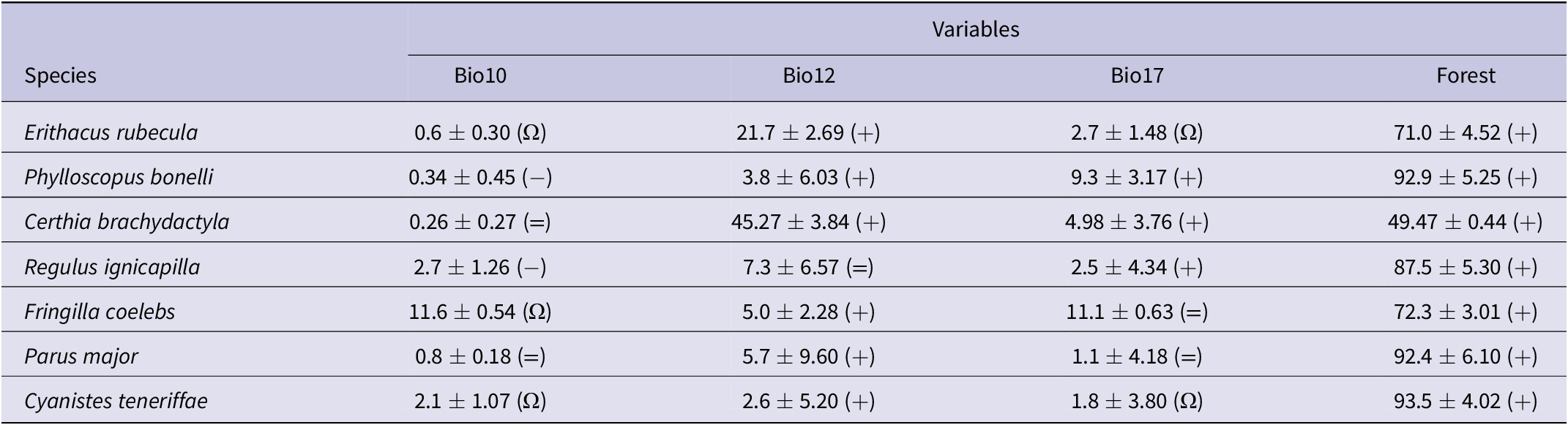
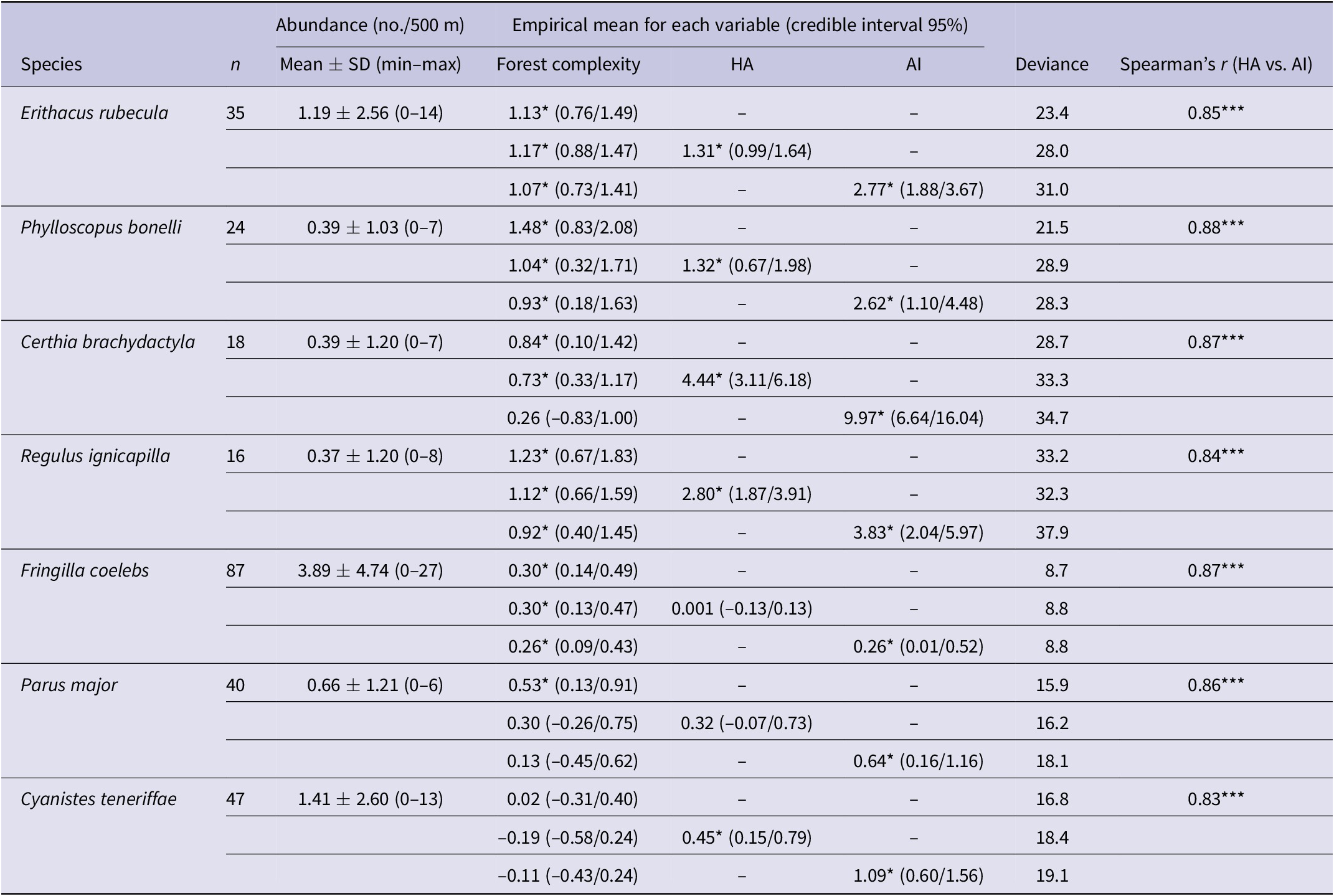
Table 2. Distribution of mean abundance of species based on results from 190 line transects (n = number of line transects with the particular species detected) and the results of multivariate hierarchical Bayesian species zero-inflated distribution models between abundance and local tree cover within the 500-m sampling plot and the potential combinations of habitat amount (HA) and aggregation index (AI) of suitable habitat within a radius of 5 km around the sampling point. Asterisks indicate that the 95% confidence interval around the parameter mean did not include zero (i.e. a significant effect).
Landscape effects on bird abundance
The two landscape metrics (AI and HA) were positively correlated in all species suggesting high aggregation of habitat patches in landscapes with a high percentage of suitable forest (Table 2). Abundance of all birds except for the African Blue Tit showed a significant positive relationship with FC at the study sites (Table 2), but once this effect was accounted for, all species had a significant positive relationship with AI and five out of the seven species were significantly positively correlated with HA (Table 2).
Prospects for change
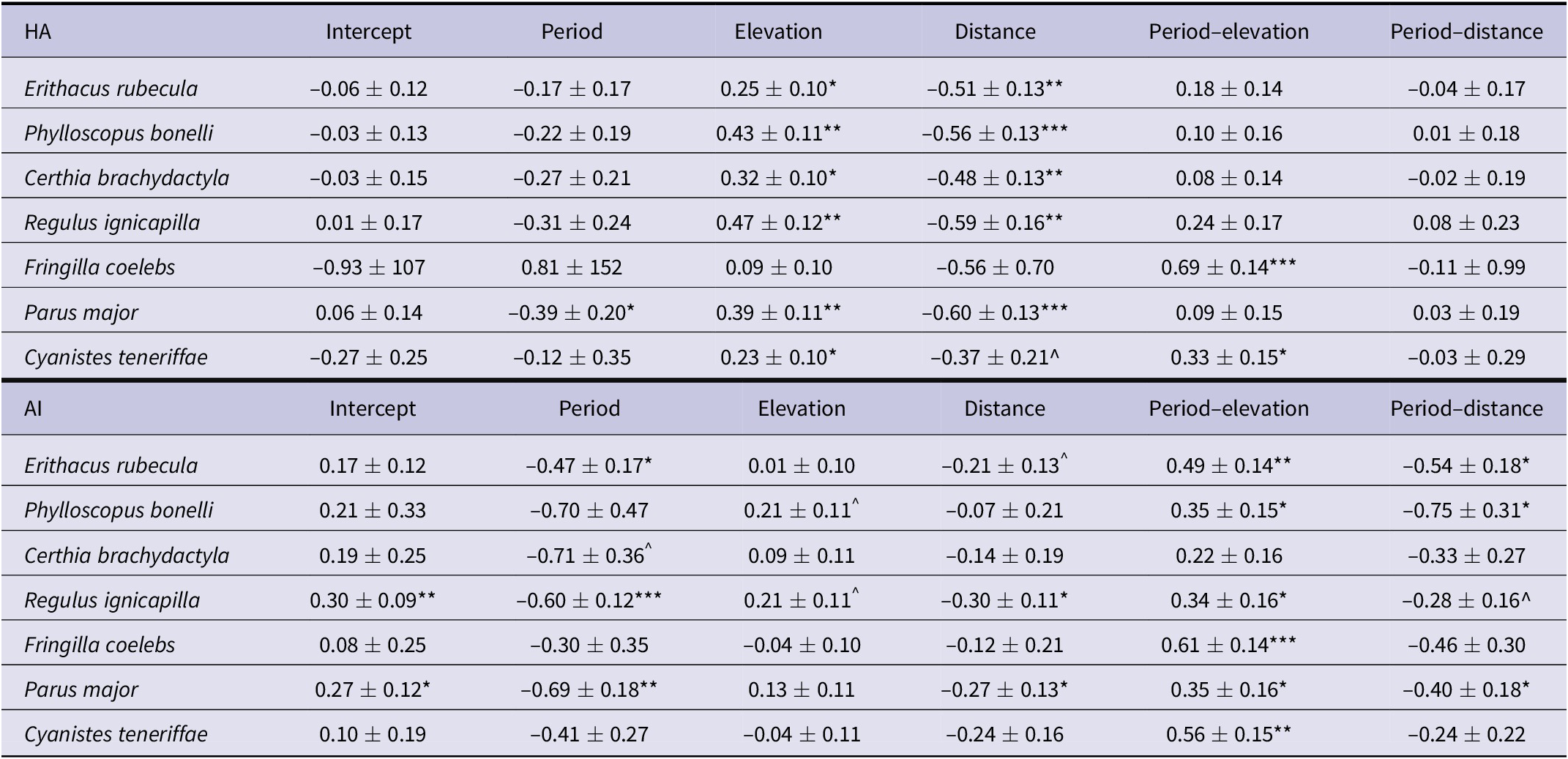
The scores of both landscape metrics (HA and AI) for currently existing distributions decreased southwards in most species and showed fewer discernible increases along elevation (Figure 2). Climate-change projections suggested that HA and AI will show different trends along elevation and distance to the north (see period–elevation and period–distance interactions in Table 3). According to climate projections, HA showed a parallel, non-significant decrease southwards while AI experienced a significant decline in half of the investigated species (Table 3, Figure 2). In the case of elevation, projections suggested that both landscape metrics will experience similar increases in highlands, with significant elevation–period interactions in two species in HA and six species in AI (Table 3). In all species, these projections predicted the depletion of both parameters in lowlands, while they were predicted to maintain or increase their values in highlands (Figure 2).

Figure 2. Relationship between habitat amount (HA) and the aggregation index (AI) with elevation and the distance to the Strait of Gibraltar. Results for two scenarios for the time period are also shown, with blue for current and pink for future time periods.
Table 3. Geographical configuration of suitable habitats. Results are for the coefficients (b ± SE) of the best Generalised Least Squares (GLS) mixed models selected according to Akaike’s information criterion corrected for small sample sizes (AICc), in which the habitat amount (HA) and aggregation index (AI) have been regressed against elevation, distance to the Strait of Gibraltar, and period (current and future conditions). The data have been recorded in 500 random selected circles distributed within the range of species (see Methods). The interactions of period, elevation, and distance have also been calculated to detect potential changes. Significance ^P <0.10, *P <0.05; **P <0.01; ***P <0.001.
Discussion
Habitat and climate change are the two main drivers of the worldwide loss of biodiversity (Sala et al. Reference Sala, Chapin, Armesto, Berlow, Bloomfield, Dirzo and Huber-Sanwald2009). However, even though the damaging effects on biodiversity produced by landscape shifts can be exacerbated in some scenarios due to climate change, both processes have been primarily addressed independently (Travis Reference Travis2003, Opdam and Wascher Reference Opdam and Wascher2004, Mantyka-Pringle et al. Reference Mantyka-Pringle, Martin and Rhodes2012, Sirami et al. Reference Sirami, Caplat, Popy, Clamens, Arlettaz, Jiguet and Brotons2017, Guo et al. Reference Guo, Lenoir and Bonebrake2018, Pettorelli et al. Reference Pettorelli, Graham, Seddon, da Cunha Bustamante, Lowton, Sutherland and Koldewey2021). This appears to be the case for forest organisms at the south-western edge of the Palaearctic, where woodlands resulting from post-glacial climate changes (Hewitt Reference Hewitt1999) and deforestation (Cheddadi et al. Reference Cheddadi, Nourelbait, Bouaissa, Tabel, Rhoujjati, López-Sáez and Alba-Sánchez2015) are now coping with the effects of ongoing climate warming (Carnicer et al. Reference Carnicer, Coll, Ninyerola, Pons, Sanchez and Peñuelas2011, Ruiz-Labourdette et al. Reference Ruiz-Labourdette, Nogués-Bravo, Ollero, Schmitz and Pineda2012). In this context, our results provide some evidence of the synergetic interactions of these two drivers that could exacerbate the difficulties of forest birds to remain in the southern edge of their range.
Effects of landscape structure on bird abundance
We found a positive relationship between bird abundance and HA and AI after accounting for the effect of the fine-grain habitat structure of the sampling sites (FC; Table 2). This relationship is usually explained by the fact that large patches of suitable habitat harbour more individuals than small ones, and because the high connectivity of patches improves the recovery of populations after local extinctions (Hanski Reference Hanski2015). We acknowledge that there is a debate on the relative contribution of these landscape metrics since it has been suggested that in fragmented landscapes HA is the actual driver of species distribution (e.g. Fahrig Reference Fahrig2013, Reference Fahrig2015, Saura Reference Saura2021, Basile et al. Reference Basile, Storch and Mikusiński2021). However, our study has not been designed to disentangle this hypothesis, and we merely show the strong collinearity of both parameters and their effect on bird abundance (Table 2). Thus, as these relationships between HA and connectivity may differ among landscapes (e.g. Wang et al. Reference Wang, Blanchet and Koper2014), our results showed the idiosyncratic landscape patterns of a region where woodlands preferentially occur in northern and mountainous areas and show an increasingly fragmented pattern moving outwards from those areas (Figures 1B and 2). These patterns of landscape depletion emphasise the view provided by the observed decrease southwards of habitat suitability of most forest birds (Tellería et al. Reference Tellería, Hernández-Lambraño and Carbonell2021).
Prospects for change
Climate-change projections suggest that the two landscape metrics (HA and AI) that affect forest bird abundance will experience different trends along elevation and distance to source areas in the north (Figure 2). The loss of HA and connectivity in southern areas forecasts a northward retreat of the range edge in several species, which is a usual prediction on the effect of climate warming in temperate regions (Lenoir and Svenning Reference Lenoir and Svenning2015). In this context, elevation will play a different role because, despite the decrease in HA and connectivity in lowlands, projections show that some species will maintain or even increase these landscape metrics in elevated areas (Figure 2). Habitat shifts upwards in elevation related to mountain ranges have been detected in several species within the south-western Palearctic (Wilson et al. Reference Wilson, Gutiérrez, Gutiérrez, Martínez, Agudo and Monserrat2005). However, beyond the usual withdrawal and reduction of HA in mountain tops (Sekercioglu et al. Reference Sekercioglu, Schneider, Fay and Loarie2008), our results suggest that the hypsographic configuration of north-western Africa (with large expanses above 1500 m) (Figure 1B) will allow areas to expand suitable habitats (Figures 1C and 2). A similar projection has been reported for wintering ranges of some passerines in the south-western Palaearctic, which will expand current ranges upwards as winter temperatures increase (Tellería et al. Reference Tellería, Fernández-López and Fandos2016). Thus, it suggests that shifts of suitable habitat for birds along the western mountain slopes could improve the resilience of bird populations to climate change, a process that explains the role of these mountains as refuge areas during the major climatic fluctuations of the past (Molina-Venegas et al. Reference Molina-Venegas, Aparicio, Lavergne and Arroyo2017).
Conclusions
Our study highlights the importance of landscape management in the conservation of rear-edge populations of forest passerines under a scenario of global change. We acknowledge, however, that the actual consequences of the projected environmental changes are contingent and difficult to predict as they rely on synergetic interactions between human decisions affecting woodland structure, the shortcomings of climate predictions, and the idiosyncratic reaction of species to changes at range edges (Angert et al. Reference Angert, Bontrager and Ågren2020, MacLean and Beissinger Reference MacLean and Beissinger2017, Northrup et al. Reference Northrup, Rivers, Yang and Betts2019). Despite this, our results suggest some basic guidelines aimed to protect forest birds and other forest organisms (Larsen et al. Reference Larsen, Bladt, Balmford and Rahbek2012) at the southern edge of their range. First, in a region strongly affected by human land use, the prevention of forest loss and fragmentation (with the concomitant decrease of habitat amount and connectivity) seems the most obvious approach to protect forest organisms. Second, the uneven geographical patterning of landscape structure advises a preventive/proactive management of southern and lowland woodland landscapes to increase cover and patch connectivity. As in other countries of the south-western Palaearctic, this recovery of woodlands could be assisted in the future by the human abandonment of less productive, marginal areas (Pereira and Navarro Reference Pereira and Navarro2015). Finally, the large mountain ranges involved in these processes can increase forest cover and connectivity in the most elevated areas. This means that any approach to improve tree expansion in highlands could improve the regional resilience of forest organisms to the pervasive effects of climate warming in this peripheral area of the Palaearctic.
Acknowledgements
We thank Roberto Carbonell, who assisted us in several aspects of this study, and three reviewers who considerably improved an early version of this article. This article is a contribution to the project CGL2017- 85637-P (Life at the border: population differentiation of forest birds south of the Palearctic) granted by the Spanish Ministry of Science and Innovation. RHEL has received two grants from Consejería de Educación de la Junta de Castilla y León and Fondo Social Europeo (EDU/556/2019).
Supplementary material
The supplementary material for this article can be found at http://doi.org/10.1017/S0959270923000072.


 Open access