


1 Introduction
Copulas are dependence modelling tools of fundamental importance in actuarial and financial risk management (Frees and Valdez Reference Frees and Valdez1998; Denuit et al. Reference Denuit, Dhaene, Goovaerts and Kaas2006; McNeil et al. Reference McNeil, Frey and Embrechts2015) and fields beyond (e.g. Genest and Favre Reference Genest and Favre2007). An extensive literature has emerged on specifically actuarial applications of copula modelling, in credibility (Frees and Wang Reference Frees and Wang2005), stochastic reserving (Shi and Frees Reference Shi and Frees2011; Shi Reference Shi2014; Abdallah et al. Reference Abdallah, Boucher and Cossette2015), and claims modelling (Czado et al. Reference Czado, Kastenmeier, Brechmann and Min2012; Shi and Valdez Reference Shi and Valdez2014; Hu et al. Reference Hu, Murphy and O’Hagan2021; Tzougas and Pignatelli di Cerchiara Reference Tzougas and Pignatelli di Cerchiara2021). At the same time, the problem of choosing a copula model based on datasets that are of limited size is a non-trivial task, as evidenced in various strands of the literature, indicatively including: seminal work on copula goodness-of-fit (Genest et al. Reference Genest, Rémillard and Beaudoin2009); the study of practical problems arising in insurance risk management (Shaw et al. Reference Shaw, Smith and Spivak2010); the impact of copula choice on portfolio risk (McNeil et al. Reference McNeil, Frey and Embrechts2015, Section 11.1.5); and the consideration of dependence uncertainty in a regulatory framework (Embrechts et al. Reference Embrechts, Puccetti, Rüschendorf, Wang and Beleraj2014). For a historical perspective on the application of copulas to insurance risk modelling, see the interview of Edward (Jed) Frees, by Genest and Scherer (Reference Genest and Scherer2020).
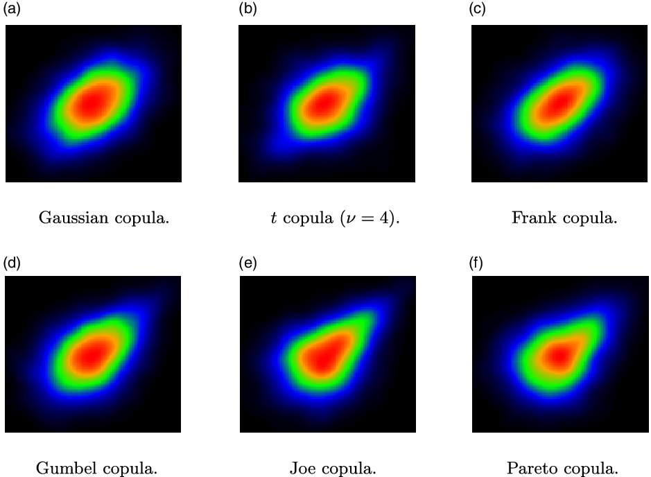
Figure 1. Examples of heatmap images of smoothed bivariate densities for different copula models ( $n=2000, \tau=0.3$
).
$n=2000, \tau=0.3$
).
The different properties of alternative copula models are often visualised by joint density contour plots or heatmaps. For example, in Figure 1, we show heatmap images of smoothed bivariate densities for six well-known copula models, with standard Normal margins. It is obvious that different copula models have heatmaps with different patterns, reflecting for example different degrees of skewness. This observation motivates our research question: Do images of smoothed joint densities convey useful information that can improve the accuracy of copula model selection procedures?
Our paper seeks to address this question, in the context of small data sizes and bivariate copula models. Small data sizes, for example less than 250, make the copula model selection problem hard, hence an improvement offered by image data would be welcome. (Conversely, given the asymptotic consistency of statistical procedures, there is less scope for improvement when data sizes are large.) Furthermore, for small data sizes, it is natural to focus on the simplest models, given the likely lack of statistical power to detect more complex model features. In the case where datasets are richer, the problem the modeller faces is not so much one of selecting between different models, but more one of designing a model that is flexible enough to reflect idiosyncratic features of the data, see for example Hofert et al. (Reference Hofert, Prasad and Zhu2021).
Here, we treat bivariate copula density heatmaps as RGB images and exploit the spatial patterns present in the images to aid bivariate copula selection. The copula selection task is treated as an image recognition or classification task: we classify a given copula sample to an element of a model set, based on its density heatmap image.
One vital challenge in image recognition is to obtain good representations of the images that can summarize well their distinct spatial patterns and thus make the recognition task easier; this is known as representation learning. Deep neural models have been demonstrated to be effective for representation learning, especially in the machine vision community (Bengio et al. Reference Bengio, Courville and Vincent2013). We utilize a deep convolutional neural network, the AlexNet pre-trained by the ImageNet dataset (Krizhevsky et al. Reference Krizhevsky, Sutskever and Hinton2012), to extract image features with strong representation abilities. This is an example of transfer learning, that is, the use of knowledge from addressing a particular problem, to a new task (Pan and Yang Reference Pan and Yang2009; Zhuang et al. Reference Zhuang, Qi, Duan, Xi, Zhu, Zhu, Xiong and He2020).
Instead of using the extracted image features to train a classifier directly, we propose three additional amendments on them. First, the AlexNet image features are high dimensional. To avoid potential problems induced by high dimensionality, principal component analysis (PCA) (Wold et al. Reference Wold, Esbensen and Geladi1987) is applied to reduce the dimensions of the extracted image features. Second, to further enhance the representation ability of the features, summary statistics are concatenated with image features to provide a more complete description of copula samples. Lastly, we aim to make these features more discriminative via linear discriminant analysis (LDA), which projects the concatenated features to a low-dimensional subspace where the observations from the same classes are grouped close together, while those from different classes are pushed apart (Yang and Jin Reference Yang and Jin2006). Hence, the recognition task becomes easier on this discriminative subspace. The features extracted by LDA are used as the final representations of the copula samples to train the classifier. Support vector machine (SVM) is chosen as the classifier for the image recognition task, because it is proven to be effective on various real-world applications (Tzotsos and Argialas Reference Tzotsos and Argialas2008; Islam et al. Reference Islam, Dinh, Wahid and Bhowmik2017; Sheykhmousa et al. Reference Sheykhmousa, Mahdianpari, Ghanbari, Mohammadimanesh, Ghamisi and Homayouni2020).
We test the performance of the proposed image recognition approach to copula selection via simulation studies. We consider the six copula models of Figure 1 and evaluate the classification accuracy of our approach in different scenarios, comparing to the statistical benchmark given by AIC. First, we consider model selection when all training and testing instances arise for copula samples with the same sample size and underlying rank correlation. While this is not a realistic setting, it allows us to explore the performance of image recognition for different problem parameters. We observe that image recognition consistently outperforms AIC, except when the underlying rank correlation is very high. The biggest improvement occurs in those scenarios of low sample size and correlation, where the copula selection problem is the hardest.
Subsequently, we consider a more realistic scenario, where a copula model needs to be selected for data with differing sample sizes and correlations, generated under any rotation of the six bivariate baseline copula models. In this scenario, the heatmap images from the same copula model can present very different patterns, leading to substantial within-class variations. For that reason, we propose to add a first data rotation step, based on sample statistics, with the aim of converting the data to be positively correlated and skewed. Then, in a second step, we apply the image recognition approach to images generated from the rotated data.
We find that this two-step image recognition approach dominates AIC for the copula model selection task, again except in the situation of high correlations. This motivates our final proposal to combine the two-step image recognition approach with AIC. In this combined approach, AIC values (calculated on the rotated data) are concatenated with the image features and statistical features before applying LDA. Experiments show that the combined approach improves on both AIC and image recognition-based model selection.
Finally, we apply the copula selection framework developed in the paper to modelling joint weekly losses of the MSCI World Index and the ICMR (Re)Insurance Specialty Index. The dependence between those two indices is important as it reflects inter-industry diversification and thus (re)insurers’ capital availability. We find that both the strength of correlation and the copula family selected vary over time, with the t copula being the most frequent choice.
The paper is organised as follows. In Section 2, we give preliminaries on copula modelling. Section 3 introduces the image recognition approach, with fixed correlation and sample sizes. In Section 4, we discuss the two-step approach to copula model selection for more general datasets. Experimental results are summarised within each section. The real-data application is presented in Section 5. Section 6 presents our concluding remarks.
2 Copulas
2.1 Copula models and their properties
Consider continuous random variables X,Y with marginal distributions $F,\;G$
and joint distribution H, on a probability space
$F,\;G$
and joint distribution H, on a probability space $(\Omega,\mathcal F,\mathbb{P})$
. The copula of (X,Y) is a distribution on
$(\Omega,\mathcal F,\mathbb{P})$
. The copula of (X,Y) is a distribution on $[0,1]^2$
with uniform marginals, such that
$[0,1]^2$
with uniform marginals, such that
 \begin{align} H(x,y)=C(F(x),G(y)).\end{align}
Denote $U=F(X),\;V=G(Y)$
and also
$U=F(X),\;V=G(Y)$
and also $\bar U=1-U,\;\bar V=1-V$
. Then it follows from (2.1) that C is the joint distribution of (U,V), that is,
$\bar U=1-U,\;\bar V=1-V$
. Then it follows from (2.1) that C is the joint distribution of (U,V), that is,
 \begin{align} C(u,v)=\mathbb{P}(U\leqslant u, V\leqslant v),\quad (u,v) \in [0,1]^2.\end{align}
Analogously, the joint distribution of $(\bar U,\bar V)$
is called the survival copula of (X,Y) and denoted by
$(\bar U,\bar V)$
is called the survival copula of (X,Y) and denoted by $\bar C$
.
$\bar C$
.
Definition (2.1) implies a separation of a random vector’s marginal behaviour from its dependence structure, which has enabled copulas to be widely employed as multivariate modelling tools. For detailed treatments of copulas, including applications in insurance and financial risk management, see Nelsen (Reference Nelsen2007), Denuit et al. (Reference Denuit, Dhaene, Goovaerts and Kaas2006), McNeil et al. (Reference McNeil, Frey and Embrechts2015). We note that the copulas of discontinuous random vectors are not uniquely defined – in such a case the variables $U,\;V$
as constructed above are not uniform. However, we can always uniquely determine a copula for X,Y via (2.2), with uniform variables U,V constructed via the generalised distributional transform of Rüschendorf and de Valk (Reference Rüschendorf and de Valk1993).Footnote 1
$U,\;V$
as constructed above are not uniform. However, we can always uniquely determine a copula for X,Y via (2.2), with uniform variables U,V constructed via the generalised distributional transform of Rüschendorf and de Valk (Reference Rüschendorf and de Valk1993).Footnote 1
In risk management, the specific properties of different copula families are important. Assume that X and Y represent losses, such that high (joint) outcomes are associated with adverse events. Then, beyond considering (rank) correlation measures, it is important to model the extent to which X and Y will jointly achieve high values. A typical way in which the literature considers the propensity of joint extremes is via the coefficients of upper and lower tail dependence (e.g. McNeil et al. Reference McNeil, Frey and Embrechts2015, Section 7.2.4):
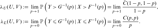 \begin{align*} \lambda_U(U,V)&\;:\!=\; \lim_{p\to 1}\mathbb{P}\left(Y> G^{-1}(p)\;|\;X> F^{-1}(p)\right)=\lim_{p\to 1}\frac{\bar C(1-p,1-p)}{1-p},\\ \lambda_L(U,V)&\;:\!=\; \lim_{p\to 0}\mathbb{P}\left(Y\leqslant G^{-1}(p)\;|\;X\leqslant F^{-1}(p)\right)=\lim_{p\to 0}\frac{ C(p,p)}{p}.\end{align*}
Models for which $\lambda_U$
or
$\lambda_U$
or $\lambda_L$
are non-zero are, respectively, called upper or lower tail dependent.
$\lambda_L$
are non-zero are, respectively, called upper or lower tail dependent.
While tail dependence is an asymptotic property, a distinct issue is the skewness or asymmetry of a copula. A copula is radially symmetric if $C(1-u,1-v)=C(u,v)$
. Various measures of bivariate skewness have been proposed by Rosco and Joe (Reference Rosco and Joe2013). Here we focus on the moment-based measure
$C(1-u,1-v)=C(u,v)$
. Various measures of bivariate skewness have been proposed by Rosco and Joe (Reference Rosco and Joe2013). Here we focus on the moment-based measure $\zeta$
, defined for
$\zeta$
, defined for $k \in (1,\infty)$
as:
$k \in (1,\infty)$
as:
 \begin{align*} \zeta(U,V;k) =\mathbb{E} \left[|U+V-1|^k \textrm{sign}(U+V-1) \right].\end{align*}
Implications of the choice of the parameter k are briefly explored in Rosco and Joe (Reference Rosco and Joe2013).
A further property of bivariate copulas relates to the extent that observations are concentrated in the four corners of the unit box, even when correlation is low, leading to spider-like pattern. This property, which distinguishes, for example, a t from a Gaussian copula model, is termed arachnitude in Shaw et al. (Reference Shaw, Smith and Spivak2010), see also Androschuck et al. (Reference Androschuck, Gibbs, Katrakis, Lau, Oram, Raddall, Semchyshyn, Stevenson and Waters2017), Genest et al. (Reference Genest, Nešlehová, Rémillard and Murphy2019). We measure arachnitude in the way proposed by Shaw et al. (Reference Shaw, Smith and Spivak2010), that is, as
 \begin{align*} \xi(U,V)\;:\!=\;\rho\left((U-0.5)^2,(V-0.5)^2\right),\end{align*}
where $\rho$
is the Pearson (product-moment) correlation.
$\rho$
is the Pearson (product-moment) correlation.
In this paper, we consider six bivariate copula models:
-
1. The Gaussian copula is probably the most widely used copula model. It is radially symmetric and tail independent.
-
2. The t copula is radially symmetric but both upper- and lower-tail dependent. It admits a degree of freedom parameter $\nu$
;
$\lambda_L, \lambda_U$
decrease in
$\nu$
, while for
$\nu \to \infty$
, the t copula reduces to a Gaussian.
$\nu$
;
$\lambda_L, \lambda_U$
decrease in
$\nu$
, while for
$\nu \to \infty$
, the t copula reduces to a Gaussian. -
3. The Frank copula is radially symmetric and tail independent.
-
4. The Gumbel copula, commonly used in risk management, is positively skewed and upper tail dependent.
-
5. The Joe copula is positively skewed and upper tail dependent.
-
6. The Pareto copula (or Clayton survival copula), is positively skewed and upper tail dependent.


We do not provide technical detail on these models, as they are all well known and exhaustively discussed in the literature (Denuit et al. Reference Denuit, Dhaene, Goovaerts and Kaas2006; Nelsen Reference Nelsen2007; McNeil et al. Reference McNeil, Frey and Embrechts2015). The Gaussian and t models are, respectively, the copulas of bivariate Normal and t distributions; the remaining four models belong to the family of Archimedean copulas. All models, except the t copula, have a single parameter, which can be calibrated to (e.g. Kendall’s) rank correlation or estimated by MLE. The t model has the degrees of freedom $\nu$
as an additional parameter.
$\nu$
as an additional parameter.
The properties of different copula families are illustrated in Figure 1, which shows heatmaps of smoothed bivariate densities, each derived from samples of size $n=2000$
, with underlying Kendall rank correlation
$n=2000$
, with underlying Kendall rank correlation $\tau=0.3$
. While copulas are defined as distributions with uniform marginals, here and in the sequel, before producing such plots, we transform the marginals to standard normals, as we find that this transformation enables a better visual inspection of the dependence pattern. The distinct patterns of the different models are visible. At the same time, there is substantial similarity between some of the resulting heatmaps (e.g. Gaussian and t; Joe and Pareto), which indicates that selecting the correct model from data is not a trivial task. This is of course even more challenging for smaller datasets. We show heatmaps from the Gaussian and t families in Figure 2, comparing plots generated from bivariate samples of sizes
$\tau=0.3$
. While copulas are defined as distributions with uniform marginals, here and in the sequel, before producing such plots, we transform the marginals to standard normals, as we find that this transformation enables a better visual inspection of the dependence pattern. The distinct patterns of the different models are visible. At the same time, there is substantial similarity between some of the resulting heatmaps (e.g. Gaussian and t; Joe and Pareto), which indicates that selecting the correct model from data is not a trivial task. This is of course even more challenging for smaller datasets. We show heatmaps from the Gaussian and t families in Figure 2, comparing plots generated from bivariate samples of sizes $n=100$
and 2000. It is apparent that with the smaller sample size the observed patterns become substantially noisier.
$n=100$
and 2000. It is apparent that with the smaller sample size the observed patterns become substantially noisier.
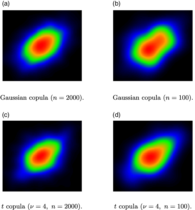
Figure 2. Comparison of heatmap images of smoothed bivariate densities for sample sizes $n=100, 2000$
(
$n=100, 2000$
( $\tau=0.3$
).
$\tau=0.3$
).
2.2 Estimation and model selection
Consider a sample from (X,Y), $(x_1,y_1), \dots, (x_n,y_n)$
. Realisations of the random vector (U,V) are not directly observable.Footnote 2 As a result, it is common to construct copula pseudo-observations (e.g. Genest et al. Reference Genest, Rémillard and Beaudoin2009). Let
$(x_1,y_1), \dots, (x_n,y_n)$
. Realisations of the random vector (U,V) are not directly observable.Footnote 2 As a result, it is common to construct copula pseudo-observations (e.g. Genest et al. Reference Genest, Rémillard and Beaudoin2009). Let $r_i(\mathbf z)$
be the rank of observation
$r_i(\mathbf z)$
be the rank of observation $z_i$
in a univariate sample
$z_i$
in a univariate sample $\mathbf z=(z_1,\dots,z_n)$
. Then, the pseudo-observations are given by
$\mathbf z=(z_1,\dots,z_n)$
. Then, the pseudo-observations are given by
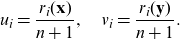 \begin{align*} u_i= \frac{r_i(\mathbf x)}{n+1}, \quad v_i= \frac{r_i(\mathbf y)}{n+1}.\end{align*}
From the pseudo-observations $(u_i,v_i),\;i=1,\dots,n$
, we can readily estimate skewness and arachnitude, denoting the corresponding estimates by
$(u_i,v_i),\;i=1,\dots,n$
, we can readily estimate skewness and arachnitude, denoting the corresponding estimates by $\hat \zeta,\; \hat \xi$
. Furthermore, we denote the sample version of Kendall’s rank correlation as
$\hat \zeta,\; \hat \xi$
. Furthermore, we denote the sample version of Kendall’s rank correlation as $\hat \tau$
.
$\hat \tau$
.
From the observations $(u_i,v_i),\;i=1,\dots,n$
, we can readily estimate skewness and arachnitude, denoting the corresponding estimates by
$(u_i,v_i),\;i=1,\dots,n$
, we can readily estimate skewness and arachnitude, denoting the corresponding estimates by $\hat \zeta,\; \hat \xi$
. Furthermore, we denote the sample version of Kendall’s rank correlation as
$\hat \zeta,\; \hat \xi$
. Furthermore, we denote the sample version of Kendall’s rank correlation as $\hat \tau$
.
$\hat \tau$
.
For a parametric family of copulas $C^{(m)}(\cdot;\theta),\;\theta \in \Theta_m$
, the parameters
$C^{(m)}(\cdot;\theta),\;\theta \in \Theta_m$
, the parameters $\theta$
can be estimated by maximum likelihood estimation, treating the pseudo-observations as if they are a random sample from
$\theta$
can be estimated by maximum likelihood estimation, treating the pseudo-observations as if they are a random sample from $C^{(m)}(\cdot;\theta)$
. If we are considering a family of copula models
$C^{(m)}(\cdot;\theta)$
. If we are considering a family of copula models $\{C^{(m)},\;m \in \mathcal M\}$
, likelihood methods also offer model selection criteria. Let
$\{C^{(m)},\;m \in \mathcal M\}$
, likelihood methods also offer model selection criteria. Let $c^{(m)}$
be the bivariate density corresponding to copula
$c^{(m)}$
be the bivariate density corresponding to copula $C^{(m)}$
and
$C^{(m)}$
and $\hat \theta^{(m)}$
the (
$\hat \theta^{(m)}$
the ( $k_m$
-dimensional) estimate of the corresponding model parameter. The Akaike and Bayes Information criteria are given by
$k_m$
-dimensional) estimate of the corresponding model parameter. The Akaike and Bayes Information criteria are given by
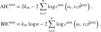 \begin{align*} \textrm{AIC}^{(m)}&=2k_m-2\sum_{i=1}^n\log c^{(m)}\left(u_i,v_i;\hat \theta ^{(m)}\right),\\ \textrm{BIC}^{(m)}&=k_m\log n -2\sum_{i=1}^n\log c^{(m)}\left(u_i,v_i;\hat \theta ^{(m)}\right).\end{align*}
The selected model is then the one with the lowest $\textrm{AIC}^{(m)}$
or
$\textrm{AIC}^{(m)}$
or $\textrm{BIC}^{(m)}$
. A cross-validated log-likelihood criterion is formulated by (Grønneberg and Hjort 2014, Equation (42)); see Jordanger and Tjøstheim (2014) for a simulation study. Other model selection criteria can be constructed using goodness-of-fit statistics; for example Kularatne et al. (Reference Kularatne, Li and Pitt2021) employ the Cramer-von Mises statistic, the use of which (including variations) in copula goodness-of-fit testing has been thoroughly explored by Genest et al. (Reference Genest, Rémillard and Beaudoin2009). Bayesian copula selection is discussed in Huard et al. (Reference Huard, Evin and Favre2006).
$\textrm{BIC}^{(m)}$
. A cross-validated log-likelihood criterion is formulated by (Grønneberg and Hjort 2014, Equation (42)); see Jordanger and Tjøstheim (2014) for a simulation study. Other model selection criteria can be constructed using goodness-of-fit statistics; for example Kularatne et al. (Reference Kularatne, Li and Pitt2021) employ the Cramer-von Mises statistic, the use of which (including variations) in copula goodness-of-fit testing has been thoroughly explored by Genest et al. (Reference Genest, Rémillard and Beaudoin2009). Bayesian copula selection is discussed in Huard et al. (Reference Huard, Evin and Favre2006).
In this paper, we use as a statistical benchmark for model selection the AIC.Footnote 3
3 An image recognition-based approach to copula model selection
In this section, we introduce a new methodology, which uses image recognition to select a suitable bivariate copula from a sample, by classifying its density heatmap image to one of the six models we consider. The recognition process is designed to incorporate rich information that can well represent the samples and is discriminative to make the classification task easier. The generation of the heatmap images is introduced first, and then the image recognition approach is discussed in detail. Subsequently, experimental results are shown to demonstrate the effectiveness of this approach for copula model selection.
We note that in the present section we apply the classification/copula model selection framework to simulated data with very benign features, with all images in any given dataset derived from samples with the same sample size and underlying correlation. This is of course an unrealistic testing environment, with classes that are more homogeneous than in any practical application. Nonetheless, the setting of this section allows us to evaluate whether image recognition can be effective as a copula selection tool (and under which conditions). The restrictive assumptions of this section are relaxed in the two-step approach of Section 4.
3.1 Generating heatmap images of smoothed bivariate densities
Here we outline how the image datasets are generated, on which classifiers are trained to perform the copula selection task. Each image is a smoothed bivariate density heatmap, generated from a simulated pseudo-sample from (U,V), drawn from a given copula specification $C^{(m)}(\cdot;\theta),\;\theta \in \Theta^{(m)},\;m \in \mathcal M$
.
$C^{(m)}(\cdot;\theta),\;\theta \in \Theta^{(m)},\;m \in \mathcal M$
.
For each image dataset that we generate the following hold:
-
(a) The dataset contains
$R=20,000$
images. -
(b) Each image is derived from a bivariate sample of size n, drawn from one of the 6 copula families we consider in this paper,
$\mathcal M=\mathcal M_s \cup \mathcal M_a$
, where
$\mathcal M_s= \{\textrm{Gaussian, } t\textrm{, Frank}\}$
and
$\mathcal M_a=\{\textrm{Gumbel, Joe, Pareto}\}$
contain radially symmetric and asymmetric (positively skewed) models respectively. Each dataset contains approximately the same number of images from each copula family. -
(c) In each dataset, all images are generated from simulated samples with a fixed sample size
$n \in \{100,150, 200, 250\}$
and (population) Kendall
$\tau \in \{0.1,0.3,0.5,0.7,0.9\}$
. Hence we have
$4\times 5 =20$
datasets, corresponding to different
$(n,\tau)$
combinations, each containing R images. -
(d) All images are generated from bivariate samples that have positive empirical rank correlation and positive empirical skewness. This means that samples that display negative rank correlation are rejected and not used to produce images in the dataset. Furthermore, samples that display negative sample skewness, when the underlying copula model has positive skewness, are also rejected.Footnote 4
-
(e) Images are generated based on pseudo-observations from the copula samples. Furthermore, to generate the heatmap images, we transform pseudo-observations to have a standard normal marginal distribution. This transformation is employed only for image generating purposes and reflects no assumption of normality for the marginal distribution of the underlying data.


The precise process by which images are generated is given in the Supplementary Material (Appendix C, Algorithm 1). All calculations are carried out in R. For random number generation we use package copula (Yan Reference Yan2007; Hofert et al. Reference Hofert, Kojadinovic, Maechler and Yan2020). For AIC calculations, we use the package VineCopula (Schepsmeier et al. Reference Schepsmeier, Stoeber, Brechmann, Graeler, Nagler, Erhardt, Almeida, Min, Czado, Hofmann, Killiches, Joe and Vatter2021).
Joint densities are estimated on a 100 $\times$
100 grid on
$\times$
100 grid on $[-3,3]^2$
using an axis-aligned bivariate normal kernel, by the function kde2d of the package MASS, with bandwidths set to 1.3 times the values given by the heuristic in (Venables and Ripley Reference Venables and Ripley2002, Equation (5.5)). Specifically, for a bivariate sample
$[-3,3]^2$
using an axis-aligned bivariate normal kernel, by the function kde2d of the package MASS, with bandwidths set to 1.3 times the values given by the heuristic in (Venables and Ripley Reference Venables and Ripley2002, Equation (5.5)). Specifically, for a bivariate sample $(x_j,y_j),\;j=1,\dots,n,$
the density estimate at an arbitrary point (x,y) is given by
$(x_j,y_j),\;j=1,\dots,n,$
the density estimate at an arbitrary point (x,y) is given by
 \begin{equation*}f(x,y) =\sum_{j=1}^n\frac{\varphi\big((x-x_j)/h_x \big)\varphi\big((y-y_j)/h_y \big)}{h_xh_y},\end{equation*}
where $\varphi$
is the standard normal density and
$\varphi$
is the standard normal density and $h_x,h_y$
are the bandwidths used. Subsequently, the values of the bivariate density estimate f on the grid are used to generate a heatmap, via the image function. The heatmap consists of a 100
$h_x,h_y$
are the bandwidths used. Subsequently, the values of the bivariate density estimate f on the grid are used to generate a heatmap, via the image function. The heatmap consists of a 100 $\times$
100 grid of coloured rectangles with colours corresponding to the values of the density estimate. The heatmap is then saved as a png image file.
$\times$
100 grid of coloured rectangles with colours corresponding to the values of the density estimate. The heatmap is then saved as a png image file.
3.2 The image recognition approach
Now we present the image recognition approach with the complete workflow shown in Figure 3. Similarly to all classification tasks, the image recognition approach consists of a training phase to extract features and train a classifier, and a test phase to predict a copula model for a test sample. In Figure 3, the training phase is presented by the black flow while the test phase is presented by the red flow.
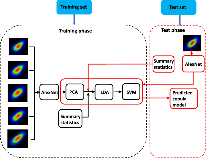
Figure 3. The workflow of the image recognition approach for copula model selection.
3.2.1 The training phase
The training phase contains two parts: (1) the representation learning part to extract features with strong representation and discrimination abilities and (2) the classification part to train an effective classifier.
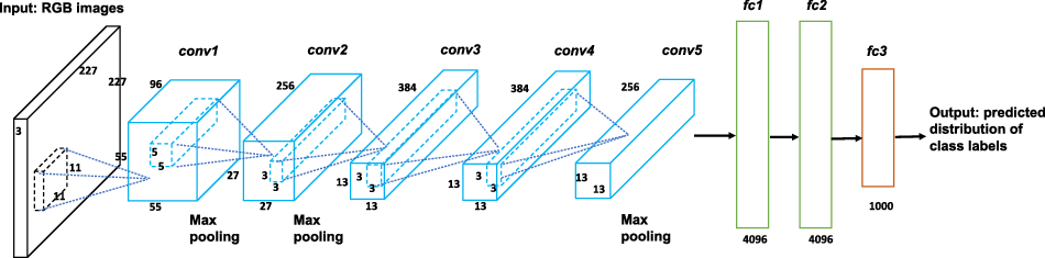
Figure 4. The architecture of the AlexNet.
Representation learning. In the representation learning part, two types of features are extracted from the training copula samples: pure image features and statistical features. The pure image features are extracted from the training heatmap images by the pretrained AlexNet that has been trained on the ImageNet dataset with 1000 classes of high-resolution images (Deng et al. Reference Deng, Dong, Socher, Li, Li and Fei-Fei2009). Given the complex nature of the images in the ImageNet dataset and the competitive classification performance of AlexNet, we believe that this pretrained network can provide good representations of our heatmap images of relatively simple patterns.
AlexNet is a deep convolutional neural network, consisting of layers with three-dimensional volumes of neurons. The architecture of AlexNet is depicted in Figure 4, with an input layer of RGB images, five convolutional layers and three fully connected layers. The input layer is of dimension $227 \times 227 \times 3$
: 227 and 227 are the width and height of the layer, which represent the width and height of the image, while 3 is the depth of the layer, representing the red, green and blue channels of the RGB image. The convolutional layer contains neurons that are only connected to a small local region in the previous layer, each computing a dot product between the filters and the region they are connected to, that is the convolution between the filters and input regions. Let us take the first convolutional layer as an example. The filters of this layer are of dimension
$227 \times 227 \times 3$
: 227 and 227 are the width and height of the layer, which represent the width and height of the image, while 3 is the depth of the layer, representing the red, green and blue channels of the RGB image. The convolutional layer contains neurons that are only connected to a small local region in the previous layer, each computing a dot product between the filters and the region they are connected to, that is the convolution between the filters and input regions. Let us take the first convolutional layer as an example. The filters of this layer are of dimension $11 \times 11 \times 3$
and each of them captures different features from the input image, for example edge or colour. By sliding each filter across the width and height of the input layer and applying the convolution operation, we can obtain a two-dimensional activation map that contains the responses of the filter at every spatial position. Specifically, we reshape the
$11 \times 11 \times 3$
and each of them captures different features from the input image, for example edge or colour. By sliding each filter across the width and height of the input layer and applying the convolution operation, we can obtain a two-dimensional activation map that contains the responses of the filter at every spatial position. Specifically, we reshape the $11 \times 11 \times 3$
volume of the input and filter to two
$11 \times 11 \times 3$
volume of the input and filter to two $11 \times 11 \times 3 = 363$
dimensional column vectors. The dot product of the two vectors is fed to the RELU activation function,
$11 \times 11 \times 3 = 363$
dimensional column vectors. The dot product of the two vectors is fed to the RELU activation function, $\max \{0,x \}$
, to capture the nonlinearity of features. The output from the activation function is called activation and fills one entry in the activation map. This process leads to a volume of
$\max \{0,x \}$
, to capture the nonlinearity of features. The output from the activation function is called activation and fills one entry in the activation map. This process leads to a volume of $55 \times 55 \times 96$
neurons in the first convolutional layer, with 96 filters. The max pooling layers between the convolutional layers can effectively reduce the number of parameters and control overfitting.
$55 \times 55 \times 96$
neurons in the first convolutional layer, with 96 filters. The max pooling layers between the convolutional layers can effectively reduce the number of parameters and control overfitting.
The outputs of the convolutional layers are then fed to fully connected layers to provide the predicted distribution of the class labels, that is the predicted probabilities for each of the 1000 classes considered. Note that we do not use the classification output of AlexNet, as the 1000 classes used are not relevant to our copula selection task; however, the representation ability of the network allows us to use it for feature extraction from our heatmap images. To demonstrate the good representation ability of the pretrained AlexNet, we show the activation maps of a Gaussian copula sample for all 96 filters of the first convolutional layer in Figure 5, with each square presenting the activation map of one filter. The bright pixels reflect high activations, which means that they make substantial contributions to the extracted features. It is obvious that the contour shapes of the Gaussian sample can be well captured by the first convolutional layer.
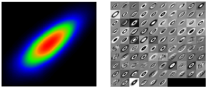
Figure 5. Left: The heatmap image of a Gaussian copula sample. Right: The activations of the first convolutional layer of AlexNet for the sample.
We input the training heatmap images to the pretrained AlexNet, and extract 4096 features from the second fully connected layer, ‘fc2’ in Figure 4, which is the last feature extraction layer before working out predicted probabilities. This layer provides high-level abstract features that can well represent the images. To be precise, each training heatmap image is represented by a 4096-dimensional vector $\mathbf{x}^{M}_i \in \mathbb{R}^{4096 \times 1}$
(
$\mathbf{x}^{M}_i \in \mathbb{R}^{4096 \times 1}$
( $i = 1,2,\ldots, N$
), where N is the number of training copula samples, and the image features of the whole training set is denoted as
$i = 1,2,\ldots, N$
), where N is the number of training copula samples, and the image features of the whole training set is denoted as $\mathbf{X}^{M}=[\mathbf{x}^{M}_1,\mathbf{x}^{M}_2,\ldots,\mathbf{x}^{M}_N]^T \in \mathbb{R}^{N \times 4096}$
. (Note that N here is different to the size of the whole data set R, as the generated images for each dataset will be subsequently split into training and test samples.)
$\mathbf{X}^{M}=[\mathbf{x}^{M}_1,\mathbf{x}^{M}_2,\ldots,\mathbf{x}^{M}_N]^T \in \mathbb{R}^{N \times 4096}$
. (Note that N here is different to the size of the whole data set R, as the generated images for each dataset will be subsequently split into training and test samples.)
The high number of image features can lead to potential problems in classification, for example the curse of dimensionality and high computational cost. Thus, we reduce the number of image features before training a classifier. This dimension reduction step is achieved by principal component analysis (PCA), which is a widely adopted unsupervised dimension reduction method that can provide low-dimensional yet effective representations of the original high-dimensional data (Wold et al. Reference Wold, Esbensen and Geladi1987). PCA projects data from the original feature space to a low-dimensional subspace, spanned by the first few principal components (PCs) that can explain most of the variation in data. This can be achieved by applying the reduced singular value decomposition (SVD) on the column-centred $\mathbf{X}^M$
. Let
$\mathbf{X}^M$
. Let $\mathbf{V}$
denote the matrix whose columns are the PCs sorted by the singular values in a descending order. In this paper, we set
$\mathbf{V}$
denote the matrix whose columns are the PCs sorted by the singular values in a descending order. In this paper, we set $q=150$
to explain 99.9% of the variation in
$q=150$
to explain 99.9% of the variation in $\mathbf{X}^M$
. After PCA, the image features of the training set become
$\mathbf{X}^M$
. After PCA, the image features of the training set become
 \begin{equation}\mathbf{X}^{MP}=(\mathbf{X}^M)^c \mathbf{V}_{150} \in \mathbb{R}^{N \times 150},\end{equation}
where $(\mathbf{X}^M)^c$
is derived by subtracting the column means of
$(\mathbf{X}^M)^c$
is derived by subtracting the column means of $\mathbf{X}^M$
,
$\mathbf{X}^M$
, $\mathbf{V}_{150} \in \mathbb{R}^{4096 \times 150}$
is
$\mathbf{V}_{150} \in \mathbb{R}^{4096 \times 150}$
is $\mathbf{V}$
with the first 150 columns. Thus, the image features now lie in a 150-dimensional PC subspace.
$\mathbf{V}$
with the first 150 columns. Thus, the image features now lie in a 150-dimensional PC subspace.
Besides the pure image features extracted from AlexNet, we propose to utilise some additional statistical features to enrich the description of the training copula samples. Three summary statistics, Kendall’s rank correlation, skewness and arachnitude are chosen as the statistical features. The statistical features of each sample are denoted as $\mathbf{x}^{S}_i=(\hat \tau_i,\hat \zeta_i,\hat\xi_i) \in \mathbb{R}^{3 \times 1}, i = 1,2,\ldots, N$
.
$\mathbf{x}^{S}_i=(\hat \tau_i,\hat \zeta_i,\hat\xi_i) \in \mathbb{R}^{3 \times 1}, i = 1,2,\ldots, N$
.
The low-dimensional image features and three statistical features are then concatenated to provide a representation for the ith copula sample, $\mathbf{x}_i=[(\mathbf{x}^{MP}_i)^T,(\mathbf{x}^{S}_i)^T]^T \in \mathbb{R}^{153 \times 1}$
, where
$\mathbf{x}_i=[(\mathbf{x}^{MP}_i)^T,(\mathbf{x}^{S}_i)^T]^T \in \mathbb{R}^{153 \times 1}$
, where $\mathbf{x}^{MP}_i \in \mathbb{R}^{150 \times 1}$
is the ith observation in
$\mathbf{x}^{MP}_i \in \mathbb{R}^{150 \times 1}$
is the ith observation in $\mathbf{X}^{MP}$
. The feature matrix to represent all training copula samples is denoted as
$\mathbf{X}^{MP}$
. The feature matrix to represent all training copula samples is denoted as $\mathbf{X}=[\mathbf{x}_1,\mathbf{x}_2,\ldots,\mathbf{x}_N]^T \in \mathbb{R}^{N \times 153}$
. Before simply feeding this feature matrix to a classifier, we extract more compact and discriminative information to reflect the differences between classes better and make the classification process easier. For that purpose, we apply LDA on
$\mathbf{X}=[\mathbf{x}_1,\mathbf{x}_2,\ldots,\mathbf{x}_N]^T \in \mathbb{R}^{N \times 153}$
. Before simply feeding this feature matrix to a classifier, we extract more compact and discriminative information to reflect the differences between classes better and make the classification process easier. For that purpose, we apply LDA on $\mathbf{X}$
. LDA is a well known supervised dimension reduction method that projects data to a subspace such that between-class variation is maximised while within-class variation is minimised (Yang and Jin Reference Yang and Jin2006). The classification task is easier on this subspace because the instances from the same class are pulled close together while those from different classes are pushed further away. By projecting
$\mathbf{X}$
. LDA is a well known supervised dimension reduction method that projects data to a subspace such that between-class variation is maximised while within-class variation is minimised (Yang and Jin Reference Yang and Jin2006). The classification task is easier on this subspace because the instances from the same class are pulled close together while those from different classes are pushed further away. By projecting $\mathbf{X}$
on the linear discriminant subspace, we have
$\mathbf{X}$
on the linear discriminant subspace, we have
 \begin{equation}\mathbf{X}^P = \mathbf{X} \mathbf{W} \in \mathbb{R}^{N \times (K-1)},\end{equation}
where $\mathbf{W} \in \mathbb{R}^{153 \times (K-1)}$
contains the bases of the linear discriminant subspace and K is the number of classes. LDA can provide at most a
$\mathbf{W} \in \mathbb{R}^{153 \times (K-1)}$
contains the bases of the linear discriminant subspace and K is the number of classes. LDA can provide at most a $(K-1)$
-dimensional subspace. In this paper, six copula models are considered, thus the LDA subspace is at most five-dimensional. Here, we take all five discriminative dimensions provided by LDA.
$(K-1)$
-dimensional subspace. In this paper, six copula models are considered, thus the LDA subspace is at most five-dimensional. Here, we take all five discriminative dimensions provided by LDA.
Classification. Support vector machine (SVM) is chosen as the classifier for its efficiency in many real-world applications (Tzotsos and Argialas Reference Tzotsos and Argialas2008; Islam et al. Reference Islam, Dinh, Wahid and Bhowmik2017; Sheykhmousa et al. Reference Sheykhmousa, Mahdianpari, Ghanbari, Mohammadimanesh, Ghamisi and Homayouni2020). The training set to train SVM contains N pairs of observations $\{ \mathbf{x}^P_i, m_i \}^N_{i=1}$
, where
$\{ \mathbf{x}^P_i, m_i \}^N_{i=1}$
, where $\mathbf{x}^P_i \in \mathbb{R}^{5 \times 1}$
is the feature vector of the ith observation obtained in the representation learning part and
$\mathbf{x}^P_i \in \mathbb{R}^{5 \times 1}$
is the feature vector of the ith observation obtained in the representation learning part and $m_i \in \mathcal M$
is the corresponding copula model.
$m_i \in \mathcal M$
is the corresponding copula model.
SVM aims to find a separating hyperplane $f(\mathbf{x})=\phi(\mathbf{x}^P_i)^T \mathbf{w}+b$
for classification by maximising the margin between two classes. The sign of the estimated value of f(x) is used to distinguish the positive and negative classes. Thus, the standard SVM can only be used for binary classification. To apply it in our case with six classes, we adopt the one-versus-one strategy (Hastie et al. Reference Hastie, Tibshirani and Friedman2009). We apply SVM to pairs of classes, which means that
$f(\mathbf{x})=\phi(\mathbf{x}^P_i)^T \mathbf{w}+b$
for classification by maximising the margin between two classes. The sign of the estimated value of f(x) is used to distinguish the positive and negative classes. Thus, the standard SVM can only be used for binary classification. To apply it in our case with six classes, we adopt the one-versus-one strategy (Hastie et al. Reference Hastie, Tibshirani and Friedman2009). We apply SVM to pairs of classes, which means that $\binom{K}{2}$
SVM classifiers are trained. For the test observation
$\binom{K}{2}$
SVM classifiers are trained. For the test observation $\mathbf{x}$
, we obtain
$\mathbf{x}$
, we obtain $\binom{K}{2}$
classification results. A majority vote is then applied to these classification results to determine the class of
$\binom{K}{2}$
classification results. A majority vote is then applied to these classification results to determine the class of $\mathbf{x}$
, that is the class with the highest vote is selected.
$\mathbf{x}$
, that is the class with the highest vote is selected.
More detail on the calculations relating to PCA, LDA, and SVM is given in the Supplementary Material (Appendix A).
3.2.2 The test phase
In the test phase, given one observed copula sample, we first extract its image features $\mathbf{x}^M_t \in \mathbb{R}^{4096 \times 1}$
from the pretrained AlexNet and project them to the PC subspace constructed in the training phase:
$\mathbf{x}^M_t \in \mathbb{R}^{4096 \times 1}$
from the pretrained AlexNet and project them to the PC subspace constructed in the training phase:
 \begin{equation}\mathbf{x}^{MP}_t = \mathbf{V}^T_{150} (\mathbf{x}^M_t)^c \in \mathbb{R}^{150 \times 1},\end{equation}
where $(\mathbf{x}^M_t)^c$
is the centred
$(\mathbf{x}^M_t)^c$
is the centred $\mathbf{x}^M_t$
by the column means of
$\mathbf{x}^M_t$
by the column means of $\mathbf{X}^M$
. The image features are then concatenated with the summary statistics
$\mathbf{X}^M$
. The image features are then concatenated with the summary statistics $\mathbf{x}^{S}_t \in \mathbb{R}^{3 \times 1}$
to form the feature vector of the test copula sample,
$\mathbf{x}^{S}_t \in \mathbb{R}^{3 \times 1}$
to form the feature vector of the test copula sample, $\mathbf{x}_t=[(\mathbf{x}^M_t)^T,(\mathbf{x}^{S}_t)^T]^T \in \mathbb{R}^{153 \times 1}$
. We then project this vector to the linear discriminant subspace to obtain the discriminative features for classification:
$\mathbf{x}_t=[(\mathbf{x}^M_t)^T,(\mathbf{x}^{S}_t)^T]^T \in \mathbb{R}^{153 \times 1}$
. We then project this vector to the linear discriminant subspace to obtain the discriminative features for classification:
 \begin{equation}\mathbf{x}^P_t = \mathbf{W}^T \mathbf{x}_t \in \mathbb{R}^{5 \times 1}.\end{equation}
The copula model is then selected by applying the trained SVM on $\mathbf{x}^P_t$
.
$\mathbf{x}^P_t$
.
3.3 Classification results on copula samples with fixed n and
$\tau$

3.3.1 Experimental settings
For each dataset with fixed n and $\tau$
, we randomly select 70% of the
$\tau$
, we randomly select 70% of the $R=20,000$
images to form the training set, with the remaining images used as a test set; hence the training sample size is
$R=20,000$
images to form the training set, with the remaining images used as a test set; hence the training sample size is $N=0.7\times R= 14,000$
. For SVM, the radial basis function (RBF) kernel is chosen as the kernel function. The hyperparameters associated with the SVM classifier are tuned by 10-fold cross-validation on the training set. The classification accuracies of the image recognition approach are recorded. Furthermore, we record the accuracy by which the copula model is selected when using AIC as a criterion. To make the results more reliable, the training/test random split process is repeated 20 times. Thus for each combination of n and
$N=0.7\times R= 14,000$
. For SVM, the radial basis function (RBF) kernel is chosen as the kernel function. The hyperparameters associated with the SVM classifier are tuned by 10-fold cross-validation on the training set. The classification accuracies of the image recognition approach are recorded. Furthermore, we record the accuracy by which the copula model is selected when using AIC as a criterion. To make the results more reliable, the training/test random split process is repeated 20 times. Thus for each combination of n and $\tau$
, we record 20 classification accuracies for each copula model selection method.
$\tau$
, we record 20 classification accuracies for each copula model selection method.
3.3.2 Classification results
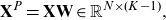
The classification results are shown in Figure 6, with each plot presenting the accuracies of the two approaches with a given value of n and all values of $\tau$
. For each plot, the horizontal axis represents the values of
$\tau$
. For each plot, the horizontal axis represents the values of $\tau$
, while the vertical axis represents the classification accuracy. The mean classification accuracies of the image recognition approach are shown by blue dashed curves while those of AIC are shown by red solid curves.
$\tau$
, while the vertical axis represents the classification accuracy. The mean classification accuracies of the image recognition approach are shown by blue dashed curves while those of AIC are shown by red solid curves.
Figure 6. Classification accuracies for fixed n and $\tau$
. The blue dashed curves represent the accuracies of the image recognition approach while the red solid curves represent those of AIC.
$\tau$
. The blue dashed curves represent the accuracies of the image recognition approach while the red solid curves represent those of AIC.
It is clear that, generally, the classification accuracy increases as $\tau$
increases for each value of n, and also increases as n increases for each value of
$\tau$
increases for each value of n, and also increases as n increases for each value of $\tau$
. This pattern makes sense because the underlying model can be better described by samples with larger n’s. The images generated with larger
$\tau$
. This pattern makes sense because the underlying model can be better described by samples with larger n’s. The images generated with larger $\tau$
’s are generally easier to classify, as the characteristics of the models are presented clearer when
$\tau$
’s are generally easier to classify, as the characteristics of the models are presented clearer when $\tau$
is larger. The image recognition approach can beat AIC when
$\tau$
is larger. The image recognition approach can beat AIC when $\tau$
is not high, that is less than 0.7, and this is more obvious when n is small. This is encouraging, as the improvement provided by the image recognition approach to select copula models occurs for samples that are difficult to classify, that is those with small n and
$\tau$
is not high, that is less than 0.7, and this is more obvious when n is small. This is encouraging, as the improvement provided by the image recognition approach to select copula models occurs for samples that are difficult to classify, that is those with small n and $\tau$
. However, when
$\tau$
. However, when $\tau$
is large, the image recognition approach performs apparently worse than AIC; moreover, beyond
$\tau$
is large, the image recognition approach performs apparently worse than AIC; moreover, beyond $\tau=0.7$
, the classification accuracies of the image recognition approach start decreasing. A plausible reason for this is that, when
$\tau=0.7$
, the classification accuracies of the image recognition approach start decreasing. A plausible reason for this is that, when $\tau$
is very large, the heatmap images of different copula models exhibit very similar visual patterns and image recognition cannot easily distinguish between them.
$\tau$
is very large, the heatmap images of different copula models exhibit very similar visual patterns and image recognition cannot easily distinguish between them.
To sum up, the preliminary experimental results on copula samples with fixed n and $\tau$
demonstrate the potential effectiveness of image recognition to select copula models, especially when n and
$\tau$
demonstrate the potential effectiveness of image recognition to select copula models, especially when n and $\tau$
are relatively small.
$\tau$
are relatively small.
Finally, we note that the design of the copula selection process proposed in this section entails some important decisions: the marginal distributions used for plotting heatmaps and the dimensions of the PC and LD subspaces. In the Supplementary Material (Appendix B.1), we provide robustness checks to evaluate the extent to which classification performance is impacted by such decisions.
4 Selecting rotated copula models
Encouraged by the results of Section 3, we here address the more realistic scenario where n and $\tau$
are not fixed. Furthermore, we allow
$\tau$
are not fixed. Furthermore, we allow $\tau$
to be negative. In particular, for asymmetric copula models, we consider all rotations, such that each model in
$\tau$
to be negative. In particular, for asymmetric copula models, we consider all rotations, such that each model in $\mathcal M_a$
has now four distinct versions. We believe that this addresses a realistic modelling scenario, as the classification approach does not assume anything a priori about the sign of either the correlation or the skewness of the underlying model.
$\mathcal M_a$
has now four distinct versions. We believe that this addresses a realistic modelling scenario, as the classification approach does not assume anything a priori about the sign of either the correlation or the skewness of the underlying model.
In this section, we consider three distinct approaches:
-
1. Copula selection with AIC. This approach requires us to consider an enlarged set of candidate models, which also includes the rotations of the positively correlated and skewed models in
$\mathcal M$
. -
2. Image recognition with a two-step approach. In the first step, sample statistics are used to assess the sign of correlation and skewness – essentially trying to detect if elements of
$\mathcal M$
have been rotated. Then, the pseudo-samples are transformed to have positive correlation and skewness. In the second step, heatmap images are generated from the transformed samples and classified to models in
$\mathcal M$
. -
3. Combining image recognition with AIC. The same approach as in 2. is followed, with the AIC of the models in
$\mathcal M$
added as a feature in the second step of the process. The motivation for this is to not miss out on any information encoded in likelihood-based statistical criteria, which is not present in image features.


The performance of the three copula model selection approaches is assessed on a test set. In contrast to Section 3, for the two-step approaches of this section we cannot validate the result of the classification algorithm on subsets of the training set. In the training set, all copula samples are positively correlated and skewed, to make the within-class variation smaller. However, this is not a realistic testing scenario. Thus, in the test set, we consider copula samples that may have negative or positive correlation and skewness. Before we discuss each of the three approaches in more depth, we describe the construction of this test set.
4.1 Test set
We produce two test sets of $S=10,000$
bivariate copula pseudo-samples: one with
$S=10,000$
bivariate copula pseudo-samples: one with $n \in [25,100]$
and the other with
$n \in [25,100]$
and the other with $n \in [100,250]$
, to test the classification performance of the copula selection methods on different ranges of sample sizes. These sample size ranges were chosen based on practical considerations. For sample sizes that are large, criteria such as AIC will lead to optimal model choices, which means that there is less scope for improvement from adding image features, as already glanced from Figure 6. If on the other hand sample sizes are very small, the model selection errors will be inescapably high, whichever method is used, and in such a situation a professional would typically prefer to use expert judgement. This leaves us with a ‘small-to-modest’ sample size range, for which improvements to standard model selection methods can be most meaningfully proposed. We consider that sample sizes from 25 to 250 give a suitable such range.
$n \in [100,250]$
, to test the classification performance of the copula selection methods on different ranges of sample sizes. These sample size ranges were chosen based on practical considerations. For sample sizes that are large, criteria such as AIC will lead to optimal model choices, which means that there is less scope for improvement from adding image features, as already glanced from Figure 6. If on the other hand sample sizes are very small, the model selection errors will be inescapably high, whichever method is used, and in such a situation a professional would typically prefer to use expert judgement. This leaves us with a ‘small-to-modest’ sample size range, for which improvements to standard model selection methods can be most meaningfully proposed. We consider that sample sizes from 25 to 250 give a suitable such range.
Each pseudo-sample is generated from a copula in $\mathcal M$
, with randomly (uniformly) chosen from the corresponding range of n and
$\mathcal M$
, with randomly (uniformly) chosen from the corresponding range of n and $\tau \in [0.1,0.9]$
. Before simulating each sample, the underlying copula model is rotated by 0, 90, 180, or 270 degrees counter-clockwise. Hence, we deal with an enlarged model set, denoted by
$\tau \in [0.1,0.9]$
. Before simulating each sample, the underlying copula model is rotated by 0, 90, 180, or 270 degrees counter-clockwise. Hence, we deal with an enlarged model set, denoted by $\mathcal M ^\prime$
. Let
$\mathcal M ^\prime$
. Let $m_{r}$
represent a model m in
$m_{r}$
represent a model m in $\mathcal M$
, rotated by r degrees, such that
$\mathcal M$
, rotated by r degrees, such that $m_0=m$
. For radially symmetric models
$m_0=m$
. For radially symmetric models $m\in \mathcal M_s$
, we also have
$m\in \mathcal M_s$
, we also have $m_{180}=m_0,\;m_{270}=m_{90}$
. Then, we let
$m_{180}=m_0,\;m_{270}=m_{90}$
. Then, we let $\mathcal M^\prime =\mathcal M^\prime_s \cup \mathcal M^\prime_a$
, where
$\mathcal M^\prime =\mathcal M^\prime_s \cup \mathcal M^\prime_a$
, where $M^\prime_s = \{m_r: \;m \in \mathcal M_s,\;r \in \{0,90\} \} $
and
$M^\prime_s = \{m_r: \;m \in \mathcal M_s,\;r \in \{0,90\} \} $
and $M^\prime_a = \big\{m_r: \;m \in \mathcal M_a,\;r \in \{0,90,180,270\}\big \} $
. The data and copula model specification are saved, as well as the rank correlation of the rotated model
$M^\prime_a = \big\{m_r: \;m \in \mathcal M_a,\;r \in \{0,90,180,270\}\big \} $
. The data and copula model specification are saved, as well as the rank correlation of the rotated model $\tau_r$
.
$\tau_r$
.
The process of generating the test set is given in detail in the Supplementary Material (Appendix C, Algorithm 2).
4.2 Copula selection approaches
4.2.1 Copula selection with AIC
For each instance i in the test set, the model in $\mathcal M^\prime$
with the smallest AIC is chosen. The classification is successful if the chosen model is identical to the underlying model
$\mathcal M^\prime$
with the smallest AIC is chosen. The classification is successful if the chosen model is identical to the underlying model $m_r\in \mathcal M^\prime $
.
$m_r\in \mathcal M^\prime $
.
4.2.2 Image recognition with a two-step approach
When we allow for models with negative correlation and skewness, the classification task becomes harder. One can either assign a different class for each element in the enlarged model space $\mathcal M^\prime$
– thus moving from 6 to 18 classes – or within each of the 6 classes in
$\mathcal M^\prime$
– thus moving from 6 to 18 classes – or within each of the 6 classes in $\mathcal M$
accommodate model rotations – resulting in non-homogeneous classes. We address this challenge pragmatically, by using the sample statistics
$\mathcal M$
accommodate model rotations – resulting in non-homogeneous classes. We address this challenge pragmatically, by using the sample statistics $\hat \tau,\;\hat \zeta$
to infer the rotation of the underlying model. Thus, as a first step pseudo-observations are transformed to have positive correlation and skewness. Subsequently, heatmap images are created from the transformed samples. As a second step, these heatmaps are classified, to select one of the 6 copula models in
$\hat \tau,\;\hat \zeta$
to infer the rotation of the underlying model. Thus, as a first step pseudo-observations are transformed to have positive correlation and skewness. Subsequently, heatmap images are created from the transformed samples. As a second step, these heatmaps are classified, to select one of the 6 copula models in $m \in \mathcal M$
. Thus in the image recognition stage we avoid the need to consider too many or very heterogeneous classes.
$m \in \mathcal M$
. Thus in the image recognition stage we avoid the need to consider too many or very heterogeneous classes.
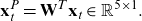
Figure 7 depicts the workflow of the two-step image recognition approach. The two steps are discussed in more detail below.
Figure 7. The workflow of the two-step approach for copula model selection.
Step 1 In order to arrive at homogeneous image classes, corresponding to the first step discussed above, samples are pre-processed as follows (the detailed algorithm is given in the Supplementary Material (Appendix C, Algorithm 3)). First we check whether the rank correlation is negative – if so the data are rotated by 90 degrees counter-clockwise. Then skewness is checked – if negative, the data are rotated by another 180 degrees. Let the quantity s represent the degree of data rotation to achieve a positive correlation and skewness; hence $\hat r=360-s$
is an estimate of the rotation r under which the pseudo-observations
$\hat r=360-s$
is an estimate of the rotation r under which the pseudo-observations $(u_j,v_j)$
were simulated. Sample statistics (including AIC values only used in the combined approach of Section 4.2.3) and images generated from the transformed sample and subsequently exported. The process is illustrated on the right of Figure 7, which shows an example of the heatmap image of a 90-degree rotated Pareto copula.
$(u_j,v_j)$
were simulated. Sample statistics (including AIC values only used in the combined approach of Section 4.2.3) and images generated from the transformed sample and subsequently exported. The process is illustrated on the right of Figure 7, which shows an example of the heatmap image of a 90-degree rotated Pareto copula.
Finally, we assess whether the first step has been performed successfully, in that the rotation applied to the data before producing the heatmap is consistent with the rotation of the underlying copula model. Radially symmetric and asymmetric models are treated differently, to reflect that for symmetric models $m_0=m_{180},\;m_{90}=m_{270}$
, which in practice requires us only to test whether the sign of the rank correlation
$m_0=m_{180},\;m_{90}=m_{270}$
, which in practice requires us only to test whether the sign of the rank correlation $\tau_r$
of the copula model
$\tau_r$
of the copula model $m_r$
matches that of the pseudo-observations,
$m_r$
matches that of the pseudo-observations, $\hat \tau$
.
$\hat \tau$
.
Step 2 In the second step, images generated by Step 1 are classified to models in $\mathcal M$
. The classification approach proceeds analogously with what was discussed in Section 3.2. The only difference is that, when generating a training sample of
$\mathcal M$
. The classification approach proceeds analogously with what was discussed in Section 3.2. The only difference is that, when generating a training sample of $R=20,000$
for each test set rather than using fixed n and
$R=20,000$
for each test set rather than using fixed n and $\tau$
as in Section 3.1, for each i these are now randomly chosen in the corresponding range of
$\tau$
as in Section 3.1, for each i these are now randomly chosen in the corresponding range of $n\in [25,100]$
or
$n\in [25,100]$
or $n\in [100,250]$
and
$n\in [100,250]$
and $\tau\in [0.1,0.9]$
. That is, predictions on each test set are performed based on the model trained on its corresponding training sample.
$\tau\in [0.1,0.9]$
. That is, predictions on each test set are performed based on the model trained on its corresponding training sample.
Once again we randomly split the $R= 20,000$
to a training set containing with 70% of the samples and a validation set with 30% of the samples. A SVM with RBF kernel is trained based on training sets of size
$R= 20,000$
to a training set containing with 70% of the samples and a validation set with 30% of the samples. A SVM with RBF kernel is trained based on training sets of size $0.7R=14,000$
. The training/validation split process is repeated 20 times.
$0.7R=14,000$
. The training/validation split process is repeated 20 times.
Finally, the 2-step approach is applied to classify the samples in the test set. For each test sample, we obtain 20 classification results based on the 20 classifiers trained in the training phase. A majority vote is applied to these results to get the final decision. In other words, the copula model with the highest vote by the 20 results is selected for the test copula sample.
We count a test sample as correctly classified only if both steps in the classification process are successful. In other words, for a sample to be classified correctly we need both to be true:
-
1. In the first step, the data were rotated in a way consistent with the underlying copula model.Footnote 5
-
2. In the second step, the classifier identifies the correct copula model out of the six models in
$\mathcal M$
. In other words, if the model underlying a test set was
$m_r \in \mathcal M^\prime$
, the prediction of the classifier is
$m \in \mathcal M$
.


Given the concurrent use of image-based and statistical features, it is of interest to consider which of those features drive the predictions of each model. A related sensitivity analysis, following the ideas of Pesenti et al. (Reference Pesenti, Millossovich and Tsanakas2019), is documented in the Supplementary Material (Appendix B.3).
4.2.3 Combining image recognition with AIC
The analysis of Section 3 has shown that image recognition and statistical approaches may be complementary, each being dominant in different ranges of n and $\tau$
. For that reason we propose to combine the two approaches. We adapt the approach of Section 4.2.2, to integrate AIC information for different models in
$\tau$
. For that reason we propose to combine the two approaches. We adapt the approach of Section 4.2.2, to integrate AIC information for different models in $\mathcal M$
in the second step of the process. Specifically:
$\mathcal M$
in the second step of the process. Specifically:
-
1. We follow the Step 1 of Section 4.2.2 in exactly the same way.
-
2. In Step 2, we follow again the approach of 4.2.2, but now adding the AIC values for
$l\in \mathcal M$
in both the training and testing phases. Specifically, for a training instance i denote the AIC values of different models by
$\mathbf{x}^A_i=\{\text{AIC}_i^{(l)}\}_{l \in \mathcal M}$
,
$i = 1,2,\ldots,N$
. The concatenated feature vector for each copula sample then becomes
$\mathbf{x}_i=[(\mathbf{x}^{MP}_i)^T,(\mathbf{x}^S_i)^T,(\mathbf{x}^A_i)^T]^T \in \mathbb{R}^{159 \times 1}$
. The rest of the training phase follows exactly as described in the second step of Section 4.2.2. Similarly, a test sample is represented by
$\mathbf{x}_t=[(\mathbf{x}^M_t)^T,(\mathbf{x}^S_t)^T,(\mathbf{x}^A_t)^T]^T \in \mathbb{R}^{159 \times 1}$
, where
$\mathbf{x}^A_t$
are the AIC values calculated for elements of
$\mathcal M$
, from the (rotated) data of the test set.
$\mathbf{x}_t$
is then projected to the linear discriminant subspace constructed in the training phase and classified by SVM.


4.2.4 Classification results
First we compare the performance of the different copula model selection methods presented in Section 4.2 by calculating their classification accuracies on the two test sets. The classification accuracies of the three approaches show similar patterns for both ranges of n. It is seen in Table 1 that the image recognition approach of Section 4.2.2 outperforms AIC. Furthermore, combining image recognition with AIC information, as in Section 4.2.3, leads to a better accuracy than either of those two approaches.
Table 1. Test classification accuracies of AIC, two-step image recognition approach, and combining image recognition with AIC.
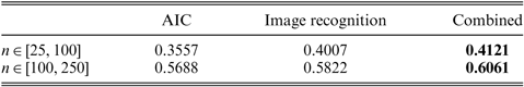
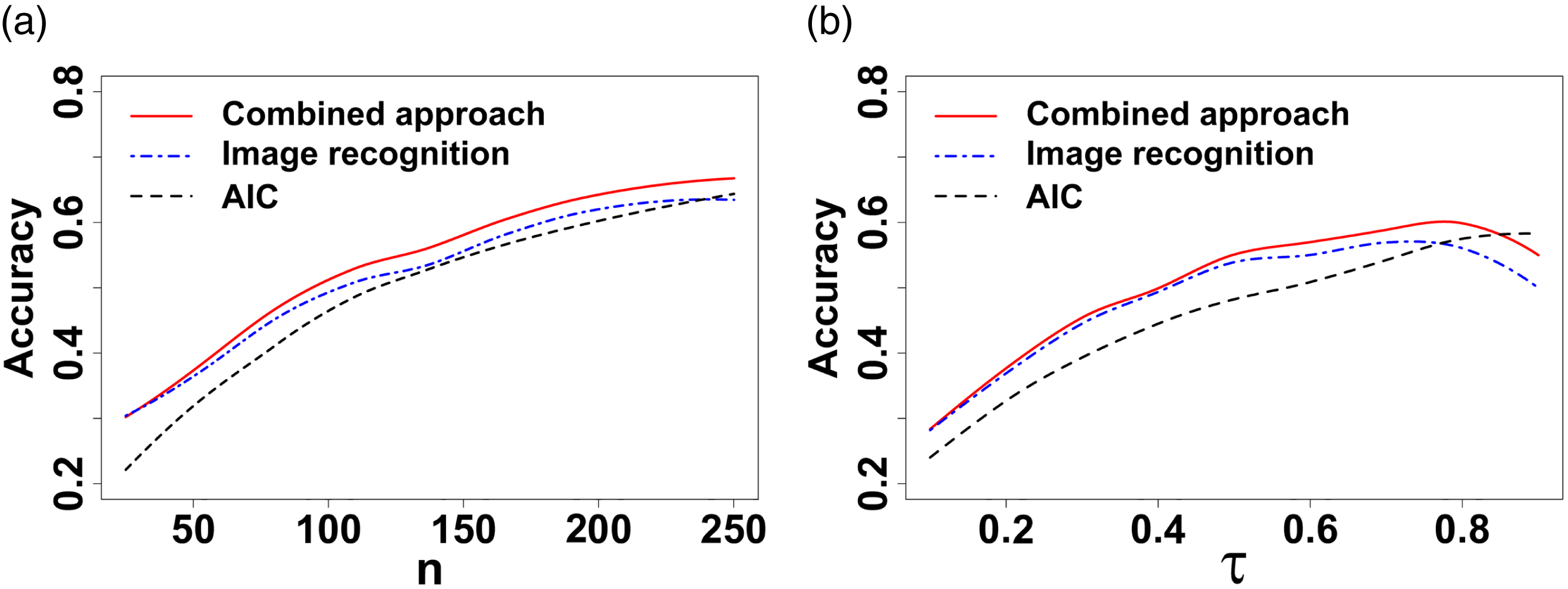
Figure 8. Fitted curves of the aggregated classification accuracies of the two test sets for the three approaches against (a) n and (b) $\tau$
.
$\tau$
.
To gain more insight into the test results, we plot smoothed curves of the average test classification accuracies of the three approaches against n and $\tau$
in Figure 8(a) and (b), respectively. Note that here we aggregate the results of both test sets to produce the two plots. The curves are generated by the function locfit of the package locfit with the smoothing parameter of
$\tau$
in Figure 8(a) and (b), respectively. Note that here we aggregate the results of both test sets to produce the two plots. The curves are generated by the function locfit of the package locfit with the smoothing parameter of $0.5$
. It is clear that the image recognition approach outperforms AIC, except for high correlations. Furthermore, the combined approach, including the information from both images and AIC, provides better results than simply using the image information in the two-step approach for all values of n and
$0.5$
. It is clear that the image recognition approach outperforms AIC, except for high correlations. Furthermore, the combined approach, including the information from both images and AIC, provides better results than simply using the image information in the two-step approach for all values of n and $\tau$
. Figure 8(a) shows that the combined approach is the best over all values of n while AIC is the worst, which is consistent with our conclusion in Table 1. However, Figure 8(b) presents a slightly different pattern for
$\tau$
. Figure 8(a) shows that the combined approach is the best over all values of n while AIC is the worst, which is consistent with our conclusion in Table 1. However, Figure 8(b) presents a slightly different pattern for $\tau$
: AIC performs better than both the combined and two-step approaches when the value of
$\tau$
: AIC performs better than both the combined and two-step approaches when the value of $\tau$
is larger than 0.9. This indicates that the heatmap image information does not help copula selection when
$\tau$
is larger than 0.9. This indicates that the heatmap image information does not help copula selection when $\tau$
is very high.
$\tau$
is very high.
Table 2. Confusion matrix of the approach combining image recognition and AIC on the two test sets.

Table 3. Confusion matrix of the two-step image recognition approach on the two test sets.
In Tables 2 and 3, respectively, we present the confusion matrices of the image recognition and combined approaches by aggregating the results of the two test sets. The classification accuracies for each class are summarised in the bottoms of each table. For simplicity of exposition, we calculate the confusion matrices only for those testing instances where we had $FirstStep=$
TRUE (99.02% of instances). It is apparent that the Frank, Gaussian and Joe models are best predicted. Predictions for underlying Gumbel and t models are less accurate, while for Pareto models the predictions are the worst. Pareto models are confused with Joe by both approaches, due to the similarity between their heatmap images. Comparing Tables 2 and 3, we can see that the combined approach can provide better predictions across all models (with only a small drop in accuracy for Joe), which demonstrates the effectiveness of involving the information provided by AIC.
$FirstStep=$
TRUE (99.02% of instances). It is apparent that the Frank, Gaussian and Joe models are best predicted. Predictions for underlying Gumbel and t models are less accurate, while for Pareto models the predictions are the worst. Pareto models are confused with Joe by both approaches, due to the similarity between their heatmap images. Comparing Tables 2 and 3, we can see that the combined approach can provide better predictions across all models (with only a small drop in accuracy for Joe), which demonstrates the effectiveness of involving the information provided by AIC.
Based on this analysis, we find that image recognition offers improvements in the accuracy of bivariate copula model selection, when compared to using the AIC benchmark. Furthermore, combining those two is best and we consider this combined approach our preferred model. Further supporting evidence is given in the Supplementary Material (Appendix B.2), where the impact of using purely statistical or image features is explored.
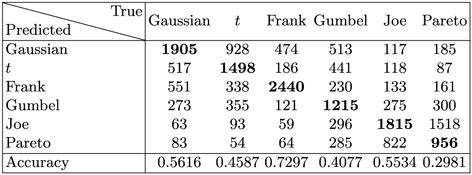
Figure 9. (a) Scatter plot of weekly log-losses for the MSCI (ticker: ‘NDDUWI’) and RISX (ticker: ‘RISXNTR’) indices (10/01/2020 – 31/12/2021); (b) smoothed bivariate density heatmap (normal marginals).

Figure 10. (a) Development of the MSCI (ticker: ‘NDDUWI’) and RISX (ticker: ‘RISXNTR’) indices (06/2006 – 12/2021); (b) rank correlation between weekly log-losses, with a 2-year rolling window. The colour indicates the copula model selected.

Figure 11. Predicted probabilities for different types of copula model; darker colours indicate models with more (right) tail risk.
5 Real data application
Here, we apply the copula selection framework developed in the paper to modelling (unconditional) joint weekly net total returns – that is, including dividends reinvested net of withholding taxes – of the MSCI World Index (ticker: ‘NDDUWI’) and the ICMR (Re)Insurance Specialty Index (ticker: ‘RISXNTR’) (both in USD). The MSCI World Index is a market capitalisation weighted index representing equity performance across developed markets (MSCI 2022). RISX is an equity-based benchmark for the global specialty (re)insurance sector, based on publicly listed companies that underwrite risks in the Lloyd’s of London market (Insurance Capital Markets Research 2022). Modelling the dependence between those two indices reflects diversification considerations that are important for investment decisions and for insurance operations. In particular, a lower level of correlation between global equity markets and the (re)insurance industry makes the latter attractive for investors, which has a direct impact on insurers’ capital availability and, by implication, competition and commercial premium rates.
We consider the dependence structure of the weekly log-losses (negative log-returns) of the two indices. First, we select a copula model for the 104 joint observations from 10/01/2020 – 31/12/2021, hence covering an approximate 2-year period. In Figure 9(a), we show the scatter plot of weekly log-losses from the two indices; in Figure 9(b), as in previous sections, we represent the dependence structure by a smoothed density heatmap, after transforming the marginals to normal. The substantial correlation between the returns ( $\hat\tau=0.5878$
) is apparent. Furthermore, we have sample skewness and arachnitude of
$\hat\tau=0.5878$
) is apparent. Furthermore, we have sample skewness and arachnitude of $\hat\zeta=0.0007$
(indicating near symmetry) and
$\hat\zeta=0.0007$
(indicating near symmetry) and $\hat\xi=0.6271$
, respectively. Using those statistics and Figure 9(b), we select a copula model using the combined approach of Section 4.2.3. A t model is chosen, with fitted degree-of-freedom parameter
$\hat\xi=0.6271$
, respectively. Using those statistics and Figure 9(b), we select a copula model using the combined approach of Section 4.2.3. A t model is chosen, with fitted degree-of-freedom parameter $\hat\nu=5.064$
.
$\hat\nu=5.064$
.
We now examine changes in the dependence structure of weekly log-losses over a longer time period. We use data from 16/06/2006 – 31/12/2021 (811 observations), hence reflecting the impacts of both the 2007–2008 global financial crisis and the 2020(-present) COVID-19 pandemic. First, in Figure 10(a), we plot the development of the two indices over time, normalised to have the same starting point – the joint drop in early 2020 and subsequent recovery are clearly visible. In Figure 10(b), we show the path of Kendall’s $\tau$
for the weekly log-losses, calculated with a 104-week (2-year) rolling window. It is seen that correlation has changed over time, with a more or less continuous drop during 2011–2019, and a subsequent increase (one cannot attribute this increase to COVID-19, as it had started already before 2020). On the same plot, we also indicate the chosen copula family using the combined approach of Section 4.2.3. It is seen that there are some changes in the selected model over time. The most frequently selected model is the t copula (red squares). Early in the series, the Gumbel copula (blue triangles) is also commonly selected. Furthermore, the Gaussian copula (green circles) seems to often be chosen during periods when the correlation value is on a decreasing trajectory. Other models appear less frequently; it is notable that occasionally the (180-degree-)rotated Gumbel copula (magenta crosses) is chosen, reflecting a benign scenario where the dependence of log-losses is negatively skewed. Overall, this analysis provides strong evidence for non-stationary of the dependence structure (and not just the correlation) of the two indices.
$\tau$
for the weekly log-losses, calculated with a 104-week (2-year) rolling window. It is seen that correlation has changed over time, with a more or less continuous drop during 2011–2019, and a subsequent increase (one cannot attribute this increase to COVID-19, as it had started already before 2020). On the same plot, we also indicate the chosen copula family using the combined approach of Section 4.2.3. It is seen that there are some changes in the selected model over time. The most frequently selected model is the t copula (red squares). Early in the series, the Gumbel copula (blue triangles) is also commonly selected. Furthermore, the Gaussian copula (green circles) seems to often be chosen during periods when the correlation value is on a decreasing trajectory. Other models appear less frequently; it is notable that occasionally the (180-degree-)rotated Gumbel copula (magenta crosses) is chosen, reflecting a benign scenario where the dependence of log-losses is negatively skewed. Overall, this analysis provides strong evidence for non-stationary of the dependence structure (and not just the correlation) of the two indices.
The SVM-based classifiers allow us to state not just the chosen model, but also predicted probabilities for each model considered. We visualise these predicted probabilities in the stacked area plot of Figure 11. To aid interpretability, we now group the selected copula models in four categories, from the most adverse (darkest) to the least adverse (lightest): positively skewed (Gumbel, Pareto, Joe); symmetric and tail dependent (t); symmetric and tail independent (Gaussian, Frank); and negatively skewed (rotated Gumbel, Pareto, Joe). Hence, during time periods when the dark greys dominate, a more adverse dependence structure is present. From that perspective, it appears that we have adverse dependence regimes during 2008–2014 and from 2019 to the present. The extent to which these trends can be associated to phenomena such as insurance cycles remains a topic for further work.
6 Conclusions
In this paper, we proposed approaches for selecting copula models by utilising image recognition of the density heatmap images obtained from copula samples. PCA-reduced AlexNet image features and summary statistics were utilised to represent each copula sample and a low-dimensional discriminative projection by LDA used to train an SVM for classification. Experimental results showed that the proposed image recognition approach can provide improved classification performance on copula samples with relatively low sample size and correlation, compared to AIC. When combining image recognition with AIC, performance improves further.
Hence, we can answer our research question in the affirmative: indeed, heatmap images do contain relevant information for copula model selection that can help improve on standard procedures, and we propose workflows to harness this information for model selection. Furthermore, we demonstrate the potential value of transfer learning in statistical applications. In this paper, the knowledge obtained from the domain of natural images is transferred to the different domain of copula heatmap images, to assist in the new classification task of copula selection. This shows the potential of utilising machine learning algorithms that have been trained on a large amount of high-quality data to provide additional useful information for statistical applications, or to help in situations where collecting enough data is not an easy task (Pan and Yang Reference Pan and Yang2009).
The workflows we propose are more complex than evaluating likelihood-based criteria, at least where efficient implementation of the latter is available. We do not argue for replacing well-established criteria such as AIC, but provide a ‘proof of concept’ that image recognition can supplement standard statistical approaches. With this in mind, future work can consider designing an expert system with a broader scope, for example including a wider range of models and sample sizes, as well as handling multivariate dependence structures. For example, one may consider (partially) representing a copula sample with multivariate dependence structure, via two-dimensional heatmap images generated from pairwise bivariate dependence structures. In this way, each sample is represented by a set of images, which leads to the image set classification task in computer vision (Fukui and Maki Reference Fukui and Maki2015).
Supplementary material
To view supplementary material for this article, please visit http://doi.org/10.1017/asb.2022.12.


 Open access