


I. INTRODUCTION
The technique of blind source separation (BSS) has been studied for decades [Reference Jutten and Herault1–Reference Makino, Lee and Sawada5], and the research is still in progress. The term “blind” refers to the situation that the source activities and the mixing system information are unknown. There are many diverse purposes for developing this technology even if audio signals are focused on, such as (1) implementing the cocktail party effect as an artificial intelligence, (2) extracting the target speech in a noisy environment for better speech recognition results, (3) separating each musical instrumental part of an orchestra performance for music analysis.
Various signal processing and machine learning methods have been proposed for BSS. They can be classified using two axes (Fig. 1). The horizontal axis relates to the number M of microphones used to observe sound mixtures. The most critical distinction is whether M=1 or M ≥ 2, i.e., a single-channel or multichannel case. In a multichannel case, the spatial information of a source signal (e.g., source position) can be utilized as an important cue for separation. The second critical distinction is whether the number M of microphones is greater than or equal to the number N of source signals. In determined (N=M) and overdetermined (N<M) cases, the separation can be achieved using linear filters. For underdetermined (N>M) cases, one popular approach is based on clustering, such as by the Gaussian mixture model (GMM), followed by time-frequency masking [Reference Jourjine, Rickard and Yilmaz6–Reference Ito, Araki and Nakatani12]. The vertical axis indicates whether training data are utilized or not. If so, the characteristics of speech and audio signals can be learned beforehand. The learned knowledge helps to optimize the separation system, especially for single-channel cases where no spatial cues can be utilized. Recently, many methods based on deep neural networks (DNNs) have been proposed [Reference Hershey, Chen, Le Roux and Watanabe13–Reference Leglaive, Girin and Horaud21].
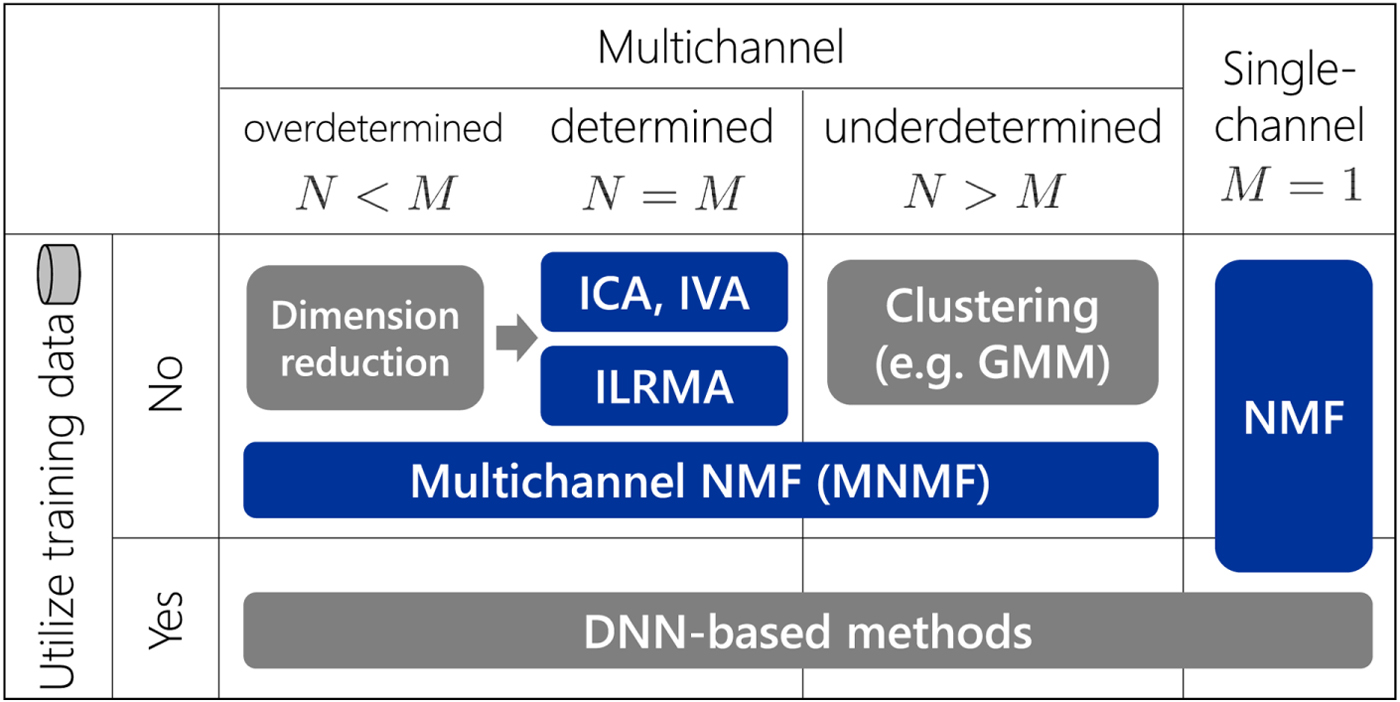
Fig. 1. Various methods for blind audio source separation. Methods in blue are discussed in this paper in an integrated manner.
Among the various methods shown in Fig. 1, this paper discusses the methods in blue. The motivation for selecting these methods is twofold: (1) As shown in Fig. 2, two originally different methods, independent component analysis (ICA) [Reference Hyvärinen, Karhunen and Oja3,Reference Cichocki and Amari4,Reference Comon22–Reference Ono and Miyabe29] and nonnegative matrix factorization (NMF) [Reference Lee and Seung30–Reference Févotte and Idier36], have historically been extended to independent vector analysis (IVA) [Reference Hiroe37–Reference Ikeshita, Kawaguchi, Togami, Fujita and Nagamatsu46] and multichannel NMF [Reference Ozerov and Févotte47–Reference Kameoka, Sawada, Higuchi and Makino54], respectively, which have recently been unified as independent low-rank matrix analysis (ILRMA) [Reference Kameoka, Yoshioka, Hamamura, Le Roux and Kashino55–Reference Mogami60]. (2) The objective functions used in these methods can effectively be minimized by majorization-minimization algorithms with appropriately designed auxiliary functions [Reference Févotte and Idier36,Reference Lange, Hunter and Yang61–Reference Sun, Babu and Palomar68]. With regard to these two aspects, all the selected methods are related and worth explaining in a single review paper.
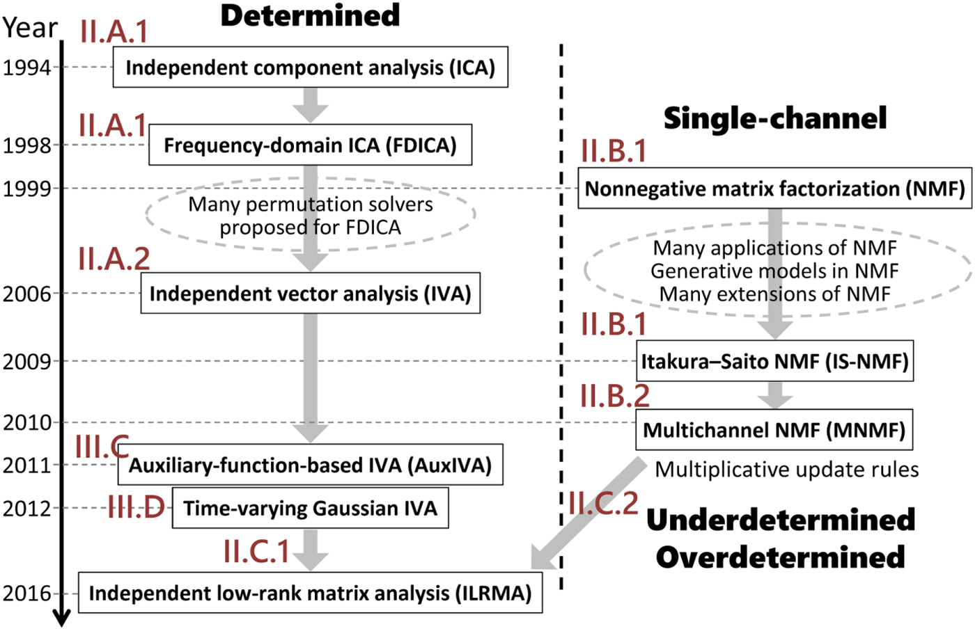
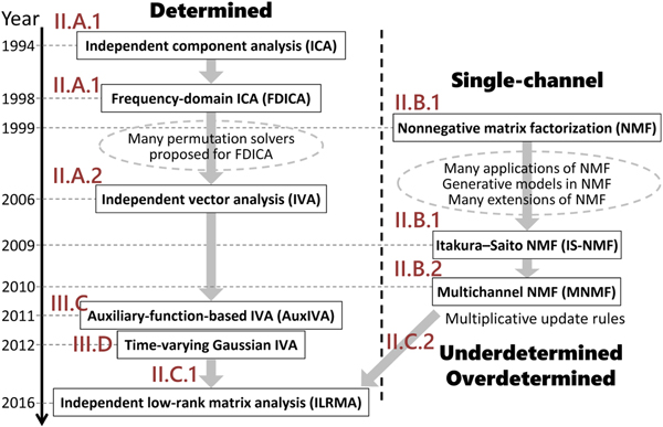
Fig. 2. Historical development of BSS methods.
Although the mixing situation is unknown in the BSS problem, the mixing model is described as follows. Let s 1, …, s N be N original sources and x 1, …, x M be M mixtures at microphones. Let h mn denote the transfer characteristic from source s n to mixture x m. When h mn is described by a scalar, the problem is called instantaneous BSS and the mixtures are modeled as
 $$x_m(t) = \sum_{n=1}^N h_{mn} s_n(t), \quad m=1, \ldots, M, $$
where t represents time. When h mn is described by an impulse response of L samples that represents the delay and reverberations in a real-room situation, the problem is called convolutive BSS and the mixtures are modeled as
 $$x_m(t) = \sum_{n=1}^N \sum_{\tau=0}^{L-1} h_{mn}(\tau) s_n(t-\tau), \quad m=1,\ldots, M.$$
To cope with a real-room situation, we need to solve the convolutive BSS problem.
Although there have been proposed time-domain approaches [Reference Amari, Douglas, Cichocki and Yang69–Reference Koldovsky and Tichavsky75] to the convolutive BSS problem, a more suitable approach for combining ICA and NMF is a frequency-domain approach [Reference Smaragdis76–Reference Duong, Vincent and Gribonval85], where we apply a short-time Fourier transformation (STFT) to the time-domain mixtures (2). Using a sufficiently long STFT window to cover the main part of the impulse responses, the convolutive mixing model (2) can be approximated with the instantaneous mixing model
 $$x_{ij,m} = \sum_{n=1}^N h_{i,mn} s_{ij,n}, \quad m=1,\ldots, M$$
in each frequency bin i, with time frame j representing the position index of each STFT window. Table 1 summarizes the notations used in this paper.
Table 1. Notations.
The data structure that we deal with is a complex-valued tensor with three axes, frequency i, time j, and channel (mixture m or source n), as shown on the left-hand side of Fig. 3. Until IVA was invented in 2006, there had been no clear way to handle the tensor in a unified manner. A practical way was to slice the tensor into frequency-dependent matrices with time and channel axes, and apply ICA to the matrices. Another historical path is from NMF, applied to a matrix with time and frequency axes, to multichannel NMF. These two historical paths merged with the invention of ILRMA, as shown in Figs 2 and 3.
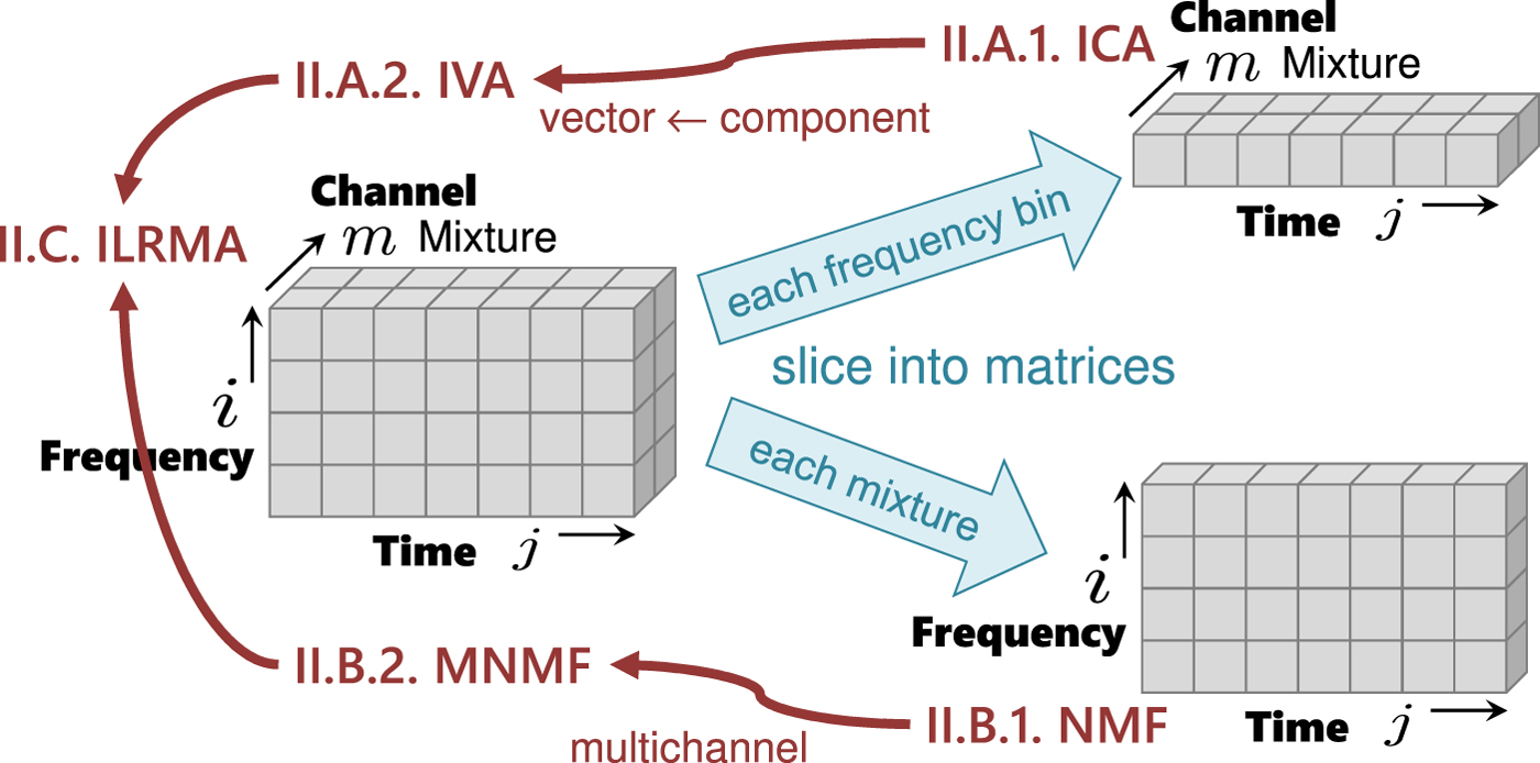
Fig. 3. Tensor and sliced matrices.
The rest of the paper is organized as follows. In Section II, we introduce probabilistic models for all the above methods and define corresponding objective functions. In Section III, we explain how to optimize the objective functions based on majorization-minimization by designing auxiliary functions. Section IV shows illustrative experimental results to provide an intuitive understanding of the characteristics of all these methods. Section V concludes the paper.
II. MODELS
A) ICA and IVA
In this subsection, we assume determined (N=M) cases for the application of ICA and IVA. For overdetermined (N<M) cases, we typically apply a dimension reduction method such as principal component analysis to the microphone observations as a preprocessing [Reference Winter, Sawada and Makino86,Reference Osterwise and Grant87].
1) ICA
Let the sliced matrix depicted in the upper right of Fig. 3 be  ${\bf X}_i = \{{\bf x}_{ij}\}_{j=1}^J$ with xij = [x ij,1, …, x ij,M]T. ICA calculates an M-dimensional square separation matrix Wi that linearly transforms the mixtures xij to source estimates yij = [y ij,1, …, y ij,N]T by
 $${\bf y}_{ij} = {\bf W}_i\,{\bf x}_{ij}.$$
The separation matrix Wi can be optimized in a maximum likelihood sense [Reference Cardoso26]. We assume that the likelihood of Wi is decomposed into time samples
 $$p({\bf X}_i \vert {\bf W}_i) = \prod_{j=1}^J p({\bf x}_{ij}\vert {\bf W}_i).$$
The complex-valued linear operation (4) transforms the density as
 $$p({\bf x}_{ij}\vert {\bf W}_i) = \vert {\rm det}\,{\bf W}_i\vert^2\, p({\bf y}_{ij}).$$
We assume that the source estimates are independent of each other,
 $$p({\bf y}_{ij}) = \prod_{n=1}^N p(y_{ij,n}).$$
Putting (5)–(7) together, the negative log-likelihood  ${\cal C} ({\bf W}_i) = -\log p({\bf X}_i\vert {\bf W}_i)$, as the objective function to be minimized, is given by
 $${\cal C}({\bf W}_i) = \sum_{j=1}^J\sum_{n=1}^N G(y_{ij,n}) -2J\log \vert {\rm det}\,{\bf W}_i\vert,$$
where G(y ij,n) = −log p(y ij,n) is called a contrast function. In speech/audio applications, a typical choice for the density function is the super-Gaussian distribution
 $$p(y_{ij,n}) \propto \exp \left( -\displaystyle{\sqrt{\vert y_{ij,n}\vert ^2+\alpha} \over \beta}\right),$$
with nonnegative parameters α and β. How to minimize the objective function (8) will be explained in Section III.
By applying ICA to the every sliced matrix, we have N source estimates for every frequency bin. However, the order of the N source estimates in each frequency bin is arbitrary, and therefore we have the so-called permutation problem. One approach to this problem is to align the permutations in a post-processing [Reference Sawada, Araki and Makino11,Reference Sawada, Mukai, Araki and Makino88]. This paper focuses on tensor methods (IVA and ILRMA) as another approach that automatically solves the permutation problem.
2) IVA
Figure 4 shows the difference between ICA and IVA. In ICA, we assume the independence of scalar variables, e.g., y ij,1 and y ij,2. In IVA, the notion of independence is extended to vector variables. Let us define a vector of source estimates spanning all frequency bins as  ${\bf y}_{j,n} = [y_{1j,n},\ldots ,y_{Ij,n}]^{\ssf T}$. The independence among source estimate vectors is expressed as
 $$p(\{{\bf y}_{j,n}\}_{n=1}^N) = \prod_{n=1}^N p({\bf y}_{j,n}) .$$
We now focus on the left-hand side of Fig. 3. The mixture is denoted by two types of vectors. The first one is channel-wise  ${\bf x}_{ij} = [x_{ij,1},\ldots , x_{ij,M}]^{\ssf T}$. The second one is frequency-wise ${\bf x}_{j,m} = [x_{1j,m},\ldots ,x_{Ij,m}]^{\ssf T}$. The source estimates are calculated by (4) using the first type for all frequency bins i = 1, …, I. A density transformation similar to (6) is expressed using the second type as follows:
 $$p(\{{\bf x}_{j,m}\}_{m=1}^M\vert {\cal W}) = p(\{{\bf y}_{j,n}\}_{n=1}^N) \prod_{i=1}^I \vert {\rm det}\,{\bf W}_i\vert ^2,$$
with  ${\cal W} = \{{\bf W}_i\}_{i=1}^I$ being the set of separation matrices of all frequency bins. Similarly to (5), the likelihood of ${\cal W}$ is decomposed into time samples as
 $$p({\cal X}\vert {\cal W}) = \prod_{j=1}^J p(\{{\bf x}_{j,m}\}_{m=1}^M\vert {\cal W}),$$
where  ${\cal X} = \{\{{\bf x}_{j,m}\}_{m=1}^M\}_{j=1}^J$. Putting (10)–(12), together, the objective function, i.e., the negative log-likelihood, ${\cal C} ({\cal W}) = -\log p({\cal X}\vert {\cal W})$ is given as
 $${\cal C} ({\cal W}) = \sum_{j=1}^J\sum_{n=1}^N G({\bf y}_{j,n}) -2J\sum_{i=1}^I\log \vert {\rm det}\,{\bf W}_i\vert,$$
where G(yj,n) = −log p(yj,n) is again a contrast function. A typical choice for the density function is the spherical super-Gaussian distribution
 $$p({\bf y}_{j,n}) \propto \exp\left(- \displaystyle{\sqrt{\sum_{i=1}^I \vert y_{ij,n}\vert ^2+\alpha}\over \beta} \right),$$
with nonnegative parameters α and β. How to minimize the objective function (13) will be explained in Section III.

Fig. 4. Independence in ICA and IVA.
Comparing (9) and (14), we see that there are frequency dependences in the IVA cases. These dependences contribute to solving the permutation problem.
B) NMF and MNMF
Generally, NMF objective functions are defined as the distances or divergences between an observed matrix and a low-rank matrix. Popular distance/divergence measures are the Euclidean distance [Reference Lee and Seung31], the generalized Kullback–Leibler (KL) divergence [Reference Lee and Seung31], and the Itakura–Saito (IS) divergence [Reference Févotte, Bertin and Durrieu33]. In this paper, aiming to clarify the connection of NMF to IVA and ILRMA, we discuss NMF with the IS divergence (IS-NMF).
1) NMF
Let the sliced matrix depicted in the lower right of Fig. 3 be X, [X]ij = x ij. Microphone index m is omitted here for simplicity. The nonnegative values considered in IS-NMF are the power spectrograms |x ij|2, and they are approximated with the rank K structure
 $$ \vert x_{ij}\vert ^2 \approx \sum_{k=1}^K t_{ik}v_{kj} = \hat{x}_{ij},$$
with nonnegative matrices T, [T]ik = t ik, and V, [V]kj = v kj, for i = 1, …, I and j = 1, …, J. In a matrix notation, we have
 $${\bf X} = {\bf TV},$$
as a matrix factorization form. Figure 5 shows that a spectrogram can be modeled with this NMF model.
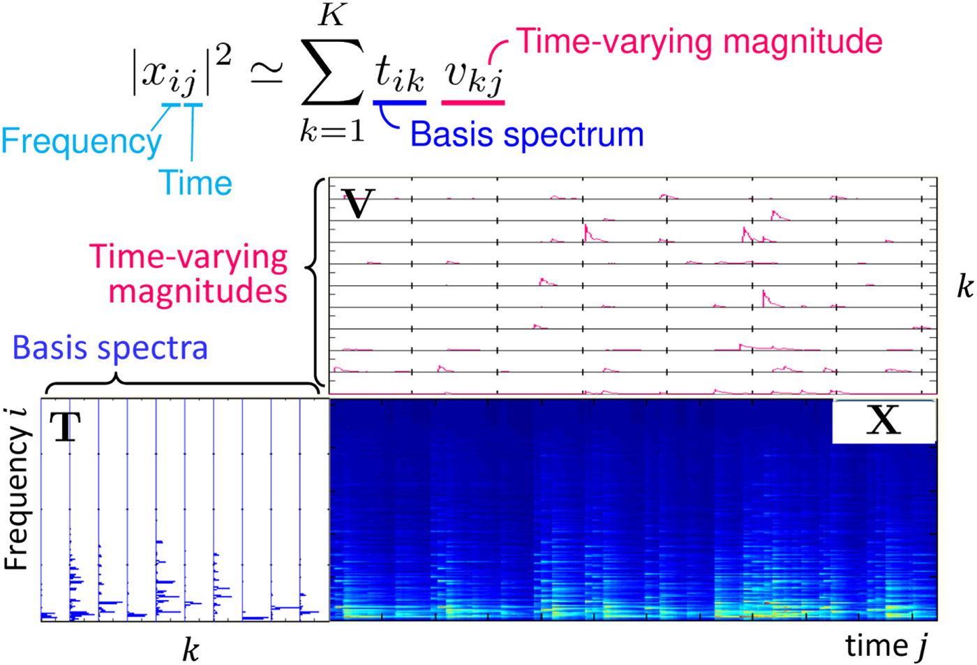
Fig. 5. NMF as spectrogram model fitting.
The objective function of IS-NMF can be derived in a maximum-likelihood sense. We assume that the likelihood of T and V for X is decomposed into matrix elements
 $$ p({\bf X}\vert {\bf T},{\bf V}) = \prod_{i=1}^I\prod_{j=1}^J p(x_{ij}\vert \hat{x}_{ij}),$$
and each element x ij follows a zero-mean complex Gaussian distribution with variance  $\hat{x}_{ij}$ defined in (15),
 $$ p(x_{ij}\vert \hat{x}_{ij}) \propto \displaystyle{1 \over \hat{x}_{ij}}\exp \left(-\displaystyle{\vert x_{ij}\vert ^2 \over \hat{x}_{ij}}\right).$$
Then, the objective function  ${\cal C} ({\bf T},{\bf V}) = -\log p({\bf X}\vert {\bf T},{\bf V})$ is simply given as
 $$ {\cal C}({\bf T},{\bf V}) = \sum_{i=1}^I\sum_{j=1}^J \left[ \displaystyle{\vert x_{ij}\vert ^2 \over \hat{x}_{ij}} + \log\hat{x}_{ij} \right].$$
The IS divergence between |x ij|2 and  $\hat{x}_{ij}$ is defined as [Reference Févotte, Bertin and Durrieu33]
 $$d_{IS}(\vert x_{ij}\vert ^2, \hat{x}_{ij}) = \displaystyle{\vert x_{ij}\vert ^2 \over \hat{x}_{ij}} - \log \displaystyle{\vert x_{ij}\vert ^2 \over \hat{x}_{ij}} - 1 ,$$
and is equivalent to the ij-element of the objective function (19) up to a constant term. How to minimize the objective function (19) will be explained in Section III.
2) MNMF
We now return to the left-hand side of Fig. 3 from the lower-right corner, and the scalar x ij,m is extended to the channel-wise vector  ${\bf x}_{ij} = [x_{ij,1},\ldots ,x_{ij,M}]^{\ssf T}$. The power spectrograms |x ij|2 considered in NMF are now extended to the outer product of the channel vector
 $$ {\ssf X}_{ij} = {\bf x}_{ij}{\bf x}^{\ssf H}_{ij} = \left[\matrix{\vert x_{ij,1}\vert ^2 & \ldots & \!\! x_{ij,1}x_{ij,M}^{\ast} \cr \vdots & \ddots & \vdots \cr x_{ij,M}x_{ij,1}^{\ast} \!\! & \ldots & \vert x_{ij,M}\vert ^2}\right].$$
To build a multichannel NMF model, let us introduce a Hermitian positive semidefinite matrix  ${\ssf H}_{ik}$ that is the same size as ${\ssf X}_{ij}$ and models the spatial property [Reference Arberet48,Reference Sawada, Kameoka, Araki and Ueda49,Reference Vincent, Jafari, Abdallah, Plumbley, Davies and Wang84,Reference Duong, Vincent and Gribonval85] of the kth NMF basis in the ith frequency bin. Then, the outer products are approximated with a rank-K structure similar to (15),
 $$ {\ssf X}_{ij} \approx \sum_{k=1}^K {\ssf H}_{ik}t_{ik}v_{kj} = \hat{\ssf X}_{ij} .$$
 The objective function of MNMF can basically be defined as the total sum  $\sum _{i=1}^I \sum _{j=1}^J d_{IS}({\ssf X}_{ij}, \hat{\ssf X}_{ij})$ of the multichannel IS divergence (see [Reference Sawada, Kameoka, Araki and Ueda49] for the definition) between ${\ssf X}_{ij}$ and $\hat{\ssf X}_{ij}$, and can also be derived in a maximum-likelihood sense. Let $\underline{\bf H}$ be an I × K hierarchical matrix such that $[\underline{\bf H}]_{ik} = {\ssf H}_{ik}$. We assume that the likelihood of T, V, and $\underline{\bf H}$ for ${\cal X} = \{\{{\bf x}_{ij}\}_{i=1}^I\}_{j=1}^J$ is decomposed as
 $$ p({\cal X}\vert {\bf T},{\bf V},\underline{\bf H}) = \prod_{i=1}^I\prod_{j=1}^J p({\bf x}_{ij}\vert \hat{\ssf X}_{ij}),$$
and that each vector xij follows a zero-mean multivariate complex Gaussian distribution with the covariance matrix  $\hat{\ssf X}_{ij}$ defined in (22),
 $$p({\bf x}_{ij}\vert \hat{\ssf X}_{ij}) \propto \displaystyle{1 \over {\rm det}\hat{\ssf X}_{ij}}\exp \left(- {\bf x}_{ij}^{\ssf H}\hat{\ssf X}_{ij}^{-1}{\bf x}_{ij}\right).$$
Then, similar to (19), the objective function  ${\cal C} ({\bf T},{\bf V},\underline{\bf H}) = -\log p({\cal X}\vert {\bf T},{\bf V},\underline{\bf H})$ is given as
 $${\cal C}({\bf T},{\bf V},\underline{\bf H}) = \sum_{i=1}^I\sum_{j=1}^J \left[ {\bf x}_{ij}^{\ssf H}\hat{\ssf X}_{ij}^{-1}{\bf x}_{ij} + \log {\rm det}\hat{\ssf X}_{ij} \right].$$
How to minimize the objective function (25) will be explained in Section III.
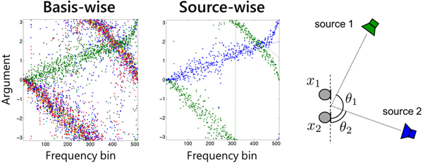
The spatial properties  ${\ssf H}_{ik}$ learned by the model (22) can be used as spatial cues for clustering NMF bases. In particular, the argument $\arg ([{\ssf H}_{ik}]_{mm'})$ of an off-diagonal element m ≠ m′ represents the phase difference between the two microphones m and m′. The left plot of Fig. 6 follows model (22) with k = 1, …, 10. The 10 bases can be clustered into two sources based on their arguments as a post-processing. However, a more elegant way is to introduce the cluster-assignment variable [Reference Ozerov, Févotte, Blouet and Durrieu89] z kn ≥ 0, $\sum _{n=1}^N z_{kn}=1$, k = 1, …, K, n = 1, …, N, and the source-wise spatial property ${\ssf H}_{in}$, and express the basis-wise property as ${\ssf H}_{ik} = \sum _{n=1}^N z_{kn}{\ssf H}_{in}$. As a result, the model (22) and the objective function (25) respectively become
 $$\hat{\ssf X}_{ij} = \sum_{k=1}^K \sum_{n=1}^N z_{kn}{\ssf H}_{in}t_{ik}v_{kj},$$
 $${\cal C}({\bf T},{\bf V},\underline{\bf H},{\bf Z}) = \sum_{i=1}^I\sum_{j=1}^J \left[ {\bf x}_{ij}^{\ssf H}\hat{\ssf X}_{ij}^{-1}{\bf x}_{ij} + \log{\rm det}\hat{\ssf X}_{ij}, \right]$$
with [Z]kn = z kn and the size of  $\underline{\bf H}$ being I × N. The middle plot of Fig. 6 shows the result following the model (26). We see that source-wise spatial properties are successfully learned. The objective function (27) can be minimized in a similar manner to (25).
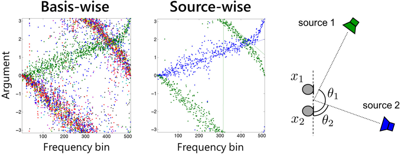
Fig. 6. Example of MNMF-learned spatial property. The left and middle plots show the learned complex arguments  ${\rm arg}([{\ssf H}_{ik}]_{12}), k=1,\ldots,10$, and ${\rm arg}([{\ssf H}_{in}]_{12}), n=1,2$, respectively. The right figure illustrates the corresponding two-source two-microphone situation.
C) ILRMA
ILRMA can be explained in two ways, as there are two paths in Fig. 2.
1) Extending IVA with NMF
The first way is to extend IVA by introducing NMF for source estimates, as illustrated in Fig. 7, with the aim of developing more precise spectral models. Let the objective function (13) of IVA be rewritten as
 $${\cal C}({\cal W}) = \sum_{n=1}^N G({\bf Y}_{n}) -2J\sum_{i=1}^I\log \vert {\rm det}\,{\bf W}_i\vert$$
with Yn being an I × J matrix, [Yn]ij = y ij,n. Then, let us introduce the NMF model for Yn as
 $$p({\bf Y}_{n}\vert {\bf T}_n,{\bf V}_n) = \prod_{i=1}^I \prod_{j=1}^J p(y_{ij,n}\vert \hat{y}_{ij,n})$$
 $$p(y_{ij,n}\vert \hat{y}_{ij,n}) \propto \displaystyle{1 \over \hat{y}_{ij,n}}\exp\left( -\displaystyle{\vert y_{ij,n}\vert ^2 \over \hat{y}_{ij,n}} \right)$$
 $$\hat{y}_{ij,n} =\sum_{k=1}^K t_{ik,n}v_{kj,n}$$
with [Tn]ik = t ik,n and [Vn]kj = v kj,n. The objective function is then
 $$\eqalign{{\cal C}({\cal W},\{{\bf T}_n\}_{n=1}^N, \{{\bf V}_n\}_{n=1}^N) &=\sum_{n=1}^N\sum_{i=1}^I\sum_{j=1}^J \left[ \displaystyle{\vert y_{ij,n}\vert ^2 \over \hat{y}_{ij,n}} + \log\hat{y}_{ij,n} \right]\cr &\quad -2J\sum_{i=1}^I\log \vert {\rm det}\,{\bf W}_i\vert.}$$
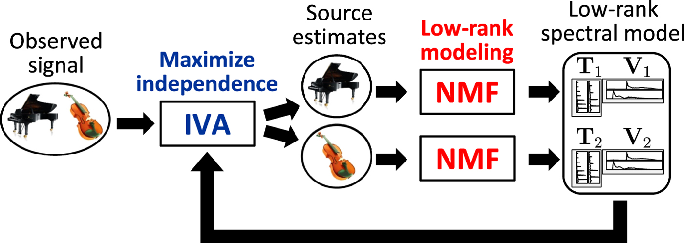
Fig. 7. ILRMA: unified method of IVA and NMF.
2) Restricting MNMF
The second way is to restrict MNMF in the following manner for computational efficiency. Let the spatial property matrix  ${\ssf H}_{in}$ be restricted to rank-1 ${\ssf H}_{in}={\bf h}_{in}{\bf h}_{in}^{\ssf H}$ with ${\bf h}_{in} = [h_{i1n},\ldots ,h_{iMn}]^{\ssf T}$. Then, the MNMF model (26) can be simplified as
 $$\hat{\ssf X}_{ij} = {\bf H}_i{\bf D}_{ij}{\bf H}_i^{\ssf H}$$
with Hi = [hi1, …, hiN] and an N × N diagonal matrix Dij whose nth diagonal element is
 $$\hat{y}_{ij,n} = \sum_{k=1}^K z_{kn}t_{ik}v_{kj}.$$
We further restrict the mixing system to be determined, i.e., N=M, enabling us to convert the mixing matrix Hi to the separation matrix Wi by  ${\bf H}_i = {\bf W}_i^{-1}$. Substituting (33) into (27), we have
 $$\eqalign{{\cal C}({\cal W},{\bf T},{\bf V},{\bf Z}) &=\sum_{i=1}^I\sum_{j=1}^J\sum_{n=1}^N\left[ \displaystyle{\vert y_{ij,n}\vert ^2 \over \hat{y}_{ij,n}} + \log\hat{y}_{ij,n} \right]\cr &\quad -2J\sum_{i=1}^I\log\vert {\rm det}\,{\bf W}_i\vert.}$$
3) Difference between two models
The two ILRMA objective functions (32) and (35) are different in the models (31) and (34) of the source estimates. In (31), the NMF bases are not shared among the source estimates n through the optimization process. In (34), the NMF bases are shared at the beginning of the optimization in accordance with randomly generated cluster-assignment variables 0 ≤ z kn ≤ 1, and assigned dynamically to the source estimates by optimizing the variable z kn.
How to optimize the objective functions (32) and (35) will be explained in the next section.
III. OPTIMIZATION
The objective functions (8), (13), (19), (25), (27), (32), and (35) can be optimized in various ways. Regarding ICA (8), for instance, gradient descent [Reference Bell and Sejnowski23], natural gradient [Reference Amari, Cichocki, Yang, Touretzky, Mozer and Hasselmo24], FastICA [Reference Bingham and Hyvärinen27,Reference Hyvärinen90], and auxiliary function-based optimization (AuxICA) [Reference Ono and Miyabe29], to name a few, have been proposed as optimization methods. This paper focuses on an auxiliary function approach because all the above objective functions can efficiently be optimized by updates derived from this approach.
A) Auxiliary function approach
This subsection explains the general framework of the approach known as the majorization-minimization algorithm [Reference Lange, Hunter and Yang61–Reference Hunter and Lange63]. Let θ be a set of objective variables, e.g., θ = {T, V} in the case of NMF (19). For an objective function  ${\cal C} (\theta )$, an auxiliary function ${\cal C} ^+(\theta, \tilde{\theta})$ with a set of auxiliary variables $\tilde{\theta}$ satisfies the following two conditions.
• The auxiliary function is greater or equal to the objective function
(36) $$ {\cal C}^+(\theta,\tilde{\theta}) \geq {\cal C}(\theta).$$
• When minimized with respect to the auxiliary variables, both functions become the same,
(37)$$ {\rm min}_{\tilde{\theta}}\,{\cal C}^+(\theta,\tilde{\theta}) = {\cal C}(\theta).$$


With these conditions, one can indirectly minimize the objective function  ${\cal C} (\theta)$ by minimizing the auxiliary function ${\cal C} ^+(\theta ,\tilde{\theta})$ through the iteration of the following updates:
(i) the update of auxiliary variables
(38)$$ \tilde{\theta}^{(\ell)} \leftarrow {\rm argmin}_{\tilde{\theta}}\, {\cal C}^+(\theta^{(\ell-1)},\tilde{\theta}) ,$$(ii) the update of objective variables
(39)$$ \theta^{(\ell)} \leftarrow {\rm argmin}_{\theta}\, {\cal C}^+(\theta,\tilde{\theta}^{(\ell)}),$$


as illustrated in Fig. 8. The superscript  $\cdot ^{(\ell )}$ indicates that the update is in the ℓth iteration, starting from the initial sets θ(0) and $\tilde{\theta}^{(0)}$ of variables (randomly initialized in most cases).
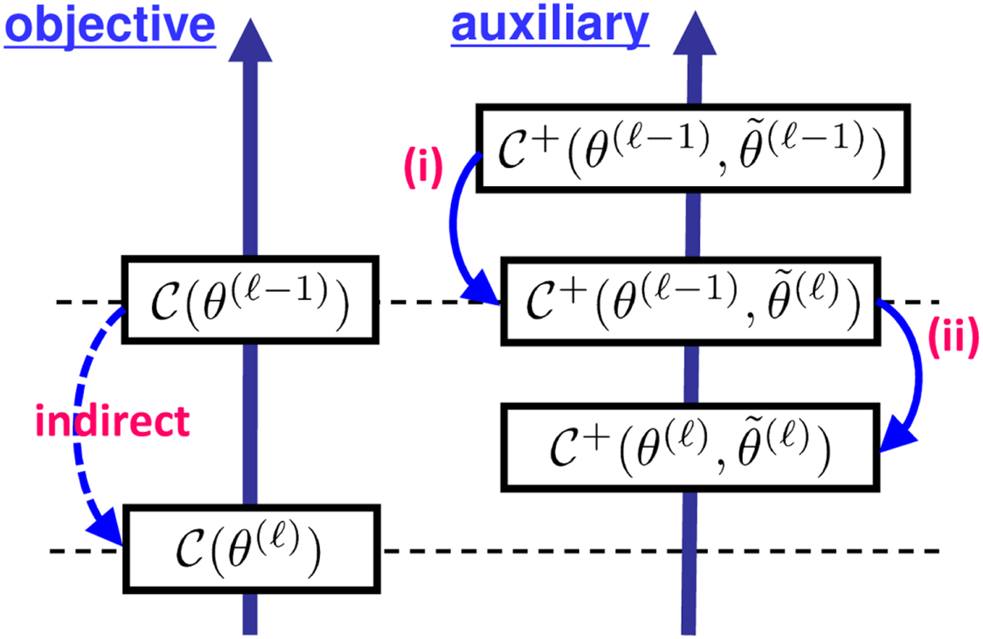
Fig. 8. Majorization-minimization: minimizing the auxiliary function indirectly minimizes the objective function.
A typical situation in which this approach is taken is that the objective function is complicated and not easy to directly minimize but an auxiliary function can be defined in a way that it is easy to minimize.
In the next three subsections, we explain how to minimize the objective functions introduced in Section II. The order is NMF/MNMF, IVA/ICA, and ILRMA, which is different from that of Section II. The reason why the NMF/MNMF case comes first is that the derivation is simpler than the IVA/ICA case and directly by the auxiliary function approach.
B) NMF and MNMF
1) NMF
For the objective function (19) with  $\hat{x}_{ij}$ defined in (15), we employ the auxiliary function
 $$\eqalign{&{\cal C}^+({\bf T},{\bf V},{\cal R},{\bf Q})\cr &\quad = \sum_{i=1}^I\sum_{j=1}^J \left[ \sum_{k=1}^K \displaystyle{r_{ij,k}^2\vert x_{ij}\vert ^2 \over t_{ik}v_{kj}} + \displaystyle{\hat{x}_{ij} \over q_{ij}} + \log q_{ij} -1 \right],}$$
with auxiliary variables  ${\cal R}$, $[{\cal R}]_{ij,k} = r_{ij,k}$, and Q, [Q]ij = q ij, that satisfy r ij,k ≥ 0, $\sum _{k=1}^K r_{ij,k} = 1$ and q ij > 0. The auxiliary function ${\cal C} ^+$ satisfies conditions (36) and (37) because the following two equations hold. The first one,
 $$\displaystyle{1 \over \hat{x}_{ij}} = \displaystyle{1 \over \sum_{k=1}^K t_{ik}v_{kj}} \leq \sum_{k=1}^K \displaystyle{r_{ij,k}^2 \over t_{ik}v_{kj}},$$
originates from the fact that a reciprocal function is convex and therefore satisfies Jensen's inequality. The equality holds when  $r_{ij,k} = ({t_{ik}v_{kj}})/({\hat{x}_{ij}})$. The second one,
 $$ \log \hat{x}_{ij} \leq \log q_{ij} + \displaystyle{\hat{x}_{ij}-q_{ij} \over q_{ij}} ,$$
is derived by the Taylor expansion of the logarithmic function. The equality holds when  $q_{ij} = \hat{x}_{ij}$.
The update (38) of the auxiliary variables is directly derived from the above equality conditions,
 $$ r_{ij,k} \leftarrow \displaystyle{t_{ik}v_{kj} \over \hat{x}_{ij}}, \ {}^{\forall}i,j,k \quad {\rm and} \quad q_{ij} \leftarrow \hat{x}_{ij} , {}^{\forall}i,j .$$
The update (39) of the objective variables is derived by letting the partial derivatives of  ${\cal C} ^+$ with respect to the variables T and V be zero,
 $$\eqalign{& t_{ik}^2 \leftarrow \displaystyle{\sum_{j=1}^J({r_{ij,k}^2\vert x_{ij}\vert ^2})/({v_{kj}}) \over \sum_{j=1}^J({v_{kj}})/({q_{ij}}) } \quad {\rm and}\cr & v_{kj}^2 \leftarrow \displaystyle{\sum_{i=1}^I({r_{ij,k}^2\vert x_{ij}\vert ^2})/({t_{ik}}) \over \sum_{i=1}^I({t_{ik}})/({q_{ij}})}.}$$
Substituting (43) into (44) and simplifying the resulting expressions, we have well-known multiplicative update rules
 $$\eqalign{&t_{ik} \leftarrow t_{ik} \sqrt{\displaystyle{\sum_{j=1}^J(({v_{kj}})/({\hat{x}_{ij}}))({\vert x_{ij}\vert ^2})/({\hat{x}_{ij}}) \over \sum_{j=1}^J({v_{kj}})/({\hat{x}_{ij}})} } \cr &v_{kj} \leftarrow v_{kj}\sqrt{ \displaystyle{\sum_{i=1}^I(({t_{ik}})/({\hat{x}_{ij}}))({\vert x_{ij}\vert ^2})/({\hat{x}_{ij}}) \over \sum_{i=1}^I({t_{ik}})/({\hat{x}_{ij}})} },}$$
for minimizing the IS-NMF objective function (19).
2) MNMF
The derivation of the NMF update rules can be extended to MNMF. Let us first introduce auxiliary variables  ${\ssf R}_{ij,k}$ and ${\ssf Q}_{ij}$ of M × M Hermitian positive semidefinite matrices as extensions of r ij,k and q ij, respectively. Then, for the MNMF objective function (25), let us employ the auxiliary function
 $$\eqalign{& {\cal C}^+({\bf T},{\bf V},\underline{\bf H}, \underline{\cal R},\underline{\bf Q})\cr &\quad = \sum_{i=1}^I\sum_{j=1}^J \sum_{k=1}^K \displaystyle{{\bf x}_{ij}^{\ssf H}{\ssf R}_{ij,k}{\ssf H}_{ik}^{-1}{\ssf R}_{ij,k} {\bf x}_{ij} \over t_{ik}v_{kj}} \cr &\qquad + \sum_{i=1}^I\sum_{j=1}^J \left[ {\rm tr}(\hat{\ssf X}_{ij}{\ssf Q}_{ij}^{-1}) + \log{\rm det}\,{\ssf Q}_{ij} -M \right],}$$
with auxiliary variables  $\underline{\cal R}$, $[\underline{\cal R}]_{ij,k} = {\ssf R}_{ij,k}$, and $\underline{\bf Q}$, $[\underline{\bf Q}]_{ij}={\ssf Q}_{ij}$, that satisfy $\sum _{k=1}^K {\ssf R}_{ij,k} = {\ssf I}$ with ${\ssf I}$ being the identity matrix of size M. The auxiliary function ${\cal C} ^+$ satisfies the conditions (36) and (37) because the following two equations hold. The first one,
 $${\rm tr} \left[\left(\sum_{k=1}^K{\ssf H}_{ik}t_{ik}v_{kj}\right)^{-1} \right] \leq \sum_{k=1}^K \displaystyle{{\rm tr}({\ssf R}_{ij,k}{\ssf H}_{ik}^{-1}{\ssf R}_{ij,k}) \over t_{ik}v_{kj}} ,$$
is a matrix extension of (41). The equality holds when  ${\ssf R}_{ij,k} = t_{ik}v_{kj}{\ssf H}_{ik}\hat{\ssf X}_{ij}^{-1}$. The second one [Reference Yoshii, Tomioka, Mochihashi and Goto66],
 $$ \log{\rm det}\hat{\ssf X}_{ij} \leq \log{\rm det}\,{\ssf Q}_{ij} + {\rm tr}( \hat{\ssf X}_{ij}{\ssf Q}_{ij}^{-1}) -M ,$$
is a matrix extension of (42). The equality holds when  ${\ssf Q}_{ij} = \hat{\ssf X}_{ij}$.
The update (38) of the auxiliary variables is directly derived from the above equality conditions,
 $$ {\ssf R}_{ij,k} \leftarrow t_{ik}v_{kj}{\ssf H}_{ik}\hat{\ssf X}_{ij}^{-1} , {}^\forall i,j,k \quad {\rm and} \quad {\ssf Q}_{ij} \leftarrow \hat{\ssf X}_{ij}, {}^{\forall}i,j.$$
The update (39) of the objective variables is derived by letting the partial derivatives of  ${\cal C} ^+$ with respect to the variables T, V, and $\underline{\bf H}$ be zero,
 $$\eqalign{&t_{ik}^2 \leftarrow \displaystyle{\sum_{j=1}^J ({1}/{v_{kj}}) {\bf x}_{ij}^{\ssf H}{\ssf R}_{ij,k}{\ssf H}_{ik}^{-1}{\ssf R}_{ij,k}{\bf x}_{ij} \over \sum_{j=1}^J v_{kj} {\rm tr}({\ssf Q}_{ij}^{-1}{\ssf H}_{ik}) } \cr &v_{ik}^2 \leftarrow \displaystyle{\sum_{i=1}^I ({1}/{t_{ik}}) {\bf x}_{ij}^{\ssf H}{\ssf R}_{ij,k}{\ssf H}_{ik}^{-1}{\ssf R}_{ij,k}{\bf x}_{ij} \over \sum_{i=1}^I t_{ik} {\rm tr}({\ssf Q}_{ij}^{-1}{\ssf H}_{ik}) } \cr {\ssf H}_{ik} &\left( t_{ik}\sum_{j=1}^J{\ssf Q}_{ij}^{-1}v_{kj}\right) {\ssf H}_{ik} = \sum_{j=1}^J \displaystyle{{\ssf R}_{ij,k}{\ssf X}_{ij}{\ssf R}_{ij,k} \over t_{ik}v_{kj}}.}$$
Substituting (50) into (51) and simplifying the resulting expressions, we have the following multiplicative update rules for minimizing the MNMF objective function (25):
 $$ \eqalign{& t_{ik} \leftarrow t_{ik}\sqrt{\displaystyle{\sum_{j=1}^J v_{kj} {\bf x}_{ij}^{\ssf H}\hat{\ssf X}_{ij}^{-1}{\ssf H}_{ik}\hat{\ssf X}_{ij}^{-1}{\bf x}_{ij} \over \sum_{j=1}^J v_{kj} {\rm tr}(\hat{\ssf X}_{ij}^{-1}{\ssf H}_{ik})}}\cr & v_{kj} \leftarrow v_{kj}\sqrt{\displaystyle{\sum_{i=1}^I t_{ik} {\bf x}_{ij}^{\ssf H}\hat{\ssf X}_{ij}^{-1}{\ssf H}_{ik}\hat{\ssf X}_{ij}^{-1}{\bf x}_{ij} \over \sum_{i=1}^I t_{ik} {\rm tr}(\hat{\ssf X}_{ij}^{-1}{\ssf H}_{ik})} }\cr & {\ssf H}_{ik} \leftarrow {\ssf A}^{-1}\#({\ssf H}_{ik}{\ssf B}{\ssf H}_{ik}),}$$
where # calculates the geometric mean [Reference Yoshii, Kitamura, Bando, Nakamura and Kawahara91] of two positive semidefinite matrices as
 $$ {\ssf X}\#{\ssf Y} = {\ssf X}({\ssf X}^{-1}{\ssf Y})^{1/2}$$
and  ${\ssf A}=\sum_{j=1}^J v_{kj}\hat{\ssf X}_{ij}^{-1}$ and ${\ssf B}=\sum _{j=1}^J v_{kj}\hat{\ssf X}_{ij}^{-1}{\ssf X}_{ij}\hat{\ssf X}_{ij}^{-1}$.
So far, we have explained the optimization of the objective function (25). The other objective function, (27) with (26), can be optimized similarly [Reference Sawada, Kameoka, Araki and Ueda49].
C) IVA and ICA
We next explain how to minimize the IVA objective function (13). The ICA case (8) can simply be derived by letting I=1 in the IVA case.
1) Auxiliary function for contrast function
Since the contrast function G(yj,n) = −log p(yj,n) is generally a complicated part to be minimized, we first discuss an auxiliary function for a contrast function. The contrast function with the density (14) is given as
 $$G({\bf y}_{j,n})=\displaystyle{1 \over \beta}\sqrt{\vert \vert {\bf y}_{j,n}\vert \vert _2^2+\alpha}$$
with
 $$\vert \vert {\bf y}_{j,n}\vert \vert _2 = \sqrt{\sum_{i=1}^I \vert y_{ij,n}\vert ^2}$$
being the L2 norm. It is common that a contrast function depends only on the L2 norm. If there is a real-valued function G R(r j,n) that satisfies G R(||yj,n||2) = G(yj,n) and G′R(r j,n)/r j,n is monotonically decreasing in r j,n ≥ 0, we have an auxiliary function,
 $$ G^+({\bf y}_{j,n}, r_{j,n}) = \displaystyle{G'_R(r_{j,n}) \over 2r_{j,n}} \vert \vert {\bf y}_{j,n}\vert \vert _2^2 + F(r_{j,n}),$$
that satisfies [Reference Ono43] the two conditions (36) and (37). The term F(r j,n) does not depend on the objective variable yj,n. The equality holds when r j,n = ||yj,n||2. For the density function (14), the coefficient ((G′R(r j,n))/(2r j,n)) is given as
 $$\displaystyle{1 \over 2\beta\sqrt{r_{j,n}^2+\alpha}}.$$
2) Auxiliary function for objective function
Now, we introduce an auxiliary function for the IVA objective function (13) by simply replacing G(yj,n) with G +(yj,n, r j,n),
 $$ {\cal C}^+({\cal W}, {\bf R}) = \sum_{j=1}^J \sum_{n=1}^N G^+({\bf y}_{j,n}, r_{j,n}) -2J\sum_{i=1}^I \log\vert {\rm det}\,{\bf W}_i\vert,$$
with auxiliary variables R, [R]j,n = r j,n. The equality  ${\cal C} ^+({\cal W}, {\bf R}) = {\cal C} ({\cal W})$ is satisfied when r j,n = ||yj,n||2 for all j = 1, …, J and n = 1, …, N. This corresponds to the update (38) of the auxiliary variables.
For the minimization of  ${\cal C} ^+$ with respect to the set ${\cal W}=\{{\bf W}_i\}_{i=1}^I$ of separation matrices
 $$ {\bf W}_i = \left[\matrix{{\bf w}_{i,1}^{\ssf H} \cr \vdots \cr {\bf w}_{i,N}^{\ssf H}} \right],$$
let the auxiliary function  ${\cal C} ^+$ be rewritten as follows by omitting the terms F(r j,n) that do not depend on ${\cal W}$:
 $$ J\sum_{i=1}^I \left[\sum_{n=1}^N {\bf w}_{i,n}^{\ssf H}{\bf U}_{i,n}{\bf w}_{i,n} -2 \log\vert {\rm det}\,{\bf W}_i\vert \right]$$
 $${\bf U}_{i,n} = \displaystyle{1 \over J}\sum_{j=1}^J \displaystyle{G'_R(r_{j,n}) \over 2r_{j,n}} {\bf x}_{ij}{\bf x}_{ij}^{\ssf H}.$$
 Note that  $\vert \vert {\bf y}_{j,n}\vert \vert _2^2=\sum _{i=1}^I y_{ij,n} y_{ij,n}^{\ast}$ and $y_{ij,n}={\bf w}_{i,n}^{\ssf H}{\bf x}_{ij}$ from (4) are used in the rewriting. Letting the gradient $({\partial {\cal C} ^+})/({\partial {\bf w}_{i,n}^{\ast}})$ of (55), equivalently the gradient of (57), with respect to wi,n* be zero, we have N simultaneous equations [Reference Ono43],
 $$ {\bf w}_{i,m}^{\ssf H} {\bf U}_{i,n} {\bf w}_{i,n} = \delta_{mn}, \quad m=1,\ldots,N,$$
where δmn is the Kronecker delta. Considering all N rows of the separation matrix (56), we then have N × N simultaneous equations, i.e., (59) for n = 1, …, N. This problem has been formulated as the hybrid exact-approximate diagonalization (HEAD) [Reference Yeredor92] for Ui,1, …, Ui,N. Solving HEAD problems to update Wi for i = 1, …, I constitutes the update (39) of the objective variables.
3) Solving the HEAD problem
An efficient way [Reference Ono43] to solve the HEAD problem for a separation matrix Wi is to calculate
 $$ {\bf w}_{i,n} \leftarrow ({\bf W}_i {\bf U}_{i,n})^{-1} {\bf e}_n,$$
for each n, where en is the vector whose nth element is one and the other elements are zero, and update it as
 $$ {\bf w}_{i,n} \leftarrow \displaystyle{{\bf w}_{i,n} \over \sqrt{{\bf w}_{i,n}^{\ssf H}{\bf U}_{i,n}{\bf w}_{i,n}}},$$
to accommodate the HEAD constraint  ${\bf w}_{i,n}^{\ssf H}{\bf U}_{i,n}{\bf w}_{i,n}=1$.
4) Whole AuxIVA algorithm
Algorithm 1 summarizes the procedures discussed so far in this subsection. To be concrete, the algorithm description is specific to the case of the super-Gaussian density (14).

D) ILRMA
The ILRMA objective function (32) can be minimized by alternating NMF updates similar to (45) and the HEAD problem solver (as the IVA part), as illustrated in Fig. 7.
Let us first consider the NMF updates of  $\{{\bf T}_n\}_{n=1}^N$ and $\{{\bf V}_n\}_{n=1}^N$ by focusing on the first term of (32). Note that for each n, the objective function is the same as (19) if |y ij,n|2 and $\hat{y}_{ij,n}$ are replaced with |x ij|2 and $\hat{x}_{ij}$, respectively. We thus have the following updates for n = 1, …, N:
 $$\matrix{t_{ik,n} \leftarrow t_{ik,n}\sqrt{ \displaystyle{\sum_{j=1}^J(({v_{kj,n}})/({\hat{y}_{ij,n}}))(({\vert y_{ij,n}\vert ^2}/( {\hat{y}_{ij}})) \over \sum_{j=1}^J({v_{kj,n}})/({\hat{y}_{ij,n}})} } \cr v_{kj,n} \leftarrow v_{kj,n}\sqrt{ \displaystyle{\sum_{i=1}^I(({t_{ik,n}})/({\hat{y}_{ij,n}}))(({\vert y_{ij,n}\vert ^2})/( {\hat{y}_{ij,n}})) \over \sum_{i=1}^I({t_{ik,n}})/({\hat{y}_{ij,n}})}}.}$$
 Next we consider the update of  ${\cal W}$ as the IVA part. For the objective function (32), let us omit the $\log \hat{y}_{ij,n}$ terms that do not depend on ${\cal W}$,
 $$ \sum_{n=1}^N\sum_{i=1}^I\sum_{j=1}^J \displaystyle{\vert y_{ij,n}\vert ^2 \over \hat{y}_{ij,n}} -2J\sum_{i=1}^I\log \vert {\rm det}\,{\bf W}_i\vert,$$
and then rewrite it in a similar way to (56),
 $$J\sum_{i=1}^I\left[\sum_{n=1}^N {\bf w}_{i,n}^{\ssf H}{\bf U}_{i,n}{\bf w}_{i,n} -2\log \vert {\rm det}\,{\bf W}_i\vert \right],$$
 $${\bf U}_{i,n} = \displaystyle{1 \over J}\sum_{j=1}^J \displaystyle{1 \over \hat{y}_{ij,n}} {\bf x}_{ij}{\bf x}_{ij}^{\ssf H}.$$
Since (63) has the same form as (56), the optimization reduces to solving the HEAD problem for the weighted covariance matrices (64).
Note that no auxiliary function is used to derive (63), unlike in the derivation of (56). A very similar objective function to (62) is derived for the IVA objective function (13) if we assume a Gaussian with time-varying variance  $\sigma _{j,n}^2$ [Reference Ono44],
 $$ p({\bf y}_{j,n}) \propto \displaystyle{1 \over \sigma_{j,n}^2} \exp\left(-\displaystyle{\sum_{i=1}^I \vert y_{ij,n}\vert ^2 \over \sigma_{j,n}^2}\right).$$
The difference between the objective functions is in  $\hat{y}_{ij,n}$ and $\sigma _{j,n}^2$, and this difference exactly corresponds to the difference between ILRMA and IVA (see Fig. 4 in [Reference Kitamura, Ono, Sawada, Kameoka and Saruwatari56], where ILRMA was called determined rank-1 MNMF).
So far, we have explained the optimization of the objective function (32). The other objective function, (35) with (34), can be optimized similarly [Reference Kitamura, Ono, Sawada, Kameoka and Saruwatari56].
IV. EXPERIMENT
This section shows experimental results of the discussed methods for a simple two-source two-microphone situation. Since this paper is a review paper, detailed experimental results under a variety of conditions are not shown here. Such experimental results can be found in the original papers, e.g., [Reference Sawada, Kameoka, Araki and Ueda49,Reference Kitamura, Ono, Sawada, Kameoka and Saruwatari56]. The purpose of this section is to illustrate the characteristics of the reviewed five methods (ICA, IVA, ILRMA, NMF, MNMF).
In the experiment, we measured impulse responses from two loudspeakers to two microphones in a room whose reverberation time was RT60 = 200 ms. Then, a music source and a speech source were convolved (their source images at the first microphone are shown at the left most of Fig. 9) and mixed for 8-second microphone observations. The sampling frequency was 8 kHz. The frame width and shift of the STFT were 256 ms and 64 ms, respectively. For the density functions of ICA (9) and IVA (14), we set the parameters as α = β = 0.01. The number of update iterations was 50 for ICA, IVA, ILRMA, and NMF to attain sufficient separations. However, for MNMF, 50 was insufficient and we iterated the updates 200 times to obtain sufficient separations.
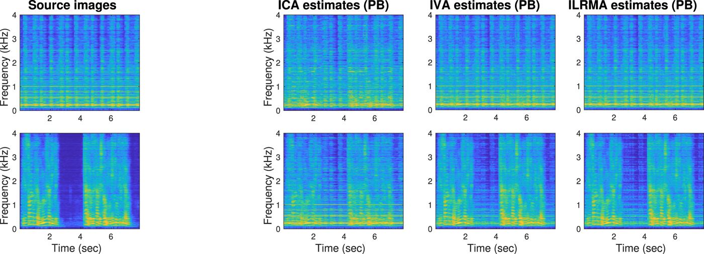
Fig. 9. Source images (left-most column) and source estimates by ICA, IVA, and ILRMA (three columns on the right) whose scales were adjusted by projection back (PB). The first and second rows correspond to music and speech sources, respectively. The plots are spectrograms colored in log scale with large values being yellow. The ICA estimates were not well separated in a full-band sense (SDRs = 6.27 dB, 1.38 dB). The IVA estimations were well separated (SDRs = 13.52 dB, 8.79 dB). The ILRMA estimates were even better separated (SDRs = 16.78 dB, 12.33 dB). Detailed investigations are shown in Fig. 10.
The three plots in the right-hand side of Fig. 9 show the separation results obtained by ICA, IVA, and ILRMA. These are the spectrograms after scaling ambiguities were adjusted to the source images shown in the leftmost by the projection back (PB) approach [Reference Cardoso93–Reference Mori97], specifically by the procedure described in [Reference Sawada, Araki and Makino98]. Signal-to-distortion ratios (SDRs) [Reference Vincent99] are reported in the captions to show how well the results were separated. To investigate the characteristics of these methods, Fig. 10 shows the source estimates without PB and related auxiliary variables. Specifically, in this example, the speech source had a pause at around from 3 to 4 seconds. Some of the IVA variables R and ILRMA variables V shown in the bottom row successfully extracted the pause and contributed to the separation.
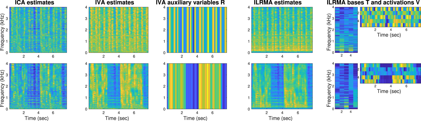
Fig. 10. (Continued from Fig. 9) Source estimates and auxiliary variables of ICA, IVA, and ILRMA. The source estimates y ij,n were not scale-adjusted, and had direct links to the auxiliary variables. The ICA estimates were not well separated because there was no communication channel among frequency bins (auxiliary variables used in the other two methods) and the permutation problem was not solved. The IVA estimates were well separated. The IVA auxiliary variables R, [R]j,n = r j,n, represented the activities of source estimates and helped to solve the permutation problem. The ILRMA estimates were even better separated. The ILRMA bases T and activations V, [Tn]ik = t ik,n, [Vn]kj = v kj,n, modeled the source estimates with low-rank matrices, which were richer representations than the IVA auxiliary variables R.
Figure 11 shows how NMF and MNMF modeled and separated the two-channel mixtures. NMF extracted 10 bases for each channel. However, there was no link between the bases and sources. Therefore, separation to two sources was not attained in the NMF case. In the MNMF case, 10 NMF bases were extracted for the multichannel mixtures, and clustered and separated into two sources.
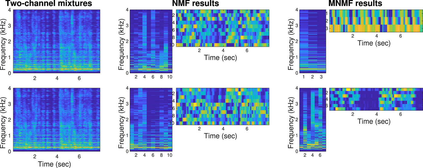
Fig. 11. Experimental mixtures and variables (log scale, large values in yellow) of NMF and MNMF. The Two-channel mixtures look very similar in a power spectrum sense. However, the phases (not shown) are considerably different to achieve effective multichannel separation. The NMF results were obtained corresponding to each mixture. No multichannel information was exploited, and thus the two sources were not separated. In the MNMF results, 10 NMF bases were clustered into two classes according to the multichannel information  ${\ssf H}_{in}$ in the model (26). The off-diagonal elements $[{\ssf H}_{in}]_{mm'}, m\ne m'$, expressed the phase differences between the microphones as spatial cues, and the two sources were well separated (SDRs = 14.96 dB, 10.31 dB).
V. CONCLUSION
Five methods for BSS of audio signals have been explained. ICA and IVA resort to the independence and super-Gaussianity of sources. NMF and MNMF model spectrograms with low-rank structures. ILRMA integrates these two different lines of methods and exploits the independence and the low-rankness of sources. All the objective functions regarding these methods can be optimized by auxiliary function approaches. This review paper has explained these facts in a structured and concise manner, and hopefully will contribute to the development of further methods for BSS.
Hiroshi Sawada received the B.E., M.E., and Ph.D. degrees in information science from Kyoto University, in 1991, 1993, and 2001, respectively. He joined NTT Corporation in 1993. He is now a senior distinguished researcher and an executive manager at the NTT Communication Science Laboratories. His research interests include statistical signal processing, audio source separation, array signal processing, latent variable models, and computer architecture. From 2006 to 2009, he served as an associate editor of the IEEE Transactions on Audio, Speech & Language Processing. He is an associate member of the Audio and Acoustic Signal Processing Technical Committee of the IEEE SP Society. He received the Best Paper Award of the IEEE Circuit and System Society in 2000, the SPIE ICA Unsupervised Learning Pioneer Award in 2013, the IEEE Signal Processing Society 2014 Best Paper Award. He is an IEEE Fellow, an IEICE Fellow, and a member of the ASJ.
Nobutaka Ono received the B.E., M.S., and Ph.D. degrees from the University of Tokyo, Japan, in 1996, 1998, 2001, respectively. He became a research associate in 2001 and a lecturer in 2005 in the University of Tokyo. He moved to the National Institute of Informatics in 2011 as an associate professor, and moved to Tokyo Metropolitan University in 2017 as a full professor. His research interests include acoustic signal processing, machine learning, and optimization algorithms for them. He was a chair of Signal Separation Evaluation Campaign evaluation committee in 2013 and 2015, and an Associate Editor of the IEEE Transactions on Audio, Speech and Language Processing during 2012 to 2015. He is a senior member of the IEEE Signal Processing Society and a member of IEEE Audio and Acoustic Signal Processing Technical Committee from 2014. He received the unsupervised learning ICA pioneer award from SPIE.DSS in 2015.
Hirokazu Kameoka received B.E., M.S., and Ph.D. degrees all from the University of Tokyo, Japan, in 2002, 2004, and 2007, respectively. He is currently a Distinguished Researcher and a Senior Research Scientist at NTT Communication Science Laboratories, Nippon Telegraph and Telephone Corporation and an Adjunct Associate Professor at the National Institute of Informatics. From 2011 to 2016, he was an Adjunct Associate Professor at the University of Tokyo. His research interests include audio, speech, and music signal processing and machine learning. He has been an associate editor of the IEEE/ACM Transactions on Audio, Speech, and Language Processing since 2015, a Member of IEEE Audio and Acoustic Signal Processing Technical Committee since 2017, and a Member of IEEE Machine Learning for Signal Processing Technical Committee since 2019. He received 17 awards, including the IEEE Signal Processing Society 2008 SPS Young Author Best Paper Award.
Daichi Kitamura received the M.E. and Ph.D. degrees from Nara Institute of Science and Technology and SOKENDAI (The Graduate University for Advanced Studies), respectively. He joined The University of Tokyo in 2017 as a Research Associate, and he moved to National Institute of Technology, Kagawa Collage as an Assistant Professor in 2018. His research interests include audio source separation, array signal processing, and statistical signal processing. He received Awaya Prize Young Researcher Award from The Acoustical Society of Japan (ASJ) in 2015, Ikushi Prize from Japan Society for the Promotion of Science in 2017, Best Paper Award from IEEE Signal Processing Society Japan in 2017, and Itakura Prize Innovative Young Researcher Award from ASJ in 2018. He is a member of IEEE and ASJ.
Hiroshi Saruwatari Hiroshi Saruwatari received the B.E., M.E., and Ph.D. degrees from Nagoya University, Japan, in 1991, 1993, and 2000, respectively. He joined SECOM IS Laboratory, Japan, in 1993, and Nara Institute of Science and Technology, Japan, in 2000. From 2014, he is currently a Professor of The University of Tokyo, Japan. His research interests include audio and speech signal processing, blind source separation, etc. He received paper awards from IEICE in 2001 and 2006, from TAF in 2004, 2009, 2012, and 2018, from IEEE-IROS2005 in 2006, and from APSIPA in 2013 and 2018. He received DOCOMO Mobile Science Award in 2011, Ichimura Award in 2013, The Commendation for Science and Technology by the Minister of Education in 2015, Achievement Award from IEICE in 2017, and Hoko-Award in 2018. He has been professionally involved in various volunteer works for IEEE, EURASIP, IEICE, and ASJ. He is an APSIPA Distinguished Lecturer from 2018.


 Open access