Laplacian networks: bounding indicator function smoothness for neural networks robustness

Carlos Lassance; Vincent Gripon; Antonio Ortega

doi:10.1017/ATSIP.2021.2

Laplacian networks: bounding indicator function smoothness for neural networks robustness

Published online by Cambridge University Press: 05 February 2021

Carlos Lassance

Vincent Gripon and

Antonio Ortega

Show author details

Carlos Lassance*: Affiliation:
Département Électronique, IMT Atlantique, 655 Avenue du Technopôle, Brest29280, France
Vincent Gripon: Affiliation:
Département Électronique, IMT Atlantique, 655 Avenue du Technopôle, Brest29280, France
Antonio Ortega: Affiliation:
Department of Electrical and Computer Engineering, Signal and Image Processing Institute, University of Southern California, 3740 McClintock Ave., EEB 436, Los Angeles, CA90089-2564, USA
*: Corresponding author: Carlos Lassance Email: cadurosar@gmail.com

Article contents

Abstract
INTRODUCTION
METHODOLOGY
EXPERIMENTS
CONCLUSION
Footnotes
References

Abstract

For the past few years, deep learning (DL) robustness (i.e. the ability to maintain the same decision when inputs are subject to perturbations) has become a question of paramount importance, in particular in settings where misclassification can have dramatic consequences. To address this question, authors have proposed different approaches, such as adding regularizers or training using noisy examples. In this paper we introduce a regularizer based on the Laplacian of similarity graphs obtained from the representation of training data at each layer of the DL architecture. This regularizer penalizes large changes (across consecutive layers in the architecture) in the distance between examples of different classes, and as such enforces smooth variations of the class boundaries. We provide theoretical justification for this regularizer and demonstrate its effectiveness to improve robustness on classical supervised learning vision datasets for various types of perturbations. We also show it can be combined with existing methods to increase overall robustness.

Keywords

Machine learning Robustness Graph signal processing Laplacian Adversarial attacks

Type: Original Paper
Information: APSIPA Transactions on Signal and Information Processing , Volume 10 , 2021 , e2

DOI: https://doi.org/10.1017/ATSIP.2021.2 [Opens in a new window]
Creative Commons: This is an Open Access article, distributed under the terms of the Creative Commons Attribution licence (http://creativecommons.org/licenses/by/4.0/), which permits unrestricted re-use, distribution, and reproduction in any medium, provided the original work is properly cited.
Copyright: Copyright © The Author(s), 2021. Published by Cambridge University Press.

I. INTRODUCTION

Deep learning (DL) networks provide state-of-the-art performance for many machine-learning tasks [Reference He, Zhang, Ren and Sun1, Reference Wu, Schuster, Chen, Le, Norouzi, Macherey, Krikun, Cao, Gao and Macherey2]. Their ability to achieve good generalization is often explained by the fact they use very few priors about data [Reference LeCun, Bengio and Hinton3]. On the other hand, their strong dependency on data may lead to selection of biased features of the training dataset, resulting in a lack of robustness in classification performance. Here robustness refers to the ability of a classifier to infer correctly even when the inputs (or the parameters of the classifier) are subject to perturbations. These perturbations can be due to general factors – such as noise, quantization of inputs or parameters, and adversarial attacks – as well as application specific ones – such as the use of a different camera lens, brightness exposure, or weather, in an imaging task.

An often studied case is that of adversarial attacks, where very small (imperceptible) changes on the input of a trained DL network have been shown to result in its misclassification [Reference Szegedy4, Reference Goodfellow, Shlens and Szegedy5], thus providing evidence that DL networks may not be as robust to perturbations as the test accuracy would lead one to believe. In practice, in many applications it is unlikely that there would be adversaries, and in particular adversaries having access to the network parameters that are required to build these perturbations. This is why recent study advocates focusing on more realistic robustness [Reference Gilmer, Adams, Goodfellow, Andersen and Dahl6], i.e. considering perturbations that are not linked to adversarial (or deliberate) noise [Reference Hendrycks and Dietterich7].

Proposed approaches to improve robustness can be roughly divided into three classes: (i) changes in the inference methods, (ii) introduction of regularizers, and (iii) ad-hoc data augmentation. Inference methods use a procedure for prediction that differs from the one the network has been trained on (i.e. unlike the classic $\arg \max$ classifier), e.g. based on a model ensemble composed of $k$-nearest neighbors classifiers for each layer [Reference Papernot and McDaniel8]. Methods introducing regularizers range from minimizing the squared norm Jacobian [Reference Gu and Rigazio9] to controlling the Lipschitz constant of the network function via regularization [Reference Mallat10, Reference Cisse, Bojanowski, Grave, Dauphin and Usunier11]. Note that bounding the Lipschitz constant of the network as proposed in these studies can be inconsistent with the training objective. We discuss this in further detail in Section II.A. Finally data-augmentation methods revolve around using deformed inputs during the training phase so that the network function generalizes better to the corresponding perturbations [Reference Goodfellow, Shlens and Szegedy5, Reference Pezeshki, Fan, Brakel, Courville and Bengio12–Reference Madry, Makelov, Schmidt, Tsipras and Vladu15]. However, there is no guarantee that training to be robust to some perturbations can universally increase robustness to all types of perturbations, even if using adversarial examples during training.

Our proposed method fits in the second category: we introduce a regularizer that penalizes large deformations of the class boundaries throughout the network architecture, independently of the types of perturbations that we expect to face when the system is deployed. It also enforces a large margin $r$ (i.e. mid-distance between examples of distinct classes) at each layer of the architecture.

To understand the intuition behind our proposed regularizer, first note that networks are typically trained with the objective of yielding zero error for the training set. If error on the training set is (approximately) zero then any two examples with different labels can be separated by the network, even if these examples are close to each other in the original domain. This means that the network function can create significant deformations of the space (small distances in the original domain map to larger distances in the final layers) and explains how an adversarial attack with small changes to the input can lead to class label changes. Our proposed regularizer penalizes big changes at the boundaries between classes. By forcing boundary deformations to evolve smoothly across the architecture, and at the same time by maintaining a large margin, the proposed regularizer therefore favors smooth variations instead, leading to better robustness. We will empirically demonstrate this claim on classical vision datasets.

The proposed regularizer is based on a series of graphs, one for each layer of the DL architecture, where each graph captures the similarity between training examples given their intermediate representation at that layer. Our regularizer favors small changes, from one layer to the next, in the distances between pairs of examples in different classes.Footnote ¹ It achieves so by penalizing large changes in the smoothness (computed using the Laplacian quadratic form) of the class indicator vectors (viewed as “graph signals”). As a result, the margin is kept almost constant across layers, and the deformations of space are controlled at the boundary regions, as illustrated in Fig. 1. This draws heavily from previous studies of some of the authors [Reference Gripon, Ortega and Girault16, Reference Anis, ElGamal, Avestimehr and Ortega17], and uses the robustness definition that was introduced in [Reference Lassance, Gripon, Tang and Ortega18], which was inspired from preliminary versions of this study [Reference Lassance, Gripon and Ortega19]. More generally, combining graphs and DL analysis has sparked a lot of interest recently. For example, Anirudh et al. [Reference Anirudh, Thiagarajan, Sridhar and Bremer20] introduced different quantities related to graph signal processing (GSP) that can be used to extract interpretable results from DL networks, but, unlike our study, does not tackle robustness. Another example is [Reference Svoboda, Masci, Monti, Bronstein and Guibas21] where the authors exploit graph convolutional layers [Reference Bronstein, Bruna, LeCun, Szlam and Vandergheynst22], smoothing the latent representations of the inferred images using images from the training set, in order to increase the robustness of the network. Note that this could be described as a denoising of the inference (test) image, using the training ones. This differs from our study, which focuses on generating a smooth network function.

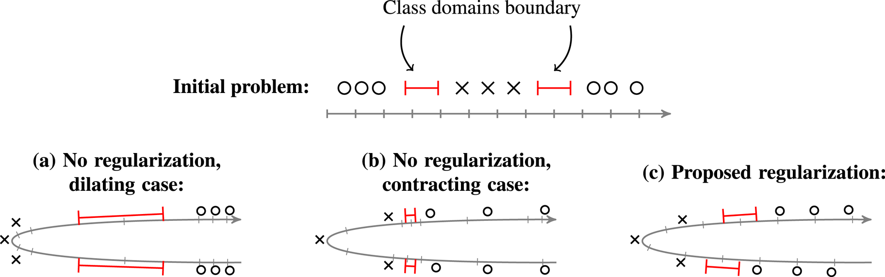
Fig. 1. Illustration of the effect of our proposed regularizer. In this example, the goal is to classify circles and crosses (top). Without use of regularizers (bottom left), the resulting embedding may considerably stretch the boundary regions. Consequently, the risk is to obtain sharp transitions in the network function (that would correspond to a large value of $\alpha$ in equation (2)). Another possible issue would be to push inputs closer to the boundary (bottom center), thus reducing the margin (that would correspond to a small value of $r$ in equation (2)). Forcing small variations of smoothness of label signals (bottom right), we ensure the topology is not dramatically changed in the boundary regions.

In Section III we demonstrate, using readily-available image classification datasets, the robustness of the proposed regularizer to common perturbations studied in the literature: (i) noise [Reference Hendrycks and Dietterich7, Reference Mallat10], for which we show reductions in relative error increase, (ii) adversarial attacks [Reference Szegedy4, Reference Goodfellow, Shlens and Szegedy5], for which the median defense radius [Reference Moosavi Dezfooli, Fawzi and Frossard14] is increased by 50% in comparison with the baseline and by 12% in comparison with another method in the literature [Reference Cisse, Bojanowski, Grave, Dauphin and Usunier11], and (iii) implementation defects, which result in only approximately correct computations [Reference Hubara, Courbariaux, Soudry, El-Yaniv and Bengio23], for which we increase the median accuracy by 48% relative to the baseline and 26% relative to another method in the literature [Reference Cisse, Bojanowski, Grave, Dauphin and Usunier11].

The outline of the paper is as follows. In Section II we introduce the proposed regularizer and our definition of robustness. In Section III we evaluate the performance of our proposed method in various conditions and on vision benchmarks. Section IV summarizes our conclusions.

II. METHODOLOGY

A) Robustness definition

A deep neural network architecture is entirely described by its associated “network function.” This network function $f$ receives an input $\mathbf {x}$ (e.g. a tensor representing the pixel values of an image, normalized so that standard deviation is 1) and outputs a class-wise classification score $f(\mathbf {x})$. Typically this output is a vector with as many coordinates as the number of classes in the problem, where the highest valued coordinate is the decision of the network (i.e. $\arg \max$ classifier). This function is constructed via the composition of multiple intermediate functions $f^\ell$:

(1)\begin{equation} f = f^{L}\circ f^{L-1} \circ \dots \circ f^1, \end{equation}

where each function $f^\ell$ is highly constrained, typically as the concatenation of a parameter-free nonlinear function with a parameterized linear function.

The function $f$ is typically obtained based on a very large number of parameters, which are tuned during the learning phase. During this phase, a loss function is minimized over a set of training examples using a variant of the stochastic gradient descent algorithm. At the end of the training process, each training example is associated through $f$ with a vector whose largest value is the actual class of that example, leading to an accuracy close to 100% on the training set. Importantly, the loss function usually targets a specific margin in the output domain. For example, when using the classical cross-entropy loss, the loss function is minimized when the output of the training examples are the one-hot-bit vectors of their corresponding class [Reference LeCun, Bengio and Hinton3, Reference Goodfellow, Bengio and Courville24], which corresponds to a margin in the output domain of about $\sqrt {2}/2$ for the $\mathcal {L}_2$ norm.

We define network robustness following the ideas in our previous study [Reference Lassance, Gripon, Tang and Ortega18] as:

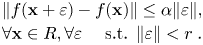
Definition 1 A network function $f$ is $\bf \alpha$-robust over a domain $R$ and for $r>0$, which we denote $f\in \textrm {Robust}_\alpha (R,r)$, if $f$ is locally $\alpha$-Lipschitz within a radius $r$ of any point in domain $R$. Recall that a function $f$ is $\alpha$-Lipschitz if $\|f(x+\varepsilon ) - f(x)\| \leq \alpha \|\varepsilon \|, \forall x, \forall \varepsilon$. Formally, $f \in \textrm {Robust}_\alpha (R,r)$ if we have:

(2)\begin{equation} \|f(\mathbf{x}+\varepsilon) - f(\mathbf{x})\| \leq \alpha \|\varepsilon\|,\atop \forall \mathbf{x} \in R, \forall \varepsilon\quad \text{ s.t. } \|\varepsilon\| < r\;. \end{equation}

Obviously, we would like to obtain a function $f$ that is $\alpha$-robust for any valid input. But since we only have access to training samples, we only enforce the property over the training set.

In our definition, robustness captures a compromise between margin (represented by $r$) and slope (represented by $\alpha$) of the network function. This is in contrast to other studies [Reference Cisse, Bojanowski, Grave, Dauphin and Usunier11] where robustness is directly linked to the Lipschitz constant of the network function. The proposed definition is less strict in the sense that $f$ $\alpha$-Lipschitz implies that $f\in Robust_\alpha (r), \forall r$, but conversely $f\in Robust_\alpha (r)$ for some $r$ does not guarantee the function will be $\alpha$-Lipschitz. The main motivation for introducing this weaker definition of robustness is that we do not want network functions to be contractive everywhere. Indeed, if all mappings are contractive everywhere we cannot hope to separate some samples in different classes.

Since DL functions are compositional, it is possible to achieve the robustness of Definition 1 by enforcing that property for each of its elementary entities. Denote $f^\ell$ an elementary function and $\mathbf {x}_i^c$ the input of $f^\ell$ corresponding to the $i$-th example of class $c$. Denote $\mu _r = \{(\mathbf {x}_i^c,\mathbf {x}_j^{c'}), \|\mathbf {x}_i^c - \mathbf {x}_j^{c'}\|\leq r \land c \neq c'\}$ the set of pairs of examples of distinct classes that are at distance at most $r$. Then the following necessary condition is easily derived:

(3)\begin{equation} f^\ell \in Robust_\alpha(r) \Rightarrow \left\{\begin{array}{l}\mu_r = \emptyset\text{ or}\\ \alpha \geq \max_{(\mathbf{x},\mathbf{x'})\in \mu_r}{\dfrac{\|f^\ell(\mathbf{x}) - f^\ell(\mathbf{x'})\|}{\|\mathbf{x} - \mathbf{x'}\|}}\end{array}\right. \end{equation}

Selecting a different $\alpha$ at each layer could prove challenging in practice. A simpler option is to target the same $\alpha$ at each layer of the architecture. Up to normalization at the input or at the output, we can therefore target $\alpha =1$ at each layer, which translates into a simpler necessary condition:

Property 1 Distances between examples of distinct classes should remain approximately constant on average throughout the network architecture.

In what follows, we introduce regularizers that enforce this property using similarity graphs.

B) Intermediate representation graphs

First let us introduce notations and intermediate representation graphs, following the ideas in our previous study [Reference Gripon, Ortega and Girault16]. Consider a DL network architecture. Such a network is obtained by assembling layers of various types. A layer can be represented by a function $f^\ell : \mathbf {x}^\ell \mapsto \mathbf {x}^{\ell +1}$ where $\mathbf {x}^\ell$ is the intermediate representation of the input at layer $\ell$. Assembling can be achieved in various ways: composition, concatenation, sums, etc. so that we obtain a global function $f$ that associates an input tensor $\mathbf {x}^0$ to an output tensor $\mathbf {y} = f(\mathbf {x}^0)$. In practice a batch of $b$ inputs $\mathcal {X}=\{\mathbf {x}_1,\dots ,\mathbf {x}_b\}$ is processed concurrently.

Given a (meaningful) similarity measure $s$ on tensors, we can define the similarity matrix of the intermediate representations at layer $\ell$ as:

(4)\begin{equation} \mathbf{M}^\ell[i,j] = s(\mathbf{x}_i^{\ell+1}, \mathbf{x}_j^{\ell+1}), \forall 1\leq i,j \leq b, \end{equation}

where $\mathbf {M}^{\ell }[i,j]$ denotes the element at line $i$ and column $j$ in $\mathbf {M}^{\ell }$. In our experiments we mostly focus on the use of cosine similarity, which is widely used in computer vision. It is often the case that the output $\mathbf {x}^{\ell +1}$ is obtained right after using a ReLU function, that forces all its values to be nonnegative, so that all values in $\mathbf {M}^{\ell }$ are also nonnegative. We then use $\mathbf {M}^{\ell }$ to define a weighted graph $G^\ell = \langle V, \mathbf {M}^\ell \rangle$, where $V = \{1,\dots ,b\}$ is the set of vertices.

C) Smoothness of label signals

Given a weighted graph: $G^\ell = \langle V, \mathbf {M}^\ell \rangle$, the Laplacian of $G^\ell$ is the matrix:

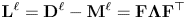
(5)\begin{equation} \mathbf{L}^\ell = \mathbf{D}^\ell - \mathbf{M}^\ell = \mathbf{F} \mathbf{\Lambda} \mathbf{F}^\top \end{equation}

where $\mathbf {D}^\ell$ is the diagonal degree matrix of $\mathbf {M}^\ell$. Consider a vector $\mathbf {s}\in \mathbb {R}^b$, we define $\hat {\mathbf {s}}$ the graph Fourier transform of $\mathbf {s}$ on $G^\ell$ as [Reference Shuman, Narang, Frossard, Ortega and Vandergheynst25]:

(6)\begin{equation} \hat{\mathbf{s}} = \mathbf{F}^\top \mathbf{s}. \end{equation}

Assume the order of the eigenvectors ($\mathbf {F}$) is chosen so that the corresponding eigenvalues are in ascending order. If only the first few entries of $\hat {\mathbf {s}}$ are nonzero then $\mathbf {s}$ is low frequency (smooth). In the extreme case where only the first entry of $\hat {\mathbf {s}}$ is nonzero we have that $\mathbf {s}$ is constant (maximum smoothness). From this definition we derive a measure called smoothness $\sigma ^\ell (\mathbf {s})$ of a signal $\mathbf {s}$. The smoothness is measured using the Laplacian quadratic form:

(7)\begin{equation} \sigma^\ell(\mathbf{s}) = \mathbf{s}^\top \mathbf{L}^\ell \mathbf{s} = \sum_{i,j = 1}^{b}{\mathbf{M}^\ell[i,j](\mathbf{s}[i] - \mathbf{s}[j])^2} \end{equation}

where we note that $\mathbf {s}$ is smoother when $\sigma ^\ell (\mathbf {s})$ is smaller.

In this paper we are particularly interested in smoothness of the label signals. We call label signal $\mathbf {s}_c$ associated with class $c$ a binary ($\{0,1\}$) vector whose nonzero coordinates are the ones corresponding to input vectors of class $c$. In other words, for any $i$, $1\leq i\leq b$:

(8)\begin{equation} \mathbf{s}_c[i] = 1 \Leftrightarrow (\mathbf{x}_i \; \text{is in class c} ). \end{equation}

From equation (7), we can see that the smoothness of label signal $\mathbf {s}_c$ is the sum of similarities between examples in distinct classes (since $(\mathbf {s}[i] - \mathbf {s}[j])$ is zero when $i$ and $j$ have the same label). Thus, a total smoothness of 0 means that all examples in distinct classes have 0 similarity.

Next we introduce a regularizer that limits how much $\sigma ^\ell$ can vary from one layer to the next, thus leading to a network that is more in line with Property 1. This will be shown to improve robustness in Section III.

D) Proposed regularizer

1) Definition

We propose to measure the deformation induced by a given layer $\ell$ by computing the difference between label signal smoothness before and after the layer for all labels:

(9)\begin{equation} \delta_\sigma^\ell = \sum_c{\left|\sigma^\ell(\mathbf{s}_c) - \sigma^{\ell-1}(\mathbf{s}_c)\right|}.\end{equation}

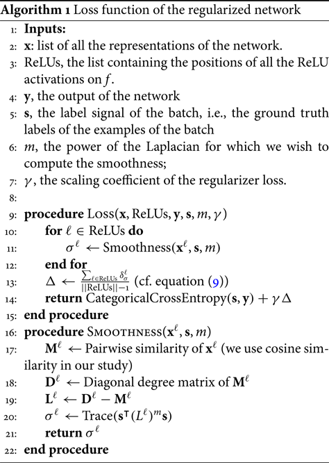
These quantities are used to regularize modifications made by each of the layers during the learning process. The pseudo-code of Algorithm 1 describes how we use the proposed regularizer to compute the loss.

Illustrative example:

In Fig. 1 we depicted a toy illustrative example to motivate the proposed regularizer. We consider here a one-dimensional two-class problem. To linearly separate circles and crosses, it is necessary to group all circles. Without regularization the resulting embedding is likely to either considerably increase the distance between examples in different classes (case (a)), thus producing sharp transitions in the network function, or to reduce the margin (case (b)). In contrast, by penalizing large variations of the smoothness of label signals (case (c)), the average distance between examples in different classes must be preserved in the embedding domain, resulting in a more precise control of distances within the boundary region.

Remark 1 Since we only consider label signals, we solely depend on the similarities between examples of distinct classes. As such, the regularizer only focuses on the boundary, and does not vary if the distance between examples of the same label grows or shrinks.

Remark 2 Compared with [Reference Cisse, Bojanowski, Grave, Dauphin and Usunier11], there are key differences that characterize the proposed regularizer:

(i) Only pairwise distances between examples are taken into account. This has the effect of controlling space deformations only in the directions of training examples.
(ii) The network is forced to maintain a minimum margin by keeping the smoothness small at each layer of the architecture, thus controlling both contraction and dilatation of space at the boundary. This is illustrated in Fig. 1, where [Reference Cisse, Bojanowski, Grave, Dauphin and Usunier11] is represented by b) and our method by c).
(iii) The proposed criterion is an average (sum) over all distances, rather than a stricter criterion (e.g. maintaining a small Lipschitz constant), which would force each pair of vectors $(\mathbf {x}_i, \mathbf {x}_j)$ to obey the constraint.

In summary, by enforcing small variations of smoothness across the layers of the network, the proposed regularizer maintains a large enough $r$ so that equation (3) can hold, while also controlling dilatation. Combining it with Parseval [Reference Cisse, Bojanowski, Grave, Dauphin and Usunier11] would allow for a better control of the $\alpha$ parameter in the other directions of the input space.

E) Relations to label signal bandwidth and powers of the Laplacian

Recent study [Reference Anis, ElGamal, Avestimehr and Ortega17] develops an asymptotic analysis of the bandwidth of label signals, $BW(\mathbf {s})$, where bandwidth is defined as the highest non-zero graph frequency of $\mathbf {s}$, i.e. the nonzero entry of $\hat {\mathbf {s}}$ with the highest index. An estimate of the bandwidth can be obtained by computing:

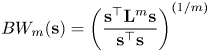
(10)\begin{equation} BW_m(\mathbf{s}) = \left( \frac{\mathbf{s}^{\top}\mathbf{L}^m \mathbf{s}}{\mathbf{s}^{\top}\mathbf{s}} \right)^{(1/m)} \end{equation}

for large $m$. This can be viewed as a generalization of the smoothness metric of (7). Anis et al. [Reference Anis, ElGamal, Avestimehr and Ortega17] show that, as the number of labeled points $\mathbf {x}$ (assumed drawn from a distribution $p(\mathbf {x})$) grows asymptotically, the bandwidth of the label signal converges in probability to the supremum of $p(\mathbf {x})$ in the region of overlap between classes. This motivates our study in three ways.

First, it provides theoretical justification to use $\sigma ^\ell (\mathbf {s})$ for regularization, since lower values of $\sigma ^\ell (\mathbf {s})$ are indicative of better separation between classes. Second, the asymptotic analysis suggests that using higher powers of the Laplacian would lead to better regularization, since estimating bandwidth using $BW_m(\mathbf {s})$ becomes increasingly accurate as $m$ increases. Finally, our regularization can be seen to be protective against specializing by preventing $\sigma ^\ell (\mathbf {s})$ from decreasing “too fast.” For most problems of interest, given a sufficiently large amount of labeled data available, it would be reasonable to expect the bandwidth of $\mathbf {s}$ not to be arbitrarily small, because the classes cannot be exactly separated, and thus a network that reduces the bandwidth too much could be unreliable (i.e. biased by the training set). After trying multiple values of $m$, we found that using $m=2$ usually led to close to the best performance in our experiments.

III. EXPERIMENTS

In the following subsections, we evaluate the proposed method using various tests. We use the well-known CIFAR-10 dataset [Reference Krizhevsky and Hinton26] as a first benchmark and we demonstrate that our proposed regularizer can improve robustness as defined in Section II.A.

In summary, in subsection A) we first verify that the proposed regularizer favors Definition 1. We then show in subsection B) that by using the proposed regularizer we are able to increase robustness for random perturbations and weak adversarial attacks. In subsection C), we challenge our method on more competitive benchmarks. Finally, in subsection D) we extend the analysis to CIFAR-100 [Reference Krizhevsky and Hinton26] and Imagenet32x32 [Reference Chrabaszcz, Loshchilov and Hutter27] to validate the generality of the method. These experiments demonstrate that DNNs trained with the proposed regularizer lead to improved robustness.

To measure accuracy, we average over 10 runs each time, unless mentioned otherwise. In all reports, $P$ stands for Parseval [Reference Cisse, Bojanowski, Grave, Dauphin and Usunier11] trained networks, $R$ for networks trained with the proposed regularizer, and $V$ for Vanilla (i.e. baseline) networks. Note that the network architecture is the same for all networks and that Vanilla refers to the network architecture trained without any regularizer. The network architecture is depicted in Fig. A1. Training hyperparameters and details of our implementation of the Parseval method can be found in the Appendix. The corresponding code is available at https://github.com/cadurosar/laplacian_networks.

A) Robustness of trained architectures

First we verify that the proposed regularizer improves robustness as defined in Section II.A. For various values of $r$, we estimate $\alpha _{\min }(r) = \arg \min _{\alpha }{\{\,f\in Robust_{\alpha }(r)\}}$. We use 1000 training examples and generate 100 uniform noises to estimate $\alpha _{\min }(\cdot )$. Results are shown in Fig. 2. We observe that networks trained with the proposed regularizer allow for smaller $\alpha$ values when the radius $r$ increases. The Parseval method achieves better Lipschitz constant than Vanilla, as suggested by the large values of $r$. However, we observe that $\alpha _{\min }$ grows fast when using Parseval, suggesting that sharp transitions are allowed in the vicinity of trained examples.

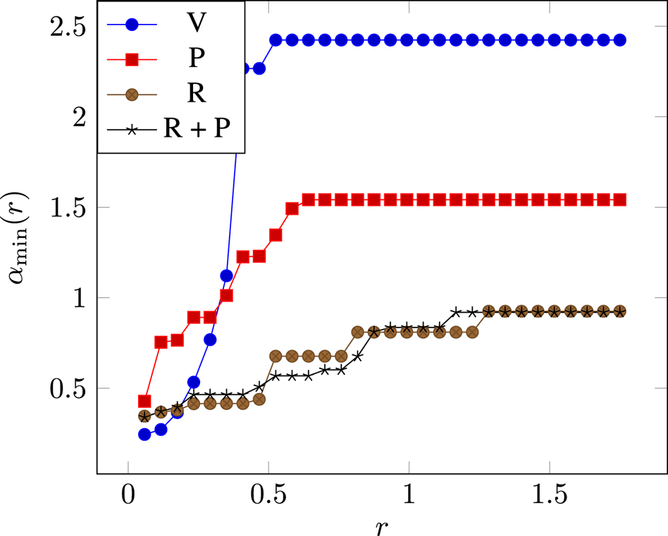
Fig. 2. Estimations of $\alpha _{\min }(r)$ obtained for different radii $r$ over training examples. The proposed regularizer allows for smaller $\alpha$ values when $r$ increases.

B) Experiments on perturbations and adversarial attacks

In this subsection we verify the ability of the proposed regularizer to increase robustness, while retaining acceptable accuracy on the clean test set, on the CIFAR-10 dataset without any type of data augmentation.

1) Clean test set

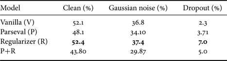
Before checking the robustness of the network, we first test the performance on clean examples. In the second column of Table 1, we show the baseline accuracy of the models on the clean CIFAR-10 test set (no perturbation is added at this point). These experiments agree with the claim from [Reference Cisse, Bojanowski, Grave, Dauphin and Usunier11] where the authors show that they are able to increase the performance of the network on the clean test set. We observe that the proposed method leads to a minor decrease of performance on this test. However, we see in the following experiments that this is compensated by an increased robustness to perturbations. The fact that it is difficult to avoid such a trade-off between robustness and accuracy has already been discussed in the literature [Reference Fawzi, Fawzi and Frossard28].

Table 1. Network mREI under different types of perturbations

Bottom line represents the corresponding median Cosine Distance (mCD) (at the highest perturbation severity) between corrupted and clean images.

2) Perturbation robustness

In order to assess the effectiveness of the various methods when subject to perturbations, we use the benchmark proposed in [Reference Hendrycks and Dietterich7] which consists of 15 different perturbations, with five levels of severity each (note that they are referred to as “corruptions” in [Reference Hendrycks and Dietterich7]). Perturbations test the robustness of the network to noise when compared to its clean test set performance. We illustrate each perturbation in Fig. 3.

Fig. 3. Illustration of the 15 perturbations from [Reference Hendrycks and Dietterich7]. Best viewed in color.

In more detail, we are interested in the mean relative error inflation (mREI). To define it, consider $E^{\texttt {per},\texttt {sev}}_{\texttt {net}}$ the error rate of a network net (V,P,R or P+R), under perturbation type per and severity sev. Denote $E_{\texttt {net}}$ the error rate of the network $\texttt {net}$ on the clean set. We first define Error Inflation (EI) as:

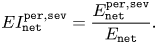
\[ EI_\texttt{net}^{\texttt{per},\texttt{sev}} = \frac{E^{\texttt{per},\texttt{sev}}_\texttt{net}}{E_\texttt{net}}. \]

Then the REI is defined as:

\[ REI_\texttt{net}^{\texttt{per},\texttt{sev}}= EI_\texttt{net}^{\texttt{per},\texttt{sev}} - EI_\texttt{V}^{\texttt{per},\texttt{sev}}. \]

Finally, mREI is obtained by averaging over all severities.

The results are described in Table 1 for the CIFAR-10 dataset. The raw error rates under each type of perturbation can be found in the Appendix. We observe that Parseval alone is not able to help with the mREI, despite reducing the clean set error. On the other hand, the proposed regularizer and its combination with Parseval training decreases the clean set accuracy but increases the relative performance under perturbations by a significant amount.

This experiment supports the fact that the proposed regularizer can significantly improve robustness to most types of perturbations introduced in [Reference Hendrycks and Dietterich7]. It is worth pointing out that this finding does not hold for Impulse Noise, Fog, and Contrast. Looking more into detail, we observe that Impulse noise shifts some values on the image to either its maximum possible value or the minimum possible value, while Fog and Contrast perform a re-normalization of the image. In those cases perturbations have the effect of creating noisy inputs that are far away (in terms of the cosine distance) from the original images, as supported by the last line of the table. This is in contrast to the other types of perturbations in the experiment. Because they can be far away, these perturbations do not fulfill the definition of equation (2), where there is a maximum radius $r$ for which robustness is enforced around the examples. In other words, our robustness definition is focusing on small deviations/distances as those are more likely to characterize noise (i.e we focus on distances that are too small to change the class of the image).

3) Adversarial robustness

We next evaluate robustness to adversarial inputs, which are specifically built to fool the network function. Such adversarial inputs can be generated and evaluated in multiple ways. Here we implement three approaches: first a mean case of adversarial noise, where the adversary can only use one forward and one backward pass to generate the perturbations, second a worst case scenario, where the adversary can use multiple forward and backward passes to try to find the smallest perturbation that will fool the network, third a compromise between the mean case and the worst case, where the adversary can do a predefined number of forward and backward passes with a perturbation threshold limit.

For the first approach, we add the scaled gradient sign (called the fast gradient signal method or FGSM) to the input [Reference Kurakin, Goodfellow and Bengio13], so that we obtain a target signal-to-noise ratio (SNR) of 33. This is in line with previous studies [Reference Cisse, Bojanowski, Grave, Dauphin and Usunier11]. Obtained results are introduced in the left and center plots of Fig. 4. In the left plot the noise is added after normalizing the input, whereas on the middle plot it is added before normalizing it. As with the perturbation tests, a combination of the Parseval method and our proposed approach yields the most robust architecture.

Fig. 4. Robustness against an adversary measured by the test set accuracy under FGSM attack in the left and center plots and by the mean $\mathcal {L}_2$ pixel distance needed to fool the network using DeepFool on the right plot.

With regard to the second approach, where a worst case scenario is considered, we use the Foolbox [Reference Rauber, Brendel and Bethge29] implementation of DeepFool [Reference Moosavi Dezfooli, Fawzi and Frossard14]. Due to time constraints we sample only ${1}/{10}$ of the test set images for this test. The conclusions we can draw are similar (right plot of Fig. 4) to those obtained for the first adversarial attack approach. Finally, for the third approach we use the PGD (projected gradient descent) attack introduced in [Reference Madry, Makelov, Schmidt, Tsipras and Vladu15]. PGD is an iterative version of FGSM, which loops for a maximum number of $it$ iterations. For each iteration it moves by a distance of $step$ in the direction of the gradient, provided it does not move away from the original image by a distance greater than $\epsilon$. Our experiments (described in Table 2) show that the proposed regularizer increases robustness against a PGD attack, for an epsilon corresponding to an SNR of about 33 ($it=20,step=0.002,\epsilon =0.01$).

Table 2. Median test set accuracy on the CIFAR-10 dataset against the PGD attack

A common pitfall in evaluating robustness to adversarial attacks comes from the fact the gradient of the architecture can be masked due to the introduced method. As a consequence, generated attacks become weaker compared to those on the vanilla architecture. So, to further verify that the obtained results are not only due to gradient masking, we perform tests with black box FGSM, where the target attacked network is not the same as the source of the adversarial noise. This way, all networks are tested against the same attacks.

For this test we continue to use an SNR of about 33 with the FGSM method. We choose the network with the best performance for each of the tested methods. The results are depicted in Table 3. In our experiments, we found that the combination of our method with Parseval is the most robust to noise coming from other sources. This demonstrates that the improvements are not caused by gradient masking, but are caused by the increased robustness of the proposed method and Parseval's. Interestingly, the noise created by both Parseval and our method did not challenge the other methods as well as the one created by Vanilla, justifying a posteriori the interest of this experiment.

Table 3. Comparison of CIFAR-10 test set accuracy under the black box FGSM attack

The most robust target for a given source is bolded, while the strongest source for a target is in italic.

4) Robustness to parameter and activation noises

In a third series of experiments we aim at evaluating the robustness of the architecture to noise on parameters and activations. We consider two types of noises: (i) erasures of the memory (dropout), and (ii) quantization of the weights [Reference Hubara, Courbariaux, Soudry, El-Yaniv and Bengio23].

In the dropout case, we compute the test set accuracy when the network has a probability of either $25$ or $40\%$ of dropping an intermediate representation value after each block of computation in the architecture. We average over a run of $40$ experiments. Results are depicted in the left and center plots of Fig. 5. It is interesting to note that the Parseval trained functions seem to collapse as soon as we reach $40\%$ probability of dropout, providing an average accuracy smaller than the vanilla networks. In contrast, the proposed method is the most robust to these perturbations.

Fig. 5. CIFAR-10 test set accuracy under different types of implementation related noise.

For the quantization of the weights, we aim at compressing the network size in memory by a factor of 6. We therefore quantize the weights using 5 bits (instead of 32) and re-evaluate the test set accuracy. The right plot of Fig. 5 shows that the proposed method is providing a better robustness to this perturbation than the tested counterparts.

Overall, these experiments confirm previous ones in the conclusion that the proposed regularizer obtains the best robustness compared to Parseval and Vanilla networks. Note that in this case (parameter and activation noise) there is a drop of performance when combining the proposed regularizer with the Parseval method. Although we do not have direct theoretical justification for this, the fact that the proposed regularizer and Parseval present conflicting strategies (smoothness versus contraction) could explain the drop in accuracy when the two methods are combined.

C) Experiments on challenging benchmarks

In this subsection we verify the ability of the proposed regularizer to increase robustness on the CIFAR-10 dataset while being combined with recent techniques of adversarial data augmentation. This is important as those methods are seen as the state of the art for adversarial robustness. Adversarial data augmentation consists of augmenting the training set during the training stage by using the same kind of attacks as those described in the last subsection. We refer to techniques using adversarial data augmentation using the letter A.

1) Tests with FGSM adversarial data augmentation

We first perform experiments with adversarial data augmentation as suggested in [Reference Kurakin, Goodfellow and Bengio13]. To be more precise we use the method they advise which is called “step1.1” using $\epsilon = {8}/{255}$.

A first test consists of measuring the accuracy when inputs are modified with additive Gaussian noise with various SNRs. As expected, we observe in Fig. 6 that training with adversarial examples helps in this case, as it adds more variation to the training set. Yet it reduces the accuracy on the clean set (left plot). Note that combining our method with adversarial training results in the best median accuracy.

Fig. 6. Test set accuracy under Gaussian noise with varying SNRs.

About robustness to adversarial attacks, the obtained results are depicted in Fig. 7. We observe that adding FGSM adversarial training does not generalize well to other types of attacks (which is readily seen in the literature [Reference Madry, Makelov, Schmidt, Tsipras and Vladu15]). Overall, the models using the proposed regularizer are the most robust again.

Fig. 7. Robustness against an adversary measured by the test set accuracy under FGSM attack in the left and center plots and by the mean $\mathcal {L}_2$ pixel distance needed to fool the network using DeepFool on the right plot.

Finally, when considering implementation related perturbations, the results depicted in Fig. 8 are consistent with the ones from the previous section, in which is shown that the proposed regularizer helps improving robustness to this type of noise.

Fig. 8. Test set accuracy under different types of implementation related noise.

In summary, even when adding adversarial training, the proposed regularizer is either the most robust in median, or capable of improving the robustness when combined with the other methods.

2) Tests with PGD adversarial data augmentation

Most of our adversarial tests are performed with FGSM because of its simplicity and speed, even though it has already been shown (e.g. [Reference Madry, Makelov, Schmidt, Tsipras and Vladu15]) that FGSM is weak as an attack and as a defense mechanism. Despite the fact we do not only target adversarial defense, we further stress the ability of the proposed regularizer to improve it and to combine with other methods. To this end we perform experiments against the PGD attack.

As the proposed regularizer can be combined with FGSM defense, it is natural to also test it alongside PGD training. We use the parameters advised in [Reference Madry, Makelov, Schmidt, Tsipras and Vladu15]: seven iterations with $step = 2/255$, and $\epsilon =8/255$. The results depicted in Table 4 show that using our regularizer increases robustness of networks trained with PGD. Note that Dropout and Gaussian noise were applied 10 times to each of the networks and the results are displayed as the mean test set accuracy under these perturbations. A rate of 40% was used for dropout. The PGD attack uses the following parameters: $it=20,step={2}/{255},\epsilon ={8}/{255}$.

Table 4. Test set accuracy results on the CIFAR-10 dataset with PGD training

D) Experiments with other datasets

In this final subsection, we test the generality of the method using the CIFAR-100 and ImageNet32x32 datasets, with a subset of the perturbations used for CIFAR-10. Gaussian noise is applied 10 times to each of the networks for a total of 30 different runs. An SNR of $33$ is used for FGSM and $15$ for Gaussian noise. Images are normalized in the same way as the experiments with CIFAR-10. Standard data augmentation is used for CIFAR-100.

Results on CIFAR-100 are shown in Table 5 as the mean over three different initializations. We observe that as it was the case on CIFAR-10, the proposed method and the combination of the methods is the most robust on these test cases.

Table 5. Test set accuracy results on the CIFAR-100 dataset

We then use Imagenet32x32, a downscaled version of Imagenet [Reference Deng, Dong, Socher, Li, Li and Fei-Fei30] which can be used as an alternative to CIFAR-10 while maintaining a similar computational budget [Reference Chrabaszcz, Loshchilov and Hutter27]. We use the same network and training hyperparameters of the original paper. Further description can be found in the Appendix. Gaussian noise and Dropout are applied 40 times to each of the networks. Gaussian noise is applied with $SNR =33$ whereas Dropout is applied with 15%.

Results are shown in Table 6. We observe that as it was the case on CIFAR-10 and CIFAR-100, the proposed method provides more robustness in all of these test cases. Note that we had trouble fine-tuning the $\beta$ parameter for the Parseval criterion, explaining the poor performance of Parseval and its combination with our proposed regularizer.

Table 6. Test set accuracy results on the Imagenet32x32 dataset

IV. CONCLUSION

In this paper we have introduced a definition of robustness alongside an associated regularizer. The former takes into account both small variations around the training set examples and the margin. The latter enforces small variations of the smoothness of label signals on similarity graphs obtained at intermediate layers of a DL network architecture. We have empirically shown with our tests that the proposed regularizer can lead to improved robustness in various conditions compared to existing counterparts. We also demonstrated that combining the proposed regularizer with existing methods can result in even better robustness for some conditions.

Future study includes a more systematic study of the effectiveness of the method with regards to other datasets, models, and perturbations. Recent studies have shown that adversarial noise is partially transferable between models and dataset [Reference Moosavi-Dezfooli, Fawzi, Fawzi and Frossard31, Reference Papernot, McDaniel and Goodfellow32] and therefore we are confident about the generality of the method in terms of models and datasets.

FINANCIAL SUPPORT

This study was funded in part with the support of Région Bretagne and computations were performed with the use of Nvidia GPUs, courtesy of Nvidia.

CONFLICT OF INTEREST

None.

APPENDIX

P A R S E V A L T R A I N I N G

We compare our results with those obtained using the method described in [Reference Cisse, Bojanowski, Grave, Dauphin and Usunier11]. There are three modifications to the normal training procedure: orthogonality constraint, convolutional renormalization, and convexity constraint.

For the orthogonality constraint we enforce Parseval tightness [Reference Kovačević and Chebira33] as a layer-wise regularizer:

(A.1)\begin{equation} R_\beta(W^\ell) = \frac{\beta}{2}\|W^{\ell\top} W^\ell - I\|^2_2,\end{equation}

where $W_\ell$ is the weight tensor at layer $\ell$. This function can be approximately optimized with gradient descent by doing the operation:

(A.2)\begin{equation} W^\ell \leftarrow (1 + \beta)W^\ell - \beta W^\ell W^{\ell\top} W^\ell.\end{equation}

Given that our network is smaller we can apply the optimization to the entirety of the $W$, instead of $30\%$ as per the original paper, this increases the strength of the Parseval tightness.

For the convolutional renormalization, each matrix $W^\ell$ is reparameterized before being applied to the convolution as ${W^\ell }/{\sqrt {2k_lk_w +1}}$, where $k_w$ is the kernel width and $k_h$ is the kernel height.

For our architecture the inputs from a layer come from either one or two different layers. In the case where the inputs come from only one layer, $\alpha$ the convexity constraint parameter is set to 1. When the inputs come from the sum of two layers we use $\alpha = 0.5$ as the value for both of them, which constraints our Lipschitz constant, this is softer than the convexity constraint from the original paper.

H Y P E R P A R A M E T E R S

We train our networks using classical stochastic gradient descent with momentum ($0.9$), with batch size of $b=100$ images and using a L2-norm weight decay with a coefficient of $\lambda = 0.0005$.

We use the mean of the difference of smoothness between successive layers in our loss function. Therefore in our loss function we have:

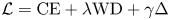
(A.3)\begin{equation} \mathcal{L} = \text{CE} + \lambda \text{WD} + \gamma\Delta\end{equation}

where $\Delta = ({1}/({d-1})) \sum _{\ell =1}^d | \delta _\sigma ^\ell |$, CE is the cross entropy function and WD is weight decay.

CIFAR-10

For the CIFAR-10 dataset we do a 100 epoch training. Our learning rate starts at $0.1$. After half of the training ($50$ epochs) the learning rate decreases to $0.001$. We do not add data augmentation, as it can interfere with some of the perturbations (elastic transformations for example).

We tested multiple parameters of $\beta$, the Parseval tightness parameter, $\gamma$ the weight for the smoothness difference cost, and $m$ the power of the Laplacian. We found that the best values for this specific architecture, dataset, and training scheme were: $\beta = 0.01, \gamma = 0.0001, m = 2$. The PreActResNet18 network depicted in Fig. A1 is used in all experiments for CIFAR-10.

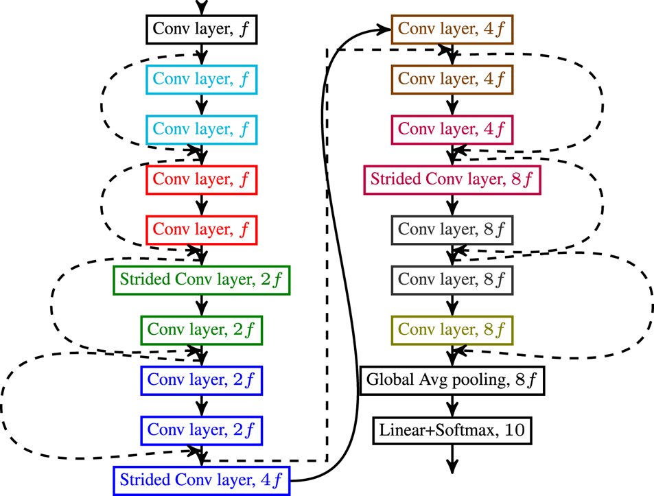
Fig. A1. Depiction of the studied network.

CIFAR-100

We perform experiments using the WideResNet28-10 [Reference Zagoruyko and Komodakis34] architecture, and we added standard data augmentation (random crops and random horizontal flipping) and dropout with probability of $30\%$ after the first convolution of each residual block. We train for 200 epochs, starting with a learning rate of 0.1 and divide the learning rate by 5 in epochs 60, 120, and 160. Momentum of 0.9 is used and weight decay of $5\times 10^{-4}$.

We tested multiple parameters of $\beta$, the Parseval tightness parameter, $\gamma$ the weight for the smoothness difference cost, and $m$ the power of the Laplacian. We found that the best values for this specific architecture, dataset and training scheme were: $\beta = 0.0003, \gamma = 0.01, m = 2$. FGSM is applied after normalization of the input.

IMAGENET32x32

We perform experiments using the WideResNet28-5 [Reference Zagoruyko and Komodakis34] architecture, and we added standard data augmentation (random crops and random horizontal flipping). We follow the training procedure from [Reference Chrabaszcz, Loshchilov and Hutter27], where training is done for 30 epochs, starting with a learning rate of 0.1 and divide the learning rate by 5 in epochs 10 and 20. Momentum of 0.9 is used and weight decay of $5\times 10^{-4}$.

We tested multiple parameters of $\beta$, the Parseval tightness parameter, $\gamma$ the weight for the smoothness difference cost, and $m$ the power of the Laplacian. We found that the best values for this specific architecture, dataset and training scheme were: $\beta = 10^{-6}, \gamma = 0.01, m = 2$.

D E P I C T I O N O F T H E N E T W O R K

Figure A1 depicts the network we call PreActResNet18, $f=64$ is the filter size of the first layer of the network. Conv layers are $3\times 3$ layers and are always preceded by batch normalization and ReLU (except for the first layer which receives just the input). The smoothness is calculated after each ReLU.

P E R T U R B A T I O N R O B U S T N E S S

Table A1 contains the mean test error under each type of perturbation.

Table A1. Networks error under different types of perturbations

T I M E R E Q U I R E D T O T R A I N T H E N E T W O R K S

The proposed regularizer requires the computation of a similarity matrix and therefore increases the overall training time. The same happens for the other methods that we compare to in this study (Parseval, FGSM, and PGD trainings).

To better understand the impact of each considered method on the training time, we report in Table A2 the training times. We note that the proposed regularizer has a greater computation cost than the Parseval method, but it is significantly faster than the adversarial training methods. Overall, the added training time of the proposed regularizer remains very limited.

Table A2. Comparison of the total time that it takes to train each method

Carlos Lassance received an engineering double-degree from PUC-Rio and IMT Atlantique in 2017, and he received his Ph.D. degree in machine learning and graphs from IMT Atlantique in 2020. He was recently an intern at Mila (2018–19) and started reviewing for IEEE journals. His main research interests are GSP and deep neural networks.

Vincent Gripon is a permanent researcher with IMT Atlantique, a French top technical university. He obtained his M.S. from École Normale Supérieure Paris-Saclay in 2008 and his Ph.D. from IMT Atlantique in 2011. He spent 1 year as a visiting scientist at McGill University between 2011 and 2012 and 1 year as an invited Professor at Mila and Université de Montréal. His research mainly focuses on efficient implementation of artificial neural networks, graph signal processing, deep learning robustness and associative memories. He has co-authored more than 70 papers in these domains in prestigious venues.

Antonio Ortega received his undergraduate and doctoral degrees from the Universidad Politécnica de Madrid, Madrid, Spain and Columbia University, New York, NY, respectively. In 1994 he joined the Electrical and Computer Engineering department at the University of Southern California (USC), where he is currently a Professor and has served as Associate Chair. He is a Fellow of the IEEE and EURASIP, and a member of ACM and APSIPA. He was the inaugural Editor-in-Chief (EiC) of the APSIPA Transactions is the EiC of the IEEE Transactions of Signal and Information Processing over Networks. He recently served as a member of the Board of Governors of the IEEE Signal Processing Society. He has received several paper awards, including the 2016 Signal Processing Magazine award. His recent research work is focusing on graph signal processing, machine learning, multimedia compression, and wireless sensor networks. Over 40 Ph.D. students have completed their thesis under his supervision and his work has led to over 400 publications in international conferences and journals, as well as several patents.

Footnotes

¹ Note that the distance between any two examples at a certain layer depends on their positions in the original domain and the network function applied up to that layer. Thus, constraints on the distances lead to constraints on the parameters of the network function.

References

REFERENCES

He, K.; Zhang, X.; Ren, S.; Sun, J.: Identity mappings in deep residual networks, in European Conference on Computer Vision, Springer, 2016, 630–645.CrossRef Google Scholar

Wu, Y.; Schuster, M.; Chen, Z.; Le, Q.V.; Norouzi, M.; Macherey, W.; Krikun, M.; Cao, Y.; Gao, Q.; Macherey, K., et al. : Google's neural machine translation system: Bridging the gap between human and machine translation. arXiv preprint arXiv:1609.08144, 2016.Google Scholar

LeCun, Y.; Bengio, Y.; Hinton, G.: Deep learning. Nature, 521 (7553) (2015), 436.CrossRef Google Scholar PubMed

Szegedy, C. et al. .: Intriguing properties of neural networks. arXiv preprint arXiv:1312.6199, 2013.Google Scholar

Goodfellow, I.J.; Shlens, J.; Szegedy, C.: Explaining and harnessing adversarial examples. arXiv preprint arXiv:1412.6572, 2014.Google Scholar

Gilmer, J.; Adams, R.P.; Goodfellow, I.; Andersen, D.; Dahl, G.E.: Motivating the rules of the game for adversarial example research. arXiv preprint arXiv:1807.06732, 2018.Google Scholar

Hendrycks, D.; Dietterich, T.: Benchmarking neural network robustness to common corruptions and perturbations. Proceedings of the International Conference on Learning Representations, 2019.Google Scholar

Papernot, N.; McDaniel, P.D.: Deep $k$

-nearest neighbors: Towards confident, interpretable and robust deep learning. CoRR, vol. abs/1803.04765, 2018.Google Scholar

Gu, S.; Rigazio, L.: Towards deep neural network architectures robust to adversarial examples. arXiv preprint arXiv:1412.5068, 2014.Google Scholar

Mallat, S.: Understanding deep convolutional networks. Phil. Trans. R. Soc. A, 374 (2065) (2016), 20150203.CrossRef Google Scholar PubMed

Cisse, M.; Bojanowski, P.; Grave, E.; Dauphin, Y.; Usunier, N.: Parseval networks: improving robustness to adversarial examples, in International Conference on Machine Learning, 2017, 854–863.Google Scholar

Pezeshki, M.; Fan, L.; Brakel, P.; Courville, A.; Bengio, Y.: Deconstructing the ladder network architecture, in International Conference on Machine Learning, 2016, 2368–2376.Google Scholar

Kurakin, A.; Goodfellow, I.; Bengio, S.: Adversarial machine learning at scale. arXiv preprint arXiv:1611.01236, 2016.Google Scholar

Moosavi Dezfooli, S.M.; Fawzi, A.; Frossard, P.: Deepfool: a simple and accurate method to fool deep neural networks, in Proceedings of 2016 IEEE Conference on Computer Vision and Pattern Recognition (CVPR), 2016.CrossRef Google Scholar

Madry, A.; Makelov, A.; Schmidt, L.; Tsipras, D.; Vladu, A.: Towards deep learning models resistant to adversarial attacks, in International Conference on Learning Representations, 2018.Google Scholar

Gripon, V.; Ortega, A.; Girault, B.: An inside look at deep neural networks using graph signal processing, in Proceedings of ITA, February 2018.CrossRef Google Scholar

Anis, A.; ElGamal, A.; Avestimehr, S.; Ortega, A.: A sampling theory perspective of graph-based semi-supervised learning. IEEE Transactions on Information Theory, 65 (4) (2019), 2322–2342. doi:10.1109/TIT.2018.2879897.CrossRef Google Scholar

Lassance, C.; Gripon, V.; Tang, J.; Ortega, A.: Structural robustness for deep learning architectures, in 2019 IEEE Data Science Workshop (DSW), June 2019, 125–129.CrossRef Google Scholar

Lassance, C.E.R.K.; Gripon, V.; Ortega, A.: Laplacian power networks: Bounding indicator function smoothness for adversarial defense’. CoRR, vol. abs/1805.10133, 2018.Google Scholar

Anirudh, R.; Thiagarajan, J.J.; Sridhar, R.; Bremer, T.: Influential sample selection: A graph signal processing approach’. arXiv preprint arXiv:1711.05407, 2017.Google Scholar

Svoboda, J.; Masci, J.; Monti, F.; Bronstein, M.M.; Guibas, L.: Peernets: Exploiting peer wisdom against adversarial attacks’. arXiv preprint arXiv:1806.00088, 2018.Google Scholar

Bronstein, M.M.; Bruna, J.; LeCun, Y.; Szlam, A.; Vandergheynst, P.: Geometric deep learning going beyond Euclidean data. IEEE Signal Process. Mag., 34 (4) (2017), 18–42.CrossRef Google Scholar

Hubara, I.; Courbariaux, M.; Soudry, D.; El-Yaniv, R.; Bengio, Y.: Quantized neural networks Training neural networks with low precision weights and activations. J. Mach. Learn. Res., 18 (2017), 187–1.Google Scholar

Goodfellow, I.; Bengio, Y.; Courville, A.: Deep learning, 1, MIT Press, Massachusetts, USA, 2017.Google Scholar

Shuman, D.I.; Narang, S.K.; Frossard, P.; Ortega, A.; Vandergheynst, P.: The emerging field of signal processing on graphs. Extending high-dimensional data analysis to networks and other irregular domains. IEEE Signal Process. Mag., 30 (3) (2013), 83–98.CrossRef Google Scholar

Krizhevsky, A.; Hinton, G.: Learning multiple layers of features from tiny images. https://www.cs.toronto.edu/kriz/learning-features-2009-TR.pdf, 2009.Google Scholar

Chrabaszcz, P.; Loshchilov, I.; Hutter, F.: A downsampled variant of imagenet as an alternative to the CIFAR datasets. arXiv preprint arXiv:1707.08819, 2017.Google Scholar

Fawzi, A.; Fawzi, O.; Frossard, P.: Analysis of classifiers’ robustness to adversarial perturbations. Mach. Learn., 107 (3) (2018), 481–508.CrossRef Google Scholar

Rauber, J.; Brendel, W.; Bethge, M.: Foolbox: a python toolbox to benchmark the robustness of machine learning models. arXiv preprint arXiv:1707.04131, 2017.Google Scholar

Deng, J.; Dong, W.; Socher, R.; Li, L.-J.; Li, K.; Fei-Fei, L.: ImageNet: a Large-Scale Hierarchical Image Database, in CVPR09, 2009.CrossRef Google Scholar

Moosavi-Dezfooli, S.-M.; Fawzi, A.; Fawzi, O.; Frossard, P.: Universal adversarial perturbations. arXiv preprint, 2017.CrossRef Google Scholar

Papernot, N.; McDaniel, P.; Goodfellow, I.: Transferability in machine learning: from phenomena to black-box attacks using adversarial samples. arXiv preprint arXiv:1605.07277, 2016.Google Scholar

Kovačević, J.; Chebira, A.: An introduction to frames. Found. Trends Signal Process., 2 (1) (2008), 1–94.CrossRef Google Scholar

Zagoruyko, S.; Komodakis, N.: Wide residual networks. arXiv preprint arXiv:1605.07146, 2016.Google Scholar

Fig. 2. Estimations of $\alpha _{\min }(r)$ obtained for different radii $r$ over training examples. The proposed regularizer allows for smaller $\alpha$ values when $r$ increases.