


I. INTRODUCTION
Recently, the area of deep learning is booming owing to the availability of high computation GPGPU and ability to process massive data. Many state-of-the-art performances have been achieved with deep learning for different tasks, including image classification[Reference Deng, Dong, Socher, Li, Li and Fei-Fei1], object detection [Reference Everingham, Van Gool, Williams, Winn and Zisserman2], and semantic segmentation [Reference Cordts3], and new tasks such as iterative reconstruction [Reference Choy, Xu, Gwak, Chen and Savarese4] and depth estimation [Reference Silberman, Hoiem, Kohli and Fergus5]. However, when neural networks become deeper and wider, the complexity of deep neural network (DNN) models grows rapidly. Consequently, DNN models cannot practically work with a large number of parameters and high levels of computation, notably for Internet of Things (IoT) devices and self-driving car (Autonomous car).
There are five approaches to achieve a compact yet accurate model–frugal architecture, pruning, matrix decomposition, quantization, and specialist knowledge distillation (KD). KD is researched to understand how to train a student deep neural network (S-DNN) by learning from teacher deep neural network (T-DNN). In general, S-DNN does not have the same layers as T-DNN; thus, it is difficult to train to find the optimization point. There are two branches of KD approaches. One is the conventional approach, referred to as offline methods [Reference Yim, Joo, Bae and Kim6–Reference Park, Kim, Lu and Cho11], which train the T-DNN first, then use the S-DNN to mimic the pre-trained T-DNN. Although this two-phase approach incurs considerable computation time, we get a better performing S-DNN. Sometimes, this S-DNN is better performing than the pre-trained T-DNN, because the T-DNN is already pre-trained and has more layers than the S-DNN, while the S-DNN has a better initial weight. The other approach is referred to as online methods [Reference Zhang, Xiang, Hospedales and Lu12–Reference Lan, Zhu and Gong14], which start both as scratch models that train together. This one-phase approach expects to train a better model than when only training the S-DNN model. Compared with the offline methods, these online methods do not need to train a T-DNN first, so there is less training time. However, in this research, we are focused on how to get a better performing S-DNN model with the same compression rate. Because most of the conventional methods showed better results in experiments, we decided to pick the first method in this paper.
After considering the training method, what is taught from the pre-trained model as knowledge to the S-DNN model is very sensitive to its performance. To address this, FSP [Reference Yim, Joo, Bae and Kim6] proposed to use the correlation between input and output feature maps of the layer module, in the form of a Gramian matrix.
In this work, our contributions are as follows:
1) We propose a cross-layer matrix to extract more knowledge and add Kullback Leibler (KL) Divergence and offline ensemble to improve image classification with the same compression.
2) We propose $1\times 1$
 convolutional layers to tune the channels of T-DNN to be identical to those of S-DNN to solve the constraints of our proposed method.
3) We propose using two-step KD to improve image classification when there is a huge difference in layers between T-DNN and S-DNN, to avoid the loss of KD.
4) Our method can be used not only for image classification tasks [Reference Krizhevsky, Sutskever and Hinton15, Reference Simonyan and Zisserman16] but also for other tasks, such as object detection [Reference Ren, He, Girshick and Sun17, Reference Redmon and Farhadi18], semantic segmentation [Reference Liu, Chen, Liu, Qin, Luo and Wang19], and action estimation [Reference Ji, Xu, Yang and Yu20] in videos.

II. RELATED WORK
The compression methods can be divided into four categories, knowledge distillation, pruning, low-rank decomposition, and quantization.
A) Knowledge distillation
Hinton et al. [Reference Hinton, Vinyals and Dean7] distilled knowledge from a very large teacher model to promote a small student model by using a softened softmax of a teacher network. The rationale is to take advantage of extra supervision provided by the teacher model during the training of the student model, beyond a conventional supervised learning objective such as the cross-entropy loss subject to the training data labels. Romero et al. [Reference Romero, Ballas, Kahou, Chassang, Gatta and Bengio8] proposed “Hint training” to train partial layers, then used the final output layers to train the student model to enhance the performance. Park et al. [Reference Park, Kim, Lu and Cho11] proposed to transfer mutual relations of data examples. Yim et al. [Reference Yim, Joo, Bae and Kim6] transferred knowledge from the T-DNN to the S-DNN as output feature maps rather than as layer parameters. They become a certain layer group in the network and define the correlation between the input and output feature maps of the layer group as a Gram matrix so that the feature correlations of the S-DNN and T-DNN become similar. We expand the Gram matrix by adding more than cross-one layer. Furthermore, approach taken by Lee et al. [Reference Lee, Kim and Song10] is based on the correlation between two feature maps as knowledge by using Singular Value Decomposition (SVD). However, this approach [Reference Lee, Kim and Song10] will cost a significant computation time because feature maps that are needed to be decomposed by CPU. As a result, we take FSP [10] model as a baseline to enhance as our proposed methods.
Moreover, while earlier distillation methods often take an offline learning strategy that need two phases of the training procedure, the more recently proposed deep learning [Reference Zhang, Xiang, Hospedales and Lu12] method overcomes this limitation by conducting an online distillation in one-phase training between two peer student models. We will add KLDivergence in our proposed method, which makes it different than online methods. Anil et al. [Reference Anil, Pereyra, Passos, Ormandi, Dahl and Hinton13] extend [Reference Zhang, Xiang, Hospedales and Lu12] to decrease the training time of large-scale distributed neural networks. Lan et al. [Reference Lan, Zhu and Gong14] present an On-the-fly Native Ensemble (ONE) learning strategy for one-stage online distillation. However, existing online methods lack a strong “teacher” model, which limits the efficacy of knowledge discovery.
In [Reference Wang and Yoon21], Wang and Yoon provide a comprehensive survey on the recent progress of KD methods together with S-T frameworks typically used for vision tasks and systematically analyze the research status of KD in vision applications. KDGAN consisting of a classifier, a teacher, and a discriminator is proposed in [Reference Wang, Zhang, Sun and Qi22]. The classifier and the teacher learn from each other via distillation losses and are adversarially trained against the discriminator via adversarial losses. From the concrete distribution, continuous samples are generated to obtain low-variance gradient updates, which speed up the training. To efficiently transmit extracted useful teacher information to the student DNN, Bae et al. propose to perform bottom-up step-by-step transfer of densely distilled knowledge [Reference Bae, Yeo, Yim, Kim, Pyo and Kim23].
B) Deep neural network compression and efficient processing
Scientists found that network pruning can be used not only to reduce network complexity but also to prevent over-fitting. An old method [Reference Hanson and Pratt24] to pruning was the Biased Weight Decay. Han et al. [Reference Han, Pool, Tran and Dally25] first proposed that it's peaceful to remove neurons with zero input or output connections from the neural network. By using L1/L2 regularization, some of the weights converged to zeros after training. As a result, by using the combination of pruning, quantization, and Huffman coding [Reference Han, Mao and Dally26], the compression of AlexNet can reach 35$\times$ . CLIP-Q [Reference Tung and Mori27] flexibly makes weight pruning choices that can adapt to compress the DNN during the training time. Apart from weight pruning, there is another pruning approach, named channel pruning, that assesses neuron importance. Li et al. [Reference Li, Kadav, Durdanovic, Samet and Graf28] computed the importance of each filter by calculating its absolute weight sum. Furthermore, Hsiao et al.[Reference Hsiao, Chang, Chou and Chiu29] measured the significance of each filter by calculating the largest singular value.
In [Reference Deng, Li, Han, Shi and Xie30], Deng et al. provide a comprehensive survey on reviewing the mainstream compression approaches such as compacted model, tensor decomposition, data quantization, and network sparsification to compress DNN without compromising accuracy. In [Reference Sze, Chen, Yang and Emer31], Sze et al. present a tutorial and survey on understanding the key design for DNN and evaluating different DNN hardware implementations with benchmarks in order to achieve processing efficiency.
C) Low-rank decomposition
Low-rank approximation [Reference Denil, Shakibi, Dinh and De Freitas32–Reference Zhang, Zou, He and Sun35] approaches have been widely studied. However, low-rank approximation is inconvenient because each decomposition of feature maps is computationally expensive. Moreover, the methods of low-rank approximation only consider a few layers; therefore, they cannot consider the compression of the whole network.
D) Quantization
Quantization is a method for reducing the number of bits for weight and bias of each layer. We can divide methods either by using auxiliary data [Reference Basu and Varshney36, Reference Gupta, Agrawal, Gopalakrishnan and Narayanan37], or not using auxiliary data [Reference Dettmers38–Reference Ji, Ovsiannikov, Wang, Shi and Zhang40]. Additionally, there are two research approaches in compressing on bit-level. One is to use fixed-point implementation, and the other is to use common quantization methods, for example, K-means and scalar quantization. For fixed-point implementation, Hwang and Sung [Reference Hwang and Sung39] proposed a design with ternary weights, 3-bit signals, and an optimization process which was done by back-propagation-based re-training. For the other approach, Ji et al. [Reference Ji, Ovsiannikov, Wang, Shi and Zhang40] designed a supervised iteration quantization to reduce the bit resolution of the weights. They applied K-means-based adaptive quantization methods, such as vector quantization using K-means, product quantization, residual quantization, and discussed the efficacy of their design on compressing deep convolutional networks.
E) Deep learning
Special issues on deep learning framework architectures, hardware acceleration, DNN over the cloud, fog, edge, and end devices are elaborated [Reference Kang41]. In addition, methods and applications especially emphasizing on exploring recent advances in perceptual applications are addressed and discussed [Reference Kang41]. In [Reference Wang, Peng and Ko42], Wang et al. present to learn a proper prior from data for adversarial autoencoders. The notion of code generators is presented to transform manually selected simple priors into ones that can better characterize the data distribution.
III. PROPOSED ARCHITECTURE
The core idea of KD is how to define the vital information, then transfer the knowledge from the T-DNN to the S-DNN. As a result, we will divide our approach into four parts. Section A shows what the knowledge in T-DNN will transfer and its mathematical expression and the definition loss term $L_{KD}$ . Moreover, we will add another loss function $L_{KL}$
 between the prediction of T-DNN and S-DNN in Section B. Furthermore, we will use offline ensemble pre-trained T-DNNs to teach one student in Section C. Subsequently, the overall loss function will be discussed in Section Reference CordtsD. Finally, we will discuss the constraints of our proposed method and solutions. The overall architecture for our three proposed compression methods are shown in Fig. 1.
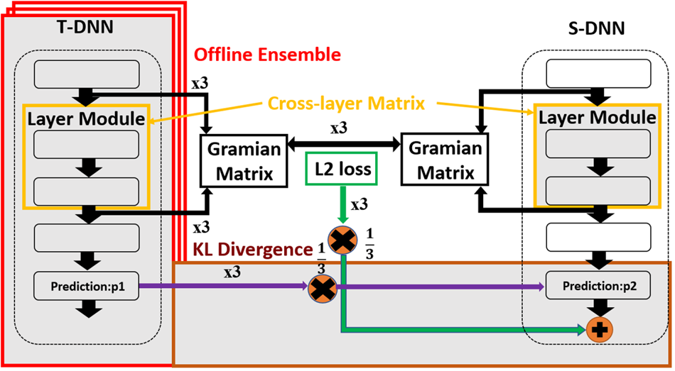
Fig. 1. Overall architecture of our proposed methods. There are three parts of our architecture. First, we propose cross-layer matrix to exact more features by FSP [Reference Yim, Joo, Bae and Kim6] adopting the proposed Gramian matrix in the orange part. Second, we adopt the KL Divergence in the offline environment to make S-DNN find a wider robust minimum in the brown part. Finally, we propose the use of offline ensemble pre-trained T-DNN to teach a S-DNN by using stochastic mean in the red part.
A) Cross-layer matrix
1) Proposed distilled knowledge
Yim et al. [Reference Yim, Joo, Bae and Kim6] proposed “FSP” by using Gramian matrix to mimic the generated features of the T-DNN, which can be a hard constraint for the S-DNN. Based on [Reference Yim, Joo, Bae and Kim6], we generate more Gramian matrices by crossing more than one layer. The numbers of cross matrices we add as loss function depends on how many layer modules are in DNN model. We believe that with more Gramian matrices in loss function, it would make the S-DNN get better performance.
The reason why we use the Gramian matrix created by feature maps is that we believe that instead of teaching the right answer to the student, it is better to teach the solution procedure to the student. Imagine there is a classroom, a teacher is teaching a student with a math question. It is better to teach how to use a formula first and the solution procedure than to provide the correct answer directly.
2) Mathematical expression of the knowledge distillation
Based on FSP [Reference Yim, Joo, Bae and Kim6], the Gramian matrix can be defined by two output feature maps. We propose the Gramian matrix as the knowledge to transfer. The Gramian matrix G $\mathbb {R}^{m \times n}$ is generated by the features from two layers. One output feature map is defined as $F^{1} \in \mathbb {R}^{h \times w \times m }$
 , where $h$
 , $w$
, $w$ , represent the height and width of output feature maps and $m$
 represents the number of output channels. The other output feature map is defined as $F^{2} \in \mathbb {R}^{h \times w \times n }$
 . Then, the Gramian matrix G $\mathbb {R}^{m \times n}$
 is calculated by (1)
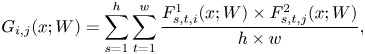
where $i,\,j$ represent the points of cross-one-layer results, $x$
 represents the input image and $W$
 are the weights of the network model. Unlike FSP [Reference Yim, Joo, Bae and Kim6], we select several points not only from cross-one module layer but also from cross-more-than-one module layer to generate more Gramian matrices as shown in (2) and (3).
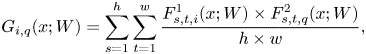
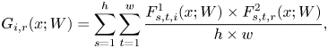
where $i,\,q$ represent the points of cross-two-layer results as shown in Fig. 2(b) and $i,\,r$
 represent the points of cross-three-layer results as shown in Fig. 2(c). In Fig. 2, we see there are three different kinds of cross-layer matrix. Our proposed method is to combine all the Gramian matrix 2(d) as knowledge.
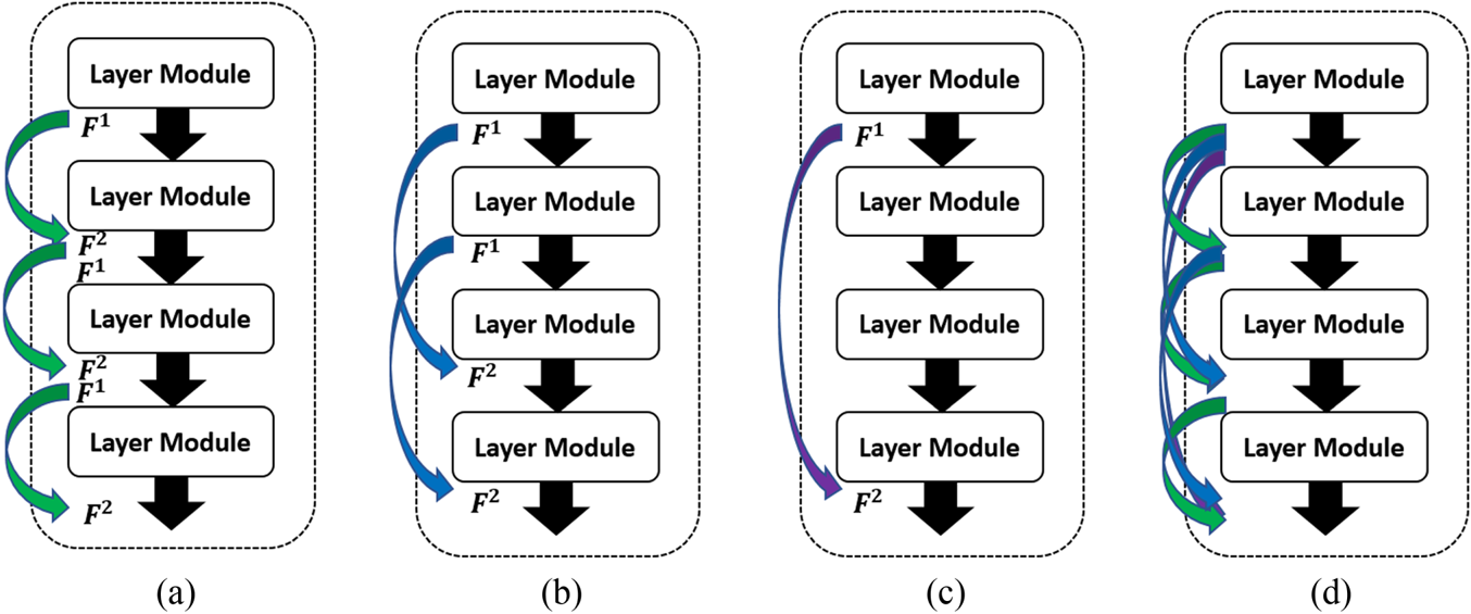
Fig. 2. (a) Cross one layer. (b) Cross two layers. (c) Cross three layers. (d) Our proposed.
3) KD loss for the Gramian matrix
As discussed previously, the T-DNN will teach S-DNN the solution of question by using the Gramian matrix. We assume that there are $B$ Gramian matrices $G_{b}^{T}$
 , $u=1,\,\ldots,\,B$
 , which are generated by the T-DNN, and $B$
 Gramian matrices $G_{b}^{S}$
 ,$i=1,\,\ldots,\,B$
 , which are generated by the S-DNN. Next, each pair of Gramian matrices will be calculated as the cost function by using the squared L2 norm. The cost function of knowledge distillation $L_{KD}(W_{t}; W_{s})$
 is defined as (4):

where $\lambda _{i}$ represents the weight for each KD loss and $B$
 represents the numbers of Gramian matrices. Because our proposed method adds more Gramian matrices by creating the cross matrices, we initially set all KD losses with the same weight. As a result, the values of $\lambda _{i}$
 are identical in our experiments.
B) KL Divergence
We propose using KL Divergence, which was used in DML [Reference Zhang, Xiang, Hospedales and Lu12], as our second-order loss function. In contrast to the online method [Reference Zhang, Xiang, Hospedales and Lu12] with two-direction learning, our offline method is only used in one direction from T-DNN to S-DNN. Given $D$ as the data examples $X={\{x_{n}\}_{n=1}^{D}}$
 from $C$
 classes, we represent the corresponding label set as $Y = \{ y_{i}\}_{n=1}^{C}$
 with $y_{i}\{1,\,2,\,\ldots,\,C\}$
 . The probability of class $c$
 for data example $x_{n}$
 is given by a neural network $\theta _{1}$
 and computed as

where $p_{1}^{C}(x_{n})$ represents the probability distribution of $\theta _{1}$
 and the logit $z_{1}^{C}$
 is the output of the “softmax” layer in $\theta _{1}$
 . As a result, the formulation of KL Divergence can be computed as
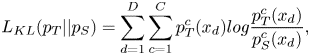
where $L_{KL}({p_{T}||p_{S}})$ represent the probability distribution of teacher and student model. We believe that the student model can get full of knowledge from teacher model by having distribution similar to teacher's distribution.
C) Offline ensemble
The original method of FSP [Reference Yim, Joo, Bae and Kim6] is discussed with one T-DNN to transfer one S-DNN. Compared with FSP [Reference Yim, Joo, Bae and Kim6], we propose using offline ensemble pre-trained teachers to generate the stochastic mean and improve the image classification result. The cost functions of knowledge distillation and KL Divergence are defined as
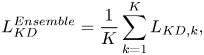

where $L_{KD}^{Ensemble}$ represents the loss function of offline ensemble knowledge distillation, $L_{KL}^{Ensemble}$
 represents the loss function of offline ensemble KL Divergence, $K$
 represents the numbers of pre-trained teacher models (K=3). We believe that the offline ensemble pre-trained teacher models with the same architecture, but the different weights will transfer knowledge to student model by using the stochastic mean.
D) Overall loss function
We had already proposed $L_{KD}$ , $L_{KL}$
 , and stochastic mean for our method. Hence, the overall loss function $L_{total}(\theta _{1})$
 for training S-DNN is shown as (9)
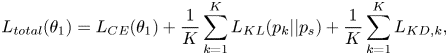
with the objective function of multi-class image classification $L_{CE}(\theta _{1})$ to train the network $\theta _{1}$
 is defined as the cross entropy error between the predicted values and the correct labels:

with an indicator function $I$ defined as
To prevent $L_{KD,k}$ larger than $L_{CE}(\theta _{1})$
 from inducing gradient explosion, we will adopt gradient clipping [Reference Pascanu, Mikolov and Bengio43] to limit the gradient of knowledge distillation$\nabla (\theta _{1})_{KD}^{clipped}$
 during training procedure as shown in Equation (12):


where $\beta$ is a sigmoid function. In Equation (13), $p$
 means the current epoch of training. Furthermore, the $L_{2}$
 -norm ratios are the $L_{CE}$
 and $L_{KD,k}$
 in Equation (14). Hence, the rich knowledge distilled from T-DNN can be transferred knowledge S-DNN without worrying about gradient explosion.
IV. EXPERIMENTAL RESULTS
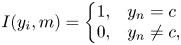
In this section, we will evaluate our proposed compression method with two datasets and three different models. The two datasets are the familiar CIFAR-100 [Reference Krizhevsky and Hinton44] and the rich collection of images, ImageNet64*64 [Reference Chrabaszcz, Loshchilov and Hutter45], as shown in Fig. 3. Additionally, there are two models, VGG and ResNet, training and testing on CIFAR-100 and one model named MobileNet, training and testing on ImageNet64*64.
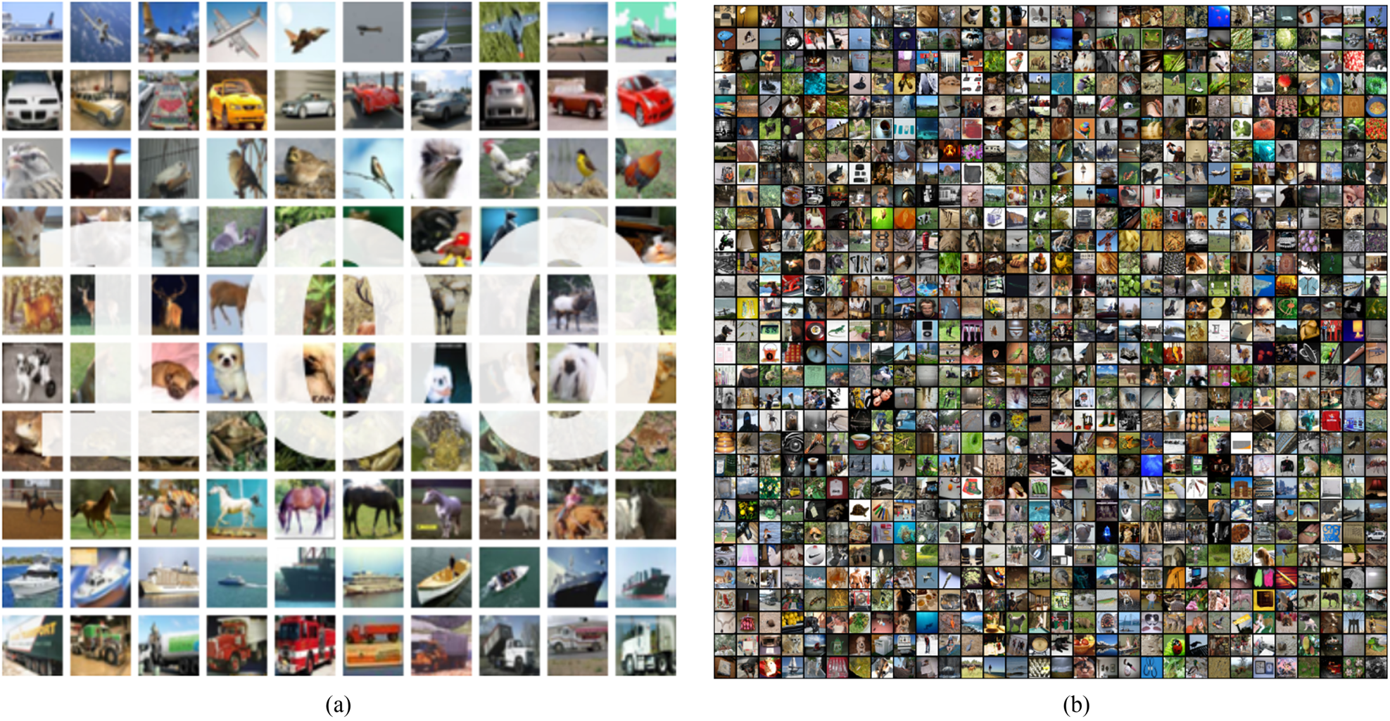
Fig. 3. (a) CIFAR-100. (b)ImageNet64*64.
A) Environment and datasets
Our proposed method is implemented in TensorFlow [Reference Abadi46] with Python 3.5 interference on the computers (CPU: Intel$^\circledR$ Core$^{TM}$
 i7-7800X $@$
 3.5 GHZ, main memory: 32 GB DRAM, GPU: NVIDIA GEFORCE $^\circledR$
 GTX 1080).
The CIFAR-100 dataset consists of 60000 images with a size of $32\times 32$ , divided as 50000 training data and 10000 test data, and 100 classes. We used random shift, random rotation and horizontal flip as data augmentations. Our proposed method was tested under the same conditions as FSP [Reference Yim, Joo, Bae and Kim6], and for increasing the dependability of the testing results, we ran the experiments three times and took the average as the final experimental results. We take VGG and ResNet as the DNN to prove that our proposed method works. The T-DNN and S-DNN models are shown in Fig. 4. We picked VGG as our first model because its architecture is very simple and can be implemented quickly. As in SSKD_SVD [Reference Lee, Kim and Song10], we defined VGG-11 as T-DNN and VGG-6 as S-DNN. As in FSP [Reference Yim, Joo, Bae and Kim6], we defined ResNet-32 as T-DNN and partially reduced the residual modules to create ResNet-8 as S-DNN.
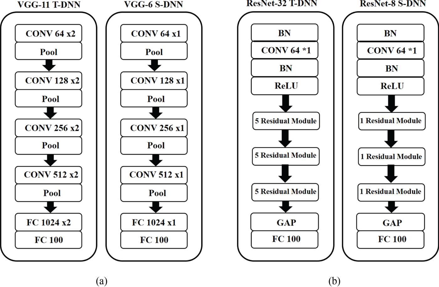
Fig. 4. T-DNN and S-DNN of the VGG and ResNet models. T-DNN: VGG-11 and ResNet-32. S-DNN: VGG-6 and ResNet-8.
The ImageNet64*64 dataset consists of about 1.2 million images with a size of 64$\times$ 64, divided with about 1.2 million training data and 50 000 test data, and 1000 classes. We used the same data augmentations as same with CIFAR-100 and the experiments were run three times and took the average as the final result. On ImageNet64*64, we defined MobileNet-16 as T-DNN and MobileNet-9 as S-DNN as shown in Fig. 5.
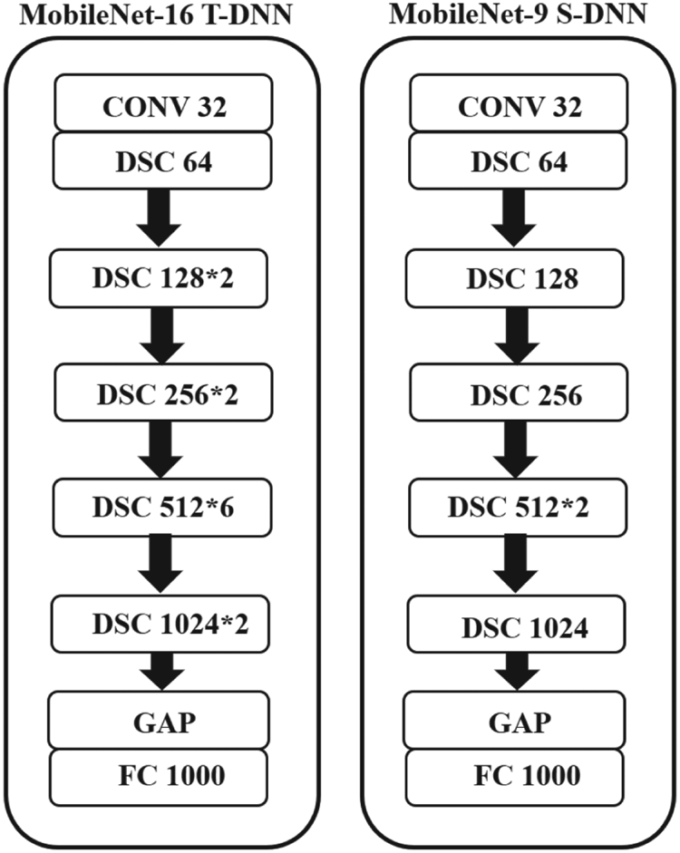
Fig. 5. T-DNN and S-DNN of the MobileNet models. T-DNN: MobileNet-16. S-DNN: MobileNet-9.
On CIFAR-100, the training procedure for networks was considered by FSP [Reference Yim, Joo, Bae and Kim6] and SSKD_SVD [Reference Lee, Kim and Song10]. We set the batch size to 128 and the training epochs to 200 during training, optimized the procedure by stochastic gradient descent [Reference Kiefer and Wolfowitz47], and adopted Nesterov accelerated gradient [Reference Nesterov48]. The initial learning rate was set to $10^{-2}$ and the momentum was set to 0.9. The decay parameter was set to $10^{-4}$
 . The learning rate was reduced to 0.1 per 50 epochs. Additionally, we set the batch size to 64 during training, training epochs to 40, and the learning rate was reduced to 0.1 per 10 epochs for ImageNet64*64.
B) Results
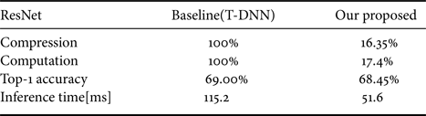
In this section, we show the final results of our proposed method with the computation rate, computation, Top-1 accuracy, and inference time. With VGG-11 as the teacher's model and VGG-6 as the student's model, experimental results show that the student's model increases 0.57% Top-1 accuracy while decreasing 53.9% of parameters and 72.8% computation compared to T-DNN and reducing inference time from 61.6 to 49.8 ms. Furthermore, with ResNet-32 as the teacher's model and ResNet-8 as the student's model, experimental results indicate that the student's model decreases 0.55% Top-1 accuracy by 0.55% while decreasing 83.65% of parameters and 82.6% computation compared to T-DNN and reducing inference time from 115.2 to 51.6 ms. The experimental results of VGG and ResNet are shown in Table 1 and 2, respectively. In most of the offline methods, the training procedure will lose some of their accuracies. However, it is surprising that our proposed method the S-DNN can train even better than T-DNN, as shown in Table 1.
Table 1. Classification results after knowledge distillation (VGG-11->6) on CIFAR-100 dataset.
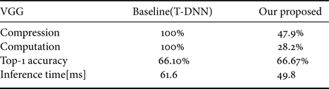
Table 2. Classification results after knowledge distillation (ResNet-32->8) on CIFAR-100 dataset.
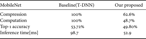
With MobileNet-16 as the teacher's model and MobileNet-9 as the student's model, experimental results show that the student's model decreases 3.92% Top-1 accuracy while decreasing 37.4% of parameters and 51.3% computation compare to T-DNN and reducing inference time from 98.7 ms to 52.9 ms. The results of MobileNet are shown in Table 3.
Table 3. Classification results after knowledge distillation (MobileNet-16->9) on ImageNet64*64.
C) Ablation
1) Cross-layer matrix
The different options of the cross matrix are shown in Fig. 6. Figure 6 (a) represents the “original” method FSP [Reference Yim, Joo, Bae and Kim6]. Figures 6(b) and 6(c) are our proposed methods in VGG and ResNet models. The combination of cross-one layer and cross-two layers is named as “P1(Cross two layers)”. Furthermore, the combination of cross-one layer, cross-two layers, and cross-three layers is named as “P1(Cross three layers)”.

Fig. 6. (a) Cross one layer. (b) Cross two layers. (c) Cross three layers.
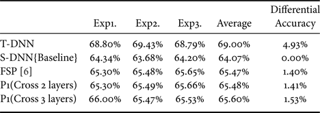
The simulation results of VGG models are shown in Table 4. The result of S-DNN is set as the baseline. Compared with the baseline, the method of “P1(Cross two layers)” and “P1 (Cross three layers)” achieves a low performance in the testing result. Additionally, “P1 (Cross three layers)” have an increase in performance of 0.4% compared with FSP [Reference Yim, Joo, Bae and Kim6]. Subsequently, let us see the deeper architecture ResNet as shown in Table 5. Moreover, the methods of “P1(Cross two layers)” and “P1 (Cross three layers)” achieve a low performance in the testing results. The “P1 (Cross three layers)” have an increase in performance of 0.13% compared with FSP [Reference Yim, Joo, Bae and Kim6].
Table 4. Different proposed method of cross matrix (VGG-11->6) with CIFAR-100. T-DNN: VGG-11, S-DNN: VGG-6.
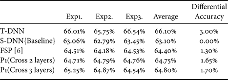
Table 5. Different proposed method of cross matrix (ResNet-32->8) with CIFAR-100. T-DNN: ResNet-32, S-DNN: ResNet-8.
Additionally, the different choices of the cross-layer matrix are shown in Fig. 7. Figure 7 (a) represents the ‘original’ method FSP [Reference Yim, Joo, Bae and Kim6]. Figures 7(b)–7(d) are our proposed methods with MobileNet model. The combination of cross-one layer and cross-two layers are named as “P1(Cross two layers)”. Additionally, the combination of cross-one layer, cross-two layers, and cross-three layers is termed as “P1(Cross three layers)”. Finally, the combination of cross-one layer, cross-two layers, cross-three layers, and cross-four layers is named as “P1(Cross four layers)” .

Fig. 7. (a) Cross-one layer. (b) Cross-two layers.(c) Cross-three layers. (d)Cross-four layers.
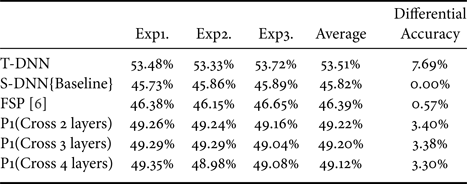
The results of MobileNet model are shown in Table 6. Compared with the baseline, the methods of ’‘P1(Cross two layers)” and ‘’P1 (Cross three layers)” achieve a low performance in the testing result. Furthermore, “P1 (Cross three layers)” has increased performance of 3.38% compared with FSP [Reference Yim, Joo, Bae and Kim6].
Table 6. Different proposed method of cross matrix (MobileNet-16>9) with ImageNet64*64. T-DNN: MobileNet-16, S-DNN: MobileNet-9.
2) Influence of adding KL Divergence
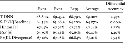
The illustration of adding KL Divergence as our second-order loss function is shown in Fig. 8. We believe that the student's model can get full of knowledge from the teacher's model by being similar to the teacher's distribution. The combination of FSP [Reference Yim, Joo, Bae and Kim6] and adding KL Divergence is named as “P2 (KL Divergence)”. First, let us see the result of VGG models as shown in Table 7. Additionally, the result of S-DNN is set as the baseline. We have two competitors. The first is the proposed Hinton [Reference Hinton, Vinyals and Dean7] approach and our basis FSP [Reference Yim, Joo, Bae and Kim6]. It is demonstrated that adding KL Divergence yields a 1.54% increase over the competitor FSP [Reference Yim, Joo, Bae and Kim6]. Furthermore, the experimental results of ResNet are shown in Table 8. It indicates that adding KL Divergence yields a 1.54% increase over the competitor FSP [Reference Yim, Joo, Bae and Kim6].
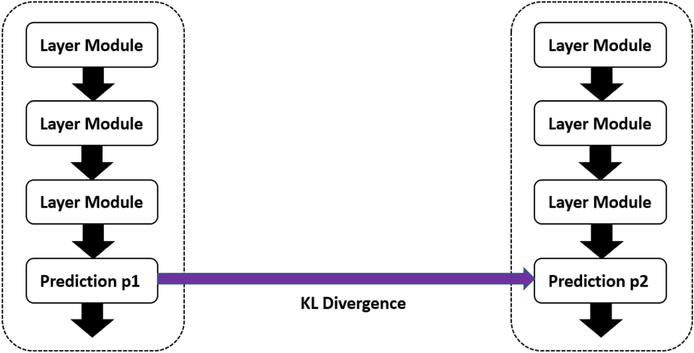
Fig. 8. Illustration of using KL Divergence.
Table 7. Differential of adding KL Divergence (VGG-11>9) with CIFAR-100. T-DNN: VGG-11, S-DNN: VGG-6.
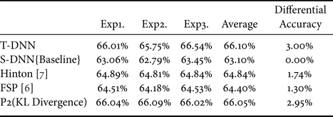
Table 8. Differential of adding KL Divergence (ResNet-32->8) with CIFAR-100. T-DNN: ResNet-32, S-DNN: ResNet-8.
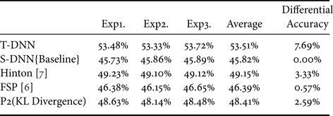
On ImageNet64*64, the experimental results of MobileNet models are shown in Table 9. We have two competitors, the first is the proposed Hinton [Reference Hinton, Vinyals and Dean7] approach and our basis FSP [Reference Yim, Joo, Bae and Kim6]. It is shown that adding KL Divergence that obtains a 2.59% increase over the competitor FSP [Reference Yim, Joo, Bae and Kim6].
Table 9. Differential of adding KL Divergence (MobileNet-16>9) with ImageNet64*64. T-DNN: MobileNet-16, S-DNN: MobileNet-9.
3) Offline ensemble
In this section, we will discuss the influence of the number of multiple pre-trained teachers as shown in Fig. 9. Figure 9(a) uses one pre-trained teacher as FSP [Reference Yim, Joo, Bae and Kim6]. Figures 9(b) and 9(c) represent two pre-trained teachers and three pre-trained teachers named as “P3 (two teachers)” and “P3(three teachers)”, respectively. First, let us see the result of VGG model in Table 10. Additionally, the result of S-DNN is set as the baseline. From Table 10, we find that using more pre-trained teachers with stochastic mean can increase the Top-1 accuracy. It is shown that offline ensemble yields a 1.66% increase over the competitor FSP [Reference Yim, Joo, Bae and Kim6]. In addition, let us see the deeper model ResNet. From Table 11, we can also find that using more teachers can increase the Top-1 accuracy. It is demonstrated that offline ensemble obtains a 1.31% increase over the competitor FSP [Reference Yim, Joo, Bae and Kim6]. Finally, let us see the result of MobileNet models as shown in Table 12. It is demonstrated that adding KL Divergence yields a 2.59% increase over the competitor FSP [Reference Yim, Joo, Bae and Kim6].
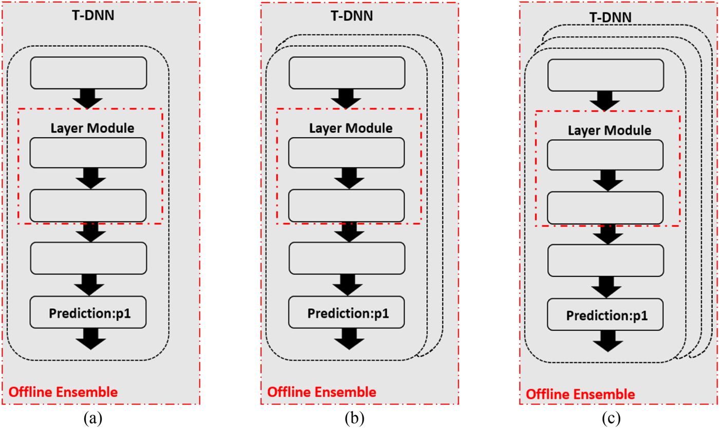
Fig. 9. (a) One pre-trained teacher. (b) Two pre-trained teachers. (c) Three pre-trained teachers.
Table 10. Different numbers of teachers (VGG-11->6) with CIFAR-100. T-DNN: VGG-11, S-DNN: VGG-6.

Table 11. Different numbers of teachers (ResNet-32->8) with CIFAR-100. T-DNN: ResNet-32, S-DNN: ResNet-8.

Table 12. Different numbers of teachers (MobileNet-16->9) with ImageNet64*64. T-DNN: MobileNet-16, S-DNN: MobileNet-9.

4) Combination of proposed methods
By analyzing prior work, we want to try a combination of proposed methods. The combination of crossing one layer, adding KL Divergence and offline ensemble is shown in Tables 13 and 14.
Table 13. Combination of proposed methods (VGG-11->6) with CIFAR-100. T-DNN: VGG-11, S-DNN: VGG-6. P1: cross-three layers. P2: KL Divergence. P3: three pre-trained teachers.
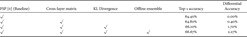
Table 14. Different proposed method of cross matrix (ResNet-32->8) with CIFAR-100. T-DNN: ResNet-32, S-DNN: ResNet-8. P1: cross-three layers. P2: KL Divergence. P3: three pre-trained teachers.

First, let us see the result of VGG with the combination of crossing three layers, adding KL Divergence and offline ensemble. From Table 13, we can see that by adding the proposed method increases the Top-1 accuracy. It is shown that the combination of proposed method gets an increase of 2.27% than FSP [Reference Yim, Joo, Bae and Kim6]. Second, let us see the deeper ResNet model with the combination of proposed methods. From Table 14, we can see that by adding the proposed method to increase the Top-1 accuracy. It is shown that the combination of proposed method gets an increase of 2.98% than FSP [Reference Yim, Joo, Bae and Kim6]. Finally, from Table 15 we can see that by adding proposed method to increase the Top-1 accuracy, the combination of proposed method get 4.04% increase than FSP [Reference Yim, Joo, Bae and Kim6].
Table 15. Combination of proposed methods (MobileNet) with ImageNet64*64. T-DNN: MobileNet-16, S-DNN: MobileNet-9. P1: cross-three layers. P2: KL Divergence. P3: three pre-trained teachers.

D) Comparison with other work
With the same compression on S-DNN, it can be seen that our proposed method got the state-of-the-art results on VGG and ResNet models compared with the competitors [Reference Yim, Joo, Bae and Kim6, Reference Hinton, Vinyals and Dean7, Reference Lee, Kim and Song10, Reference Park, Kim, Lu and Cho11]. As we can see in Table 16, the result of our proposed method achieves a 66.67% Top-1 accuracy with a 2.08x compression rate and 3.5x computation rate. Additionally, the result of our proposed method achieves a 68.45% Top-1 accuracy with a 6.11x compression rate and 5.27x computation rate as shown in Table 17. Furthermore, we can see in Table 18 that the result of our proposed method achieves a 49.86% Top-1 accuracy with a 1.59x compression rate and 2.05x computation rate.
Table 16. Computation, parameters, and average Top-1 accuracy comparison with VGG-11 and VGG-6 on CIFAR-100. T-DNN: VGG-11, S-DNN: VGG-6.

Table 17. Computation, parameters, and average Top-1 accuracy comparison with ResNet-32 and ResNet-8 on CIFAR-100. T-DNN: ResNet-32, S-DNN: ResNet-8.

Table 18. Computation, parameters, and average Top-1 accuracy comparison with ResNet-32 and ResNet-8 on CIFAR-100. T-DNN: ResNet-32, S-DNN: ResNet-8.

V. DISCUSSION
In this section, we show what our proposed methods meet limitations. After that, we will compare solutions with the previous proposed methods and discuss why some of our proposed new ideas make our S-DNN get better performance with the same compression.
A) Constraints of our proposed method
FSP [Reference Yim, Joo, Bae and Kim6] proposed a certain layer group in the network and defined the correlation between input and output feature maps of the layer group as Gramian matrix. The limitation is that the T-DNN and S-DNN should have the same channels, as shown in Fig. 10. If the Gramian matrices of T-DNN and S-DNN do not have the same dimension, $m_{T}=m_{s}$ and $n_{T}=n_{S}$
 , then they cannot be calculated as loss function. Furthermore, we find that huge difference layers between T-DNN and S-DNN may cause the difficulty in transferring knowledge, as shown in Fig. 11. Hence, we define “the T-DNN and S-DNN should have the same channels” and “the huge difference layers between T-DNN and S-DNN” as constraint 1 and constraint 2, respectively.

Fig. 10. Limitation of FSP [Reference Yim, Joo, Bae and Kim6]. $m_{T},\,n_{T}$ represent the dimension of T-DNN Gramian matrix and $m_{S},\,n_{S}$
 represent the dimension of S-DNN Gramian matrix.

Fig. 11. Illustration of huge layer number difference. C, convolutional layer; FC, fully-connected layer.
B) Solutions
How to make the Gramian matrices of T-DNN and S-DNN with same dimension is the key to solving constraint 1. As a result, we propose to use 1x1 convolution layers to forcibly tune output channels of T-DNN. In Fig. 12, the color in orange layers are the additional convolutional $1\times 1$ layers. Because the additional convolutional layer only works in the training procedure, the parameters of T-DNN and S-DNN are the same with the original ones. Moreover, we propose two-step compression to solve constraint 2 as shown in Fig. 13. We believe that using “Teacher” T-DNN to teach a temporary neural network model “Temporal”, then use the “Temporal” to teach the final target neural network model “Student”.

Fig. 12. Using $1\times 1$ convolutional layers to decrease channels.

Fig. 13. The illustration of two-stage knowledge distillation. C, convolutional layer; FC, fully connected layer.
Based on our proposed method, we do not have the experiments on greatly reducing the depth of the student model. There are two reasons. First, if we greatly reduce the depth of the student model, the image sizes after passing the student module with reduced depth are different from that of the original student model, the issue of how to align with the teacher model needs to be resolved. Second, to remove the number of Res-blocks to three in some Res-blocks could make the top-1 accuracy drop heavily since the CNN model may not learn enough details from the feature maps.
As a result, we do not change the structure of ResNet. We decrease the student model to the lowest number of the ResNet layers to create the smallest size and computation of the ResNet-10 as shown in Fig. 14.
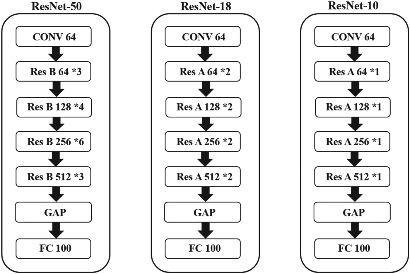
Fig. 14. ResNet-50/ResNet-18 /ResNet-10.
C) Experiments and results
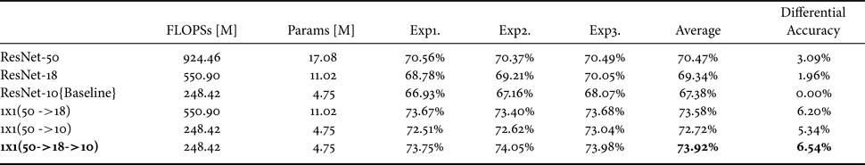
Using the same environment details of CIFAR-100 datasets, we set the batch size to 64 during training and training epochs to 200. We use ResNet-50 as the teacher's model and ResNet-10 as the student's model and ResNet-18 as the temporal model, as shown in Fig. 14. Experimental results show that the student's model increases the Top-1 accuracy by 3.45% and decreases 72.19% of parameters and 73.16% computation compared to T-DNN and reduces inference time from 188.9 ms to 66.3 ms. The experimental results of ResNet are shown in Table 19. Compared with ResNet-10 in Table 20, by using $1\times 1$ convolutional layers and our proposed method, ResNet-18 can obtain a 6.20% differential accuracy. Furthermore, by using two-stage KD, we could increase the differential accuracy by a further 6.54%. We believe that using two-stage knowledge distillation can prevent the loss of KD.
Table 19. Classification results after knowledge distillation (ResNet-50->10) with CIFAR-100 dataset.

Table 20. Methods of adding $1\times 1$ convolution to solve the limitation of proposed method and multi-steps compression with ResNet models and CIFAR-100. T-DNN1: ResNet-50. T-DNN2: ResNet-18. S-DNN: ResNet-10.
VI. CONCLUSION
In this paper, we propose a method using cross-layer knowledge distillation with KL divergence and offline ensemble to extract more knowledge from T-DNN to S-DNN to improve the Top-1 accuracy of image classification. Moreover, we use a $1\times 1$ convolutional layer to tune the dimension of Gramian matrix to solve the limitation of our proposed method and we further propose a method, two-stage KD, to avoid the loss of knowledge transfer.
Hsin-Hung Chou received a B.S. degree in Communications, Navigation and Control Engineering from National Taiwan Ocean University, Taipei, Taiwan. He received M.S. degree in the Department of Communications Engineering, National Tsing Hua University, Hsinchu, Taiwan. His research topics focused on Deep Neural Network models compression with heuristic methods. He is now working in Cisco Taiwan and is a consulting engineer. He is focusing on 5G Core Network and importing 5GCN in manufacturing industries with automation tools to help customers digital transformation.
Ching-Te Chiu received her B.S. and M.S. degrees from National Taiwan University, Taipei, Taiwan. She received her Ph.D. degree from University of Maryland, College Park, Maryland, USA, all in electrical engineering. She is a Professor at the Computer Science Department and Institute of Communications Engineering, National Tsing Hua University, Hsinchu, Taiwan. Currently, she is the Director of Institute of Information Systems and Applications, National Tsing Hua University, Hsinchu, Taiwan. She was member of technical staff with AT&T, Lucent Technologies, Murry Hill, NJ, USA, and with Agere Systems, Murry Hill, NJ, USA. Her research interests include Machine Learning, Pattern Recognition, High Dynamic Range Image and Video Processing, Super Resolution, High Speed SerDes design, Multi-chip Interconnect, and Fault Tolerance for Network-on-Chip design. Dr. Chiu won the first prize award, the best advisor award, and the best innovation award of the Golden Silicon Award. She served as the Chair of IEEE Signal Processing Society, Design and Implementation of Signal Processing Systems (DISPS) TC. She is a TC member of the IEEE Circuits and Systems Society, Nanoelectronics and Gigascale Systems Group. She was the program chair of the first IEEE Signal Processing Society Summer School at Hsinchu, Taiwan 2011 and technical program chair of IEEE workshop on signal processing system (SiPS) 2013. She served as associate editor of IEEE Transactions on Circuits and Systems I and served as associate editor of IEEE Signal Processing Magazine and Journal of Signal Processing Systems.
Ms. Yi-Ping Liao Student at University of National Tsing Hua.


 Open access