

I. INTRODUCTION
End-to-end delay is an important concern for two-way visual communication applications. Video codec manufacturers need to measure the end-to-end delay of a video codec system in order to develop low-delay video codecs. Network service providers need to make sure the end-to-end delay of a visual communication application is within the application requirement. A simple and general tool for measuring the end-to-end delay of a visual communication system is invaluable for applications related to two-way visual communications.
Figure 1 shows an example of a mobile video chat system. Video captured by the camera is compressed by a video encoder. The encoder usually contains an encoder buffer to smooth the video bit-rate as described in [Reference Reibman and Haskell1]. The video bit-stream is then packetized and transmitted over the network. At the decoder side, the video is decoded and displayed. The decoder usually contains a decoder buffer to smooth out the network jitter and to buffer the bit-stream before the video decoding. The encoder and decoder buffers can result in a relatively long delay. The end-to-end delay in this example, is the latency from frame capturing at the encoder side to the frame display at the decoder side, which we call capture-to-display delay (CDD), including the whole chain of video encoding, encoder buffering, packetization, network transmission, decoder buffering, and video decoding.

Fig. 1. An end-to-end visual communication system.
The traditional way to measure the latency is by using timestamps. A timestamp is a code representing the global time. It can be generated by a counter driven by a network clock commonly available to both the encoder and the decoder. To measure the time delay between two points A and B, a timestamp is inserted at point A, retrieved at the point B, and compared with the global time at point B. For example, for the visual communication system shown in Fig. 1, to measure the end-to-end delay of the network part, timestamps are generated from the network clock and inserted at the network interface point in the encoder side. These timestamps are retrieved at the network interface point at the decoder side to compare with the global time. Similarly, to measure the CDD, we can insert timestamps at the video capture point, and observe the timestamps relative to the global time at the display point. As long as a network clock is available and the encoder clock and the decoder clock are synchronized, the delay can be calculated. However, in order to do this, we need to be able to modify the hardware or software to insert the timestamps, and retrieve the timestamps at the desired points. In many situations including our application scenario, cellphone video codecs are implemented in hardware and software by the developers. Thus, we cannot modify the video encoder and decoder to insert or retrieve the timestamps. Also, usually the encoder clock and the decoder clock are not synchronized. These make the measuring of the CDD particularly challenging.
Boyaci et al. [Reference Boyaci, Forte, Baset and Schulzrinne2] presented a tool to measure the CDD of a video chat application running on a personal computer (PC) platform. Their approach adds timestamps represented in barcodes at the encoder side. After the video is decoded at the decoder side, the barcodes are recognized and compared with the time at the decoder side. However, this method still requires the development of new software inside the encoder and decoder machines in order to insert and recognize the barcodes and compare the recognized timestamps with the system time. Moreover, the encoder clock and the decoder clock need to be synchronized. Kryczka et al. [Reference Kryczka, Arefin and Nahrstedt3] extended the tool “vDelay” [Reference Boyaci, Forte, Baset and Schulzrinne2] and added tools to measure mouth-to-ear latency and the audio–visual synchronization skew. The tool is called “AvCloak”. Since [Reference Kryczka, Arefin and Nahrstedt3] is built on top of [Reference Boyaci, Forte, Baset and Schulzrinne2], it also requires installation of new software and clock synchronization between encoder and decoder. Some other works to measure the delay of video chat applications over two computers are in [Reference Jansen and Bulterman4,Reference Xu, Yu, Li and Liu5].
As an increasing number of people have video chats via cellphones, the measurement of CDD with cellphone is important. Previous solutions (e.g. vDelay and AvCloak) for PCs are not suitable for cellphones, since it is difficult to synchronize the clocks on the cellphones and access to the video encoding and decoding systems inside the cellphones In addition, to recognize the timestamps, those software require access to the screen on the receiver's side. However, the hardware or software cannot be modified to achieve that in the cellphone chatting scenarios. In this work, we address the technical problem “how to measure the CDD associated with a practical video chat application between two cellphones in a research environment?” We would like to emphasize that, different from the existing measurement methods for video chatting on two PCs, the main constraint in this problem is that, we cannot modify the video chat applications and synchronize the clock in these two cellphones.
To overcome the aforementioned problems, we propose a method that can be used to measure the CDD of any visual communication applications, which does not require modification to the application source code and access to the inside of the system. It also does not require the encoder and decoder clocks to be synchronized. It is based on the simultaneous recognitions and comparisons of visual patterns of both timestamps captured at the encoder side and displayed at the decoder side. Our contributions include: (1) a proposal on a new CDD measurement method that does not require modification to the visual communication system nor synchronization between the encoder and decoder clocks; (2) a solution to the multiple-overlapped-timestamp problem encountered using this approach; and (3) a measurement error analysis for this approach.
The organization of the rest of this paper is as follows. In Section II, we discuss our approach of measuring the CDD. In Section III, we discuss the problem of multiple-overlapped timestamps. In Section IV, we present our solution to the overlapped timestamps problem. In Section V, we present experimental results to show the effectiveness of our proposed methods. Section VI concludes the paper.
II. PROPOSED METHOD FOR DELAY MEASUREMENT
A) The proposed CDD measurement approach
The proposed CDD measurement approach is shown in Fig. 2. Timestamps representing a stopwatch with millisecond precision are displayed on the screen of an external PC, Cellphone1, and Cellphone2 establish the video chat connection. The timestamps shown on the screen of the PC are captured by the Cellphone1 camera. In order to make the measurement close to a realistic scenario, we pre-record a chat-like video sequence and play it behind the timestamp, so that the video contains both timestamp and the chatting person. The video of Cellphone1 is encoded and transmitted to Cellphone2. The decoded video is displayed on the screen of Cellphone2. A webcam records the timestamps on both the screens of the PC and Cellphone2. The delay measurement software in the PC receives the video from the webcam, and performs pattern recognitions for the two timestamp patterns in the video frame. The value of the difference between the two timestamps is the CDD. Note that the CDD measurement is usually performed in research for investigating the end-to-end delay. In this application scenario, the network provider or the codec manufacturer has the control on routing the packets or using a network simulator to simulate the network. So the sender/receiver/PC have to be at the same site is not a serious limitation of the proposed approach. This work actually comes out from a real-life situation. In this actual situation, we like to know how much delay is due to the video codec in a video chat application over cellphones. However, since the video codec is embedded in the cellphone, a way to be able to measure the video codec delay is needed. Our proposed method addresses this need. There are many other situations with the similar need such as a video codec vendor who like to measure the delay of their video codecs, or low delay coding researchers who like to know the end-to-end delay of their approaches. In all these kinds of applications, the encoder and decoder at the same location is not a problem at all.
Fig. 2. The proposed approach to measure the CDD. The difference between timestamps on the computer's screen and Cellphone2’s screen is the CDD.
The software is implemented in an external PC which includes two applications: CDD-T (for transmitter) and CDD-R (for receiver). The CDD-T application generates and displays timestamps on the PC screens every T stamp time. The CDD-R application receives the captured video from the webcam, performs timestamp pattern recognitions, and calculates and displays the CDD of every frame. At the end of a measurement session, the CDD-R application will also output the delay statistics such as the minimum, maximum, mean, and the standard deviation of CDD.
B) Timestamp representations
The timestamps can be represented in different patterns. Two example patterns we investigated to encode the timestamps are shown in Fig. 3. Figure 3(a) represents a timestamp in digits and Fig. 3(b) represents a timestamp in a quick response (QR)-code [Reference Ohbuchi, Hanaizumi and Hock6]. There is public domain software that can recognize the digit and QR-code timestamps. The digital timestamps can be read by the user to get a quick read of the CDD. The QR-code is not human-readable. However, the fast readability and greater storage capacity compared with the standard barcodes make the QR-code increasingly popular. For error-resiliency, Boyaci et al. [Reference Boyaci, Forte, Baset and Schulzrinne2] used an european article number (EAN)-8 barcode because of its checksum mechanism. The EAN-8 barcode with a checksum can allow to detect whether the timestamp is contaminated, and refuse to read the barcode if it is damaged or distorted. The QR-code not only has the checksum mechanism but also the error correction capability. Even if a QR-code has some local breakage, it still can restore the original information. Furthermore, the QR-code is designed with open standards.
Fig. 3. Examples of timestamp formats (a) digits and (b) QR-code.
III. PROBLEM OF MULTIPLE-OVERLAPPED TIMESTAMPS
Although the concept of the above proposed approach looks simple, during our experiments, we found it has a problem of multiple-overlapped timestamps due to the limited camera shutter speed. In this section, we study this problem and show the relationship between the maximum number of overlapped timestamps and the camera exposure time.
A) Problems of multiple-overlapped timestamps
When we use a camera to capture the timestamps, the camera needs some time to expose a frame. The exposure process is related to the camera's aperture and shutter speed [Reference Ray, Axford, Attridge and Jacobson7], with the exposure time T e, which is the duration of time when the camera shutter is open. Timestamps refresh quickly so that different timestamps appear during the exposure period, and all these timestamps are captured by the image sensor. This results in multiple-overlapped timestamps on the display as shown in Fig. 4. Using public domain software to recognize the multiple overlapped-timestamp patterns causes serious errors. We cannot just discard the blurred timestamp frames, because only about 50% of the frames are clear in our experiments. Here, a clear frame means that the timestamps on both the PC and the Cellphone2 screens could be correctly recognized. It is also observed that the most recent timestamp may not be the most visible timestamp in the multiple-overlapped timestamps.
Fig. 4. Multiple overlapped-timestamps: (a) with digits and (b) with QR code.
B) Relationship between the maximum number of overlapped timestamps and the camera exposure time
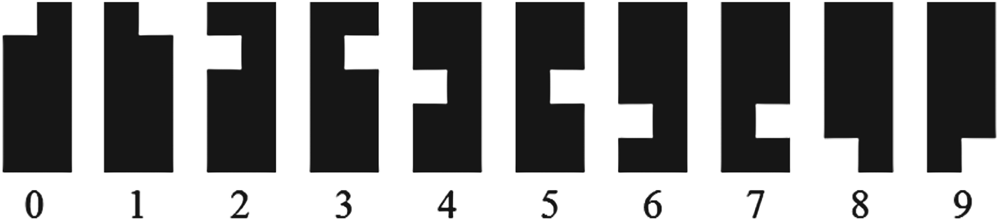
To investigate the extent of the multiple-overlapped timestamps and confirm the reason of multiple-overlapped timestamps, we design a set of visual patterns to represent the 10 digits as shown in Fig. 5. A black rectangular pattern is split into 5 × 2 sub-blocks and the position of the white sub-block represents a digit so that this visual pattern is still human-readable. Since the white squares in the patterns appear at different locations for different digits, we can easily see how many timestamps are overlapped by counting the numbers of brighter squares in the area representing a digit. One example is shown in Fig. 6.
Fig. 5. Special visual patterns and corresponding digits.
Fig. 6. Multiple overlapped-timestamps with special visual patterns. The number of overlapped patterns can be easily counted.
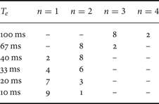
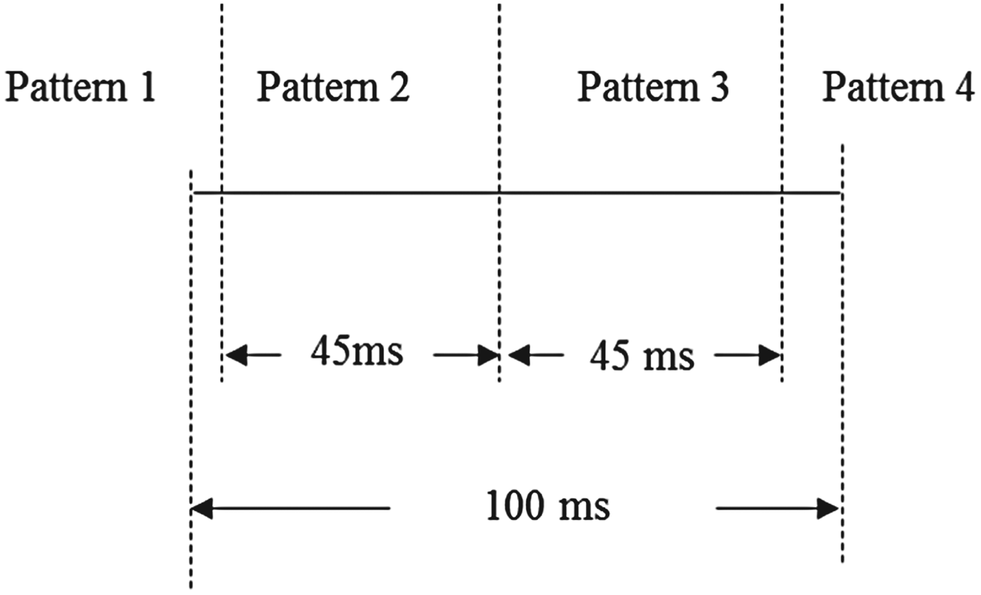
With these visual patterns, we conduct an experiment as follows: fix the timestamp refresh interval and change the camera exposure time. We fix T stamp to 45 ms and set the webcam exposure time T e to 100, 67, 40, 33, 20, and 10 ms in each test, take 10 pictures of timestamps on the PC screen, and count the number of overlapped timestamps, denoted as n, in these pictures. The result is shown in Table 1.
Table 1. Statistics of pictures with different number of overlapped patterns.
Results in Table 1 follow an equation:
 $$N = \lfloor{T_e /T_{stamp}} \rfloor +2\comma \; $$
where ⌊ • ⌋ is the floor function and N is the maximum number of overlapped patterns on PC given the exposure time and the timestamp refresh interval. Equation (1) can be explained with an example in Fig. 7, with T e = 100 ms and T stamp = 45 ms. Under this situation, in the worst case, there are two extra timestamps partially appearing at the beginning and the end of the exposure period, so that the overlapped patterns contain two fully exposed timestamps and two partially exposed timestamps.
Fig. 7. Example of the worst case when the maximum number of overlapped timestamp occurs.
Note that equation (1) works for one exposure, however, in our measurement system, the timestamps on Cellphone2 are exposed twice: the first is the exposure via Cellphone1 and the second is the exposure via the webcam facing PC and Cellphone2. In this scenario, the maximum number N′ of overlapped timestamps on Cellphone2 could be
 $${N}^{\prime}=N_1 \times N_2\comma \; $$
where N 1 is the maximum number of overlapped timestamps derived by equation (1) in the first exposure, and N 2 is the maximum number of overlapped timestamps due to the exposure time of the webcam, which can be determined similar to equation (1) by:
 $$N_2 =\lfloor{T_e /T_{c1\_camera}} \rfloor +2\comma \; $$
where T e is the expose time of the webcam and T c1_camera is the display frame time of the Cellphone2 which is determined by the video encoding frame rate of camera of the Cellphone1.
From the above experiments, we can conclude that the longer camera exposure time causes the overlapped timestamp problem and more overlapping problems appear on Cellphone2 than on PC according to equation (2). A shorter timestamp refresh interval and/or a longer camera exposure time will make the overlapped timestamp problem worse. To overcome the overlapped timestamp problem, one straightforward method is to minimize T e. However, in our measurement system, the exposure time of the built-in camera of Cellphone1 cannot be set manually. Another method is to maximize the timestamp refresh interval time. However, a long refresh interval increases the measurement error, which will be discussed further in Section IV.
IV. SOLUTION OF OVERLAPPED TIMESTAMPS – SPACE DIVERSITY AND COLOR DIVERSITY
From equations (1) and (2) we can see that the overlapping timestamp problem is inevitable (N ≥ 2 in equation (1)) on both PC and Cellphone2 screens. Decreasing the camera exposure time or increasing timestamp refresh interval can only reduce the possibility of occurrence of the multiple-overlapped-timestamp problem, rather than solve it completely. In this section, we propose a solution to the overlapped timestamp problem.
A) Use space diversity to solve the multiple-overlapped-timestamp problem
We solve the problem with space diversity, i.e. displaying consecutive timestamps at different locations so that they do not overlap before they disappear. The number of space diversity D s depends on the maximum possible number of overlapped timestamps. A video frame showing the QR-codes with a space diversity of four is shown in Fig. 8.
Fig. 8. A video frame showing the QR-codes with a space diversity of four.
B) Combining color diversity to handle more overlapped timestamps and reduce timestamp area
Using space diversity can separate timestamps successfully, but to handle more overlapped patterns, increasing the number of the space diversity may look awkward in the practical use. In this case, we can combine the color diversity to handle more overlapped timestamps.
The main idea is to allow multiple timestamps captured by the camera but make them separable in the color space. Based on this, the visual patterns we designed in Fig. 5 can add a color attribute (red, green, and blue); the example of digit 0 is shown in Fig. 9(a). Using color diversity, we can solve the problem when timestamps with different color are overlapped. One example is shown in Fig. 9(b). In this example, one green and one blue timestamp are overlapped. By extracting the green and blue components separately, we can segment the two timestamps.
Fig. 9. (a) Visual pattern for digit 0 with different colors and (b) an example of two-overlapped timestamps, which are separable in the color space. Green timestamps represent “03771” and blue timestamps represent “03765”. (Best viewed in color.)
Combining D s number of space diversity and D c number of color diversity can handle up to D s × D c number of overlapped timestamps. So in our simulation test, to handle four overlapped timestamps, we can use two space diversity combined with three color diversity. In this way, we save two spaces for timestamps compared with using only the space diversity method. Theoretically, we could extend to more colors to increase the color diversity. However, it will make the detection of different colors under multiple-overlapped timestamps more difficult. In Section V, we test both the space diversity method and the space + color diversity method.
C) Measurement error analysis
Using the above space and color diversity methods, the timestamps can be recognized accurately (the recognition accuracy can reach 99.4%, as will be shown in Section V). However, due to the limited time resolutions of the timestamp generating, PC screen refreshing, Cellphone1 capturing, and Cellphone2 displaying the actual time may not be identical to the timestamp time, so measurement errors are induced into the measured delay. In this part, we analyze the measurement error.
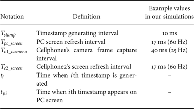
To make the analysis easier to understand, we define some notations in Table 2.
Table 2. Notations related to the measurement error analysis.
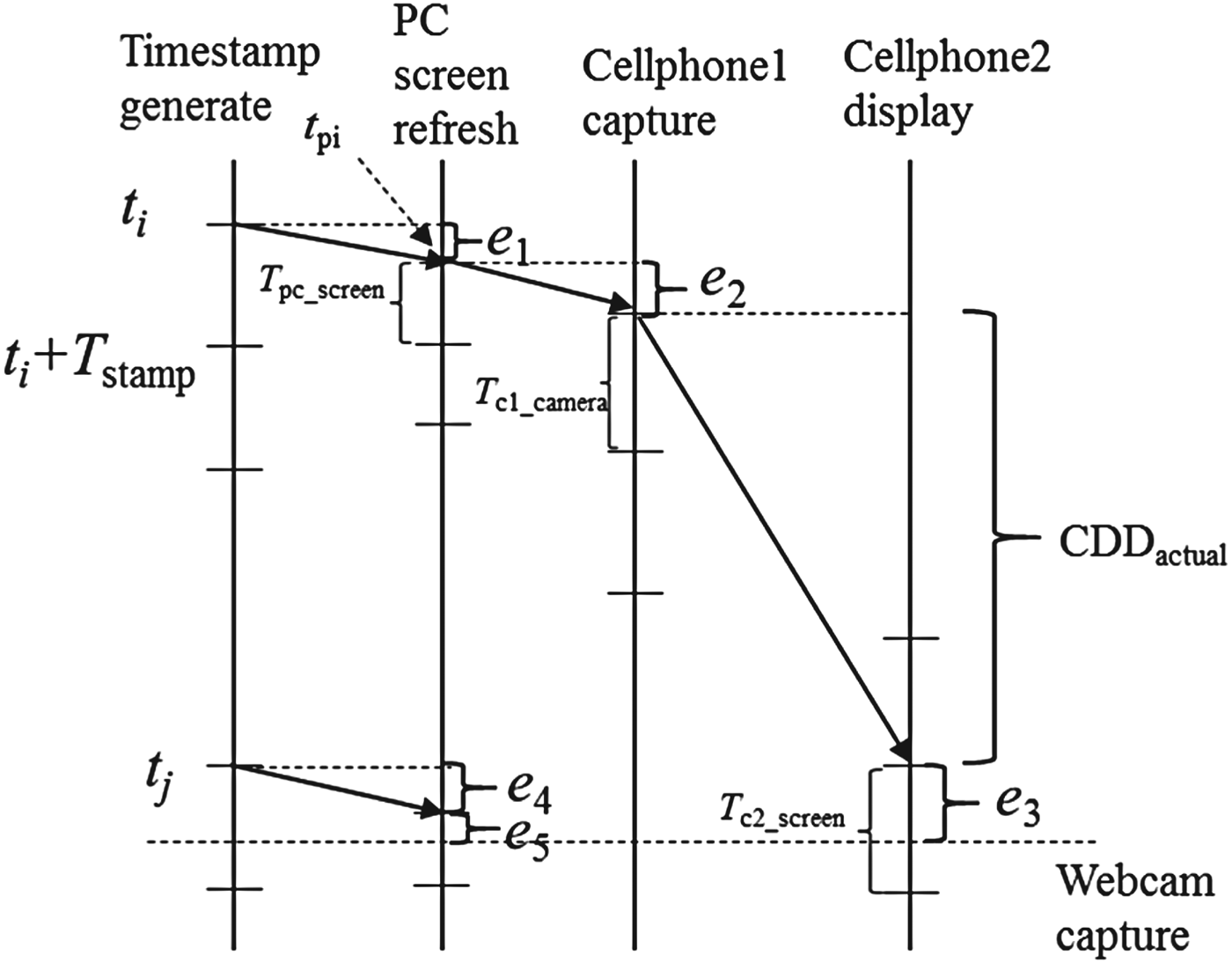
Without losing generality, the measure process can be described in a timeline shown in Fig. 10.
Fig. 10. Timeline of timestamps on different devices. The bottom dashed line indicates the time when timestamps on PC screen and Cellphone2 screen are captured by the webcam.
The displaying and capturing can be modeled as sampling processes. We discuss steps in details as follows:
(1) Timestamp is generated in the PC every T stamp time.
(2) PC screen samples the timestamp sequence and display the timestamps on the screen every T pc_screen time.
(3) Cellphone1 captures the PC screen every T c1_camera time.
(4) Cellphone2 receives and decodes the frame from Cellphone1, then displays the frame sequence every T c2_screen time.
(5) Webcam captures (a) PC's screen and (b) Cellphone2's screen.
Among the above steps, (2), (3), (4), and (5) can be modeled as sampling processes, which induce measurement errors shown in Fig. 10. For example, in step (2), the time when PC screen refreshes is t pi, which is
 $$t_{i} \le t_{pi} \lt t_i +T_{stamp}. $$
The difference between the displaying time t pi and the actual time t i is
 $$e_1 =t_{pi} -t_{i}. $$
Since the timestamp generating and PC screen refreshing processes are independent, this e 1 follows a uniform distribution,
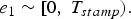 $$e_1 \sim \lsqb {0\comma \; T_{stamp}} \rpar .$$
Note that e 4 associated with the timestamp t j in Fig. 10 has the same distribution of e 1, since it comes from the same process as step (2).
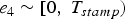 $$e_4 \sim \lsqb 0\comma \; T_{stamp}\rpar $$
Similarly, based on this sampling model, e 2, e 3, and e 5 are errors involved in step (3), (5a), and (5b), and they all follow the uniform distribution:
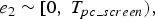 $$e_2 \sim \lsqb {0\comma \; T_{pc\_screen}} \rpar \comma \; $$
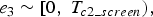 $$e_3 \sim \lsqb {0\comma \; T_{c2\_screen}} \rpar \comma \; $$
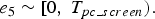 $$e_5 \sim \lsqb {0\comma \; T_{pc\_screen}} \rpar . $$
The CDD is defined as the time from Cellphone1 captures the PC's screen to Cellphone2 displays that frame, which is denoted as CDD actual. However, the measured delay CDD measure is the time difference between two timestamps, which is
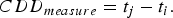 $$CDD_{measure} =t_j -t_i. $$
From the timeline, CDD measure is calculated as
 $$CDD_{measure} =e_1 +e_2 +CDD_{actual} +e_3 -e_4 -e_{5}. $$
Hence, the measurement error is
 $$e=e_{1} +e_{2} +e_{3} -e_{4} -e_{5} $$
Note that e 1, e 2, e 3, e 4, and e 5 are non-identical independent uniform random variables. The distribution of the sum of non-identical uniform random variables is given in [Reference Bradley and Gupta8].
For a random variable x which is the sum of n independent random variables, uniformly distributed in the intervals [c j − a j, c j + a j] for j = 1, 2,…, n, a j > 0, its probability density function is given by equation (14). In equation (14), the sum is over all 2n vectors of signs
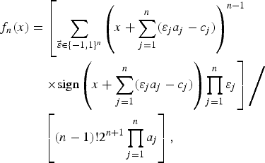 $$\eqalign{f_n \lpar x\rpar & = \left[\sum\limits_{\vec \varepsilon \in \lcub -1\comma 1\rcub^n} \left(x+\sum\limits_{j=1}^n \lpar \varepsilon_j a_j -c_j\rpar \right)^{n-1}\right. \cr & \left.\quad \times \hbox{sign} \left(x+\sum\limits_{j=1}^{n} \lpar \varepsilon_j a_j -c_j\rpar \right)\prod\limits_{j=1}^{n} \varepsilon_{j}\right]\left /\vphantom{\left(x+\sum\limits_{j=1}^{n} \lpar \varepsilon_j a_j -c_j\rpar \right)}\right. \cr & \quad \left[\lpar n-1\rpar !2^{n+1}\prod\limits_{j=1}^n {a_j} \right]\comma \; }$$
where
 $${\vec \varepsilon}=\lpar \varepsilon_1 \comma \; \varepsilon_2 \comma \; \ldots \comma \; \varepsilon_n \rpar \in {\lcub -1\comma \; 1 \rcub}^n \quad \hbox {i.e., each} \varepsilon_j = \pm 1, $$
and
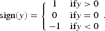 $$\hbox{sign}\lpar y\rpar = \left\{{\matrix{1 & {\hbox{if} y \gt 0} \cr 0 & {\hbox{if} y = 0} \cr -1 & {\hbox{if} y \lt 0} \cr } } \right. . $$
With equations (14)–(16), the distribution of measurement error in equation (13) can be expressed with n = 5,
 $$c =\left[\displaystyle{{T_{stamp}} \over {2}}\comma \; \displaystyle{{T_{pc\_screen}} \over {2}}\comma \; \displaystyle{{T_{c2\_screen}} \over {2}}\comma \; \displaystyle{{-T_{stamp}} \over {2}}\comma \; \displaystyle{{-T_{pc\_screen}} \over {2}}\right]\comma \; $$
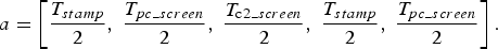 $$a = \left[\displaystyle{{T_{stamp}} \over {2}}\comma \; \displaystyle{{T_{pc\_screen}} \over {2}}\comma \; \displaystyle{{T_{{\rm c}2\_screen}} \over{2}}\comma \; \displaystyle{{T_{stamp}} \over {2}}\comma \; \displaystyle{{T_{pc\_screen}} \over {2}} \right].$$
The range of the measurement error is
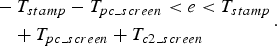 $$\eqalign{&-T_{stamp} -T_{pc\_screen} \lt e \lt T_{stamp} \cr & \quad + T_{pc\_screen} +T_{c2\_screen}}. $$
The expectation of the measurement error is
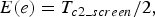 $$E\lpar e\rpar =T_{c2\_screen} / 2\comma \; $$
and the variance is the sum of five individual variance
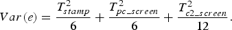 $$Var\lpar e\rpar = \displaystyle{{T_{stamp}^2} \over {6}} + \displaystyle{{T_{pc\_screen}^2} \over {6}} + \displaystyle{{T_{c2\_screen}^2} \over {12}}. $$
To verify this error distribution model, we simulate the sampling processes involved in Fig. 10 with the typical numbers in Table 2. We randomly set the sampling starting time of “timestamp generate”, “PC screen refresh”, “Cellphone1 capture”, “Cellphone2 display”, and “Webcam capture”. For each transmitted frame, we also randomly selected a network delay time associated with it. In one simulation the “Webcam” captures 100 times. Given starting time and delay time of this “transmission”, we can calculate the actual delay time for this 100 “capturing”. Also, knowing the time on two “captured frames”, the measured delay time can be calculated. With actual delay and measured delay of 100 capturing, 100 measurement errors can be obtained. We repeat the simulation 105 times with randomly selected starting time and delay time. The probability mass function of the total number of 107 errors is plotted in Fig. 11 with a time resolution of 1 ms. Note that the resolution is 1 ms, which makes the original continuous distribution to a discrete distribution, so a continuity correction (a 0.5 addition) [Reference Sheldon9] is applied. We also plot the density function derived by equation (14), with n = 5, c, and a in equations (17) and (18). From the figure, we can see the simulation results and the theoretical results match very well. The expectation of the measurement error is 8.5 ms, and the standard deviation is about 9.4 ms. These errors are usually acceptable in typical CDD measurement applications.
Fig. 11. Distribution of simulation results and the probability density function from equation (14).
From the above error analysis, our measurement is biased with T c2_screen/2. So we can subtract it from the final measurement. To reduce the variance, we can only reduce the timestamp interval, since T pc_screen and T c2_screen are intrinsic property of PC and Cellphone2. In Fig. 12, we show the measured error distribution with different T stamp.
Fig. 12. Distribution of errors with different T stamp. For shorter T stamp, the variance of errors is smaller.
Our error analysis models the capture and displaying processes as sampling processes. The lower bound and upper bound of the measurement error are [− T stamp − T pc_screen, T stamp + T pc_screen + T c2_screen]. After adjusting, the measurement is unbiased.
V. IMPLEMENTATION OF THE MEASUREMENT SYSTEM AND SIMULATION RESULTS
We have fully implemented the delay measurement system and successfully measured the CDD of many two-way visual communication applications over various networks.
A) Implementation details
Based on the error analysis discussed in the previous section, we select 10 ms as the T stamp in our experiments. Using 10 ms as the interval, we can omit the last (1 ms) digit of the timestamp, which can save space. Moreover, less number of digits can reduce the probability of recognition error. The associated measurement error is not significant for typical applications.
We use Bass Generator [10], a commercial QR-code generator Demo SDK, to encode the system time into a QR-code timestamp. With the space diversity and color diversity methods, although the multiple-overlapped-timestamp problem is solved, it could result in some faded QR-code patterns. In the QR-code recognition, CDD-R first carries out the binarization for every QR-code pattern. Our thresholding method used in the binarization is based on the Otsu algorithm [Reference Otsu11].
Due to non-uniform lighting, even within one timestamp pattern, the intensity may vary at different parts, as shown in Fig. 13(a). In this case, the top part is brighter than the bottom part. Using one global threshold may lose the information in the top part; a result is shown in Fig. 13(b). To overcome this problem, we split one QR-code into two half parts (top and bottom), and apply local thresholds derived by the Otsu algorithm. After performing the local binarization, we combine the two parts into one binary image, as shown in Fig. 13(c).
Fig. 13. (a) Intensity of pixels within one timestamp may vary due to the nonuniform lighting, (b) binarized image with one global threshold, and (c) binarized image with two local thresholds.
After binarization, the QR-code timestamp appearance is much enhanced. Experimental results show that the thresholding in the binarization contributes to improve the recognition accuracy significantly. The binary image is read using ZXing [12], an open source, multi-format one-dimensional/two-dimensional barcode reader. The reading accuracy of the QR-code shown on the LCD monitor reaches 99.7% and the one on the Cellphone2 screen is 95.0% in the experiments (see Section V). Given four columns of QR-codes, CDD-R recognizes all of them first. The columns without QR-code observed are removed. The timestamp with the latest time value is chosen as the time of the current video frame. When no recognition of the QR-code is successful, the system marks its time as “Invalid”.
A similar recognition process is run on the visual patterns combining two space and three color diversity. Three color components of the overlapped timestamps are extracted. Then the binarization is applied on each component. Combined with the space diversity of two, up to six possible timestamps can be recognized. Among these timestamps, the latest timestamp is selected as the time of the current frame.
B) Simulation results
The computer we used has a 3.1 GHz Intel Core i3-2100 CPU, 4 GB of RAM, and a NVIDIA GeForce 7600 GT graphics card. We use a Dell E2311H 23” widescreen monitor, with a refresh rate of 60 Hz. The machine runs the Windows 7 operating system. In our experiments, we pay special attention to the accuracy, precision, and the recognition time of different methods. There are roughly two steps of the timestamp recognition process: (1) read the pattern from the frame and (2) recognize the number of this pattern. Suppose there are M total received frames, among those M readable frames are read. Among these readable frames, timestamps on M correct frames are recognized correctly. Note that a readable timestamp cannot guarantee a correct timestamp because of possible recognition errors. The accuracy and precision are defined as follows:
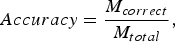 $$Accuracy = \displaystyle{{M_{correct}} \over {M_{total}}}\comma \; $$
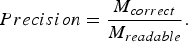 $$Precision = \displaystyle{{M_{correct}} \over {M_{readable}}}. $$
The Accuracy is the overall recognition accuracy and the Precision evaluates the effectiveness of the method of embedding time into a timestamp pattern (e.g. QR-code, human-readable digital numbers, and special rectangle visual patterns, as shown in the Section II). The processing time is the average processing time of all frames.
We tested the timestamps in digits without space diversity or color diversity as in Section IV. The accuracy and precision for the timestamps on the PC screen are 95.5 and 99.4%, respectively, which are good. However, the accuracy and precision for the timestamps on the Cellphone2 screen are only 17.2 and 46.9%, respectively. It means that among 25 frames, only about 12 frames are read successfully and only four frames are recognized correctly. The poor result is due to the multiple-overlapped-timestamp problem. We also investigated the recognition time. Without applying the proposed diversity scheme, it takes 30.7 ms/frame.
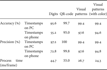
We then experiment the QR-code and the visual patterns we designed as shown in Fig. 3 with a space diversity of four. Table 3 shows the results. These results confirm the effectiveness of our proposed strategy. The precision of the QR-code reaches 100 and 99.8% for both the PC and Cellphone2 screens due to its checksum mechanism and error correction capability. The results using the visual patterns in Fig. 5 are also good.
Table 3. Accuracy, precision, and recognition time of timestamps recognition for one frame (resolution 720 × 1280).
We also test the visual patterns with space diversity of two + color diversity of three. The results are shown in the last column of Table 3. The accuracy and precision are similar to those using space diversity only. Note that the precision is slightly worse than w/o color diversity due to the error in color segmentation, but the main advantage of this method is that it takes less space and requires less time to recognize the timestamps.
Table 3 also shows the read time of a frame with a resolution  $720\times 1280$. The read time includes the recognition time and the selection time. The system needs to read two groups of timestamps (one on the PC screen and the other on the Cellphone2 screen) and select the latest time (among four columns due to the diversity of four) for each group separately. The system based on digits in Fig. 3(a) takes 44.7 ms/frame. The system based on the QR-code takes 55.0 ms to process a frame. The system based on the visual patterns in Fig. 5 without color diversity takes 26.7 ms/frame. The system based on the visual patterns in Fig. 9 with color diversity takes 24.3 ms/frame. It should be noted that we have not tried to optimize the speed of the code. With optimization, the speed should be able to be further improved. The QR-code takes more time due to its error correction function.
After recognizing the timestamps, we can perform error corrections. The timestamps can only go up. Also, for the timestamps marked “invalid”, they can be interpolated from the neighboring correctly recognized timestamps. Since it is difficult to simulate the network connection between two cellphones with a simulator, we test our measurement system over actual WiFi and 4 G networks. Figure 14 shows the final CDD of video chat sessions using FaceTime over the campus WiFi network and a 4 G network when the session is established through a stable wireless connection. To show the resultant figure clearly, we choose a typical video consisting of 500 frames to conduct the experiment. From the figure, we can clearly see that the delays of all frames in this example are relatively stable. Under WiFi network, the minimal delay is 160 ms, the maximal delay is 280 ms, the mean delay is 214 ms, and the standard deviation is about 21 ms. Under the 4 G network, the minimal delay is 200 ms, the maximal delay is 340 ms, the mean delay is 277 ms, and the standard deviation is about 27 ms.
Fig. 14. CDD of video chat sessions measured with the QR-code. (a) Facetime application over a WiFi network and (b) Facetime application over a 4| G network.
C) Discussion
The wireless network may not be very reliable, which may have long delay, narrow bandwidth, and packet loss. In this part, effects of these conditions are discussed as follows:
(1) Long delay
Our proposed model has no assumption that the delay should be short. In practice, to measure a long delay, a larger number of timestamps can be used which can represent a large time difference. In our real applications, considering the delay of our interest is always relatively short, we use a timestamp which can represent delay time up to 99.99 s and is long enough to measure the delay of most practical video chat applications.
(2) Narrow bandwidth and packet loss
Our proposed method does not assume that the receiver should receive all frames captured by the sender successfully. The encoder may discard some frames under a narrow bandwidth, or some frames may be lost due to the packet loss situations. However, as long as one frame is transmitted, received, and displayed on the receiver side, the delay associated with this frame can be measured.
VI. CONCLUSIONS
We developed an approach to measure the CDD of visual communication applications. The approach does not require modifications to any video application source code nor require access to the internal of the existing system. Also, it does not require the encoder and decoder clocks to be synchronized. The method is universal so that it can be used to measure the CDD of any visual communication applications. It has been successfully implemented in software. We investigated the multiple-overlapped-timestamp problem associated with the proposed approach and proposed a solution with space and color diversity. We analyze the distribution of the measurement error. Experimental results confirm the effectiveness of the proposed approach.
ACKNOWLEDGEMENTS
The authors would like to thank the support of Chao Wei and Mingli Song from the National High Technology Research and Development Program of China (863 Program) under grant No. 2013AA040601. The views presented are as individuals and do not necessarily reflect any position of T-Mobile USA.
Haoming Chen received the B.S. degree from Nanjing University, China in 2010 and the M.Phil. degree from Hong Kong University of Science and Technology in 2012, both in electrical engineering. He is currently pursuing the Ph.D. degree in the Electrical Engineering Department, University of Washington, Seattle, USA. He interned at Samsung Research America, Richardson, TX, USA and Apple, Cupertino, CA, USA, in the summer of 2013 and 2015, respectively. His research interests include video coding and processing, computer vision and multimedia communication. He is a recipient of the top 10% paper at IEEE ICIP 2014, and Student Best Paper Award Finalist at IEEE ISCAS 2012.
Chao Wei received the master's degree in computer science from Zhejiang University, Zhejiang, China, in 2014. His research interests include machine learning and computational advertising.
Mingli Song is currently a professor in Microsoft Visual Perception Laboratory and Zhejiang Provincial Key Lab of Service Robot, Zhejiang University. He received his Ph.D. degree in Computer Science and Technology from College of Computer Science, Zhejiang University, and B. Eng. Degree from Northwestern Polytechnical University. He was awarded Microsoft Research Fellowship in 2004. His research interests mainly include Computational Vision and Computer Graphics, and applications of Machine Learning in Vision and Graphics. He has authored and co-authored more than 90 scientific articles at top venues including IEEE T-PAMI, IEEE T-IP, T-MM, T-SMCB, Information Sciences, Pattern Recognition, CVPR, ECCV and ACM MM. He is an associate editor of Information Sciences, Neurocomputing and an editorial advisory board member of Recent Patent on Signal Processing. He has served with more than 10 major international conferences including ICDM, ACM Multimedia, ICIP, ICASSP, ICME, PCM, PSIVT and CAIP, and more than 10 prestigious international journals including T-IP, T-VCG, T-KDE, T-MM, T-CSVT, and TSMCB. He is a Senior Member of IEEE, and Professional Member of ACM.
Ming-Ting Sun received the B.S. degree in electrical engineering from National Taiwan University, Taipei, Taiwan, in 1976 and the Ph.D. degree in electrical engineering from University of California at Los Angeles, Los Angeles, CA, USA, in 1985. He joined University of Washington, Seattle, WA, USA, in 1996, where he is currently a Professor. He was the Director of the Video Signal Processing Research Group, Bellcore, Morristown, NJ, USA. He was a Chaired or Visiting Professor with Tsinghua University, Beijing, China; Tokyo University, Tokyo, Japan; National Taiwan University, National Cheng Kung University, Tainan, Taiwan; National Chung Cheng University, Chiayi, Taiwan; National Sun Yat-sen University, Kaohsiung, Taiwan; Hong Kong University of Science and Technology, Hong Kong; and National Tsing Hua University, Hsinchu, Taiwan. He has published over 200 technical papers, including 17 book chapters in video and multimedia technologies, and holds 13 patents. He is the co-editor of the book Compressed Video Over Networks. His research interests include video and multimedia signal processing, transport of video over networks, and very large-scale integration architecture and implementation.
Dr. Sun is currently the Editor-in-Chief of Journal of Visual Communications and Image Representation. He has been the Guest Editor of 11 special issues for various journals. He has given keynotes for several international conferences. He was a member of many prestigious award committees. He was a Technical Program Co-Chair of several conferences, including the 2010 International Conference on Multimedia and Expo. He was the Editor-in-Chief of IEEE TRANSACTIONS ON MULTIMEDIA and a Distinguished Lecturer of the Circuits and Systems Society from 2000 to 2001. He was the Editor-in-Chief of IEEE TRANSACTIONS ON CIRCUITS AND SYSTEMS FOR VIDEO TECHNOLOGY from 1995 to 1997. From 1988 to 1991 he was the Chairman of the IEEE CAS Standards Committee, and established the IEEE Inverse Discrete Cosine Transform Standard. He received the Award of Excellence from Bellcore for his work on the digital subscriber line in 1987, IEEE TRANSACTIONS ON CIRCUITS AND SYSTEMS FOR VIDEO TECHNOLOGY Best Paper Award in 1993, and the IEEE CASS Golden Jubilee Medal in 2000.
Kevin Lau is the Director of Device and Enabler Development at T-Mobile USA. He is passionate about building products and services that appeal to everyday mobile users. At T-Mobile, he is responsible for device and application development as well as system and architecture design. Prior to T-Mobile, Kevin worked at AT&T Wireless Services, Microsoft and Voicestream. He has a BSEE and MSEE degree from the University of Washington and has research interests in multimedia QoE over wireless networks. Kevin holds 7 patents on multimedia and wireless technologies.


 Open access